High-Dimensional Problems: p ≫ N
When there are many more features than observations, almost any flexible method can fit the training data perfectly, and the question becomes how to regularise. This chapter shows that heavy, simple regularisation wins: ridge with a large penalty, diagonal discriminant analysis with shrunken centroids, quadratic penalties computed in an \(N\)-dimensional space, the lasso and its relatives, kernels when only similarities are available, and supervised principal components for regression. It ends with the other side of high dimensions: assessing thousands of features at once, where the false discovery rate replaces the single p-value.
Ch. 1 Introduction Ch. 2 Supervised learning Ch. 3 Linear regression Ch. 4 Linear classification Ch. 5 Basis expansions Ch. 6 Kernel smoothing Ch. 7 Model assessment Ch. 8 Inference and averaging Ch. 9 Additive models and trees Ch. 10 Boosting Ch. 11 Neural networks Ch. 12 SVMs Ch. 13 Nearest neighbours Ch. 14 Unsupervised learning Ch. 15 Random forests Ch. 16 Ensembles Ch. 17 Graphical models Ch. 18 High-dimensional problems
How to read these notes
They follow the book. Sections carry the book's numbers (18.1, 18.2, ...) and every displayed equation that appears in the book carries the book's own equation number, e.g. \((18.15)\), so you can read these notes next to the book. Equations without a number are steps that the book skips.
Filling the gaps. Wherever the book says that something "can be shown", "is easy to check", leaves it to an exercise, or states a property without proof, an orange Filling the gap box or a proof gives the full argument. Proofs and derivations start hidden: open one with its bar, or use the button below.
Figures and demonstrations. Every figure of the chapter that is computed from data or a simulation is reproduced from scratch by the Python code, and Table 18.1 is recomputed. Several data sets used by the book are not on its website (the leukemia data with its test set, the protein mass spectra, the CGH profile, the protein sequences, the lymphoma survival data and the abstracts); where possible the figure is rebuilt on the closest available data or on a simulation that follows the book's description, and the caption says so. The ▶ Demo boxes open an interactive demonstration already set to the case being discussed.
Main reference
T. Hastie, R. Tibshirani and J. Friedman, The Elements of Statistical Learning: Data Mining, Inference, and Prediction, 2nd edition, Springer (2009), Chapter 18, pages 649–698 (book website, with the data sets: hastie.su.domains/ElemStatLearn). Section, equation, figure, table and exercise numbers below refer to this book. Further reading is listed in the references.
The explanations, derivations, figures and code are my own; equations are cited by their numbers in the book.
Companion courses
Parts of this chapter also appear in the companion courses on this site. The overlapping material is:
- Section 18.1 (ridge with \(p\) near or above \(N\), the minimum-norm interpolant and the error peak at \(p\approx N\)): Foundations of Deep Learning, Section 9.3.2, Filling the gap 9.7 and Result 9.8 (exact double descent); weight decay as ridge: Result 9.4.
- Section 18.3.5 (computing in the \(N\)-dimensional dual space) and Section 18.5.2 (kernel PCA): Bayesian and Probabilistic Machine Learning, Section 6.1 (dual representations), Section 12.1.4 (PCA for high-dimensional data) and Section 12.3 (kernel PCA).
- Section 18.6.1 (single-factor model and the principal component as its maximum-likelihood fit): Bayesian and Probabilistic Machine Learning, Section 12.2.1 (maximum-likelihood probabilistic PCA) and Section 12.2.4 (factor analysis).
- Section 18.7 (FWER, Bonferroni, the FDR, Benjamini–Hochberg, the two-groups model and the local fdr): Statistical Methods for Modern Biology, Section 6.8, Result 6.5 (Bonferroni), Result 6.6 (BH controls the FDR, with the full proof), Filling the gap 6.13 (BH as an estimated-FDR rule) and Result 6.7 (local and tail-area fdr); permutation tests: Result 6.4.
- Sections 18.2–18.4 in an applied setting (penalised classification of gene expression and microbiome data, soft thresholding, cross-validation): Statistical Methods for Modern Biology, Section 12.6.1, Result 12.16 and Filling the gap 12.4.
Within this course the chapter builds on Section 3.4.1 (ridge, its SVD form and degrees of freedom, Result 3.13), Section 3.4.2 and Result 3.16 (the lasso and its optimality conditions), Section 3.8.6 (coordinate descent), Section 3.5.2 (partial least squares), Section 4.3 and 4.3.1 (LDA and RDA), Section 4.4.4 (L1 logistic regression), Section 7.10.2 (cross-validation done right when features are screened) and Section 12.2 (the support vector classifier). New here: why ridge is the Bayes rule of Figure 18.1, the reduction theorem with its proof, the soft-thresholding property of the fused lasso, a short proof that BH controls the FDR, and notes on the book (Figure 18.1, positive dependence and the FWER, separability when p > N).
The chapter at a glance
- 18.1 With \(N=100\) and \(p=1000\), ridge needs a large penalty; in the simulation ridge with \(\lambda=\sigma^2\) is exactly the Bayes rule, and its risk bounds what any method can do (Result 18.1).
- 18.2 Diagonal LDA is nearest-centroid classification after scaling each gene (Result 18.2); soft-thresholding the standardised centroid contrasts selects genes, and is a lasso (Result 18.3).
- 18.3 Any linear model with a quadratic penalty can be fitted on the \(N\times N\) matrix \(\bR\) of \(\bX=\bR\bV^\T\) (Result 18.5); ridge reduces to (18.15) and tends to the minimum-norm interpolant (Result 18.6); multinomial ridge coefficients sum to zero (Result 18.4).
- 18.4 The lasso keeps at most \(N\) features (Result 18.7); the fused-lasso signal approximator is soft thresholding of a total-variation fit (Result 18.8).
- 18.5 Distances, centroids, medoids and principal components need only inner products, and squared distances become inner products by double centring (Result 18.9).
- 18.6 Supervised principal components: screen, then take a principal component, which is the maximum-likelihood estimate of the latent factor (Result 18.10).
- 18.7 Bonferroni bounds the FWER (Result 18.11); BH bounds the FDR by \(\alpha M_0/M\) (Result 18.12) and is the same rule as the permutation plug-in estimate (Result 18.13); the positive FDR is a posterior probability (Result 18.14).
Notation. Training data \((x_i,y_i)\) or \((x_i,g_i)\), \(i=1,\dots,N\), \(x_i\in\R^p\); \(\bX\) is the \(N\times p\) input matrix. \(\soft(z,\Delta)=\sgn(z)(|z|-\Delta)_+\) is soft thresholding. In Section 18.7 \(M\) is the number of features (hypotheses).
Prerequisites. Ridge and the lasso (Chapter 3), LDA and logistic regression (Chapter 4), the singular value decomposition, cross-validation (Chapter 7), and the support vector classifier (Chapter 12).
18.1 When \(p\) is Much Bigger than \(N\)
pp. 649–651 Gene-expression and proteomic studies measure thousands of features on tens or hundreds of samples. With \(p\gg N\) a linear model has more parameters than data, the training data can be fitted exactly, and the variance of any lightly regularised fit is enormous. The book's opening simulation makes the point with ridge regression. For each of \(N=100\) samples, \(p\) standard Gaussian features with pairwise correlation 0.2 are drawn, and
\[ Y=\sum_{j=1}^pX_j\beta_j+\sigma\varepsilon, \tag{18.1} \]with \(\varepsilon\sim N(0,1)\), the \(\beta_j\) drawn once per data set from \(N(0,1)\), and \(\sigma\) chosen so that \(\Var[\E(Y\given X)]/\sigma^2=2\). Ridge regression is fitted with \(\lambda=0.001\), \(100\) and \(1000\), for \(p=20\), \(100\) and \(1000\), and its test error is divided by the Bayes error \(\sigma^2\).
See also (companion course): Foundations of Deep Learning, Section 9.3.2, double descent, where the peak of the test error at \(p\approx N\) is derived exactly.
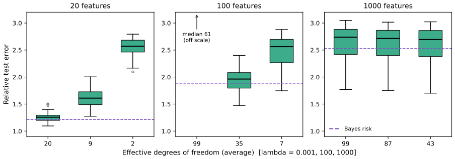
fig_18_1. Reproduces Hastie, Tibshirani and Friedman (2009), Figure 18.1. Download: PDF · SVGThe pattern is the book's: with \(p=20\) the lightest penalty wins (all 20 coefficients can be estimated), with \(p=100\) the middle one, and with \(p=1000\) the heaviest. The number of univariately "significant" coefficients (\(|\hb_j/\widehat{\mathrm{se}}_j|\ge2\) in a simple regression of \(y\) on \(x_j\)) averages 9.4, 36 and 300 in our runs (book: 9, 33 and 331): many coefficients are non-zero, but with \(N=100\) there is no hope of estimating 1000 of them, and the best one can do is shrink all of them hard. The degrees of freedom is the more interpretable index of the penalty: for fixed \(\lambda\) it depends on the inputs, so the figure shows its average.
Filling the gap 18.1: the effective degrees of freedom when \(p>N\), and why \(\lambda=0.001\) breaks down at \(p=100\) p. 650
Derivation
With an unpenalised intercept, ridge works on the centred inputs \(\bX_c=\bX-\bone\bar x^\T\), whose rank is at most \(\min(N-1,p)\). Write \(\bX_c=\bU\bD\bV^\T\) with \(d_1\ge\dots\ge d_r>0\), \(r=\rank\bX_c\). By Result 3.13 the fitted values are \(\bU\diag\{d_j^2/(d_j^2+\lambda)\}\bU^\T\by\) plus the mean, so
\[ \df(\lambda)=1+\sum_{j=1}^r\frac{d_j^2}{d_j^2+\lambda}, \]where the 1 counts the intercept; the book's (3.50) and Figure 18.1 count only the sum. As \(\lambda\to0\) the sum tends to \(r\): 20 for \(p=20\), and \(N-1=99\) for both \(p=100\) and \(p=1000\). So "99 df" means that the fit interpolates: the training residuals are zero.
The coefficient error is
\[ \hb-\bb=-\bV\diag\{\lambda/(d_j^2+\lambda)\}\bV^\T\bb+\bV\diag\{d_j/(d_j^2+\lambda)\}\bU^\T\boldsymbol\varepsilon\cdot\sigma \](plus the part of \(\bb\) outside the row space, which ridge cannot see when \(p>r\)). The noise part has covariance \(\sigma^2\bV\diag\{d_j^2/(d_j^2+\lambda)^2\}\bV^\T\), whose trace is
\[ \sigma^2\sum_jd_j^2/(d_j^2+\lambda)^2\approx\sigma^2\sum_j1/d_j^2 \]when \(\lambda\ll d_r^2\). For \(p=100\), \(N=100\) the centred design is \(100\times100\) of rank 99, an almost square Gaussian matrix, whose smallest singular values are close to zero (for a square Gaussian matrix the smallest singular value is of order \(1/\sqrt N\) times the typical one), so \(\sum1/d_j^2\) is huge and so is the test error. For \(p=20\) the smallest \(d_j^2\) is of order \(N(1-\sqrt{p/N})^2\), far from zero, and for \(p=1000\) it is of order \(p(1-\sqrt{N/p})^2\), also far from zero: only \(p\approx N\) is dangerous. This is the "double descent" peak of the companion course. ∎
Result 18.1 (ridge is the Bayes rule of the simulation, and the Bayes risk) Section 18.1
Suppose \(\bb\sim N(0,\bI_p)\) independently of the inputs, and \(\by\given\bX,\bb\sim N(\bX\bb,\sigma^2\bI)\) with \(\sigma^2\) known. Then the posterior mean of \(\bb\) is the ridge estimate without intercept at \(\lambda=\sigma^2\),
\[ \E(\bb\given\by,\bX)=(\bX^\T\bX+\sigma^2\bI)^{-1}\bX^\T\by,\qquad \Cov(\bb\given\by,\bX)=\sigma^2(\bX^\T\bX+\sigma^2\bI)^{-1}, \]and among all estimators \(\tilde\bb(\bX,\by)\) the one that minimises the average excess test error \(\E[(\tilde\bb-\bb)^\T\bSig(\tilde\bb-\bb)]\) is this posterior mean. Its relative test error, given the inputs, is
\[ \frac{\text{test error}}{\sigma^2}=1+\Tr\big[\bSig(\bX^\T\bX+\sigma^2\bI)^{-1}\big], \]with \(\bSig=0.8\bI+0.2\bone\bone^\T\) the covariance of a new input. Nothing can do better on average.
Proof
Posterior. The log posterior is \(-\|\by-\bX\bb\|^2/(2\sigma^2)-\|\bb\|^2/2\) plus a constant, a quadratic in \(\bb\) with Hessian \(-(\bX^\T\bX+\sigma^2\bI)/\sigma^2\) and maximiser \((\bX^\T\bX+\sigma^2\bI)^{-1}\bX^\T\by\). A Gaussian log density that is quadratic has its mean at the maximiser and covariance minus the inverse Hessian, which gives both formulas (Result 3.15).
Optimality. A new pair \((x_0,y_0)\) has \(y_0=x_0^\T\bb+\sigma\varepsilon_0\) with \(x_0\sim N(0,\bSig)\) independent of everything else, so for any \(\tilde\bb\) depending on the training data,
\[ \E[(y_0-x_0^\T\tilde\bb)^2\given\text{data},\bb]=\sigma^2+(\tilde\bb-\bb)^\T\bSig(\tilde\bb-\bb). \]Averaging over \(\bb\) given the data,
\[ \E[(\tilde\bb-\bb)^\T\bSig(\tilde\bb-\bb)\given\text{data}]=(\tilde\bb-m)^\T\bSig(\tilde\bb-m)+\Tr(\bSig C) \]with \(m\) and \(C\) the posterior mean and covariance, because the cross term has mean zero. The first term is non-negative and vanishes at \(\tilde\bb=m\). Dividing \(\sigma^2+\Tr(\bSig C)\) by \(\sigma^2\) gives the displayed risk. ∎
In the simulation \(\sigma^2=\bb^\T\bSig\bb/2\) depends on \(\bb\); its average is \(\Tr\bSig/2=p/2\) and its relative spread is small for large \(p\), so the code evaluates the bound at \(\sigma^2=p/2\) (bayes_rel_error, which computes the trace through \(N\times N\) matrices only). The bound explains the book's choice of penalties: the best \(\lambda\) is near \(\sigma^2\approx p/2\), that is 10, 50 and 500.
Note on the book: the error levels of Figure 18.1 for \(p=100\) and \(p=1000\)
In the book's figure the boxes for \(p=1000\) lie near 1.7–2.0 and the best box for \(p=100\) near 1.5. Under the model described in the text these values are below the Bayes risk of Result 18.1, which is 1.87 for \(p=100\) and 2.53 for \(p=1000\) (averaged over our designs; the spread across designs is tiny, minimum 2.52 for \(p=1000\)), so no method could reach them. Our reproduction gives medians 1.96 (\(p=100\), \(\lambda=100\)) and about 2.7 (\(p=1000\)), just above the bound, and the \(p=20\) panel agrees with the book's. The book's \(p=100\), \(\lambda=0.001\) box (about 2) is also hard to reconcile with an interpolating fit (Gap 18.1). Most likely the figure was produced with a different signal-to-noise ratio or error normalisation than the one stated; the qualitative conclusion (more shrinkage is better as \(p\) grows) is unaffected.
When \(p<N\), ridge with almost no penalty exploits the correlations between the features; when \(p\gg N\) there is not enough information to estimate a \(p\times p\) covariance matrix, and heavier regularisation predicts better. The rest of the chapter adapts \(N>p\) methods with heavy regularisation, or builds new ones, often using scientific context to choose the form of the regularisation.
18.2 Diagonal Linear Discriminant Analysis and Nearest Shrunken Centroids
pp. 651–654 The SRBCT data (Khan et al., 2001) are expression log-ratios of \(p=2308\) genes on 63 training samples of small round blue-cell tumours of four types, BL (8 samples), EWS (23), NB (12) and RMS (20), with 20 test samples. A full LDA needs the inverse of a \(2308\times2308\) within-class covariance of rank at most 59, so it is not defined. The simplest regularisation assumes that the features are independent within each class with a common variance per gene.
Definition 18.1 (diagonal LDA) p. 652, (18.2)–(18.3)
With class centroids \(\bar x_{kj}=\sum_{i\in C_k}x_{ij}/N_k\), the pooled within-class standard deviation \(s_j\) of gene \(j\) (divisor \(N-K\)) and priors \(\pi_k\), the diagonal LDA score of a test vector \(x^*\) for class \(k\) is
\[ \delta_k(x^*)=-\sum_{j=1}^p\frac{(x_j^*-\bar x_{kj})^2}{s_j^2}+2\log\pi_k, \tag{18.2} \]and the rule is
\[ C(x^*)=\ell\quad\text{if}\quad\delta_\ell(x^*)=\max_k\delta_k(x^*). \tag{18.3} \]The vector \(\tilde x_k=(\bar x_{k1},\dots,\bar x_{kp})^\T\) is the centroid of class \(k\).
Result 18.2 (diagonal LDA is Gaussian naive Bayes and a nearest-centroid rule) p. 652
(a) If within class \(k\) the features are independent \(N(\mu_{kj},\sigma_j^2)\), then \(2\log[\pi_kf_k(x)]=\delta_k(x)\) plus a term that does not depend on \(k\) when \(\mu_{kj},\sigma_j\) are replaced by \(\bar x_{kj},s_j\). Hence (18.3) is the plug-in Bayes rule, a special case of naive Bayes (Section 6.6.3), and LDA with the diagonal covariance \(\diag(s_1^2,\dots,s_p^2)\). (b) With equal priors, (18.3) assigns \(x^*\) to the nearest centroid in the metric that divides gene \(j\) by \(s_j\). (c) Under a common within-class variance \(\sigma^2\) for gene \(j\), \(\Var(\bar x_{kj}-\bar x_j)=m_k^2\sigma^2\) with \(m_k^2=1/N_k-1/N\), which is the scaling in (18.4).
Proof
(a)
\[ \log f_k(x)=-\sum_j(x_j-\mu_{kj})^2/(2\sigma_j^2)-\sum_j\log(\sqrt{2\pi}\sigma_j); \]the last sum does not depend on \(k\). Multiply by 2 and add \(2\log\pi_k\). (b) With equal priors, maximising \(\delta_k\) is minimising \(\sum_j(x_j^*-\bar x_{kj})^2/s_j^2\), a squared Euclidean distance after rescaling gene \(j\) by \(1/s_j\). (c) \(\bar x_j=\sum_\ell(N_\ell/N)\bar x_{\ell j}\), so
\[ \bar x_{kj}-\bar x_j=(1-N_k/N)\bar x_{kj}-\sum_{\ell\ne k}(N_\ell/N)\bar x_{\ell j}. \]The class means are independent with variances \(\sigma^2/N_\ell\), so the variance is
\[ (1-N_k/N)^2\sigma^2/N_k+\sum_{\ell\ne k}(N_\ell/N)^2\sigma^2/N_\ell=\sigma^2[(N-N_k)^2/(N^2N_k)+(N-N_k)/N^2]=\sigma^2(N-N_k)/(NN_k)=\sigma^2(1/N_k-1/N). \]∎
Bickel and Levina (2004) call this the independence rule and show that it can beat full LDA in high dimensions. On the SRBCT data it makes 5 errors on the 20 test samples, as in the book. It uses all 2308 genes, which is neither interpretable nor, as it turns out, optimal. Nearest shrunken centroids (NSC; Tibshirani et al., 2002) shrinks each class centroid towards the overall centroid, gene by gene. Let
\[ d_{kj}=\frac{\bar x_{kj}-\bar x_j}{m_k(s_j+s_0)}, \tag{18.4} \]where \(\bar x_j\) is the overall mean of gene \(j\), \(m_k^2=1/N_k-1/N\), and \(s_0\) is a small positive constant, usually the median of the \(s_j\), which stops genes with tiny variances from producing huge \(d_{kj}\). Each contrast is soft-thresholded,
\[ d'_{kj}=\sgn(d_{kj})(|d_{kj}|-\Delta)_+, \tag{18.5} \]or, alternatively, hard-thresholded,
\[ d'_{kj}=d_{kj}\cdot I(|d_{kj}|\ge\Delta), \tag{18.6} \]and the shrunken centroids are obtained by undoing (18.4),
\[ \bar x'_{kj}=\bar x_j+m_k(s_j+s_0)d'_{kj}. \tag{18.7} \]The shrunken centroids replace \(\bar x_{kj}\) in (18.2), with the scale \(s_j\) there replaced by \(s_j+s_0\) (this is what the shrunken-centroid classifier does, and it is what the code and demo use). Every \(d_{kj}\) moves towards zero by \(\Delta\) and becomes exactly zero once \(|d_{kj}|\le\Delta\); a gene whose four contrasts are all zero has \(\bar x'_{kj}=\bar x_j\) for every class and drops out of the comparison between classes.
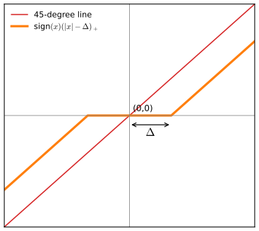
fig_18_2. Reproduces Hastie, Tibshirani and Friedman (2009), Figure 18.2. Download: PDF · SVGNote on the book: "less than zero" on p. 653
The sentence after (18.5) says that each \(d_{kj}\) "is set to zero if its absolute value is less than zero"; it should read "less than \(\Delta\)" (an absolute value is never negative).
Result 18.3 (soft thresholding of the centroids is a lasso) p. 653; Exercise 18.2
Fix gene \(j\), put \(\mu_j=\bar x_j\), and estimate the class effects \(\mu_{jk}\) by
\[ \min_{\mu_{j1},\dots,\mu_{jK}}\ \frac12\sum_{k=1}^K\sum_{i\in C_k}\frac{(x_{ij}-\bar x_j-\mu_{jk})^2}{s_j^2}+\lambda\sum_{k=1}^K\sqrt{N_k}\,\frac{|\mu_{jk}|}{s_j}. \]The solution is \(\hat\mu_{jk}=s_jm_k\,\soft(d_{kj},\lambda)\) with \(m_k=1/\sqrt{N_k}\) and \(d_{kj}=(\bar x_{kj}-\bar x_j)/(m_ks_j)\): exactly the shrunken contrast (18.5) and centroid (18.7) with \(\Delta=\lambda\), \(s_0=0\) and \(m_k^2=1/N_k\) in place of \(1/N_k-1/N\).
Proof
The problem separates over \(k\). For one class,
\[ \sum_{i\in C_k}(x_{ij}-c)^2=\sum_{i\in C_k}(x_{ij}-\bar x_{kj})^2+N_k(\bar x_{kj}-c)^2 \]for any constant \(c\), so up to a constant the class-\(k\) term is
\[ \tfrac12N_k(\bar x_{kj}-\bar x_j-\mu)^2/s_j^2+\lambda\sqrt{N_k}|\mu|/s_j. \]Substitute \(\mu=s_jm_k\delta\) with \(m_k=1/\sqrt{N_k}\): then
\[ N_k(\bar x_{kj}-\bar x_j-\mu)^2/s_j^2=N_km_k^2(d_{kj}-\delta)^2=(d_{kj}-\delta)^2 \]and \(\lambda\sqrt{N_k}|\mu|/s_j=\lambda|\delta|\). So \(\delta\) minimises \(\tfrac12(d_{kj}-\delta)^2+\lambda|\delta|\), whose solution is \(\soft(d_{kj},\lambda)\) (Result 5.15; the subgradient condition \(\delta-d_{kj}+\lambda\,\partial|\delta|\ni0\)). ∎
A caveat. If \(\mu_j\) is also minimised over, as in the book's (18.55), its stationarity condition is \(\mu_j=\bar x_j-\sum_k(N_k/N)\hat\mu_{jk}\), so \(\mu_j=\bar x_j\) only when \(\sum_kN_k\hat\mu_{jk}=0\). The joint minimiser is then a different lasso estimate: on the SRBCT data with \(\lambda=4\) (and \(s_0=0\)) both versions keep the same 345 genes and most centroids agree, but the joint fit moves a few shrunken centroids by up to 0.55 on the log-ratio scale. The exact equivalence holds with the overall mean held at \(\bar x_j\), which is how NSC is defined.
Figure 18.4 shows the effect of \(\Delta\). The threshold was chosen by 10-fold cross-validation; with \(\Delta=4.34\) only 43 genes survive (the book's number, reproduced exactly), and the classifier makes no training or test errors.
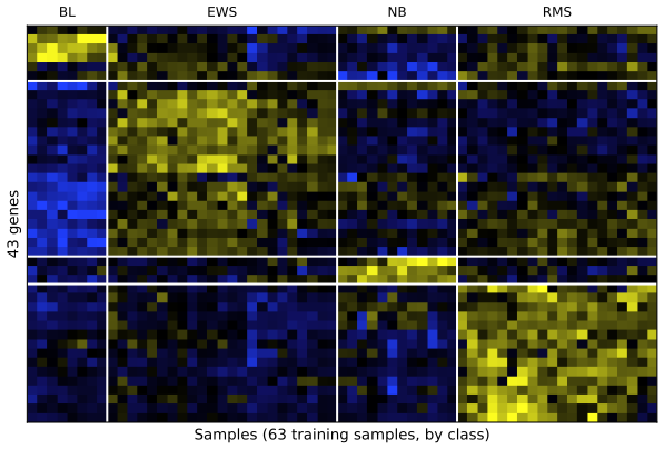
fig_18_3. Reproduces Hastie, Tibshirani and Friedman (2009), Figure 18.3. Download: PDF · SVG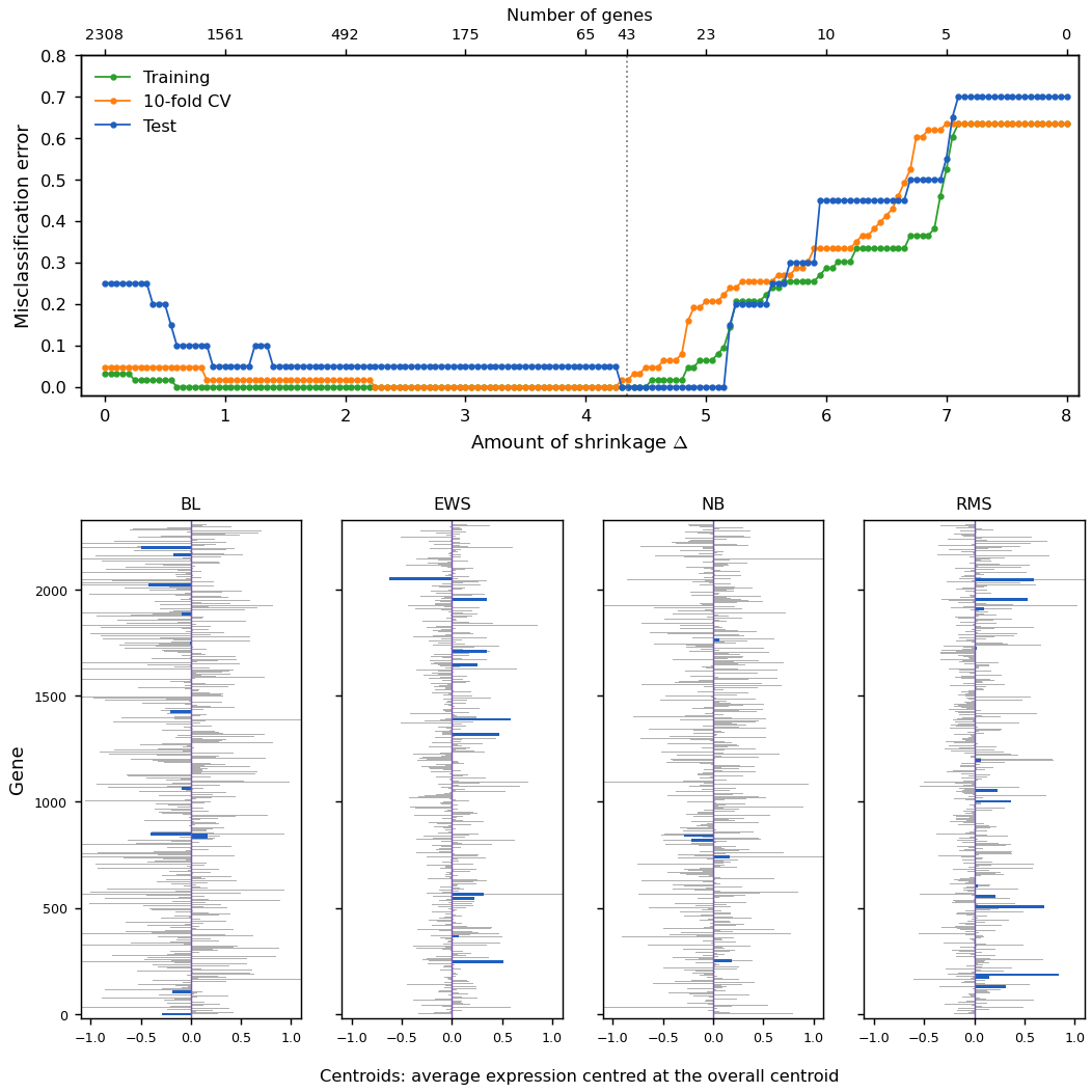
fig_18_4, NSC, nsc_cv. Reproduces Hastie, Tibshirani and Friedman (2009), Figure 18.4. Download: PDF · PNGThe discriminant scores also give class probabilities,
\[ \hat p_k(x^*)=\frac{e^{\frac12\delta_k(x^*)}}{\sum_{\ell=1}^Ke^{\frac12\delta_\ell(x^*)}}, \tag{18.8} \]which can rank the confidence of each call or flag a sample as unclassifiable.
Filling the gap 18.2: why (18.8) is the posterior probability p. 654
Derivation
By Result 18.2(a), under the independent-Gaussian model with the centroids and scales plugged in, \(\pi_kf_k(x)=c(x)\exp\{\tfrac12\delta_k(x)\}\) with \(c(x)\) the same for every class (it contains \(\prod_j(\sqrt{2\pi}s_j)^{-1}\)). Bayes' theorem gives \(\Pr(G=k\given x)=\pi_kf_k(x)/\sum_\ell\pi_\ell f_\ell(x)\), and \(c(x)\) cancels. The factor \(\tfrac12\) undoes the factor 2 in (18.2). With shrunken centroids the same formula is a plug-in posterior. ∎
Other forms of feature selection, such as hard thresholding, can be used; Fan and Fan (2008) show that some selection is essential for diagonal LDA in high dimensions, since accumulating noise over thousands of useless genes can make the independence rule no better than random guessing.
18.3 Linear Classifiers with Quadratic Regularization
pp. 654–656 The 14-cancer data of Ramaswamy et al. (2001) are harder: 144 training and 54 test patients, 14 cancer types, and \(p=16{,}063\) genes. Each patient's profile is first standardised to mean 0 and variance 1 across its genes (the shape of the profile matters more than its level). Table 18.1 compares eight classifiers; in each, the tuning parameter minimises the cross-validated error and, when several values tie, the test errors at the tied values are averaged.
Table 18.1 (recomputed): the 14-cancer data
| Method | CV errors (SE), out of 144 | Test errors, out of 54 | Genes used | Book: CV / test / genes |
|---|---|---|---|---|
| 1. Nearest shrunken centroids | 37 (4.5) | 17 | 4712 | 35 / 17 / 6520 |
| 2. L2-penalised discriminant analysis (18.9) | 25 (3.5) | 11.1 | 16,063 | 25 / 12 / 16,063 |
| 3. Support vector classifier (one versus all) | 25 (5.5) | 14 | 16,063 | 26 / 14 / 16,063 |
| 4. Lasso regression (one versus all) | 21 (6.0) | 14.2 | 1331 | 30.7 / 12.5 / 1429 |
| 5. \(k\)-nearest neighbours | 44 (5.5) | 24 | 16,063 | 41 / 26 / 16,063 |
| 6. L2-penalised multinomial (18.11) | 28 (5.0) | 11.5 | 16,063 | 26 / 15 / 16,063 |
| 7. L1-penalised multinomial (18.19) | 29 (4.8) | 17.5 | 180 | 17 / 13 / 269 |
| 8. Elastic-net penalised multinomial (18.21) | 20 (4.8) | 15.3 | 877 | 22 / 11.8 / 384 |
8-fold cross-validation with folds balanced by class (the same folds for every method); the standard error is that of the fold-average error, times 144. Methods 1, 2, 3, 5 and 6 are implemented in the course code, the last three through the \(144\times144\) reduction of Section 18.3.5 (the SVM through the inner products \(\bX\bX^\T\), method 6 on \(\bR=\bU\bD\), one reduction for all folds as in Exercise 18.12); methods 4, 7 and 8 use the R package glmnet. RDA: every \(\gamma\) from 0.02 to 0.99 gives the same cross-validated error (the book reports the same flatness over \(\gamma\in(0.002,0.55)\)); \(k\)-NN chooses \(k=3\); the SVM uses \(C=100\) (the errors do not depend on \(C\) once the training data are separated); the elastic net searches \(\alpha\in\{0.05,0.1,0.2,\dots,1\}\) and chooses \(\alpha\in[0.3,0.6]\). As the book stresses, each test error has a standard error of about 3, so most differences are within noise: seven of our eight cross-validated errors are within two standard errors of the book's. The exception is the L1-penalised multinomial (29 against 17, 2.5 standard errors), whose sparse solutions depend strongly on the folds and on where the path is cut; with our folds the elastic net (row 8) is the best method by cross-validation, as in the book. Code: table_18_1.
Regularised discriminant analysis, regularised multinomial logistic regression and the support vector machine try to use multivariate information; all three penalise the coefficients quadratically.
18.3.1 Regularized Discriminant Analysis
pp. 656–657 LDA needs the inverse of the \(p\times p\) within-class covariance \(\hat\bSig\), which has rank at most \(N-K\). RDA (Section 4.3.1) shrinks it towards its diagonal:
\[ \hat\bSig(\gamma)=\gamma\hat\bSig+(1-\gamma)\diag(\hat\bSig),\qquad\gamma\in[0,1]. \tag{18.9} \]\(\gamma=0\) is diagonal LDA, the unshrunken version of nearest shrunken centroids. The shrinkage resembles ridge regression, which shrinks the total covariance towards a multiple of the identity; through optimal scoring (LDA as a regression of scored class indicators, (12.58), Section 12.5) the analogy becomes exact. Guo et al. (2007) also shrink the centroids.
See also (this course): Section 4.3.1, regularized discriminant analysis and Filling the gap 4.5.
Filling the gap 18.3: computing RDA without a \(p\times p\) matrix p. 657; Exercise 18.6
Derivation
Let \(\bD=\diag(\hat\bSig)\) and rescale the inputs, \(\tilde x=\bD^{-1/2}x\). In these coordinates \(\tilde\bSig(\gamma)=\gamma\tilde\bSig+(1-\gamma)\bI\) with \(\tilde\bSig=\bW^\T\bW\), where the rows of \(\bW\) are the rescaled within-class residuals \((\tilde x_i-\tilde\mu_{g_i})^\T/\sqrt{N-K}\). Take the thin SVD \(\bW=\bU\bS\bV^\T\) (\(\bV\) is \(p\times r\), \(r\le N\)). Then
\[ \tilde\bSig(\gamma)=\bV\diag\{\gamma s_\ell^2+1-\gamma\}\bV^\T+(1-\gamma)(\bI-\bV\bV^\T), \]and for \(\gamma<1\) its inverse is
\[ \tilde\bSig(\gamma)^{-1}=\bV\diag\Big\{\frac{1}{\gamma s_\ell^2+1-\gamma}-\frac{1}{1-\gamma}\Big\}\bV^\T+\frac{1}{1-\gamma}\bI, \]as one checks by multiplying (the two pieces act on the orthogonal subspaces \(\span\bV\) and its complement). The LDA scores
\[ \tilde x^\T\tilde\bSig(\gamma)^{-1}\tilde\mu_k-\tfrac12\tilde\mu_k^\T\tilde\bSig(\gamma)^{-1}\tilde\mu_k+\log\pi_k \] therefore need only products with the \(p\times r\) matrix \(\bV\): the cost is that of one SVD of an \(N\times p\) matrix, \(O(pN^2)\), instead of \(O(p^3)\) (RDA in the code). Exercise 18.6 gives the same reduction through the theorem of Section 18.3.5. ∎
18.3.2 Logistic Regression with Quadratic Regularization
p. 657 With \(K\) classes the book uses the symmetric multinomial model
\[ \Pr(G=k\given X=x)=\frac{\exp(\beta_{k0}+x^\T\beta_k)}{\sum_{\ell=1}^K\exp(\beta_{\ell0}+x^\T\beta_\ell)}, \tag{18.10} \]with one coefficient vector per class, and maximises the penalised log-likelihood
\[ \max_{\{\beta_{0k},\beta_k\}_1^K}\Big[\sum_{i=1}^N\log\Pr(g_i\given x_i)-\frac\lambda2\sum_{k=1}^K\|\beta_k\|_2^2\Big]. \tag{18.11} \]The problem is concave in the coefficients (a sum of concave log-softmax terms and a concave penalty) and is solved by Newton's method or other smooth optimisers; Zhu and Hastie (2004) give details, and the code fits it by L-BFGS on the reduced inputs of Section 18.3.5 (multinomial_ridge).
Result 18.4 (the penalty resolves the redundancy) p. 657; Exercise 18.3
At the solution of (18.11), \(\sum_{k=1}^K\hat\beta_{kj}=0\) for every \(j=1,\dots,p\). The intercepts are not identified: adding the same constant to every \(\beta_{k0}\) leaves the likelihood unchanged, so one of them must be fixed (or their sum).
Proof
For any vector \(c\in\R^p\), replacing every \(\beta_k\) by \(\beta_k-c\) multiplies numerator and denominator of (18.10) by \(e^{-x^\T c}\), so the log-likelihood is unchanged. The penalty becomes \(\sum_k\|\beta_k-c\|^2\), which, as a function of \(c\), is a strictly convex quadratic minimised at \(c=\frac1K\sum_k\beta_k\). If the solution had \(\bar\beta=\frac1K\sum_k\hat\beta_k\ne0\), subtracting \(c=\bar\beta\) would keep the likelihood and strictly lower the penalty, contradicting optimality. Hence \(\bar\beta=0\). The intercepts are not penalised, so the same argument gives no condition on them; the likelihood is constant along \(\beta_{k0}\mapsto\beta_{k0}+c\) and the maximiser is a line, made unique by a convention such as \(\beta_{10}=0\) (used in the code) or \(\sum_k\beta_{k0}=0\). ∎
For separable two-class data, as \(\lambda\to0\) the coefficient vector of (18.11) diverges, but its direction converges to that of the maximal-margin separating hyperplane (Rosset, Zhu and Hastie, 2004), which makes penalised logistic regression an alternative to the SVM, especially with many classes.
Filling the gap 18.4: why the direction tends to the maximal margin p. 657
Derivation (sketch, no intercept)
Code \(y_i=\pm1\) and write the penalised loss as
\[ F_\lambda(\beta)=\sum_i\log(1+e^{-y_ix_i^\T\beta})+\tfrac\lambda2\|\beta\|^2. \]Let \(u^*\) be the unit vector maximising the minimum margin \(m(u)=\min_iy_ix_i^\T u\), with value \(m^*>0\) (separable data). Write \(\hat\beta_\lambda=t_\lambda u_\lambda\) with \(\|u_\lambda\|=1\). (i) \(t_\lambda\to\infty\): the loss part can be made as small as we like along \(tu^*\) while the penalty term \(\lambda t^2/2\) vanishes as \(\lambda\to0\), and for bounded \(t\) the loss is bounded away from zero. (ii) Using \(e^{-a}/2\le\log(1+e^{-a})\le e^{-a}\) for \(a\ge0\), the loss at \(tu\) is between \(\tfrac12e^{-tm(u)}\) and \(Ne^{-tm(u)}\) once every margin is positive. Compare \(\hat\beta_\lambda\) with \(t_\lambda u^*\), which has the same penalty: optimality gives \(\tfrac12e^{-t_\lambda m(u_\lambda)}\le Ne^{-t_\lambda m^*}\), i.e. \(m(u_\lambda)\ge m^*-\log(2N)/t_\lambda\). Since \(t_\lambda\to\infty\), \(m(u_\lambda)\to m^*\); the maximiser of the margin is unique (it is the solution of a strictly convex problem, Result 4.15) and \(m\) is continuous, so every limit point of \(u_\lambda\) is \(u^*\). With an unpenalised intercept the same argument works for the pair \((\beta_0,\beta)\) with the margin of Section 4.5.2. ∎
18.3.3 The Support Vector Classifier
pp. 657–658 The support vector classifier of Section 12.2 is attractive when \(p>N\) because the classes can then usually be separated by a hyperplane, and the unregularised (maximal-margin) classifier often does about as well as the best regularised one; the insensitivity of misclassification loss helps. For \(K>2\) classes, "one versus one" (ovo) fits all \(\binom K2\) pairwise classifiers and takes a vote; "one versus all" (ova) fits \(K\) classifiers of one class against the rest and picks the largest signed distance; Vapnik (1998) and Weston and Watkins (1999) propose genuinely multiclass criteria, and Tibshirani and Hastie (2007) arrange binary SVMs in a margin tree. Line 3 of Table 18.1 uses ova, which worked best here; its errors are insensitive to \(C\) above 0.001, and \(C=\infty\) separates the training data.
See also (companion course): Bayesian and Probabilistic Machine Learning, Section 7.1.3, multiclass SVMs.
Note on the book: when are the classes separable if \(p>N\)?
The book says the classes are perfectly separable "unless there are identical feature vectors in different classes". Distinct vectors are not enough. Three distinct points on a line in \(\R^p\) labelled \(+,-,+\) cannot be separated by any hyperplane, whatever \(p\) is: along the line a linear function is monotone. What is true is the following. If \(x_1,\dots,x_N\) are affinely independent (which needs \(p\ge N-1\), and holds with probability one for continuous data when \(p\ge N-1\)), every labelling is linearly separable. Proof: affine independence means the \(N\times(p+1)\) matrix with rows \((1,x_i^\T)\) has rank \(N\), so the linear system \(\beta_0+x_i^\T\beta=y_i\), \(i=1,\dots,N\), has a solution for any right-hand side, in particular \(y_i=\pm1\); the hyperplane \(\beta_0+x^\T\beta=0\) then separates the classes with every point at functional margin 1. ∎ With real data, near-collinearity can still make the margin tiny; this is the "data piling" of Exercise 18.8.
18.3.4 Feature Selection
pp. 658–659 None of the three quadratic methods selects features: every gene gets a non-zero weight. Ad hoc remedies remove the genes with the smallest weights and refit, backward stepwise (recursive feature elimination, Guyon et al., 2002); on these data it did not help, and the SVM's accuracy degrades as genes are removed from the full set of 16,063. The three methods can be made nonlinear with kernels, but with \(p\gg N\) the linear models are already complex enough; radial kernels sometimes help through robustness to outliers (far-apart points have damped inner products), but not on these data.
18.3.5 Computational Shortcuts When \(p\gg N\)
pp. 659–660 Every method in this section fits a linear model with a quadratic penalty, and for all of them the computation can be done in \(N\) dimensions instead of \(p\): \(N\) points in \(\R^p\) span a subspace of dimension at most \(N\). Let
\[ \bX=\bU\bD\bV^\T \tag{18.12} \] \[ \phantom{\bX}=\bR\bV^\T \tag{18.13} \]be the thin singular value decomposition: \(\bV\) is \(p\times N\) with orthonormal columns, \(\bU\) is \(N\times N\) orthogonal, \(\bD=\diag(d_1\ge d_2\ge\dots\ge d_N\ge0)\), and \(\bR=\bU\bD\) is \(N\times N\) with rows \(r_i^\T\). Ridge regression
\[ \hb=(\bX^\T\bX+\lambda\bI)^{-1}\bX^\T\by \tag{18.14} \]can be rewritten (Exercise 18.4, Result 18.6) as
\[ \hb=\bV(\bR^\T\bR+\lambda\bI)^{-1}\bR^\T\by. \tag{18.15} \]So \(\hb=\bV\hat\theta\), where \(\hat\theta\) is the ridge estimate on the \(N\) observations \((r_i,y_i)\): reduce \(\bX\) to \(\bR\) once and work with its rows. The cost falls from \(O(p^3)\) to \(O(pN^2)\).
Result 18.5 (the reduction theorem) p. 660, (18.16)–(18.17); Exercise 18.5
Let \(L(y,f)\) be any loss and \(f^*(r_i)=\theta_0+r_i^\T\theta\) with \(r_i\) from (18.13). Consider
\[ (\hat\beta_0,\hb)=\argmin_{\beta_0,\beta\in\R^p}\ \sum_{i=1}^NL(y_i,\beta_0+x_i^\T\beta)+\lambda\beta^\T\beta, \tag{18.16} \] \[ (\hat\theta_0,\hat\theta)=\argmin_{\theta_0,\theta\in\R^N}\ \sum_{i=1}^NL(y_i,\theta_0+r_i^\T\theta)+\lambda\theta^\T\theta. \tag{18.17} \]Then \(\hat\beta_0=\hat\theta_0\) and \(\hb=\bV\hat\theta\): the minimum values are equal, and the minimisers correspond one to one. (If the minimisers are not unique, the statement is that \((\theta_0,\theta)\mapsto(\theta_0,\bV\theta)\) maps the solution set of (18.17) onto that of (18.16).) The same holds for any number of coefficient vectors (multinomial models, neural networks with weight decay on the first layer) and for a positive semidefinite penalty \(\lambda\beta^\T\bP\beta\) whose matrix commutes with the projection \(\bV\bV^\T\) (then (18.17) uses \(\lambda\theta^\T\bV^\T\bP\bV\theta\)).
Proof
Since \(\bX=\bR\bV^\T\), row \(i\) of \(\bX\) is \(x_i=\bV r_i\), so \(x_i^\T\beta=r_i^\T\bV^\T\beta\). Decompose any \(\beta\in\R^p\) as \(\beta=\bV\theta+\beta_\perp\) with \(\theta=\bV^\T\beta\) and \(\bV^\T\beta_\perp=0\) (the projection onto the column space of \(\bV\) and its orthogonal complement). Then
\[ x_i^\T\beta=r_i^\T\bV^\T\bV\theta+r_i^\T\bV^\T\beta_\perp=r_i^\T\theta,\qquad \beta^\T\beta=\theta^\T\bV^\T\bV\theta+\|\beta_\perp\|^2=\theta^\T\theta+\|\beta_\perp\|^2. \]So the objective of (18.16) at \((\beta_0,\beta)\) equals the objective of (18.17) at \((\beta_0,\theta)\) plus \(\lambda\|\beta_\perp\|^2\). For fixed \((\beta_0,\theta)\) this is minimised, uniquely when \(\lambda>0\), by \(\beta_\perp=0\). Hence \(\min(18.16)=\min(18.17)\), and \((\beta_0,\beta)\) solves (18.16) if and only if \(\beta_\perp=0\) and \((\beta_0,\bV^\T\beta)\) solves (18.17), i.e. \(\beta=\bV\theta\) with \((\beta_0,\theta)\) a solution of (18.17). Nothing about \(L\) was used except that it depends on \(\beta\) only through the fitted values. ∎
Geometrically, rotate the feature space so that all but the first \(N\) coordinates of every observation are zero: the quadratic penalty is invariant under rotations and a linear model is equivariant, so the extra coordinates only add penalty and are set to zero. The argument fails for the lasso: \(\|\beta\|_1\) is not rotation invariant, and \(\|\bV\theta+\beta_\perp\|_1\) does not split.
Typically \(\lambda\) is chosen by cross-validation. By Exercise 18.12, \(\bR\) needs to be computed only once, on all the data: the rows of \(\bX\) in any fold still lie in the column space of \(\bV\), and the proof above only used that. The kernel trick of Section 12.3.7 is the same reduction: \(\bK=\bX\bX^\T=\bU\bD^2\bU^\T\) carries the same information as \(\bR\), and Exercise 18.13 fits ridged logistic regression from \(\bK\) alone.
See also (companion course): Bayesian and Probabilistic Machine Learning, Section 6.1, dual representations.
Result 18.6 (ridge in \(N\) dimensions, and its limit) (18.14)–(18.15), (18.56); Exercises 18.4 and 18.7
For \(\lambda>0\),
\[ \hb_\lambda=(\bX^\T\bX+\lambda\bI)^{-1}\bX^\T\by=\bX^\T(\bX\bX^\T+\lambda\bI)^{-1}\by=\bV(\bR^\T\bR+\lambda\bI)^{-1}\bR^\T\by. \]If \(\rank\bX=N<p\), then as \(\lambda\downarrow0\), \(\hb_\lambda\to\hb_0=\bV\bD^{-1}\bU^\T\by=\bX^+\by\), the solution of \(\bX\beta=\by\) with the smallest Euclidean norm.
Proof
First identity. \((\bX^\T\bX+\lambda\bI)\bX^\T=\bX^\T(\bX\bX^\T+\lambda\bI)\); multiply on the left by \((\bX^\T\bX+\lambda\bI)^{-1}\) and on the right by \((\bX\bX^\T+\lambda\bI)^{-1}\) (both positive definite). This also shows \(\hb_\lambda=\bX^\T s\) with \(s=(\bX\bX^\T+\lambda\bI)^{-1}\by\in\R^N\), the book's hint. Second. Substitute \(\bX=\bR\bV^\T\): \(\bX\bX^\T=\bR\bR^\T\) and \(\bX^\T=\bV\bR^\T\), so
\[ \hb_\lambda=\bV\bR^\T(\bR\bR^\T+\lambda\bI)^{-1}\by=\bV(\bR^\T\bR+\lambda\bI)^{-1}\bR^\T\by \]by the first identity applied to \(\bR\). Limit. With \(\bR=\bU\bD\),
\[ (\bR^\T\bR+\lambda\bI)^{-1}\bR^\T=\diag\{d_j/(d_j^2+\lambda)\}\bU^\T\to\bD^{-1}\bU^\T \]since all \(d_j>0\). The limit solves \(\bX\beta=\bU\bD\bV^\T\bV\bD^{-1}\bU^\T\by=\by\). Every solution of \(\bX\beta=\by\) is \(\hb_0+n\) with \(\bX n=0\), i.e. \(\bV^\T n=0\); since \(\hb_0\) lies in the column space of \(\bV\), \(\|\hb_0+n\|^2=\|\hb_0\|^2+\|n\|^2\), so \(\hb_0\) has the smallest norm, uniquely. ∎
18.4 Linear Classifiers with L1 Regularization
pp. 661–664 The quadratic methods keep every feature. An L1 penalty selects. The lasso of Section 3.4.2 in Lagrange form (3.52) is
\[ \min_\beta\ \frac12\sum_{i=1}^N\Big(y_i-\beta_0-\sum_{j=1}^px_{ij}\beta_j\Big)^2+\lambda\sum_{j=1}^p|\beta_j|. \tag{18.18} \]LARS (Section 3.8.1) computes the whole path. When \(p>N\) the lasso fits the training data exactly as \(\lambda\to0\), and it never needs more than \(N\) non-zero coefficients.
See also (this course): Result 3.16, the optimality conditions of the lasso, and Result 3.19, LAR computes the lasso path.
Result 18.7 (at most \(N\) non-zero coefficients) p. 661
For every \(\lambda>0\), (18.18) has a solution with at most \(\min(N,p)\) non-zero coefficients (at most \(N-1\) with the intercept, since the centred inputs have rank at most \(N-1\)). If the columns of \(\bX\) are in general position (a condition made precise by Tibshirani (2013), which holds with probability one when the inputs have a continuous distribution), the solution is unique and therefore has at most \(N\) non-zero entries.
Proof of the first statement
Work with the centred \(\bX\) and \(\by\) (the intercept is then \(\bar y-\bar x^\T\hb\)). All solutions have the same fitted vector \(\hat\mu=\bX\hb\) (the loss is strictly convex in \(\bX\beta\) and the penalty is convex, so two solutions with different fits would have a strictly better midpoint). Take a solution \(\hb\) with support \(A\) and suppose the columns \(\{x_j:j\in A\}\) are linearly dependent, \(\bX_A c=0\) with \(c\ne0\). The KKT conditions (Result 3.16) give \(x_j^\T(\by-\hat\mu)=\lambda\,\sgn(\hb_j)\) on \(A\); as \(\hat\mu\) is common to all solutions, so are these signs. Since \(\bX_Ac=0\) we get \(\sum_{j\in A}c_j\sgn(\hb_j)\lambda=(\by-\hat\mu)^\T\bX_Ac=0\). Now move along \(\hb+tc\) (on \(A\)): the fit does not change, and as long as no coordinate changes sign the penalty is \(\lambda\sum_{j\in A}\sgn(\hb_j)(\hb_j+tc_j)\), whose derivative in \(t\) is zero. So every such point is a solution. Increase \(|t|\) until the first coordinate reaches zero: we get a solution with smaller support. Repeat until the columns of the support are independent; then the support size is at most \(\rank\bX\le\min(N,p)\). ∎ Uniqueness under general position is proved by Tibshirani (2013).
Lasso regression can classify two classes by coding \(\pm1\) and thresholding at zero; for more classes, ova or ovo. Line 4 of Table 18.1 uses ova. A more natural approach penalises the multinomial likelihood (Friedman, Hastie and Tibshirani, 2010):
\[ \max_{\{\beta_{0k},\beta_k\in\R^p\}_1^K}\Big[\sum_{i=1}^N\log\Pr(g_i\given x_i)-\lambda\sum_{k=1}^K\sum_{j=1}^p|\beta_{kj}|\Big], \tag{18.19} \]solved by cyclical coordinate descent (Section 3.8.6) at a decreasing sequence of \(\lambda\), with warm starts and the sparsity of the solutions when \(p\gg N\). Line 7 of Table 18.1 uses it. Genes in a pathway are strongly correlated; the lasso is indifferent among a group of strong correlated features (Exercise 3.28), ridge shrinks their coefficients towards each other (Exercise 3.29), and the elastic net (Zou and Hastie, 2005) compromises:
\[ \sum_{j=1}^p\big(\alpha|\beta_j|+(1-\alpha)\beta_j^2\big). \tag{18.20} \]With this penalty the multinomial problem is
\[ \max_{\{\beta_{0k},\beta_k\in\R^p\}_1^K}\Big[\sum_{i=1}^N\log\Pr(g_i\given x_i)-\lambda\sum_{k=1}^K\sum_{j=1}^p\big(\alpha|\beta_{kj}|+(1-\alpha)\beta_{kj}^2\big)\Big], \tag{18.21} \]which can select more than \(N\) features. (The software, and our code, write the quadratic part as \((1-\alpha)\beta^2/2\); this only rescales \(\alpha\).)
Filling the gap 18.5: why the elastic net averages correlated features p. 662
Derivation
Take the regression form
\[ \tfrac12\|\by-\bX\beta\|^2+\lambda[\alpha\|\beta\|_1+\tfrac{1-\alpha}2\|\beta\|^2] \]with standardised columns and \(\alpha<1\), so the objective is strictly convex and the solution unique. (i) Identical features. If \(x_j=x_k\) and \((\hb_j,\hb_k)\) were different, swapping them leaves the loss and the L1 term unchanged, so swapping gives another solution; uniqueness forces \(\hb_j=\hb_k\). The lasso (\(\alpha=1\)) has a whole segment of solutions instead and the algorithm picks one end. (ii) Correlated features (Zou and Hastie, 2005). If \(\hb_j\hb_k>0\), subtracting the stationarity conditions
\[ x_j^\T(\by-\bX\hb)=\lambda\alpha\,\sgn\hb_j+\lambda(1-\alpha)\hb_j \]for \(j\) and \(k\) gives \(\lambda(1-\alpha)(\hb_j-\hb_k)=(x_j-x_k)^\T(\by-\bX\hb)\), so
\[ |\hb_j-\hb_k|\le\frac{\|x_j-x_k\|\,\|\by-\bX\hb\|}{\lambda(1-\alpha)}\le\frac{\sqrt{2(1-\rho_{jk})}\,\|\by\|}{\lambda(1-\alpha)}, \]using \(\|\by-\bX\hb\|\le\|\by\|\) (the objective at \(\hb\) is at most its value at 0) and \(\|x_j-x_k\|^2=2(1-\rho_{jk})\) for unit-norm columns with correlation \(\rho_{jk}\). Highly correlated features get nearly equal coefficients. ∎
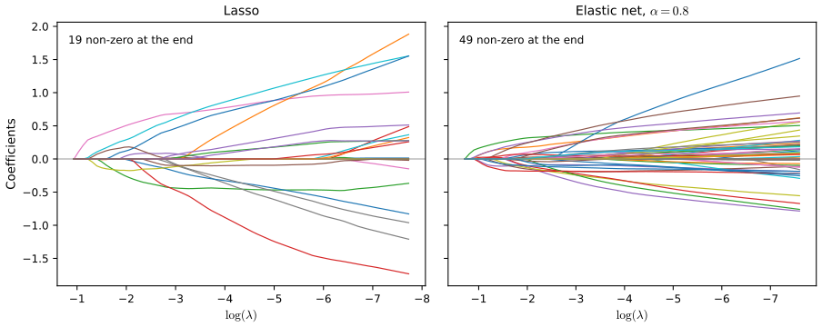
logistic_enet_path), which agrees with glmnet. Code: fig_18_5. Reproduces Hastie, Tibshirani and Friedman (2009), Figure 18.5. Download: PDF · SVG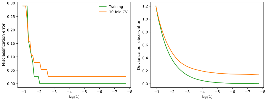
fig_18_6, leukemia_paths. Reproduces Hastie, Tibshirani and Friedman (2009), Figure 18.6. Download: PDF · SVGFor \(p\gg N\) the coefficients of every penalised logistic model diverge as \(\lambda\to0\) (Exercise 18.11), so software stops at some positive \(\lambda\). The renormalised coefficients converge: for \(\alpha=0\) to the SVM direction (Gap 18.4), for \(\alpha=1\) to an L1-margin separating hyperplane with at most \(N\) genes (Rosset et al., 2004), and in between to hyperplanes with more genes as \(\alpha\) decreases.
See also (this course): Result 4.11, the L1 logistic problem, and Filling the gap 4.11, separable data.
18.4.1 Application of Lasso to Protein Mass Spectroscopy
pp. 664–666 Mass spectrometry measures, for each blood-serum sample, the intensity at many time-of-flight values, which correspond to mass over charge (m/z) of the proteins; peaks indicate proteins. The prostate-cancer data of Adam et al. (2002; cited as 2003 in the book) have 16,898 m/z sites between 2000 and 40,000, 157 healthy and 167 cancer patients (Figure 18.7 shows the average spectra). These data are not on the book's website, so Figure 18.7 and Table 18.2 are not reproduced. The book's findings: on 108 test spectra, nearest shrunken centroids makes 34 errors with 459 sites, the lasso 22 errors with 113 sites, and the lasso on 728 common peaks (found by hierarchical clustering of the peak positions on the log m/z scale, cut at log(0.005), i.e. peaks less than 0.5% apart are merged) 28 errors with 35 peaks. Fitting harder wins on error, but the peak-based model is more useful scientifically, because the lasso on raw sites does not respect peaks, and the same protein appears at slightly shifted m/z in different spectra.
18.4.2 The Fused Lasso for Functional Data
pp. 666–668 When the features have a natural order (m/z, genome position, time), one can expand the coefficient function in a basis (Section 5.3) or penalise its roughness (Section 12.6). Those methods smooth uniformly. The fused lasso (Tibshirani et al., 2005) adapts to jumps:
\[ \min_{\beta\in\R^p}\Big\{\sum_{i=1}^N\Big(y_i-\beta_0-\sum_{j=1}^px_{ij}\beta_j\Big)^2+\lambda_1\sum_{j=1}^p|\beta_j|+\lambda_2\sum_{j=1}^{p-1}|\beta_{j+1}-\beta_j|\Big\}. \tag{18.22} \]The first penalty makes the solution sparse, the second makes it piecewise constant in \(j\). (The book calls the criterion strictly convex; it is strictly convex in \(\beta\) only when \(\bX\) has full column rank, which fails when \(p>N\). It is always convex, so its minimum value and fitted values are unique, and for the signal approximator below, where \(\bX=\bI\), the solution is unique.) For unequally spaced \(t_j\) use divided differences:
\[ \lambda_2\sum_{j=1}^{p-1}\frac{|\beta_{j+1}-\beta_j|}{|t_{j+1}-t_j|}. \tag{18.23} \]With \(\bX=\bI_N\) one gets the fused lasso signal approximator for a sequence \(y_1,\dots,y_N\):
\[ \min_{\beta\in\R^N}\Big\{\sum_{i=1}^N(y_i-\beta_0-\beta_i)^2+\lambda_1\sum_{i=1}^N|\beta_i|+\lambda_2\sum_{i=1}^{N-1}|\beta_{i+1}-\beta_i|\Big\}. \tag{18.24} \](With \(\lambda_1=0\) the intercept \(\beta_0\) is not identifiable, since only \(\beta_0+\beta_i\) appears; it is usually dropped, as we do.)
Result 18.8 (the signal approximator is soft-thresholded total variation) p. 667; Friedman et al. (2007)
Let \(\hat b\) solve \(\min_b\tfrac12\|y-b\|^2+\lambda_2\sum_i|b_{i+1}-b_i|\) (total-variation denoising, \(\lambda_1=0\)). Then for every \(\lambda_1\ge0\) the solution of
\[ \min_b\tfrac12\|y-b\|^2+\lambda_1\sum_i|b_i|+\lambda_2\sum_i|b_{i+1}-b_i| \]is \(\soft(\hat b,\lambda_1)\), applied coordinate by coordinate. ((18.24) without \(\beta_0\) is this problem with \(\lambda_1,\lambda_2\) halved.)
Proof
Write \(D\) for the \((N-1)\times N\) first-difference matrix. The optimality condition of the total-variation problem is \(y-\hat b=D^\T\hat u\) with
\[ \hat u_i\in\lambda_2\,\partial|\cdot|(\hat b_{i+1}-\hat b_i), \]i.e. \(|\hat u_i|\le\lambda_2\) and \(\hat u_i=\lambda_2\sgn(\hat b_{i+1}-\hat b_i)\) when the difference is non-zero. Put \(b^*=\soft(\hat b,\lambda_1)\). We must find \(u,v\) with \(y-b^*=D^\T u+v\), \(u_i\in\lambda_2\partial|\cdot|(b^*_{i+1}-b^*_i)\) and \(v_i\in\lambda_1\partial|\cdot|(b^*_i)\). Take \(u=\hat u\) and \(v=\hat b-b^*\). Then \(D^\T u+v=y-\hat b+\hat b-b^*=y-b^*\). (1) \(v_i=\hat b_i-\soft(\hat b_i,\lambda_1)\) equals \(\lambda_1\sgn(\hat b_i)=\lambda_1\sgn(b^*_i)\) when \(|\hat b_i|>\lambda_1\) and equals \(\hat b_i\in[-\lambda_1,\lambda_1]\) when \(b^*_i=0\): a valid subgradient. (2) Soft thresholding is non-decreasing, so \(b^*_{i+1}-b^*_i\) has the same sign as \(\hat b_{i+1}-\hat b_i\) or is zero. If it is non-zero, the sign is that of \(\hat b_{i+1}-\hat b_i\), and \(\hat u_i=\lambda_2\) times that sign; if it is zero, any \(|\hat u_i|\le\lambda_2\) is valid. So \(\hat u\) is a valid subgradient at \(b^*\). The problem is strictly convex, so \(b^*\) is its unique solution. ∎
The total-variation part is solved through its dual, a box-constrained quadratic programme in \(N-1\) variables, by L-BFGS-B followed by an exact active-set step (tv_denoise); the solution agrees with a direct solve of the full problem to about \(10^{-7}\).
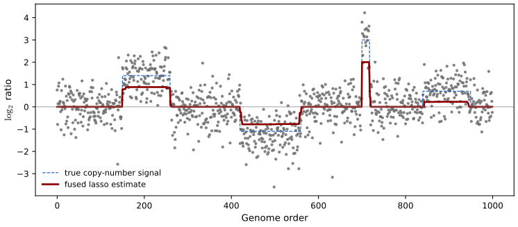
fig_18_8, flsa. Reproduces Hastie, Tibshirani and Friedman (2009), Figure 18.8. Download: PDF · SVGA two-dimensional version penalises differences with the four neighbours of each pixel, for denoising or classifying images; Friedman et al. (2007) give coordinate-descent algorithms for both.
18.5 Classification When Features are Unavailable
p. 668 Sometimes the objects (protein structures, documents) have no natural feature vector, or a huge one. As long as an \(N\times N\) matrix of similarities can be filled in and read as inner products, many classifiers still apply. Pairwise distances serve as well, because they can be turned into centred inner products (Result 18.9). Proximity matrices are treated in Chapter 14.
18.5.1 Example: String Kernels and Protein Classification
pp. 668–670 Proteins are strings over the 20 amino acids, of varying lengths. Leslie et al. (2004) compare two strings through the substrings of length \(m\) they share. With \(\mathcal A_m\) the set of the \(20^m\) strings of length \(m\) and \(\phi_a(x)\) the number of times \(a\) occurs in \(x\), the feature map and kernel are
\[ \Phi_m(x)=\{\phi_a(x)\}_{a\in\mathcal A_m}, \tag{18.25} \] \[ K_m(x_1,x_2)=\langle\Phi_m(x_1),\Phi_m(x_2)\rangle. \tag{18.26} \]For \(m=4\) the feature space has \(160{,}000\) dimensions, but a string of length \(L\) has at most \(L-m+1\) non-zero features, so the kernel matrix can be computed without forming the vectors: with tries or suffix trees (Leslie et al.), or, as in our code, as a sparse matrix of counts whose product with its transpose is \(\bK\). The kernel is positive semidefinite by construction, being a Gram matrix.
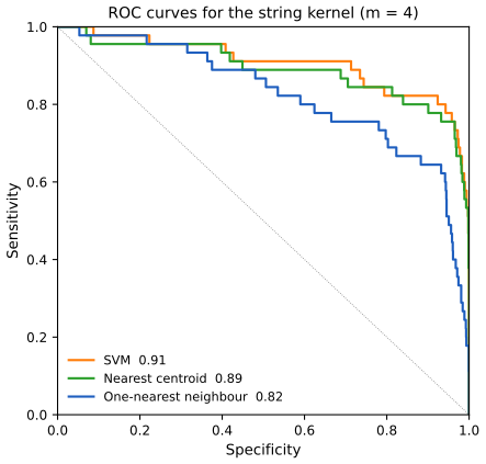
fig_18_9, protein_sim, string_kernel. Reproduces Hastie, Tibshirani and Friedman (2009), Figure 18.9. Download: PDF · SVG18.5.2 Classification and Other Models Using Inner-Product Kernels and Pairwise Distances
pp. 670–672 Any method that touches the data only through inner products can be "kernelised". Nearest neighbours need distances, which inner products give:
\[ \|x_i-x_{i'}\|^2=\langle x_i,x_i\rangle+\langle x_{i'},x_{i'}\rangle-2\langle x_i,x_{i'}\rangle. \tag{18.27} \]A distance-weighted 1-NN rule gives a continuous score for the ROC curve (Exercise 18.14). Nearest centroids follow as well: for training pairs \((x_i,g_i)\), a test point \(x_0\) and class centroids \(\bar x_k\),
\[ \|x_0-\bar x_k\|^2=\langle x_0,x_0\rangle-\frac2{N_k}\sum_{g_i=k}\langle x_0,x_i\rangle+\frac1{N_k^2}\sum_{g_i=k}\sum_{g_{i'}=k}\langle x_i,x_{i'}\rangle, \tag{18.28} \](expand \(\|x_0-\frac1{N_k}\sum_{g_i=k}x_i\|^2\); the book's display drops the \(1/N_k\) in front of the middle sum's index set only typographically), and so do \(K\)-means clustering, quadratically penalised logistic regression (Exercise 18.13) and LDA (Exercise 12.10). Principal components need only \(\bK\): if \(\bX\) is centred with SVD \(\bU\bD\bV^\T\), the component scores are \(\bZ=\bU\bD\), and \(\bK=\bX\bX^\T=\bU\bD^2\bU^\T\); an uncentred \(\bX\) is centred by \(\tilde\bX=(\bI-\bM)\bX\), \(\bM=\bone\bone^\T/N\), so one takes the eigenvectors of \((\bI-\bM)\bK(\bI-\bM)\) (Exercise 18.15; kernel PCA, Section 14.5.4). If only squared distances
\[ \Delta_{ii'}^2=\|x_i-x_{i'}\|^2 \tag{18.29} \]are available, write
\[ \Delta_{ii'}^2=\|x_i-\bar x\|^2+\|x_{i'}-\bar x\|^2-2\langle x_i-\bar x,x_{i'}-\bar x\rangle, \tag{18.30} \]set \(\bB=\{-\Delta^2_{ii'}/2\}\) and double centre:
\[ \tilde\bK=(\bI-\bM)\bB(\bI-\bM). \tag{18.31} \]See also (companion course): Bayesian and Probabilistic Machine Learning, Section 12.3, kernel PCA; and the multidimensional scaling demo of Statistical Methods for Modern Biology, which uses (18.31).
Result 18.9 (double centring recovers the centred inner products) p. 671, (18.30)–(18.31)
\(\tilde K_{ii'}=\langle x_i-\bar x,x_{i'}-\bar x\rangle\) for all \(i,i'\), where \(\bar x=\frac1N\sum_ix_i\). In particular \(\tilde\bK\) is positive semidefinite, and its eigenvectors give the principal-component scores.
Proof
Put \(z_i=x_i-\bar x\), so \(\sum_iz_i=0\), and \(a_i=\|z_i\|^2\). By (18.30), \(\bB=-\tfrac12(a\bone^\T+\bone a^\T)+\bZ\bZ^\T\) with \(\bZ\) the matrix with rows \(z_i^\T\). Now \((\bI-\bM)\bone=0\), so both rank-one terms are annihilated:
\[ (\bI-\bM)a\bone^\T(\bI-\bM)=(\bI-\bM)a\,[(\bI-\bM)\bone]^\T=0, \]and likewise for \(\bone a^\T\). And \((\bI-\bM)\bZ=\bZ-\bone\bar z^\T=\bZ\) because the \(z_i\) have mean zero. Hence \(\tilde\bK=\bZ\bZ^\T\). ∎
Distances and inner products also give the medoid of each class (the training point with the smallest average distance to its class), for nearest-medoid classification or \(k\)-medoids clustering; with abstract objects a medoid has the advantage of being a real, displayable example. What kernels and distances cannot do: standardise the variables, assess individual variables (no \(t\)-tests, no shrunken centroids, no lasso), or separate good variables from noise, since every variable gets an equal say; when relevant variables are rare, methods that select features usually win.
18.5.3 Example: Abstracts Classification
pp. 672–674 The book's illustration uses 48 abstracts, 16 each by three groups of authors, as bags of words (\(p=1310\) unique words). Its findings (Table 18.3, Figure 18.10; the data are not on the book's website, so neither is reproduced): nearest shrunken centroids, which chose no shrinkage, has cross-validated error 0.17, the SVM 0.23, nearest centroids 0.29, 1-NN 0.44 and nearest medoids 0.65. Nearest shrunken centroids without shrinkage is nearest-centroid classification after dividing each word count by \(s_j+s_0\) (Result 18.2(b)); this word-by-word standardisation, which needs the raw features, is what separates rows 1 and 5. Nearest centroids uses a spherical metric and needs features on comparable scales; the SVM estimates a linear combination and copes better with unstandardised features; medoids, single training points, have much higher variance than means with so few samples per class.
18.6 High-Dimensional Regression: Supervised Principal Components
pp. 674–678 The book's example is survival after diagnosis for 240 patients with diffuse large B-cell lymphoma, with 7399 genes (Rosenwald et al., 2002), split into 160 training and 80 test patients. These data are not on the book's website, so Figures 18.12 and 18.14 are rebuilt on a simulation from the latent-variable model of Section 18.6.1 with the same sizes (survival_sim): a continuous "cell type" \(u\) drives 40 genes and the hazard, a second factor unrelated to survival drives 300 genes with larger loadings, and the other genes are noise; follow-up is censored uniformly between 2 and 24 months. Figure 18.11, a sketch of four patients' follow-up, and Figure 18.13, a sketch of the two-cell-type model, are schematics and are not redrawn.
The outcome is a survival time, observed for some patients and right censored for others (alive at the end of the study, or lost to follow-up): we only know that their time exceeds the censoring time. The Kaplan–Meier estimator handles this.
Filling the gap 18.6: Kaplan–Meier, the log-rank test and the Cox score pp. 674–678
Derivation
Kaplan–Meier. Let \(t_{(1)}<\dots<t_{(m)}\) be the distinct death times, \(d_\ell\) the number of deaths at \(t_{(\ell)}\) and \(n_\ell\) the number at risk just before it (alive and uncensored). Surviving past \(t\) means surviving each death time up to \(t\); given survival to just before \(t_{(\ell)}\), the natural estimate of the conditional probability of surviving \(t_{(\ell)}\) is \(1-d_\ell/n_\ell\). Censored patients count in \(n_\ell\) while they are observed and then leave. So \(\hat S(t)=\prod_{t_{(\ell)}\le t}(1-d_\ell/n_\ell)\), the nonparametric maximum-likelihood estimator. Greenwood's formula
\[ \widehat\Var\hat S(t)=\hat S(t)^2\sum_{t_{(\ell)}\le t}d_\ell/[n_\ell(n_\ell-d_\ell)] \]comes from the delta method on \(\log\hat S=\sum\log(1-d_\ell/n_\ell)\), treating the factors as independent binomial proportions with variance \(\hat q_\ell(1-\hat q_\ell)/n_\ell\).
Log-rank test. At each death time, given the numbers at risk \(n_{1\ell},n_\ell\) and deaths \(d_\ell\), the number of deaths in group 1 is hypergeometric under "same hazard", with mean \(e_\ell=d_\ell n_{1\ell}/n_\ell\) and variance
\[ v_\ell=d_\ell(n_{1\ell}/n_\ell)(1-n_{1\ell}/n_\ell)(n_\ell-d_\ell)/(n_\ell-1). \]Summing the observed-minus-expected over death times gives \((\sum_\ell(d_{1\ell}-e_\ell))^2/\sum_\ell v_\ell\), approximately \(\chi^2_1\).
Cox model and score. The proportional-hazards model \(h(t\given x)=h_0(t)e^{\beta x}\) is fitted by maximising the partial likelihood
\[ \prod_{\text{deaths }i}e^{\beta x_i}/\sum_{\ell\in R_i}e^{\beta x_\ell}, \]with \(R_i\) the risk set at the death time of \(i\). Its derivative at \(\beta=0\) is \(U=\sum_{\text{deaths}}(x_i-\bar x_{R_i})\) and the information is \(I=\sum_{\text{deaths}}\widehat\Var_{R_i}(x)\); the standardised score \(U/\sqrt I\) is the score test of \(\beta=0\), computed for every gene at once in step 1 of Algorithm 18.1 (cox_scores). With a binary \(x\) it is the log-rank statistic. ∎
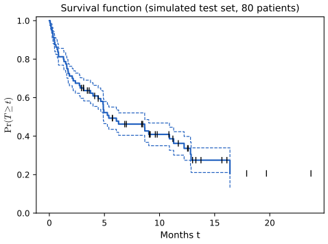
fig_18_12, kaplan_meier. Reproduces Hastie, Tibshirani and Friedman (2009), Figure 18.12 (on simulated data). Download: PDF · SVGThe conceptual model (the book's Figure 18.13) has two cell types; patients with the good type live longer on average, with much overlap. Survival time is then a noisy surrogate for cell type, and a fully supervised method weights the genes most related to survival, which are only partly related to cell type. If we could instead estimate the cell type from the many genes that express it together, we might predict better. Principal components find combinations with large variance, but the leading component of all genes need not relate to survival. Supervised principal components restricts attention to genes that are individually related to the outcome.
Algorithm 18.1 (supervised principal components) p. 678
- Compute the standardised univariate regression coefficient of the outcome on each feature.
- For each threshold \(\theta\) in a list \(0\le\theta_1<\dots<\theta_K\):
- keep the features whose coefficient exceeds \(\theta\) in absolute value, and compute the first \(m\) principal components of this reduced matrix;
- use these components in a regression model to predict the outcome.
- Choose \(\theta\) (and \(m\)) by cross-validation.
For a quantitative outcome, steps 1 and 2b are least squares; for survival, the Cox score test and the Cox model (Bair et al., 2006).
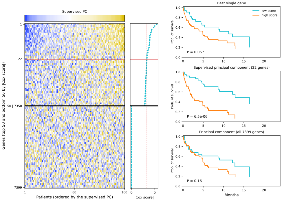
fig_18_14, survival_spc. Reproduces Hastie, Tibshirani and Friedman (2009), Figure 18.14 (on simulated data). Download: PDF · SVGIn the book, the cross-validated Cox-score cutoff 3.53 keeps 27 genes, the supervised component is significant on the test data (likelihood-ratio \(p=0.005\); dichotomised, log-rank \(p=0.006\)), while the best single gene (\(p=0.15\)) and the first principal component of all genes (\(p=0.14\)) are not. The simulation shows the same contrast, more sharply because the model holds exactly. More than one component is allowed, but supervision tends to align the first component with the outcome, and the mathematics below uses one.
18.6.1 Connection to Latent-Variable Modeling
pp. 678–679 Suppose the response depends on a latent variable \(U\),
\[ Y=\beta_0+\beta_1U+\varepsilon, \tag{18.32} \]and a set \(\mathcal P\) of features (a pathway) measures it with noise,
\[ X_j=\alpha_{0j}+\alpha_{1j}U+\epsilon_j,\quad j\in\mathcal P, \tag{18.33} \]with mean-zero errors independent of everything else; the other features are independent of \(U\). This is a single-factor model (Mardia et al., 1979; Section 14.7). Supervised principal components estimates \(\mathcal P\) by screening (a feature's univariate coefficient has non-zero mean only if \(\alpha_{1j}\ne0\)), estimates \(U\) by the leading principal component of the screened features, and estimates (18.32) by the final regression.
See also (companion course): Bayesian and Probabilistic Machine Learning, Section 12.2.1, maximum-likelihood probabilistic PCA.
Result 18.10 (the leading principal component estimates the factor) pp. 679–680, (18.35)
(a) In model (18.33) restricted to \(j\in\mathcal P\), with \(U\sim N(0,1)\) and Gaussian errors of a common variance \(\sigma^2\), the maximum-likelihood estimate of the loading vector \(\alpha_1\) is proportional to the leading eigenvector of the sample covariance of \(X_{\mathcal P}\) (probabilistic PCA with one component), and the best linear predictor of \(U\) from \(X_{\mathcal P}\) is proportional to the leading principal component score. (b) The leading principal component \(\hat u=\bX_{\mathcal P}v_1/d\) of the centred \(N\times|\mathcal P|\) matrix \(\bX_{\mathcal P}\) satisfies the self-consistency equation
\[ \hat u=\frac1{d^2}\sum_{j\in\mathcal P}\langle\hat u,x_j\rangle x_j, \tag{18.35} \]where \(x_j\) are the columns and \(d\) the leading singular value: \(\hat u\) is a weighted average of the features with weights given by their own inner products with \(\hat u\).
Proof
(a) Marginally
\[ X_{\mathcal P}\sim N(\alpha_0,\alpha_1\alpha_1^\T+\sigma^2\bI). \]The log-likelihood depends on the data through the sample covariance \(\bS\): \(-\frac N2[\log\det\bSig+\Tr(\bSig^{-1}\bS)]\). For \(\bSig=aa^\T+\sigma^2\bI\), Tipping and Bishop (1999) show that the maximiser has \(a\) along the leading eigenvector of \(\bS\) with \(\|a\|^2=\ell_1-\hat\sigma^2\) (\(\ell_1\) the largest eigenvalue) and \(\hat\sigma^2\) the mean of the other eigenvalues; the companion course proves this in full. Given \(X\),
\[ \E(U\given X)=a^\T(aa^\T+\sigma^2\bI)^{-1}(X-\alpha_0)=a^\T(X-\alpha_0)/(\|a\|^2+\sigma^2) \](Sherman–Morrison), proportional to the projection on the leading eigenvector, i.e. the first principal component score. (b) With \(\bX_{\mathcal P}=\bU\bD\bV^\T\), \(\hat u=u_1\) satisfies \(\bX_{\mathcal P}\bX_{\mathcal P}^\T\hat u=d^2\hat u\). Since \(\bX_{\mathcal P}\bX_{\mathcal P}^\T=\sum_jx_jx_j^\T\), this is \(\sum_j\langle x_j,\hat u\rangle x_j=d^2\hat u\), which is (18.35). ∎
If \(p\) and \(p_1=|\mathcal P|\) grow with \(p_1\) small relative to \(p\), the leading supervised component is consistent for the latent factor under reasonable conditions, while the ordinary leading component may be swamped by noise features (Bair et al., 2006). If the screening keeps many features, pre-conditioning (Section 18.6.3) finds a smaller set.
18.6.2 Relationship with Partial Least Squares
pp. 680–681 Partial least squares (Section 3.5.2) downweights noisy features but keeps them, and many noisy features contaminate it; Bair et al. (2006) found that throwing them away is the key to supervised principal components. Thresholded PLS applies PLS to the screened features. With standardised features its first variate is
\[ z=\sum_{j\in\mathcal P}\langle y,x_j\rangle x_j, \tag{18.34} \]whereas the supervised component satisfies (18.35). PLS weights each feature by its inner product with the noisy outcome \(y\); supervised principal components uses the "self-consistent" weights \(\langle\hat u,x_j\rangle\), averaged over many features, which should be less noisy. If \(N,p,p_1\to\infty\) with \(p_1/N\to0\), the techniques of Bair et al. (2006) give
\[ z=u+O_p(1),\qquad \hat u=u+O_p\big(\sqrt{p_1/N}\big), \tag{18.36} \]with \(u\) the true latent variable (up to scaling).
See also (this course): Result 3.22, properties of PLS, and the principal components regression and PLS demo.
Filling the gap 18.7: why PLS has an error floor and supervised PCs do not (a heuristic for (18.36)) p. 680
Derivation
Take centred vectors in \(\R^N\): \(x_j=\alpha_ju+e_j\) for \(j\in\mathcal P\), with \(\|u\|^2=N\) and independent noise vectors \(e_j\) with \(\E e_je_j^\T=\bI\), and \(y=\beta u+\varepsilon\). PLS. The weights are \(w_j=\langle y,x_j\rangle=\alpha_j\beta N+\nu_j\) with
\[ \nu_j=\alpha_j\langle\varepsilon,u\rangle+\beta\langle u,e_j\rangle+\langle\varepsilon,e_j\rangle, \]and
\[ z=\Big(\sum_jw_j\alpha_j\Big)u+\sum_jw_je_j. \]The coefficient of \(u\) is about \(\beta N\|\alpha\|^2\), of order \(Np_1\). In the noise term, \(\sum_j\langle\varepsilon,e_j\rangle e_j\) has conditional mean \(\sum_j\E(e_je_j^\T)\varepsilon=p_1\varepsilon\): a copy of the outcome noise, multiplied by \(p_1\), grows exactly like the signal. Divided by the signal coefficient it leaves \(\varepsilon/(\beta N\bar{\alpha^2})\) in every coordinate, whatever \(p_1\) is; the other noise terms are sums of \(p_1\) independent pieces and shrink relative to the signal like \(1/\sqrt{p_1}\). So \(z\) estimates \(u\) with an error that does not go away as more features are averaged: one noisy outcome is all PLS has to weight them. Supervised PC. \(\hat u\) is the leading eigenvector of
\[ \sum_jx_jx_j^\T=\|\alpha\|^2uu^\T+\sum_je_je_j^\T+\text{cross terms}, \]which does not involve \(y\) at all. The mean \(p_1\bI\) of the noise part does not move eigenvectors, and its fluctuation and the cross terms have operator norm of order \(\sqrt{p_1N}+N\), small against the signal eigenvalue \(\|\alpha\|^2N\asymp p_1N\) when \(p_1\) is large; by eigenvector perturbation (Davis–Kahan), the angle between \(\hat u\) and \(u\) tends to zero as \(p_1\) grows. That is the content of (18.36): no floor for \(\hat u\), a floor for \(z\). The precise rates, under the book's normalisation, are in Bair et al. (2006).
Numerically (\(N=100\), loadings 0.5, \(\beta=1\), noise sd 1.5, standardised features, 50 replications), \(1-|\mathrm{corr}|\) with \(u\) is 0.157 and 0.157 for \(z\) and \(\hat u\) with \(p_1=10\); 0.042 and 0.040 with 50; 0.013 and 0.010 with 200; 0.0044 and 0.0020 with 1000: the supervised component keeps improving at the full rate, PLS levels off. ∎
The book compares the methods on a simulation with \(N=100\) and \(p=5000\):
\[ x_{ij}=\begin{cases}3+\epsilon_{ij}&i\le50,\\4+\epsilon_{ij}&i>50,\end{cases}\quad j=1,\dots,50;\qquad x_{ij}=\begin{cases}1.5+\epsilon_{ij}&1\le i\le25\text{ or }51\le i\le75,\\5.5+\epsilon_{ij}&26\le i\le50\text{ or }76\le i\le100,\end{cases}\quad j=51,\dots,250; \] \[ x_{ij}=\epsilon_{ij},\quad j=251,\dots,5000;\qquad y_i=2\cdot\frac1{50}\sum_{j=1}^{50}x_{ij}+\varepsilon_i, \tag{18.37} \]with independent \(\epsilon_{ij}\sim N(0,1)\) and \(\varepsilon_i\sim N(0,1.5^2)\). The first 50 genes differ by one unit between samples 1–50 and 51–100, and this difference drives \(y\); the next 200 differ by four units between two other groups, unrelated to \(y\); the rest are noise.
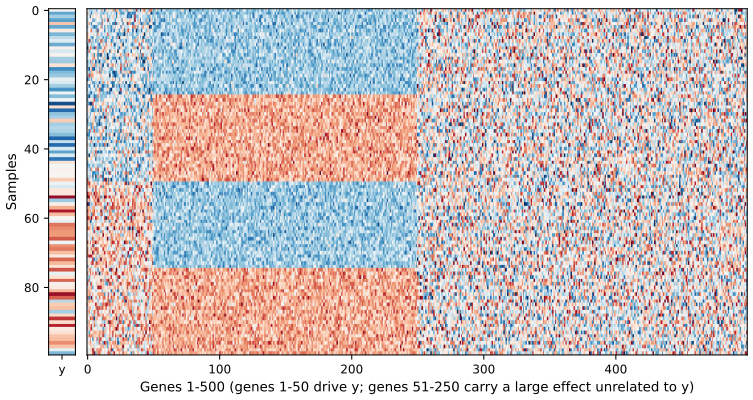
fig_18_15. Reproduces Hastie, Tibshirani and Friedman (2009), Figure 18.15. Download: PDF · SVG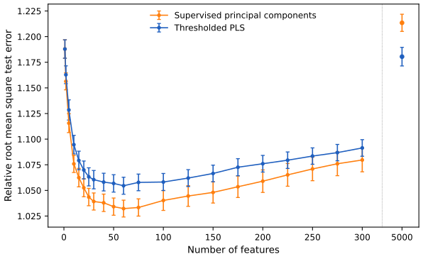
fig_18_16, spc_study. Reproduces Hastie, Tibshirani and Friedman (2009), Figure 18.16. Download: PDF · SVG18.6.3 Pre-Conditioning for Feature Selection
pp. 681–683 Supervised principal components predicts well but does not give a sparse model, and the kept features can be redundant. The lasso is sparse but suffers from the many noise features. Pre-conditioning (Paul et al., 2008) first computes the supervised-PC prediction \(\hat y_i\) on the training set (threshold by cross-validation), then runs the lasso with \(\hat y_i\) in place of \(y_i\), on all features. The denoised outcome makes the lasso less prone to overfitting; its tuning parameter is chosen on grounds such as parsimony.
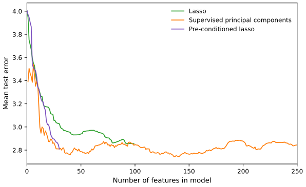
fig_18_17, precondition_example. Reproduces Hastie, Tibshirani and Friedman (2009), Figure 18.17. Download: PDF · SVGPre-conditioning works with other initial estimates and other post-processors than the lasso (Paul et al., 2008).
18.7 Feature Assessment and the Multiple-Testing Problem
pp. 683–687 Often the goal is not prediction but finding the features that differ between groups: proteins whose abundance differs between normal and cancer samples, genes that respond to a treatment. This is multiple hypothesis testing. From here on \(M\) denotes the number of features. The example (Rieger et al., 2004; the book's Table 18.4) has the expression of \(M=12{,}625\) genes in 58 patients: 44 with a normal reaction to radiation therapy and 14 with a severe reaction. For each gene the two-sample \(t\)-statistic is
\[ t_j=\frac{\bar x_{2j}-\bar x_{1j}}{\mathrm{se}_j}, \tag{18.38} \]with \(\bar x_{\ell j}=\sum_{i\in C_\ell}x_{ij}/N_\ell\) (group 1 normal, group 2 sensitive) and the pooled standard error
\[ \mathrm{se}_j=\hat\sigma_j\sqrt{\frac1{N_1}+\frac1{N_2}};\qquad \hat\sigma_j^2=\frac1{N_1+N_2-2}\Big(\sum_{i\in C_1}(x_{ij}-\bar x_{1j})^2+\sum_{i\in C_2}(x_{ij}-\bar x_{2j})^2\Big). \tag{18.39} \]See also (companion course): Statistical Methods for Modern Biology, Section 6.5, the t-test, Result 6.3 (its null distribution) and Section 6.7, multiple testing.
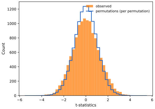
fig_18_18, radsens_permutations. Reproduces Hastie, Tibshirani and Friedman (2009), Figure 18.18. Download: PDF · SVG1189 genes have \(|t_j|\ge2\). If the genes were independent and all null, the number of \(|t_j|\ge2\) would be about binomial with mean \(12{,}625\times0.05=631.3\) and standard deviation 24.5, so 1189 is far out of range (Gap 18.8). Instead of the \(t_{56}\) distribution, which assumes Gaussian data, one can use the permutation distribution: with all \(K=\binom{58}{14}\approx10^{13}\) relabellings (in practice a random sample of \(K=1000\)) and \(t^k_j\) the statistic of gene \(j\) in relabelling \(k\),
\[ p_j=\frac1K\sum_{k=1}^KI(|t_j^k|>|t_j|). \tag{18.40} \]When the genes are on comparable scales, pooling all genes gives a finer null distribution:
\[ p_j=\frac1{MK}\sum_{j'=1}^M\sum_{k=1}^KI(|t_{j'}^k|>|t_j|). \tag{18.41} \]Filling the gap 18.8: the binomial calculation, and what permutation p-values assume pp. 685–686
Derivation
Binomial. If the \(M\) tests are independent, each null gene has \(|t_j|\ge2\) with probability about \(\alpha=0.05\) (for \(t_{56}\) the exact tail is 0.050), so the count is \(\mathrm{Bin}(M,\alpha)\) with mean \(M\alpha=631.25\) and standard deviation \(\sqrt{M\alpha(1-\alpha)}=\sqrt{599.7}=24.5\). The observed 1189 is \((1189-631)/24.5\approx23\) standard deviations above. Correlation between genes inflates the variance of the count but not its mean, so the conclusion that some genes are non-null survives; the permutation average of 633 confirms the null mean without independence. Permutations. Under the null hypothesis that the 58 expression vectors are exchangeable between the groups, every relabelling with 14 sensitive patients is equally likely, so \(t_j\) is a uniform draw from the set of all \(\binom{58}{14}\) relabelled values and (18.40) with all relabellings is an exact p-value (up to ties; companion Result 6.4). With \(K\) random relabellings it is a Monte Carlo approximation. The pooled version (18.41) further assumes that all genes share the same null distribution of \(t\), plausible for a \(t\)-statistic, which is scale free. ∎
Each null hypothesis \(H_{0j}\), "the treatment has no effect on gene \(j\)", is tested against \(H_{1j}\), "it has an effect",
\[ H_{0j}=\text{treatment has no effect on gene }j\quad\text{versus}\quad H_{1j}=\text{treatment has an effect on gene }j, \tag{18.42} \]for \(j=1,\dots,M\), rejecting at level \(\alpha\) when \(p_j<\alpha\). With many tests one needs an overall error measure. Let \(A_j\) be the event that \(H_{0j}\) is falsely rejected, so \(\Pr(A_j)=\alpha\). The family-wise error rate (FWER) is \(\Pr(A)\), \(A=\bigcup_jA_j\): the probability of at least one false rejection. For independent tests it is \(1-(1-\alpha)^M\), close to 1 for large \(M\).
Note on the book: positive dependence and the FWER
The book says that if the tests have positive dependence, meaning \(\Pr(A_j\given A_k)>\Pr(A_j)\), then the FWER is less than \(1-(1-\alpha)^M\). For \(M=2\) this is right:
\[ \Pr(A_1\cup A_2)=2\alpha-\Pr(A_1\cap A_2)<2\alpha-\alpha^2. \]For \(M\ge3\) pairwise positive dependence is not enough. Counterexample with \(M=3\), \(\alpha=0.05\): let all three false rejections happen together with probability \(t=0.0026\), each happen alone with probability \(\alpha-t\), and no other combination occur. Then \(\Pr(A_j)=\alpha\), \(\Pr(A_j\given A_k)=t/\alpha=0.052>\alpha\) for every pair, but \(\Pr(A)=3\alpha-2t=0.1448\), which exceeds \(1-0.95^3=0.1426\). (Uniform p-values with exactly these rejection events exist: put \(p_j\) uniform on \([0,\alpha)\) on \(A_j\) and uniform on \([\alpha,1]\) off it.) The bound does hold under stronger notions such as positive orthant dependence, \(\Pr(\bigcap_jA_j^c)\ge\prod_j\Pr(A_j^c)\), which is Šidák's inequality for two-sided tests of jointly Gaussian statistics.
The Bonferroni method rejects \(H_{0j}\) when \(p_j<\alpha/M\).
Result 18.11 (Bonferroni controls the FWER) p. 686; Exercise 18.16
Under any dependence, the Bonferroni rule has \(\FWER\le M_0\alpha/M\le\alpha\), where \(M_0\) is the number of true nulls. For independent tests,
\[ \FWER=1-(1-\alpha/M)^{M_0}\approx1-e^{-\alpha M_0/M}\approx\alpha M_0/M. \]Proof
By the union bound,
\[ \Pr(\bigcup_{j\in\text{nulls}}A_j)\le\sum_{j\in\text{nulls}}\Pr(p_j<\alpha/M)\le M_0\alpha/M, \]using only that a null p-value satisfies \(\Pr(p_j<u)\le u\). Under independence the complement is the intersection of independent events of probability \(1-\alpha/M\). Finally \((1-\alpha/M)^{M}\to e^{-\alpha}\) and \(1-e^{-\alpha}=\alpha-\alpha^2/2+\dots\approx\alpha\). ∎ The companion course gives the same result with Šidák's exact level: Result 6.5.
For large \(M\) Bonferroni is too conservative: at \(\alpha=0.05\) the threshold is \(0.05/12{,}625=3.96\times10^{-6}\), and no gene reaches it (the smallest pooled permutation p-value is \(4.5\times10^{-6}\)). Refinements adjust p-values without independence (Dudoit et al., 2002b).
18.7.1 The False Discovery Rate
pp. 687–690 The outcomes of \(M\) tests are summarised in the book's Table 18.5:
| Called not significant | Called significant | Total | |
|---|---|---|---|
| \(H_0\) true | \(U\) | \(V\) | \(M_0\) |
| \(H_0\) false | \(T\) | \(S\) | \(M_1\) |
| Total | \(M-R\) | \(R\) | \(M\) |
\(V\) is the number of false positives; the FWER is \(\Pr(V\ge1)\), the type I error rate \(\E(V)/M_0\), the type II error rate \(\E(T)/M_1\) and the power \(1-\E(T)/M_1\). The false discovery rate is
\[ \FDR=\E(V/R), \tag{18.43} \]with \(V/R=0\) when \(R=0\): the expected proportion of false positives among the features called significant (Benjamini and Hochberg, 1995).
Algorithm 18.2 (Benjamini–Hochberg) p. 688
- Fix the false discovery rate \(\alpha\) and let \(p_{(1)}\le p_{(2)}\le\dots\le p_{(M)}\) be the ordered p-values.
- Define \[ L=\max\Big\{j:\ p_{(j)}<\alpha\cdot\frac jM\Big\}. \tag{18.44} \]
- Reject all \(H_{0j}\) with \(p_j\le p_{(L)}\), the BH rejection threshold.
Result 18.12 (BH controls the FDR) p. 687, (18.45); Benjamini and Hochberg (1995)
If the null p-values are independent of each other and of the non-null p-values, and each null p-value is uniform on \([0,1]\), then whatever the distribution of the non-null p-values,
\[ \FDR\le\frac{M_0}M\alpha\le\alpha. \tag{18.45} \]Proof (short)
Write
\[ V/R=\sum_{j\in\mathcal H_0}I(H_{0j}\text{ rejected})/\max(R,1), \]so
\[ \FDR=\sum_{j\in\mathcal H_0}\E[I(\text{reject }j)/\max(R,1)], \]and it suffices to show that each null term is at most \(\alpha/M\). Fix a null \(j\). Let \(R^{(j)}\) be the number of rejections that BH would make if \(p_j\) were replaced by 0; it depends only on the other p-values. Claim: on the event that \(H_{0j}\) is rejected, \(R=R^{(j)}\), and \(H_{0j}\) is rejected exactly when \(p_j<\alpha R^{(j)}/M\) (up to the boundary, which has probability zero). Indeed BH rejects the \(R\) smallest p-values with \(R=\max\{k:p_{(k)}<\alpha k/M\}\); if \(p_j\) is among them, lowering it to 0 does not change which \(k\) satisfy the condition (the order statistics at and above position \(R\) are unchanged), so \(R=R^{(j)}\); and \(p_j\) is rejected iff \(p_j\le p_{(R)}<\alpha R/M\), while conversely if \(p_j<\alpha R^{(j)}/M\) then raising \(p_j\) from 0 to its value keeps at least \(R^{(j)}\) p-values below \(\alpha R^{(j)}/M\), so \(R\ge R^{(j)}\) and \(p_j\) is rejected. Hence, conditioning on the other p-values (independent of \(p_j\)),
\[ \E\Big[\frac{I(\text{reject }j)}{\max(R,1)}\Big]=\E\Big[\frac{I(p_j<\alpha R^{(j)}/M)}{R^{(j)}}\Big]=\E\Big[\frac{\alpha R^{(j)}/M}{R^{(j)}}\Big]=\frac\alpha M, \]because \(p_j\) is uniform and \(R^{(j)}\ge1\). Summing over the \(M_0\) nulls gives \(\FDR=M_0\alpha/M\) (equality with continuous uniform nulls). ∎ The companion course gives this proof in full detail, with the step-up formulation: Statistical Methods for Modern Biology, Result 6.6; its FDR control demo checks the bound by simulation.
With dependent tests BH still controls the FDR under positive regression dependence (Benjamini and Yekutieli, 2001), and \(\alpha\sum_{k\le M}1/k\) replaces \(\alpha\) under arbitrary dependence. For illustration the book takes \(\alpha=0.15\).
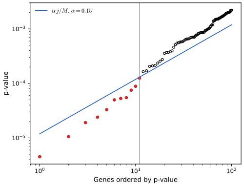
fig_18_19, bh. Reproduces Hastie, Tibshirani and Friedman (2009), Figure 18.19. Download: PDF · SVGA more direct route fixes a cut-point and estimates the FDR of the resulting rule from the permutations.
Algorithm 18.3 (plug-in estimate of the FDR) p. 689
- Create \(K\) permutations of the data, giving statistics \(t_j^k\), \(j=1,\dots,M\), \(k=1,\dots,K\).
- For a range of cut-points \(C\), let \[ R_{\rm obs}=\sum_{j=1}^MI(|t_j|>C),\qquad \widehat{\E(V)}=\frac1K\sum_{j=1}^M\sum_{k=1}^KI(|t_j^k|>C). \tag{18.46} \]
- Estimate the FDR by \(\hFDR=\widehat{\E(V)}/R_{\rm obs}\).
At the cut-point 4.101: 11 observed \(|t_j|\) reach it, and 1579 of the \(12{,}625\times1000\) permuted values do (book: 1518; the permutations are random), 1.579 per permutation, so \(\hFDR=1.579/11=0.144\), close to the \(\alpha=0.15\) used by BH. This is not a coincidence.
Result 18.13 (BH is the plug-in rule) p. 689; Exercise 18.17
With the pooled permutation p-values (18.41), let \(\hFDR_{(j)}\) be the plug-in estimate at the cut-point \(|t|_{(j)}\), the \(j\)-th largest observed \(|t|\), counting \(|t|\ge|t|_{(j)}\) as rejected. Then \(\hFDR_{(j)}=p_{(j)}M/j\), and BH at level \(\alpha\) rejects exactly the \(L=\max\{j:\hFDR_{(j)}<\alpha\}\) genes with the largest \(|t|\). In particular \(\hFDR\) at the BH cut-point is below \(\alpha\), and at the next cut-point \(|t|_{(L+1)}\) it is at least \(\alpha\).
Proof
With no ties, the gene with the \(j\)-th largest \(|t|\) has the \(j\)-th smallest pooled p-value \(p_{(j)}=\#\{(j',k):|t^k_{j'}|>|t|_{(j)}\}/(MK)\). Rejecting \(|t|\ge|t|_{(j)}\) gives \(R_{\rm obs}=j\) and
\[ \widehat{\E(V)}=\#\{(j',k):|t^k_{j'}|>|t|_{(j)}\}/K=Mp_{(j)} \](strict inequality in the permutation count, as in (18.41)). So \(\hFDR_{(j)}=Mp_{(j)}/j\), and \(p_{(j)}<\alpha j/M\iff\hFDR_{(j)}<\alpha\). (18.44) takes the largest such \(j\). For \(j=L+1\) the BH condition fails, i.e. \(\hFDR_{(L+1)}\ge\alpha\). ∎ On the radiation data, for \(\alpha=0.05,0.10,0.15,0.20,0.25,0.30\), BH rejects 0, 8, 11, 19, 64 and 119 genes, and the largest plug-in rule with \(\hFDR<\alpha\) gives the same numbers (Exercise 18.19).
The plug-in estimate rests on the approximation
\[ \E(V/R)\approx\frac{\E(V)}{\E(R)}, \tag{18.47} \]and is consistent (Storey, 2002; Storey et al., 2004). Its numerator estimates \((M/M_0)\E(V)\), because the permutations treat all \(M\) genes as null; with an estimate \(\hat M_0\) the better estimate is \((\hat M_0/M)\hFDR\), and equivalently BH can be run at level \(\alpha M/\hat M_0\) (by (18.45)). Exercise 18.19 estimates \(M_0\). An FDR of 0.15 is not a type I error: it is the expected proportion of false leads in the list handed to the scientist, which can be acceptable in exploratory work.
Filling the gap 18.9: why the permutation numerator estimates \((M/M_0)\E(V)\) pp. 689–690
Derivation
For a fixed cut-point \(C\), \(\E(V)=\sum_{j\in\mathcal H_0}\Pr(|t_j|>C)=M_0\,q(C)\) if every null statistic has the same tail probability \(q(C)\). Each permuted statistic \(t_j^k\), null or not in reality, is a draw from (approximately) the null distribution, so
\[ \E\,\widehat{\E(V)}=\frac1K\sum_j\sum_k\Pr(|t^k_j|>C)=Mq(C)=(M/M_0)\E(V). \]The plug-in estimate is therefore biased upward by the factor \(M/M_0\ge1\), i.e. conservative, and multiplying it by \(\hat M_0/M\) removes the bias when \(\hat M_0\) is accurate. ∎
18.7.2 Asymmetric Cutpoints and the SAM Procedure
pp. 690–692 Using \(|t_j|\) treats both directions alike. If most changes go one way, separate cut-points for the two tails are better. SAM (significance analysis of microarrays) plots the ordered statistics \(t_{(1)}\le\dots\le t_{(M)}\) against the expected order statistics \(\tilde t_{(j)}=\frac1K\sum_kt^k_{(j)}\), the averages of the ordered statistics of each permutation. Two lines parallel to the 45° line at distance \(\Delta\) define a band. Moving right from the origin, the first gene to leave the band above defines the upper cut-point \(C_{\rm hi}\), and every gene beyond it is called; likewise \(C_{\rm low}\) on the left. The FDR of the pair is estimated by the plug-in rule, and \(\Delta\) is chosen by inspecting the trade-off.
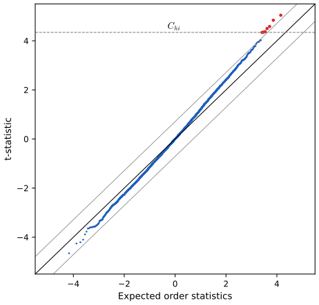
fig_18_20, sam_cutpoints. Reproduces Hastie, Tibshirani and Friedman (2009), Figure 18.20. Download: PDF · SVGThere is an analogy with likelihood-ratio tests, which reject when
\[ \ell(t_j)-\ell_0(t_j)>\Delta \tag{18.48} \]for log-likelihoods under the alternative and the null; depending on the two likelihoods the threshold for \(t_j\) differs from that for \(-t_j\). SAM rejects when
\[ |t_{(j)}-\tilde t_{(j)}|>\Delta, \tag{18.49} \]with a threshold depending on the null value \(\tilde t_{(j)}\) (strictly, SAM calls every gene beyond the first exceedance, so it is a monotone version of (18.49)).
18.7.3 A Bayesian Interpretation of the FDR
pp. 692–693 The positive false discovery rate conditions on at least one rejection:
\[ \pFDR=\E\Big[\frac VR\,\Big|\,R>0\Big]. \tag{18.50} \](The book remarks that the FDR is undefined when \(\Pr(R=0)>0\); with the convention \(V/R=0\) for \(R=0\) it is defined, and \(\FDR=\pFDR\cdot\Pr(R>0)\).) Let \(\Gamma\) be the rejection region of a single test, e.g. \((-\infty,-4.10)\cup(4.10,\infty)\) (the book prints \(\{-(\infty,-2)\cup(2,\infty)\}\) on p. 693, with a stray minus sign). Suppose \(M\) identical tests with i.i.d. pairs \((t_j,Z_j)\), \(Z_j=0\) if the \(j\)-th null is true and 1 otherwise, with
\[ t_j\given Z_j\sim(1-Z_j)\cdot F_0+Z_j\cdot F_1, \tag{18.51} \]and \(\Pr(Z_j=0)=\pi_0\), so that marginally
\[ t_j\sim\pi_0\cdot F_0+(1-\pi_0)\cdot F_1. \tag{18.52} \]Result 18.14 (the pFDR is a posterior probability) p. 693, (18.53); Exercises 18.18 and 18.20
Under (18.51)–(18.52), for every \(M\),
\[ \pFDR(\Gamma)=\Pr(Z_j=0\given t_j\in\Gamma)=\frac{\pi_0\Pr_{F_0}(\Gamma)}{\pi_0\Pr_{F_0}(\Gamma)+(1-\pi_0)\Pr_{F_1}(\Gamma)}. \tag{18.53} \]Proof
Let \(\pi=\Pr(Z_j=0\given t_j\in\Gamma)\), the same for all \(j\). Given \(R=k\ge1\), i.e. given which \(k\) statistics fell in \(\Gamma\), the indicators \(Z_j\) of those \(k\) are independent (the pairs are i.i.d.) and each is 0 with probability \(\pi\), since conditioning on the other pairs does not affect pair \(j\). So \(V\given R=k\sim\mathrm{Bin}(k,\pi)\) and \(\E[V/R\given R=k]=k\pi/k=\pi\). Then
\[ \pFDR=\sum_{k=1}^M\E\Big[\frac VR\,\Big|\,R=k\Big]\Pr(R=k\given R>0)=\pi\sum_{k=1}^M\Pr(R=k\given R>0)=\pi. \]The second expression is Bayes' theorem: \(\Pr(Z=0,t\in\Gamma)=\pi_0\Pr_{F_0}(\Gamma)\) and
\[ \Pr(t\in\Gamma)=\pi_0\Pr_{F_0}(\Gamma)+(1-\pi_0)\Pr_{F_1}(\Gamma); \]the first probability is the type I error of \(\Gamma\) and the second the power, which is Exercise 18.18's form (18.59). ∎
An FDR describes a whole rejection region, so a gene with \(t_j=5\) and one with \(t_j=2\) inside the same region get the same number. The q-value of \(t_j\) (Storey, 2003) is the smallest FDR over the rejection regions (here, symmetric ones) that reject \(t_j\), so it is smaller for \(t_j=5\). The local false discovery rate (Efron and Tibshirani, 2002) at \(t_0\) is
\[ \Pr(Z_j=0\given t_j=t_0), \tag{18.54} \]the pFDR of an infinitesimal region around \(t_0\); by (18.53) with densities, it is \(\pi_0f_0(t_0)/f(t_0)\).
See also (companion course): Statistical Methods for Modern Biology, Definition 6.3 (the two-groups model) and Result 6.7 (local and tail-area fdr).
Filling the gap 18.10: q-values from BH, and why they are monotone p. 693
Derivation
For nested regions \(\Gamma_c=\{|t|\ge c\}\), the plug-in estimate at \(c=|t_j|\) is \(\hFDR(|t_j|)=Mp_j/\#\{i:p_i\le p_j\}\) (Result 18.13). The q-value takes the smallest estimate among all regions that contain \(t_j\), i.e. all \(c\le|t_j|\): \(q_j=\min_{i:\,p_i\ge p_j}Mp_i/\#\{l:p_l\le p_i\}\). This is the BH-adjusted p-value: \(H_{0j}\) is rejected by BH at level \(\alpha\) iff \(q_j<\alpha\). Taking the minimum over larger regions makes \(q\) non-decreasing in \(p\), while the raw ratio \(Mp_{(j)}/j\) need not be (it can dip when several p-values are close). ∎ See also Filling the gap 6.13 of the companion course.
Bibliographic Notes
pp. 693–694 Dudoit et al. (2002a) compare discrimination methods for gene expression; Bickel and Levina (2004) and Levina (2002) show that diagonal LDA can have lower asymptotic error than full LDA when \(p,N\to\infty\) with \(p>N\). Nearest shrunken centroids: Tibshirani et al. (2001a, 2003); regularised logistic regression: Zhu and Hastie (2004); the fused lasso: Tibshirani et al. (2005); the elastic net: Zou and Hastie (2005); supervised principal components: Bair and Tibshirani (2004), Bair et al. (2006); censored survival data: Kalbfleisch and Prentice (1980). The FDR: Benjamini and Hochberg (1995), with later work by Efron and Tibshirani (2002), Storey (2002), Genovese and Wasserman (2004), Storey and Tibshirani (2003) and Benjamini and Yekutieli (2005); Dudoit et al. (2002b) review methods for differentially expressed genes.
Exercises
All 20 exercises of Chapter 18 (Hastie, Tibshirani and Friedman, 2009, pp. 694–698), restated in my own words, with complete solutions (hidden).
Exercise 18.1. For a coefficient vector \(\hb\), let \(\hb/\|\hb\|_2\) be its normalised version. Show that as \(\lambda\to\infty\) the normalised ridge estimates converge to the normalised one-component partial-least-squares estimates.
Solution
Use centred (and, as for PLS in Section 3.5.2, standardised) inputs and a centred response. By Result 18.6,
\[ \hb_\lambda=(\bX^\T\bX+\lambda\bI)^{-1}\bX^\T\by=\lambda^{-1}(\bI+\bX^\T\bX/\lambda)^{-1}\bX^\T\by. \]For \(\lambda>\|\bX^\T\bX\|\) the Neumann series gives
\[ (\bI+\bX^\T\bX/\lambda)^{-1}=\bI-\bX^\T\bX/\lambda+O(\lambda^{-2}), \]so \(\lambda\hb_\lambda=\bX^\T\by+O(1/\lambda)\) and \(\hb_\lambda/\|\hb_\lambda\|\to\bX^\T\by/\|\bX^\T\by\|\) (assuming \(\bX^\T\by\ne0\)). One-component PLS uses the direction \(\varphi_1=\bX^\T\by\) (the inner products \(\langle x_j,\by\rangle\)), the derived input \(z_1=\bX\varphi_1\), and regresses \(\by\) on it: \(\hat y=\hat\theta_1z_1\), \(\hat\theta_1=\langle z_1,\by\rangle/\langle z_1,z_1\rangle\). In terms of the inputs its coefficient vector is \(\hb^{\rm PLS}=\hat\theta_1\bX^\T\by\), a multiple of \(\bX^\T\by\); since \(\hat\theta_1=\|\bX^\T\by\|^2/\|\bX\bX^\T\by\|^2>0\), its normalised version is \(\bX^\T\by/\|\bX^\T\by\|\), the same limit. (Heavily penalised ridge and one-step PLS both just use the univariate inner products, which is one reason they behave alike when \(p\gg N\).)
Exercise 18.2 (nearest shrunken centroids and the lasso). In a naive Bayes Gaussian model the features are independent within each class, \(x_{ij}\sim N(\mu_j+\mu_{jk},\sigma_j^2)\) for \(i\in C_k\), with \(\sum_k\mu_{jk}=0\). With \(\hat\sigma_j^2=s_j^2\), consider
\[ \min_{\{\mu_j,\mu_{jk}\}}\Big\{\frac12\sum_{j=1}^p\sum_{k=1}^K\sum_{i\in C_k}\frac{(x_{ij}-\mu_j-\mu_{jk})^2}{s_j^2}+\lambda\sqrt{N_k}\sum_{j=1}^p\sum_{k=1}^K\frac{|\mu_{jk}|}{s_j}\Big\}. \tag{18.55} \]Show that the solution is the nearest shrunken centroid estimator (18.5) with \(s_0=0\) and \(m_k^2=1/N_k\) instead of \(1/N_k-1/N\).
Solution
(Read \(\lambda\sqrt{N_k}\) inside the sum over \(k\).) This is Result 18.3: with \(\mu_j=\bar x_j\), each \((j,k)\) term reduces to \(\tfrac12(d_{kj}-\delta)^2+\lambda|\delta|\) in \(\delta=\mu_{jk}/(s_jm_k)\), \(m_k=1/\sqrt{N_k}\), solved by \(\soft(d_{kj},\lambda)\); then \(\hat\mu_j+\hat\mu_{jk}=\bar x_j+s_jm_k\soft(d_{kj},\lambda)\) is (18.7) with \(s_0=0\), \(\Delta=\lambda\). As explained there, if \(\mu_j\) is minimised jointly its optimum is \(\bar x_j-\sum_k(N_k/N)\hat\mu_{jk}\), so the identity is exact only with \(\mu_j\) held at the overall mean (or with the weighted constraint \(\sum_kN_k\mu_{jk}=0\) in place of \(\sum_k\mu_{jk}=0\)). The factor \(1/N_k-1/N\) of NSC comes from the variance of \(\bar x_{kj}-\bar x_j\) (Result 18.2(c)); the lasso form uses the variance \(\sigma^2/N_k\) of \(\bar x_{kj}\) alone, which is what one gets when \(\mu_j\) is treated as known.
Exercise 18.3. Show that the coefficients of the penalised multinomial problem (18.11) satisfy \(\sum_k\hat\beta_{kj}=0\) for every \(j\). What about the intercepts? Discuss the problems with them and how to resolve them.
Solution
This is Result 18.4: shifting all \(\beta_k\) by the same vector leaves the likelihood unchanged and the penalty is minimised when their mean is zero. The intercepts are unpenalised, so the same shift argument shows that the log-likelihood is constant along \(\beta_{k0}\mapsto\beta_{k0}+c\): the maximiser is not unique (a line of solutions), and Newton's method faces a singular Hessian. Remedies: fix \(\beta_{10}=0\) (a reference class), impose \(\sum_k\beta_{k0}=0\), or add a tiny ridge penalty on the intercepts, which picks the solution with \(\sum_k\beta_{k0}=0\). All give the same fitted probabilities. The code fixes \(\beta_{10}=0\).
Exercise 18.4. Derive (18.15). (Use the gradient of the penalised residual sum of squares to show that, for \(\lambda>0\), \(\hb=\bX^\T s\) for some \(s\in\R^N\).)
Solution
The gradient of \(\|\by-\bX\beta\|^2+\lambda\|\beta\|^2\) is \(-2\bX^\T(\by-\bX\beta)+2\lambda\beta\); setting it to zero gives \(\hb=\bX^\T s\) with \(s=(\by-\bX\hb)/\lambda\). Substituting \(\hb=\bX^\T s\) back, \(\lambda s=\by-\bX\bX^\T s\), so \(s=(\bX\bX^\T+\lambda\bI)^{-1}\by\). With \(\bX=\bR\bV^\T\), \(\bX\bX^\T=\bR\bR^\T\) and
\[ \hb=\bV\bR^\T(\bR\bR^\T+\lambda\bI)^{-1}\by=\bV(\bR^\T\bR+\lambda\bI)^{-1}\bR^\T\by, \]using the push-through identity
\[ \bR^\T(\bR\bR^\T+\lambda\bI)^{-1}=(\bR^\T\bR+\lambda\bI)^{-1}\bR^\T \](multiply both sides by \(\bR\bR^\T+\lambda\bI\) on the right and \(\bR^\T\bR+\lambda\bI\) on the left). Full details in Result 18.6.
Exercise 18.5. Prove the theorem (18.16)–(18.17) by decomposing \(\beta\) and the rows of \(\bX\) into their projections onto the column space of \(\bV\) and its orthogonal complement.
Solution
See Result 18.5: the rows of \(\bX\) lie in the column space of \(\bV\) (their complement components are zero), so the fitted values depend only on \(\bV^\T\beta\), while the penalty adds \(\|\beta_\perp\|^2\), which must vanish at the optimum.
Exercise 18.6. Show how the theorem of Section 18.3.5 applies to regularised discriminant analysis (Section 4.3.1 and (18.9)).
Solution
First rescale each feature by \(\hat\sigma_j=\sqrt{\hat\Sigma_{jj}}\): in the new coordinates \(\tilde\bSig(\gamma)=\gamma\tilde\bSig+(1-\gamma)\bI\), a covariance shrunk towards the identity. Let \(\tilde\bX=\bR\bV^\T\) be the reduction of the rescaled data. Every quantity RDA uses lies in the column space of \(\bV\): the centroids \(\tilde\mu_k=\bV\bar r_k\) (averages of rows) and the within-class covariance \(\tilde\bSig=\bV\bS_R\bV^\T\), where \(\bS_R\) is the within-class covariance of the rows \(r_i\). Then
\[ \tilde\bSig(\gamma)=\bV[\gamma\bS_R+(1-\gamma)\bI_N]\bV^\T+(1-\gamma)(\bI-\bV\bV^\T), \]so
\[ \tilde\bSig(\gamma)^{-1}\tilde\mu_k=\bV[\gamma\bS_R+(1-\gamma)\bI_N]^{-1}\bar r_k, \]and for any \(x\) the linear discriminant
\[ \tilde x^\T\tilde\bSig(\gamma)^{-1}\tilde\mu_k-\tfrac12\tilde\mu_k^\T\tilde\bSig(\gamma)^{-1}\tilde\mu_k \]equals the same expression computed with \(r=\bV^\T\tilde x\), \(\bar r_k\) and \(\gamma\bS_R+(1-\gamma)\bI_N\). So RDA on the \(N\)-dimensional rows of \(\bR\), with the same \(\gamma\), gives the same scores. Through optimal scoring this is the theorem itself: LDA is a regression of scored indicators on \(\bX\), RDA a ridge regression of them (with penalty \(\propto\) identity after the rescaling), and (18.16)–(18.17) applies. The code checks the identity on the SRBCT data (
RDAcomputes in the reduced space; Gap 18.3).Exercise 18.7. Linear regression with \(p\gg N\) and \(\rank\bX=N\), \(\bX=\bU\bD\bV^\T=\bR\bV^\T\) with \(\bR\) non-singular. (a) Show that there are infinitely many least-squares solutions, all with zero residuals. (b) Show that the ridge estimate is
\[ \hb_\lambda=\bV(\bR^\T\bR+\lambda\bI)^{-1}\bR^\T\by. \tag{18.56} \](c) Show that at \(\lambda=0\) the solution \(\hb_0=\bV\bD^{-1}\bU^\T\by\) has zero residuals and is the zero-residual solution with the smallest Euclidean norm.
Solution
(a) \(\bX\) is \(N\times p\) with rank \(N\), so its columns span \(\R^N\) and \(\bX\beta=\by\) has a solution; its null space has dimension \(p-N>0\), and adding any null vector gives another solution, so there are infinitely many, all with residual zero and hence all minimising the residual sum of squares. (b) and (c): Result 18.6. (The intercept is handled by centring; then the rank is at most \(N-1\) and the statements hold with \(N-1\).)
Exercise 18.8 (data piling). Two-class LDA is the least-squares regression of a \(\pm1\) response (Exercise 4.2). Let \(p\gg N\). (a) For the linear model \(f(x)=\alpha+\beta^\T x\) fitted to \(Y\in\{-1,+1\}\), use Exercise 18.7 to show that there are infinitely many directions \(\hb\) onto which the data project to exactly two points, one per class (data-piling directions; Ahn and Marron, 2010). (b) Show that the distance between the two points is \(2/\|\hb\|\), so these directions define separating hyperplanes with that margin. (c) Argue that there is a single maximal data-piling direction, with the largest distance, given by \(\hb_0=\bV\bD^{-1}\bU^\T\by=\bX^-\by\).
Solution
Centre the inputs (this absorbs \(\alpha\)), and assume \(\rank\bX_c=N-1\), which holds for continuous data with \(p\ge N-1\). (a) The centred response \(\by_c\) lies in the column space of \(\bX_c\) (both are orthogonal to \(\bone\), and that space is all of \(\bone^\perp\)), so \(\bX_c\beta=\by_c\) has infinitely many solutions \(\hb_0+n\), \(\bX_cn=0\). For each, \(x_i^\T\hb-\bar x^\T\hb=y_i-\bar y\): all class \(+1\) points project to one value and all class \(-1\) points to another. (b) The two values differ by \((1-\bar y)-(-1-\bar y)=2\) in the scale of \(x^\T\hb\); along the unit direction \(\hb/\|\hb\|\) the distance is \(2/\|\hb\|\). The hyperplane through the midpoint, perpendicular to \(\hb\), separates the classes with every point at distance \(1/\|\hb\|\). (c) Any direction \(w\) on which the data pile at two distinct values can be rescaled so the values differ by 2, i.e. so that it solves \(\bX_cw=\by_c\); so the piling directions are exactly the normalised solutions, and the distance \(2/\|w\|\) is largest for the solution of smallest norm, which is unique: \(\hb_0=\bX_c^+\by_c=\bV\bD^{-1}\bU^\T\by_c\) (Result 18.6). (The code's
max_data_pilingchecks that the projections take exactly two values, up to \(10^{-14}\).)Exercise 18.9. Compare the maximal data-piling direction with the optimal separating hyperplane (Section 4.5.2). Which has the wider margin, and why? Use a small simulation.
Solution
Theory. The optimal separating hyperplane maximises the smallest distance of any training point to the hyperplane, over all directions. The data-piling hyperplane of Exercise 18.8 puts every point at distance \(1/\|\hb_0\|\), so its smallest distance is \(1/\|\hb_0\|\), and it is a feasible candidate for the SVM problem: the SVM margin is therefore at least as wide. They coincide exactly when every training point is a support vector, which becomes typical when \(p\gg N\): in high dimensions all points tend to lie on the margin. When \(p\) is only slightly above \(N\), the SVM can ignore the points far from the boundary and do much better, while data piling is forced to collapse every class onto a point, which mostly fits noise (it is the limit of LDA with a vanishing ridge, Exercise 18.10).
Simulation (
exercise_18_9_table; \(N=20\), ten per class, identity covariance, the second class shifted by 0.5 in every coordinate, 50 replications, test sets of 1000):\(p\) data-piling gap \(2/\|\hb_0\|\) SVM margin width ratio (min, max) test error, piling test error, SVM 22 1.30 1.99 1.05, 3.49 0.363 0.251 30 2.20 2.59 1.01, 1.82 0.285 0.216 50 3.86 3.96 1.001, 1.11 0.152 0.132 200 9.04 9.05 1.000, 1.009 0.0080 0.0079 The SVM margin is never smaller, it is much wider just above \(p=N\), and the two rules merge as \(p\) grows.
Exercise 18.10. When \(p\gg N\), LDA is degenerate because the within-class covariance \(\bW\) is singular. A regularised version replaces \(\bW\) by \(\bW+\lambda\bI\), giving
\[ \delta_\lambda(x)=x^\T(\bW+\lambda\bI)^{-1}(\bar x_1-\bar x_{-1}). \]Show that \(\delta_0(x)=\lim_{\lambda\downarrow0}\delta_\lambda(x)\) corresponds to the maximal data-piling direction of Exercise 18.8.
Solution
Let \(\delta=\bar x_1-\bar x_{-1}\) and split it as \(\delta=\delta_W+\delta_\perp\) with \(\delta_W\) in the column space of \(\bW\) and \(\delta_\perp\) in its null space. With \(\bW=\sum_\ell w_\ell e_\ell e_\ell^\T\) (\(w_\ell>0\)),
\[ (\bW+\lambda\bI)^{-1}\delta=\sum_\ell\frac{e_\ell^\T\delta}{w_\ell+\lambda}e_\ell+\frac1\lambda\delta_\perp. \]If \(\delta_\perp\ne0\) (true when \(p\ge N-1\) in general position) the second term dominates: \(\delta_\lambda\) itself diverges, but the direction converges, \(\lambda(\bW+\lambda\bI)^{-1}\delta\to\delta_\perp\), so the limiting rule (up to a positive scale, which does not change the classification) is \(x^\T\delta_\perp\). Now show \(\delta_\perp\propto\hb_0\). The data-piling direction satisfies \((x_i-\bar x_{g_i})^\T\hb_0=0\) for every \(i\) (all points of a class project to one value), i.e. \(\hb_0\perp\) every within-class residual, i.e. \(\hb_0\) lies in the null space of \(\bW\). Also \(\hb_0\) lies in the row space of \(\bX_c\), spanned by the within-class residuals and \(\bar x_k-\bar x\propto\delta\); so \(\hb_0=w+c\delta\) with \(w\in\operatorname{col}\bW\). Projecting onto \(\operatorname{col}\bW\): \(0=w+c\delta_W\), so \(\hb_0=c(\delta-\delta_W)=c\,\delta_\perp\). Hence the limit of regularised LDA is the maximal data-piling classifier; the code confirms that the cosine of the angle between the two directions is 1 to within \(10^{-10}\).
Exercise 18.11. \(N\) pairs \((x_i,y_i)\) with \(y_i\in\{0,1\}\) and \(x_i\in\R\) are separable: \(x_{i'}-x_i\ge C>0\) whenever \(y_i=0\), \(y_{i'}=1\). Show that the maximum-likelihood \(\hat\beta\) of the logistic model \(\operatorname{logit}\Pr(Y=1\given X)=\alpha+\beta X\) is undefined.
Solution
Let \(a=\max\{x_i:y_i=0\}\), \(b=\min\{x_i:y_i=1\}\), so \(b-a\ge C\), and let \(m=(a+b)/2\). Take \(\beta=t>0\), \(\alpha=-tm\). Then \(\alpha+\beta x_i=t(x_i-m)\le-tC/2\) for \(y_i=0\) and \(\ge tC/2\) for \(y_i=1\), so every term of the log-likelihood \(\sum_i[y_i\eta_i-\log(1+e^{\eta_i})]\) is at least \(-\log(1+e^{-tC/2})\), and the log-likelihood tends to 0, its supremum (each term is negative), as \(t\to\infty\). No finite \((\alpha,\beta)\) attains 0, since every term is strictly negative at finite parameters. So the supremum is not attained: the MLE does not exist, and any maximising sequence has \(\beta\to\infty\). With \(p>N\) separability is the rule (note on the book after Section 18.3.3), which is why penalised fits must stop at a positive \(\lambda\).
Exercise 18.12. To choose the ridge parameter by 10-fold cross-validation with the shortcut of Section 18.3.5, show that \(\bX\) needs to be reduced to \(\bR\) only once and the same \(\bR\) used in every fold.
Solution
Let \(\bX=\bR\bV^\T\) on all \(N\) rows. For a fold, the training rows form \(\bX_{-k}=\bR_{-k}\bV^\T\) (the corresponding rows of \(\bR\)), and the held-out rows \(\bX_k=\bR_k\bV^\T\). The proof of Result 18.5 used only two facts: \(\bV\) has orthonormal columns, and every training row is \(\bV\) times its row of \(\bR\). Both hold for \(\bX_{-k}\) with the global \(\bV\) (whose column space contains the training rows, even though it may be larger than their own span). So the fit on the fold is \(\hb^{(-k)}=\bV\hat\theta^{(-k)}\), where \(\hat\theta^{(-k)}\) fits the penalised model on the rows of \(\bR_{-k}\), and the held-out predictions are \(x_i^\T\hb^{(-k)}=r_i^\T\hat\theta^{(-k)}\): only \(\bR\) is needed. Line 6 of Table 18.1 is computed this way (the code also checks fold by fold that the predictions equal those of the full \(p\)-dimensional fit).
Exercise 18.13. The \(p>N\) inputs are given only through \(\bK=\bX\bX^\T\), and a new \(x_0\) through \(k_0=\bX x_0\). With the eigen-decomposition \(\bK=\bU\bD^2\bU^\T\), show that the ridged logistic predictions are \(\hat f_0=k_0^\T\hat\alpha\), where (a) \(\hat\alpha=\bU\bD^{-1}\hat\beta\) and (b) \(\hat\beta\) is the ridged logistic estimate with input matrix \(\bR=\bU\bD\). Argue that the same works for any kernel matrix.
Solution
\(\bK=\bU\bD^2\bU^\T\) is the eigen-decomposition corresponding to the SVD \(\bX=\bU\bD\bV^\T\) (assume \(\bD\) invertible, i.e. \(\rank\bK=N\); otherwise drop the zero eigenvalues). By Result 18.5 the ridged logistic fit on \(\bX\) has \(\beta_X=\bV\hat\beta\), with \(\hat\beta\) the fit on \(\bR=\bU\bD\) (and the same intercept). For a new point, \(x_0^\T\beta_X=x_0^\T\bV\hat\beta\), and \(\bV=\bX^\T\bU\bD^{-1}\), so
\[ x_0^\T\bV\hat\beta=(\bX x_0)^\T\bU\bD^{-1}\hat\beta=k_0^\T\hat\alpha \]with \(\hat\alpha=\bU\bD^{-1}\hat\beta\). Only \(\bK\) and \(k_0\) were used. For a general positive semidefinite kernel, Mercer's theorem gives a feature map with \(K(x,x')=\langle\phi(x),\phi(x')\rangle\); the argument applies verbatim with \(\phi(x_i)\) as inputs (in a possibly infinite-dimensional space the reduction is to the span of the \(\phi(x_i)\), i.e. the representer theorem, Result 5.13), and the fit is the kernel logistic regression (12.31)–(12.32).
Exercise 18.14 (distance-weighted 1-NN). Two classes, \(d_+(x_0)\) and \(d_-(x_0)\) the distances from \(x_0\) to the nearest training point of class \(+1\) and \(-1\), \(N_+\) and \(N_-\) the class sizes, \(N=N_++N_-\). (a) Show that
\[ \delta(x_0)=\log\frac{d_-(x_0)}{d_+(x_0)} \tag{18.57} \]is a nonparametric discriminant function corresponding to 1-NN (hint: \(\hat f_+(x_0)=1/(N_+d_+(x_0))\) estimates the class density). (b) How would you introduce priors \(\pi_+,\pi_-\) different from \(N_+/N,N_-/N\)? (c) How would you generalise to \(K\)-NN?
Solution
(a) The ball of radius \(d_+(x_0)\) around \(x_0\) contains exactly one of the \(N_+\) class-\(+1\) points, so the probability of that ball under the class density is estimated by \(1/N_+\), and dividing by its "size" gives \(\hat f_+(x_0)\propto1/(N_+d_+(x_0)^q)\); the hint takes \(q=1\) (in \(p\) dimensions the volume gives \(q=p\), which only rescales \(\delta\) by \(p\) and changes nothing below). With sample priors, the log posterior odds are
\[ \log\frac{(N_+/N)\hat f_+}{(N_-/N)\hat f_-}=\log\frac{d_-(x_0)}{d_+(x_0)}: \]\(N_+\) and \(N_-\) cancel. The rule \(\delta>0\) is \(d_+<d_-\), exactly 1-NN; \(\delta\) is a continuous score, which is what the ROC curves of Figure 18.9 need. (b) Use
\[ \log\frac{\pi_+\hat f_+}{\pi_-\hat f_-}=\log\frac{d_-}{d_+}+\log\frac{\pi_+N_-}{\pi_-N_+}: \]add that constant (with exponent \(q=p\) on the distances if one takes the density estimate literally). (c) Let \(d_{K,\pm}(x_0)\) be the distance to the \(K\)-th nearest point of each class; the ball then contains \(K\) of \(N_\pm\) points, \(\hat f_\pm\propto K/(N_\pm d_{K,\pm}^p)\), and
\[ \delta_K=p\log(d_{K,-}/d_{K,+})+\log\frac{\pi_+N_-}{\pi_-N_+}. \]Alternatively, take the usual \(K\)-NN vote \(\hat p_+=k_+/K\) among the \(K\) nearest overall and use \(\log(\hat p_+/\hat p_-)\) with a continuity correction.
Exercise 18.15 (kernel PCA). From the eigen-decomposition \((\bI-\bM)\bK(\bI-\bM)=\bU\bD^2\bU^\T\), \(\bM=\bone\bone^\T/N\), the principal-component variables are \(\bZ=\bU\bD\). Given the vector \(k_0\) of inner products of a new \(x_0\) with the \(x_i\), show that the centred projections of \(x_0\) on the principal directions are
\[ z_0=\bD^{-1}\bU^\T(\bI-\bM)\big[k_0-\bK\bone/N\big]. \tag{18.58} \]Solution
Let \(\tilde\bX=(\bI-\bM)\bX=\bU\bD\bV^\T\), so \(\tilde\bX\tilde\bX^\T=(\bI-\bM)\bK(\bI-\bM)\) and the principal directions are the columns of \(\bV=\tilde\bX^\T\bU\bD^{-1}\). The centred new point is \(x_0-\bar x\) with \(\bar x=\bX^\T\bone/N\), and its projections are
\[ z_0=\bV^\T(x_0-\bar x)=\bD^{-1}\bU^\T\tilde\bX(x_0-\bar x)=\bD^{-1}\bU^\T(\bI-\bM)\bX(x_0-\bX^\T\bone/N)=\bD^{-1}\bU^\T(\bI-\bM)(k_0-\bK\bone/N), \]using \(\bX x_0=k_0\) and \(\bX\bX^\T=\bK\). For a training point, \(k_0\) is a column of \(\bK\) and \(z_0\) is the corresponding row of \(\bZ\). (Since \(\bU^\T\bone=0\) for the non-zero eigenvalues, the factor \(\bI-\bM\) can even be dropped.)
kernel_pca_scoresimplements this, and agrees with the SVD of the centred data.Exercise 18.16 (Bonferroni). With null hypotheses \(H_{0j}\), p-values \(p_j\), \(A_j\) the event that \(H_{0j}\) is falsely rejected and \(A=\bigcup_jA_j\), the Bonferroni method rejects when \(p_j<\alpha/M\). (a) Show that \(\Pr(A)\le\alpha\). (b) If the tests are independent, \(\Pr(A)=1-\prod_j\Pr(A_j^c)=1-(1-\alpha/M)^M\); show that \(\Pr(A)\approx\alpha\).
Solution
(a) By induction on the hint, \(\Pr(\bigcup_jA_j)\le\sum_j\Pr(A_j)\le M\cdot\alpha/M=\alpha\) (only nulls can produce false rejections, so the sum has at most \(M_0\le M\) non-zero terms). (b)
\[ \log(1-\alpha/M)^M=M\log(1-\alpha/M)=-\alpha-\alpha^2/(2M)-\dots, \]so \((1-\alpha/M)^M\to e^{-\alpha}\) and \(\Pr(A)\to1-e^{-\alpha}=\alpha-\alpha^2/2+\dots\); for \(\alpha=0.05\) this is 0.0488. In fact \(1-(1-\alpha/M)^M\) lies between \(\alpha-\alpha^2/2\) and \(\alpha\) for every \(M\). See Result 18.11.
Exercise 18.17 (BH and the plug-in method). (a) In the notation of Algorithm 18.2, show that for the threshold \(p_0=p_{(L)}\) a proportion of at most \(p_0\) of the permuted values \(t_j^k\) exceed \(|T|_{(L)}\), the \(L\)-th largest \(|t_j|\); hence the plug-in estimate satisfies \(\hFDR\le p_0M/L<\alpha\). (b) Show that the cut-point \(|T|_{(L+1)}\) gives an estimated FDR of at least \(\alpha\).
Solution
(a) With the pooled p-values (18.41), \(p_0=p_{(L)}\) is exactly the proportion of the \(MK\) permuted values that exceed \(|T|_{(L)}\). The plug-in rule at that cut-point has \(R_{\rm obs}=L\) and \(\widehat{\E(V)}=MKp_0/K=Mp_0\), so \(\hFDR=Mp_0/L\), and the BH condition \(p_{(L)}<\alpha L/M\) says \(\hFDR<\alpha\). (The book writes "\(=\alpha\)"; it is a strict inequality.) With per-gene p-values (18.40) the proportion is an average of the per-gene proportions, which is why the book says "at most". (b) \(L\) is the largest index with \(p_{(j)}<\alpha j/M\), so \(p_{(L+1)}\ge\alpha(L+1)/M\), i.e. \(\hFDR\) at the cut-point \(|T|_{(L+1)}\) is \(Mp_{(L+1)}/(L+1)\ge\alpha\). (More precisely BH takes the last crossing: every \(j>L\) has \(\hFDR_{(j)}\ge\alpha\).) See Result 18.13.
Exercise 18.18. Use (18.53) to show
\[ \pFDR=\frac{\pi_0\cdot\{\text{Type I error of }\Gamma\}}{\pi_0\cdot\{\text{Type I error of }\Gamma\}+\pi_1\{\text{Power of }\Gamma\}} \tag{18.59} \](Storey, 2003).
Solution
By Bayes' theorem,
\[ \Pr(Z=0\given t\in\Gamma)=\Pr(t\in\Gamma\given Z=0)\Pr(Z=0)/\Pr(t\in\Gamma), \]with \(\Pr(t\in\Gamma\given Z=0)=\Pr_{F_0}(\Gamma)\), the type I error of the region, \(\Pr(t\in\Gamma\given Z=1)=\Pr_{F_1}(\Gamma)\), its power, and
\[ \Pr(t\in\Gamma)=\pi_0\Pr_{F_0}(\Gamma)+\pi_1\Pr_{F_1}(\Gamma) \]by total probability, \(\pi_1=1-\pi_0\). Combine with (18.53) (Result 18.14).
Exercise 18.19. On the radiation-sensitivity data of Section 18.7: (a) with symmetric two-sided rejection regions on \(t\), compute the plug-in FDR for several cut-points; (b) run BH at several levels \(\alpha\) and show that the results agree with (a); (c) with \((q_{.25},q_{.75})\) the quartiles of the permuted \(t\)-statistics, let \(\hat\pi_0=\#\{t_j\in(q_{.25},q_{.75})\}/(.5M)\), truncated at 1, multiply the estimates of (a) by \(\hat\pi_0\) and examine them; (d) motivate the estimate in (c).
Solution
Computed by
exercise_18_19with \(K=1000\) permutations. (a) and (c):cut-point \(C\) \(R_{\rm obs}\) \(\widehat{\E(V)}\) \(\hFDR\) \(\hat\pi_0\cdot\hFDR\) 2.0 1189 633.4 0.533 0.463 2.5 438 191.4 0.437 0.380 3.0 157 49.7 0.317 0.275 3.5 52 11.2 0.216 0.188 4.0 13 2.24 0.172 0.150 4.5 4 0.41 0.103 0.090 (b) BH with the pooled p-values rejects 0, 8, 11, 19, 64 and 119 genes at \(\alpha=0.05,0.10,0.15,0.20,0.25,0.30\); the largest set of top-\(|t|\) genes whose plug-in estimate is below \(\alpha\) has exactly the same sizes, as Result 18.13 guarantees. (c) The permuted quartiles are \(-0.678\) and \(0.680\); 5484 of the 12,625 observed \(t_j\) fall between them, so \(\hat\pi_0=5484/6312.5=0.869\): about 13% of the genes are estimated to be non-null, and every FDR estimate drops by 13%. (d) Null statistics follow the permutation distribution, so a fraction \(1/2\) of them fall between its quartiles; non-null statistics are shifted away from zero and rarely fall in the central interval. Hence \(\#\{t_j\in(q_{.25},q_{.75})\}\approx M_0/2+\) (a few non-nulls), and \(\hat\pi_0\) estimates \(\pi_0=M_0/M\) with a small upward bias, i.e. conservatively. Multiplying \(\hFDR\) by it corrects the factor \(M/M_0\) of Gap 18.9. This is Storey's (2002) estimator with the central half of the null distribution as the "null region"; the companion course explains the same idea with p-value histograms (Filling the gap 6.12).
Exercise 18.20 (proof of (18.53); the book's title says "result 18.20"). Write
\[ \pFDR=\E\Big(\frac VR\,\Big|\,R>0\Big) \tag{18.60} \] \[ \phantom{\pFDR}=\sum_{k=1}^M\E\Big[\frac VR\,\Big|\,R=k\Big]\Pr(R=k\given R>0), \tag{18.61} \]and use that, given \(R=k\), \(V\) is binomial with \(k\) trials and success probability \(\Pr(H=0\given T\in\Gamma)\) to complete the proof.
Solution
(18.61) is the law of total expectation over the values \(k=1,\dots,M\) of \(R\) given \(R>0\). Given \(R=k\),
\[ \E[V/R\given R=k]=\E[V\given R=k]/k=k\pi/k=\pi, \]with \(\pi=\Pr(H=0\given T\in\Gamma)\), because \(V\given R=k\) is binomial (the \(k\) rejected tests are i.i.d. draws from the conditional law given rejection). The weights \(\Pr(R=k\given R>0)\) sum to 1, so \(\pFDR=\pi\). The binomial claim is justified in Result 18.14.
Demonstrations for this chapter
Each demonstration runs in the browser and links back to these notes. The ▶ Demo boxes above open them already set to the case under discussion.
| Demonstration | What you can see | Sections and results |
|---|---|---|
| Nearest shrunken centroids | The SRBCT data (2308 genes, 63 training and 20 test samples): move the threshold \(\Delta\) and watch genes drop out, the centroids shrink, and the training, 10-fold cross-validated and test errors change; soft or hard thresholding, with or without \(s_0\); the test-sample probabilities (18.8). Presets: 1 diagonal LDA; 2 \(\Delta=4.34\), 43 genes; 3 too much shrinkage; 4 hard thresholding; 5 no \(s_0\). | 18.2; Results 18.2, 18.3 |
| Ridge regression when \(p\gg N\) | One data set of the Figure 18.1 simulation with \(p\) up to 5000: the relative test error against the degrees of freedom, the Bayes risk, and the same fit by the \(p\times p\) normal equations and by the \(N\times N\) reduction, with their costs. Presets: 1 \(p=20\); 2 \(p=100\); 3 \(p=1000\); 4 the minimum-norm fit; 5 two routes, one fit. | 18.1, 18.3.5; Results 18.1, 18.5, 18.6 |
| Supervised principal components | Model (18.37) with 5000 genes: choose how many genes to keep and how many components, and compare supervised principal components with principal components regression on all genes and with thresholded PLS; see which genes carry the first loading. Presets: 1 50 genes; 2 all genes; 3 all genes, three components; 4 too few genes; 5 300 genes. | 18.6–18.6.2; Result 18.10 |
Related demonstrations: in this course, cross-validation the wrong and the right way after screening thousands of inputs (Chapter 7), shrinkage paths and principal components regression and PLS (Chapter 3); in Statistical Methods for Modern Biology, the FDR control demo (Benjamini–Hochberg by simulation) and the elastic net demo. The Python code that produces every figure of this page is code/ch18_high_dimensional_problems.py (see the code index).
References
- Hastie, T., Tibshirani, R. and Friedman, J. (2009). The Elements of Statistical Learning: Data Mining, Inference, and Prediction, 2nd edition. Springer, New York. Chapter 18, pp. 649–698. hastie.su.domains/ElemStatLearn.
- Adam, B.-L. et al. (2002). Serum protein fingerprinting coupled with a pattern-matching algorithm distinguishes prostate cancer from benign prostate hyperplasia and healthy men. Cancer Research, 62(13), 3609–3614.
- Ahn, J. and Marron, J. S. (2010). The maximal data piling direction for discrimination. Biometrika, 97(1), 254–259.
- Bair, E. and Tibshirani, R. (2004). Semi-supervised methods to predict patient survival from gene expression data. PLoS Biology, 2(4), 511–522.
- Bair, E., Hastie, T., Paul, D. and Tibshirani, R. (2006). Prediction by supervised principal components. Journal of the American Statistical Association, 101(473), 119–137.
- Benjamini, Y. and Hochberg, Y. (1995). Controlling the false discovery rate: a practical and powerful approach to multiple testing. Journal of the Royal Statistical Society, Series B, 57(1), 289–300.
- Benjamini, Y. and Yekutieli, D. (2001). The control of the false discovery rate in multiple testing under dependency. The Annals of Statistics, 29(4), 1165–1188.
- Benjamini, Y. and Yekutieli, D. (2005). False discovery rate controlling confidence intervals for selected parameters. Journal of the American Statistical Association, 100(469), 71–80.
- Bickel, P. and Levina, E. (2004). Some theory for Fisher's linear discriminant function, "naive Bayes", and some alternatives when there are many more variables than observations. Bernoulli, 10(6), 989–1010.
- Dudoit, S., Fridlyand, J. and Speed, T. (2002a). Comparison of discrimination methods for the classification of tumors using gene expression data. Journal of the American Statistical Association, 97(457), 77–87.
- Dudoit, S., Yang, Y., Callow, M. and Speed, T. (2002b). Statistical methods for identifying differentially expressed genes in replicated cDNA microarray experiments. Statistica Sinica, 12(1), 111–139.
- Efron, B., Tibshirani, R., Storey, J. and Tusher, V. (2001). Empirical Bayes analysis of a microarray experiment. Journal of the American Statistical Association, 96(456), 1151–1160.
- Efron, B. and Tibshirani, R. (2002). Empirical Bayes methods and false discovery rates for microarrays. Genetic Epidemiology, 23(1), 70–86.
- Fan, J. and Fan, Y. (2008). High-dimensional classification using features annealed independence rules. The Annals of Statistics, 36(6), 2605–2637.
- Friedman, J., Hastie, T., Hoefling, H. and Tibshirani, R. (2007). Pathwise coordinate optimization. The Annals of Applied Statistics, 1(2), 302–332.
- Friedman, J., Hastie, T. and Tibshirani, R. (2010). Regularization paths for generalized linear models via coordinate descent. Journal of Statistical Software, 33(1), 1–22.
- Genovese, C. and Wasserman, L. (2004). A stochastic process approach to false discovery control. The Annals of Statistics, 32(3), 1035–1061.
- Golub, T. et al. (1999). Molecular classification of cancer: class discovery and class prediction by gene expression monitoring. Science, 286(5439), 531–536.
- Guo, Y., Hastie, T. and Tibshirani, R. (2007). Regularized linear discriminant analysis and its application in microarrays. Biostatistics, 8(1), 86–100.
- Guyon, I., Weston, J., Barnhill, S. and Vapnik, V. (2002). Gene selection for cancer classification using support vector machines. Machine Learning, 46(1–3), 389–422.
- Hastie, T. and Tibshirani, R. (2004). Efficient quadratic regularization for expression arrays. Biostatistics, 5(3), 329–340.
- Kalbfleisch, J. and Prentice, R. (1980). The Statistical Analysis of Failure Time Data. Wiley, New York.
- Khan, J. et al. (2001). Classification and diagnostic prediction of cancers using gene expression profiling and artificial neural networks. Nature Medicine, 7(6), 673–679.
- Leslie, C., Eskin, E., Cohen, A., Weston, J. and Noble, W. S. (2004). Mismatch string kernels for discriminative protein classification. Bioinformatics, 20(4), 467–476.
- Levina, E. (2002). Statistical Issues in Texture Analysis. PhD thesis, Department of Statistics, University of California, Berkeley.
- Mardia, K., Kent, J. and Bibby, J. (1979). Multivariate Analysis. Academic Press, London.
- Paul, D., Bair, E., Hastie, T. and Tibshirani, R. (2008). "Pre-conditioning" for feature selection and regression in high-dimensional problems. The Annals of Statistics, 36(4), 1595–1618.
- Ramaswamy, S. et al. (2001). Multiclass cancer diagnosis using tumor gene expression signatures. Proceedings of the National Academy of Sciences, 98(26), 15149–15154.
- Rieger, K. et al. (2004). Toxicity from radiation therapy associated with abnormal transcriptional responses to DNA damage. Proceedings of the National Academy of Sciences, 101(17), 6635–6640.
- Rosenwald, A. et al. (2002). The use of molecular profiling to predict survival after chemotherapy for diffuse large B-cell lymphoma. The New England Journal of Medicine, 346(25), 1937–1947.
- Rosset, S., Zhu, J. and Hastie, T. (2004). Margin maximizing loss functions. In Advances in Neural Information Processing Systems 16, MIT Press.
- Storey, J. (2002). A direct approach to false discovery rates. Journal of the Royal Statistical Society, Series B, 64(3), 479–498.
- Storey, J. (2003). The positive false discovery rate: a Bayesian interpretation and the q-value. The Annals of Statistics, 31(6), 2013–2035.
- Storey, J., Taylor, J. and Siegmund, D. (2004). Strong control, conservative point estimation and simultaneous conservative consistency of false discovery rates: a unified approach. Journal of the Royal Statistical Society, Series B, 66(1), 187–205.
- Storey, J. and Tibshirani, R. (2003). Statistical significance for genomewide studies. Proceedings of the National Academy of Sciences, 100(16), 9440–9445.
- Tibshirani, R., Hastie, T., Narasimhan, B. and Chu, G. (2002). Diagnosis of multiple cancer types by shrunken centroids of gene expression. Proceedings of the National Academy of Sciences, 99(10), 6567–6572.
- Tibshirani, R., Hastie, T., Narasimhan, B. and Chu, G. (2003). Class prediction by nearest shrunken centroids, with applications to DNA microarrays. Statistical Science, 18(1), 104–117.
- Tibshirani, R. and Hastie, T. (2007). Margin trees for high-dimensional classification. Journal of Machine Learning Research, 8, 637–652.
- Tibshirani, R., Saunders, M., Rosset, S., Zhu, J. and Knight, K. (2005). Sparsity and smoothness via the fused lasso. Journal of the Royal Statistical Society, Series B, 67(1), 91–108.
- Tibshirani, R. and Wang, P. (2008). Spatial smoothing and hot spot detection for CGH data using the fused lasso. Biostatistics, 9(1), 18–29.
- Tibshirani, R. J. (2013). The lasso problem and uniqueness. Electronic Journal of Statistics, 7, 1456–1490.
- Tipping, M. and Bishop, C. (1999). Probabilistic principal component analysis. Journal of the Royal Statistical Society, Series B, 61(3), 611–622.
- Vapnik, V. (1998). Statistical Learning Theory. Wiley, New York.
- Weston, J. and Watkins, C. (1999). Support vector machines for multiclass pattern recognition. In Proceedings of the European Symposium on Artificial Neural Networks, 219–224.
- Zhu, J. and Hastie, T. (2004). Classification of gene microarrays by penalized logistic regression. Biostatistics, 5(3), 427–443.
- Zou, H. and Hastie, T. (2005). Regularization and variable selection via the elastic net. Journal of the Royal Statistical Society, Series B, 67(2), 301–320.
The numerical statements in the text (the Bayes risk of Figure 18.1, the equality of the \(p\times p\) and \(N\times N\) ridge and logistic fits, the reduced RDA, the agreement of the coordinate-descent logistic paths with glmnet, the fused-lasso identity, the double-centring and kernel-PCA identities, the Cox scores and Kaplan–Meier estimates against a standard survival library, the BH and plug-in equivalence, the FDR bound and the pFDR identity by simulation, and the exercises' identities) were confirmed numerically.