Chapter 1. Generative Models for Discrete Data
Much of molecular biology is counting: mutations in a genome, positive calls on an assay, letters in a DNA sequence. When the mechanism that produces the counts is known, including its randomness, probability theory gives the distribution of every quantity we might observe, and we can ask whether real data look like what the mechanism would produce. This chapter of Holmes and Huber (2019) builds that top-down reasoning with four distributions (Bernoulli, binomial, Poisson, multinomial), uses it on two examples (epitope detection along a protein and nucleotide frequencies in DNA) and introduces Monte Carlo simulation as a way to compute probabilities that have no convenient formula. The notes below follow the chapter section by section and supply the mathematics that the book states without proof.
Ch. 1 Discrete data Ch. 2 Statistical modeling Ch. 3 Data visualization Ch. 4 Mixture models Ch. 5 Clustering Ch. 6 Testing Ch. 7 Multivariate analysis Ch. 8 Count data and GLMs Ch. 9 Heterogeneous data Ch. 10 Networks and trees Ch. 11 Image data Ch. 12 Supervised learning Ch. 13 Experimental design
How to read these notes
They follow the book. Sections carry the book's numbers and titles (1.2, 1.3.4, ...); equation (1.1) is the book's only numbered equation in this chapter, and the in-text questions are cited as "Question 1.k" with the book's numbering. Figures carry the book's numbers.
Filling the gaps. The book is applied and states its probability results in words or by simulation. Wherever a statement needs an argument (a formula, an approximation, a claim about a distribution), an orange Filling the gap box or the proof of a numbered Result gives it in full, with assumptions stated. Derivations start hidden: open one with its bar, or use the button below.
Figures and demonstrations. The six figures of the chapter computed from data or by simulation (Figures 1.1, 1.3, 1.5, 1.7, 1.8, 1.10) are reproduced by the R code; Figures 1.2, 1.4, 1.6, 1.9 and 1.11 are photographs or schematic drawings and are described in the text instead. The ▶ Demo boxes open an interactive demonstration already set to the case being discussed.
Main reference
S. Holmes and W. Huber, Modern Statistics for Modern Biology, Cambridge University Press (2019), Chapter 1. Section, figure, question and exercise numbers below refer to this book. Further reading is listed in the references.
The explanations, derivations and code are my own; the book's results, figures and exercises are cited by their numbers. Standard results are called by their usual names (Le Cam's inequality, the Clopper–Pearson interval, Pearson's statistic).
The chapter at a glance
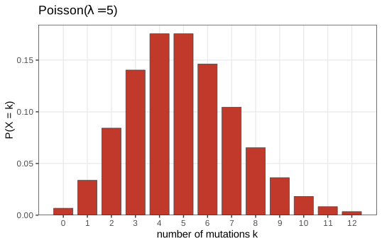
- 1.2 A count of rare independent events (mutations at \(10^4\) sites, each with probability \(5\times10^{-4}\)) is close to Poisson with mean and variance \(\lambda=5\) (Result 1.1).
- 1.3 For exchangeable categorical data the counts carry all the information (Result 1.2). Independent Bernoulli trials add up to a binomial count (Result 1.3), and when \(p\) is small the binomial is close to the Poisson: in total variation the error is at most \(np^2\) (Result 1.4). In the epitope example the right question concerns the maximum of 100 counts, whose tail probability is about 100 times the single-position one (Result 1.5); Monte Carlo estimates of such probabilities have a binomial error that we can quantify (Result 1.6, Result 1.7).
- 1.4 The multinomial distribution generalises the binomial to \(m\) categories; its margins are binomial and its covariance matrix is singular (Result 1.8). Pearson's statistic (1.1) has exact null mean \(m-1\) for every \(n\) (Result 1.9), tends to \(\chi^2_{m-1}\) (Result 1.10), and its power is approximately a noncentral chi-square probability (Result 1.11). For the book's design, 84 letters give 80% power.
Notation. \(\Pr\) is probability, \(\E\) expectation, \(\var\) variance. \(\Bern(p)\), \(\Bin(n,p)\), \(\Pois(\lambda)\) and \(\Mult(n,\mathbf{p})\) are the Bernoulli, binomial, Poisson and multinomial distributions; \(\ind\{A\}\) is the indicator of an event \(A\). For integer-valued \(X\), \(F(k)=\Pr(X\le k)\) is its distribution function and \(\Pr(X\ge k)\) its upper tail. \(\dTV(P,Q)=\sup_A|P(A)-Q(A)|\) is the total variation distance.
Prerequisites. Elementary probability (independence, expectation, variance), the binomial theorem and the exponential series. The chi-square limit in Section 1.4.1 uses the multivariate central limit theorem, stated where it is used.
1.2 A real example
Section 1.2 The book's first model concerns HIV. Suppose a mutation occurs at each nucleotide of the genome, in one replication cycle, with probability \(\mu=5\times10^{-4}\), the same at every position and independently across positions, and that the genome has \(L=10^4\) nucleotides. The number \(N\) of mutations in one cycle is then a sum of \(L\) independent indicators. The book states that \(N\) is Poisson with rate \(\lambda=L\mu=5\), so that it is "close to 5" with "variability \(\sqrt5\)", and that \(\Pr(N=3)=0.1404\). Here is where those statements come from.
Definition 1.1 (Poisson distribution)
A random variable \(X\) with values in \(\{0,1,2,\dots\}\) has the Poisson distribution with rate \(\lambda>0\), written \(X\sim\Pois(\lambda)\), if
\[ \Pr(X=k)=\frac{e^{-\lambda}\lambda^k}{k!},\qquad k=0,1,2,\dots \]Result 1.1 (moments and generating function of the Poisson distribution)
Let \(X\sim\Pois(\lambda)\). (a) The probabilities sum to one. (b) Its probability generating function is \(G(s)=\E[s^X]=e^{\lambda(s-1)}\). (c) \(\E X=\lambda\) and \(\var X=\lambda\). (d) If \(X_1\sim\Pois(\lambda_1)\) and \(X_2\sim\Pois(\lambda_2)\) are independent, \(X_1+X_2\)
Proof
(a) and (b): by the exponential series \(\sum_{k\ge0}t^k/k!=e^t\), \(\sum_k s^k e^{-\lambda}\lambda^k/k!\)
(c) The series converges for every \(s\), so it may be differentiated term by term: \(G'(s)=\E[Xs^{X-1}]\) and \(G''(s)=\E[X(X-1)s^{X-2}]\). At \(s=1\), \(\E X=G'(1)=\lambda\) and \(\E[X(X-1)]=G''(1)=\lambda^2\). Hence \(\var X\)
(d) By independence \(\E[s^{X_1+X_2}]\)
(e) The ratio is immediate from the formula. The probabilities increase while \(\lambda/k>1\) and decrease once \(\lambda/k<1\), so the largest one is at \(k=\lfloor\lambda\rfloor\); if \(\lambda\) is an integer, the ratio at \(k=\lambda\) is exactly 1. ∎
Filling the gap 1.1: why a Poisson(5), and what "variability \(\sqrt5\)" means
Let \(I_j\)
The standard deviation is not a standard error
The book calls \(\sqrt5\) "the standard error". By Result 1.1(c), \(\sqrt{\var N}=\sqrt5\approx2.24\) is the standard deviation of the count in one cycle: it describes how much \(N\) varies from one replication cycle (or one virus) to the next. A standard error is the standard deviation of an estimator. If we counted mutations in \(k\) independent cycles and estimated \(\lambda\) by the average \(\bar N\), its standard error would be \(\sqrt{\lambda/k}\), which shrinks with \(k\); the spread of \(N\) itself does not. The distinction matters in Chapter 2, where \(\lambda\) is estimated from data.
1.3 Using discrete probability models
Section 1.3 A categorical variable takes one of a finite set of values, its levels: a point mutation either occurs or not (two levels), a diploid genotype is AA, Aa or aa (three), a codon is one of 64. The book tallies the blood-group genotypes of 19 people (AA 2, AB 2, AO 7, BB 3, BO 3, OO 2) and observes that, when the order of the observations does not matter, the table of counts is all we need. Two notions make this precise.
Definition 1.2 (exchangeability)
A random sequence \((X_1,\dots,X_n)\) is exchangeable if for every permutation \(\sigma\) of \(\{1,\dots,n\}\) the permuted sequence \((X_{\sigma(1)},\dots,X_{\sigma(n)})\) has the same joint distribution as \((X_1,\dots,X_n)\). Independent and identically distributed (iid) sequences are exchangeable; the converse is false (draws without replacement from an urn are exchangeable but dependent).
Result 1.2 (for exchangeable categorical data the counts are sufficient)
Let \((X_1,\dots,X_n)\) be exchangeable with values in levels \(\{1,\dots,m\}\), and let \(\mathbf{C}=(C_1,\dots,C_m)\), \(C_i=\#\{t:X_t=i\}\), be the vector of counts. Given \(\mathbf{C}=\mathbf{c}\), every sequence with these counts is equally likely, with conditional probability \(c_1!\cdots c_m!/n!\). In particular, for iid draws with \(\Pr(X_t=i)=p_i\), the likelihood \(\prod_ip_i^{c_i}\) depends on the data only through \(\mathbf{c}\): the counts are a sufficient statistic for \(\mathbf{p}\).
Proof
Fix a sequence \(\mathbf{x}\) with counts \(\mathbf{c}\). Every other sequence with the same counts is a permutation of \(\mathbf{x}\), so by exchangeability all of them have the same probability \(\Pr(\mathbf{X}=\mathbf{x})\). There are \(n!/(c_1!\cdots c_m!)\) of them (Filling the gap 1.7). The event \(\{\mathbf{C}=\mathbf{c}\}\) is their disjoint union, so \(\Pr(\mathbf{X}\)
Check. For six iid \(\Bern(0.3)\) trials, the 64 sequences grouped by their number of successes have equal conditional probabilities within every group (to \(10^{-15}\)).
Question 1.1. A factor can be given levels that do not occur in the data with the levels argument, e.g. factor(genotype, levels = c("AA", "AB", "AO", "BB", "BO", "OO", "A?")); table() then reports a zero count for the unseen level. This matters for counts: a level with zero count is information (it was possible and did not occur), which a table that silently drops it would lose.
1.3.1 Bernoulli trials
Section 1.3.1 The simplest random experiment has two outcomes, coded 1 ("success") and 0. A ball falls into the right-hand box of Figure 1.2 (a drawing of two boxes of unequal size) with probability \(2/3\) and into the left-hand box otherwise.
Definition 1.3 (Bernoulli and binomial distributions)
\(X\sim\Bern(p)\) if \(\Pr(X=1)=p\) and \(\Pr(X=0)=1-p\), \(0\le p\le1\). If \(X_1,\dots,X_n\) are independent \(\Bern(p)\), their sum \(K=\sum_tX_t\), the number of successes, has the binomial distribution \(\Bin(n,p)\). The book writes \(B(n,p)\).
Algorithm 1.1 (simulating a discrete random variable from a uniform one: inversion)
Input: probabilities \(p_1,\dots,p_m\) of levels \(1,\dots,m\) (summing to 1). Put \(c_0=0\) and \(c_j=p_1+\dots+p_j\).
- Draw \(U\) uniform on \((0,1)\) (in R,
runif(1)). - Return \(X=\min\{j:U\le c_j\}\).
Then \(\Pr(X\)c("A","C","G","T")[findInterval(runif(n), c(0, 1, 4, 7, 8)/8)]. A chi-square goodness-of-fit test on \(10^5\) such draws accepts these probabilities.
Question 1.2. Repeated calls to rbinom(15, prob = 0.5, size = 1) give different answers because each call advances the state of R's pseudo-random number generator; the sequence is deterministic given the starting state, which set.seed() fixes. Every figure function in the course code calls set.seed() so that it reproduces exactly.
1.3.2 Binomial success counts
Section 1.3.2 If the trials are exchangeable, only the number of successes matters (Result 1.2): SSSSSFSSSSFFFSF becomes \(k=10\) out of \(n=15\). The book states the probability of \(k\) successes.
Filling the gap 1.2: the binomial probability by counting
Claim: if \(K\sim\Bin(n,p)\) then, for \(k=0,1,\dots,n\),
\[ \Pr(K=k)=\binom nk p^k(1-p)^{n-k},\qquad \binom nk=\frac{n!}{k!\,(n-k)!}=\frac{n(n-1)\cdots(n-k+1)}{k(k-1)\cdots1}. \]Derivation
A particular sequence of outcomes \((x_1,\dots,x_n)\in\{0,1\}^n\) with \(k\) ones has probability \(\prod_tp^{x_t}(1-p)^{1-x_t}\)
Result 1.3 (mean, variance and mode of the binomial)
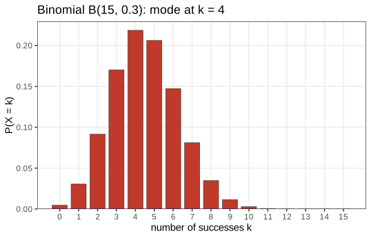
If \(K\sim\Bin(n,p)\) with \(0<p<1\): \(\E K=np\), \(\var K=np(1-p)\), and the mode is \(\lfloor(n+1)p\rfloor\) (when \((n+1)p\) is an integer, \((n+1)p-1\) is a second mode).
Proof
Write \(K=\sum_tX_t\) with independent \(X_t\sim\Bern(p)\). Each has \(\E X_t=p\) and, since \(X_t^2=X_t\), \(\var X_t=p-p^2\). Expectations add, and so do variances of independent variables: \(\E K=np\), \(\var K=np(1-p)\).
For the mode, the ratio of successive probabilities is
\[ r_k=\frac{\Pr(K=k)}{\Pr(K=k-1)}=\frac{(n-k+1)\,p}{k\,(1-p)},\qquad k=1,\dots,n, \]and \(r_k\)
Check. The mode formula holds on a grid of 360 pairs \((n,p)\).
Question 1.3. For \(\Bin(15,0.3)\), \((n+1)p=4.8\), so the most common outcome is 4, with probability 0.2186 (Figure 1.3). Ten repetitions of rbinom(1, prob = 0.3, size = 15) are too few to see this reliably: 4 is the strictly most frequent value among ten draws only about 23% of the time (by simulation).
Question 1.4. For \(k=3\), \(p=2/3\), \(n=4\): \(\binom43(2/3)^3(1/3)\)dbinom(3, 4, 2/3)).
1.3.3 Poisson distributions
Section 1.3.3 (Figure 1.4 is a portrait of Siméon Denis Poisson.) The book states that when \(n\) is large and \(p\) small, \(\Bin(n,p)\) "can be faithfully approximated" by \(\Pois(np)\), and checks it on the HIV numbers. The approximation has two classical forms: a limit theorem, and an explicit error bound that says how faithful "faithfully" is.
Result 1.4 (the Poisson limit and Le Cam's inequality)
(a) Limit. If \(n\to\infty\) and \(p_n\to0\) with \(np_n\to\lambda\in(0,\infty)\), then for every fixed \(k\), \(\Pr(\Bin(n,p_n)\)
(b) Error bound. Let \(X_1,\dots,X_n\) be independent with \(X_i\sim\Bern(p_i)\), \(S=\sum_iX_i\) and \(\lambda=\sum_ip_i\). Then
\[ \dTV\big(\mathcal{L}(S),\Pois(\lambda)\big)\le\sum_{i=1}^np_i^2, \qquad\text{in particular}\qquad \dTV\big(\Bin(n,p),\Pois(np)\big)\le np^2. \](c) A sharper bound (Barbour and Hall's refinement, stated without proof) is \(\dTV\)
Here \(\dTV(P,Q)\)
Filling the gap 1.3: proof of the Poisson limit, Result 1.4(a)
Proof
Fix \(k\) and write \(\lambda_n=np_n\). Then
\[ \Pr(\Bin(n,p_n)=k)=\frac{n(n-1)\cdots(n-k+1)}{n^k}\cdot\frac{\lambda_n^k}{k!}\cdot\Big(1-\frac{\lambda_n}{n}\Big)^{n}\cdot\Big(1-\frac{\lambda_n}{n}\Big)^{-k}. \]The first factor is a product of \(k\) terms \((1-j/n)\to1\); the second tends to \(\lambda^k/k!\); the last tends to 1 because \(\lambda_n/n=p_n\to0\) and \(k\) is fixed. For the third, \(n\log(1-\lambda_n/n)\)
The limit is pointwise; because the limiting probabilities sum to one, pointwise convergence of probability mass functions on the integers implies convergence in total variation (Scheffé's lemma), but it gives no rate. Part (b) does.
Filling the gap 1.4: Le Cam's inequality by coupling, Result 1.4(b)
Proof
Step 1 (coupling inequality). If \(S\) and \(T\) are any two random variables defined on the same probability space, then for every event \(A\), \(\Pr(S\in A)-\Pr(T\in A)\)
Step 2 (one trial). Let \(U\) be uniform on \((0,1)\) and \(q\in(0,1)\). Put \(X=\ind\{U>1-q\}\sim\Bern(q)\) and let \(Y=F_q^{-1}(U)\) be the Poisson(\(q\)) variable obtained by inversion (Algorithm 1.1): \(Y=0\) if \(U\le e^{-q}\), \(Y=1\) if \(e^{-q}<U\le e^{-q}(1+q)\), and so on. Since \(1-q\le e^{-q}\), we have \(X=Y=0\) for \(U\le1-q\) and \(X=Y=1\) for \(e^{-q}<U\le e^{-q}(1+q)\). They differ only when \(1-q<U\le e^{-q}\) (then \(X=1,Y=0\)) or when \(Y\ge2\). Therefore
\[ \Pr(X\ne Y)=\big(e^{-q}-(1-q)\big)+\big(1-e^{-q}-qe^{-q}\big)=q\,(1-e^{-q})\le q^2, \]using \(1-e^{-q}\le q\).
Step 3 (sum). Build independent pairs \((X_i,Y_i)\) as in Step 2 with \(q=p_i\), from independent uniforms \(U_i\). Then \(S=\sum X_i\) has the required distribution and \(T=\sum Y_i\sim\Pois(\lambda)\) by Result 1.1(d). If \(S\ne T\) then \(X_i\ne Y_i\) for some \(i\), so by the union bound \(\Pr(S\)
Checks. The coupling probability \(q(1-e^{-q})\) is confirmed by simulation, and both bounds of Result 1.4 hold for all 36 pairs of a grid \(n\in\{5,\dots,10^4\}\), \(p\in\{10^{-4},\dots,0.3\}\), with the exact distance computed by summation.
The bound tells us where the approximation is good and where it is not:
| Example | \(n\), \(p\) | exact \(\dTV\) | Le Cam \(np^2\) | \((1-e^{-np})p\) |
|---|---|---|---|---|
| HIV mutations (Figure 1.1) | \(10^4\), \(5\times10^{-4}\) | 0.000122 | 0.0025 | 0.000497 |
| ELISA background, 50 patients (Section 1.3.4) | 50, 0.01 | 0.00229 | 0.005 | 0.00393 |
| \(\Bin(15,0.3)\) (Figure 1.3) | 15, 0.3 | 0.0846 | 1.35 | 0.297 |
For \(\Bin(15,0.3)\) the Poisson(4.5) is a poor model: its variance 4.5 exceeds the binomial variance \(np(1-p)=3.15\), and the two distributions differ by 8.5 percentage points on some event. The rule of thumb is therefore not "\(n\) large" but "\(p\) small": the error is controlled by \(p\) times a factor at most 1.
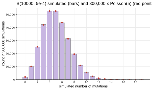
Question 1.5. For \(n=10^4\), \(p=5\times10^{-4}\) the probabilities of 0 to 12 mutations under \(\Bin(n,p)\) and \(\Pois(5)\) agree to within \(4.4\times10^{-5}\) (dbinom(0:12, 1e4, 5e-4) - dpois(0:12, 5)), well inside the bound \(1.22\times10^{-4}\) on every event.
The book then simulates the mutation process: 300,000 draws of the number of mutations, each a \(\Bin(10^4,5\times10^{-4})\) count (Figure 1.5).
1.3.4 A generative model for epitope detection
Section 1.3.4 An epitope is the part of an antigen recognised by an antibody or a T cell receptor (Figure 1.6 is a diagram of an antibody). An ELISA (enzyme-linked immunosorbent assay) array tests for epitopes at many positions of a protein. The data are 0/1 calls: 1 means the assay declares a hit.
ELISA error model with known parameters
The book's assumptions, written as a probability model: let \(Y_{ij}\in\{0,1\}\) be the call for patient \(i=1,\dots,50\) at position \(j=1,\dots,100\). If the protein carries no epitope, the \(Y_{ij}\) are independent with \(\Pr(Y_{ij}=1)=f=0.01\), the false positive rate. The data analysed are the column totals
\[ X_j=\sum_{i=1}^{50}Y_{ij}\sim\Bin(50,0.01),\qquad j=1,\dots,100,\ \text{independent}. \]The book models each \(X_j\) as \(\Pois(0.5)\) (the Task in this subsection asks to verify this by simulation). By Result 1.4 the two models differ by at most \(50\times0.01^2=0.005\) on any event, and in fact by 0.0023. The Poisson model is used below, as in the book. One caution: a total variation bound controls absolute errors, and the tail probabilities below are of order \(10^{-6}\). Under the exact binomial model \(\Pr(X_j\ge7)=6.85\times10^{-7}\) instead of the Poisson \(1.00\times10^{-6}\), so the Poisson answer is conservative here by about 30% in relative terms; none of the conclusions change.
One patient's data and the results of the 50 assays
One patient's 100 calls contain a single 1 (at position 22 in the book's display). Summed over 50 patients, typical background data look like Figure 1.7; the observed data, the vector e100 of the book's data folder, are in Figure 1.8. Their mean is 0.55; the counts are 0 (58 positions), 1 (34), 2 (7) and, at position 42, 7.
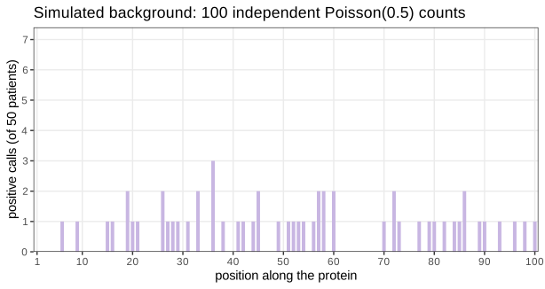
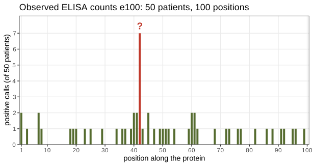
e100: positive calls among 50 patients at each of 100 positions. The spike of 7 at position 42 (red) is the question of this section. Reproduces Holmes and Huber (2019), Figure 1.8. Download: PDF · SVGFor a single position, the probability of a count of at least 7 under \(\Pois(0.5)\) is
\[ \epsilon=\Pr(X\ge7)=\sum_{k\ge7}\frac{e^{-0.5}0.5^k}{k!}=1.00238\times10^{-6}. \]The book computes it as ppois(6, 0.5, lower.tail = FALSE) and notes that this is more accurate than 1 - ppois(6, 0.5). The reason is cancellation: \(1-F(6)\) subtracts two numbers that agree in their first six digits, and the absolute rounding error of \(F(6)\) (about \(10^{-16}\)) becomes a relative error of about \(10^{-10}\) in \(\epsilon\); summing the small terms of the tail directly keeps full relative precision. Here both agree to \(10^{-17}\), but for tails near \(10^{-16}\) the subtraction returns 0.
Extreme value analysis for the Poisson distribution
Question 1.6 asks for the flaw in reporting \(\epsilon\). The value 7 was not observed at a position chosen in advance: it was found by scanning all 100 positions and taking the largest. The relevant statistic is the maximum \(M=\max_jX_j\), and the relevant probability is \(\Pr(M\ge7)\) under the null model.
Result 1.5 (the maximum of independent counts)
Let \(X_1,\dots,X_n\) be independent with common distribution function \(F\), let \(M=\max_jX_j\), and for an integer threshold \(m\) let \(\epsilon=\Pr(X_1\ge m)\). Then
\[ \Pr(M\le k)=F(k)^n,\qquad \Pr(M\ge m)=1-(1-\epsilon)^n, \]and
\[ n\epsilon-\binom n2\epsilon^2\;\le\;\Pr(M\ge m)\;\le\;n\epsilon,\qquad 0\le\Pr(M\ge m)-\big(1-e^{-n\epsilon}\big)\le n\epsilon^2\quad(\epsilon\le\tfrac12). \]Filling the gap 1.5: the distribution of the maximum and its approximations
Proof of Result 1.5
Exact formula. The maximum is at most \(k\) exactly when every \(X_j\) is at most \(k\): \(\{M\le k\}=\bigcap_j\{X_j\le k\}\). By independence \(\Pr(M\)
Union and Bonferroni bounds. Let \(A_j=\{X_j\ge m\}\) and \(Z=\sum_j\ind_{A_j}\), the number of positions at or above the threshold, so \(\{M\ge m\}=\{Z\ge1\}\). For every integer \(z\ge0\), \(z-\binom z2\le\ind\{z\ge1\}\le z\): both sides are 0 at \(z=0\); for \(z\ge1\) the right inequality is clear and the left one reads \(z(3-z)/2\le1\), true for every integer. Take expectations: \(\E Z=n\epsilon\) and \(\E\binom Z2\)
Exponential approximation. Since \(1-\epsilon\le e^{-\epsilon}\), \((1-\epsilon)^n\le e^{-n\epsilon}\), so the difference is nonnegative. For \(0\le\epsilon\le\frac12\), \(\log(1-\epsilon)\)
With \(n=100\) and \(\epsilon=1.00238\times10^{-6}\): the exact value is \(\Pr(M\ge7)=1.0023299\times10^{-4}\); the book's approximation \(1-e^{-n\epsilon}\) gives \(1.0023294\times10^{-4}\) (difference \(5\times10^{-11}\), below the bound \(n\epsilon^2=10^{-10}\)); the union bound gives \(1.00238\times10^{-4}\). All three are 100 times \(\epsilon\) to three digits. The book derives the same thing through the binomial expansion of \((1-\epsilon)^{100}\) and through \(\log(1-\epsilon)\approx-\epsilon\); the inequalities above make those "\(\simeq\)" steps exact.
Erratum (order statistics). The book's derivation writes \(\Pr(x_{(100)}\)
Multiplicity. The step from \(\epsilon\) to \(1-(1-\epsilon)^n\) is the simplest instance of a multiple-testing correction: if each of \(n\) independent positions has p-value \(p_j\) and we report the smallest, \(1-(1-p_{\min})^n\) is the adjusted p-value (the Šidák form), and \(np_{\min}\) is the Bonferroni form, its upper bound by Result 1.5. Chapter 6 of the book develops this.
Computing probabilities by simulation
The book's Monte Carlo experiment draws 100,000 data sets of 100 \(\Pois(0.5)\) counts and records how often the maximum reaches 7: 16 times, an estimate of \(1.6\times10^{-4}\), which "more or less agrees" with \(10^{-4}\). It also notes that the estimate has a granularity of \(10^{-5}\). How large is the Monte Carlo error, and how should a Monte Carlo p-value be reported?
Result 1.6 (Monte Carlo estimate of a probability, with its error)
Let \(T_1,\dots,T_B\) be independent simulations of a statistic \(T\) and \(p=\Pr(T\in A)\). The number of hits \(K=\sum_b\ind\{T_b\in A\}\) is \(\Bin(B,p)\), and the estimate \(\hat p=K/B\) satisfies:
- \(\E\hat p=p\) and \(\operatorname{se}(\hat p)\)
\({}=\sqrt{p(1-p)/B}\); the relative error is \(\operatorname{se}/p\) \({}=\sqrt{(1-p)/(Bp)}\) \({}\approx1/\sqrt{\E K}\). - \(\hat p\) only takes the values \(0,1/B,2/B,\dots\) (the book's granularity), but the error is set by \(\operatorname{se}\), which for small \(p\) is much larger than \(1/B\).
- (Clopper–Pearson) With \(\Beta(a,b)\) quantiles \(q_\gamma(a,b)\), the interval \[ \big[q_{\alpha/2}(K,B-K+1),\ q_{1-\alpha/2}(K+1,B-K)\big] \] (lower end 0 if \(K=0\), upper end 1 if \(K=B\)) covers \(p\) with probability at least \(1-\alpha\), for every \(p\) and \(B\).
- If \(K=0\), the one-sided upper confidence bound is \(1-\alpha^{1/B}\)
\({}\approx-\log(\alpha)/B\), which is about \(3/B\) for \(\alpha=0.05\).
Filling the gap 1.6: proof of Result 1.6 and what it says about the book's simulation
Proof
1 and 2 are Result 1.3 divided by \(B\) (and by \(B^2\) for the variance).
3. A binomial tail is a beta probability. Let \(U_1,\dots,U_B\) be iid uniform on \((0,1)\), with order statistics \(U_{(1)}\le\dots\le U_{(B)}\). The number of \(U_b\le p\) is \(\Bin(B,p)\), and it is at least \(k\) exactly when \(U_{(k)}\le p\). The density of \(U_{(k)}\) is \(\frac{B!}{(k-1)!(B-k)!}u^{k-1}(1-u)^{B-k}\) (one of the \(B\) points sits at \(u\), \(k-1\) are below, \(B-k\) above), i.e. \(U_{(k)}\sim\Beta(k,B-k+1)\). Hence
\[ \Pr(\Bin(B,p)\ge k)=\Pr\big(\Beta(k,B-k+1)\le p\big). \]Coverage. Let \(L(k)=q_{\alpha/2}(k,B-k+1)\) for \(k\ge1\) and \(L(0)=0\). By the identity, \(L(k)\) is the value of \(p\) at which \(\Pr_p(K\ge k)=\alpha/2\), and \(\Pr_p(K\ge k)\) is continuous and increasing in \(p\); hence \(L(k)>p\iff\Pr_p(K\ge k)<\alpha/2\). Fix the true \(p\) and let \(k^*\) be the smallest \(k\) with \(\Pr_p(K\ge k)<\alpha/2\). Because \(\Pr_p(K\ge k)\) decreases in \(k\), \(\{L(K)>p\}=\{K\ge k^*\}\), an event of probability \(\Pr_p(K\ge k^*)<\alpha/2\). The upper end is handled symmetrically with \(\Pr(\Bin(B,p)\)
4. With \(K=0\) the one-sided bound solves \(\Pr_p(K=0)=(1-p)^B=\alpha\), so \(p=1-\alpha^{1/B}\)
The book's run. With \(p\approx10^{-4}\) and \(B=10^5\), \(\E K=10\): the standard error is \(3.2\times10^{-5}\), a relative error of about 32%, far coarser than the granularity \(10^{-5}\). The observed \(K=16\) gives the 95% interval \([0.91,\,2.60]\times10^{-4}\), which contains the exact value \(1.0023\times10^{-4}\); the "more or less agreement" is exactly what the binomial error predicts (\(K=16\) is 1.9 standard deviations above 10). To estimate \(10^{-4}\) to 10% one needs \(\E K\approx100\), i.e. \(B\approx10^6\) simulations.
Result 1.7 (a Monte Carlo p-value is valid)
Let \(t_0\) be the observed statistic and \(T_1,\dots,T_B\) independent simulations from the null model. If, under the null, \(T_0,T_1,\dots,T_B\) are exchangeable (e.g. iid), then
\[ \hat p_{\mathrm{MC}}=\frac{1+\#\{b:T_b\ge T_0\}}{B+1} \]satisfies \(\Pr(\hat p_{\mathrm{MC}}\)
Proof
Suppose first there are no ties. Let \(R\) be the rank of \(T_0\) from the top among the \(B+1\) values (\(R=1\) for the largest). By exchangeability every position is equally likely for \(T_0\), so \(R\) is uniform on \(\{1,\dots,B+1\}\). Since \(\hat p_{\mathrm{MC}}=R/(B+1)\), \(\Pr(\hat p_{\mathrm{MC}}\)
Check. With \(B=19\) and a continuous statistic, \(\Pr(\hat p_{\mathrm{MC}}\)
The naive estimate \(K/B\) can be 0, which is not a valid p-value: it would claim that the observed data are impossible under the null. The book's estimate 0.00016 should be reported as \((1+16)/(100{,}001)\)
Algorithm 1.2 (Monte Carlo test for the epitope spike)
- Compute the observed statistic \(t_0=\max_jx_j\) (here 7).
- For \(b=1,\dots,B\): simulate \(x^{(b)}_1,\dots,x^{(b)}_{100}\) independently from \(\Pois(\lambda)\) and record \(t_b=\max_jx^{(b)}_j\).
- Report \(\hat p_{\mathrm{MC}}\)
\({}=(1+\#\{b:t_b\ge t_0\})/(B+1)\), \(B\), and a Clopper–Pearson interval for the hit rate (Result 1.6).
Only the ability to simulate from the null model is required: no formula for the distribution of the statistic. The procedure works unchanged for statistics with no closed-form distribution (the second-largest count, the longest run of positive positions, a smoothed score), which is the book's point. In R: tb <- replicate(B, max(rpois(100, lambda))); (1 + sum(tb >= 7)) / (B + 1).
Known parameters. All of this is probability: \(\lambda=0.5\) is known from the false positive rate. If \(\lambda\) is estimated from the same data (Exercise 1.3 plugs in the mean 0.55, which includes the spike), the null distribution of the statistic changes, because the estimate itself varies from data set to data set; Chapter 2 of the book turns to this statistical modelling. (The data file is itself a simulation: the book's source generates 100 \(\Pois(0.5)\) counts and sets position 42 to 7.)
1.4 Multinomial distributions: the case of DNA
Section 1.4 With more than two outcomes, for instance the four nucleotides, a single draw lands in one of \(m\) boxes of probabilities \(p_1,\dots,p_m\) (Figure 1.9 is a drawing of four boxes of different sizes), and \(n\) independent draws are summarised by the counts in the boxes.
Definition 1.4 (multinomial distribution)
Let \(C_1,\dots,C_n\) be iid with \(\Pr(C_t=i)=p_i\), \(i=1,\dots,m\), \(\sum_ip_i=1\), and \(X_i=\#\{t:C_t=i\}\). The vector \(\mathbf{X}=(X_1,\dots,X_m)\) has the multinomial distribution \(\Mult(n,\mathbf{p})\). Its support is the set of count vectors with \(x_i\ge0\) and \(\sum_ix_i=n\); there are \(\binom{n+m-1}{m-1}\) of them (165 for \(n=8\), \(m=4\); 1771 for \(n=20\)).
Filling the gap 1.7: the multinomial probability and the multinomial coefficient
Claim (the book's formula):
\[ \Pr(\mathbf{X}=\mathbf{x})=\frac{n!}{x_1!\,x_2!\cdots x_m!}\,p_1^{x_1}p_2^{x_2}\cdots p_m^{x_m},\qquad \textstyle\sum_ix_i=n. \]Derivation
Each sequence \((c_1,\dots,c_n)\) with counts \(\mathbf{x}\) has probability \(\prod_tp_{c_t}=\prod_ip_i^{x_i}\) by independence. The number of such sequences: choose the \(x_1\) positions of level 1 in \(\binom n{x_1}\) ways, then the \(x_2\) positions of level 2 among the remaining \(n-x_1\) in \(\binom{n-x_1}{x_2}\) ways, and so on. The product telescopes:
\[ \binom n{x_1}\binom{n-x_1}{x_2}\cdots\binom{x_m}{x_m}=\frac{n!}{x_1!\,(n-x_1)!}\cdot\frac{(n-x_1)!}{x_2!\,(n-x_1-x_2)!}\cdots=\frac{n!}{x_1!\cdots x_m!}. \]The probabilities sum to one by the multinomial theorem \((p_1+\dots+p_m)^n\)
Question 1.7. Four equally likely boxes, counts \((4,2,0,0)\), \(n=6\): \(\frac{6!}{4!\,2!\,0!\,0!}\cdot4^{-6}\)dmultinom(c(4, 2, 0, 0), prob = rep(1/4, 4)) returns.
Result 1.8 (margins, merging, conditioning and moments of the multinomial)
Let \(\mathbf{X}\sim\Mult(n,\mathbf{p})\).
- Margins. \(X_i\sim\Bin(n,p_i)\).
- Merging. If the levels are grouped into disjoint sets \(G_1,\dots,G_r\), the group totals are \(\Mult\big(n,(\sum_{i\in G_1}p_i,\dots,\sum_{i\in G_r}p_i)\big)\). For example purines A+G against pyrimidines C+T is binomial.
- Conditioning. Given \(X_m=x_m\), the other counts are multinomial: \[ (X_1,\dots,X_{m-1})\sim\Mult\Big(n-x_m,\ \frac{(p_1,\dots,p_{m-1})}{1-p_m}\Big). \]
- Moments. \(\E\mathbf{X}=n\mathbf{p}\), \(\var X_i=np_i(1-p_i)\), \(\cov(X_i,X_j)=-np_ip_j\) for \(i\ne j\); that is, \(\cov(\mathbf{X})\)
\({}=n\big(\diag(\mathbf{p})-\mathbf{p}\mathbf{p}^\T\big)\). This matrix is singular: \(\mathbf{1}\) is in its null space, because \(\sum_iX_i=n\) is not random. - Poisson representation. If \(Y_1,\dots,Y_m\) are independent \(\Pois(\lambda p_i)\), then given \(\sum_iY_i=n\), \((Y_1,\dots,Y_m)\)
\({}\sim\Mult(n,\mathbf{p})\).
Proof
1 and 2: in the construction of Definition 1.4, the indicator that draw \(t\) lands in group \(G_s\) has probability \(\sum_{i\in G_s}p_i\), and the group labels of the draws are iid; so the group totals are multinomial by definition. Part 1 is the grouping \(\{i\}\) against the rest.
3: for counts \(x_1,\dots,x_{m-1}\) summing to \(n-x_m\), divide the multinomial probability by the binomial probability of \(X_m=x_m\):
\[ \frac{\frac{n!}{x_1!\cdots x_m!}\prod_{i\le m}p_i^{x_i}}{\frac{n!}{x_m!\,(n-x_m)!}p_m^{x_m}(1-p_m)^{n-x_m}}=\frac{(n-x_m)!}{x_1!\cdots x_{m-1}!}\prod_{i<m}\Big(\frac{p_i}{1-p_m}\Big)^{x_i}, \]using \(\sum_{i<m}x_i=n-x_m\).
4: write \(\mathbf{X}=\sum_t\mathbf{e}_{C_t}\), a sum of iid one-hot vectors (\(\mathbf{e}_i\) is the \(i\)th unit vector). One draw has \(\E\mathbf{e}_{C}=\mathbf{p}\) and \(\E[\mathbf{e}_C\mathbf{e}_C^\T]\)
5: \(\sum_iY_i\sim\Pois(\lambda)\) by Result 1.1(d), so for \(\sum x_i=n\), \(\Pr(\mathbf{Y}\)
Checks. Parts 1–4 are confirmed by exact enumeration of all 165 count vectors with \(n=8\), \(\mathbf{p}=(3,2,2,1)/8\).
Question 1.8. t() is the matrix transpose. rmultinom returns one column per draw, so t() turns the \(4\times1\) result into a row for display.
Question 1.9. rmultinom(n = 8, prob = pvec, size = 1) draws eight single letters: a \(4\times8\) matrix of one-hot columns, i.e. the sequence. rmultinom(n = 1, prob = pvec, size = 8) draws one count vector for eight letters. The row sums of the first have the same distribution as the second (that is Definition 1.4), exactly as eight Bernoulli trials summed give one binomial count (Sections 1.3.1 and 1.3.2); the first keeps the order, which by Result 1.2 carries no further information about \(\mathbf{p}\).
1.4.1 Simulating for power
Section 1.4.1 How long must a DNA sequence be before we can tell a fair process, with all four nucleotides equally likely, from a specific alternative? The book answers by simulation; here are the definitions it uses, then the exact answers.
Definition 1.5 (test, null distribution, size, power, p-value)
A test of a null hypothesis \(H_0\) is a statistic \(T\) and a rule "reject \(H_0\) if \(T>c\)". The distribution of \(T\) when \(H_0\) holds is its null distribution. The size of the test is \(\Pr_{H_0}(T>c)\); a test has level \(\alpha\) if its size is at most \(\alpha\). Its power against an alternative \(H_A\) is \(\Pr_{H_A}(T>c)\), the true positive rate. The p-value of an observed value \(t_0\) is \(\Pr_{H_0}(T\ge t_0)\), the null probability of a result at least as extreme as the one observed.
The book's null is \(H_0:\mathbf{p}\)
Creating a test
For observed counts \(\mathbf{x}\) and expected counts \(E_i=np_{0i}\) under the null, the book's statistic is Pearson's
\[ S=\sum_{i=1}^m\frac{(x_i-E_i)^2}{E_i}. \tag{1.1} \]The book simulates 1000 sequences of length 20 under \(H_0\), finds that the simulated values have mean 3.126, and takes their 95% quantile, 7.6, as the critical value. The exact mean of \(S\) is known.
Result 1.9 (exact mean and variance of Pearson's statistic under the null)
If \(\mathbf{X}\sim\Mult(n,\mathbf{p})\) with all \(p_i>0\) and \(S=\sum_i(X_i-np_i)^2/(np_i)\), then for every \(n\ge1\)
\[ \E S=m-1,\qquad \var S=2(m-1)+\frac1n\Big(\sum_{i=1}^m\frac1{p_i}-m^2-2m+2\Big). \]For equal probabilities \(\sum_i1/p_i=m^2\) and \(\var S=2(m-1)(1-1/n)\): with \(m=4\), \(n=20\), \(\E S=3\) and \(\var S=5.7\).
Filling the gap 1.8: proof of Result 1.9 by factorial moments
Derivation
Mean. \(\E(X_i-np_i)^2\)
A simpler form. Expanding the square and using \(\sum_iX_i=n\), \(\sum_ip_i=1\): \(S\)
Factorial moments. Write \(a^{(r)}=a(a-1)\cdots(a-r+1)\). For the multinomial, \(\E X_i^{(r)}=n^{(r)}p_i^r\) and, for \(i\ne j\), \(\E[X_i^{(r)}X_j^{(s)}]\)
Second moment of \(Q\). \(\E Q\)
Summing over \(i\) and over ordered pairs \(i\ne j\), with \(\sum_{i\ne j}p_ip_j=1-\sum_ip_i^2\), \(\sum_{i\ne j}(p_i+p_j)=2(m-1)\) and \(m(m-1)\) ordered pairs:
\[ \E Q^2=n^{(4)}+n^{(3)}(2m+4)+n^{(2)}(m^2+6m)+n\sum_i\frac1{p_i}. \]Variance. Subtract \((\E Q)^2\)
so
\[ \begin{aligned}\var Q&=n(n-1)(m^2+2m-2)+n\textstyle\sum_i1/p_i-n^2m^2\\ &=2(m-1)n^2+n\big(\textstyle\sum_i1/p_i-m^2-2m+2\big).\end{aligned} \]Divide by \(n^2\). ∎
Checks. Exact enumeration of all 1771 count vectors gives \(\E S=3\) and \(\var S=5.7\) at \(n=20\) for the uniform null, and the general formula for the null \((3,2,2,1)/8\).
The book's simulation. With 1000 simulated values the standard error of their mean is \(\sqrt{5.7/1000}=0.075\), so the book's 3.126 is 1.7 standard errors above the exact 3: consistent. The standard deviation of \(S\) is \(\sqrt{5.7}=2.39\), smaller than the \(\sqrt6=2.45\) of the limiting \(\chi^2_3\).
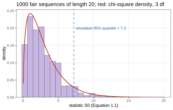
The null distribution is discrete. For the uniform null, \(S=\frac mn\sum_ix_i^2-n\); since \(x^2\equiv x\pmod2\), \(\sum_ix_i^2\) has the parity of \(n\), so with \(m=4\), \(n=20\), \(S=\frac15\sum x_i^2-20\) takes values in \(\{0,0.4,0.8,\dots\}\). There is therefore no critical value with size exactly 0.05, and the simulated quantile depends on the run (7.6 in the book's, 7.2 in ours). The exact distribution can be computed instead of simulated:
Algorithm 1.3 (exact null distribution and exact level-\(\alpha\) test by enumeration)
- List every count vector \(\mathbf{x}\) with \(\sum_ix_i=n\) (\(\binom{n+m-1}{m-1}\) of them) and compute \(S(\mathbf{x})\), its null probability \(f_0(\mathbf{x})\) and its alternative probability \(f_A(\mathbf{x})\) from Filling the gap 1.7.
- Sort the distinct values of \(S\) and accumulate \(f_0\): this is the exact null distribution function.
- Take the critical value \(c\) as the smallest value of \(S\) with \(\Pr_0(S\le c)\ge1-\alpha\), and reject when \(S>c\). Then the size \(\Pr_0(S>c)\le\alpha\), and the power is \(\sum_{\mathbf{x}:S(\mathbf{x})>c}f_A(\mathbf{x})\).
For \(n=20\) (1771 vectors) this gives \(c=7.6\), the same as the book's simulated quantile, with exact size \(\Pr_0(S>7.6)=0.0415\); the value 7.6 itself has null probability 0.0187, so \(\Pr_0(S\ge7.6)=0.0602\). (The demonstration computes this exactly in the browser.)
Determining the test's power
The book simulates 1000 sequences under \(\mathbf{p}_A\), finds that 199 have \(S>7.6\), and reports a power of 0.199. The exact power of the same rule, by Algorithm 1.3, is 0.1998. The book's first alternative sequence, \((10,3,5,2)\), has \(S=7.6\) exactly; it is not rejected only because the rule is a strict inequality, a tie that the discreteness makes common.
Algorithm 1.4 (power by simulation, the book's procedure)
- Simulate \(B\) count vectors under \(H_0\), compute \(S\) for each, and let \(c\) be their 95% quantile (or use the exact \(c\) of Algorithm 1.3).
- Simulate \(B\) count vectors under \(H_A\) and compute \(S\) for each.
- The power estimate is the fraction of alternative values with \(S>c\); its standard error is \(\sqrt{\hat\beta(1-\hat\beta)/B}\) (Result 1.6), 0.013 for \(B=1000\) and \(\hat\beta=0.2\).
Task: the sequence length for 80% power. The exact power (Algorithm 1.3, with the exact level-0.05 critical value at each \(n\)) first reaches 0.8 at \(n=84\) (power 0.802), and stays above 0.8 for every \(n\) from 84 to 110. It is not monotone in \(n\): because of the discreteness, the power at \(n=68\) (0.685) is lower than at \(n=67\) (0.690), and similar dips occur at 93 and 106. The noncentral chi-square approximation of Result 1.11 gives \(n=88\), and simulation with \(B=10{,}000\) at \(n=84\) agrees with the exact answer to within its standard error.
Classical statistics for classical data
The book closes the section by stating that \(S\) "has a well-known distribution called the chi-square distribution (with 3 degrees of freedom)". That is true only in the limit \(n\to\infty\): for \(n=20\) the distribution of \(S\) is the discrete one above, with variance 5.7 instead of 6, and the chi-square cutoff 7.815 has exact size 0.0415 instead of 0.05. Here is the limit theorem, and the companion result for power. (Figure 1.11 of the book is a schematic of a probability model \(F_\theta\) generating data \(x\); it is not reproduced.)
Result 1.10 (Pearson's statistic is asymptotically \(\chi^2_{m-1}\))
If \(\mathbf{X}\sim\Mult(n,\mathbf{p})\) with all \(p_i>0\), then as \(n\to\infty\), \(S=\sum_i(X_i-np_i)^2/(np_i)\) converges in distribution to \(\chi^2_{m-1}\); in particular \(\Pr(S>c)\to\Pr(\chi^2_{m-1}>c)\) for every \(c\).
Filling the gap 1.9: proof of the chi-square limit
Proof
Step 1 (central limit theorem). By Result 1.8(4), \(\mathbf{X}\) is a sum of \(n\) iid one-hot vectors with mean \(\mathbf{p}\) and covariance \(\Sigma\)
Step 2 (standardise). Let \(D=\diag(\mathbf{p})\) and \(\mathbf{Z}_n\)
Step 3 (\(P\) is a projection of rank \(m-1\)). \(\|\mathbf{u}\|^2=\sum_ip_i=1\), so \(P\) is symmetric and \(P^2\)
Step 4 (the limit is \(\chi^2_{m-1}\)). The map \(\mathbf{z}\mapsto\|\mathbf{z}\|^2\) is continuous, so by the continuous mapping theorem \(S\to\|\mathbf{W}\|^2\) with \(\mathbf{W}\sim\N(\mathbf{0},P)\). Take \(\mathbf{G}\sim\N(\mathbf{0},I)\); then \(P\mathbf{G}\)
Why \(m-1\) and not \(m\). The \(m\) standardised residuals satisfy one linear constraint, \(\mathbf{u}^\T\mathbf{Z}_n\)
Checks. \(P\) is idempotent with eigenvalues \(1,1,1,0\) for \(\mathbf{p}=(3,2,2,1)/8\); at \(n=2000\), 20,000 simulated values of \(S\) have \(\Pr(S>7.815)=0.05\) within sampling error and a Kolmogorov distance below 0.02 from \(\chi^2_3\).
How large must \(n\) be? The proof gives no rate, and the rate depends on the smallest expected count \(np_i\): the usual rule of thumb asks for all expected counts to be at least 5. The book's final remark, that the simulation approach still works "when some of the boxes have extremely low probabilities", is borne out by an exact computation: for the null \((0.91,0.03,0.03,0.03)\) and \(n=10\) (expected counts 9.1, 0.3, 0.3, 0.3), rejecting when \(S>7.815\) has actual size 0.101, twice the nominal 0.05, while the exact test of Algorithm 1.3 rejects when \(S>10.37\) and keeps size 0.044.
Result 1.11 (power of Pearson's test: consistency and the noncentral chi-square approximation)
Let the data be \(\Mult(n,\mathbf{p}_A)\) while \(S\) is computed with \(\mathbf{p}_0\), and let \(\delta_1\)
- Consistency. \(S/n\to\delta_1\) in probability; if \(\mathbf{p}_A\ne\mathbf{p}_0\), the power of the test "\(S>c\)" tends to 1 for any fixed \(c\).
- Local alternatives. If \(\mathbf{p}_A\)
\({}=\mathbf{p}_0+\mathbf{h}/\sqrt n\) with \(\sum_ih_i=0\), then \(S\to\chi^2_{m-1}(\delta)\), the noncentral chi-square with \(\delta=\sum_ih_i^2/p_{0i}\).
For a fixed alternative this suggests the approximation \(\text{power}(n)\)
Filling the gap 1.10: proof of Result 1.11
Proof
1. By the law of large numbers \(X_i/n\to p_{Ai}\), so \(S/n\)
2. Let \(D_0=\diag(\mathbf{p}_0)\) and split
\[ \mathbf{Z}_n=D_0^{-1/2}\frac{\mathbf{X}-n\mathbf{p}_0}{\sqrt n}=D_0^{-1/2}\frac{\mathbf{X}-n\mathbf{p}_A}{\sqrt n}+D_0^{-1/2}\mathbf{h}. \]The first term is a standardised sum of a triangular array of iid one-hot vectors whose covariance \(\diag(\mathbf{p}_A)-\mathbf{p}_A\mathbf{p}_A^\T\) tends to that under \(\mathbf{p}_0\); the vectors are bounded, so the Lindeberg condition holds and the term converges to \(\N(\mathbf{0},P)\) as in Filling the gap 1.9. The second term is the constant \(\bm\mu=D_0^{-1/2}\mathbf{h}\), and \(\mathbf{u}^\T\bm\mu=\sum_ih_i=0\), so \(P\bm\mu=\bm\mu\). Hence \(S\)
From local to fixed alternatives. For a fixed \(\mathbf{p}_A\), set \(\mathbf{h}\)pchisq(x, k, ncp = delta)).
Summary
- A generative model with known parameters determines the distribution of everything we can observe; the chapter's models are sums of independent indicators (binomial), their rare-event limit (Poisson) and their \(m\)-category version (multinomial). For exchangeable data the counts are sufficient (Result 1.2).
- The Poisson approximation to a binomial count has total variation error at most \(np^2\) and in fact at most \(p\) (Result 1.4): it is good when \(p\) is small, whatever \(n\).
- A statistic chosen after looking at the data (the largest of 100 counts) must be judged by its own null distribution: \(\Pr(M\)
\({}\ge m)\) \({}=1-(1-\epsilon)^n\) \({}\approx n\epsilon\) (Result 1.5). - Monte Carlo replaces formulas by simulation; its answer is a binomial proportion with standard error \(\sqrt{p(1-p)/B}\), and a Monte Carlo p-value should be \((1+K)/(B+1)\) (Result 1.6, Result 1.7).
- Pearson's statistic has null mean exactly \(m-1\), is discrete for finite \(n\), and tends to \(\chi^2_{m-1}\); power can be computed exactly by enumeration, approximately by the noncentral chi-square, or by simulation (Results 1.9–1.11).
- The book's closing remark deserves emphasis: a p-value is \(\Pr_{H_0}(T\ge t_0)\), a tail probability of a statistic under the null, not the probability of the null given the data. (The book's summary describes it as "the probability of seeing the data, given a hypothesis"; strictly it is the probability of data at least as extreme, as measured by \(T\). The probability of the exact data observed is usually tiny under any hypothesis: a particular sequence of 13,794 letters has probability \(4^{-13794}\) under the fair null.)
Exercises
The eight exercises of Chapter 1 of the book, restated in my own words, with solutions (hidden). Numerical answers come from code/ch01_generative_discrete.R (function exercises_ch01).
Exercise 1.1. R provides random generation (
r), probabilities or densities (d) and distribution functions (p) for many distributions, e.g.rpois,dbinom,pnorm. Name two further discrete distributions that can take the place ofpois,binomormultinom.Solution
Base R has four more discrete families. Geometric (
geom): the number of failures before the first success in Bernoulli(\(p\)) trials, \(\Pr(X=k)=(1-p)^kp\). Negative binomial (nbinom): the number of failures before the \(r\)th success, \(\Pr(X\)\({}=k)\) \({}=\binom{k+r-1}{k}p^r(1-p)^k\); it reappears in later chapters as a gamma mixture of Poissons for overdispersed counts. Hypergeometric ( hyper): the number of white balls in \(k\) draws without replacement from an urn with \(w\) white and \(b\) black balls, \(\Pr(X\)\({}=x)\) \({}=\binom wx\binom b{k-x}/\binom{w+b}k\), the basis of Fisher's exact test. The distributions of the Wilcoxon statistics ( wilcox,signrank) are also discrete.Exercise 1.2. For \(X\sim\Bin(10,0.3)\), compute \(\Pr(X=2)\) with
dbinom, then \(\Pr(X\le2)\) by summingdbinomvalues, and check it against another R function.Solution
With
\[ \Pr(X=2)=\binom{10}2\,0.3^2\,0.7^8=45\times0.09\times0.0576480=0.2334744. \]dbinom(2, 10, 0.3),Summing,
\[ \Pr(X\le2)=\sum_{k=0}^2\Pr(X=k)=0.0282475+0.1210608+0.2334744=0.3827828, \]which equals
pbinom(2, 10, 0.3), the distribution function.Exercise 1.3. Write a function that returns the probability that the maximum of \(n\) independent \(\Pois(\lambda)\) variables is at least \(m\). Evaluate it for \(\lambda=0.5\), \(n=100\), \(m=7\), and with \(\lambda\) replaced by the mean of the epitope data.
Solution
By Result 1.5, with \(\epsilon=\Pr(X\ge m)\) computed as an upper tail:
poismax <- function(lambda, n, m) {
  eps <- ppois(m - 1, lambda, lower.tail = FALSE)
  -expm1(n * log1p(-eps))        # 1 - (1 - eps)^n, without cancellation
}
(
pmax_poisin the course code.) For \(\lambda=0.5\): \(1.002330\times10^{-4}\). The book's version returns the approximation \(1-e^{-n\epsilon}\)\({}=1.002329\times10^{-4}\), which by Result 1.5 differs by less than \(n\epsilon^2=10^{-10}\). With \(\lambda=\bar x=0.55\): \(1.870\times10^{-4}\). Note that the mean 0.55 includes the spike itself; without it the mean of the other 99 positions is 0.485 and the probability is \(8.19\times10^{-5}\). Either way, plugging an estimate into a null model is no longer the pure probability calculation of Section 1.3.4 (see the remark after Algorithm 1.2). Exercise 1.4. Give the function of Exercise 1.3 default values for \(n\) and \(m\).
Solution
poismax <- function(lambda, n = 100, m = 7) -expm1(n * log1p(-ppois(m - 1, lambda, lower.tail = FALSE)))
poismax(0.5)          # 1.002330e-04
poismax(0.5, m = 9)   # 3.435490e-07
Arguments without defaults (here \(\lambda\)) must be supplied; named arguments can be given in any order.
Exercise 1.5. In the epitope setting, estimate by simulation the probability that the maximum of 100 \(\Pois(0.5)\) counts is 9 or more. How many simulations would be needed to show that this probability is below \(10^{-6}\)?
Solution
The exact answer is \(p\)
\({}=1-(1-\Pr(X\) \({}\ge9))^{100}\) \({}=3.435\times10^{-7}\) (Result 1.5), so a simulation of \(B\) runs sees on average \(0.34\) hits per million runs. With \(B=10^6\) the most likely outcome is no hit at all (probability \(e^{-0.34}=0.71\)), and the estimate 0 says nothing by itself. Showing \(p<10^{-6}\). A simulation "proves" this at the 95% level when the one-sided Clopper–Pearson upper bound falls below \(10^{-6}\) (Result 1.6). With no hits that requires \(1-0.05^{1/B}<10^{-6}\), i.e. \(B\)
\({}\ge\log(0.05)/\log(1-10^{-6})\) \({}=2{,}995{,}731\): about three million runs (the "rule of three"). But hits do occur: with the true \(p\), three million runs certify the bound only with probability 0.36, ten million with probability 0.74, and twenty million with probability 0.98. So the honest answer is "of the order of \(10^7\) runs", which is why the closed form is preferable when it exists. The demonstration runs \(10^6\) simulations in a moment by drawing the maximum of 100 uniforms directly. Exercise 1.6. Look up the distributions available in R (
?Distributions), plot the probability mass or density functions of several, and name five continuous ones.Solution
Continuous distributions in base R include the normal (
dnorm), uniform (dunif), exponential (dexp), gamma (dgamma), beta (dbeta), chi-square (dchisq), Student's t (dt), F (df), log-normal (dlnorm), Weibull (dweibull), Cauchy (dcauchy) and logistic (dlogis). For examplecurve(dgamma(x, shape = 2, rate = 1), 0, 8)plots a density, andplot(0:20, dnbinom(0:20, size = 3, mu = 5), type = "h")a probability mass function. For a continuous variable \(d\) returns a density, not a probability: it can exceed 1, and probabilities are its integrals, \(\Pr(a<X\le b)=F(b)-F(a)\) fromp.Exercise 1.7. Generate 100 values from \(\Pois(3)\). Compute their mean and their variance with
var.Solution
With
set.seed(1); x <- rpois(100, 3)the mean is 3.05 and the variance 2.149. Both estimate \(\lambda=3\) (Result 1.1(c)), and both vary from sample to sample. The mean has standard error \(\sqrt{\lambda/100}=0.17\). The sample variancevar(divisor \(n-1\)) is unbiased, and its standard deviation follows from \(\var(s^2)\)\({}=\frac1n\big(\mu_4-\frac{n-3}{n-1}\sigma^4\big)\) with the Poisson fourth central moment \(\mu_4=\lambda(1+3\lambda)=30\): \(\sqrt{(30-\frac{97}{99}\cdot9)/100}\) \({}=0.46\). So a sample variance of 2.15 is 1.9 standard deviations below 3: unremarkable. Equality of mean and variance is the signature of the Poisson; Chapter 2 uses the ratio of the two to detect overdispersion, and this calculation shows how variable that ratio is at \(n=100\). (A simulation confirms that the average of 4000 sample variances is 3 within sampling error.) Exercise 1.8. Is the mitochondrial genome of C. elegans consistent with four equally likely nucleotides? Count the letters of chromosome M (Bioconductor packages BSgenome.Celegans.UCSC.ce2 and Biostrings) and test the uniform model by simulation.
Solution
The sequence has 13,794 letters: A 4335, C 1225, G 2055, T 6179 (frequencies 0.314, 0.089, 0.149, 0.448). Under the uniform model each expected count is 3448.5, and Pearson's statistic (1.1) is \(S=4386.6\). (The book's text calls the statistic "the average squared difference"; it is a sum, as its code computes.) Simulating 10,000 sequences of the same length under the null (
rmultinom, Algorithm 1.4) gives values with mean 2.99 (theory: 3) and maximum 23.2: none comes anywhere near 4386.6, so the Monte Carlo p-value is \(1/10{,}001\), the smallest possible with \(B=10^4\) (Result 1.7). The chi-square approximation (Result 1.10, with expected counts in the thousands) puts the p-value at \(10^{-950.8}\). The uniform model is rejected overwhelmingly.Two comments. First, with \(n=13{,}794\) the test has power near 1 against tiny departures (Result 1.11: power \(\to1\) for any fixed \(\mathbf{p}_A\ne\mathbf{p}_0\)), so a rejection says little about whether the departure matters; here it is large (the genome is 76% A+T). Second, the iid model itself is doubtful for a genome (neighbouring letters are dependent), which Chapter 2 takes up with Markov chains. The demonstration reproduces the statistic and the simulated null distribution.
Demonstrations for this chapter
Each demonstration runs in the browser, with seeded random numbers so that a class sees the same pictures, reproduces numbers computed by the R code, and links back to these notes. The ▶ Demo boxes above open them already set to the case under discussion.
| Demonstration | What you can see | Sections and results |
|---|---|---|
| Binomial counts and their Poisson limit | \(\Bin(n,p)\) against \(\Pois(np)\), the exact total variation distance with the Le Cam and Barbour–Hall bounds as \(n\) grows at fixed \(\lambda\), and simulated counts. Presets: 1 HIV mutations (Fig. 1.1); 2 \(\Bin(15,0.3)\) (Fig. 1.3); 3 ELISA background; 4 same mean, \(p=0.25\); 5 300,000 simulated counts (Fig. 1.5). | 1.2, 1.3.2, 1.3.3 (Result 1.1, 1.3, 1.4) |
| Is the spike real? The maximum of Poisson counts | The epitope data, the exact distribution of the maximum of \(n\) counts, the naive and corrected p-values, and Monte Carlo estimates with their standard error and Clopper–Pearson interval. Presets: 1 the spike at position 42; 2 \(\lambda\) from the data (Ex. 1.3); 3 maximum of 9 (Ex. 1.4, 1.5); 4 only 1,000 runs; 5 typical background (Fig. 1.7). | 1.3.4 (Result 1.5–1.7, Algorithm 1.2) |
| Testing nucleotide frequencies: the chi-square statistic and power | Simulated and exact distributions of Pearson's statistic under the null and an alternative, the \(\chi^2_3\) density, three critical values, and the power curve (exact, noncentral chi-square, simulated). Presets: 1 null at \(n=20\) (Fig. 1.10); 2 power at \(n=20\); 3 \(n=84\) for 80% power; 4 small expected counts; 5 C. elegans (Ex. 1.8). | 1.4, 1.4.1 (Result 1.9–1.11, Algorithm 1.3) |
The R code that produces every figure of this page is code/ch01_generative_discrete.R (see the code index).
References
- Holmes, S. and Huber, W. (2019). Modern Statistics for Modern Biology. Cambridge University Press, Cambridge. Chapter 1, and the data file
e100.RDatathat accompanies it. - Durbin, R., Eddy, S. R., Krogh, A. and Mitchison, G. (1998). Biological Sequence Analysis: Probabilistic Models of Proteins and Nucleic Acids. Cambridge University Press, Cambridge.
- Freedman, D., Pisani, R. and Purves, R. (1997). Statistics, 3rd edition. W. W. Norton, New York.
- Rice, J. A. (2006). Mathematical Statistics and Data Analysis, 3rd edition. Duxbury, Belmont, CA.
- Robert, C. P. and Casella, G. (2009). Introducing Monte Carlo Methods with R. Springer, New York.
These are the further reading of the book's Chapter 1. The derivations above are my own; standard results are named by their usual names. Every number quoted in these notes is produced by the course code, the figures by ch01_generative_discrete.R.