Chapter 8. High-Throughput Count Data and Generalized Linear Models
Sequencing turns a biological sample into a table of counts: how many reads fell into each gene, in each sample. This chapter of Holmes and Huber (2019) builds the statistical model behind differential expression analysis of such tables: a gamma-Poisson (negative binomial) distribution for each count, a size factor for each sample, a linear model on the logarithmic scale for the experimental design, and empirical Bayes shrinkage that borrows strength across thousands of genes. The book shows how to run the analysis with DESeq2; these notes supply the mathematics that the book states without proof, from the Poisson approximation of read sampling to iteratively reweighted least squares, the Cox-Reid dispersion likelihood and the variance-stabilising transformation.
Ch. 1 Discrete data Ch. 2 Statistical modeling Ch. 3 Data visualization Ch. 4 Mixture models Ch. 5 Clustering Ch. 6 Testing Ch. 7 Multivariate analysis Ch. 8 Count data and GLMs Ch. 9 Heterogeneous data Ch. 10 Networks and trees Ch. 11 Image data Ch. 12 Supervised learning Ch. 13 Experimental design
How to read these notes
They follow the book. Sections carry the book's numbers (8.4.2, 8.10.1, ...), and displayed equations that appear in the book carry its equation numbers, e.g. (8.11). In-text questions of the book are restated as Question 8.k boxes with a worked answer; the end-of-chapter exercises are in the Exercises section.
Filling the gaps. The book is applied: it runs DESeq2 and explains what the output means, but leaves the statistics behind each step to the original papers. Wherever it states a result without derivation, an orange Filling the gap box gives the full argument at the level of a graduate statistics course. Derivations start hidden: open one with its bar, or use the button below.
Figures, code and demonstrations. All fourteen figures of the chapter are recomputed by the course's R code (code/ch08_count_data_glm.R), which also implements every estimator of the chapter from scratch (size factors, the negative binomial GLM fitted by IRLS, the dispersion estimators, the VST, rlog for one gene) and compares each with DESeq2. Two supplementary figures are added. The ▶ Demo boxes open an interactive demonstration already set to the case under discussion.
Main reference
S. Holmes and W. Huber, Modern Statistics for Modern Biology, Cambridge University Press (2019), Chapter 8. Section, equation, figure, question and exercise numbers refer to this book. The statistical method is that of Love, Huber and Anders (2014) (DESeq2), which builds on Anders and Huber (2010).
The explanations, derivations and code are my own; results of the book are cited by their numbers.
The chapter at a glance
- 8.2–8.4 Reads are a small random sample from a huge pool of fragments, so the count of one gene in one library is (to excellent approximation) Poisson. Between biological replicates the Poisson rate itself varies; a gamma-distributed rate gives the gamma-Poisson (negative binomial) law with variance \(\mu+\alpha\mu^2\) (Result 8.1). Libraries differ in depth, which is absorbed by a size factor per sample, estimated robustly by the median of ratios (Algorithm 8.1).
- 8.5–8.6 The DESeq2 analysis of the pasilla knock-down data: p-value histogram, MA plot, PCA and heatmap; the assumptions hidden in the defaults (most genes do not change; the null hypothesis is a point).
- 8.7–8.8 Linear models with design matrices, interactions and least squares; analysis of variance; robust alternatives (M-estimation, least trimmed squares). Generalised linear models replace the normal distribution by an exponential family and the identity by a link function; they are fitted by iteratively reweighted least squares (Algorithm 8.2) and tested with Wald and likelihood ratio tests.
- 8.9 Adding the sequencing type as a blocking factor raises the number of discoveries from 1061 to 1325.
- 8.10 Empirical Bayes shrinkage of the dispersions (log-normal prior around a fitted trend) and of the fold changes (normal prior); the variance-stabilising transformation and the regularised logarithm; Cook's distance; tests against a fold-change threshold.
Notation. \(K_{ij}\) is the count of gene \(i=1,\dots,n\) in sample \(j=1,\dots,m\); \(s_j\) the size factor of sample \(j\); \(q_{ij}\) the expected normalised abundance; \(\mu_{ij}=s_jq_{ij}\) the mean count; \(\alpha_i\) the dispersion of gene \(i\); \(\X\) the \(m\times p\) design matrix with rows \(\mathbf{x}_j^\T\); \(\bb_i\) the coefficients of gene \(i\) (on the \(\log_2\) scale when reported, on the natural-log scale inside derivations). The book writes \(\text{GP}(\mu,\alpha)\) for the gamma-Poisson distribution; \(\NB\) is the same law.
Prerequisites. Maximum likelihood, the delta method and the Poisson and gamma distributions (Chapters 1, 2 and 4 of the book); multiple testing, the false discovery rate and the Benjamini-Hochberg procedure (Chapter 6); principal component analysis (Chapter 7).
8.2 Some core concepts
Two kinds of questions are asked of high-throughput sequencing data: what the sequences are (variants, assemblies), and how abundant known sequence regions are. This chapter is about the second kind (RNA-Seq, ChIP-Seq, CRISPR screens, microbiome abundance), where the data are counts. A few words fix the vocabulary (Holmes and Huber 2019, Section 8.2).
Definition 8.1 (library, fragment, read, gene) Section 8.2
A sequencing library is the pool of DNA molecules put on the sequencer. Its molecules, after fragmentation to a few hundred nucleotides, are fragments. A read is the sequence the machine reports for one fragment (one or both of its ends, up to about 150 nucleotides each). Reads are then aggregated: by alignment or mapping to a reference, or by similarity clustering, every read is assigned to a unit of interest. Whatever that unit is (a gene, an exon, a binding region, a taxon), the chapter calls it a gene, and the number of reads assigned to gene \(i\) in library \(j\) is the count \(K_{ij}\).
8.3 Count data
The running example is the pasilla experiment (Brooks et al. 2011): Drosophila melanogaster cell cultures, four untreated libraries and three in which the splicing regulator pasilla was knocked down by RNA interference. The pasilla Bioconductor package ships the count table: 14,599 genes (rows) by 7 samples (columns), each entry a raw read count. The models below need raw counts; counts that have already been divided by library size or gene length are no longer Poisson-like, and their sampling variance can no longer be read off the model.
8.3.1 The challenges of count data
Holmes and Huber (2019, Section 8.3.1) list four difficulties, each answered by a later section:
- Heteroskedasticity. Counts range from 0 to millions, and their variance grows with the mean: answered by modelling the variance as a function of the mean (Section 8.4.1) and, for visualisation, by variance-stabilising transformations (Section 8.10.2).
- Discreteness and skewness. Counts are non-negative integers with skewed distributions: answered by discrete models (Poisson, gamma-Poisson) inside a generalised linear model (Section 8.8).
- Systematic biases (sequencing depth, gene-specific capture efficiency): answered by size factors (Section 8.4.2). Gene-specific biases such as length cancel when the same gene is compared across samples, which is why differential analysis compares a gene with itself.
- Few replicates. With 3 or 4 replicates per group, resampling has no power and gene-wise variance estimates are very noisy: answered by a parametric model and by sharing information across genes (Section 8.10.1).
8.3.2 RNA-Seq: what about gene structures, splicing, isoforms?
One gene can produce several transcripts (isoforms) by alternative splicing and alternative start and end sites. Short reads rarely identify the isoform they came from, so isoform-level abundance is a deconvolution problem with large uncertainty. The chapter works at the gene level; local questions such as "is this exon used more in condition B?" can be asked with the same machinery applied to exon-level counts, with an interaction between exon and condition in the design (Anders, Reyes and Huber 2012).
8.4 Modeling count data
8.4.1 Dispersion
Suppose library \(j\) contains \(n_i\) fragments of gene \(i\), \(N=\sum_in_i\) fragments in total, and the sequencer reads \(r\) of them, drawn at random. Typically \(N\) is in the billions, \(r\) in the tens of millions and any single \(n_i\) is a tiny fraction of \(N\). The book concludes that the count of gene \(i\) is Poisson with rate \(\lambda_i=rp_i\), \(p_i=n_i/N\), and that the dependence between genes can be ignored. Here is why.
Filling the gap 8.1: from sampling reads to independent Poisson counts Section 8.4.1
The exact model is sampling \(r\) fragments without replacement from \(N\): the vector of counts \((K_1,\dots,K_n)\) is multivariate hypergeometric. Three approximations, each with an explicit error, lead to independent Poisson counts.
Derivation
Step 1: without replacement \(\approx\) with replacement. Under sampling with replacement the counts are multinomial, \((K_1,\dots,K_n)\sim\mathrm{Mult}(r;p_1,\dots,p_n)\). The two schemes differ only if some fragment is drawn twice. The probability of that is at most \(\binom r2/N\le r^2/(2N)\) (a union bound over pairs of draws), so the total variation distance between the two count distributions is at most \(r^2/(2N)\). With \(r=3\times10^7\) and \(N=10^{12}\) fragments (bulk RNA-Seq), this is \(4.5\times10^{-4}\); the means agree exactly, and the hypergeometric variance \(rp_i(1-p_i)\frac{N-r}{N-1}\) differs from the multinomial one by the factor \(1-r/N\approx1\).
Step 2: one margin of the multinomial is binomial. Each draw falls in gene \(i\) with probability \(p_i\), independently, so \(K_i\sim\Bin(r,p_i)\).
Step 3: binomial \(\approx\) Poisson. Le Cam's inequality bounds the total variation distance between \(\Bin(r,p)\) and \(\Pois(rp)\) by \(rp^2=\lambda p\). For a gene with \(\lambda=10^4\) expected reads among \(r=2\times10^7\), \(p=5\times10^{-4}\) and the bound is \(5\); for a typical gene (\(\lambda\) in the hundreds) the bound is below \(10^{-2}\), and it is the ratio of the standard deviations, \(\sqrt{1-p}\), that matters in practice: it differs from 1 by \(p/2\).
Step 4: dependence. The multinomial counts are negatively correlated, \(\cov(K_i,K_{i'})=-rp_ip_{i'}\), so the correlation is \(-\sqrt{p_ip_{i'}/((1-p_i)(1-p_{i'}))}\), of the order of \(10^{-4}\) for typical genes. Equivalently (Poissonisation): if the total number of reads were itself \(\Pois(\rho)\), then the gene counts would be exactly independent with \(K_i\sim\Pois(\rho p_i)\). Indeed, for any \(k_1,\dots,k_n\) with sum \(k\),
\[ P(K_1=k_1,\dots,K_n=k_n)=e^{-\rho}\frac{\rho^{k}}{k!}\cdot\frac{k!}{\prod_ik_i!}\prod_ip_i^{k_i}=\prod_{i=1}^n e^{-\rho p_i}\frac{(\rho p_i)^{k_i}}{k_i!}, \]using \(\sum_ip_i=1\). Conditioning on the total recovers the multinomial; since the total is fixed at about \(r\) with relative fluctuation \(1/\sqrt r\), conditioning on it changes nothing visible at the level of one gene. In the models below the total is in any case absorbed by the size factor. ∎
The Le Cam bound is checked numerically for \(r=2\times10^7\), \(p=3\times10^{-6}\).
Replicates vary more than Poisson. The fraction \(p_i\) of fragments from gene \(i\) is itself random between biological replicates (growth conditions, timing, the amount of reagent), so the Poisson rate \(\lambda_{ij}\) changes from sample to sample. A two-level model handles this: draw the rate, then draw the count.
Definition 8.2 (gamma-Poisson distribution, mean-dispersion form) Section 8.4.1, (8.11)
Let \(\lambda\sim\Gam(\text{shape}=1/\alpha,\ \text{rate}=1/(\alpha\mu))\), so that \(\E\lambda=\mu\) and \(\var\lambda=\alpha\mu^2\), and given \(\lambda\) let \(K\sim\Pois(\lambda)\). The marginal law of \(K\) is the gamma-Poisson or negative binomial distribution \(\GP(\mu,\alpha)=\NB(\mu,\alpha)\) with mean \(\mu>0\) and dispersion \(\alpha>0\). In R it is dnbinom(k, mu = mu, size = 1/alpha).
Result 8.1 (the gamma-Poisson pmf, mean and variance)
With \(r=1/\alpha\), the probability mass function is
\[ P(K=k)=\frac{\Gamma(k+r)}{\Gamma(r)\,k!}\Big(\frac{r}{r+\mu}\Big)^{r}\Big(\frac{\mu}{r+\mu}\Big)^{k},\qquad k=0,1,2,\dots \]and
\[ \E K=\mu,\qquad \var K=\mu+\alpha\mu^2. \]As \(\alpha\to0\) the law tends to \(\Pois(\mu)\). The coefficient of variation satisfies \(\mathrm{CV}^2=1/\mu+\alpha\): Poisson noise dominates at small means, and \(\sqrt\alpha\) is the coefficient of variation of the true abundance between replicates, which dominates at large means.
Filling the gap 8.2: proof of Result 8.1 Section 8.4.1 (the book cites Chapter 4)
Derivation
The pmf. Write \(a=1/\alpha\) for the shape and \(b=1/(\alpha\mu)=a/\mu\) for the rate. Integrating the Poisson pmf against the gamma density,
\[ P(K=k)=\int_0^\infty e^{-\lambda}\frac{\lambda^k}{k!}\cdot\frac{b^a}{\Gamma(a)}\lambda^{a-1}e^{-b\lambda}\,\d\lambda=\frac{b^a}{\Gamma(a)\,k!}\int_0^\infty\lambda^{k+a-1}e^{-(1+b)\lambda}\,\d\lambda=\frac{b^a}{\Gamma(a)\,k!}\cdot\frac{\Gamma(k+a)}{(1+b)^{k+a}}, \]by the gamma integral \(\int_0^\infty\lambda^{c-1}e^{-t\lambda}\d\lambda=\Gamma(c)/t^c\). Now \(\frac{b}{1+b}=\frac{a}{a+\mu}\) and \(\frac1{1+b}=\frac{\mu}{a+\mu}\), which gives the displayed form with \(r=a\). For integer \(r\) it is the classical negative binomial (number of failures before the \(r\)-th success with success probability \(r/(r+\mu)\)).
Moments. By the laws of total expectation and total variance,
\[ \E K=\E[\E(K\given\lambda)]=\E\lambda=\mu,\qquad \var K=\E[\var(K\given\lambda)]+\var[\E(K\given\lambda)]=\E\lambda+\var\lambda=\mu+\alpha\mu^2. \]Poisson limit. Fix \(k\) and let \(r\to\infty\). Then \(\Gamma(k+r)/(\Gamma(r)(r+\mu)^k)\to1\) (it is \(\prod_{l=0}^{k-1}(r+l)/(r+\mu)\)), and \((r/(r+\mu))^r=(1+\mu/r)^{-r}\to e^{-\mu}\). Hence \(P(K=k)\to e^{-\mu}\mu^k/k!\). Equivalently, \(\var\lambda=\alpha\mu^2\to0\), so \(\lambda\to\mu\) in probability. ∎
Numerically: the mixture integral agrees with dnbinom to \(10^{-9}\) for \(\mu=7.5\), \(\alpha=0.4\), and exact summation over \(k\le5000\) gives mean 120 and variance \(120+0.05\cdot120^2=840\) for \(\mu=120\), \(\alpha=0.05\).
8.4.2 Normalization
Libraries are sequenced to different depths, so the same abundance gives different counts. The model multiplies a sample-specific size factor \(s_j\) into the mean: \(\E K_{ij}=s_jq_{ij}\). "Normalisation" in this sense means estimating \(s_j\); it has nothing to do with the normal distribution. The obvious estimate, the column sum \(\sum_iK_{ij}\), is a poor one: it is dominated by the few hundred most highly expressed genes, so a change in one of them changes every other gene's normalised value. The toy example of Figure 8.1 makes the point.
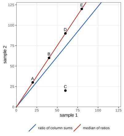
Algorithm 8.1 (median-of-ratios size factors; Anders and Huber 2010) Section 8.4.2, Question 8.1
- For each gene compute the geometric mean across samples, \(g_i=\big(\prod_{j=1}^mK_{ij}\big)^{1/m}\): a pseudo-reference sample. Genes with a zero in any sample have \(g_i=0\) and are dropped.
- For each sample \(j\), compute the ratios \(K_{ij}/g_i\) over the remaining genes.
- Set \(\hat s_j=\median_i\,K_{ij}/g_i\).
On the pasilla data, 9,063 of the 14,599 genes have no zero and are used; the course implementation agrees with DESeq2's estimateSizeFactorsForMatrix to machine precision.
Filling the gap 8.3: why the median of ratios is the right estimator, and when it fails Section 8.4.2 ("we can do better")
The book says the red line in Figure 8.1 "can be obtained by robust regression". Here is the model behind that statement and the properties that make the estimator robust.
Derivation
Model. Suppose that for the genes that do not change between samples, \(K_{ij}\approx s_jq_i\) up to noise, while a minority \(D\) of genes is differentially expressed. Then for an unchanged gene,
\[ \log K_{ij}-\frac1m\sum_{j'}\log K_{ij'}=\log s_j-\overline{\log s}+\varepsilon_{ij}, \qquad \overline{\log s}=\frac1m\sum_{j'}\log s_{j'}, \]where \(\varepsilon_{ij}\) is the centred log-noise. The gene-specific \(q_i\) has cancelled. So, for each sample, the left-hand side over genes is a sample of "location \(\log s_j-\overline{\log s}\) plus noise", contaminated by the genes in \(D\). Estimating a location from a contaminated sample is exactly what the median does well: \(\log\hat s_j=\median_i(\log K_{ij}-\log g_i)\), i.e. \(\hat s_j=\median_iK_{ij}/g_i\) (the median commutes with the monotone map \(\exp\)). This is least absolute deviations regression through the origin on the log scale, the robust regression the book alludes to.
Identifiability. Only ratios \(s_j/s_{j'}\) matter: multiplying all \(s_j\) by \(c\) and dividing all \(q_i\) by \(c\) leaves \(\mu_{ij}\) unchanged. The construction fixes the scale so that \(\prod_j\hat s_j\approx1\) (exactly 1 if the medians are taken over the same genes and there is no noise), so size factors scatter around 1.
Robustness. (i) A single gene changed by any factor moves \(\hat s_j\) by at most one order statistic of the ratios: multiplying one count by \(10^6\) moves the size factor by 0.02%, while the column sum grows about eightfold. (ii) The median's breakdown point is \(1/2\): as long as fewer than half the genes are changed, and the noise is symmetric, \(\hat s_j\) stays bounded. (iii) Changes that are balanced (as many genes up as down by similar amounts) leave the median of the log ratios nearly unchanged even when the changed genes are numerous, which is the relaxation of the few-changes assumption the book mentions in Section 8.6.1.
Failure mode. If a large fraction of genes changes in one direction, the median moves with them. If 30% of the genes are multiplied by 4 in one sample, the ratio of the two affected size factors is then inflated by a factor of 1.15, so every unchanged gene in that sample appears down-regulated by about 15%. The remedy is the one of Section 8.6.1: compute the medians over a set of control genes (or spike-ins) believed not to change.
Why the geometric mean. It is the reference that makes the log-ratio invariant to gene effects: any reference of the form \(\prod_jK_{ij}^{w_j}\) with \(\sum_jw_j=1\) would cancel \(q_i\), and equal weights treat the samples symmetrically. Its drawback is that a single zero removes the gene; with very sparse data (single cells) other estimators are needed. ∎
Question 8.1 (size factors versus column sums for pasilla) Section 8.4.2
For the pasilla count table, compare the median-of-ratios size factors with the column sums.
Answer
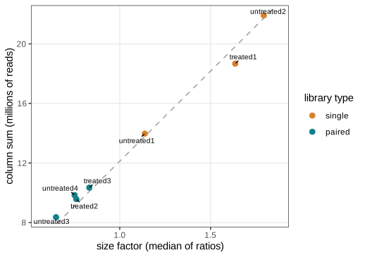
Figure 8.2 plots them. They are nearly proportional (the dashed line is a least-squares fit through the origin): for these data, the high-count genes behave like the bulk, so the cheap and the robust estimator agree up to a constant. The two single-end libraries with many lanes (untreated2 and treated1) are the deepest. The size factors are \(1.14, 1.79, 0.65, 0.75, 1.64, 0.76, 0.83\) for untreated1–4 and treated1–3.
Question 8.2 (mean-variance relationship) Section 8.4.2
Plot the variance against the mean of the normalised counts of the four untreated replicates.
Answer
Figure 8.3 shows \(\log\) variance against \(\log\) mean. The green line (slope 1, \(v=m\)) is the Poisson prediction and fits the low-count genes; the red line (slope 2, \(v=m^2\)) has the slope of the high-count genes, which lie below it, so \(v\approx cm^2\) with \(c<1\) there. The dashed blue curve is the gamma-Poisson relation \(v=m+\alpha(m)m^2\) with the fitted trend \(\alpha(m)=a_0+a_1/m\) of Section 8.10.1: it passes through the middle of the cloud over the whole range. Filling the gap 8.4 explains the two slopes.
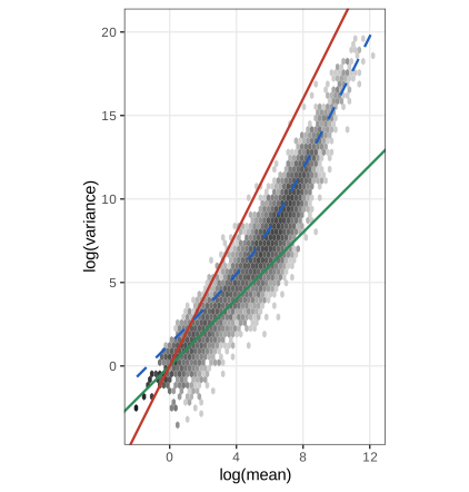
~ condition fit, \(a_0=0.0140\), \(a_1=2.72\). Reproduces Holmes and Huber (2019), Figure 8.3. Download: PDF · SVGFilling the gap 8.4: reading the slopes of Figure 8.3 Question 8.2
Derivation
Under the gamma-Poisson model a normalised count \(K_j/s_j\) of a gene with abundance \(q\) has mean \(q\) and variance \(\var(K_j)/s_j^2\)
On the log-log scale \(\log\E v=\log q+\log\big(\overline{s^{-1}}+\alpha q\big)\). For \(\alpha q\ll\overline{s^{-1}}\) this is \(\log q+\const\): slope 1, the Poisson regime (offset \(\log\overline{s^{-1}}\), which is close to 0 because the size factors scatter around 1). For \(\alpha q\gg\overline{s^{-1}}\) it is \(2\log q+\log\alpha\): slope 2 with intercept \(\log\alpha<0\), which is the book's "\(v=cm^2\) for some \(c<1\)" with \(c=\alpha\). The cross-over is at \(q\approx1/\alpha\): about 70 reads for a typical high-count dispersion \(\alpha\approx0.014\). Two practical consequences: (i) the size factors enter the variance (the dispersion is a property of the raw counts, which is why DESeq2 fits the model to raw counts with \(s_j\) as an offset rather than to normalised counts); (ii) a gene-wise variance from 4 replicates has a relative standard error of about \(\sqrt{2/3}\approx0.8\) (for normal data), visible as the vertical spread of the cloud, which motivates sharing information across genes. ∎
8.5 A basic analysis
8.5.1 Example dataset: the pasilla data
The sample annotation of the pasilla package records, for each library, the condition (untreated or treated, i.e. control or siRNA against pasilla) and the sequencing type: three libraries were sequenced single-end and four paired-end, in two batches. Cross-tabulating the two factors gives
| single | paired | |
|---|---|---|
| untreated | 2 | 2 |
| treated | 1 | 2 |
so the nuisance factor type is nearly, but not exactly, balanced against the factor of interest. The counts and the annotation are combined in a DESeqDataSet, a SummarizedExperiment that keeps the count matrix, the sample table (colData), the gene table (rowData) and the design formula together, so that subsetting one subsets all. The design formula of the first analysis is ~ condition.
Question 8.3 (row metadata of a SummarizedExperiment) Section 8.5.1
How are the row (gene) annotations of a SummarizedExperiment read and changed?
Answer
rowData(x) returns a DataFrame with one row per gene; rowData(x) <- df or rowData(x)$symbol <- v replaces it or adds a column (it must have nrow(x) rows in the same order). After DESeq(), the per-gene results of the fit (base mean, dispersions, coefficients, standard errors, convergence flags) are stored there too and are reached by mcols(x), a synonym. For ranged annotation (genomic coordinates) use rowRanges(x).
8.5.2 The DESeq2 method
DESeq() runs three steps: estimateSizeFactors (Algorithm 8.1), estimateDispersions (Section 8.10.1, Algorithm 8.3) and nbinomWaldTest (the GLM fit of Section 8.8 with a Wald test, Algorithm 8.2). The model it fits for each gene is (8.11) below; for the design ~ condition the coefficient of interest is the \(\log_2\) fold change between treated and untreated. The genes with the smallest adjusted p-values are
| gene | baseMean | log2 fold change | lfcSE | Wald z | p-value |
|---|---|---|---|---|---|
| FBgn0039155 | 730.6 | −4.619 | 0.1687 | −27.38 | 4.9e−165 |
| FBgn0025111 | 1501.4 | 2.900 | 0.1269 | 22.85 | 1.5e−115 |
| FBgn0029167 | 3706.1 | −2.197 | 0.0970 | −22.65 | 1.3e−113 |
| FBgn0003360 | 4343.0 | −3.180 | 0.1435 | −22.15 | 9.6e−109 |
(identical to the book's output). The baseMean is the mean of the normalised counts \(K_{ij}/\hat s_j\) over all samples; lfcSE is the standard error of the \(\log_2\) fold change; the Wald statistic is their ratio. The course's own IRLS fit (Algorithm 8.2) reproduces the fold changes and standard errors of 20 genes to \(10^{-6}\).
8.5.3 Exploring the results
Four plots are the first quality checks after a differential analysis: the p-value histogram, the MA plot, a PCA of the samples and a heatmap of the top genes.
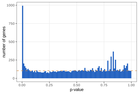
The histogram is a mixture of a flat component (null genes, whose p-values are uniform) and a peak near zero (genes that change). The first bin holds 993 genes and the background is about 100 per bin, so, as the book says, calling the whole first bin significant would have a false discovery rate of roughly \(100/993\approx10\%\). The reasoning is made exact next.
Filling the gap 8.5: the FDR read off a p-value histogram, and BH with independent filtering Section 8.5.3
Derivation
Two-groups model. Let a fraction \(\pi_0\) of the \(n\) tested genes be null, with p-values \(\mathrm{U}(0,1)\), and the rest have p-values with some density \(f_1\) concentrated near 0. The density of all p-values is \(f(p)=\pi_0+(1-\pi_0)f_1(p)\). If \(f_1(p)\approx0\) for \(p\) away from 0, the histogram height there estimates \(n\pi_0\times\)(bin width): here \(n\pi_0\cdot0.01\approx100\), i.e. \(\hat\pi_0\approx10{,}300/12{,}359\approx0.83\). Calling all genes with \(p\le t\) significant, the expected number of false calls is \(n\pi_0t\) and the number of calls is \(R(t)=\#\{p_i\le t\}\), so
\[ \widehat{\mathrm{FDR}}(t)=\frac{n\hat\pi_0\,t}{R(t)},\qquad\widehat{\mathrm{FDR}}(0.01)=\frac{103}{993}\approx0.10. \]Benjamini-Hochberg. With \(\hat\pi_0\) replaced by 1 (a conservative choice) and \(t\) chosen as the largest \(p_{(k)}\) with \(np_{(k)}/k\le q\), this is the BH procedure (Chapter 6 of the book proves that it controls the FDR at level \(\pi_0q\le q\) for independent p-values). The adjusted p-value of the \(k\)-th smallest p-value is \(\min_{l\ge k}np_{(l)}/l\), and a gene is called at level \(q\) when its adjusted p-value is at most \(q\).
Independent filtering. DESeq2 does not apply BH to all genes: it first removes genes with a small mean of normalised counts, which have almost no power, and applies BH to the rest; the cut-off is chosen to maximise the number of rejections. For pasilla it is a base mean of 6.56 (the 43% quantile), which is why padj is NA for 4,035 low-count genes. The filter is legitimate because, for a null gene, the base mean (computed ignoring the condition labels) is approximately independent of the p-value, so the p-values that survive the filter are still uniform under the null (Bourgon, Gentleman and Huber 2010). Recomputing padj as BH on the genes with base mean above the threshold matches DESeq2 to \(10^{-12}\). ∎
The book's footnote notes small spikes in the right half of the histogram. They come from genes with very small counts: their test statistic takes only a few values, so their p-values pile up at a few points, and they are exactly the genes removed by independent filtering.
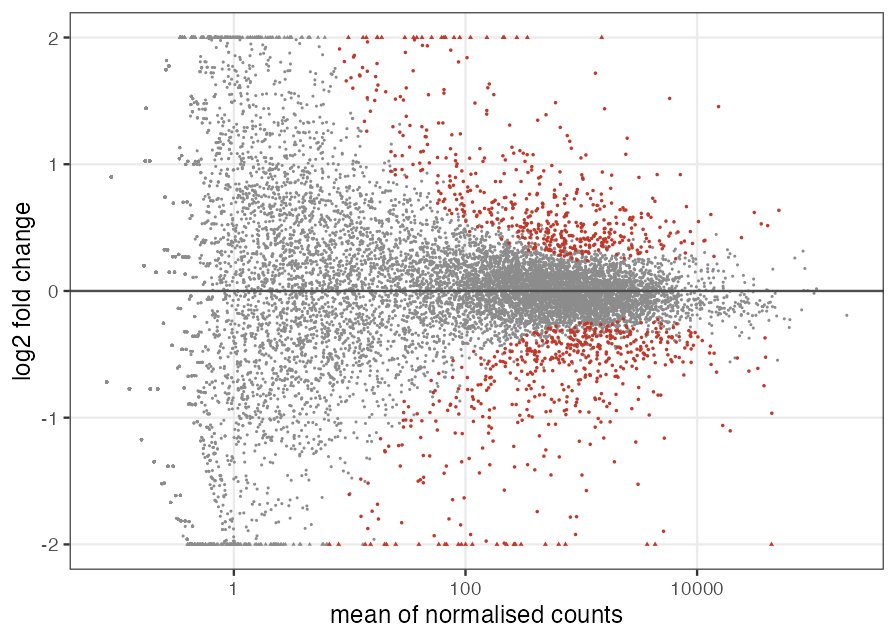
The name comes from microarrays: \(M\) is the log ratio (minus) and \(A\) the average log intensity. To make PCA and heatmaps meaningful the counts are first transformed to a scale on which the variance no longer depends strongly on the mean; the book uses the regularised logarithm (rlog), defined in Section 8.10.2.
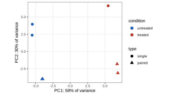
prcomp and matches plotPCA exactly. Reproduces Holmes and Huber (2019), Figure 8.6. Download: PDF · SVGQuestion 8.4 (must principal axes align with known covariates?) Section 8.5.3
Answer
No. PCA finds the directions of largest variance in the data, whatever causes them; it knows nothing about the design. When the leading axes align with the design, as here, the experimental factors are the main sources of variation, which is reassuring. When they do not, the leading axes reflect something else: an undocumented batch, a sample swap, RNA degradation, cell-cycle or composition differences, or a single outlying sample. That is a reason to investigate (and perhaps to add a blocking factor, Question 8.11), not a contradiction. Conversely, an effect of interest that is real but small can be invisible in the first two components and still be detected by a gene-wise test.
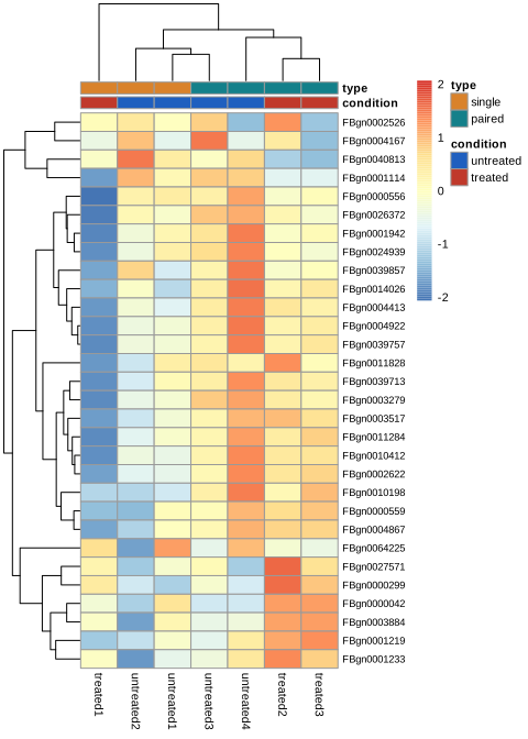
The book's Task asks for the same heatmap for the 30 most variable genes. On the rlog scale the most variable genes are those with large fold changes between conditions (the top hits of the test) and a few genes driven by one sample; their columns cluster by condition rather than by type. On the raw scale the most variable genes would simply be the most highly expressed ones, because the variance grows like \(\mu^2\): that is exactly the dependence a variance-stabilising transformation removes.
8.5.4 Exporting the results
The results table converts to a data frame and can be written as CSV (write.csv(as.data.frame(res), ...)); HTML reports with sortable tables can be generated by the ReportingTools package.
8.6 Critique of default choices and possible modifications
8.6.1 The few changes assumption
Both the median-of-ratios size factors and the dispersion trend use all genes, and both assume that most genes do not change. For the size factors, Filling the gap 8.3 shows that the weaker condition "changes are balanced around zero" suffices; for the dispersion trend it does not, because a gene with a real condition effect fitted with the right design does not inflate its dispersion, but a design that omits a strong factor does. When the assumption is doubtful (a global shift in transcription, a knock-down of a general factor), size factors should be computed from control genes or external spike-ins: estimateSizeFactors(dds, controlGenes = idx), which applies Algorithm 8.1 to the rows idx only.
8.6.2 Point-like null hypothesis
The default null hypothesis \(\beta=0\) says the fold change is exactly zero. With enough replicates almost every gene rejects it, because many genes respond weakly and indirectly. Testing against an interval, \(|\beta|\le\theta\), asks instead whether the change exceeds a biologically relevant size; Section 8.10.4 derives these tests.
8.7 Multi-factor designs and linear models
8.7.1 What is a multifactorial design?
Suppose cells are treated with an siRNA (\(x_1=1\)) or not (\(x_1=0\)), and with a drug (\(x_2=1\)) or not (\(x_2=0\)), in all four combinations. On a logarithmic scale the expression \(y\) of a gene is modelled as
\[ y=\beta_0+x_1\beta_1+x_2\beta_2+x_1x_2\beta_{12}. \tag{8.1} \]Reading the four cells: control \(y=\beta_0\); siRNA only \(y=\beta_0+\beta_1\); drug only \(y=\beta_0+\beta_2\); both \(y=\beta_0+\beta_1+\beta_2+\beta_{12}\). So \(\beta_1\) is the \(\log\) fold change of the siRNA,
\[ \beta_1=\log_2(\text{expression}_\text{siRNA})-\log_2(\text{expression}_\text{control})=\log_2\frac{\text{expression}_\text{siRNA}}{\text{expression}_\text{control}}, \tag{8.2} \]\(\beta_2\) that of the drug, and the interaction
\[ \beta_{12}=y_{11}-(\beta_0+\beta_1+\beta_2) \tag{8.3} \]is the departure of the combined treatment from additivity on the log scale (from multiplicativity on the original scale). Two biological scenarios from the book: if siRNA and drug hit the same target, \(\beta_1=\beta_2\) and the combination adds nothing, so \(y_{11}=\beta_0+\beta_1\) and \(\beta_{12}=-\beta_2=-\beta_1\); if they hit redundant parallel pathways, \(\beta_1,\beta_2\) are small and \(\beta_{12}\) large (synergy). The design matrix collects one row per experimental condition and one column per coefficient (with \(x_0=1\) for the intercept):
\[ \begin{array}{c|c|c|c} x_0 & x_1 & x_2 & x_1x_2\\ \hline 1&0&0&0\\ 1&1&0&0\\ 1&0&1&0\\ 1&1&1&1\end{array} \tag{8.4} \](The book prints (8.4) with the first three columns only, i.e. the design matrix of the additive model; the interaction model needs the fourth column \(x_1x_2\) as well. Without the combination experiment only the first three rows exist, and then the interaction cannot be estimated at all.)
Filling the gap 8.6: design matrices, identifiability and contrasts Sections 8.7.1–8.7.2, (8.4), (8.7)
Derivation
Cell means. Let \(\bm\mu=(\mu_{00},\mu_{10},\mu_{01},\mu_{11})^\T\) be the four cell means and \(\X_4\) the \(4\times4\) matrix (8.4) with the interaction column. Then \(\bm\mu=\X_4\bb\), and \(\X_4\) is lower triangular with unit diagonal, hence invertible: the interaction model is a one-to-one reparametrisation of the four cell means,
\[ \beta_0=\mu_{00},\quad\beta_1=\mu_{10}-\mu_{00},\quad\beta_2=\mu_{01}-\mu_{00},\quad\beta_{12}=(\mu_{11}-\mu_{01})-(\mu_{10}-\mu_{00}). \]The interaction is a difference of differences: the siRNA effect in the presence of the drug minus the siRNA effect without it. Dropping the interaction column imposes the single linear constraint \(\beta_{12}=0\) on the cell means.
Identifiability. With replicates, the \(m\times p\) design matrix \(\X\) has one row per sample (rows repeated for replicates). The coefficients are identifiable exactly when \(\X\) has full column rank \(p\), i.e. \(\X\bb=\X\bb'\Rightarrow\bb=\bb'\). For factors, R's default treatment coding drops the indicator of the reference level (the first level, here "untreated" and "single", which is why the levels were reordered); keeping all indicators plus an intercept would make the columns linearly dependent. A factor with \(L\) levels contributes \(L-1\) columns, so a paired design with 10 cell lines (Question 8.10) contributes 9 columns.
Contrasts. Any linear combination \(\mathbf{c}^\T\bb\) of the coefficients is a contrast and is estimated by \(\mathbf{c}^\T\hat\bb\) with variance \(\mathbf{c}^\T\cov(\hat\bb)\mathbf{c}\). In DESeq2, results(dds, contrast = c("type", "single", "paired")) builds \(\mathbf{c}\) so that the reported fold change is single over paired; with treatment coding and reference level "single" this is \(\mathbf{c}=(0,-1,0)^\T\) in the coefficients (Intercept, typepaired, conditiontreated), i.e. the negative of the typepaired coefficient. The book's output shows exactly this sign flip relative to the type_paired_vs_single coefficient. ∎
8.7.2 What about noise and replicates?
With replicate \(j\) and a residual \(\varepsilon_j\),
\[ y_j=x_{j0}\beta_0+x_{j1}\beta_1+x_{j2}\beta_2+x_{j1}x_{j2}\beta_{12}+\varepsilon_j, \tag{8.5} \]and the coefficients are chosen to make the residuals small, classically by least squares:
\[ \sum_j\varepsilon_j^2\ \to\ \min. \tag{8.6} \]Writing \(x_{j3}=x_{j1}x_{j2}\) and \(\beta_3=\beta_{12}\) puts (8.5) in the generic form
\[ y_j=\sum_kx_{jk}\beta_k+\varepsilon_j,\qquad\text{i.e.}\quad\mathbf{y}=\X\bb+\bm\varepsilon. \tag{8.7} \]Question 8.5 (the interaction term in the generic notation) Section 8.7.2
Answer
The sum in (8.7) runs over \(k=0,1,2,3\) with \(x_{j3}:=x_{j1}x_{j2}\) and \(\beta_3:=\beta_{12}\). A linear model is linear in the coefficients, not in the original variables, so any fixed function of the covariates (a product, a square, a spline basis) is just another column of \(\X\). All the scientific content of the model sits in the design matrix.
Filling the gap 8.7: least squares, its residuals, and the normal likelihood (8.6), Task in Section 8.7.2, Question 8.7
Derivation
Normal equations. \(S(\bb)=\|\mathbf{y}-\X\bb\|^2\) has gradient \(-2\X^\T(\mathbf{y}-\X\bb)\) and Hessian \(2\X^\T\X\), which is positive definite when \(\X\) has full column rank. So \(S\) is strictly convex and has the unique minimiser
\[ \hat\bb=(\X^\T\X)^{-1}\X^\T\mathbf{y},\qquad\hat{\bm\varepsilon}=\mathbf{y}-\X\hat\bb=(\mathbf{I}-\mathbf{H})\mathbf{y},\quad\mathbf{H}=\X(\X^\T\X)^{-1}\X^\T. \]Residuals average to zero (the book's Task), provided there is an intercept. The normal equations say \(\X^\T\hat{\bm\varepsilon}=\mathbf{0}\): the residuals are orthogonal to every column of \(\X\). If the first column is \(\mathbf{1}\) (the intercept, \(x_{j0}=1\)), the first equation is \(\sum_j\hat\varepsilon_j=0\). Without an intercept (and without a set of columns whose span contains \(\mathbf{1}\), such as all indicators of one factor) the residual mean need not vanish. In designs made only of factors, orthogonality to each indicator column means more: the residuals average to zero within every level of every factor in the model.
Least squares is maximum likelihood under normal errors (Question 8.7). With \(\varepsilon_j\) independent \(\N(0,\sigma^2)\) as in (8.9),
\[ \log\prod_jp(\varepsilon_j)=-\frac m2\log(2\pi\sigma^2)-\frac1{2\sigma^2}\sum_j(y_j-\mathbf{x}_j^\T\bb)^2, \]and for any fixed \(\sigma\) this is a decreasing function of the sum of squares, so (8.10) and (8.6) have the same maximiser \(\hat\bb\). Maximising over \(\sigma^2\) afterwards gives \(\hat\sigma^2_\text{ML}=S(\hat\bb)/m\); the unbiased estimator divides by the residual degrees of freedom \(m-p\) instead.
Sampling distribution. Under the normal model \(\hat\bb\sim\N(\bb,\sigma^2(\X^\T\X)^{-1})\), \(S(\hat\bb)/\sigma^2\sim\chi^2_{m-p}\) independently of \(\hat\bb\) (Cochran's theorem: \(\mathbf{I}-\mathbf{H}\) is a projection of rank \(m-p\) orthogonal to the column space), and \(t=(\hat\beta_k-\beta_k)/(\hat\sigma\sqrt{[(\X^\T\X)^{-1}]_{kk}})\sim t_{m-p}\). These are the tests used in Exercise 8.1. We verify that the residual mean is 0 and that numerical maximisation of the normal likelihood returns the least-squares coefficients. ∎
8.7.3 Analysis of variance
Why fit (8.5) instead of averaging replicates within each condition? With equal replicate numbers and only categorical factors both give the same cell means; the model earns its keep with unbalanced designs, continuous covariates and blocking factors, and it organises the variability of \(y\) into a sum of parts: a part explained by each factor and an unexplained part, the noise. Which part counts as noise depends on the model, not on the biology.
Filling the gap 8.8: the analysis of variance as a sum of orthogonal projections Section 8.7.3
Derivation
Let \(\mathcal{C}_0\subset\mathcal{C}_1\subset\dots\subset\mathcal{C}_K\) be the column spaces of a nested sequence of design matrices (intercept; plus factor 1; plus factor 2; plus the interaction), with orthogonal projections \(\mathbf{H}_0,\dots,\mathbf{H}_K\). Then
\[ \mathbf{y}-\mathbf{H}_0\mathbf{y}=\sum_{k=1}^K(\mathbf{H}_k-\mathbf{H}_{k-1})\mathbf{y}+(\mathbf{I}-\mathbf{H}_K)\mathbf{y}, \]and the terms are mutually orthogonal (each \(\mathbf{H}_k-\mathbf{H}_{k-1}\) projects onto \(\mathcal{C}_k\ominus\mathcal{C}_{k-1}\)). Pythagoras gives the ANOVA decomposition
\[ \|\mathbf{y}-\bar y\mathbf{1}\|^2=\sum_{k=1}^K\|(\mathbf{H}_k-\mathbf{H}_{k-1})\mathbf{y}\|^2+\|(\mathbf{I}-\mathbf{H}_K)\mathbf{y}\|^2, \]total sum of squares = one "sequential" sum of squares per term + residual sum of squares, with degrees of freedom \(d_k=\dim\mathcal{C}_k-\dim\mathcal{C}_{k-1}\) and \(m-\dim\mathcal{C}_K\). Under normal errors and the null hypothesis that term \(k\) has no effect, the ratio \(F_k=\big(\mathrm{SS}_k/d_k\big)\big/\big(\mathrm{RSS}/(m-p)\big)\) has an \(F(d_k,m-p)\) distribution. In balanced factorial designs the subspaces for the different factors are orthogonal and the sums of squares do not depend on the order in which terms enter; in unbalanced designs (like pasilla, 2/2 against 1/2) they do, which is one reason why the book prefers to speak of the fitted model and its coefficients. ∎
8.7.4 Robustness
Least squares has a breakdown point of \(1/m\): moving one observation far enough moves the fit arbitrarily far. The median, which minimises \(\sum_j|y_j-\beta_0|\), has breakdown point \(1/2\). Holmes and Huber (2019) list four robust alternatives to (8.6):
\[ \begin{aligned} R&=\textstyle\sum_j|\varepsilon_j| &&\text{least absolute deviations}\\ R&=\textstyle\sum_j\rho_s(\varepsilon_j) &&\text{M-estimation}\\ R&=Q_\theta\big(\{\varepsilon_1^2,\varepsilon_2^2,\dots\}\big) &&\text{LTS, LQS}\\ R&=\textstyle\sum_jw_j\varepsilon_j^2 &&\text{weighted regression}\end{aligned} \tag{8.8} \]Question 8.6 (Huber's loss) Section 8.7.4
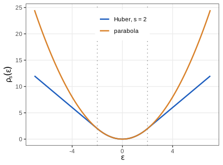
Plot Huber's (1964) function
\[ \rho_s(\varepsilon)=\begin{cases}\tfrac12\varepsilon^2,&|\varepsilon|<s,\\ s|\varepsilon|-\tfrac12s^2,&|\varepsilon|\ge s.\end{cases} \]Answer
Figure 8.8. The two pieces and their first derivatives agree at \(|\varepsilon|=s\) (value \(s^2/2\), slope \(\pm s\)), so \(\rho_s\) is convex and continuously differentiable; its derivative \(\psi_s(\varepsilon)=\max(-s,\min(s,\varepsilon))\) is the residual clipped at \(\pm s\). Beyond \(s\) the loss grows linearly, so a large residual exerts a bounded pull.
Filling the gap 8.9: M-estimation, its IRLS algorithm and breakdown points Section 8.7.4, (8.8)
Derivation
Estimating equations. For a convex differentiable \(\rho\) with \(\psi=\rho'\), the M-estimator minimises \(\sum_j\rho\big((y_j-\mathbf{x}_j^\T\bb)/\hat\sigma\big)\), where \(\hat\sigma\) is a robust scale such as \(\median_j|\hat\varepsilon_j|/0.6745\) (the factor makes it consistent for \(\sigma\) under normal errors, since the median of \(|Z|\) is \(\Phi^{-1}(0.75)=0.6745\)). Setting the gradient to zero,
\[ \sum_j\psi(u_j)\,\mathbf{x}_j=\mathbf{0},\qquad u_j=\frac{y_j-\mathbf{x}_j^\T\bb}{\hat\sigma}. \]IRLS. Write \(\psi(u)=w(u)\,u\) with weight \(w(u)=\psi(u)/u\); for Huber's function \(w(u)=\min(1,s/|u|)\). The equations become \(\sum_jw_j(y_j-\mathbf{x}_j^\T\bb)\mathbf{x}_j=\mathbf{0}\), the normal equations of weighted least squares with weights \(w_j\). Freezing the weights at the current fit and solving gives the update \(\bb\leftarrow(\X^\T\W\X)^{-1}\X^\T\W\mathbf{y}\), \(\W=\diag(w_j)\); then recompute the residuals, the scale and the weights. For convex \(\rho\) with \(w\) non-increasing in \(|u|\) each step does not increase the objective (it minimises a quadratic majoriser of \(\rho\) that touches it at the current residuals), so the iteration converges to the M-estimate. This is the fourth line of (8.8) with data-driven weights, and it is the algorithm of MASS::rlm: the course's 12-line implementation with \(s=1.345\) and MAD scale reproduces rlm on the mtcars data with one outlier to \(10^{-6}\).
Breakdown. For the mean, replacing one value by \(t\) moves the estimate by \((t-y_j)/m\to\infty\): breakdown point \(1/m\), i.e. 0 asymptotically. For the median of \(m\) values, the estimate stays inside the range of the unchanged values as long as fewer than half are replaced: breakdown \(\lfloor(m-1)/2\rfloor/m\to1/2\). Monotone M-estimators of regression (Huber) still have breakdown \(1/m\) against outliers in \(\mathbf{x}\) (leverage points), because their weights depend on the residual only; LTS (minimise the sum of the \(h\) smallest squared residuals, \(h\approx m/2\)) and least median of squares reach breakdown \(1/2\) at the price of a non-convex, combinatorial optimisation (Rousseeuw 1984). ∎
A note on the book's references. The book attributes least quantile of squares regression to "Rousseeuw 1987", but the entry with that label in its bibliography is Rousseeuw's paper on silhouettes for cluster analysis. The method was introduced in Rousseeuw (1984), and is treated at length in Rousseeuw and Leroy (1987).
All robust procedures involve a choice (\(s\), \(\theta\), the weights) that decides what counts as an outlier, and they need enough replicates to tell an outlier from a real effect. DESeq2 uses the fourth form of (8.8) with 0/1 weights set by Cook's distance (Section 8.10.3).
8.8 Generalized linear models
A linear model makes two assumptions: the mean of \(y\) is linear in the coefficients, and the errors are normal with constant variance (the justification of least squares). Generalised linear models (Nelder and Wedderburn 1972) relax both.
8.8.1 Modeling the data on a transformed scale
A probability or a mean count has a restricted range, while \(\mathbf{x}^\T\bb\) ranges over the real line. A link function \(g\) maps the mean into the real line, and the linear model is placed on that scale: \(g(\mu)=\mathbf{x}^\T\bb\). For probabilities the logit link, whose inverse is the logistic function \(1/(1+e^{-\eta})\) of Verhulst (1845), gives logistic regression; for counts the log link gives multiplicative effects, and fold changes become differences of coefficients.
8.8.2 Other error distributions
Least squares is maximum likelihood for normal residuals,
\[ p(\varepsilon_j)=\frac{1}{\sqrt{2\pi}\,\sigma}\exp\Big(-\frac{\varepsilon_j^2}{2\sigma^2}\Big), \tag{8.9} \] \[ \prod_jp(\varepsilon_j)\ \to\ \max \tag{8.10} \](Filling the gap 8.7), and the same likelihood principle applies to any other distribution. The useful class is the exponential family.
Question 8.7 (maximum likelihood and least squares) Section 8.8.2
Show that maximising (8.10) under (8.9) is the same as minimising (8.6).
Answer
Take logarithms: \(\log\prod_jp(\varepsilon_j)\)
Definition 8.3 (exponential dispersion family, GLM)
A density or pmf of the form
\[ f(y;\theta,\phi)=\exp\Big(\frac{y\theta-b(\theta)}{\phi}+c(y,\phi)\Big) \]is an exponential dispersion family with natural parameter \(\theta\), cumulant function \(b\) and dispersion parameter \(\phi\). A generalised linear model takes independent \(y_j\) from such a family with means \(\mu_j\) linked to the covariates by \(g(\mu_j)=\eta_j=\mathbf{x}_j^\T\bb+o_j\), where \(o_j\) is a known offset. The link with \(g(\mu)=\theta\) is canonical.
Filling the gap 8.10: mean, variance function, and the negative binomial as a GLM Section 8.8.2–8.8.3
Derivation
Moments. Differentiating \(\int f\,\d y=1\) with respect to \(\theta\) gives \(\int(y-b'(\theta))f\,\d y/\phi=0\), so \(\E y=b'(\theta)\). Differentiating again, \(\int\big[(y-b'(\theta))^2/\phi^2-b''(\theta)/\phi\big]f\,\d y=0\), so \(\var y=\phi\,b''(\theta)\). Writing \(V(\mu)=b''(\theta(\mu))\) for the variance function, \(\var y=\phi V(\mu)\).
Examples. Normal: \(\theta=\mu\), \(b=\theta^2/2\), \(\phi=\sigma^2\), \(V=1\). Poisson: \(f=\exp(y\log\mu-\mu-\log y!)\), so \(\theta=\log\mu\), \(b=e^\theta\), \(\phi=1\), \(V(\mu)=\mu\), and the log link is canonical.
Negative binomial with known \(\alpha\). From Result 8.1, with \(r=1/\alpha\),
\[ \log P(K=k)=k\log\frac{\mu}{r+\mu}+r\log\frac{r}{r+\mu}+\log\frac{\Gamma(k+r)}{\Gamma(r)k!}. \]So \(\theta=\log\frac{\mu}{r+\mu}\) (which is negative), \(\phi=1\), and since \(\frac{r}{r+\mu}=1-e^\theta\), \(b(\theta)=-r\log(1-e^\theta)\). Check: \(b'(\theta)=re^\theta/(1-e^\theta)=\mu\), and \(b''(\theta)=re^\theta/(1-e^\theta)^2\)
8.8.3 A generalized linear model for count data
The model fitted by DESeq2, gene by gene, is
\[ \begin{aligned} K_{ij}&\sim\GP(\mu_{ij},\alpha_i)\\ \mu_{ij}&=s_j\,q_{ij}\\ \log_2(q_{ij})&=\textstyle\sum_kx_{jk}\beta_{ik}. \end{aligned} \tag{8.11} \]The dispersion \(\alpha_i\) is specific to the gene and shared by its samples; the size factor \(s_j\) is specific to the sample and shared by its genes; the design matrix \((x_{jk})\) is common to all genes. Equivalently, \(\log\mu_{ij}=\log s_j+\ln2\cdot\mathbf{x}_j^\T\bb_i\): a GLM with log link and offset \(o_j=\log s_j\), whose coefficients are reported on the \(\log_2\) scale. (DESeq2 also allows gene- and sample-specific normalisation factors \(s_{ij}\), which change only the offset.)
Filling the gap 8.11: score equations and Fisher information for (8.11) Section 8.8.3
Derivation
Work with natural-log coefficients \(\bm b=\ln2\cdot\bb\) and drop the gene index. The log likelihood of one gene is \(\ell(\bm b)=\sum_j\log P(K_j=k_j;\mu_j,\alpha)\) with \(\log\mu_j=o_j+\mathbf{x}_j^\T\bm b\). From the pmf of Result 8.1,
\[ \frac{\partial\log P(K_j=k_j)}{\partial\mu_j}=\frac{k_j}{\mu_j}-\frac{k_j+r}{r+\mu_j}=\frac{k_j-\mu_j}{\mu_j(1+\alpha\mu_j)}=\frac{k_j-\mu_j}{V(\mu_j)}, \]and \(\partial\mu_j/\partial\bm b=\mu_j\mathbf{x}_j\). The score is therefore
\[ \mathbf{U}(\bm b)=\frac{\partial\ell}{\partial\bm b}=\sum_j\frac{k_j-\mu_j}{1+\alpha\mu_j}\,\mathbf{x}_j=\X^\T\W\,\mathbf{z}^\ast,\qquad w_j=\frac{\mu_j}{1+\alpha\mu_j},\ z^\ast_j=\frac{k_j-\mu_j}{\mu_j}. \]The MLE solves the score equations \(\mathbf{U}(\hat{\bm b})=\mathbf{0}\). For a general GLM the same computation gives \(\mathbf{U}=\sum_j\frac{(y_j-\mu_j)}{\phi V(\mu_j)g'(\mu_j)}\mathbf{x}_j\). The Fisher information is \(\mathcal{I}(\bm b)=\cov\mathbf{U}\)
Concavity. The observed information \(-\partial^2\ell/\partial\bm b\partial\bm b^\T=\sum_j\frac{\mu_j(1+\alpha k_j)}{(1+\alpha\mu_j)^2}\mathbf{x}_j\mathbf{x}_j^\T\) is positive semi-definite because every coefficient is positive; it is positive definite when \(\X\) has full rank. So \(\ell\) is strictly concave in \(\bm b\) and the MLE, when it exists, is unique. (It fails to exist when, for example, all counts of one group are zero: the coefficient then runs to \(-\infty\), which is why DESeq2 adds the tiny ridge penalty \(10^{-6}\beta^2/2\).)
The two-group case. With an intercept and a group indicator, the score equations say \(\sum_{j\in A}(k_j-\mu_j)/(1+\alpha\mu_j)=0\) for each group \(A\). If the size factors within a group are equal, the solution is \(\hat\mu_j=s_j\bar k_A/\bar s_A\) (group mean of the normalised counts); otherwise the MLE is a weighted compromise and must be computed iteratively. We verify that the course IRLS solution makes every score component smaller than \(10^{-6}\). ∎
Algorithm 8.2 (IRLS for the negative binomial GLM with offset) Section 8.8.3
- Start from \(\bm b^{(0)}\) (for example the least-squares fit of \(\log(k_j/s_j+0.1)\) on \(\X\)).
- Given \(\bm b^{(t)}\), compute \(\eta_j=\log s_j+\mathbf{x}_j^\T\bm b^{(t)}\), \(\mu_j=e^{\eta_j}\), weights \(w_j=\mu_j/(1+\alpha\mu_j)\) and the working response \(z_j=\eta_j-\log s_j+(k_j-\mu_j)/\mu_j\).
- Solve the weighted least-squares problem \(\bm b^{(t+1)}=(\X^\T\W\X+\bm\Lambda)^{-1}\X^\T\W\mathbf{z}\), with \(\bm\Lambda=\mathbf{0}\) for the MLE (DESeq2 uses \(\lambda=10^{-6}\) on the \(\log_2\) scale, i.e. \(\bm\Lambda=\diag(10^{-6}/(\ln2)^2)\)).
- Stop when the deviance changes by less than \(10^{-8}\) relative; report \(\hat\bb=\hat{\bm b}/\ln2\) and standard errors \(\sqrt{\diag\big(\X^\T\W\X\big)^{-1}}/\ln2\).
Filling the gap 8.12: why IRLS is Fisher scoring Section 8.8.3
Derivation
Fisher scoring replaces the Hessian in Newton's method by minus the expected information: \(\bm b^{(t+1)}=\bm b^{(t)}+\mathcal{I}^{-1}\mathbf{U}\). With \(\mathcal{I}=\X^\T\W\X\) and \(\mathbf{U}=\X^\T\W\mathbf{z}^\ast\) (Filling the gap 8.11),
\[ \bm b^{(t+1)}=(\X^\T\W\X)^{-1}\big(\X^\T\W\X\,\bm b^{(t)}+\X^\T\W\mathbf{z}^\ast\big)=(\X^\T\W\X)^{-1}\X^\T\W\big(\X\bm b^{(t)}+\mathbf{z}^\ast\big). \]Since \(\X\bm b^{(t)}=\bm\eta-\mathbf{o}\), the vector in brackets is the working response \(\mathbf{z}\) of step 2: each Fisher scoring step is a weighted least-squares regression of \(\mathbf{z}\) on \(\X\). The working response is a first-order expansion of the link at the current mean, \(g(k_j)\approx g(\mu_j)+g'(\mu_j)(k_j-\mu_j)\), with the offset removed, and \(w_j\) is the inverse of its approximate variance \(g'(\mu_j)^2\var(K_j)\). With the canonical link Fisher scoring and Newton-Raphson coincide; with the log link for the NB they differ (expected versus observed information), but both converge to the same unique maximiser. A ridge penalty \(\frac12\bm b^\T\bm\Lambda\bm b\) adds \(-\bm\Lambda\bm b\) to the score and \(\bm\Lambda\) to the information, giving step 3 with \(\bm\Lambda\).
Standard errors. At the MLE, \(\hat{\bm b}\approx\N\big(\bm b,\mathcal{I}(\hat{\bm b})^{-1}\big)\) (asymptotic normality of the MLE), and \(\hat\bb=\hat{\bm b}/\ln2\) has covariance \(\mathcal{I}^{-1}/(\ln2)^2\). With a ridge term DESeq2 reports the sandwich \((\X^\T\W\X+\bm\Lambda)^{-1}\X^\T\W\X(\X^\T\W\X+\bm\Lambda)^{-1}\), the covariance of the penalised estimator.
The course implementation of Algorithm 8.2 reproduces DESeq2's \(\log_2\) fold changes and standard errors to \(10^{-6}\) for 20 genes and both designs, and with \(\alpha\to0\) and no penalty it reproduces glm(family = poisson) with offset, including the deviance. Started from the least-squares fit of \(\log(k_j/s_j+0.1)\), the log likelihood increased at every step for the 20 genes tested. The starting value matters: from \(\bm b=\mathbf{0}\) the working response \((k_j-\mu_j)/\mu_j\approx k_j/s_j\) is in the thousands for a highly expressed gene, and the first step throws the intercept to about 1800 on the \(\log_2\) scale (Fisher scoring is only locally convergent for a non-canonical link). Conversely, DESeq2's own fit is not always at the maximum: for two low-count genes with very flat likelihoods (FBgn0037191 and FBgn0053498, the latter with all treated counts zero) its IRLS stops early, and the course fit reaches a log likelihood higher by 0.0005 and 0.32; the reported fold changes differ accordingly (4.227 against 4.190 for the first gene). ∎
Filling the gap 8.13: Wald test, likelihood ratio test and deviance Sections 8.5.2, 8.8.3 (the book defers the test to the papers)
Derivation
Wald test. For \(H_0:\beta_k=0\), the statistic \(z=\hat\beta_k/\widehat{\mathrm{SE}}(\hat\beta_k)\) is approximately \(\N(0,1)\) under \(H_0\) by asymptotic normality of the MLE, and the two-sided p-value is \(2\Phi(-|z|)\). For a contrast \(\mathbf{c}^\T\bb\), use \(\mathbf{c}^\T\hat\bb/\sqrt{\mathbf{c}^\T\widehat\cov(\hat\bb)\mathbf{c}}\). DESeq2's stat and pvalue columns are exactly these (checked to \(10^{-10}\) for all genes).
Likelihood ratio test. To test a reduced design \(\X_0\) (column space inside that of \(\X\), \(p_0<p\) columns) against \(\X\), with the dispersion held at the full model's estimate,
\[ \Lambda=2\big(\ell(\hat{\bm b})-\ell(\hat{\bm b}_0)\big)\ \approx\ \chi^2_{p-p_0}\quad\text{under }H_0. \]Proof sketch: expand \(\ell\) to second order around \(\hat{\bm b}\); the difference of the maximised quadratic forms is the squared length of the projection of a \(\N(\mathbf{0},\mathcal{I})\) score onto a \((p-p_0)\)-dimensional complement, which is \(\chi^2_{p-p_0}\) (Wilks' theorem). The Wald and LR statistics are asymptotically equivalent (\(z^2\approx\Lambda\) for one coefficient) but differ in small samples; the LRT is invariant to reparametrisation, the Wald test is not, and they disagree most for low counts and for coefficients near the boundary. An extreme case is a gene with all counts of one group equal to zero (FBgn0053498 in pasilla): the fold change estimate runs off towards \(-\infty\), its standard error grows even faster, and the Wald statistic goes to zero although the likelihood ratio statistic is clearly positive (the Hauck-Donner effect).
Deviance. The deviance of a fit is \(D=2(\ell_\text{sat}-\ell(\hat{\bm b}))\), where the saturated model sets \(\mu_j=k_j\); for the NB,
\[ D=2\sum_j\Big[k_j\log\frac{k_j}{\hat\mu_j}-(k_j+r)\log\frac{k_j+r}{\hat\mu_j+r}\Big], \]which for \(r\to\infty\) becomes the Poisson deviance \(2\sum_j[k_j\log(k_j/\hat\mu_j)-(k_j-\hat\mu_j)]\). Since \(\ell_\text{sat}\) does not depend on the model, \(\Lambda=D_0-D\). (DESeq2 stores \(-2\ell(\hat{\bm b})\) in its deviance column, which differs from \(D\) by the constant \(-2\ell_\text{sat}\).)
A detail found while checking. For the two-factor comparison ~ type + condition against ~ type, the course LRT matches DESeq2's nbinomLRT to \(10^{-5}\). Against the intercept-only model ~ 1, DESeq2 does not maximise the likelihood: it takes the intercept as \(\log_2\) of the mean normalised count, which is the MLE only when all size factors are equal (the intercept-only score equation is \(\sum_j(k_j-s_je^{b})/(1+\alpha s_je^b)=0\)). Its reduced log likelihood is therefore slightly too low and its LR statistic slightly too large (by up to 0.016 for the 20 genes checked, so its p-values are slightly too small; the effect matters only for genes near the significance threshold). ∎
8.9 Two-factor analysis of the pasilla data
The PCA (Figure 8.6) and the heatmap (Figure 8.7) show that the library type has a strong systematic effect. Adding it to the design, ~ type + condition, makes it a blocking factor (a nuisance factor whose effect is estimated and removed). By DESeq2's convention the variable of interest comes last, so that results() reports its coefficient by default; any other coefficient or contrast is obtained with the contrast argument, e.g. contrast = c("type", "single", "paired") for single-end over paired-end.
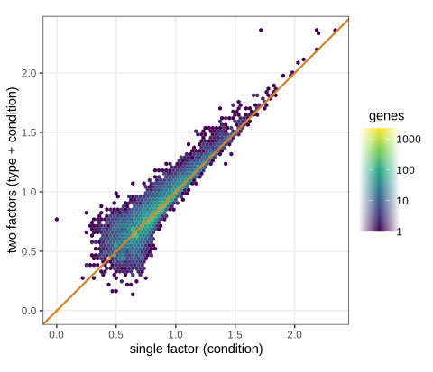
~ condition, \(x\)) against the two-factor analysis (~ type + condition, \(y\)), both shown as \((-\log_{10}p)^{1/6}\) (a decreasing transformation chosen only to compress the range). Points above the orange diagonal have smaller p-values in the two-factor analysis. Reproduces Holmes and Huber (2019), Figure 8.9. Download: PDF · SVGCross-tabulating the calls at adjusted p < 0.1:
| one-factor \ two-factor | not called | called | total |
|---|---|---|---|
| not called | 6973 | 289 | 7262 |
| called | 25 | 1036 | 1061 |
| total | 6998 | 1325 | 8323 |
The two-factor analysis gains about a quarter more discoveries. (A small point of bookkeeping: the table only counts genes whose adjusted p-value is defined in both analyses. Over all genes the two-factor analysis calls 1330, not 1325; the five extra genes were removed by independent filtering in the one-factor analysis.)
~ condition and ~ type + condition and see the standard error shrink.Question 8.8 (why the blocking factor gives more discoveries) Section 8.9
Answer
Without the blocking factor, the variation due to type is left in the residuals and inflates the noise; with it, that variation is explained, at the cost of one more parameter (one fewer residual degree of freedom) and, for unbalanced designs, a slightly larger design factor for the condition coefficient. Filling the gap 8.14 quantifies both effects for pasilla: the design factor grows by 3% while the typical dispersion drops by 43%, so the gain wins clearly. In general either effect can win.
Filling the gap 8.14: variance of a treatment effect with and without a blocking factor, and confounding Questions 8.8–8.9
Derivation
Normal linear model. Let \(\mathbf{c}\) be the condition indicator and \(\mathbf{Z}\) the other columns (intercept, blocks). By the Frisch-Waugh-Lovell theorem, \(\hat\beta_c\) equals the slope of \(\mathbf{y}\) on the residual \(\tilde{\mathbf{c}}=(\mathbf{I}-\mathbf{H}_Z)\mathbf{c}\), so
\[ \var\hat\beta_c=\frac{\sigma^2}{\|\tilde{\mathbf{c}}\|^2}. \]Adding blocks to \(\mathbf{Z}\) can only shrink \(\|\tilde{\mathbf{c}}\|^2\) (projecting onto a larger space removes more), and it is unchanged exactly when \(\mathbf{c}\) is balanced across blocks (orthogonal to the block indicators after centring). For pasilla, with intercept only, \(\|\tilde{\mathbf{c}}\|^2=4(3/7)^2+3(4/7)^2=12/7\), design factor \(7/12=0.583\); with type, centring within each type gives \(\|\tilde{\mathbf{c}}\|^2\)
The gain. In the one-factor model the residual variance is \(\sigma^2_\text{block}+\sigma^2\), where \(\sigma^2_\text{block}\) is the part of the variance explained by type. For the NB model the same thing happens on the dispersion scale: the fitted asymptotic dispersion \(a_0\) is 0.0140 with ~ condition and 0.0080 with ~ type + condition. Since \(\var\hat\beta_c\approx\frac{\text{design factor}}{(\ln2)^2}\big(\overline{1/\mu}+\alpha\big)\) for a gene in the high-count regime, the variance of a fold change drops by about 40% there, more than offsetting the loss of one residual degree of freedom.
Confounding (Question 8.9). If the true mean model contains \(\beta_t\mathbf{t}\) (type) but the fit omits it, then \(\E\hat\beta_c=\beta_c+\beta_t\delta\), where \(\delta\) is the slope of \(\mathbf{t}\) on \(\mathbf{c}\) (with an intercept): the omitted-variable bias. Here \(\delta=P(\text{paired}\given\text{treated})\)
Question 8.9 (confounding) Section 8.9
Answer
Two factors are confounded when their levels co-vary across the samples, so that their effects cannot be separated (fully) or can be separated only with a loss of precision (partially). Not modelling a confounded blocking factor biases the estimate of interest by \(\beta_t\delta\) (Filling the gap 8.14) and can therefore produce more, spurious, detections.
Question 8.10 (paired designs) Section 8.9
Ten cell lines, each measured with and without a drug: how should this be analysed?
Answer
Add the cell line as a blocking factor: design ~ cell + treatment, with cell a factor of 10 levels (9 columns). The treatment coefficient is then estimated from within-cell-line comparisons, and the (usually large) differences between cell lines leave the residual variance. The airway data (Himes et al. 2014) are such a design: four airway smooth muscle cell lines, each untreated and treated with dexamethasone. On the 22,369 genes with at least 10 reads, the paired analysis (~ cell + dex) calls 4834 genes at adjusted p < 0.1 against 3386 for the unpaired analysis (~ dex); 1540 genes are found only by the paired analysis and 95 only by the unpaired one (supplementary Figure S2).
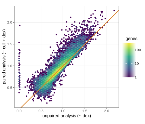
~ cell + dex) against the unpaired analysis (~ dex), on the same \((-\log_{10}p)^{1/6}\) scale as Figure 8.9. Blocking on the cell line moves most genes above the diagonal. Download: PDF · SVGQuestion 8.11 (hidden factors) Section 8.9
Answer
Estimate them from the data and add the estimates as covariates. Surrogate variable analysis (Leek and Storey 2007) takes the residuals of the model with the known factors and extracts their leading singular vectors (with a permutation-based selection of how many), then adds them to the design; factor-analysis methods such as PEER (Stegle et al. 2010) do the same within a Bayesian model. The danger is removing real biology: the surrogate variables must be estimated so that they are not correlated with the factor of interest, which is easiest when the design is balanced.
8.10 Further statistical concepts
8.10.1 Sharing of dispersion information across genes
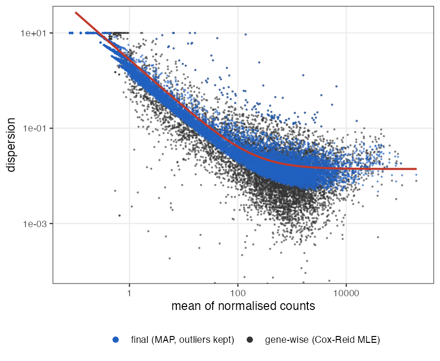
(The book says the dispersions are "the \(\alpha\)s in the third line of Equation 8.11"; they appear in the first line, \(K_{ij}\sim\GP(\mu_{ij},\alpha_i)\), while the third line holds the coefficients \(\beta_{ik}\).) With \(m=7\) samples and \(p=2\) coefficients, a gene-wise dispersion estimate rests on 5 residual degrees of freedom and is very noisy (supplementary Figure S1, grey points). DESeq2 shrinks each estimate towards a trend fitted across all genes, by an amount that depends on how informative the gene's own data are. The same empirical Bayes idea is applied, optionally, to the fold changes. The book refers to Love, Huber and Anders (2014) for the mathematics; here it is.
Algorithm 8.3 (DESeq2 dispersion estimation) Section 8.10.1; Love et al. (2014)
- Gene-wise estimates. For each gene, alternate: fit the means \(\mu_{ij}\) by Algorithm 8.2 at the current \(\alpha_i\); then maximise the Cox-Reid adjusted profile likelihood (Filling the gap 8.15) over \(\log\alpha_i\) with the means held fixed. Call the result \(\hat\alpha_i^\text{gw}\).
- Trend. Fit \(\alpha_\text{tr}(\bar\mu)=a_0+a_1/\bar\mu\) to the pairs \((\bar\mu_i,\hat\alpha_i^\text{gw})\), where \(\bar\mu_i\) is the base mean, by a gamma-family GLM with identity link, refitting after dropping genes whose ratio \(\hat\alpha^\text{gw}/\alpha_\text{tr}\) lies outside \((10^{-4},15)\). Pasilla: \(a_0=0.01396\), \(a_1=2.723\).
- Prior width. \(\sigma_d^2=\max(r_d,0.25)\) with \(r_d=\mathrm{mad}^2_i[\log\hat\alpha_i^\text{gw}\)
\({}-\log\alpha_\text{tr}(\bar\mu_i)]\) \({}-\psi_1\big(\tfrac{m-p}2\big)\), with \(\psi_1\) the trigamma function. Pasilla: \(0.9899-0.4904=0.4995\). - MAP. Maximise \(\ell_\text{CR}(\log\alpha)-\big(\log\alpha-\log\alpha_\text{tr}(\bar\mu_i)\big)^2/(2\sigma_d^2)\) over \(\log\alpha\): the posterior mode under the log-normal prior \(\log\alpha_i\sim\N(\log\alpha_\text{tr}(\bar\mu_i),\sigma_d^2)\).
- Outliers. If \(\log\hat\alpha_i^\text{gw}>\log\alpha_\text{tr}(\bar\mu_i)+2\sigma_d\), keep \(\hat\alpha_i^\text{gw}\) instead of the MAP (108 genes in pasilla): a gene whose data clearly contradict the prior is not pulled towards it, which would make it falsely significant.
The course code reproduces steps 2 and 3 exactly, and steps 1 and 4 to a relative error below \(10^{-3}\) (DESeq2 maximises with a line search of finite tolerance).
Filling the gap 8.15: the Cox-Reid adjusted profile likelihood Section 8.10.1
Maximising the likelihood jointly over \(\bb\) and \(\alpha\) underestimates \(\alpha\) when \(p\) is not small compared with \(m\), for the same reason that \(\mathrm{RSS}/m\) underestimates \(\sigma^2\). Cox and Reid (1987) correct the profile likelihood by a determinant term:
\[ \ell_\text{CR}(\alpha)=\ell\big(\hat\bb_\alpha,\alpha\big)-\tfrac12\log\det\big(\X^\T\W_\alpha\X\big),\qquad w_j=\frac{\mu_j}{1+\alpha\mu_j}. \]Derivation
Why a correction is needed. The profile likelihood \(\ell_P(\alpha)=\max_{\bb}\ell(\bb,\alpha)\) treats the fitted means as if they were known. But fitted means are closer to the data than the true means, so the residuals look too small and the dispersion is underestimated. In the normal linear model this is exact: \(\ell_P(\sigma^2)=-\frac m2\log\sigma^2-\mathrm{RSS}/(2\sigma^2)\), maximised at \(\mathrm{RSS}/m\), whose expectation is \(\sigma^2(m-p)/m\).
The Cox-Reid adjustment. If the nuisance parameter \(\bb\) is (made) orthogonal to the parameter of interest, the conditional likelihood of the data given \(\hat\bb_\alpha\) is approximated by \(\ell_P(\alpha)-\frac12\log\det\mathcal{I}_{\bb\bb}(\hat\bb_\alpha,\alpha)\), where \(\mathcal{I}_{\bb\bb}\) is the information for \(\bb\) at fixed \(\alpha\). The extra term penalises values of \(\alpha\) at which \(\bb\) is well determined, compensating the overfitting of the means. For the NB GLM, \(\mathcal{I}_{\bb\bb}=\X^\T\W\X\) (Filling the gap 8.11), and orthogonality holds: \(\E\,\partial^2\ell/\partial\bb\partial\alpha=0\) because \(\partial\ell/\partial\bb=\sum_j(k_j-\mu_j)\mathbf{x}_j/(1+\alpha\mu_j)\) has expectation 0 for every \(\alpha\), and so does its derivative in \(\alpha\).
Check in the normal case. There \(\mathcal{I}_{\bb\bb}=\X^\T\X/\sigma^2\), so \(-\frac12\log\det=\frac p2\log\sigma^2+\const\) and
\[ \ell_\text{CR}(\sigma^2)=-\frac{m-p}2\log\sigma^2-\frac{\mathrm{RSS}}{2\sigma^2}+\const,\qquad\hat\sigma^2_\text{CR}=\frac{\mathrm{RSS}}{m-p}, \]the unbiased (REML) estimator. For the NB the adjustment is not exactly unbiasing but removes most of the bias. The course implementation (cr_apl, disp_est) maximises \(\ell_\text{CR}\) over \(\log\alpha\) with Brent's method; with the fitted means of DESeq2's gene-wise step it reproduces dispGeneEst with median relative error \(3\times10^{-4}\) over 150 genes (genes with a very flat likelihood differ more, which is harmless because they are shrunk anyway). ∎
Filling the gap 8.16: the log-normal prior, its width, and how much the MAP shrinks Section 8.10.1
Derivation
Sampling variance of a log dispersion estimate. Use the normal analogue: a variance estimate with \(\nu=m-p\) degrees of freedom satisfies \(\hat\sigma^2=\sigma^2G/(\nu/2)\) with \(G\sim\Gam(\nu/2,1)\) (since \(\chi^2_\nu/2\sim\Gam(\nu/2,1)\)). For \(G\sim\Gam(a,1)\), \(\E G^t=\Gamma(a+t)/\Gamma(a)\), so the cumulant generating function of \(\log G\) is \(\log\Gamma(a+t)-\log\Gamma(a)\), and differentiating twice at \(t=0\),
\[ \var\log G=\psi_1(a),\qquad\text{hence}\qquad\var\log\hat\sigma^2=\psi_1\big(\tfrac{m-p}2\big). \]For \(m-p=5\), \(\psi_1(2.5)=0.490\) (a simulation confirms it). DESeq2 uses this as the sampling variance of \(\log\hat\alpha^\text{gw}\), treating the dispersion estimate like a variance estimate with \(m-p\) degrees of freedom.
Prior width by deconvolution. If \(\log\hat\alpha_i^\text{gw}=\log\alpha_i+e_i\) with \(e_i\) independent of \(\log\alpha_i\), and \(\log\alpha_i=\log\alpha_\text{tr}(\bar\mu_i)+d_i\) with \(\var d_i=\sigma_d^2\), then the residuals \(r_i=\log\hat\alpha_i^\text{gw}-\log\alpha_\text{tr}(\bar\mu_i)\) have variance \(\sigma_d^2+\psi_1((m-p)/2)\). DESeq2 estimates \(\var r_i\) robustly by the squared median absolute deviation (consistent for the variance under normality and insensitive to the dispersion outliers) and subtracts the sampling part. The floor 0.25 prevents a degenerate prior when the two terms nearly cancel.
How much shrinkage. Near its maximum the adjusted log likelihood in \(\theta=\log\alpha\) is roughly quadratic with curvature \(1/\psi_1\) (the inverse sampling variance). Adding the log prior, the posterior mode is the precision-weighted average
\[ \log\hat\alpha^\text{MAP}\approx\frac{\log\hat\alpha^\text{gw}/\psi_1+\log\alpha_\text{tr}/\sigma_d^2}{1/\psi_1+1/\sigma_d^2}. \]For the pasilla one-factor fit \(\psi_1=0.490\) and \(\sigma_d^2=0.500\): the weights are almost equal, so the final dispersion is close to the geometric mean of the gene-wise value and the trend. For the two-factor fit (\(m-p=4\), \(\psi_1(2)=0.645\), \(\sigma_d^2=0.255\)) the gene-wise estimate gets weight \(0.28\) only. For genes with low counts the likelihood is flatter than the normal analogue suggests and the prior dominates even more. Exactly (without the quadratic approximation) the MAP lies between the gene-wise estimate and the trend on the log scale, which holds for 150 genes; the course MAP reproduces dispMAP to a relative error of \(5\times10^{-4}\). ∎
Filling the gap 8.17: why the trend is \(a_0+a_1/\bar\mu\) and why it is fitted by a gamma GLM Section 8.10.1
Derivation
Form. Result 8.1 says \(\mathrm{CV}^2=1/\mu+\alpha\). If, besides biological variation with a constant squared coefficient of variation \(a_0\), there is technical noise whose variance is proportional to the mean (Poisson-like, e.g. from library preparation), with variance \(a_1\mu\), then \(\var K=\mu+a_1\mu+a_0\mu^2\), which is the NB variance with \(\alpha(\mu)=a_0+a_1/\mu\). So \(a_0\) is the asymptotic dispersion (biological CV\(^2\) of highly expressed genes, here \(\sqrt{0.014}\approx12\%\)) and \(a_1\) the "extra-Poisson" noise that dominates at low counts.
Gamma family, identity link. A dispersion estimate with \(\nu\) degrees of freedom is approximately \(\alpha\,\chi^2_\nu/\nu\), whose variance is \(2\alpha^2/\nu\): proportional to the square of its mean. That is the variance function \(V(\mu)=\mu^2\) of the gamma family, so a gamma GLM gives each gene the right weight. The link is the identity because the trend is linear in the coefficients \((a_0,a_1)\) with covariates \((1,1/\bar\mu)\). The course function disp_trend repeats DESeq2's iteration (refit after removing genes with ratios outside \((10^{-4},15)\)) and recovers its coefficients to machine precision. ∎
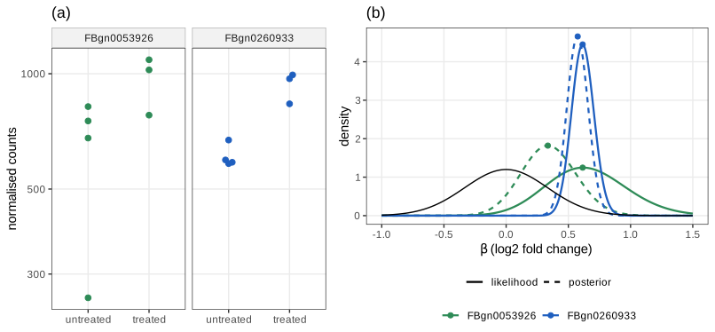
The same empirical Bayes construction applied to the fold changes gives shrunken \(\log_2\) fold changes. The prior is normal with mean 0; its variance is estimated from the distribution of the maximum likelihood fold changes over all genes. Figure 8.10 shows its effect on two genes with almost the same mean and the same MLE fold change (about 0.61) but very different dispersions.
Filling the gap 8.18: shrunken fold changes are ridge-penalised MLEs Section 8.10.1, Figure 8.10
Derivation
MAP = penalised likelihood. With prior \(\beta_k\sim\N(0,\sigma_\beta^2)\) on the non-intercept coefficients (\(\log_2\) scale) and a flat prior on the intercept, the log posterior is \(\ell(\bb)-\sum_{k\ge1}\beta_k^2/(2\sigma_\beta^2)\). Its maximiser is computed by Algorithm 8.2 with \(\lambda_k=1/\sigma_\beta^2\) on the \(\log_2\) scale (\(1/(\sigma_\beta^2(\ln2)^2)\) on the natural scale). The course implementation reproduces lfcShrink(type = "normal") to \(10^{-14}\): shrunken values 0.237 (green gene, MLE 0.617) and 0.544 (blue gene, MLE 0.614).
How much. If the log likelihood in \(\beta\) is quadratic, \(\ell\approx\const-(\beta-\hat\beta)^2/(2\,\mathrm{SE}^2)\), the posterior is normal with mode
\[ \beta^\text{MAP}=\frac{\sigma_\beta^2}{\sigma_\beta^2+\mathrm{SE}^2}\,\hat\beta. \]For the green gene \(\mathrm{SE}=0.425\) and the factor is \(0.1106/(0.1106+0.1803)=0.380\), giving \(0.235\); for the blue gene \(\mathrm{SE}=0.120\), factor \(0.885\), giving \(0.544\). Both agree with the exact values to the third decimal. The shrinkage is strong exactly when the data are uninformative (low counts or high dispersion), which is what makes shrunken fold changes good for ranking genes by effect size.
Prior variance. DESeq2 matches an upper quantile: it takes the 95% quantile \(q\) of \(|\hat\beta_i|\) over genes, weighted by \(1/(1/\bar\mu_i+\alpha_\text{tr}(\bar\mu_i))\) (the inverse of the approximate variance of a log count, so that noisy genes count less), and sets \(\sigma_\beta=q/z_{0.975}\), the normal whose absolute value has the same 95% quantile. For pasilla \(\sigma_\beta^2=0.1106\) (reproduced by the course function weighted_upper_var to \(10^{-14}\)). Matching a tail quantile rather than the variance makes the prior wide enough for the genuinely changed genes.
A remark on Figure 8.10(b). The book's curves (and ours) hold the intercept fixed at its MLE, so they are conditional likelihoods and posteriors. The DESeq2 estimate maximises over the intercept as well, i.e. it uses the profile, which is wider. The modes of the dashed curves (0.335 and 0.575 on the grid) are therefore not the shrunken values 0.237 and 0.544; the figure illustrates the mechanism, not the exact numbers. The likelihood maxima do coincide with the MLEs (checked to the grid step 0.005). ∎
8.10.2 Count data transformations
Tests use the raw counts and the NB model. For clustering, PCA, heatmaps and plots, a transformation to an approximately homoskedastic scale is convenient. The simplest is the shifted logarithm
\[ y=\log_2(n+1)\quad\text{or more generally}\quad y=\log_2(n+n_0), \tag{8.12} \]with a pseudocount \(n_0\). The book offers two better-founded choices.
Variance-stabilising transformation
A variance-stabilising transformation (VST) is a function \(g\) such that \(\var g(K)\) is approximately constant whatever the mean. DESeq2 computes it from the fitted dispersion trend (Anders and Huber 2010), usually "blind" to the design (dispersions re-estimated with ~ 1, here \(a_0=0.0221\), \(a_1=2.270\)).
Filling the gap 8.19: the VST of the gamma-Poisson model in closed form Section 8.10.2 (refers to Section 4.4.4)
Derivation
Delta method. If \(K\) has mean \(\mu\) and variance \(v(\mu)\) and \(g\) is smooth, then \(g(K)\approx g(\mu)+g'(\mu)(K-\mu)\), so \(\var g(K)\approx g'(\mu)^2v(\mu)\). Requiring this to be a constant \(c^2\) gives \(g'(\mu)=c/\sqrt{v(\mu)}\), i.e. \(g(\mu)=c\int^\mu\d u/\sqrt{v(u)}\).
Integral. With the trend, \(v(\mu)=\mu+\alpha(\mu)\mu^2\)
DESeq2's form. Using \(\asinh x=\log(x+\sqrt{1+x^2})\) and choosing \(c=\sqrt{a_0}/\ln2\) and an additive constant so that \(g(q)\approx\log_2q\) for large \(q\),
\[ g(q)=\log_2\frac{1+a_1+2a_0q+2\sqrt{a_0q(1+a_1+a_0q)}}{4a_0}=\frac{2}{\ln2}\asinh\sqrt{\frac{a_0q}{1+a_1}}+\log_2\frac{1+a_1}{4a_0}. \](Square \(\sqrt{a_0q}+\sqrt{b+a_0q}\) to see that the argument of \(\log_2\) is \((\sqrt{a_0q}+\sqrt{b+a_0q})^2/(4a_0)\).) For large \(q\) this is \((2\sqrt{a_0q})^2/(4a_0)=q\), so \(g(q)-\log_2q\to0\); at \(q=0\) it is finite, \(g(0)=\log_2\frac{1+a_1}{4a_0}=5.21\) for pasilla. DESeq2 applies \(g\) to the normalised counts \(q=K/s\). The course vst_param reproduces varianceStabilizingTransformation to \(4\times10^{-15}\).
The stabilised standard deviation. \(\sd g(K)\approx c=\sqrt{a_0}/\ln2=0.215\) for every \(\mu\); simulating NB counts with \(\mu=30,300,3000\) gives 0.215, 0.215, 0.216. (The approximation ignores that \(\var(K/s)\) contains \(q/s\) rather than \(q\), Filling the gap 8.4, a small effect when the size factors are near 1.)
Why the pseudocount log cannot do this. For \(y=\log_2(K+n_0)\) the delta method gives \(\var y\approx\frac{\mu+\alpha\mu^2}{(\ln2)^2(\mu+n_0)^2}\), which tends to \(\alpha/(\ln2)^2\) for large \(\mu\) but peaks at small \(\mu\) (for \(n_0=1\), near \(\mu\approx1\)) and then falls to 0 as \(\mu\to0\): no constant \(n_0\) makes it flat, which is the hump in the left panel of Figure 8.12. ∎
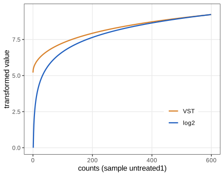
Regularized logarithm (rlog) transformation
The rlog fits, for each gene, the model (8.11) with an intercept and one coefficient per sample, i.e. the \(m\times(m+1)\) design matrix
\[ \X=\begin{pmatrix}1&1&0&0&\cdots\\1&0&1&0&\cdots\\1&0&0&1&\cdots\\\vdots&\vdots&\vdots&\vdots&\ddots\end{pmatrix}, \tag{8.13} \]with a normal prior on the sample coefficients, and returns the fitted \(\log_2q_{ij}=\beta_{i0}+\beta_{ij}\). (The book writes the size as \(K\times(K+1)\) with \(K\) the number of samples; that \(K\) is not the count \(K_{ij}\).)
Filling the gap 8.20: the rlog is a well-posed ridge regression Section 8.10.2, (8.13)
Derivation
Non-identifiability without the prior. \(\X\) in (8.13) has \(m+1\) columns but rank \(m\): the vector \(\mathbf{v}=(1,-1,\dots,-1)^\T\) satisfies \(\X\mathbf{v}=\mathbf{0}\), so adding \(t\) to the intercept and subtracting \(t\) from every sample coefficient leaves all means unchanged and the likelihood has a ridge of maxima.
Uniqueness with the prior. The objective is \(F(\bm b)=-\ell(\X\bm b)+\frac\lambda2\sum_{j\ge1}b_j^2\). The NB log likelihood is strictly concave in the linear predictor \(\bm\eta=\X\bm b\) (its second derivative in each \(\eta_j\) is \(-\mu_j(1+\alpha k_j)/(1+\alpha\mu_j)^2<0\)). Suppose \(\bm b\ne\bm b'\) both minimise \(F\). If \(\X\bm b\ne\X\bm b'\), strict concavity of \(\ell\) in \(\bm\eta\) and convexity of the penalty make the midpoint strictly better. If \(\X\bm b=\X\bm b'\), then \(\bm b-\bm b'=t\mathbf{v}\) with \(t\ne0\), the likelihood is equal along the segment, and the penalty \(\sum_{j\ge1}b_j^2\) is strictly convex along \(\mathbf{v}\) (whose sample components are \(-1\)), so again the midpoint is strictly better. Either way a contradiction: the minimiser is unique.
Shrinkage. For a gene with low counts the likelihood is flat in the sample coefficients, the penalty dominates, and all \(\beta_{ij}\) are pulled to 0: the rlog values of that gene collapse onto its intercept. This is the very low standard deviation of the low-count genes in the right panel of Figure 8.12. For a high-count gene the penalty is negligible and rlog \(\approx\log_2\) of the normalised counts.
Details as implemented. DESeq2 uses the fitted trend \(\alpha_\text{tr}(\bar\mu_i)\) as the dispersion, \(\lambda_0=10^{-6}\) for the intercept, and a prior variance obtained by the same weighted upper-quantile matching as in Filling the gap 8.18, applied to \(\log_2(K_{ij}/s_j+0.5)-\log_2(\bar\mu_i+0.5)\) over all genes and samples (pasilla: 0.0740). The course reproduces this prior variance to \(10^{-16}\) and the rlog values of four genes to \(1.1\times10^{-4}\) (DESeq2 stops its IRLS at a looser tolerance for rlog). ∎
Question 8.12 (mean-sd plots of the three transformations) Section 8.10.2
Answer
Figure 8.12. The leftmost 2,240 genes (the book says about 2,500) have only zero counts and standard deviation 0 under every transformation. For \(\log_2(n+1)\), weakly detected genes have a large standard deviation (the hump, up to about 0.8), exactly as Filling the gap 8.19 predicts. The VST is nearly flat, around 0.15–0.2. The rlog gives very low standard deviations for low-count genes because it shrinks their sample differences to zero (Filling the gap 8.20), and about 0.1 for the rest.
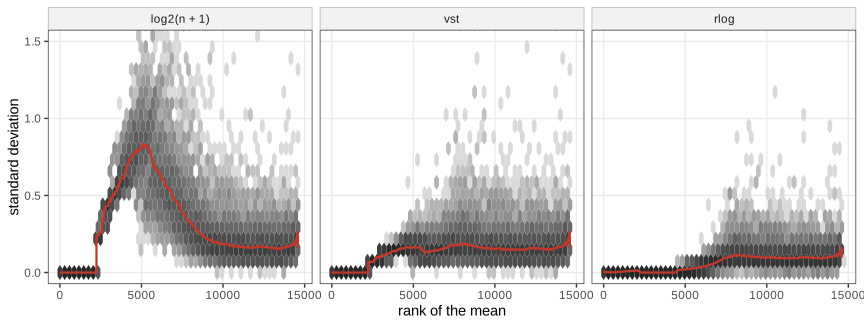
vsn::meanSdPlot). Download: PDF · SVG8.10.3 Dealing with outliers
A single very large count, unrelated to the design, can drive a gene's fold change. DESeq2 computes Cook's distance (Cook 1977) for every count and, by default, sets the p-value of a gene to NA when one of its counts has Cook's distance above the 99% quantile of \(F(p,m-p)\) (pasilla: \(F_{0.99}(2,5)=13.27\), one gene flagged). With 7 or more replicates per group, outlying counts are instead replaced by the trimmed mean of the normalised counts scaled by the sample's size factor, and the gene is refitted.
Filling the gap 8.21: Cook's distance for a GLM Section 8.10.3
Derivation
Definition. Cook's distance of observation \(j\) measures how far the coefficient vector moves when \(j\) is deleted, in the metric of its own covariance: \(D_j=(\hat\bb-\hat\bb_{(-j)})^\T\X^\T\W\X(\hat\bb-\hat\bb_{(-j)})/p\) (natural-log scale, unit dispersion).
One-step formula. Approximate the GLM fit by its last weighted least-squares step, with working residual \(e_j=z_j-\eta_j+o_j=(k_j-\mu_j)/\mu_j\) and weight \(w_j\). Deleting row \(j\) of a weighted least-squares problem changes the solution by (Sherman-Morrison)
\[ \hat{\bm b}-\hat{\bm b}_{(-j)}=\frac{(\X^\T\W\X)^{-1}\mathbf{x}_jw_je_j}{1-h_{jj}},\qquad h_{jj}=w_j\mathbf{x}_j^\T(\X^\T\W\X)^{-1}\mathbf{x}_j, \]where \(h_{jj}\) is the leverage (diagonal of \(\W^{1/2}\X(\X^\T\W\X)^{-1}\X^\T\W^{1/2}\)). Substituting,
\[ D_j=\frac{w_je_j^2}{p}\cdot\frac{h_{jj}}{(1-h_{jj})^2},\qquad w_je_j^2=\frac{\mu_j}{1+\alpha\mu_j}\cdot\frac{(k_j-\mu_j)^2}{\mu_j^2}=\frac{(k_j-\mu_j)^2}{\mu_j+\alpha\mu_j^2}, \]the squared Pearson residual. In DESeq2 the \(\alpha\) in the Pearson residual is a robust method-of-moments estimate rather than the fitted dispersion, so that the outlier cannot inflate its own denominator. The course reproduces DESeq2's hat values and Cook's distances for 50 genes.
Cut-off. In the normal linear model, \(D_j\) equals \(F\)-type statistic for testing \(\bb=\hat\bb_{(-j)}\), so \(D_j>F_{0.99}(p,m-p)\) means that deleting one observation moves the estimate outside the 99% confidence ellipsoid. With few samples \(F_{0.99}(p,m-p)\) is large, so only gross outliers are flagged. ∎
Question 8.13 (controlling the outlier handling) Section 8.10.3
Answer
The cut-off is the cooksCutoff argument of results(): a number replaces the default \(F_{0.99}(p,m-p)\), and cooksCutoff = FALSE switches the filtering off. Replacement of outlying counts is controlled by minReplicatesForReplace in DESeq() (default 7; Inf disables it). The distances are stored as assays(dds)[["cooks"]] (one per count), and their maximum per gene as mcols(dds)$maxCooks.
8.10.4 Tests of log2 fold change above or below a threshold
The lfcThreshold \(\theta\) and altHypothesis arguments of results() turn the point null into an interval null. With \(\beta\) the \(\log_2\) fold change, the four alternatives are greater: \(\beta>\theta\); less: \(\beta<-\theta\); greaterAbs: \(|\beta|>\theta\); lessAbs: \(|\beta|<\theta\). Figure 8.13 shows the genes called at adjusted p < 0.1 for \(\theta=0.5\): 160, 4892, 61 and 78 genes (greaterAbs, lessAbs, greater, less).
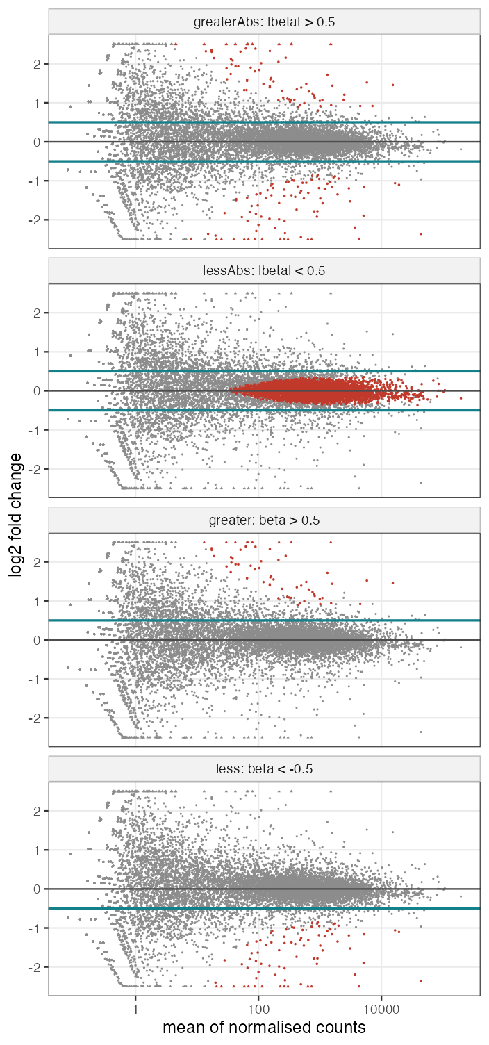
Filling the gap 8.22: p-values for interval null hypotheses Section 8.10.4
Derivation
Treat \(\hat\beta\sim\N(\beta,\mathrm{SE}^2)\) with \(\mathrm{SE}\) known, and let \(b\) be the observed estimate. For a composite null \(H_0\), a valid p-value is \(\sup_{\beta\in H_0}P_\beta(T\) at least as extreme as observed\()\).
greater (\(H_0:\beta\le\theta\)): with \(T=\hat\beta\), \(P_\beta(\hat\beta\ge b)=\bar\Phi((b-\beta)/\mathrm{SE})\) increases in \(\beta\), so the supremum is at \(\beta=\theta\): \(p=\bar\Phi((b-\theta)/\mathrm{SE})\). less is the mirror image, \(p=\Phi((b+\theta)/\mathrm{SE})\).
greaterAbs (\(H_0:|\beta|\le\theta\)): with \(T=|\hat\beta|\), \(P_\beta(|\hat\beta|\ge|b|)=\bar\Phi\big(\frac{|b|-\beta}{\mathrm{SE}}\big)+\Phi\big(\frac{-|b|-\beta}{\mathrm{SE}}\big)\), the tail of a folded normal, which increases in \(|\beta|\) (the distribution of \(|\hat\beta|\) is stochastically increasing in \(|\beta|\)). The supremum is at \(|\beta|=\theta\):
\[ p=\bar\Phi\Big(\frac{|b|-\theta}{\mathrm{SE}}\Big)+\Phi\Big(\frac{-|b|-\theta}{\mathrm{SE}}\Big). \]lessAbs (\(H_0:|\beta|\ge\theta\), i.e. \(\beta\ge\theta\) or \(\beta\le-\theta\)): an intersection-union test. Reject only if both one-sided nulls are rejected; the p-value is \(\max\big(\Phi((b-\theta)/\mathrm{SE}),\ \bar\Phi((b+\theta)/\mathrm{SE})\big)\). Validity: if \(\beta\ge\theta\), rejecting requires rejecting the first one-sided test, whose size is at most the level, and symmetrically. This is the two one-sided tests (TOST) procedure of equivalence testing. These are exactly the p-values of results() (checked to \(10^{-12}\) for all four alternatives). The tests are conservative inside the null region, so they lose power compared with first testing \(\beta=0\) and then filtering on \(|\hat\beta|>\theta\), but unlike that procedure they control the error rate for the interval hypothesis. ∎
Summary
- Read counts are Poisson to excellent approximation within a library (gap 8.1); between biological replicates the rate varies, and a gamma-distributed rate gives the gamma-Poisson law with variance \(\mu+\alpha\mu^2\) (Result 8.1).
- Sequencing depth enters as a size factor per sample, estimated by the median of ratios to the geometric-mean reference: a robust location estimate on the log scale that needs most genes, or balanced changes, to be unchanged (gap 8.3).
- Linear models encode the design in \(\X\); interactions are differences of differences; least squares is normal maximum likelihood, and robust alternatives replace the square by a slower-growing loss solved by reweighted least squares (gap 8.9).
- A GLM combines an exponential-family response, a link and a linear predictor with offset. For the NB model with log link the score is \(\X^\T\W\mathbf{z}^\ast\) and IRLS is Fisher scoring (Algorithm 8.2); Wald and likelihood ratio tests follow from the asymptotics of the MLE (gap 8.13).
- Blocking factors remove nuisance variation and raise power when the design is near balanced (1061 to 1325 discoveries for pasilla; 3386 to 4834 for the paired airway design); confounding biases the estimate by \(\beta_t\delta\) (gap 8.14).
- Dispersions are estimated by the Cox-Reid adjusted likelihood and shrunk towards a trend \(a_0+a_1/\bar\mu\) with a log-normal prior whose width is the observed spread minus the sampling variance \(\psi_1((m-p)/2)\) (Algorithm 8.3). Fold changes can be shrunk by a normal prior: a ridge penalty that shrinks by roughly \(\sigma_\beta^2/(\sigma_\beta^2+\mathrm{SE}^2)\) (gap 8.18).
- For visualisation, the VST \(\frac2{\ln2}\asinh\sqrt{a_0q/(1+a_1)}+\const\) stabilises the standard deviation at \(\sqrt{a_0}/\ln2\) (gap 8.19); the rlog is a ridge regression on per-sample coefficients (gap 8.20).
- Cook's distance flags single influential counts; interval nulls \(|\beta|\le\theta\) test for effects of a relevant size, with p-values taken at the boundary of the null (gap 8.22).
Exercises
The three exercises of Chapter 8 (Holmes and Huber 2019, Section 8.13), restated in my own words, with worked solutions (hidden).
Exercise 8.1 (depletion of small p-values). Simulate 10,000 "genes" with 12 independent standard normal values each, in two versions: \(x_1\) as is, and \(x_2\) in which the six samples of a second batch receive an extra gene-specific shift \(2Z\), \(Z\sim\N(0,1)\). The groups \(a,b\) alternate, so each batch contains three samples of each group, and there is no group effect. With a two-sample \(t\)-test on the group, the p-values are uniform for \(x_1\) but depleted near 0 for \(x_2\) (Figure 8.14). Replace the \(t\)-test by linear models with
~ groupand with~ group + batch, and show that with the batch in the model the p-values of the group coefficient are uniform for both \(x_1\) and \(x_2\).Solution
Simulation (Figure 8.14). The course code computes the gene-wise least-squares fits for all 10,000 genes at once (one matrix product) and the \(t\) p-values of the group coefficient. With
~ groupthe p-values coincide with those of the equal-variance \(t\)-test (genefilter::rowttests, to \(10^{-15}\)): a linear model with one two-level factor is the two-sample \(t\)-test. So for \(x_2\) they are still depleted: only 2.1% are below 0.05. With~ group + batchthey are uniform for \(x_2\) too (5.07% below 0.05; Kolmogorov-Smirnov test does not reject). The book's phrase "uniform in both cases" therefore holds for the model that includes the batch; the model with the group alone reproduces the depletion.Why. Write gene \(i\)'s values as \(x_{ij}=\varepsilon_{ij}+\delta_ib_j\) with \(b_j\) the batch-2 indicator and \(\delta_i=2Z_i\). The batch is balanced within groups, so the group mean difference contains \(\delta_i(\bar b_a-\bar b_b)=0\): the numerator of \(t\) is unaffected. But inside each group \(b_j\) takes the values 0,0,0,1,1,1, so each within-group sample variance contains \(\delta_i^2\cdot\frac{6\cdot(1/2)^2}{5}=0.3\,\delta_i^2\): the pooled variance has expectation \(1+0.3\delta_i^2\) (\(=2.2\) on average). The \(t\)-statistic is divided by an inflated standard error, its null distribution is narrower than \(t_{10}\), and small p-values become rare. With the batch column in \(\X\), the residuals are orthogonal to \(\mathbf{b}\) (Filling the gap 8.7), \(\delta_i\) is absorbed exactly, the residual variance estimates \(\sigma^2=1\) with 9 degrees of freedom, and \(t\sim t_9\) exactly under the null. The same mechanism, seen from the other side, is why blocking increases power (Filling the gap 8.14), and a tilted p-value histogram in a real analysis hints at an unmodelled batch.
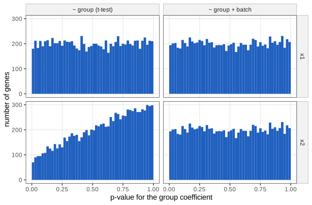
Figure 8.14. P-values of the group coefficient for the simulated \(x_1\) (top) and \(x_2\) (bottom), with the model ~ group(equal to the \(t\)-test, left) and~ group + batch(right). Only the left bottom panel is depleted near 0. The left column reproduces Holmes and Huber (2019), Figure 8.14; the right column is the solution of Exercise 8.1. Download: PDF · SVGExercise 8.2 (edgeR). Repeat the one-factor analysis of Section 8.5 with the edgeR package, compare the p-values with those of DESeq2 in a scatter plot of \(\log_{10}p\), look at the raw counts of genes where the two disagree, and explain the differences.
Solution
Method (function
edger_comparein the course code). Build aDGEList, keep genes passingfilterByExpr(7,919 genes), compute TMM normalisation factors, estimate dispersions withestimateDisp(common, trended and empirical Bayes tagwise dispersions; common dispersion 0.0221), fit the quasi-likelihood GLMglmQLFitwith design~ conditionand test withglmQLFTest.Results. On the same 7,919 genes, edgeR calls 960 genes at FDR 0.1 and DESeq2 1052; 929 are common, 31 are edgeR-only and 123 DESeq2-only. The fold changes agree closely (correlation 0.9986) and the rankings of the p-values agree well (Spearman correlation 0.988 of \(-\log_{10}p\)).
Explanation. (i) The largest differences in \(\log_{10}p\) are at the top of the list: the strongest gene has \(p=4.9\times10^{-165}\) in DESeq2 but \(3.5\times10^{-11}\) in edgeR. The QL test refers its statistic to an \(F(1,d)\) distribution with finite denominator degrees of freedom, whose tail is polynomial, while the Wald test uses the normal tail; this accounts for the uncertainty of the dispersion estimate and makes p-values far more conservative for extreme genes, without changing their rank. (ii) For genes near the threshold, the differences come from the dispersion shrinkage (edgeR's weighted likelihood towards a trend with prior degrees of freedom against DESeq2's log-normal prior, Filling the gap 8.16) and from the normalisation (TMM against the median of ratios). Looking at the raw counts of disagreeing genes typically shows one sample far from its group: one method's dispersion estimate absorbs it and the other's does not.
Exercise 8.3 (robustness). Write an interactive app that fits a regression line to an example data set (for instance
mpgondispinmtcars), lets the user move one point over a wide range, and offers least squares (lm), M-estimation (MASS::rlm) and least trimmed squares or least quantile of squares (MASS::lqs) as fitting methods.Solution
A shiny app needs a slider for the shift of one point, radio buttons for the method, and a plot that refits on each change: the server takes the data, adds the shift to the chosen observation, calls
lm,rlmorlqs(..., method = "lts")and draws the points and the fitted line. The behaviour it shows, computed for the Cadillac Fleetwood (observation 15, displacement 472, a high-leverage point) with itsmpgincreased by \(0,20,40,100\): the least-squares slope moves from \(-0.0412\) through \(-0.0311\) and \(-0.0209\) to \(+0.0095\) (the sign flips), the Huber M-estimate stays at \(-0.0392\) then \(-0.0367\) for every shift (the point's weight falls as \(s/|u|\), Filling the gap 8.9), and LTS stays at \(-0.0334\) once the point is among the discarded residuals. Moving the point in the \(x\) direction instead shows the weakness of M-estimation against leverage points, which LTS resists. We reproducerlmwith a 12-line IRLS.
Demonstrations for this chapter
Each demonstration runs in the browser on the chapter's data (exported by the R code), with seeded random numbers where there is simulation, and links back to these notes. The ▶ Demo boxes above open them already set to the case under discussion.
| Demonstration | What you can see | Sections |
|---|---|---|
| Size factors and the mean-variance relationship | The median of ratios against column sums on the toy example and on pasilla; the variance-mean cloud with Poisson and gamma-Poisson curves; what unbalanced changes do. Presets: 1 toy example (Fig. 8.1); 2 one gene goes wild; 3 pasilla size factors (Fig. 8.2); 4 Poisson versus gamma-Poisson (Fig. 8.3); 5 unbalanced changes. | 8.4.1, 8.4.2, 8.6.1 |
| The negative binomial GLM for one gene | IRLS iterations, the profile log likelihood with its Wald approximation, Wald and likelihood ratio tests, one- and two-factor designs, and fold-change shrinkage. Presets: 1 IRLS for the top gene; 2 adding the blocking factor; 3 shrinkage (Fig. 8.10); 4 a low-count gene; 5 a larger dispersion. | 8.8.3, 8.9, 8.10.1 |
| Dispersion shrinkage and variance stabilisation | Gene-wise Cox-Reid estimates, the trend and the MAP under the log-normal prior, recomputed in the page; the VST against shifted logarithms on simulated replicates. Presets: 1 gene-wise estimates and trend; 2 MAP shrinkage; 3 a narrow prior; 4 VST versus \(\log_2(n+1)\); 5 a larger pseudocount. | 8.10.1, 8.10.2 |
The R code that produces every figure on this page and the demonstration data is code/ch08_count_data_glm.R (see the code index).
References
- Holmes, S. and Huber, W. (2019). Modern Statistics for Modern Biology. Cambridge University Press. Chapter 8.
- Anders, S. and Huber, W. (2010). Differential expression analysis for sequence count data. Genome Biology, 11, R106. doi:10.1186/gb-2010-11-10-r106.
- Anders, S., Reyes, A. and Huber, W. (2012). Detecting differential usage of exons from RNA-seq data. Genome Research, 22(10), 2008–2017. doi:10.1101/gr.133744.111.
- Bourgon, R., Gentleman, R. and Huber, W. (2010). Independent filtering increases detection power for high-throughput experiments. Proceedings of the National Academy of Sciences, 107(21), 9546–9551. doi:10.1073/pnas.0914005107.
- Brooks, A. N., Yang, L., Duff, M. O., et al. (2011). Conservation of an RNA regulatory map between Drosophila and mammals. Genome Research, 21(2), 193–202. doi:10.1101/gr.108662.110.
- Cook, R. D. (1977). Detection of influential observation in linear regression. Technometrics, 19(1), 15–18. doi:10.1080/00401706.1977.10489493.
- Cox, D. R. and Reid, N. (1987). Parameter orthogonality and approximate conditional inference. Journal of the Royal Statistical Society: Series B, 49(1), 1–39. doi:10.1111/j.2517-6161.1987.tb01422.x.
- Himes, B. E., Jiang, X., Wagner, P., et al. (2014). RNA-Seq transcriptome profiling identifies CRISPLD2 as a glucocorticoid responsive gene that modulates cytokine function in airway smooth muscle cells. PLoS ONE, 9(6), e99625. doi:10.1371/journal.pone.0099625.
- Huber, P. J. (1964). Robust estimation of a location parameter. The Annals of Mathematical Statistics, 35(1), 73–101. doi:10.1214/aoms/1177703732.
- Leek, J. T. and Storey, J. D. (2007). Capturing heterogeneity in gene expression studies by surrogate variable analysis. PLoS Genetics, 3(9), e161. doi:10.1371/journal.pgen.0030161.
- Love, M. I., Huber, W. and Anders, S. (2014). Moderated estimation of fold change and dispersion for RNA-seq data with DESeq2. Genome Biology, 15, 550. doi:10.1186/s13059-014-0550-8.
- Nelder, J. A. and Wedderburn, R. W. M. (1972). Generalized linear models. Journal of the Royal Statistical Society: Series A, 135(3), 370–384. doi:10.2307/2344614.
- Robinson, M. D., McCarthy, D. J. and Smyth, G. K. (2010). edgeR: a Bioconductor package for differential expression analysis of digital gene expression data. Bioinformatics, 26(1), 139–140. doi:10.1093/bioinformatics/btp616.
- Rousseeuw, P. J. (1984). Least median of squares regression. Journal of the American Statistical Association, 79(388), 871–880. doi:10.1080/01621459.1984.10477105.
- Rousseeuw, P. J. and Leroy, A. M. (1987). Robust Regression and Outlier Detection. Wiley. doi:10.1002/0471725382.
- Stegle, O., Parts, L., Durbin, R. and Winn, J. (2010). A Bayesian framework to account for complex non-genetic factors in gene expression levels greatly increases power in eQTL studies. PLoS Computational Biology, 6(5), e1000770. doi:10.1371/journal.pcbi.1000770.
- Verhulst, P.-F. (1845). Recherches mathématiques sur la loi d'accroissement de la population. Nouveaux Mémoires de l'Académie Royale des Sciences et Belles-Lettres de Bruxelles, 18, 1–42.
Every number quoted in these notes comes from the course R code, including the comparisons with DESeq2, edgeR and MASS.