Chapter 3. Data visualization
Graphics serve two purposes: to explore data and find out what is in them, and to show others what was found. This chapter of Holmes and Huber (2019) introduces base R plotting and the grammar of graphics implemented in ggplot2, and works through displays of one variable (barplots, boxplots, dot and beeswarm plots, densities, violins, ridgelines, ECDFs), of two (scatterplots, 2-D densities, hexagonal bins, plot shapes), and of more (faceting, colour, heatmaps), ending with transformations, fonts and genome-anchored data. Every graphic computes a statistic before it draws anything; these notes make those statistics explicit and fill in the mathematics behind them.
Ch. 1 Discrete data Ch. 2 Statistical modeling Ch. 3 Data visualization Ch. 4 Mixture models Ch. 5 Clustering Ch. 6 Testing Ch. 7 Multivariate analysis Ch. 8 Count data and GLMs Ch. 9 Heterogeneous data Ch. 10 Networks and trees Ch. 11 Image data Ch. 12 Supervised learning Ch. 13 Experimental design
How to read these notes
They follow the book. Sections carry the book's numbers (3.2, 3.6.4, ...) and its section titles; the book's one displayed equation pair is numbered (3.1), (3.2) as in the book. Figures carry the book's figure numbers.
Filling the gaps. The chapter is about graphics and states little mathematics, but almost every graphic rests on a statistical estimate: a confidence interval behind an error bar, sample quantiles behind a boxplot, a kernel density estimate behind a density, violin or ridgeline plot, the empirical distribution function, local regression behind geom_smooth, binned counts behind a hexagon plot, a change of variables behind a transformed axis. An orange Filling the gap box gives each of these a complete derivation. Derivations start hidden: open one with its bar, or use the button below.
Figures, questions and demonstrations. All figures computed from data are reproduced from scratch by the R code. The book's in-text questions are restated as Question boxes with answers; its end-of-chapter exercises are at the end. The ▶ Demo boxes open an interactive demonstration already set to the case being discussed.
Main reference
S. Holmes and W. Huber, Modern Statistics for Modern Biology, Cambridge University Press (2019), Chapter 3 “Data visualization”. Section, figure, question and exercise numbers below refer to this book. Original papers are listed in the references.
The explanations, derivations and code are my own; results are cited to the book's sections.
The chapter at a glance
- 3.2–3.5 Base R draws on a canvas; ggplot2 builds a plot from data, aesthetic mappings, geometric objects, statistics, scales, coordinates and facets, one layer at a time.
geom_smoothadds a loess fit with a pointwise t band (Gap 3.1). - 3.6 One variable: bars of means with error bars (Gap 3.2), boxplots and sample quantiles (Gap 3.3), kernel density estimates with bias of order \(h^2\), variance of order \(1/(nh)\) and optimal bandwidth of order \(n^{-1/5}\) (Gaps 3.4, 3.5), and the ECDF, which needs no tuning, is unbiased and converges uniformly with a distribution-free band (Gaps 3.6–3.8). Monotone transformations move modes but not quantiles (Gap 3.9).
- 3.7 Two variables: overplotting, transparency, 2-D kernel densities (Gap 3.10), hexagonal binning (Gap 3.11), and the aspect ratio, including banking to 45° (Gap 3.12).
- 3.8–3.10 More dimensions through aesthetics and facets; colour palettes; heatmaps of centred data (Gap 3.13) with dendrogram orderings, of which there are \(2^{n-1}\) (Gap 3.14); the HCL colour space as polar CIELUV (Gap 3.15).
- 3.11–3.13 Variance-stabilising transformations by the delta method (Gap 3.16), the MA plot and why dense regions look more variable (Gap 3.17), plotmath and the volume of the unit ball (Gap 3.18), and genome-anchored plots.
Notation. \(x_1,\dots,x_n\) is a sample from a distribution with cumulative distribution function (CDF) \(F\) and, when it exists, density \(f\); \(x_{(1)}\le\dots\le x_{(n)}\) are the order statistics. \(\mathbf 1\{A\}\) is 1 if \(A\) holds and 0 otherwise. \(\phi\) and \(\Phi\) are the standard normal density and CDF, \(z_p=\Phi^{-1}(p)\). For a function \(g\), \(R(g)=\int g(u)^2\,\d u\). Expression values are log2 intensities unless said otherwise.
Prerequisites. Probability and the normal, binomial and Poisson distributions (Chapters 1 and 2 of the book); Taylor's theorem; the law of large numbers and the central limit theorem.
3.2 Base R plotting
R ships with several graphics systems. The oldest, in the graphics package, works like a pen plotter (Figure 3.1 of the book is a photograph of one, not reproduced here): each call draws onto a canvas, and what has been drawn cannot be moved. The book's first example is the DNase data frame that comes with R: an enzyme-linked immunosorbent assay (ELISA) of deoxyribonuclease activity, with the assay run (Run), the protein concentration (conc, ng/ml) and the measured optical density (density), 176 rows from 11 runs (Holmes and Huber 2019, Section 3.2).
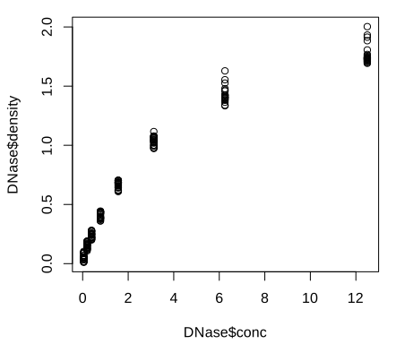
plot() and its defaults: open circles and the column expressions as axis labels. Code: fig_3_2. Reproduces Holmes and Huber (2019), Figure 3.2. PDF · SVGArguments change the plot symbol (pch), colour and labels; the labels can come from attributes stored with the data frame (attr(DNase, "labels"), attr(DNase, "units")).
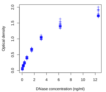
pch = 3, blue) and axis labels taken from the metadata stored with the data set. Code: fig_3_3. Reproduces Holmes and Huber (2019), Figure 3.3. PDF · SVGhist() and boxplot() give the distribution of the densities, overall and per run.
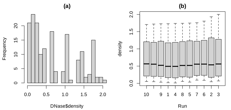
Run (10, 11, 9, 1, ...), which is fixed by the data set, not alphabetical (see the note in Section 3.2). Code: fig_3_4. Reproduces Holmes and Huber (2019), Figure 3.4. PDF · SVGNote on Figure 3.4(b): the order of the boxes
The book's caption says the boxes are in lexicographic order because the runs are stored as text. They are not: DNase$Run is an ordered factor (the data set is a grouped-data object from the nlme package), with levels 10 < 11 < 9 < 1 < 4 < 8 < 5 < 7 < 6 < 2 < 3, sorted by each run's largest response. boxplot uses the level order. Lexicographic order would be 1, 10, 11, 2, .... (Verified in R.)
Question 3.1 (column metadata)
Storing descriptions and units with the columns of a data frame is useful. Is the DNase way (attributes) a standard? What else is there?
Answer
Attributes on a data.frame are not a convention that functions respect: most operations (subsetting, merge, dplyr verbs) drop them. Bioconductor's S4Vectors::DataFrame carries a metadata table about its columns (mcols()), and SummarizedExperiment uses DataFrames to annotate both the rows (features) and the columns (samples) of an assay matrix; this is the standard way in Bioconductor.
3.3 An example dataset
Most of the chapter uses the Hiiragi2013 data (Ohnishi et al. 2014): Affymetrix mouse 430 2.0 arrays of single cells from mouse embryos at embryonic days E3.25, E3.5 and E4.5, normalised by RMA (Irizarry et al. 2003) and stored as an ExpressionSet x with 45,101 probes (rows) and 101 cells (columns). The book's Figure 3.5, an immunofluorescence image of a blastocyst, is a micrograph and is not reproduced. Around E3.5 wild-type cells separate into epiblast (EPI) and primitive endoderm (PE); in embryos with the gene Fgf4 knocked out (FGF4-KO) this separation fails. The authors grouped the cells into 8 groups with a colour each (Holmes and Huber 2019, Section 3.3):
| sample group | E3.25 | E3.25 (FGF4-KO) | E3.5 (EPI) | E3.5 (FGF4-KO) | E3.5 (PE) | E4.5 (EPI) | E4.5 (FGF4-KO) | E4.5 (PE) |
|---|---|---|---|---|---|---|---|---|
| cells | 36 | 17 | 11 | 8 | 11 | 4 | 10 | 4 |
The table is made with dplyr: group_by(pData(x), sampleGroup) |> summarise(n = n(), color = unique(sampleColour)). The pipe a |> f(b) means f(a, b), so a chain of pipes reads in the order the operations happen; group_by marks the groups and summarise computes one row per group.
3.4 ggplot2
ggplot2 (Wickham 2016) implements Wilkinson's (2005) grammar of graphics. The plot of Figure 3.2 becomes a short “sentence”: a data frame, an aesthetic mapping (which column goes to which visual property) and a geometric object.
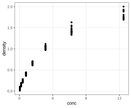
DNase, aesthetics conc and density, geometric object geom_point. Code: fig_3_6. Reproduces Holmes and Huber (2019), Figure 3.6. PDF · SVGFor the group sizes, geom_bar(stat = "identity") draws one bar per row with the height taken from n; the default stat = "count" would instead count rows per x value, which here would give 8 bars of height 1.
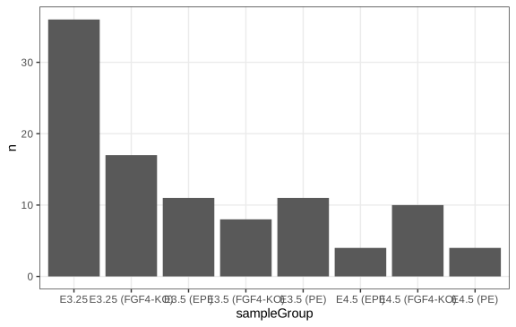
geom_bar(stat = "identity"): the bar heights are the counts in the table groups, not counts computed by ggplot2. Code: fig_3_7. Reproduces Holmes and Huber (2019), Figure 3.7. PDF · SVG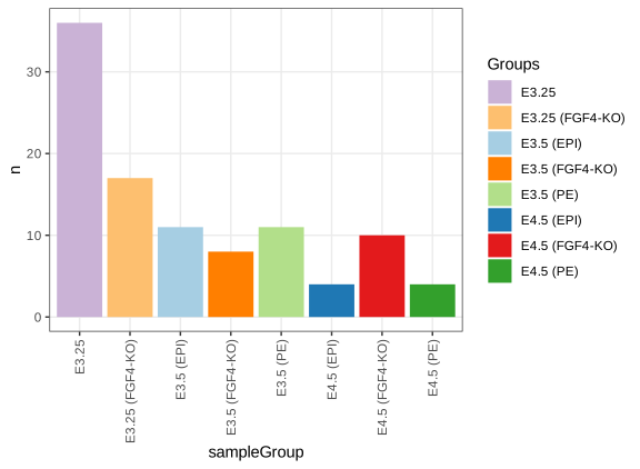
scale_fill_manual) and with rotated, readable labels. Code: fig_3_8. Reproduces Holmes and Huber (2019), Figure 3.8. PDF · SVGTask (horizontal bars)
Swap the aesthetics to get horizontal bars: ggplot(groups, aes(x = n, y = sampleGroup, fill = sampleGroup)) + geom_col() (geom_col is geom_bar(stat = "identity")). Long group names are then readable without rotation, which is a good reason to prefer horizontal bars for categorical labels.
3.4.1 Data flow
ggplot expects a data frame in which each row is one observation and each mapped variable a column. The call returns an object; nothing is drawn until the object is printed, explicitly (print(gg)) or by auto-printing at the console. This is why plots inside loops or sourced scripts need print, and why a plot can be stored, modified with + and drawn later.
3.4.2 Saving figures
ggsave writes a plot to a file. Vector formats (PDF, SVG) store drawing instructions and can be scaled without loss; raster formats (PNG) store pixels: a figure \(w\) inches wide at \(r\) dots per inch has \(wr\) pixel columns, and enlarging it beyond that shows the pixels. Vector files of plots with tens of thousands of points become large and slow, which is why the dense figures of this page (Figures 3.27, 3.28, 3.30, 3.31, 3.41, 3.43) are shown as PNG.
3.5 The grammar of graphics
Definition 3.1 (the components of a ggplot2 graphic) Section 3.5
A graphic is specified by (i) one or more data sets; (ii) one or more geometric objects (points, lines, bars, polygons, ...) that represent the data; (iii) aesthetic mappings from variables to visual properties (position, colour, size, shape, transparency), each with a scale (linear, logarithmic, discrete, ...); (iv) a coordinate system; (v) statistical transformations (identity, counting, binning, smoothing, density estimation) applied before drawing; (vi) a facet specification that splits the data into panels; (vii) theme settings for non-data elements. Items (i)–(iii) are required; the others have defaults (Cartesian coordinates, the identity statistic of most geoms, a single panel, the default theme). Several layers, each a geom with its statistic, can be stacked.
In Figures 3.7 and 3.8 the data are groups (the book calls them “groupsize” at this point), the group names are mapped to x on a discrete scale and the counts to y on a linear scale. Figure 3.9 has three layers from two geoms: points, and from geom_smooth a fitted curve with a band. The data frame dftx holds the transposed expression matrix (cells in rows, 45,101 probe columns with names such as X1426642_at) next to the cell annotation.
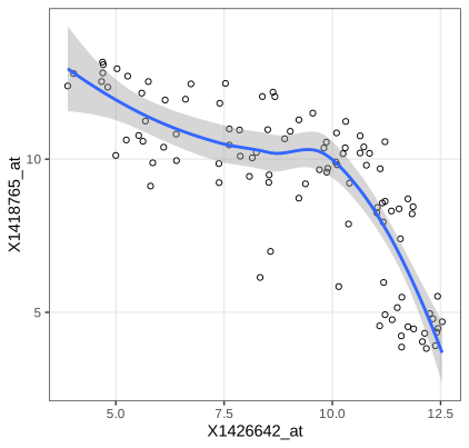
geom_smooth; see Filling the gap 3.1 for what the band means). Code: fig_3_9. Reproduces Holmes and Huber (2019), Figure 3.9. PDF · SVGAlgorithm 3.1 (loess, as used by geom_smooth(method = "loess")) Section 3.5, Figure 3.9
Input: pairs \((x_i,y_i)\), \(i=1,\dots,n\); span \(\alpha=0.75\); degree 2. For each point \(x_0\) where the curve is wanted:
- Let \(q=\lfloor\alpha n\rfloor\) and \(d(x_0)\) the \(q\)-th smallest of the distances \(|x_i-x_0|\).
- Give observation \(i\) the tricube weight \(w_i=T(|x_i-x_0|/d(x_0))\), \(T(u)=(1-u^3)^3\) for \(0\le u<1\) and 0 otherwise.
- Fit \(y\approx\beta_0+\beta_1(x-x_0)+\beta_2(x-x_0)^2\) by weighted least squares and return \(\hat y(x_0)=\hat\beta_0\).
ggplot2 evaluates this on 80 points across the data range and draws the band \(\hat y(x_0)\pm t_{0.975,\nu}\,\hat\sigma\,\|\boldsymbol\ell(x_0)\|\) explained below. The "gaussian" family is used, i.e. no robustness iterations (Cleveland 1979; Cleveland and Devlin 1988).
Filling the gap 3.1: loess is a linear smoother, and what its band means Section 3.5, Figures 3.9, 3.10
The book draws the curve and the grey band without saying what they estimate. Assume \(y_i=m(x_i)+\varepsilon_i\) with independent errors of mean 0 and variance \(\sigma^2\).
Derivation
Linearity. Let \(\mathbf X_0\) be the \(n\times3\) matrix with rows \((1,\,x_i-x_0,\,(x_i-x_0)^2)\) and \(\mathbf W_0=\diag(w_1,\dots,w_n)\). Weighted least squares minimises \((\mathbf y-\mathbf X_0\bm\beta)^\T\mathbf W_0(\mathbf y-\mathbf X_0\bm\beta)\); the normal equations \(\mathbf X_0^\T\mathbf W_0\mathbf X_0\bm\beta=\mathbf X_0^\T\mathbf W_0\mathbf y\) give, when \(\mathbf X_0^\T\mathbf W_0\mathbf X_0\) is invertible (at least three distinct \(x_i\) with positive weight),
\[ \hat y(x_0)=\mathbf e_1^\T(\mathbf X_0^\T\mathbf W_0\mathbf X_0)^{-1}\mathbf X_0^\T\mathbf W_0\,\mathbf y=\boldsymbol\ell(x_0)^\T\mathbf y . \]The weights depend only on the \(x_i\), so \(\hat y(x_0)\) is a fixed linear combination of the responses (the “equivalent kernel” \(\boldsymbol\ell(x_0)\)). Stacking the rows \(\boldsymbol\ell(x_i)^\T\) gives the smoother matrix \(\mathbf L\), \(\hat{\mathbf y}=\mathbf L\mathbf y\).
Variance. \(\var\hat y(x_0)=\boldsymbol\ell(x_0)^\T(\sigma^2\mathbf I)\boldsymbol\ell(x_0)=\sigma^2\|\boldsymbol\ell(x_0)\|^2\).
Estimating \(\sigma^2\). The residuals are \((\mathbf I-\mathbf L)\mathbf y\), so \(\mathrm{RSS}=\mathbf y^\T\mathbf A\mathbf y\) with \(\mathbf A=(\mathbf I-\mathbf L)^\T(\mathbf I-\mathbf L)\). For any symmetric \(\mathbf A\), \(\E[\bm\varepsilon^\T\mathbf A\bm\varepsilon]=\sum_{ij}A_{ij}\E[\varepsilon_i\varepsilon_j]=\sigma^2\Tr\mathbf A\). If the smoother reproduces \(m\) (no bias, \((\mathbf I-\mathbf L)\mathbf m=\mathbf 0\)), then \(\E\,\mathrm{RSS}=\sigma^2\delta_1\) with
\[ \delta_1=\Tr\{(\mathbf I-\mathbf L)^\T(\mathbf I-\mathbf L)\}=n-2\Tr\mathbf L+\Tr(\mathbf L^\T\mathbf L), \]so \(\hat\sigma^2=\mathrm{RSS}/\delta_1\) is unbiased. For ordinary least squares \(\mathbf L\) is a projection of rank \(p\) and \(\delta_1=n-p\), the usual degrees of freedom. R's loess uses this \(\hat\sigma\) and the “lookup” degrees of freedom \(\nu=\delta_1^2/\delta_2\), \(\delta_2=\Tr(\mathbf A^2)\), which matches the first two moments of \(\mathrm{RSS}/\sigma^2\) to a scaled \(\chi^2_\nu\) (under normal errors \(\mathrm{RSS}/\sigma^2\) is a weighted sum of \(\chi^2_1\) variables with weights the eigenvalues of \(\mathbf A\); a scaled \(\chi^2_\nu\) with the same mean and variance has \(\nu=(\sum\lambda)^2/\sum\lambda^2\)).
The band. Under normal errors \((\hat y(x_0)-\E\hat y(x_0))/(\hat\sigma\|\boldsymbol\ell(x_0)\|)\) is approximately \(t_\nu\), so \(\hat y(x_0)\pm t_{0.975,\nu}\hat\sigma\|\boldsymbol\ell(x_0)\|\) covers \(\E\hat y(x_0)\) with probability about 0.95 at each \(x_0\) separately. Two caveats: it is a band for the smoothed curve \(\E\hat y(x_0)=\boldsymbol\ell(x_0)^\T\mathbf m\), not for \(m(x_0)\) (the smoothing bias is not in it), and it is pointwise, not simultaneous. In Figure 3.10 the errors are also clearly not identically distributed across groups.
We reproduce predict(loess(...)) at several \(x_0\) from the weighted least-squares formula, \(\hat\sigma\) from \(\mathrm{RSS}/\delta_1\) and the standard errors from \(\hat\sigma\|\boldsymbol\ell(x_0)\|\), to \(10^{-8}\) (exact computation, surface = "direct"; the default interpolates the fit from a k-d tree, which changes the values slightly). ∎
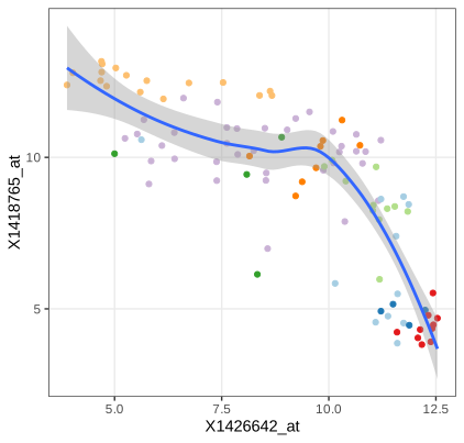
fig_3_10. Reproduces Holmes and Huber (2019), Figure 3.10. PDF · SVGQuestion 3.2 (colour in all layers)
In Figure 3.10 the colour mapping is given only to geom_point. What happens if it is moved into ggplot(aes(...)), so that every layer inherits it?
Answer
A mapping to a discrete variable also defines groups. geom_smooth then fits one loess curve per sample group, eight curves with eight bands. Several groups have only 4 to 11 cells, too few for a degree-2 loess with span 0.75 to be stable, so expect warnings, erratic curves or missing groups. Mappings in ggplot() are defaults for all layers; mappings in a layer apply to that layer only.
Question 3.3 (is a fitted line always meaningful?)
Should a scatterplot always get a regression line, as in Figures 3.9 and 3.10?
Answer
No. A curve of \(y\) on \(x\) estimates \(\E[y\mid x]\); it suits a response-and-predictor situation. Here the two genes play symmetric roles, and the regression of \(x\) on \(y\) would be a different curve (for a bivariate normal the two lines have slopes \(\rho\sigma_y/\sigma_x\) and \(\sigma_y/(\rho\sigma_x)\), equal only if \(|\rho|=1\)). The cells also form groups with different relationships (Figure 3.10), so one curve through all of them averages over a mixture and can show a trend that no group has. And the band of Gap 3.1 assumes independent errors with constant variance, which the PE cells violate.
The probes are 1426642_at (gene Fn1, fibronectin 1) and 1418765_at (Timd2), found with AnnotationDbi::select(mouse4302.db, ...). Many geoms come with a default statistic: geom_histogram bins the data before drawing bars.
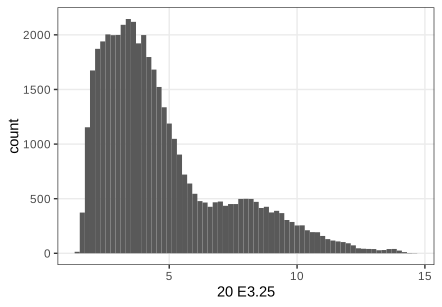
geom_histogram bins the data by itself (statistic bin). Code: fig_3_11. Reproduces Holmes and Huber (2019), Figure 3.11. PDF · SVGQuestion 3.4 (dfx and dftx)
What is the difference between dfx and dftx, and why are both needed?
Answer
dfx is the expression matrix as a data frame: 45,101 rows (probes) by 101 columns (cells), so a plot of one cell's intensities across probes (Figure 3.11) or of one cell against another (Figure 3.27) maps columns of dfx. dftx is the transpose with the cell annotation attached: 101 rows (cells) by 45,101 + 11 columns, so a plot of one gene against another across cells, coloured by cell group (Figure 3.10), maps columns of dftx. ggplot2 maps columns, so the orientation must match what each point represents.
A plot object can be built up step by step. Without a geom it shows only the axes; layers, aesthetics, themes and scales are then added with +, and a different coordinate system turns the bars into wedges.
fig_3_12. Reproduces Holmes and Huber (2019), Figure 3.12. PDF · SVG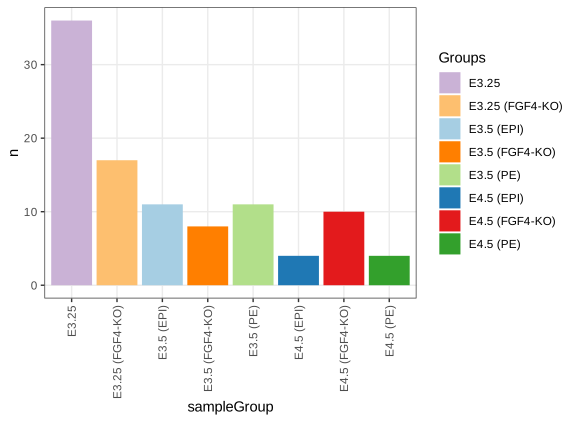
pb after adding a bar layer, a fill aesthetic, a theme change and a fill scale with +. Code: fig_3_13. Reproduces Holmes and Huber (2019), Figure 3.13. PDF · SVG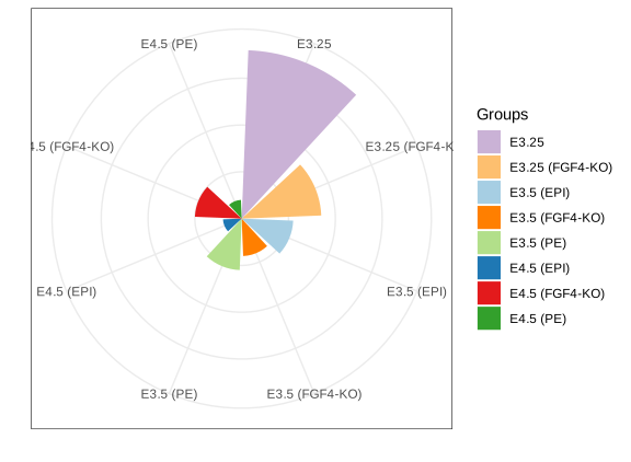
coord_polar()): bar length becomes radius, which exaggerates large values because area grows with the square of the radius. Code: fig_3_14. Reproduces Holmes and Huber (2019), Figure 3.14. PDF · SVG3.6 Visualizing data in 1D
The comparisons of this section use four genes measured in all 101 cells: Fgf4 (probe 1420085_at), Gata4 (1418863_at), Gata6 (1425463_at) and Sox2 (1416967_at), reshaped with reshape2::melt into a long data frame genes with one row per gene and cell (404 rows) (Holmes and Huber 2019, Section 3.6).
3.6.1 Barplots
A bar of height equal to the mean is a common display, but it reduces 101 values to one number and fills a large area with ink that carries no information. If the mean is a poor summary (skewed, multimodal, outliers) the picture misleads.
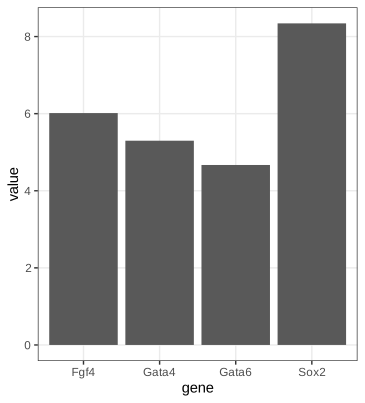
fig_3_15. Reproduces Holmes and Huber (2019), Figure 3.15. PDF · SVG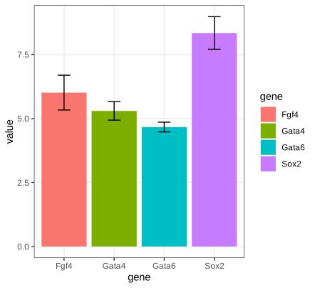
mean_cl_normal. These are 95% t confidence intervals for the mean, about two standard errors either way, not one standard error (Filling the gap 3.2). Code: fig_3_16. Reproduces Holmes and Huber (2019), Figure 3.16. PDF · SVGFilling the gap 3.2: the error bars are 95% t intervals, not standard errors Section 3.6.1, Figure 3.16
The book's caption and text say the error bars show the standard error of the mean. Hmisc::smean.cl.normal, which mean_cl_normal calls, returns \(\bar x\pm t_{0.975,n-1}\,s/\sqrt n\) with \(s\) the sample standard deviation: a 95% confidence interval. With \(n=101\), \(t_{0.975,100}=1.984\), so the bars are almost twice as long as one standard error. (Checked to \(10^{-12}\) for the four genes.)
Result 3.1 (the t interval)
If \(X_1,\dots,X_n\) are independent \(\N(\mu,\sigma^2)\), \(n\ge2\), then \(T=\sqrt n(\bar X-\mu)/S\sim t_{n-1}\), and \(\bar X\pm t_{1-\alpha/2,n-1}S/\sqrt n\) contains \(\mu\) with probability exactly \(1-\alpha\).
Proof, and what one standard error covers
\(\bar X\sim\N(\mu,\sigma^2/n)\), so \(Z=\sqrt n(\bar X-\mu)/\sigma\sim\N(0,1)\). Write \(\mathbf X=\mu\mathbf 1+\sigma\mathbf Z\) with \(\mathbf Z\) standard normal in \(\R^n\) and let \(\mathbf Q\) be an orthogonal matrix whose first row is \(\mathbf 1^\T/\sqrt n\). Then \(\mathbf Y=\mathbf Q\mathbf Z\) is again standard normal, \(Y_1=\sqrt n\bar Z\), and \(\sum_i(Z_i-\bar Z)^2=\|\mathbf Z\|^2-n\bar Z^2=\|\mathbf Y\|^2-Y_1^2=\sum_{i\ge2}Y_i^2\). Hence \((n-1)S^2/\sigma^2=\sum_{i\ge2}Y_i^2\sim\chi^2_{n-1}\) and it is independent of \(Y_1\), i.e. of \(\bar X\). By definition of Student's distribution, \(T=Z/\sqrt{\chi^2_{n-1}/(n-1)}\sim t_{n-1}\), and \(\Pr(|T|\le t_{1-\alpha/2,n-1})=1-\alpha\) rearranges to the interval.
Error bars of \(\pm S/\sqrt n\) correspond to \(|T|\le1\), with coverage \(2F_{t_{n-1}}(1)-1\): 0.657 for \(n=10\) (a simulation gives 0.656) and about 0.68 for large \(n\). Two such bars that just fail to overlap therefore say much less than two 95% intervals that fail to overlap. Without normality, the central limit theorem and Slutsky's lemma give \(T\to\N(0,1)\) in distribution, so the interval is asymptotically valid; for skewed data and small \(n\) its coverage can be poor. ∎
3.6.2 Boxplots
Definition 3.2 (quantile function and sample quantiles)
The quantile function of a CDF \(F\) is \(Q(p)=\inf\{x:F(x)\ge p\}\), \(0<p<1\). R's default sample quantile (type 7, used by ggplot2's boxplots) interpolates the order statistics: with \(h=(n-1)p+1\),
\[ \hat Q(p)=x_{(\lfloor h\rfloor)}+(h-\lfloor h\rfloor)\,\bigl(x_{(\lfloor h\rfloor+1)}-x_{(\lfloor h\rfloor)}\bigr). \]The interquartile range is \(\operatorname{IQR}=\hat Q(0.75)-\hat Q(0.25)\).
Definition 3.3 (Tukey's boxplot, as drawn by geom_boxplot)
A box from \(\hat Q(0.25)\) to \(\hat Q(0.75)\) with a line at the median; whiskers to the most extreme observations within \(1.5\,\operatorname{IQR}\) of the box; observations beyond the whiskers drawn individually. (Base R's boxplot uses Tukey's hinges from fivenum, which can differ slightly from type-7 quartiles.)
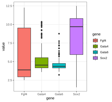
fig_3_17. Reproduces Holmes and Huber (2019), Figure 3.17. PDF · SVGGata4 and Gata6 are concentrated with a few high values; the median of Fgf4 sits near the bottom of its box (right skew) and that of Sox2 near the top (left skew). The boxplots cannot show that Fgf4 and Sox2 are bimodal (Figure 3.19).
Filling the gap 3.3: how many “outliers” to expect, and how precise a quantile is Section 3.6.2
(a) For normal data a point beyond the whiskers is not rare evidence of anything: the population fences \(Q(1/4)-1.5\,\mathrm{IQR}\) and \(Q(3/4)+1.5\,\mathrm{IQR}\) sit at \(\mu\pm2.698\sigma\), and each point falls outside with probability \(2\Phi(-4z_{0.75})=0.0070\). (b) The sample quantile \(\hat Q(p)\) is asymptotically normal with variance \(p(1-p)/(nf(Q(p))^2)\), so quantiles in sparse regions (small \(f\)) are imprecise.
Derivation
(a) For \(\N(\mu,\sigma^2)\), \(Q(3/4)=\mu+z_{0.75}\sigma\) with \(z_{0.75}=0.6745\), so \(\mathrm{IQR}=2z_{0.75}\sigma=1.349\sigma\) and the upper fence is \(\mu+(z_{0.75}+3z_{0.75})\sigma=\mu+4z_{0.75}\sigma=\mu+2.698\sigma\). By symmetry the probability of falling outside either fence is \(2\Phi(-2.698)=0.00698\). In a sample of 101 normal values about 0.7 points are expected beyond the whiskers (more, since the sample quartiles are themselves noisy).
(b) Let \(\xi=Q(p)\), assume \(f\) is continuous and positive at \(\xi\), and use the inverse-ECDF quantile \(\hat Q_n(p)=\inf\{x:F_n(x)\ge p\}\) (type 7 differs from it by at most one spacing, \(O_P(1/n)\), which does not affect the \(\sqrt n\) limit). For fixed \(t\) let \(x_n=\xi+t/\sqrt n\). Because \(\hat Q_n(p)\le x\iff F_n(x)\ge p\) (the Galois inequality of Gap 3.8 applied to \(F_n\)),
\[ \Pr\bigl(\sqrt n(\hat Q_n(p)-\xi)\le t\bigr)=\Pr\bigl(F_n(x_n)\ge p\bigr). \]\(nF_n(x_n)\sim\mathrm{Bin}(n,p_n)\) with \(p_n=F(x_n)=p+f(\xi)t/\sqrt n+o(n^{-1/2})\). Standardising,
\[ \Pr\bigl(F_n(x_n)\ge p\bigr)=\Pr\Bigl(\frac{\sqrt n(F_n(x_n)-p_n)}{\sqrt{p_n(1-p_n)}}\ge-\frac{\sqrt n(p_n-p)}{\sqrt{p_n(1-p_n)}}\Bigr)\to\Pr\Bigl(Z\ge-\frac{f(\xi)t}{\sqrt{p(1-p)}}\Bigr)=\Phi\Bigl(\frac{f(\xi)t}{\sqrt{p(1-p)}}\Bigr), \]using the central limit theorem for the binomial triangular array (Lindeberg's condition holds for bounded summands, or use the Berry–Esseen bound) and \(p_n\to p\). The right side is the CDF of \(\N(0,p(1-p)/f(\xi)^2)\) at \(t\). For the median of Exp(1) with \(n=400\) this predicts variance \(0.25/(400\cdot0.25)=0.0025\); a simulation gives 0.00247. A sharper statement is Bahadur's (1966) representation \(\hat Q_n(p)=\xi+(p-F_n(\xi))/f(\xi)+o_P(n^{-1/2})\). ∎
3.6.3 Dot plots and beeswarm plots
With a hundred points per group it is better to show the points themselves. Overlap is avoided by moving points sideways: the dot plot bins the values (here to width 1/6) and stacks each bin, the beeswarm keeps exact values and shifts a point sideways only when it would overlap one already placed (Wilkinson 1999; package ggbeeswarm). The sideways position carries no information; it is a layout device.
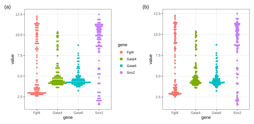
fig_3_18. Reproduces Holmes and Huber (2019), Figure 3.18. PDF · SVG3.6.4 Density plots
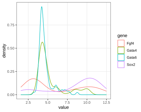
fig_3_19. Reproduces Holmes and Huber (2019), Figure 3.19. PDF · SVGSmoothing the data into a density estimate shows what the boxplots hid: Fgf4 and Sox2 are bimodal, Gata4 and Gata6 have a baseline with a long tail of higher values. The price is a smoothing parameter, and a curve that no longer shows how many observations it rests on (Holmes and Huber 2019, Section 3.6.4).
Definition 3.4 (kernel density estimate)
Let \(K\) be a probability density symmetric about 0 with \(\int u^2K(u)\,\d u=1\), and \(h>0\). The kernel density estimate (Rosenblatt 1956; Parzen 1962) is
\[ \hat f_h(x)=\frac1n\sum_{i=1}^nK_h(x-x_i),\qquad K_h(u)=\frac1hK\Bigl(\frac uh\Bigr). \]With this normalisation \(h\) is the standard deviation of the kernel, the convention of R's density(bw = ...). geom_density uses the Gaussian kernel \(K=\phi\) and Silverman's rule bw.nrd0, \(h=0.9\min(s,\operatorname{IQR}/1.34)\,n^{-1/5}\).
\(\hat f_h\) is a density: it is nonnegative and \(\int\hat f_h=\frac1n\sum_i\int K_h(x-x_i)\,\d x=1\).
Filling the gap 3.4: bias and variance of a kernel density estimate Section 3.6.4
The book says that a small window gives “wiggly” estimates and a large one smooths peaks away. Quantitatively, for fixed \(x\):
Result 3.2 (pointwise bias and variance)
Let \(X_1,\dots,X_n\) be independent with density \(f\), twice continuously differentiable and bounded with bounded \(f''\), and \(K\) as in Definition 3.4 with \(R(K)=\int K^2<\infty\). As \(h\to0\),
\[ \E\hat f_h(x)-f(x)=\tfrac12h^2f''(x)+o(h^2),\qquad \var\hat f_h(x)=\frac{R(K)f(x)}{nh}+O\Bigl(\frac1n\Bigr). \]Hence \(\hat f_h(x)\to f(x)\) in mean square if \(h\to0\) and \(nh\to\infty\).
Proof
Mean. The summands are identically distributed, so \(\E\hat f_h(x)=\E K_h(x-X)=\int\frac1hK\bigl(\frac{x-y}h\bigr)f(y)\,\d y=\int K(u)f(x-hu)\,\d u\) (substitute \(y=x-hu\)). Taylor's theorem with remainder: \(f(x-hu)=f(x)-huf'(x)+\tfrac12h^2u^2f''(x-\theta hu)\) for some \(\theta\in(0,1)\). Integrate against \(K\): \(\int K=1\), \(\int uK=0\) by symmetry, and \(\int u^2K(u)f''(x-\theta hu)\,\d u\to f''(x)\int u^2K=f''(x)\) by dominated convergence (\(f''\) bounded and continuous). So the bias is \(\tfrac12h^2f''(x)+o(h^2)\).
Variance. By independence \(\var\hat f_h(x)=\frac1n\var K_h(x-X)=\frac1n\bigl\{\E K_h(x-X)^2-(\E K_h(x-X))^2\bigr\}\). The same substitution gives \(\E K_h(x-X)^2=\frac1h\int K(u)^2f(x-hu)\,\d u=\frac1h\{R(K)f(x)+o(1)\}\), while \((\E K_h)^2=f(x)^2+o(1)=O(1)\). Hence \(\var\hat f_h(x)=R(K)f(x)/(nh)+o(1/(nh))+O(1/n)\). ∎
Reading the result. At a peak \(f''<0\), so the estimate is biased down; in a trough \(f''>0\) and it is biased up: smoothing flattens peaks and fills valleys, and a large \(h\) can merge two modes into one. The variance grows like \(1/(nh)\): the effective number of observations in a window of width \(h\) is about \(nhf(x)\). Both formulas are checked in R for a normal truth, where \(\E\hat f_h(x)\) is exactly the \(\N(0,1+h^2)\) density, so the bias is \(\phi_{\sqrt{1+h^2}}(x)-\phi(x)\) and its difference from \(\tfrac12h^2f''(x)\) is \(O(h^4)\).
Filling the gap 3.5: the optimal bandwidth, the normal reference rules, and the kernel Section 3.6.4
Integrating the pointwise mean squared error of Result 3.2 over \(x\) gives the asymptotic mean integrated squared error
\[ \operatorname{AMISE}(h)=\tfrac14h^4R(f'')+\frac{R(K)}{nh}. \]Result 3.3 (AMISE-optimal bandwidth)
\(\operatorname{AMISE}\) is minimised by \(h^*=\bigl(R(K)/(R(f'')\,n)\bigr)^{1/5}\), with minimum \(\tfrac54R(K)^{4/5}R(f'')^{1/5}n^{-4/5}\). For \(f=\N(\mu,\sigma^2)\) and a Gaussian kernel, \(h^*=(4/3)^{1/5}\sigma n^{-1/5}=1.059\,\sigma n^{-1/5}\).
Derivation
\(\frac{\d}{\d h}\operatorname{AMISE}=h^3R(f'')-R(K)/(nh^2)\), which is negative for small \(h\), positive for large \(h\) and zero only at \(h^5=R(K)/(R(f'')n)\); the second derivative \(3h^2R(f'')+2R(K)/(nh^3)\) is positive, so this is the minimum. Substituting, both terms are proportional to \(n^{-4/5}\): \(\tfrac14h^{*4}R(f'')=\tfrac14R(K)^{4/5}R(f'')^{1/5}n^{-4/5}\) and \(R(K)/(nh^*)=R(K)^{4/5}R(f'')^{1/5}n^{-4/5}\), total \(\tfrac54(\cdot)\). The error decreases like \(n^{-4/5}\), slower than the \(n^{-1}\) of a parametric estimate: the price of not assuming a shape.
Normal reference. For \(f(x)=\sigma^{-1}\phi(z)\), \(z=(x-\mu)/\sigma\): \(f''(x)=\sigma^{-3}(z^2-1)\phi(z)\), so \(R(f'')=\sigma^{-5}\int(z^2-1)^2\phi(z)^2\,\d z\). Now \(\phi(z)^2=\frac1{2\pi}e^{-z^2}=\frac1{2\sqrt\pi}\cdot\phi_{1/\sqrt2}(z)\), the \(\N(0,\tfrac12)\) density times \(1/(2\sqrt\pi)\). For \(W\sim\N(0,\tfrac12)\), \(\E(W^2-1)^2=\E W^4-2\E W^2+1=\tfrac34-1+1=\tfrac34\). So \(R(f'')=3/(8\sqrt\pi\sigma^5)\). With \(R(\phi)=1/(2\sqrt\pi)\), \(h^{*5}=\frac{1/(2\sqrt\pi)}{3n/(8\sqrt\pi\sigma^5)}=\frac{4\sigma^5}{3n}\).
The rules in R. Replacing \(\sigma\) by the robust \(\hat\sigma=\min(s,\operatorname{IQR}/1.34)\) (the IQR of a normal is \(1.349\sigma\)) gives Scott's rule bw.nrd, \(1.06\hat\sigma n^{-1/5}\). Silverman (1986) lowered the constant to 0.9 (bw.nrd0, ggplot2's default) because the normal reference oversmooths skewed and multimodal densities, which have a larger \(R(f'')\) than the normal with the same spread. For the bimodal Fgf4, \(\hat\sigma=s\) and bw.nrd0 = 1.234. Plug-in rules that estimate \(R(f'')\) from the data (Sheather and Jones 1991, bw.SJ) usually choose smaller bandwidths for such data.
Exact MISE for a normal truth. We also verify the closed form, for \(f=\N(0,1)\) and a Gaussian kernel,
\[ \operatorname{MISE}(h)=\frac1{2\sqrt\pi}\Bigl\{\frac1{nh}+\frac{1-1/n}{\sqrt{1+h^2}}-\frac{2\sqrt2}{\sqrt{2+h^2}}+1\Bigr\}, \]which follows from \(\operatorname{MISE}=\int\E\hat f^2-2\int f\E\hat f+\int f^2\) and the identity \(\int\phi_a(x-\mu_1)\phi_b(x-\mu_2)\,\d x=\phi_{\sqrt{a^2+b^2}}(\mu_1-\mu_2)\): \(\int f^2=\phi_{\sqrt2}(0)\), \(\int f\,\E\hat f=\phi_{\sqrt{2+h^2}}(0)\), \(\int(\E\hat f)^2=\phi_{\sqrt{2+2h^2}}(0)\) and \(\int\E K_h(x-X)^2\,\d x=R(K)/h\). Its minimiser for \(n=10^5\) is 0.1063 against the AMISE value 0.1059.
The kernel matters little. With unit kernel variance, \(\operatorname{AMISE}^*\propto R(K)^{4/5}\). The Epanechnikov kernel minimises \(R(K)\); relative to it, the sample size needed for the same error is larger by the factor \(R(K)/R(K_{\mathrm{Epa}})\): 1.051 for the Gaussian (efficiency 0.951), 1.076 for the rectangular (0.930), 1.014 for the triangular (0.986). The bandwidth matters far more. ∎
3.6.5 Violin plots
A violin is a kernel density estimate drawn symmetrically about a vertical axis, one per group, so densities can be compared side by side like boxplots. By default (scale = "area") all violins have the same area, so a group's width says nothing about its size; scale = "count" makes areas proportional to the number of observations.
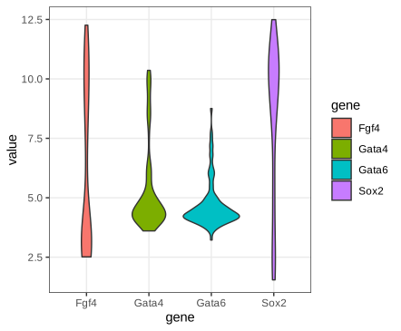
fig_3_20. Reproduces Holmes and Huber (2019), Figure 3.20. PDF · SVG3.6.6 Ridgeline plots
Ridgelines stack the densities vertically with partial overlap. ggridges uses one joint bandwidth for all groups (it reports the value it picks), so the curves are smoothed equally. The layout scales to dozens of groups.
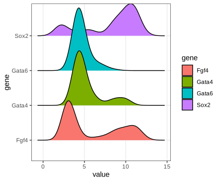
fig_3_21. Reproduces Holmes and Huber (2019), Figure 3.21. PDF · SVG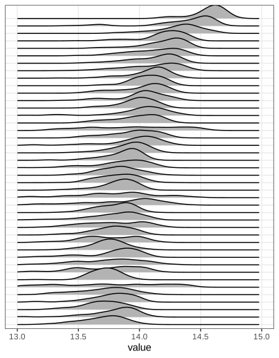
fig_3_22. Reproduces Holmes and Huber (2019), Figure 3.22. PDF · SVG3.6.7 ECDF plots
Definition 3.5 (CDF and empirical CDF) (3.1), (3.2)
The cumulative distribution function of a random variable \(X\) is
\[ F(x)=\Pr(X\le x),\qquad x\in\R. \tag{3.1} \]The empirical cumulative distribution function (ECDF) of a sample \(x_1,\dots,x_n\) is
\[ F_n(x)=\frac{\#\{i:x_i\le x\}}n=\frac1n\sum_{i=1}^n\mathbf 1\{x_i\le x\}. \tag{3.2} \]\(F_n\) is a right-continuous step function, 0 left of \(x_{(1)}\), 1 from \(x_{(n)}\) on, jumping by \(k/n\) at a value that occurs \(k\) times.
Erratum: the indicator in (3.2)
The book's (3.2) writes the indicator as \(\mathbf 1(x\le x_i)\). That counts the observations at or above \(x\) and gives \(1-F_n(x^-)\), a decreasing function, not the ECDF. The argument must be \(x_i\le x\), as in the words before it (“number of \(i\) for which \(x_i\le x\)”). In R, ecdf equals the corrected formula and the literal one equals \(1-F_n(x^-)\).
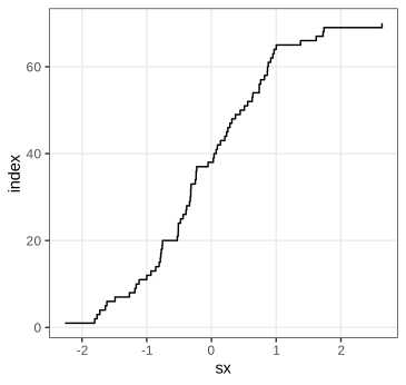
fig_3_23. Reproduces Holmes and Huber (2019), Figure 3.23. PDF · SVGSorting is all it takes: the point \((x_{(i)},i)\) lies on the graph of \(nF_n\). In ggplot2, stat_ecdf does this per group. (The book's Figure 3.25, a panel reprinted from Lawrence et al. 2013 showing mutation frequencies per tumour type as rotated ECDFs, is not reproduced.)
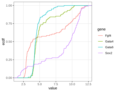
fig_3_24. Reproduces Holmes and Huber (2019), Figure 3.24. PDF · SVGFilling the gap 3.6: why the ECDF is “lossless” and how precise it is Section 3.6.7
The book lists two properties: the ECDF keeps all information except the order of the observations, and it converges to \(F\). Here is the first, with the exact sampling distribution of \(F_n(x)\); Gap 3.7 makes the convergence uniform.
Derivation
Lossless. \(F_n\) jumps exactly at the distinct data values, by \(1/n\) times their multiplicities, so it determines the multiset \(\{x_1,\dots,x_n\}\), equivalently the order statistics, and conversely. For an independent, identically distributed sample with density \(f\), the joint density \(\prod_if(x_i)=\prod_if(x_{(i)})\) depends on the data only through the order statistics, so by the factorisation theorem they are sufficient for \(f\) (for any family of distributions): no inference about \(F\) loses anything by working with \(F_n\). Only the order of collection is discarded, which carries no information when the observations are exchangeable.
Pointwise distribution. For fixed \(x\) the indicators \(\mathbf 1\{X_i\le x\}\) are independent Bernoulli(\(F(x)\)), so
\[ nF_n(x)\sim\mathrm{Bin}\bigl(n,F(x)\bigr),\qquad \E F_n(x)=F(x),\qquad \var F_n(x)=\frac{F(x)\{1-F(x)\}}n . \]\(F_n(x)\) is unbiased, converges almost surely by the strong law of large numbers, and \(\sqrt n\{F_n(x)-F(x)\}\to\N(0,F(x)\{1-F(x)\})\) by the central limit theorem. For \(x\le y\), \(\cov(F_n(x),F_n(y))=\{F(x)-F(x)F(y)\}/n\), since \(\E[\mathbf 1\{X\le x\}\mathbf 1\{X\le y\}]=F(x)\). The variance is largest, \(1/(4n)\), where \(F=1/2\), and vanishes in the tails.
Contrast with densities. The derivative of \(F_n\) is a sum of point masses, useless as a picture; any density estimate must smooth (Gap 3.4), which introduces a bias of order \(h^2\) and a variance of order \(1/(nh)\), worse than the \(1/n\) of \(F_n\). This is the precise sense in which the ECDF is the better-behaved object. ∎
Filling the gap 3.7: uniform convergence (Glivenko–Cantelli), the DKW band and the Kolmogorov–Smirnov distance Section 3.6.7
Result 3.4 (Glivenko–Cantelli; Dvoretzky–Kiefer–Wolfowitz)
For independent \(X_i\) with any CDF \(F\), \(D_n=\sup_x|F_n(x)-F(x)|\to0\) almost surely. Moreover, for every \(\varepsilon>0\) and \(n\),
\[ \Pr(D_n>\varepsilon)\le2e^{-2n\varepsilon^2} \](Dvoretzky, Kiefer and Wolfowitz 1956, with the constant 2 due to Massart 1990). Hence \(F_n\pm\varepsilon_n\), \(\varepsilon_n=\sqrt{\ln(2/\alpha)/(2n)}\), clipped to \([0,1]\), is a confidence band that contains the whole of \(F\) with probability at least \(1-\alpha\), for every \(F\).
Proof of Glivenko–Cantelli, and the band
Fix an integer \(k\) and let \(t_j=Q(j/k)\) for \(j=1,\dots,k-1\), \(t_0=-\infty\), \(t_k=+\infty\). By the definition of \(Q\), \(F(t_j^-)\le j/k\le F(t_j)\), so for consecutive points \(F(t_j^-)-F(t_{j-1})\le j/k-(j-1)/k=1/k\). For \(x\in[t_{j-1},t_j)\), monotonicity of \(F_n\) and \(F\) gives
\[ F_n(x)-F(x)\le F_n(t_j^-)-F(t_{j-1})\le F_n(t_j^-)-F(t_j^-)+\tfrac1k, \] \[ F_n(x)-F(x)\ge F_n(t_{j-1})-F(t_j^-)\ge F_n(t_{j-1})-F(t_{j-1})-\tfrac1k. \]So \(D_n\le\max_j\max\{|F_n(t_j)-F(t_j)|,|F_n(t_j^-)-F(t_j^-)|\}+1/k\). The maximum is over finitely many points, at each of which the strong law gives almost sure convergence (\(F_n(t^-)\) is an average of the indicators \(\mathbf 1\{X_i<t\}\)). Hence \(\limsup_nD_n\le1/k\) almost surely; intersect these events over \(k=1,2,\dots\) to get \(D_n\to0\) almost surely.
The band. Set \(2e^{-2n\varepsilon^2}=\alpha\). Then \(\Pr(\sup_x|F_n(x)-F(x)|\le\varepsilon_n)\ge1-\alpha\), and \(|F_n(x)-F(x)|\le\varepsilon_n\) for all \(x\) is exactly \(F\) lying in the band. For the 101 cells and \(\alpha=0.05\), \(\varepsilon=\sqrt{\ln40/202}=0.135\): a wide band, which is the honest price of making no assumption about \(F\). (The proof of the DKW inequality itself is long; see Massart 1990.)
Distribution-free. If \(F\) is continuous, \(U_i=F(X_i)\) are uniform on (0,1) (Gap 3.8), \(F_n(x)=G_n(F(x))\) with \(G_n\) the ECDF of the \(U_i\), and since \(F\) maps \(\R\) onto (0,1) up to endpoints, \(D_n=\sup_u|G_n(u)-u|\): its distribution does not depend on \(F\). This is what makes the Kolmogorov–Smirnov test possible. The supremum is attained at the jumps, so
\[ D_n=\max_{1\le i\le n}\max\Bigl\{\frac in-F(x_{(i)}),\;F(x_{(i)})-\frac{i-1}n\Bigr\}, \]which agrees with ks.test. \(\sqrt nD_n\) converges to the supremum of the absolute value of a Brownian bridge (Kolmogorov's distribution). If \(F\) is a normal with mean and standard deviation estimated from the same data, \(D_n\) is stochastically smaller and the standard p-values are too large (Lilliefors' correction is needed). ∎
Filling the gap 3.8: quantile functions, the probability integral transform and QQ plots Sections 3.6.2, 3.6.7
The ECDF plots \(p\) against \(x\); a quantile-quantile (QQ) plot compares two distributions through their quantile functions instead. The facts it rests on:
Derivation
Galois inequality. For \(0<p<1\) and real \(x\): \(Q(p)\le x\iff p\le F(x)\). If \(p\le F(x)\) then \(x\) is in the set \(\{y:F(y)\ge p\}\), whose infimum is \(Q(p)\), so \(Q(p)\le x\). Conversely, the set is an interval \([Q(p),\infty)\) (closed on the left because \(F\) is right-continuous), so \(Q(p)\le x\) implies \(F(x)\ge F(Q(p))\ge p\).
Inverse transform. If \(U\sim\) Uniform(0,1), then \(\Pr(Q(U)\le x)=\Pr(U\le F(x))=F(x)\): \(Q(U)\) has CDF \(F\). Probability integral transform. If \(F\) is continuous, \(F(X)\sim\) Uniform(0,1): for \(u\in(0,1)\), \(\Pr(F(X)\ge u)=\Pr(X\ge Q(u))=1-F(Q(u)^-)=1-u\), because continuity gives \(F(Q(u))=u\) and \(\Pr(X=Q(u))=0\).
Equivariance. If \(g\) is increasing and continuous, \(Q_{g(X)}(p)=g(Q_X(p))\): quantiles, unlike means and modes (Gap 3.9), commute with monotone transformations.
QQ plot. Plot the order statistics \(x_{(i)}\) against reference quantiles \(Q_0(p_i)\). By the inverse transform, \(x_{(i)}\) is distributed as \(Q(U_{(i)})\), and \(\E U_{(i)}=i/(n+1)\), so \(x_{(i)}\approx Q(p_i)\) for plotting positions near \(i/(n+1)\); R's ppoints uses \((i-a)/(n+1-2a)\) with \(a=3/8\) for \(n\le10\) and \(a=1/2\) otherwise. If \(F\) belongs to the location-scale family of \(F_0\), \(F(x)=F_0((x-\mu)/\sigma)\), then \(Q(p)=\mu+\sigma Q_0(p)\): the points lie near a straight line with slope \(\sigma\) and intercept \(\mu\), whatever \(\mu,\sigma\) are. qqline draws the line through the quartile pairs, slope \(\operatorname{IQR}/(z_{0.75}-z_{0.25})=\operatorname{IQR}/1.349\), a robust estimate of \(\sigma\) under normality. Departures have shapes: heavier tails than the reference bend the ends away from the line (an S), right skew makes the plot convex, and a gap between two modes appears as a steep jump between two flatter runs, as for Fgf4 (slope 4.87 and intercept 6.24 for its quartile line). ∎
Task (tibbles)
A tibble is a data frame that prints only the first rows and the column types, never converts strings to factors, does not partially match column names, and keeps non-syntactic names such as `59 E4.5 (PE)` as they are. vignette("tibble") lists the differences.
3.6.8 The effect of transformations on densities
Bimodality in a histogram is tempting to interpret biologically, but the number of modes depends on the scale. Array 64 (an E4.5 EPI cell) has two clear modes on the stored log2 scale and none after the first when its values are put back on the fluorescence scale (Holmes and Huber 2019, Section 3.6.8).
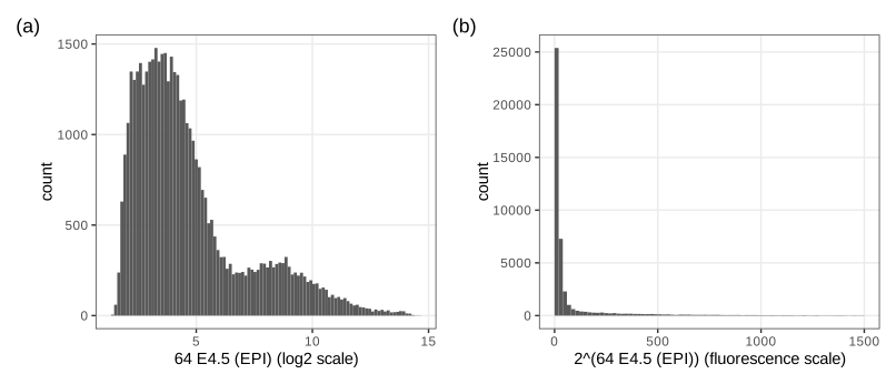
fig_3_26. Reproduces Holmes and Huber (2019), Figure 3.26. PDF · SVGQuestion 3.5 (densities and modes under a transformation)
Let \(f\) be a non-linear one-to-one transformation and \(Y=f(X)\) with density \(p\). What is the density of \(X\)? How are the modes of \(X\) and \(Y\) related; is \(f(x_0)\) a mode of \(Y\) when \(x_0\) is a mode of \(X\)?
Answer
See Result 3.5 below: \(\tilde p(x)=p(f(x))\,|f'(x)|\); its stationary points satisfy \(p'(f(x))f'(x)^2+p(f(x))f''(x)=0\) (for increasing \(f\)), so a mode of \(X\) maps to a mode of \(Y\) only where \(f''=0\). In general there is no correspondence: modes can move, appear and disappear. (The book's solution omits the absolute value, which matters for decreasing \(f\).)
Filling the gap 3.9: the change-of-variables formula, and why modes are not preserved Section 3.6.8, Question 3.5
Result 3.5 (densities under a monotone transformation)
Let \(X\) have density \(p_X\) on an open interval \(I\), and let \(f:I\to J\) be a bijection, continuously differentiable with \(f'\ne0\). Then \(Y=f(X)\) has density \(p_Y(y)=p_X(f^{-1}(y))\,|(f^{-1})'(y)|\), equivalently \(p_X(x)=p_Y(f(x))\,|f'(x)|\). If \(p_Y\) and \(f\) are twice differentiable and \(f\) is increasing, the stationary points of \(p_X\) solve \(p_Y'(f(x))f'(x)^2+p_Y(f(x))f''(x)=0\).
Proof and two examples
\(f'\) is continuous and never zero, so it has one sign: \(f\) is strictly monotone. If increasing, \(F_Y(y)=\Pr(f(X)\le y)=F_X(f^{-1}(y))\); differentiate (chain rule, inverse function theorem): \(p_Y(y)=p_X(f^{-1}(y))(f^{-1})'(y)\). If decreasing, \(F_Y(y)=1-F_X(f^{-1}(y))\) and the derivative carries a minus sign, which together with \((f^{-1})'<0\) gives the absolute value. Since \((f^{-1})'(f(x))=1/f'(x)\), the second form follows. Differentiating \(p_X(x)=p_Y(f(x))f'(x)\) by the product and chain rules gives the stationarity condition. At a mode \(x_0\) of \(X\), \(p_Y'(f(x_0))=-p_Y(f(x_0))f''(x_0)/f'(x_0)^2\), which is non-zero unless \(f''(x_0)=0\): \(f(x_0)\) is not a stationary point of \(p_Y\). Only affine maps preserve modes in general. ∎
Lognormal. If \(X\sim\N(\mu,\sigma^2)\) and \(Y=e^X\), then \(p_Y(y)=\phi((\ln y-\mu)/\sigma)/(\sigma y)\) and \(\frac{\d}{\d y}\ln p_Y=-\frac{\ln y-\mu}{\sigma^2y}-\frac1y\), zero at \(\ln y=\mu-\sigma^2\). The mode of \(Y\) is \(e^{\mu-\sigma^2}\), below \(e^\mu=e^{\text{mode of }X}\), which is the median of \(Y\) (quantiles are equivariant), itself below the mean \(e^{\mu+\sigma^2/2}\).
Array 64. Let \(p\) be the density on the log2 scale and \(y=2^x\). Then \(q(y)=p(\log_2y)/(y\ln2)\) and, writing \(x=\log_2y\), \(\frac{\d}{\d x}\ln q=(\ln p)'(x)-\ln2\). Since \(x\) increases with \(y\), \(q\) has a local maximum only where \((\ln p)'\) falls through \(\ln2=0.693\). The kernel estimate of \(p\) has modes at 3.39 and 8.69; on the rising flank of the second bump \((\ln p)'\) never exceeds 0.30, so that bump leaves no mode on the fluorescence scale, and the first mode moves from \(2^{3.39}\) to \(2^{2.21}=4.6\) (checked in R). Figure 3.26(b) shows exactly this.
3.7 Visualizing data in 2D: scatterplots
Scatterplots show treatment against response, association, or paired measurements. Two arrays of the Hiiragi data, cell 59 (E4.5, PE) and cell 92 (E4.5, FGF4-KO), give 45,101 points, far more than a scatterplot can show individually (Holmes and Huber 2019, Section 3.7).
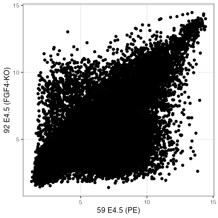
fig_3_27. Reproduces Holmes and Huber (2019), Figure 3.27. PDF · PNGSemi-transparency helps up to a point: a pixel covered by \(k\) points of opacity \(\alpha\) has opacity \(1-(1-\alpha)^k\). With \(\alpha=0.1\) it is 0.65 at \(k=10\) and 0.995 at \(k=50\), so every region with more than a few dozen overlapping points looks equally black, while an isolated point keeps only opacity 0.1.
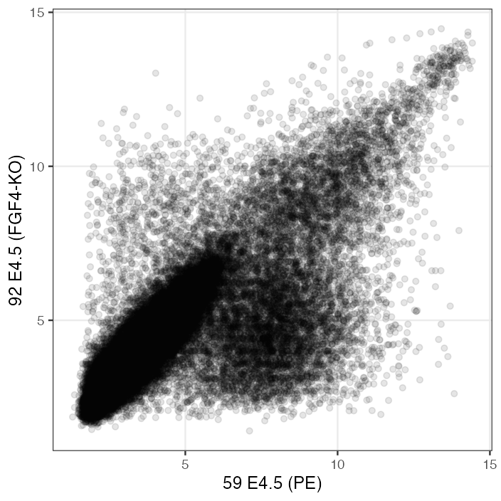
fig_3_28. Reproduces Holmes and Huber (2019), Figure 3.28. PDF · PNG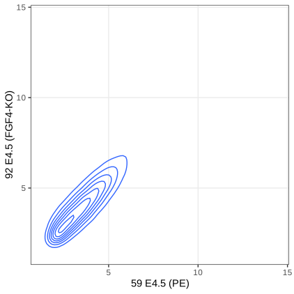
fig_3_29. Reproduces Holmes and Huber (2019), Figure 3.29. PDF · SVG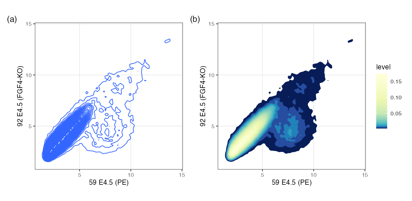
h = 0.5, a kernel standard deviation of 0.125) and 60 contour levels. (b) The regions between contours filled by level, with equal units on both axes. Contours computed with MASS::kde2d and contourLines (see the code). Code: fig_3_30. Reproduces Holmes and Huber (2019), Figure 3.30. PDF · PNGFilling the gap 3.10: what the 2-D density contours are, and what “h = 0.5” means Section 3.7, Figures 3.29, 3.30
geom_density2d and stat_density2d call MASS::kde2d: a product-kernel estimate on a 100 × 100 grid over the data range,
Details
The factor 4. In kde2d the argument h is four times the kernel standard deviation (this formula reproduces kde2d's grid maximum to \(10^{-14}\)). Its default, bandwidth.nrd, is \(4\times1.06\min(s,\operatorname{IQR}/1.34)n^{-1/5}\), i.e. the one-dimensional normal reference rule of Gap 3.5 in each coordinate: 1.036 and 0.821 here, kernel standard deviations 0.26 and 0.21. The book's h = c(0.5, 0.5) means a kernel standard deviation of 0.125, about half the default, which is why Figure 3.30 resolves more structure.
Rates in \(d\) dimensions. The argument of Result 3.2 carries over: the bias is \(\tfrac12\sum_jh_j^2\partial_j^2f+o(h^2)\) and the variance \(R(K)^df/(nh_1\cdots h_d)\). With a common \(h\), \(\mathrm{AMISE}=c_1h^4+c_2/(nh^d)\), minimised at \(h\propto n^{-1/(d+4)}\) with error of order \(n^{-4/(d+4)}\): \(n^{-2/3}\) in two dimensions against \(n^{-4/5}\) in one. The per-coordinate rule above uses the exponent \(-1/5\) of one dimension and therefore undersmooths slightly for large \(n\). Densities get harder to estimate as \(d\) grows (see also Gap 3.18).
Contours. A contour line is a level set \(\{\hat f=c\}\); ggplot2 places the levels at pretty(range, 10) by default, or at about bins equally spaced levels. The region \(\{\hat f\ge c\}\) is a highest-density region: among all regions with the same probability under \(\hat f\) it has the smallest area. Because contours only show where density is high, the sparse cloud at the lower right of Figure 3.29 vanishes: its density is below the lowest level. Drawing the points that lie below the lowest contour, as the book suggests, restores them.
Hexagonal binning (Carr et al. 1987) counts points in a tiling of the plane and colours each tile by its count: a two-dimensional histogram, with no smoothing and nothing hidden.
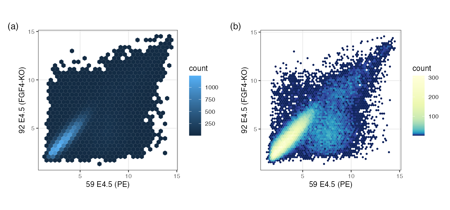
fig_3_31. Reproduces Holmes and Huber (2019), Figure 3.31. PDF · PNGAlgorithm 3.2 (hexagonal binning as in geom_hex/hexbin) Section 3.7, Figure 3.31
- Choose widths \(w_x,w_y\). Lattice centres: columns \(w_x\) apart, rows \(w_y\sqrt3/2\) apart, every second row shifted by \(w_x/2\); the origin is the data minimum rounded down to a multiple of the width.
- In scaled coordinates \(s_x=(x-x_0)/w_x\), \(s_y=(y-y_0)/(w_y\sqrt3)\) the centres form two rectangular lattices: integer points \((j,i)\) and the points \((j+\frac12,i+\frac12)\). Assign each point to the nearer of its candidate centre in each lattice, distances measured as \((s_x-j)^2+3(s_y-i)^2\) (Euclidean distance in the unscaled hexagonal geometry).
- Count the points per cell and draw each non-empty hexagon coloured by its count.
Filling the gap 3.11: hexagon counts as a density estimate, and why hexagons Section 3.7
Derivation
Nearest-centre cells are hexagons. In the scaled metric the centres form a triangular lattice in which each centre has six nearest neighbours at equal distance; the set of points closer to one centre than to any other (its Voronoi cell) is bounded by the six perpendicular bisectors, a regular hexagon. The two-lattice rule of Algorithm 3.2 finds the nearest centre because the nearest centre is always one of the rounded positions in the two rectangular sublattices.
Counts. The cell counts \((N_1,\dots,N_m)\) are multinomial with probabilities \(p_j=\int_{C_j}f\). The estimate \(\hat f=N_j/(nA)\) on cell \(C_j\), where \(A=w_x\cdot w_y\sqrt3/2\) is the cell area, has mean \(p_j/A\), the average of \(f\) over the cell, equal to \(f(c_j)+O(w^2)\) at the centre \(c_j\) by a second-order Taylor expansion (the cell is symmetric about \(c_j\), so the linear term integrates to zero), and variance \(p_j(1-p_j)/(nA^2)\approx f(c_j)/(nA)\). This is the bias-variance trade-off of Gap 3.4 with the bin width in place of \(h\).
Why hexagons. Representing every point of a cell by its centre costs the mean squared distance \(\frac1A\int_C\|\mathbf u-\mathbf c\|^2\,\d\mathbf u=2GA\), with \(G\) the dimensionless second moment of the cell. For a square of side \(a\): \(\int\|\mathbf u\|^2=a^4/6\), so \(G=\frac{a^4/6}{2a^4}=\frac1{12}=0.0833\). For a regular hexagon of side \(s\): area \(\frac{3\sqrt3}2s^2\) and polar moment \(\frac{5\sqrt3}8s^4\), so \(G=\frac{5\sqrt3/8}{2\cdot27/4}=\frac5{36\sqrt3}=0.0802\). Among the three regular tilings of the plane the hexagon is the roundest; at equal area it represents the points about 4% more accurately than squares, and it avoids the horizontal and vertical lines that square bins impose on the picture.
For the two arrays with width 0.2 (Figure 3.31b), 2,796 hexagons are non-empty and the largest holds 309 probes (on the exported data rounded to three decimals; 2,797 and 309 at full precision), reproduced exactly by the demonstration. ∎
3.7.1 Plot shapes
The shape of a plot is a choice. Two rules: if both axes have the same units (both log2 expression, or two principal components), use the same scale on both, coord_fixed(); PCA plots are then wider than tall because the first component has the largest variance. If the units differ, choose the aspect ratio from the data, for example by banking (Cleveland et al. 1988).
Algorithm 3.3 (banking to 45°) Section 3.7.1, Figure 3.32
For a curve through \((x_i,y_i)\), compute the segment slopes \(s_i=(y_{i+1}-y_i)/(x_{i+1}-x_i)\). Choose the number \(r\) of page units per \(y\) unit, relative to one page unit per \(x\) unit, so that the median of \(|s_i|\) is drawn at 45°: \(r=1/\operatorname{median}|s_i|\), i.e. coord_fixed(ratio = r).
Filling the gap 3.12: why 45°, and what bank_slopes returns Section 3.7.1
Derivation, and a correction
A segment of data slope \(s\) drawn with \(a\) page units per \(x\) unit and \(b\) per \(y\) unit has page slope \(sb/a\). coord_fixed(ratio = r) sets \(b/a=r\), so the page slope is \(rs\), and the median page slope is 1 exactly when \(r=1/\operatorname{median}|s|\). Cleveland, McGill and McGill (1988) found that people compare the slopes of two segments most accurately when their orientations are centred on 45°; banking makes the typical segment sit there. For the sunspots the median absolute slope is 14.5 numbers per year, so \(r=0.069\), and the plot is very flat (Figure 3.32b): the rapid rise and slow decay of each cycle become visible.
Correction. The book passes ggthemes::bank_slopes(year, number) to coord_fixed. That function returns \(R_y/(R_x\operatorname{median}|s|)\), with \(R_x,R_y\) the data ranges: the panel aspect ratio (height/width) that banks the curve, which belongs in theme(aspect.ratio = ...). Read as y-per-x units, it gives the median page slope \(R_y/R_x=0.66\), i.e. 33°, not 45° (ratio 0.0456 instead of 0.0690; verified in R). Figure 3.32(b) here uses \(r=1/\operatorname{median}|s|\); the picture differs from the book's only in being 1.5 times taller. ∎
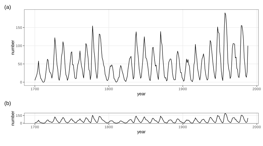
fig_3_32. Reproduces Holmes and Huber (2019), Figure 3.32. PDF · SVG3.8 Visualizing more than two dimensions
geom_point has further aesthetics, fill, color, shape, size and alpha, each of which can carry one more variable. Using all of them at once gives an unreadable plot; one or two extra variables are usually the limit (Holmes and Huber 2019, Section 3.8).
3.8.1 Faceting
Faceting (trellis or lattice graphics) repeats the same plot for subsets defined by one or two more variables, with shared axes so the panels can be compared. facet_grid(rows ~ cols) lays out a grid; facet_wrap(~ v) wraps one variable's panels into rows.
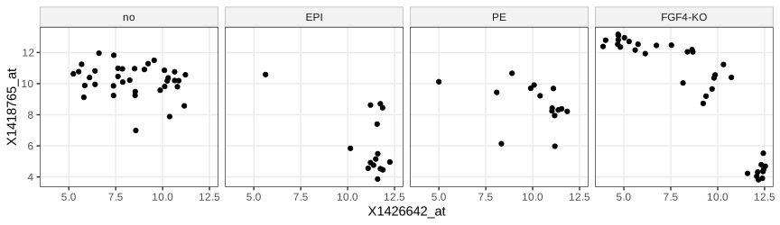
lineage (cells without a lineage label are "no"). Code: fig_3_33. Reproduces Holmes and Huber (2019), Figure 3.33. PDF · SVG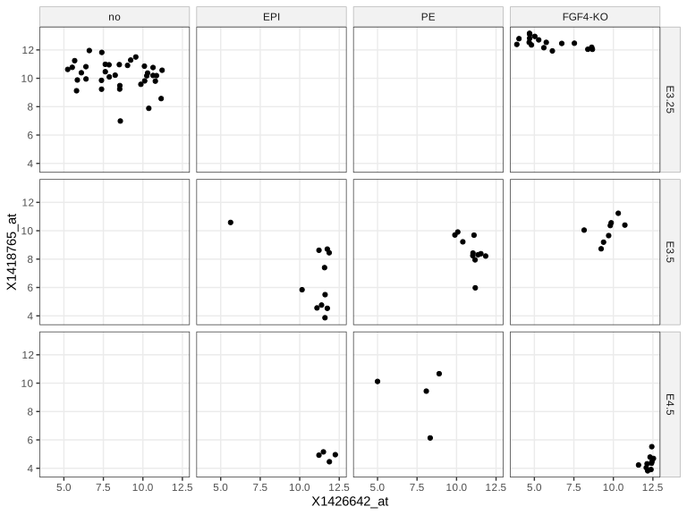
fig_3_34. Reproduces Holmes and Huber (2019), Figure 3.34. PDF · SVG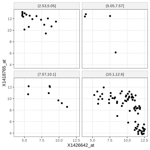
cut(..., breaks = 4)), so the panels hold different numbers of cells. Code: fig_3_35. Reproduces Holmes and Huber (2019), Figure 3.35. PDF · SVGcut(v, breaks = 4) splits the range of v into four intervals of equal length, so the panels hold different numbers of cells (here mostly the lowest interval). Equal-count panels need quantile breaks, cut(v, quantile(v, 0:4/4), include.lowest = TRUE), whose expected counts are \(n/4\) each, or a cut of rank(v). Axis scales. scales = "free" (or "free_x", "free_y") lets each panel use its own range: more detail per panel, less comparability across panels. Implicit faceting. A factor mapped to x, as in Figures 3.15–3.18, is already a form of faceting.
3.8.2 Interactive graphics
shiny builds web applications whose controls call back into a running R session that redraws the plot; ggvis extended the grammar of graphics to interactive, browser-rendered graphics (Vega) but its development stopped; plotly produces self-contained HTML/JavaScript graphics that need no R session (plotly::ggplotly converts a ggplot); rgl renders rotatable 3-D scenes with OpenGL or WebGL. The demonstrations of this course are of the self-contained kind. The volcano scene of the book's Figure 3.36 needs a display device; here the same surface and colour map are drawn statically.
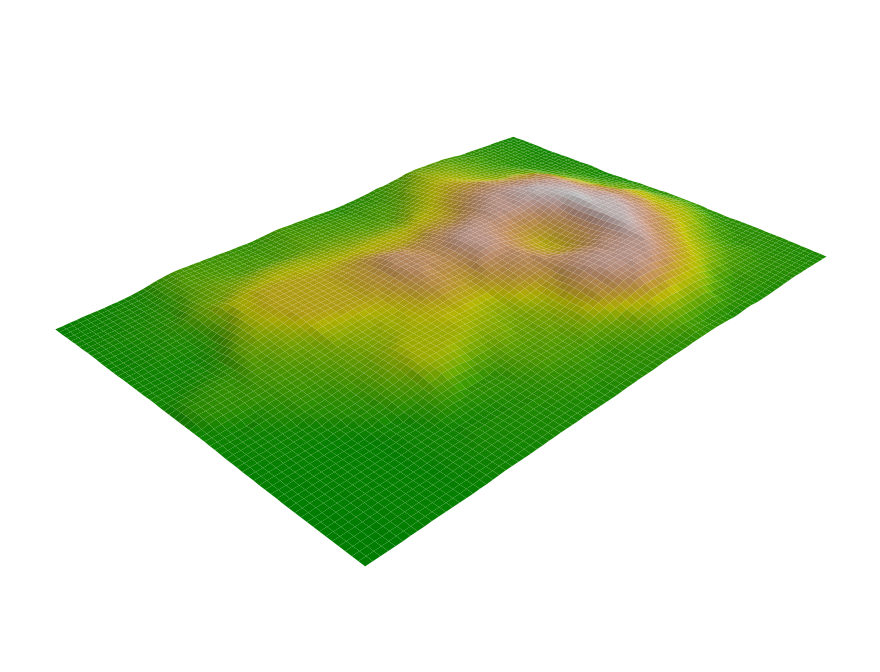
volcano elevation grid (10 m spacing) with the 500-step terrain.colors map. The book shows an interactive rgl scene; this static persp() view of the same surface stands in for it. Code: fig_3_36. Reproduces Holmes and Huber (2019), Figure 3.36. PDF · PNG3.9 Color
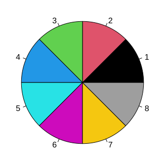
fig_3_37. Reproduces Holmes and Huber (2019), Figure 3.37. PDF · SVGNote on Figure 3.37 and its footnote
The book explains the base palette as the eight corners of the RGB cube (black, red, green, blue, cyan, magenta, yellow, and grey instead of white). That was R's palette before version 4.0. Since R 4.0 the default is "black" "#DF536B" "#61D04F" "#2297E6" "#28E2E5" "#CD0BBC" "#F5C710" "gray62", chosen for more even luminance; the figure produced by current R (and shown here) uses it. palette("R3") restores the old one.
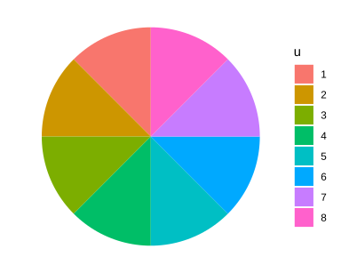
fig_3_38. Reproduces Holmes and Huber (2019), Figure 3.38. PDF · SVGRColorBrewer offers designed palettes in three kinds: qualitative for unordered categories (Paired has 12 colours in 6 light/dark pairs, for categories with two sub-categories), sequential for ordered quantities from low to high, and diverging for quantities with a meaningful midpoint, such as fold changes around 0 (Figure 3.41). brewer.pal(4, "RdYlGn") returns "#D7191C" "#FDAE61" "#A6D96A" "#1A9641".
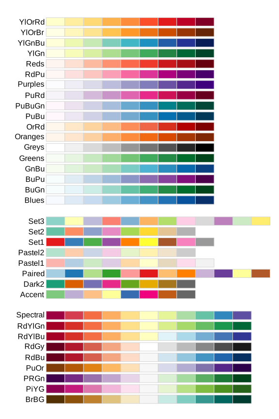
fig_3_39. Reproduces Holmes and Huber (2019), Figure 3.39. PDF · SVGcolorRampPalette(cols)(m) returns a function value: \(m\) colours obtained by linear interpolation of the red, green and blue channels between consecutive anchors. With anchors darkorange3 (205, 102, 0), white and darkblue, the first steps are #CD6600, #CE6905, #CF6C0A, as the book prints (checked). Interpolation in RGB is simple but not perceptually even (Gap 3.15).
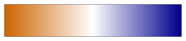
colorRampPalette(c("darkorange3", "white", "darkblue"))(100): 100 colours interpolated linearly in RGB between three anchors. Code: fig_3_40. Reproduces Holmes and Huber (2019), Figure 3.40. PDF · PNG3.10 Heatmaps
A heatmap shows a matrix as coloured cells, with rows and columns reordered so that similar ones are adjacent. The book uses pheatmap on the 500 probes with the largest variance across the 101 cells, each centred at its row mean, with breaks from \(-5\) to 5 and annotation bars for sample group, embryonic day, scan date and genotype (Holmes and Huber 2019, Section 3.10).
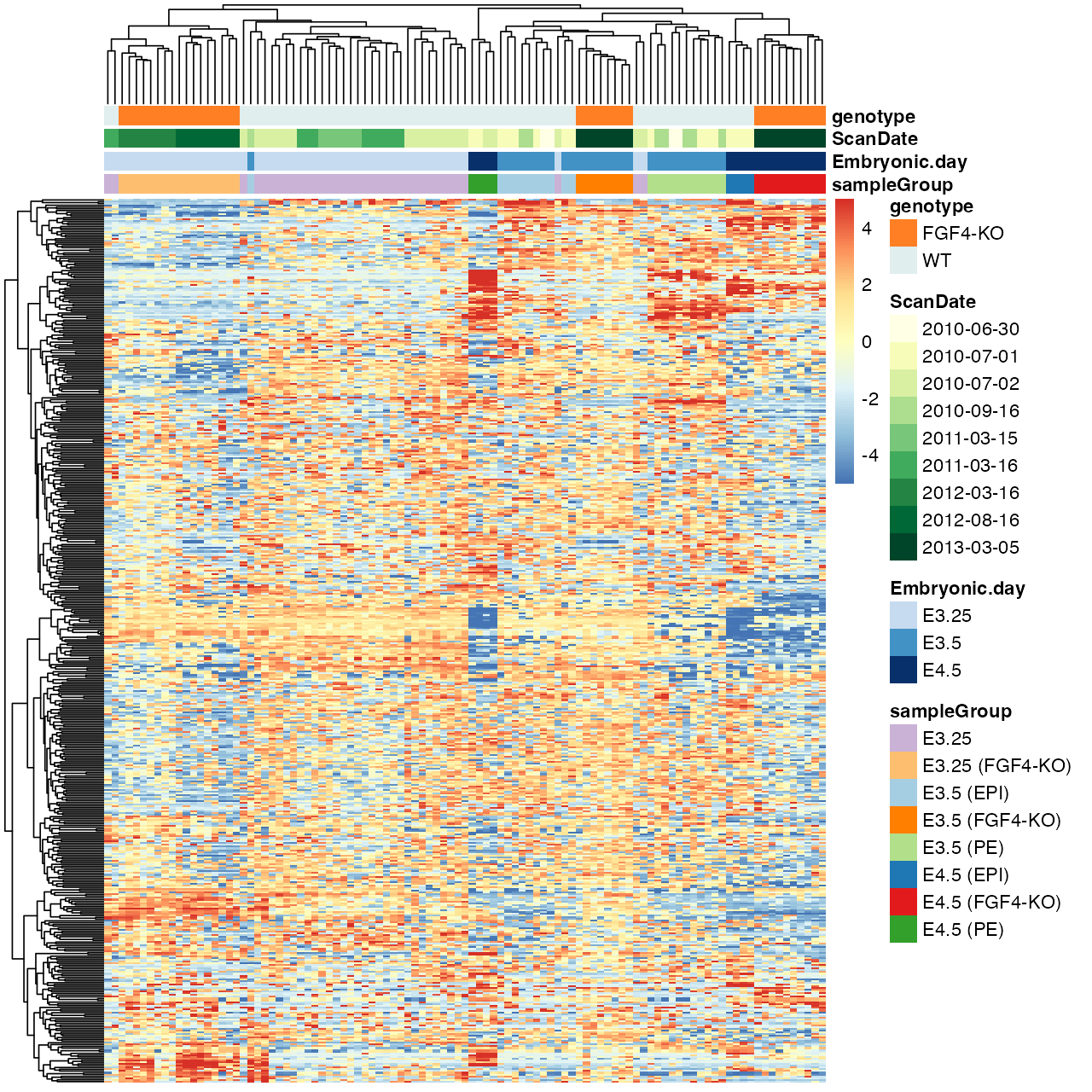
fig_3_41. Reproduces Holmes and Huber (2019), Figure 3.41. PDF · PNGFilling the gap 3.13: what the colours of Figure 3.41 measure Section 3.10
Details
The entries are \(z_{gi}=\log_2I_{gi}\), with \(I_{gi}\) the (RMA-summarised) intensity of probe \(g\) in cell \(i\). After centring, \(z_{gi}-\bar z_{g\cdot}=\log_2\bigl(I_{gi}/\tilde I_g\bigr)\), where \(\tilde I_g=(\prod_iI_{gi})^{1/101}\) is the geometric mean of the probe's intensities: each cell shows the log2 fold change of the probe relative to its own typical level, so a diverging palette with 0 at the neutral colour is the right choice, and probes with very different absolute levels become comparable. Selecting the 500 probes with the largest variance keeps those that vary across cells; it favours probes with large fold changes and does not account for the probe's measurement noise.
Rows and columns are ordered by complete-linkage hierarchical clustering of Euclidean distances (pheatmap's default; Chapter 5). breaks fixes the map from values to the 100 colours, so the colour scale is symmetric about 0 whatever the data range. The book says pheatmap's default palette interpolates the 11 colours of RdYlBu; the default is colorRampPalette(rev(brewer.pal(n = 7, name = "RdYlBu")))(100), seven colours (checked against the installed pheatmap).
3.10.1 Dendrogram ordering
The visual impression of a heatmap depends heavily on the ordering, and dendrogram ordering is only one choice; even then each internal branch can be flipped without changing the tree.
Filling the gap 3.14: how many orderings one dendrogram allows Section 3.10.1
Result 3.6
A rooted binary tree with \(n\) leaves admits exactly \(2^{n-1}\) left-to-right leaf orders, one for each choice of flipping or not flipping each of its \(n-1\) internal nodes.
Proof
A rooted binary tree with \(n\) leaves has \(n-1\) internal nodes (induction: merging two subtrees with \(n_1\) and \(n_2\) leaves adds one node, \((n_1-1)+(n_2-1)+1=n-1\)). A drawing is fixed by deciding, at each internal node, which child goes left: \(2^{n-1}\) choices, and each gives a leaf order in which every subtree's leaves are contiguous. Different choices give different orders: take an internal node \(v\) where the two choices differ; in one drawing all leaves of \(v\)'s first child precede those of its second, in the other they follow them, so any leaf pair \((a,b)\) with \(a,b\) in the two children appears in opposite orders. Hence there are exactly \(2^{n-1}\) orders (enumeration confirms all 16 for a 5-leaf tree). For the 101 cells that is \(2^{100}\approx1.3\times10^{30}\) orders, out of \(101!\approx9.4\times10^{159}\). ∎
Question 3.6 (which branch goes left?)
How does pheatmap decide which subtree is drawn on the left?
Answer
It uses the order stored by hclust. As documented in ?hclust, at each merge the tighter cluster (the one whose own last merge happened at the lower height) is put on the left; single observations count as tightest, and two observations merged together appear in the order of their indices.
Question 3.7 (other orderings)
What other ways of ordering rows and columns are there?
Answer
Seriation: order by the first principal component (or the angle in the plane of the first two); solve a travelling-salesman problem that minimises the sum of distances between neighbours (McCormick et al. 1972); among the \(2^{n-1}\) orders of Result 3.6, choose the one that minimises the sum of distances between adjacent leaves (optimal leaf ordering, which can be found by dynamic programming); or order by a known covariate such as time or group.
Question 3.8 (clustering_callback)
What does pheatmap's clustering_callback do?
Answer
It is a function function(hc, mat) called with each hclust result and the matrix it came from; it must return an hclust object, whose order pheatmap then uses. Example: reorder the tree by the first principal component, function(hc, mat) { sv = svd(t(mat))$v[, 1]; as.hclust(reorder(as.dendrogram(hc), wts = sv)) }. The tree topology stays; only the flips change.
3.10.2 Color spaces
Human colour vision is three-dimensional (Helmholtz 1867), so every colour model uses three coordinates. In RGB, groupColor[1] = "#CAB2D6" has red, green and blue channel values CA, B2, D6 in hexadecimal, i.e. 202, 178, 214 out of 255, a point in the unit cube after division by 255. hcl() uses hue \(H\) (an angle), chroma \(C\) and luminance \(L\in[0,100]\), the polar coordinates of the CIELUV space.
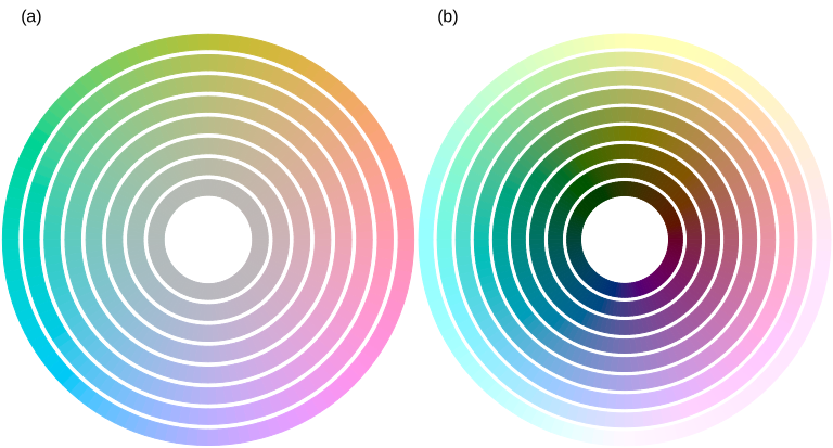
fig_3_42. Reproduces Holmes and Huber (2019), Figure 3.42. PDF · SVGFilling the gap 3.15: from a hex code to HCL, and why HCL is used for palettes Section 3.10.2
The conversion
sRGB channel values \(c\in[0,1]\) are gamma-encoded; linear light is \(c_{\mathrm{lin}}=c/12.92\) for \(c\le0.04045\) and \(((c+0.055)/1.055)^{2.4}\) otherwise. A fixed matrix (for the D65 white point) maps linear RGB to the CIE XYZ tristimulus values, \(Y\) being luminance. CIELUV then sets
\[ L^*=116\,(Y/Y_n)^{1/3}-16\ \ (Y/Y_n>(6/29)^3),\qquad u^*=13L^*(u'-u'_n),\quad v^*=13L^*(v'-v'_n), \]with chromaticities \(u'=4X/(X+15Y+3Z)\), \(v'=9Y/(X+15Y+3Z)\) and \(n\) denoting the white point. HCL is the polar form: \(L=L^*\), \(C=\sqrt{u^{*2}+v^{*2}}\), \(H=\operatorname{atan2}(v^*,u^*)\) in degrees. The cube root makes \(L^*\) roughly proportional to perceived lightness, and the space was designed so that Euclidean distances approximate perceived colour differences far better than distances in RGB. Inverting these formulas by hand (HCL \(\to\) LUV \(\to\) XYZ \(\to\) sRGB) agrees with grDevices::hcl to the last of 255 levels. Not every \((H,C,L)\) is displayable: the largest chroma depends on hue and luminance, which is why the outer rings of Figure 3.42 differ in saturation across hues.
Consequences for palettes (Ihaka 2003; Zeileis et al. 2009). Colours of equal \(L\) and \(C\) differing only in \(H\) are equally light and equally vivid, so no category draws more attention than another and no area looks larger (ggplot2's default discrete palette, Figure 3.38). Sequential palettes should change \(L\) monotonically, so that order survives printing in grey and most colour-vision deficiencies; diverging palettes run two hues out from a light neutral centre. Linear interpolation in RGB (Figure 3.40) does not keep \(L\) monotone in general.
Note on Figure 3.42. The book's caption gives chroma 0, 10, ..., 60 at luminance 75 in (a), and luminance 10, ..., 90 at chroma 50 in (b); its code (reproduced here) uses chroma 5, 15, ..., 75 at luminance 75, and luminance 20, ..., 100 at chroma 55. ∎
Choosing hues. Triads are three hues 120° apart, tetrads four hues 90° apart, analogous colours a short arc of the wheel, complementary colours opposite hues, and split complementaries one hue with the two hues 30° either side of its complement (for two similar categories and a contrasting third). Lines versus areas. Lines and points need strong contrast with the background (dark, low \(L\), on white); large areas look better in light colours of low to moderate chroma.
3.11 Data transformations
When most points crowd into a small part of the plot, a transformation can spread them. The logarithm is the usual choice for intensities: equal steps on the log scale are equal fold changes, \(\log(ax)=\log a+\log x\). It fails for zero or negative values and can over-expand the low end, where additive noise dominates (Holmes and Huber 2019, Section 3.11).
Filling the gap 3.16: the delta method and variance-stabilising transformations Section 3.11
Result 3.7 (delta method)
If \(\sqrt n(T_n-\mu)\to\N(0,v(\mu))\) in distribution and \(g\) is differentiable at \(\mu\), then \(\sqrt n(g(T_n)-g(\mu))\to\N(0,g'(\mu)^2v(\mu))\). For a single measurement with small relative noise, the same expansion gives \(\var g(X)\approx g'(\mu)^2v(\mu)\) with \(\mu=\E X\), \(v(\mu)=\var X\).
Proof and the stabilising transformations
Define \(r(t)=(g(t)-g(\mu))/(t-\mu)-g'(\mu)\) for \(t\ne\mu\) and \(r(\mu)=0\); differentiability means \(r\) is continuous at \(\mu\). Then \(\sqrt n(g(T_n)-g(\mu))=\{g'(\mu)+r(T_n)\}\sqrt n(T_n-\mu)\). Since \(\sqrt n(T_n-\mu)\) converges in distribution, \(T_n\to\mu\) in probability, so \(r(T_n)\to0\) in probability (continuous mapping), and Slutsky's lemma gives the limit \(g'(\mu)\N(0,v(\mu))\). ∎
Stabilising. If \(\var X=v(\mu)\) depends on the mean, choose \(g\) with \(g'(\mu)=1/\sqrt{v(\mu)}\), i.e. \(g(x)=\int^x\d t/\sqrt{v(t)}\); then \(\var g(X)\approx1\) at every level:
- Poisson, \(v=\mu\): \(g(x)=2\sqrt x\) (sd \(\to1\); Anscombe 1948 refined it to \(2\sqrt{x+3/8}\)).
- Pure multiplicative noise, \(v=b^2\mu^2\): \(g(x)=\log(x)/b\).
- Negative binomial (gamma-Poisson), \(v=\mu+\alpha\mu^2\): \(\int\d t/\sqrt{t+\alpha t^2}=\frac2{\sqrt\alpha}\operatorname{asinh}\sqrt{\alpha x}\) (differentiate: \(\frac2{\sqrt\alpha}\cdot\frac{\sqrt\alpha/(2\sqrt x)}{\sqrt{1+\alpha x}}=\frac1{\sqrt{x+\alpha x^2}}\)).
- Additive plus multiplicative noise, \(v=a^2+b^2\mu^2\) (microarrays; Rocke and Durbin 2001): \(g(x)=\frac1b\operatorname{asinh}\frac{bx}a\), the generalised logarithm used by vsn (Huber et al. 2002; Durbin et al. 2002). Since \(\operatorname{asinh}z=\ln(z+\sqrt{z^2+1})\), it is \(\approx\ln(2z)\) for large \(z\) (a log, shifted) and \(\approx z\) near 0 (linear), and it is defined for zero and negative values.
Limits of the first-order argument. The approximation needs the noise to be small relative to the curvature of \(g\). For the negative binomial the relative noise does not vanish: as \(\mu\to\infty\), \(X/\mu\) tends to a Gamma(\(1/\alpha,\alpha\)) variable \(G\), the transformation behaves like \(\alpha^{-1/2}\ln X\) plus a constant, and \(\var g(X)\to\psi'(1/\alpha)/\alpha\) (the variance of \(\ln G\) is the trigamma function \(\psi'\) at the shape). For \(\alpha=0.2\) the limit is 1.052, not 1; the exact standard deviations 1.081, 1.052, 1.052 at \(\mu=10,100,1000\) are computed exactly and reproduced by the demonstration. Simulation also confirms \(\operatorname{sd}(\sqrt X)\to\tfrac12\) for Poisson counts and \(\operatorname{sd}\approx1\) of the generalised log at every mean for the microarray model.
A transformation can also remove a visual artefact. In Figure 3.43, \(M\) is simulated independently of \(A\) (the intensities of array 1), yet against \(A\) the cloud seems to widen where points are dense; against the ranks of \(A\) the constant spread is obvious.
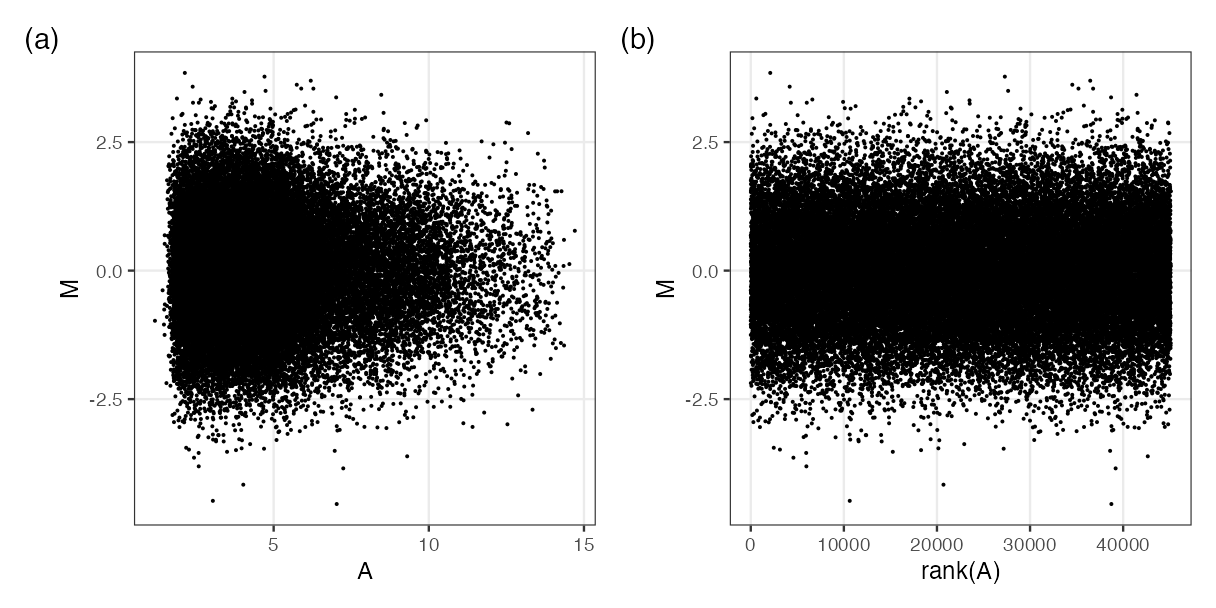
fig_3_43. Reproduces Holmes and Huber (2019), Figure 3.43. PDF · PNGDefinition 3.6 (MA plot)
For two log2 measurements \(x\) and \(y\) of the same features, the MA plot shows \(M=y-x\) (log fold change) against \(A=(x+y)/2\) (average log intensity). The map \((x,y)\mapsto(A,M)\) has matrix \(\begin{pmatrix}1/2&1/2\\-1&1\end{pmatrix}\) with determinant 1: a rotation by 45° combined with rescaling the two axes by \(1/\sqrt2\) and \(\sqrt2\), so area is preserved and the diagonal \(y=x\) becomes the horizontal line \(M=0\).
Filling the gap 3.17: why dense regions look more variable, and the rank transformation Section 3.11, Figure 3.43, Questions 3.9, 3.10
Derivation
Independence in the MA plot. \(\cov(A,M)=\cov(\tfrac{x+y}2,y-x)=\tfrac12(\var y-\var x)\). If the two measurements have equal variance this is zero, and for jointly normal \((x,y)\) \(A\) and \(M\) are then independent. For arrays 59 and 92, \(\operatorname{cor}(A,M)=-0.26\), because array 59 has the larger spread.
The artefact. The eye judges the spread of \(M\) at a given \(A\) by the extent of the cloud, i.e. by the most extreme points in a vertical strip. If the strip holds \(k\) independent \(\N(0,1)\) values, the expected maximum is \(\E\max=\int z\,k\phi(z)\Phi(z)^{k-1}\,\d z\), which grows like \(\sqrt{2\ln k}\): 2.51 for \(k=100\), 3.85 for \(k=10^4\) (computed numerically; the bound \(\sqrt{2\ln k}=4.29\) for \(k=10^4\) follows from the union bound with \(\Pr(Z>t)\le e^{-t^2/2}\)). A strip with 100 times more points therefore looks about 50% wider although the standard deviation is the same. In Figure 3.43(a) most probes have low \(A\), hence the funnel.
Ranks. Replacing \(A\) by \(\operatorname{rank}(A)\) maps the values (all distinct, or nearly) to \(1,\dots,n\): equally spaced, so every strip holds the same number of points, and the artefact disappears. \(\operatorname{rank}(A_i)/n=F_n(A_i)\) is the empirical version of the probability integral transform of Gap 3.8.
Question 3.9 (binning or densities?). Partly. Hexagon colours or density contours show the count per region, so the density of points is no longer confused with spread; but the outermost non-empty hexagons and the lowest contour still follow the extremes, which grow with the number of points. Running quantiles of \(M\) given \(A\) (for example the 5% and 95% quantiles in sliding windows of equal counts) show the conditional spread directly.
Question 3.10 (ranks for colour scales). Yes. Colour breaks at quantiles, breaks = quantile(z, seq(0, 1, length.out = 101)), give each of the 100 colours the same number of cells. Histogram equalisation in image processing does exactly this to grey levels: each intensity \(v\) is replaced by \(F_n(v)\), so the output histogram is approximately uniform and contrast is spent where the pixels are. The price is that equal colour steps no longer mean equal differences in value. ∎
3.12 Mathematical symbols and other fonts
Axis labels and annotations can contain mathematical notation through R's plotmath (?plotmath), written as R expressions: expression(nu), or frac(...), Gamma(...) and superscripts in a parsed string.
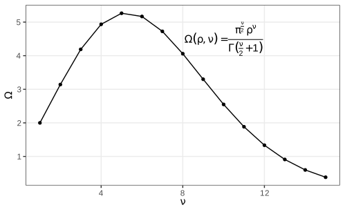
fig_3_44. Reproduces Holmes and Huber (2019), Figure 3.44. PDF · SVGFilling the gap 3.18: the volume of the unit ball Section 3.12, Figure 3.44
Result 3.8
The ball of radius \(\rho\) in \(\R^\nu\) has volume \(\Omega(\rho,\nu)=\pi^{\nu/2}\rho^\nu/\Gamma(\nu/2+1)\). For \(\rho=1\) it is largest at \(\nu=5\) (\(8\pi^2/15=5.264\)) and tends to 0 as \(\nu\to\infty\).
Proof
By scaling, \(\Omega(\rho,\nu)=\rho^\nu V_\nu\) with \(V_\nu=\Omega(1,\nu)\), so the shell between radii \(r\) and \(r+\d r\) has volume \(\nu V_\nu r^{\nu-1}\d r\). Compute \(I=\int_{\R^\nu}e^{-\|\mathbf x\|^2}\d\mathbf x\) two ways. As a product of one-dimensional integrals, \(I=(\int e^{-t^2}\d t)^\nu=\pi^{\nu/2}\). In shells, \(I=\int_0^\infty e^{-r^2}\nu V_\nu r^{\nu-1}\d r=\nu V_\nu\cdot\tfrac12\Gamma(\nu/2)=V_\nu\Gamma(\nu/2+1)\), substituting \(s=r^2\). Equate: \(V_\nu=\pi^{\nu/2}/\Gamma(\nu/2+1)\).
The ratio \(V_{\nu+2}/V_\nu=\pi/(\nu/2+1)=2\pi/(\nu+2)\) exceeds 1 exactly when \(\nu<2\pi-2\approx4.28\). So along the even dimensions \(V_2<V_4>V_6>\dots\) and along the odd ones \(V_1<V_3<V_5>V_7>\dots\); comparing the candidates, \(V_4=\pi^2/2=4.935\), \(V_5=8\pi^2/15=5.264\), \(V_6=\pi^3/6=5.168\), so the maximum is at \(\nu=5\). For \(\nu\ge5\) the ratio is at most \(2\pi/7<1\) and tends to 0, so \(V_\nu\to0\) faster than geometrically. A Monte Carlo estimate agrees for \(\nu=2,\dots,5\). ∎
Why it matters for data. The unit cube \([-1,1]^\nu\) has volume \(2^\nu\), so the fraction of it inside the inscribed ball, \(V_\nu/2^\nu\), is 0.52 for \(\nu=3\) and \(2.5\times10^{-8}\) for \(\nu=20\): in high dimensions almost all points are far from the centre and neighbourhoods are nearly empty, the reason for the slower rates of Gap 3.10.
Fonts are changed through the theme, theme(text = element_text(family = "Times")). Which families are available depends on the graphics device: the PDF device knows only the standard PostScript families unless others are registered (the extrafont package imports system fonts and registers them).
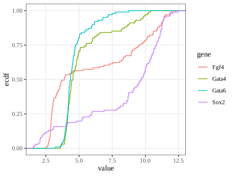
fig_3_45. Reproduces Holmes and Huber (2019), Figure 3.45. PDF · SVG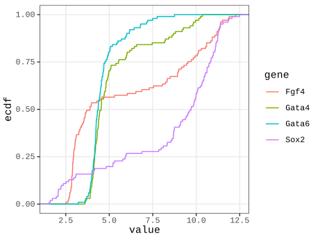
fig_3_46. Reproduces Holmes and Huber (2019), Figure 3.46. PDF · SVGTask (another font)
With extrafont: run font_import() once, then loadfonts() in each session, and use any name from fonts() in element_text(family = ...). Raster devices based on systemfonts (ragg) find installed system fonts directly, e.g. ragg::agg_png(...) with family = "Futura". (The book's task refers to Figure 3.45 where it means Figure 3.46.)
3.13 Genomic data
Genomic data come with coordinates on chromosomes, which organise everything else; displays must work at all scales from whole genomes to single bases. Genome browsers (the book's Figure 3.47 is a screenshot of one, not reproduced) show annotation tracks and read pile-ups. Programmatically, the book uses ggbio with example data from biovizBase: an ideogram of chromosome 1 and the locations of 500 RNA editing sites from the DARNED database (Holmes and Huber 2019, Section 3.13). ggbio does not work with the current ggplot2 4.x, so these figures are drawn directly with ggplot2 from the same data.
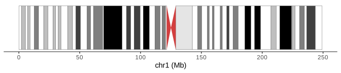
biovizBase::hg19IdeogramCyto. Code: fig_3_48. Reproduces Holmes and Huber (2019), Figure 3.48. PDF · SVG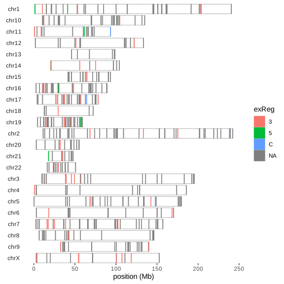
fig_3_49. Reproduces Holmes and Huber (2019), Figure 3.49. PDF · SVGQuestion 3.11 (ordering the chromosomes)
How can the order of the chromosomes in Figure 3.49 be fixed, and the missing chromosome lengths supplied?
Answer
Copy the hg19 lengths from biovizBase::ideoCyto$hg19 into the object, seqlengths(dn) = seqlengths(ideoCyto$hg19)[names(seqlengths(dn))], and set the order of the sequence levels with keepSeqlevels(dn, paste0("chr", c(1:22, "X"))), which also drops levels not listed. Figure 3.50 is the result.
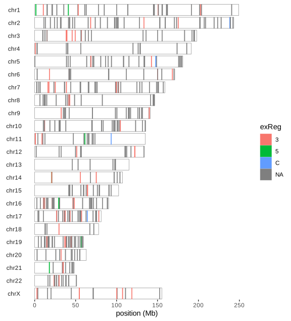
fig_3_50. Reproduces Holmes and Huber (2019), Figure 3.50. PDF · SVGQuestion 3.12 (what kind of object?)
What type of object is darned_hg19_subset500?
Answer
A GRanges object (GenomicRanges): one row per site with the required columns seqnames (chromosome), ranges (here intervals of width 1) and strand, plus metadata columns (mcols) such as the nucleotide change, gene, genic region (exReg) and source tissue, and a seqinfo with chromosome names and, after the fix, lengths. Its methods (overlaps, nearest features, coverage) make interval arithmetic on genomes safe and fast.
Summary
A graphic is data plus a statistic plus a mapping to visual properties, and the statistic deserves as much thought as the look. Bars of means hide distributions, and their error bars must be labelled (they are 95% t intervals in mean_cl_normal). Boxplots rest on sample quantiles and miss multimodality; kernel densities show it at the cost of a bandwidth, whose optimal size shrinks only like \(n^{-1/5}\); the ECDF needs no tuning, is unbiased, converges uniformly and has a distribution-free band. Transformations change densities and modes but not quantiles; variance-stabilising transformations come from the delta method. Overplotting is handled by transparency, binning or smoothing, each with its own blind spot, and dense regions look more variable than they are. Aspect ratio, colour space and ordering (of heatmap rows, of chromosomes) shape what the reader sees; choose them deliberately (Holmes and Huber 2019, Section 3.14).
Exercises
The six exercises of Chapter 3 (Holmes and Huber 2019, Section 3.16), restated in my own words. They are about software rather than mathematics; the solutions give working approaches and code written for these notes.
Exercise 3.1 (themes). Plot
mpgagainsthpfor themtcarsdata and comparetheme_bw()andtheme_minimal(). Which other themes exist, in ggplot2 and in the ggthemes package? Make a version in the style of The Economist with a smoothing line.Solution
ggplot2's complete themes are
theme_grey(the default),theme_bw,theme_linedraw,theme_light,theme_dark,theme_minimal,theme_classic,theme_voidandtheme_test. ggthemes adds many more, among themtheme_economist,theme_tufte,theme_few,theme_wsj,theme_fivethirtyeight,theme_excel,theme_solarizedandtheme_stata, each with matching colour scales. A theme changes only non-data elements; the data, geoms and statistics are untouched.library(ggplot2); library(ggthemes) ggcars <- ggplot(mtcars, aes(x = hp, y = mpg)) + geom_point() ggcars + geom_smooth(method = "loess", formula = y ~ x, colour = "#01a2d9") + theme_economist() + scale_colour_economist() + labs(x = "Gross horsepower", y = "Miles per US gallon")
The loess curve shows fuel consumption falling steeply up to about 150 hp and flattening above.
Exercise 3.2 (colour names and another palette). Find out which colour names base R accepts (
?colors, its examples and demo) and explore lists of R colour names. Redraw the heatmap of Figure 3.41 with a palette from the beyonce package.Solution
colors()returns the 657 names R accepts (white, the X11 names such asdarkorange3, and the grey/gray scales 0–100); any of them, a hex code"#RRGGBB"or"#RRGGBBAA", or a palette index can be given as a colour.col2rgb()converts names to RGB. The beyonce package is not on CRAN and is not installed here; its palettes are vectors of hex codes (beyonce_palette(k)), and any such vector can be used in the same way:pal <- colorRampPalette(beyonce::beyonce_palette(18))(100) # or any diverging set of colours pheatmap(m, color = pal, breaks = seq(-5, 5, length.out = 101), ...)
Since the heatmap shows fold changes around 0, the palette should be diverging with a light neutral colour in the middle (Gap 3.15);
colorspace::diverging_hcl(100, "Blue-Red 3")is such a palette with balanced luminance. A palette chosen for its look rather than its structure can make 0 look like an extreme.Exercise 3.3 (xkcd style). Make plots in the style of the xkcd webcomic, using the xkcd package and its vignette.
Solution
The xkcd package (not installed here) supplies
xkcdaxis()(hand-drawn looking axes),xkcdman()(stick figures) and instructions to install the xkcd font. The effect itself is easy to imitate: add small smooth random perturbations to lines and use a handwriting font, e.g.wobble <- function(x, s) x + s * stats::filter(rnorm(length(x)), rep(1/7, 7), circular = TRUE) d <- data.frame(x = seq(1, 55, length.out = 200)); d$y <- (d$x / 10)^4 ggplot(d, aes(wobble(x, 0.3), wobble(y, 4))) + geom_path(linewidth = 1.2) + theme_classic(base_family = "Comic Sans MS")
Such styling signals “sketch, not measurement” and is appropriate only where precision is not the point.
Exercise 3.4 (a shiny app). Write a shiny application that shows one of the chapter's plots with controls, for example to choose the genes in Figures 3.33–3.35.
Solution
library(shiny); library(ggplot2)
# dftx: cells in rows, probes as columns, with the cell annotation (Section 3.5)
probes <- c(Fn1 = "X1426642_at", Timd2 = "X1418765_at", Fgf4 = "X1420085_at",
            Gata4 = "X1418863_at", Gata6 = "X1425463_at", Sox2 = "X1416967_at")
ui <- fluidPage(
  selectInput("gx", "x gene", names(probes), "Fn1"),
  selectInput("gy", "y gene", names(probes), "Timd2"),
  radioButtons("facet", "facet by", c("none", "lineage", "Embryonic.day")),
  plotOutput("p"))
server <- function(input, output) {
  output$p <- renderPlot({
    p <- ggplot(dftx, aes(.data[[probes[input$gx]]], .data[[probes[input$gy]]])) +
      geom_point() + labs(x = input$gx, y = input$gy)
    if (input$facet != "none") p <- p + facet_wrap(vars(.data[[input$facet]]))
    p
  })
}
shinyApp(ui, server)
Each change of a control re-runs
renderPlotin the R session. The demonstrations of this course take the other route: the computation is reimplemented in JavaScript so the page runs without R.Exercise 3.5 (serialising graphics). How can a graphic be stored in a file for later use or for other software? How can interactive graphics be stored?
Solution
As drawings: vector formats (PDF, SVG, EPS) for line art and moderate numbers of points; raster formats (PNG, TIFF, JPEG for photographs only) at a stated resolution for dense plots and images (Section 3.4.2). As objects:
saveRDS(gg, "plot.rds")stores the ggplot object with its data, so it can be re-drawn and modified afterreadRDS, but only with compatible package versions. As code: the script plus the data is the most durable form. Interactive graphics: htmlwidgets such as plotly are saved as self-contained HTML (htmlwidgets::saveWidget(w, "plot.html", selfcontained = TRUE)) or as a JSON specification (plotly's JSON, Vega-Lite); rgl scenes withrglwidget()andsaveWidget. A shiny app needs a running R server and cannot be saved as a file of static content, unless it is compiled to run in the browser (shinylive, R through WebAssembly).Exercise 3.6 (simple, important graphics). Look at Figure 9 (page 82) of the European Medicines Agency's public assessment report on Comirnaty and at xkcd comic 2400.
Solution
The figure in the assessment report is a cumulative incidence plot of COVID-19 cases over time after the first dose, one curve per trial arm; the comic makes the point that some results need no test once they are drawn well. Cumulative incidence curves are close relatives of the ECDF (Section 3.6.7): one minus a Kaplan–Meier survival curve, which reduces to \(F_n\) when nothing is censored. What makes such a plot effective: one message, two curves, a shared time axis starting at the intervention, direct labels, and data shown as counts over time rather than as a single summary number.
Demonstrations for this chapter
Each demonstration runs in the browser on data exported by the R code, and its key numbers agree with R. The ▶ Demo boxes above open them already set to the case under discussion.
| Demonstration | What you can see | Sections |
|---|---|---|
| Kernel density estimation and the bandwidth | The four genes and a simulated mixture with known density; bandwidth slider, four kernels, Silverman, Scott and AMISE-optimal bandwidths, twenty replicates for bias and variance. Presets: 1 Fgf4 (Fig. 3.19); 2 undersmoothed; 3 oversmoothed; 4 bias and variance; 5 AMISE-optimal; 6 kernel shape. | 3.6.4–3.6.6 (Gaps 3.4, 3.5) |
| The empirical CDF, the DKW band and QQ plots | ECDFs of simulated samples and of the genes with the DKW band, the Kolmogorov–Smirnov distance, a coverage experiment and normal QQ plots. Presets: 1 70 normal draws (Fig. 3.23); 2 n = 5000; 3 band coverage; 4 Fgf4 (Fig. 3.24); 5 heavy tails; 6 right skew. | 3.6.2, 3.6.7 (Gaps 3.6–3.8) |
| 45,101 points on one plot | Two arrays as points with transparency, hexagonal bins and 2-D kernel densities; linear scale; MA and rank views. Presets: 1 all points (Fig. 3.27); 2 alpha 0.1 (Fig. 3.28); 3 2-D density (Fig. 3.30); 4 hexagons (Fig. 3.31); 5 linear scale; 6 rank view (Fig. 3.43). | 3.7, 3.11 (Gaps 3.10, 3.11, 3.17) |
| Variance-stabilising transformations | Standard deviation of transformed Poisson, negative binomial and microarray-type data against the mean: exact, delta method and simulation. Presets: 1 raw Poisson; 2 square root; 3 log(x + 1) for NB; 4 NB asinh; 5 log for microarray noise; 6 generalised log. | 3.11 (Gap 3.16), 3.6.8 |
The R code that produces every figure of this page is code/ch03_data_visualization.R (see the code index).
References
- Holmes, S. and Huber, W. (2019). Modern Statistics for Modern Biology. Cambridge University Press, Cambridge. Chapter 3.
- Anscombe, F. J. (1948). The transformation of Poisson, binomial and negative-binomial data. Biometrika, 35(3/4), 246–254. doi:10.1093/biomet/35.3-4.246.
- Bahadur, R. R. (1966). A note on quantiles in large samples. The Annals of Mathematical Statistics, 37(3), 577–580. doi:10.1214/aoms/1177699450.
- Carr, D. B., Littlefield, R. J., Nicholson, W. L. and Littlefield, J. S. (1987). Scatterplot matrix techniques for large N. Journal of the American Statistical Association, 82(398), 424–436.
- Cleveland, W. S. (1979). Robust locally weighted regression and smoothing scatterplots. Journal of the American Statistical Association, 74(368), 829–836. doi:10.1080/01621459.1979.10481038.
- Cleveland, W. S. and Devlin, S. J. (1988). Locally weighted regression: an approach to regression analysis by local fitting. Journal of the American Statistical Association, 83(403), 596–610. doi:10.1080/01621459.1988.10478639.
- Cleveland, W. S., McGill, M. E. and McGill, R. (1988). The shape parameter of a two-variable graph. Journal of the American Statistical Association, 83(402), 289–300.
- Durbin, B. P., Hardin, J. S., Hawkins, D. M. and Rocke, D. M. (2002). A variance-stabilizing transformation for gene-expression microarray data. Bioinformatics, 18(Suppl 1), S105–S110. doi:10.1093/bioinformatics/18.suppl_1.S105.
- Dvoretzky, A., Kiefer, J. and Wolfowitz, J. (1956). Asymptotic minimax character of the sample distribution function and of the classical multinomial estimator. The Annals of Mathematical Statistics, 27(3), 642–669. doi:10.1214/aoms/1177728174.
- Helmholtz, H. von (1867). Handbuch der physiologischen Optik. Voss, Leipzig.
- Huber, W., von Heydebreck, A., Sültmann, H., Poustka, A. and Vingron, M. (2002). Variance stabilization applied to microarray data calibration and to the quantification of differential expression. Bioinformatics, 18(Suppl 1), S96–S104. doi:10.1093/bioinformatics/18.suppl_1.S96.
- Ihaka, R. (2003). Colour for presentation graphics. In Proceedings of the 3rd International Workshop on Distributed Statistical Computing (DSC 2003), Vienna.
- Irizarry, R. A., Hobbs, B., Collin, F., Beazer-Barclay, Y. D., Antonellis, K. J., Scherf, U. and Speed, T. P. (2003). Exploration, normalization, and summaries of high density oligonucleotide array probe level data. Biostatistics, 4(2), 249–264. doi:10.1093/biostatistics/4.2.249.
- Lawrence, M. S. et al. (2013). Mutational heterogeneity in cancer and the search for new cancer-associated genes. Nature, 499, 214–218. doi:10.1038/nature12213.
- Massart, P. (1990). The tight constant in the Dvoretzky-Kiefer-Wolfowitz inequality. The Annals of Probability, 18(3), 1269–1283. doi:10.1214/aop/1176990746.
- McCormick, W. T., Schweitzer, P. J. and White, T. W. (1972). Problem decomposition and data reorganization by a clustering technique. Operations Research, 20(5), 993–1009. doi:10.1287/opre.20.5.993.
- Ohnishi, Y., Huber, W., Tsumura, A., Kang, M., Xenopoulos, P., Kurimoto, K., Oleś, A. K., Araúzo-Bravo, M. J., Saitou, M., Hadjantonakis, A.-K. and Hiiragi, T. (2014). Cell-to-cell expression variability followed by signal reinforcement progressively segregates early mouse lineages. Nature Cell Biology, 16(1), 27–37. doi:10.1038/ncb2881.
- Parzen, E. (1962). On estimation of a probability density function and mode. The Annals of Mathematical Statistics, 33(3), 1065–1076. doi:10.1214/aoms/1177704472.
- Rocke, D. M. and Durbin, B. (2001). A model for measurement error for gene expression arrays. Journal of Computational Biology, 8(6), 557–569.
- Rosenblatt, M. (1956). Remarks on some nonparametric estimates of a density function. The Annals of Mathematical Statistics, 27(3), 832–837. doi:10.1214/aoms/1177728190.
- Sheather, S. J. and Jones, M. C. (1991). A reliable data-based bandwidth selection method for kernel density estimation. Journal of the Royal Statistical Society: Series B, 53(3), 683–690. doi:10.1111/j.2517-6161.1991.tb01857.x.
- Silverman, B. W. (1986). Density Estimation for Statistics and Data Analysis. Chapman and Hall, London.
- Wickham, H. (2016). ggplot2: Elegant Graphics for Data Analysis, 2nd edition. Springer, New York.
- Wilkinson, L. (1999). Dot plots. The American Statistician, 53(3), 276–281.
- Wilkinson, L. (2005). The Grammar of Graphics, 2nd edition. Springer, New York.
- Zeileis, A., Hornik, K. and Murrell, P. (2009). Escaping RGBland: selecting colors for statistical graphics. Computational Statistics & Data Analysis, 53(9), 3259–3270. doi:10.1016/j.csda.2008.11.033.
The numerical statements in the text (the error-bar formula and coverage, the outlier probability, the kernel bias, variance and MISE formulas, the ECDF and DKW statements, the modes of array 64, the loess formulas, the kde2d convention, the hexagon counts, the banking ratio, the colour conversions, the dendrogram orderings, the transformation limits and the ball volumes) are computed by the course code.