Chapter 4. Mixture Models
Biological measurements are rarely drawn from one tidy textbook distribution: a population may consist of several subpopulations, a count may be zero for a structural reason or by chance, and the rate behind a count may itself vary from sample to sample. Mixture models describe all of these situations by a two-level generating process: first draw a hidden label or parameter, then draw the observation given it. These notes follow Holmes and Huber (2019), Modern Statistics for Modern Biology, Chapter 4, and add the mathematics the book states without proof: the EM algorithm and why it never decreases the likelihood, the zero-inflated Poisson, the bootstrap and why it works, the Laplace and gamma-Poisson distributions as infinite mixtures, and variance-stabilising transformations from the delta method.
Ch. 1 Discrete data Ch. 2 Statistical modeling Ch. 3 Data visualization Ch. 4 Mixture models Ch. 5 Clustering Ch. 6 Testing Ch. 7 Multivariate analysis Ch. 8 Count data and GLMs Ch. 9 Heterogeneous data Ch. 10 Networks and trees Ch. 11 Image data Ch. 12 Supervised learning Ch. 13 Experimental design
How to read these notes
They follow the book. Sections carry the book's numbers (4.2, 4.2.2, ...) and displayed equations that appear in the book carry its equation numbers, e.g. (4.5); equations without a number are steps the book skips. Book figures are reproduced from scratch by the course's R code and keep their book numbers.
Filling the gaps. The book is written for biologists and states many results without derivation. Wherever it does, an orange Filling the gap box gives the full argument at the level of a graduate statistics course: assumptions, every step, and a numerical confirmation. Proofs start hidden; open one with its bar, or use the button below.
Questions and corrections. The book's in-text questions appear as grey Question boxes with worked answers; red Correction boxes flag places where the book's text, equations or code are wrong, with the evidence. The ▶ Demo boxes open an interactive demonstration already set to the case under discussion.
Main reference
S. Holmes and W. Huber, Modern Statistics for Modern Biology, Cambridge University Press (2019), Chapter 4 "Mixture Models". Section, equation, figure, question and exercise numbers below refer to this book. Further reading is listed in the references.
The explanations, derivations and code are my own; results are cited by their numbers in the book.
The chapter at a glance
- 4.2 A finite mixture \(f=\sum_k\pi_kf_k\) is the distribution of \(X\) when a hidden label \(U\) picks the component. Its moments follow from the laws of total expectation and variance; a two-component normal mixture with equal weights and variances is bimodal exactly when the means are more than two standard deviations apart (Result 4.1). Parameters are identified only up to relabelling (Result 4.2). The likelihood has no closed-form maximiser, is unbounded, and has saddle points; the EM algorithm alternates posterior membership weights (E step) and weighted maximum likelihood (M step), and never decreases the likelihood (Result 4.3). Zero inflation is a mixture with a point mass at zero, fitted by EM as well (Result 4.4).
- 4.3 The empirical distribution \(\hat F_n\) puts mass \(1/n\) on each observation and converges uniformly to \(F\) (Result 4.5). The bootstrap estimates the sampling distribution of a statistic by the distribution it has when the data are drawn from \(\hat F_n\); for the mean and the median this is known exactly (Result 4.6), and for smooth statistics it is consistent (Result 4.7).
- 4.4 Mixing over a continuous parameter builds new distributions: an exponential mixture of normal variances is the Laplace distribution and, with a drift, the asymmetric Laplace (Results 4.8, 4.9); a gamma mixture of Poisson rates is the negative binomial, with variance \(\mu+\mu^2/a\) (Result 4.10). When the variance is a function \(v(\mu)\) of the mean, the delta method gives the variance-stabilising transformation \(g'=1/\sqrt{v}\): the square root for Poisson counts, the logarithm for a constant coefficient of variation and \(\asinh(\sqrt{\alpha x})/\sqrt\alpha\) for gamma-Poisson counts (Result 4.11).
Notation. \(\phi(x\given\mu,\sigma^2)\) is the normal density with mean \(\mu\) and variance \(\sigma^2\) (the book writes \(N(\mu,\sigma)\) in places, with \(\sigma\) the standard deviation; here the second argument is always a variance). \(\Pois(\lambda)\), \(\Exp(\lambda)\) (rate \(\lambda\), mean \(1/\lambda\)), \(\Gam(a,b)\) (shape \(a\), rate \(b\)), \(\NB(\mu,a)\) (mean \(\mu\), size \(a\)) and \(\Bin(n,p)\) are the usual families. \(\ind\{A\}\) is the indicator of the event \(A\). Data are \(x_1,\dots,x_n\), independent and identically distributed unless said otherwise.
Prerequisites. Maximum likelihood, the binomial and Poisson distributions and the chi-square goodness of fit (book Chapters 1 and 2), the empirical cumulative distribution function (book Section 3.6.7), conditional expectation and Jensen's inequality.
4.2 Finite mixtures
A finite mixture describes a population made of a few subpopulations, each with its own distribution, when we cannot see which subpopulation an observation came from. The book's opening example is the bimodal histogram of CpG-island scores of its Chapter 2; this chapter builds such distributions by simulation, then asks how to recover the components from data alone.
Definition 4.1 (finite mixture, latent label) Section 4.2, (4.1)–(4.3)
Let \(f_1,\dots,f_K\) be probability densities (or probability mass functions) and let \(\pi_1,\dots,\pi_K\ge0\) with \(\sum_k\pi_k=1\). The finite mixture with mixing proportions \(\pi_k\) and components \(f_k\) has density
\[ f(x)=\sum_{k=1}^K\pi_k f_k(x). \]Equivalently, \(X\) is generated in two steps: draw a latent label \(U\in\{1,\dots,K\}\) with \(\Pr(U=k)=\pi_k\), then draw \(X\) from \(f_U\). The book's two-component normal mixture (4.3) is the case \(K=2\), \(\pi_1=\lambda\), \(f_k=\phi(\cdot\given\mu_k,\sigma_k^2)\), with parameter vector \(\theta=(\lambda,\mu_1,\mu_2,\sigma_1,\sigma_2)\).
4.2.1 Simple examples and computer experiments
The first experiment flips a fair coin and draws from \(\N(1,0.5^2)\) on heads and from \(\N(3,0.5^2)\) on tails, 10,000 times. With one million draws and 200 bins the histogram becomes indistinguishable from a smooth curve, the mixture density (4.1).
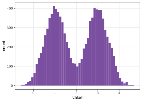
fig_4_1. Reproduces Holmes and Huber (2019), Figure 4.1. Download: PDF · SVG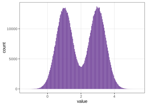
fig_4_2. Reproduces Holmes and Huber (2019), Figure 4.2. Download: PDF · SVGQuestions 4.1 and 4.2 (vectorised simulation)
Generate the mixture without an explicit loop over coin flips, then with one million flips and 200 bins.
Answer
Draw all coin flips at once and pass vectors of means and standard deviations to rnorm: x <- rnorm(n, mean = ifelse(coin, 1, 3), sd = 0.5), which is what sim_fair() in the course code does. Each bin count of the histogram is binomial with mean \(n\int_{\text{bin}}f\), so the relative noise of a bin is about \(1/\sqrt{\text{count}}\); with \(10^6\) draws the bins hold thousands of values and the histogram traces the density to within a few per cent (Figure 4.2).
The density of one component alone, here \(\N(1,0.5^2)\), is the normal density
\[ \phi(x\given\mu,\sigma^2)=\frac{1}{\sigma\sqrt{2\pi}}\exp\Big\{-\frac12\Big(\frac{x-\mu}{\sigma}\Big)^2\Big\}, \]and the histogram of the heads draws, scaled to unit area, follows it (Figure 4.3, Question 4.3). Adding the two weighted component densities gives the mixture density
\[ f(x)=\tfrac12\phi(x\given1,0.25)+\tfrac12\phi(x\given3,0.25). \tag{4.1} \]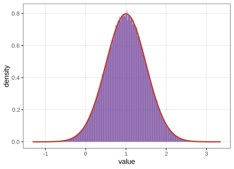
fig_4_3. Reproduces Holmes and Huber (2019), Figure 4.3. Download: PDF · SVG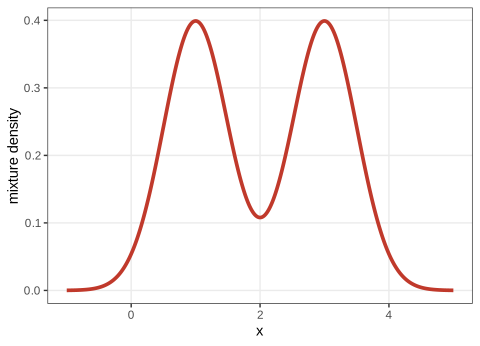
fig_4_4. Reproduces Holmes and Huber (2019), Figure 4.4. Download: PDF · SVGFilling the gap 4.1: why a mixture is the distribution of the two-step experiment Section 4.2.1, (4.1)
The book says that the limiting curve of the histograms "is" the sum of the two weighted densities. Let \(U\) be the coin (\(U=1\) heads with probability \(\lambda\)) and \(X\given U=k\sim f_k\). For any interval \(A\), the law of total probability gives
\[ \Pr(X\in A)=\sum_{k}\Pr(U=k)\Pr(X\in A\given U=k)=\int_A\big\{\lambda f_1(x)+(1-\lambda)f_2(x)\big\}\,\d x, \]so \(\lambda f_1+(1-\lambda)f_2\) is a density of \(X\) (it is non-negative and integrates to \(\lambda+(1-\lambda)=1\)). The histogram with bin width \(h\) estimates \(\Pr(X\in\text{bin})/h\), which tends to \(f(x)\) as \(n\to\infty\) and then \(h\to0\) (the strong law of large numbers for the bin frequency, then the fundamental theorem of calculus for continuous \(f\)). The same argument with \(K\) components gives Definition 4.1.
The joint density of the label and the observation is \(p(x,u)=\pi_uf_u(x)\), the book's (4.2); summing it over \(u\) gives the mixture, and dividing by the sum gives the posterior label probabilities used by EM in Section 4.2.2.
Result 4.1 (moments and modes of a mixture) Section 4.2.1, Figures 4.4 and 4.5
(a) If component \(k\) has mean \(\mu_k\) and variance \(\sigma_k^2\), the mixture has mean and variance
\[ \E X=\sum_k\pi_k\mu_k=:\bar\mu,\qquad \var X=\sum_k\pi_k\sigma_k^2+\sum_k\pi_k(\mu_k-\bar\mu)^2 . \]The variance of a mixture is the average within-component variance plus the variance of the component means; mixing always adds spread.
(b) The equal-weight mixture \(\tfrac12\phi(x\given\mu_1,\sigma^2)\)
Proof
(a) By the law of total expectation \(\E X=\E\{\E(X\given U)\}\)
(b) Shift and scale so that \(\sigma=1\) and the means are \(\pm\delta\), \(\delta=|\mu_1-\mu_2|/(2\sigma)\). Then \(f(x)\propto e^{-(x-\delta)^2/2}\)
For \(x\ge\delta\) both terms are negative, so all critical points with \(x>0\) lie in \((0,\delta)\). There, \(f'(x)=0\) is equivalent to \((\delta-x)/(\delta\)
Now \(h(0)=0\), \(h'(0)=1-\delta^2\), \(h\) is convex on \([0,1)\) (because \(\operatorname{artanh}''(t)\)
The book's two examples. In Figure 4.4 the means are 2 apart and \(2\sigma=1\): bimodal. In Figure 4.5 the means 1 and 2 are 1 apart and \(2\sigma=2\sqrt{0.5}=1.41\): the density has a single mode, which is why that mixture is "harder to recognize". Numerically, the threshold is confirmed (1 mode at separation 1.9 and 2.0, 2 modes at 2.1).
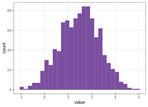
fig_4_5. Reproduces Holmes and Huber (2019), Figure 4.5. Download: PDF · SVGQuestions 4.4 and 4.5 (the hidden mixture of Figure 4.5)
Guess the two means of Figure 4.5 by simulation; then explain why the stacked bars of Figure 4.7, but not the overlaid ones of Figure 4.6, add up to the bars of Figure 4.5.
Answer
The data were drawn as a fair mixture of \(\N(1,0.5)\) and \(\N(2,0.5)\) (variance 0.5). Trial simulation finds the location (the overall mean \(1.5\)) easily but hardly the separation, because by Result 4.1(b) the density is unimodal and its shape changes only slowly with the separation. In Figure 4.6 each bar of one colour is drawn from zero, so where both components contribute the shorter bar is hidden behind the taller one; stacking (Figure 4.7) places one count on top of the other, so the total height is the count of the bin in Figure 4.5.
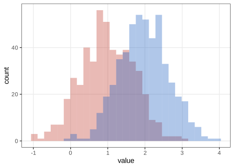
fig_4_6. Reproduces Holmes and Huber (2019), Figure 4.6. Download: PDF · SVG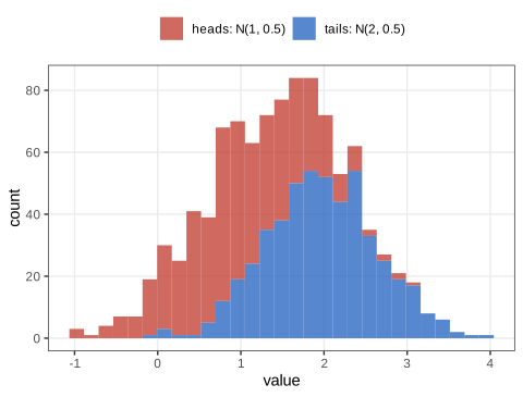
fig_4_7. Reproduces Holmes and Huber (2019), Figure 4.7. Download: PDF · SVGThe coin flips told us which component each value came from. In real data that information is missing, and the next section is about recovering it.
Result 4.2 (identifiability of finite normal mixtures) Section 4.2.2; Exercise 4.4
A parametric family \(\{f_\theta\}\) is identifiable if \(f_\theta=f_{\theta'}\) implies \(\theta=\theta'\). A mixture family can at best be identifiable up to relabelling: permuting the components (\(\lambda\leftrightarrow1-\lambda\), \(\mu_1\leftrightarrow\mu_2\), \(\sigma_1\leftrightarrow\sigma_2\)) leaves the density unchanged ("label switching"). Finite mixtures of normal distributions are identifiable in this sense (Teicher 1963): if \(\sum_{k=1}^K\pi_k\phi(\cdot\given\mu_k,\sigma_k^2)\)
Proof (the tail argument)
Suppose the two mixtures agree but their sets of triples differ; cancel the common triples, so that, after moving terms to one side, \(\sum_j c_j\phi(x\given m_j,s_j^2)\)
Where identifiability fails. Mixtures of Bernoulli distributions are not identifiable: \(\lambda\,\mathrm{Bern}(p_1)\)
4.2.2 Discovering the hidden class labels
Augment each observation \(x_i\) by its unobserved label \(u_i\). The joint density factorises as
\[ p(x,u\given\theta)=p(x\given u,\theta)\,p(u\given\theta), \tag{4.2} \]and the two-component normal mixture with unequal weights is
\[ f(x)=\lambda\phi_1(x)+(1-\lambda)\phi_2(x),\qquad \phi_k(x)=\phi(x\given\mu_k,\sigma_k^2),\quad \lambda\in[0,1]. \tag{4.3} \]If the labels were known, the complete-data likelihood would factorise over the two groups:
\[ p(x,u\given\theta)=\prod_{i:\,u_i=1}\lambda\phi_1(x_i)\times\prod_{i:\,u_i=2}(1-\lambda)\phi_2(x_i). \tag{4.4} \](The book's (4.4) omits the factors \(\lambda\) and \(1-\lambda\); they are needed for the estimate of \(\lambda\) and appear in the version above.)
Filling the gap 4.2: maximum likelihood with known labels Section 4.2.2, (4.4)
Let \(n_k=\#\{i:u_i=k\}\). The log of (4.4) is
\[ \ell_c(\theta)=n_1\log\lambda+n_2\log(1-\lambda)+\sum_{i:u_i=1}\log\phi_1(x_i)+\sum_{i:u_i=2}\log\phi_2(x_i), \]a sum of three terms that depend on disjoint parameter blocks, so each is maximised separately. (i) \(\partial/\partial\lambda\): \(n_1/\lambda-n_2/(1-\lambda)=0\) gives \(\hat\lambda=n_1/n\), and the second derivative \(-n_1/\lambda^2\)
The Hessian in \((\mu_k,\sigma_k^2)\) at this point is \(\operatorname{diag}(-n_k/\hat\sigma_k^2,\,-n_k/(2\hat\sigma_k^4))\), negative definite, and the log-likelihood tends to \(-\infty\) at the boundary (\(\sigma_k^2\to0\) or \(\infty\), \(|\mu_k|\to\infty\)) as long as group \(k\) has two distinct values, so this is the global maximum. The book's code uses sd(), which divides by \(n_k-1\) (the unbiased variance); the maximum-likelihood estimate divides by \(n_k\). The difference is a factor \(\sqrt{n_k/(n_k-1)}\), about 1% for the book's groups of about 50.
Question 4.6 (why no closed form when the labels are hidden)
With \(\lambda=\tfrac12\) known but the labels hidden, write the log-likelihood. What prevents an explicit maximum-likelihood solution?
Answer
The observed-data log-likelihood is \(\ell(\theta)\)
Replacing the hard labels by membership weights, the posterior probability that an observation with value \(x\) came from component 1 is
\[ w(x,1)=\frac{\lambda\phi_1(x)}{\lambda\phi_1(x)+(1-\lambda)\phi_2(x)},\qquad w(x,2)=1-w(x,1), \tag{4.5} \]which is Bayes' theorem applied to the joint density (4.2): the prior \(\Pr(U=1)=\lambda\) becomes the posterior \(\Pr(U=1\given X=x)\). The algorithm alternates an E step (compute the weights at the current parameters) and an M step (re-estimate the parameters by weighted maximum likelihood).
Filling the gap 4.3: the marginal likelihood, correctly Section 4.2.2, (4.6), (4.7)
The quantity to maximise is the likelihood of what was observed, the marginal (or observed-data) likelihood, obtained by summing the joint density over the unobserved labels:
\[ L_\text{marg}(\theta;x)=\sum_{u_1,\dots,u_n}\prod_{i=1}^np(x_i,u_i\given\theta)=\prod_{i=1}^n\sum_{u=1}^2p(x_i,u\given\theta)=\prod_{i=1}^n\big\{\lambda\phi_1(x_i)+(1-\lambda)\phi_2(x_i)\big\}. \tag{4.6} \]The middle equality interchanges the sum over the \(2^n\) label configurations with the product, which is allowed because the labels are independent across observations (expand the product of sums). The book's (4.7) multiplies each term by the membership weight, \(\prod_i\sum_up(x_i,u\given\theta)\,w(x_i,u\given\theta)\); that is not the marginal likelihood (it double-counts the label probabilities). On the Exercise 4.1 data at the EM solution, the correct log-likelihood is 417.22 while the printed formula gives 91.78. The marginal likelihood is not "intractable": it is cheap to evaluate. What has no closed form is its maximiser.
Filling the gap 4.4: the shape of the mixture likelihood Section 4.2.2, Question 4.6
Score equations. Write \(w_i=w(x_i,1)\). Differentiating \(\ell(\theta)=\sum_i\log f(x_i)\) and using \(\partial\phi_1/\partial\mu_1\)
and similarly for \(\sigma_1^2\), \(\mu_2\), \(\sigma_2^2\). Setting them to zero says that \(\hat\theta\) reproduces itself through weighted means and variances with weights computed at \(\hat\theta\): the stationary points of \(\ell\) are exactly the fixed points of the EM map below.
The likelihood is unbounded. Put \(\mu_1=x_1\) and let \(\sigma_1\to0\) with the other parameters fixed and \(0<\lambda<1\). The term for \(x_1\) is at least \(\lambda/(\sigma_1\sqrt{2\pi})\)
Saddle points. If both components start identical (\(\mu_1=\mu_2\), \(\sigma_1=\sigma_2\)), every weight equals \(\lambda\), the weighted means and variances of the two components are equal, and the M step returns two identical components again. This is a stationary point of \(\ell\) (a one-component fit), not a maximum: on the Exercise 4.1 data it sits at log-likelihood 312.6 against 417.2 at the two-component solution. Local maxima also occur (Question 4.7); hence the book's advice to run EM from several starting points.
This alternation is a special case of a general algorithm. With observed data \(x\), latent data \(u\) and a parameter \(\theta\), define the expected complete-data log-likelihood
\[ Q(\theta,\theta_t)=\int\log p(x,u\given\theta)\,p(u\given x,\theta_t)\,\d u, \tag{4.8} \]a sum over \(u\) when the latent variable is discrete. The E step computes the conditional distribution \(p(u\given x,\theta_t)\), and with it the function \(Q(\cdot,\theta_t)\); the M step sets
\[ \theta_{t+1}=\argmax_\theta Q(\theta,\theta_t). \tag{4.9} \]This is the EM algorithm of Dempster, Laird and Rubin (1977).
Filling the gap 4.5: \(Q\) for a normal mixture Section 4.2.2, (4.8)
Take \(K\) components, \(\theta=(\pi_k,\mu_k,\sigma_k^2)_{k\le K}\). Code the label of observation \(i\) by indicators \(z_{ik}=\ind\{u_i=k\}\). The complete-data log-likelihood is linear in the indicators:
\[ \log p(x,u\given\theta)=\sum_{i=1}^n\sum_{k=1}^Kz_{ik}\big\{\log\pi_k+\log\phi(x_i\given\mu_k,\sigma_k^2)\big\}. \]Given \(x\) and \(\theta_t\), the labels are independent with \(\Pr(u_i=k\given x,\theta_t)=r_{ik}\), where
\[ r_{ik}=\frac{\pi_k^{(t)}\phi(x_i\given\mu_k^{(t)},\sigma_k^{2(t)})}{\sum_{j}\pi_j^{(t)}\phi(x_i\given\mu_j^{(t)},\sigma_j^{2(t)})} \](Bayes' theorem; for \(K=2\) this is (4.5)). Since \(\E(z_{ik}\given x,\theta_t)=r_{ik}\) and the log-likelihood is linear in \(z_{ik}\),
\[ Q(\theta,\theta_t)=\sum_{i}\sum_{k}r_{ik}\big\{\log\pi_k+\log\phi(x_i\given\mu_k,\sigma_k^2)\big\}. \]So the E step amounts to computing the \(n\times K\) matrix of responsibilities \(r_{ik}\); \(Q\) is then the complete-data log-likelihood with the unknown indicators replaced by them.
Filling the gap 4.6: the M step in closed form Section 4.2.2, (4.9); Exercise 4.1
Let \(N_k=\sum_ir_{ik}\) (the "soft count" of component \(k\); \(\sum_kN_k=n\)). \(Q\) separates into a part for the weights and a part for each component.
Weights. Maximise \(\sum_kN_k\log\pi_k\) subject to \(\sum_k\pi_k=1\). With a Lagrange multiplier \(\nu\), \(N_k/\pi_k=\nu\) for all \(k\); summing \(\pi_k=N_k/\nu\) over \(k\) gives \(\nu=n\). The objective is strictly concave on the simplex (a positive combination of concave logs), so the stationary point is the maximum:
\[ \pi_k^{(t+1)}=\frac{N_k}{n}=\frac1n\sum_ir_{ik}. \]Means and variances. For component \(k\), \(\sum_ir_{ik}\log\phi(x_i\given\mu_k,\sigma_k^2)\)
with negative definite Hessian \(\operatorname{diag}(-N_k/\sigma_k^2,-N_k/(2\sigma_k^4))\) at the solution. These are R's weighted.mean and the weighted variance with weights \(r_{ik}\), exactly the five lines of the M step in the book's Exercise 4.1 code. (A numerical maximiser of \(Q\) gives the same values to \(10^{-7}\).) With a common variance \(\sigma^2\) for all components, the variance update becomes \(\sum_i\sum_kr_{ik}(x_i-\mu_k)^2/n\).
Algorithm 4.1 (EM for a mixture of \(K\) normals) Section 4.2.2; Exercise 4.1
- Start from parameters \(\theta_0\) (for example equal weights, means at sample quantiles, all variances equal to the sample variance), or from random responsibilities followed by an M step (the book's choice).
- E step. Compute \(r_{ik}\) at \(\theta_t\) and the log-likelihood \(\ell(\theta_t)\)
\({}=\sum_i\log\sum_k\pi_k^{(t)}\phi(x_i\given\mu_k^{(t)},\sigma_k^{2(t)})\) (on the log scale with the log-sum-exp device of Filling the gap 4.19). - M step. Update \(\pi_k,\mu_k,\sigma_k^2\) by Filling the gap 4.6.
- Stop when \(|\ell(\theta_{t+1})\)
\({}-\ell(\theta_t)|\) falls below a tolerance (after a minimum and before a maximum number of iterations); otherwise go to 2. - Repeat from several starts and keep the solution with the largest log-likelihood, avoiding degenerate solutions with a vanishing variance.
Result 4.3 (EM never decreases the likelihood) Section 4.2.2
Let \(\ell(\theta)=\log p(x\given\theta)\) be the observed-data log-likelihood and let \(\theta_{t+1}\) satisfy \(Q(\theta_{t+1},\theta_t)\)
Proof (Jensen's inequality)
For every \(u\) with \(p(u\given x,\theta)>0\), \(p(x\given\theta)\)
(This identity holds for every \(\theta\); it holds to \(10^{-12}\) on the Exercise 4.1 data.) Now
\[ H(\theta,\theta_t)-H(\theta_t,\theta_t)=\int\log\frac{p(u\given x,\theta_t)}{p(u\given x,\theta)}\,p(u\given x,\theta_t)\,\d u=\KL\big(p(\cdot\given x,\theta_t)\,\big\|\,p(\cdot\given x,\theta)\big)\ge0, \]because by Jensen's inequality for the concave logarithm, \(-\KL=\E_t\log\frac{p_\theta}{p_t}\)
Equality forces both brackets to vanish, which gives the equality statement. ∎
What this does and does not give. A non-decreasing sequence \(\ell(\theta_t)\) that is bounded above converges. Under continuity conditions (Wu 1983), every limit point of \(\theta_t\) is a stationary point of \(\ell\): a local maximum, or occasionally a saddle point such as the identical-components start. Since the normal-mixture likelihood is unbounded, the sequence can also run off to a degenerate solution with \(\sigma_k\to0\); in practice this happens for components that capture one or two points. Equivalently, EM is coordinate ascent on the lower bound \(\ell(\theta)\)
Filling the gap 4.7: how fast EM converges Section 4.2.2; Exercise 4.1
Near a strict local maximum \(\hat\theta\), the EM map \(M(\theta)\) (one E step and one M step) is differentiable with \(M(\hat\theta)=\hat\theta\), so \(\theta_{t+1}\)
where \(I_c=-\partial^2Q(\theta,\hat\theta)/\partial\theta\partial\theta^\T\) is the complete-data information, \(I_o=-\partial^2\ell/\partial\theta\partial\theta^\T\) the observed information and \(I_m=I_c-I_o\) the "missing" information (Dempster, Laird and Rubin 1977). Convergence is linear, with rate the largest eigenvalue of \(J\), the largest fraction of information lost by not seeing the labels. Well-separated components (labels nearly known) converge fast; overlapping components converge very slowly. In the course runs, the log-likelihood increments shrink by a factor of about 0.947 per iteration on the Exercise 4.1 data (422 iterations to a change below \(10^{-12}\)) and by about 0.998 per iteration on the overlapping mixture of Figure 4.5, which had not met the same tolerance after 5,000 iterations.
Question 4.7 (comparing EM implementations)
Run an EM implementation from several starting values on a sample of 100 \(\N(-0.2,0.5^2)\) and 50 \(\N(0.5,1)\) values, and compare with mixtools::normalmixEM.
Answer
Our own EM (em_mix2) and normalmixEM agree to \(2\times10^{-7}\) on the Exercise 4.1 data from the same start. On the Question 4.7 sample (course seed) the quartile start converges to \(\hat\lambda=0.927\), \(\hat\mu=(-0.101,1.941)\), \(\hat\sigma=(0.587,0.881)\), log-likelihood \(-164.29\), while the true parameters give \(-166.91\): the maximum-likelihood fit explains most of the data by one broad component and a handful of large values by a second one, far from the generating mixture. With 150 points and overlapping components the likelihood is flat and multimodal, the book's run lands elsewhere (0.870, 0.130, \(-0.238\), 1.473, ...), and different starts give different local maxima. This is the practical face of Filling the gap 4.7: weak information about the labels means a flat likelihood.
EM teaches three ideas the book stresses: soft assignment (each observation contributes to every component with weight \(r_{ik}\)), alternating between two easy problems instead of solving one hard one, and averaging over hidden variables rather than fixing them. The same scheme reappears in hidden Markov models, factor analysis, missing-data problems and the zero-inflated models below.
4.2.3 Models for zero inflated data
Counts of a species at a site, or of reads in a genomic bin, are often zero for two different reasons: the thing counted is absent (a structural zero), or it is present but the random sample happened to contain none (a sampling zero).
Definition 4.2 (zero-inflated distribution) Section 4.2.3, (4.10)
Given a count distribution \(f_\text{count}\) on \(\{0,1,2,\dots\}\) and \(\pi\in[0,1)\), the zero-inflated distribution is the mixture of a point mass at zero and \(f_\text{count}\):
\[ f_\text{zi}(x)=\pi\,\delta_0(x)+(1-\pi)\,f_\text{count}(x),\qquad \delta_0(x)=\ind\{x=0\}. \tag{4.10} \]With \(f_\text{count}=\Pois(\lambda)\) it is the zero-inflated Poisson \(\mathrm{ZIP}(\pi,\lambda)\) (Lambert 1992); with a negative binomial it is the zero-inflated negative binomial (ZINB). For counts, "Dirac's delta function" of the book is simply the probability mass function of the constant 0.
Result 4.4 (zero-inflated Poisson) Section 4.2.3
If \(X\sim\mathrm{ZIP}(\pi,\lambda)\) then \(\Pr(X=0)=\pi+(1-\pi)e^{-\lambda}\), \(\Pr(X=k)=(1-\pi)e^{-\lambda}\lambda^k/k!\) for \(k\ge1\),
\[ \E X=(1-\pi)\lambda,\qquad \var X=(1-\pi)\lambda(1+\pi\lambda), \]so \(\var X>\E X\) when \(\pi>0\): zero inflation produces overdispersion. For data with \(n_0\) zeros among \(n\) and mean \(\bar x\), the maximum-likelihood estimates (when \(n_0/n>e^{-\bar x}\), i.e. when there are more zeros than a Poisson with the same mean would give) solve
\[ (1-\hat\pi)\hat\lambda=\bar x,\qquad \hat\pi+(1-\hat\pi)e^{-\hat\lambda}=\frac{n_0}{n}: \]the fit reproduces the sample mean and the observed fraction of zeros exactly. Eliminating \(\hat\pi\), \(\hat\lambda\) is the unique positive root of \(\hat\lambda(1\)
Proof
Moments. Write \(X=(1-B)Y\) with \(B\sim\mathrm{Bern}(\pi)\) independent of \(Y\sim\Pois(\lambda)\). Then \(\E X=(1-\pi)\lambda\) and \(\E X^2=(1-\pi)(\lambda+\lambda^2)\), so \(\var X=(1-\pi)(\lambda\)
Likelihood equations. With \(p_0=\pi+(1-\pi)e^{-\lambda}\) and \(S=\sum_ix_i\), the log-likelihood is \(\ell=n_0\log p_0\)
The first equation gives \(n_0(1-\pi)(1\)
Filling the gap 4.8: EM for the zero-inflated Poisson Section 4.2.3
The latent variable is the indicator \(Z_i=1\) if observation \(i\) is a structural zero. Only zeros can be structural, so for \(x_i>0\), \(Z_i=0\) with certainty, and for \(x_i=0\) Bayes' theorem gives
\[ \tau=\Pr(Z_i=1\given X_i=0)=\frac{\pi}{\pi+(1-\pi)e^{-\lambda}} . \]The complete-data log-likelihood is \(\sum_i\{Z_i\log\pi\)
which is maximised in closed form: \(\pi'=n_0\tau/n\) (the expected fraction of structural zeros) and \(\lambda'=S/(n-n_0\tau)\) (the total count divided by the expected number of non-structural observations). By Result 4.3 each iteration increases the likelihood, and the fixed point satisfies the likelihood equations of Result 4.4.
The ChIP-Seq data. The 256,523 bins of 200 nucleotides on chromosome 22 (STAT1 ChIP in GM12878) have mean \(\bar x=1.803\) tag counts and 111,679 zeros (43.5%), while a Poisson with that mean predicts \(e^{-1.803}=16.5\%\) zeros (42,281 bins). EM from \(\pi=0.5\), \(\lambda=\bar x\) converges in 14 iterations to \(\hat\pi=0.4070\), \(\hat\lambda=3.040\) (identical to a direct numerical maximisation). Note that \(\hat\pi\) is smaller than the raw fraction of zeros 0.435: part of the zeros are sampling zeros of the Poisson component.
Algorithm 4.2 (EM for a zero-inflated count model) Section 4.2.3
- Start from \(\pi_0\in(0,1)\) and count-model parameters \(\eta_0\) (for the Poisson, \(\lambda_0=\bar x\)).
- E step. \(\tau=\pi/\{\pi\)
\({}+(1-\pi)f_\text{count}(0\given\eta)\}\), the posterior probability that a zero is structural. - M step. \(\pi\leftarrow n_0\tau/n\); fit \(f_\text{count}\) by weighted maximum likelihood with weight \(1-\tau\) on every zero and 1 on every non-zero count. (Poisson: \(\lambda=S/(n-n_0\tau)\). Negative binomial: the weighted mean for \(\mu\), then a one-dimensional search for the size.)
- Repeat until the log-likelihood changes by less than a tolerance.
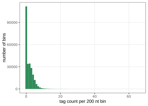
fig_4_8. Reproduces Holmes and Huber (2019), Figure 4.8. Download: PDF · SVGQuestion 4.8 (log scale, and the proportion of zeros)
Redraw the histogram with a logarithmic count axis and estimate \(\pi_0\), the proportion of bins with zero counts.
Answer
Figure 4.9. The empirical proportion of zero bins is \(\hat\pi_0=111{,}679/256{,}523\)
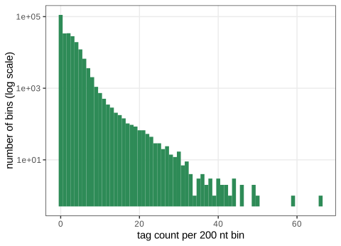
fig_4_9. Reproduces Holmes and Huber (2019), Figure 4.9. Download: PDF · SVG4.2.4 More than two components
Measuring the masses of 7,000 nucleotides drawn from a mixture of the four deoxyribonucleotide monophosphates (masses 331, 307, 347 and 322 Da for A, C, G and T, proportions 0.12, 0.38, 0.36, 0.14) with measurement noise of standard deviation 3 Da gives a four-component normal mixture (Figure 4.10).
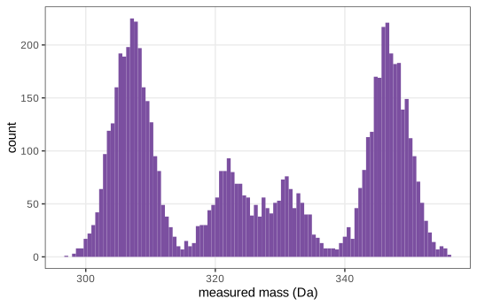
fig_4_10. Reproduces Holmes and Huber (2019), Figure 4.10. Download: PDF · SVGFilling the gap 4.9: when do the components show? Section 4.2.4, Questions 4.9 to 4.11
The theoretical density asked for in Question 4.11 is
\[ f(x)=0.12\,\phi(x\given331,\sigma^2)+0.38\,\phi(x\given307,\sigma^2)+0.36\,\phi(x\given347,\sigma^2)+0.14\,\phi(x\given322,\sigma^2). \]Sorted, the masses are 307, 322, 331, 347, with gaps of 15, 9 and 16 Da. Result 4.1(b) says that two equal-weight equal-variance neighbours stay separate modes only if their gap exceeds \(2\sigma\). With \(\sigma=3\) every gap exceeds \(2\sigma=6\), and the density has 4 modes; with \(\sigma=10\) (Question 4.10) every gap is below \(2\sigma=20\) and the density computed on a fine grid has only 2 modes. The criterion is a guide rather than a theorem for unequal weights, but it explains the pictures. With \(N=1000\) instead of 7000 (Question 4.9) the density is the same but each of the 100 histogram bins holds about 10 values, so the bin counts fluctuate by about \(\sqrt{10}\approx3\) and the smaller components (A and T) are hard to tell from noise.
4.3 Empirical distributions and the nonparametric bootstrap
The most extreme mixture puts one component on each observation. Darwin's Zea mays experiment compared the heights of 15 pairs of plants, one cross-fertilised and one self-fertilised in each pair; the 15 differences (in inches) are the data.
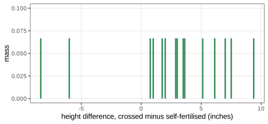
fig_4_11. Reproduces Holmes and Huber (2019), Figure 4.11. Download: PDF · SVGDefinition 4.3 (empirical distribution) Section 4.3, (4.11), (4.12)
The empirical distribution \(\hat F_n\) of \(x_1,\dots,x_n\) is the mixture of \(n\) point masses of weight \(1/n\) at the observations. Its cumulative distribution function, the ECDF, is
\[ \hat F_n(t)=\frac1n\sum_{i=1}^n\ind\{x_i\le t\}, \tag{4.11} \]and its "density" is the corresponding combination of point masses,
\[ \hat f_n=\frac1n\sum_{i=1}^n\delta_{x_i},\qquad\text{meaning}\quad\int g\,\d\hat F_n=\frac1n\sum_{i=1}^ng(x_i)\ \text{for every function } g. \tag{4.12} \]The book prints the indicator in (4.11) as \(\ind_{x\le x_i}\), which would count the observations at or above \(x\) and give a decreasing function; the ECDF counts the observations at or below its argument.
Filling the gap 4.10: statistics as functions of \(\hat F_n\) Section 4.3
The book's "derivative of a step function" is made precise by the Lebesgue-Stieltjes integral: for a distribution function \(F\), \(\int g\,\d F=\E_F\,g(X)\). For \(\hat F_n\), a step function with jumps of \(1/n\) at the data, this integral is the average in (4.12). Many statistics are functionals \(T\) of a distribution evaluated at \(\hat F_n\) (plug-in estimates):
- the mean, \(T(F)=\int t\,\d F(t)\): \(T(\hat F_n)=\bar x\) (the book's formula \(\bar x=\int\delta_{x_i}(x)\,\d x\) is a misprint: that integral equals 1);
- the variance, \(T(F)=\int(t-\int s\,\d F)^2\d F(t)\): \(T(\hat F_n)=\frac1n\sum(x_i\)
\({}-\bar x)^2\), the divide-by-\(n\) variance; - the median, \(T(F)=F^{-1}(1/2)\)
\({}=\inf\{t:F(t)\) \({}\ge\tfrac12\}\): for odd \(n\), \(T(\hat F_n)=x_{((n+1)/2)}\), the middle order statistic.
This is the plug-in principle: estimate a feature of \(F\) by the same feature of \(\hat F_n\). It works because \(\hat F_n\) is close to \(F\) (Result 4.5).
Result 4.5 (\(\hat F_n\) converges to \(F\) uniformly) Section 4.3
For independent observations from any distribution function \(F\): (a) for each \(t\), \(n\hat F_n(t)\sim\Bin(n,F(t))\), so \(\hat F_n(t)\) is unbiased with variance \(F(t)\{1-F(t)\}/n\); (b) Glivenko-Cantelli: \(\sup_t|\hat F_n(t)-F(t)|\to0\) almost surely; (c) Dvoretzky-Kiefer-Wolfowitz with Massart's constant: for every \(\varepsilon>0\),
\[ \Pr\Big(\sup_t|\hat F_n(t)-F(t)|>\varepsilon\Big)\le2e^{-2n\varepsilon^2}. \]Proof of (a) and (b); (c) is quoted
(a) The indicators \(\ind\{x_i\le t\}\) are independent Bernoulli(\(F(t)\)). (b) By the strong law, \(\hat F_n(t)\to F(t)\) and \(\hat F_n(t^-)\to F(t^-)\) almost surely for each fixed \(t\). Given \(\varepsilon\), choose finitely many points \(-\infty=t_0<t_1\)
For the 15 Zea mays differences, (c) with \(\varepsilon=0.35\) gives a 95% confidence band \(\hat F_n\pm0.35\) for the whole distribution function: a reminder that 15 observations pin down \(F\) only coarsely, which limits any bootstrap built on them.
A statistic \(\hat\tau\) computed from data varies from sample to sample; its sampling distribution (book Figure 4.12) describes that variation, but we observe only one sample. The bootstrap replaces the unknown \(F\) by \(\hat F_n\) (book Figure 4.13).
Definition 4.4 (nonparametric bootstrap) Section 4.3
Let \(\hat\tau=T(x_1,\dots,x_n)\). A bootstrap sample \(x_1^*,\dots,x_n^*\) is a sample of size \(n\) from \(\hat F_n\), i.e. drawn with replacement from the data. The bootstrap distribution of \(\hat\tau\) is the distribution of \(\hat\tau^*=T(x_1^*,\dots,x_n^*)\) given the data. The bootstrap standard error is its standard deviation, and the percentile interval at level \(1-\alpha\) is \([\hat G^{-1}(\alpha/2),\hat G^{-1}(1\)
Algorithm 4.3 (Monte Carlo bootstrap) Section 4.3, Figure 4.14
- For \(b=1,\dots,B\): draw indices \(i_1,\dots,i_n\) independently and uniformly from \(\{1,\dots,n\}\) and compute \(\hat\tau^*_b\)
\({}=T(x_{i_1},\dots,x_{i_n})\). - Bootstrap standard error: the standard deviation of \(\hat\tau^*_1,\dots,\hat\tau^*_B\).
- Percentile interval: the empirical \(\alpha/2\) and \(1-\alpha/2\) quantiles of the \(\hat\tau^*_b\).
Filling the gap 4.11: plug-in, two kinds of error, and how many resamples there are Section 4.3, Questions 4.14 and 4.15
The bootstrap is a plug-in estimate. The standard error of \(\hat\tau\) is a functional of \(F\): \(\operatorname{se}_F(\hat\tau)\)
Two errors (Question 4.15). The Monte Carlo estimate differs from what we want for two reasons:
\[ \hat{\operatorname{se}}_B-\operatorname{se}_F=\underbrace{(\hat{\operatorname{se}}_B-\operatorname{se}_{\hat F_n})}_{\text{Monte Carlo error}}+\underbrace{(\operatorname{se}_{\hat F_n}-\operatorname{se}_F)}_{\text{bootstrap (statistical) error}} . \]The first is controlled by \(B\): for approximately normal \(\hat\tau^*\) the standard deviation of \(\hat{\operatorname{se}}_B\) is about \(\operatorname{se}_{\hat F_n}/\sqrt{2(B-1)}\), about 2% for \(B=1000\), and tail quantiles need larger \(B\) (several thousand for a 99% interval). The second is fixed by the data: it shrinks only with \(n\), and no \(B\) removes it. In the bootstrap package, nboot controls the first.
How many different resamples (Question 4.14). A resample is determined, for a symmetric statistic, by the multiplicities \(k_1,\dots,k_n\ge0\) with \(\sum k_i=n\). Represent it as a row of \(n\) balls and \(n-1\) bars (the balls before the first bar go to observation 1, and so on): a bijection with the choices of \(n-1\) bar positions among \(2n-1\) places, so there are
\[ \binom{2n-1}{n-1}\ \text{resamples:}\quad 10\ (n=3),\qquad 77{,}558{,}760\ (n=15). \](Brute-force enumeration for \(n=3,4,5\) gives 10, 35, 126.) They are not equally likely: a resample with multiplicities \(k\) has the multinomial probability \(n!/(k_1!\cdots k_n!)\,n^{-n}\), from \(n!\,n^{-n}\approx3.0\times10^{-6}\) for the original sample itself (\(n=15\)) down to \(n^{-n}\) for "all copies of one point". The exhaustive bootstrap must weight them accordingly.
Result 4.6 (exact bootstrap distributions of the mean and the median) Section 4.3, Figure 4.14, Questions 4.12 and 4.13
(a) Mean. Given the data, \(\E^*\bar x^*=\bar x\) and \(\var^*\bar x^*=\hat\sigma^2/n\) with \(\hat\sigma^2\)
(b) Median. Let \(n=2m-1\) be odd and the data distinct, with order statistics \(x_{(1)}<\dots<x_{(n)}\). The bootstrap median takes only the values \(x_{(j)}\), and
\[ \Pr{}^*\big(\median(x^*)\le x_{(j)}\big)=\Pr\Big(\Bin\big(n,\tfrac jn\big)\ge m\Big)=\sum_{k=m}^n\binom nk\Big(\frac jn\Big)^k\Big(1-\frac jn\Big)^{n-k}. \]Proof
(a) \(\bar x^*=\frac1n\sum x_i^*\) with the \(x_i^*\) independent, each uniform on the data, so each has mean \(\bar x\) and variance \(\hat\sigma^2\).
(b) The median of the resample is its \(m\)-th smallest value, which is one of the data values. It is at most \(x_{(j)}\) exactly when at least \(m\) of the \(n\) draws are at most \(x_{(j)}\). Each draw is at most \(x_{(j)}\) with probability \(j/n\), independently, so the number of such draws is \(\Bin(n,j/n)\). ∎
Zea mays. The data have mean 2.617 and median 3. The exact bootstrap standard error of the mean is \(\hat\sigma/\sqrt{15}=1.177\) (the \(t\)-test standard error with divisor 14 is 1.218); that of the median is 0.998, with the median's bootstrap distribution concentrated on 2.875, 3, 3.5 (probabilities 0.183, 0.207, 0.183). The exact 99% percentile interval for the median is \([1, 6.125]\), the same as the 95% interval because the distribution is discrete, and it excludes 0 (Question 4.12): crossed plants grow taller. 200,000 resamples reproduce the exact probabilities to within 0.0011; the 1,000 resamples of Figure 4.14 give a standard error of 1.017.
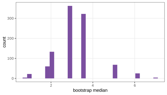
fig_4_14. Reproduces Holmes and Huber (2019), Figure 4.14. Download: PDF · SVGQuestions 4.12 and 4.13 (interval for the median; mean versus median)
Find a 99% bootstrap interval for the median; then compare the bootstrap distributions of the mean and the median.
Answer
From the 1,000 resampled medians of Figure 4.14, the 0.5% and 99.5% quantiles are 1 and 6.125, as in the exact computation of Result 4.6; the interval lies above 0, so the data support a positive median difference. The bootstrap distribution of the mean is smooth and close to normal (standard error 1.18; a sum of 15 independent draws), while that of the median is discrete and lumpy, supported on the data values and concentrated on the middle five. For these data the median is slightly less variable (standard error 1.00 against 1.18) because two large negative differences (\(-8.4\) and \(-6\)) inflate the variance of the mean but barely move the median.
Result 4.7 (why the bootstrap works: the mean) Section 4.3
Let \(X_1,X_2,\dots\) be independent with distribution \(F\), mean \(\mu\) and finite variance \(\sigma^2>0\). Then, for almost every data sequence,
\[ \sup_t\Big|\Pr{}^*\big(\sqrt n(\bar x^*-\bar x)\le t\big)-\Pr\big(\sqrt n(\bar X-\mu)\le t\big)\Big|\to0 , \]where \(\Pr^*\) is the bootstrap probability given \(x_1,\dots,x_n\) (Bickel and Freedman 1981; Singh 1981). The bootstrap distribution of the centred mean is a consistent estimate of its sampling distribution.
Proof
Both distributions converge to \(\N(0,\sigma^2)\), and convergence to a continuous limit is uniform in \(t\) (Pólya's theorem); so it suffices to show the bootstrap statement. Given the data, \(\sqrt n(\bar x^*\)
For any fixed \(M\) and \(n\) large enough that \(\varepsilon\sqrt n>M\), the right side is at most \(\frac1n\sum_j(x_j\)
Beyond the mean. The same conclusion holds for smooth functions of means (by the delta method, Filling the gap 4.16) and for sample quantiles such as the median of a distribution with a positive continuous density at the median. It fails for statistics that depend on the extremes, such as the sample maximum, and for heavy-tailed data without a finite variance. In practice the bootstrap is a first-order approximation; its accuracy for small \(n\), as with 15 plants, is limited by how well \(\hat F_n\) represents \(F\).
Why "nonparametric"? The bootstrap model \(\hat F_n\) has \(n\) free point masses, as many parameters as observations; in that sense it is a nonparametric method, although it estimates plenty of parameters. The parametric bootstrap would instead resample from a fitted model \(F_{\hat\theta}\).
4.4 Infinite mixtures
Mixtures are useful even when nobody wants to label the observations: letting a parameter of a simple distribution vary continuously from observation to observation produces new, more flexible distributions.
Definition 4.5 (continuous or infinite mixture) Section 4.4
Let \(\{f(\cdot\given\vartheta)\}\) be a family of densities and \(G\) a distribution of the parameter \(\vartheta\) (the mixing distribution). The mixture
\[ f_G(x)=\int f(x\given\vartheta)\,\d G(\vartheta) \]is the distribution of \(X\) in the two-level scheme \(\vartheta\sim G\), \(X\given\vartheta\sim f(\cdot\given\vartheta)\). A finite mixture is the case of a discrete \(G\) with finitely many atoms; "infinite" refers to a \(G\) with infinitely many (typically a continuum of) values. The book's informal criterion, "as many components as observations", describes how such models behave on data: every observation has its own parameter value.
4.4.1 Infinite mixture of normals
Draw \(W\) from an exponential distribution and use it as the variance of a normal: \(W\sim\Exp(1)\), \(X\given W\sim\N(\mu,W)\). The result is the Laplace distribution (book Figure 4.15, a portrait of Laplace, is not reproduced), whose density with location \(\theta\) and scale \(\phi>0\) is
\[ f(y)=\frac1{2\phi}\exp\Big(-\frac{|y-\theta|}{\phi}\Big). \]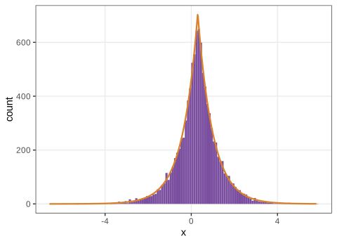
fig_4_16. Reproduces Holmes and Huber (2019), Figure 4.16. Download: PDF · SVGResult 4.8 (the Laplace distribution is a normal variance mixture) Section 4.4.1, Question 4.16, (4.13)
If \(W\sim\Exp(\lambda)\) (rate \(\lambda\), mean \(1/\lambda\)) and \(X\given W\sim\N(\theta,W)\), then \(X\sim\Lap(\theta,\phi)\) with \(\phi=1/\sqrt{2\lambda}\). In particular (Question 4.16)
\[ X=\sqrt W\,Z,\qquad W\sim\Exp(1),\ Z\sim\N(0,1)\ \text{independent}, \tag{4.13} \]is Laplace with \(\theta=0\) and \(\phi=1/\sqrt2\), so its variance \(2\phi^2=1=\E W\).
Proof
By the characteristic function. Conditioning on \(W\), \(\E e^{it(X-\theta)}\)
By direct integration. With \(d=x-\theta\), \(f(x)=\int_0^\infty(2\pi w)^{-1/2}e^{-d^2/(2w)}\lambda e^{-\lambda w}\d w\). The identity of Filling the gap 4.12 with \(a=d^2/2\), \(b=\lambda\) gives \(f(x)=\lambda(2\pi)^{-1/2}\sqrt{\pi/\lambda}\,e^{-2\sqrt{\lambda d^2/2}}\)
A Kolmogorov-Smirnov test of 200,000 simulated values of (4.13) against \(\Lap(0,1/\sqrt2)\) does not reject, and the orange curve in Figure 4.16 is this density. Andrews and Mallows (1974) characterised all such normal scale mixtures; the Student \(t\) distribution is another one (inverse-gamma mixing).
Filling the gap 4.12: an integral that keeps appearing Section 4.4.1
For \(a\ge0\) and \(b>0\),
\[ \int_0^\infty w^{-1/2}\exp\Big(-\frac aw-bw\Big)\d w=\sqrt{\frac\pi b}\,e^{-2\sqrt{ab}} . \]Proof. Substitute \(w=u^2\) (\(w^{-1/2}\d w=2\,\d u\)) and complete the square, \(a/u^2+bu^2=(\sqrt b\,u\)
Call the last integral \(J\). The substitution \(u=\sqrt{a/b}/v\) maps \((0,\infty)\) to itself, leaves \((\sqrt bu-\sqrt a/u)^2\) unchanged and gives \(J=\int_0^\infty e^{-(\sqrt bv-\sqrt a/v)^2}\sqrt{a/b}\,v^{-2}\d v\). Averaging the two expressions, \(J=\frac1{2\sqrt b}\int_0^\infty e^{-y(u)^2}(\sqrt b\)
Filling the gap 4.13: estimating the Laplace parameters, and the lasso Section 4.4.1, Figure 4.15
The log-likelihood of \(\Lap(\theta,\phi)\) is \(\ell(\theta,\phi)\)
Location. For any \(\phi\), maximising over \(\theta\) means minimising \(S(\theta)=\sum_i|x_i-\theta|\), a convex piecewise linear function with slope \(\#\{x_i<\theta\}\)
Scale. \(\partial\ell/\partial\phi\)
Correction. The book's caption of Figure 4.15 says the scale parameter is the median absolute deviation (MAD). Under the Laplace model \(|X-\theta|\sim\Exp\) with mean \(\phi\), whose median is \(\phi\log2\); so the MAD estimates \(0.693\,\phi\), and the maximum-likelihood estimate of \(\phi\) is the mean absolute deviation. On the 10,000 values of Figure 4.16 (true \(\theta=0.3\), \(\phi=0.707\)): median 0.306, mean absolute deviation 0.710, median absolute deviation 0.489 (\(=0.707\log2=0.490\)).
Lasso and ridge. In a regression \(y=\mathbf X\beta+\varepsilon\), \(\varepsilon\sim\N(0,\sigma^2\mathbf I)\), with independent \(\Lap(0,\phi)\) priors on the coefficients, the negative log posterior is \(\|y-\mathbf X\beta\|^2/(2\sigma^2)\)
Asymmetric Laplace. Letting the mean drift with the variance gives the asymmetric Laplace distribution: \(W\sim\Exp(1)\) and \(X\given W\sim\N(\theta\)
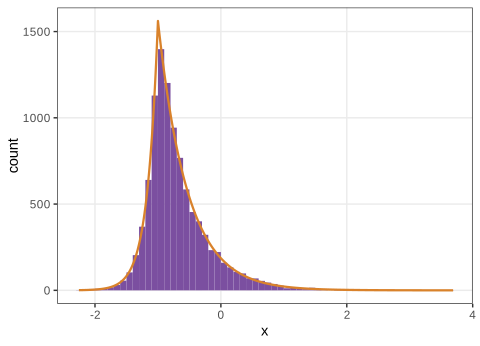
fig_4_17. Reproduces Holmes and Huber (2019), Figure 4.17. Download: PDF · SVGResult 4.9 (the asymmetric Laplace distribution) Section 4.4.1, (4.14), Figure 4.17
For \(X\sim\AL(\theta,\mu,\sigma)\) with \(s=\sqrt{2\sigma^2+\mu^2}\) and \(d=x-\theta\),
\[ f(x)=\frac1s\exp\Big\{\frac{\mu d-s|d|}{\sigma^2}\Big\}, \qquad \E X=\theta+\mu,\qquad \var X=\sigma^2+\mu^2 . \tag{4.14} \]The density is two exponential tails glued at the mode \(\theta\), with rates \((s-\mu)/\sigma^2\) to the right and \((s+\mu)/\sigma^2\) to the left; for \(\mu=0\), \(\sigma=1\) it is Result 4.8.
Proof
Moments. \(\E X=\E\{\E(X\given W)\}\)
Density. \(f(x)=\int_0^\infty(2\pi\sigma^2w)^{-1/2}\exp\{-(d\)
using \(1+\mu^2/(2\sigma^2)\)
The variance is \(\sigma^2+(\E X-\theta)^2\): it depends on the mean, unless \(\mu=0\). The book uses such hierarchical models for the lengths of yeast promoters and for microarray log-ratios (its Figure 4.18, two histograms shown as images; the underlying data are not distributed with the book, so the figure is not reproduced). The density agrees with numerical integration of the mixture (to \(3\times10^{-13}\)) and the moments with simulation.
Question 4.17 (why are microarray log-ratios Laplace-like?)
Answer
A log-ratio of two intensities is roughly normal for a given gene, but the noise level differs from gene to gene (bright spots are measured more precisely than faint ones, probes differ in quality). A histogram over 20,000 genes is therefore a mixture of normals with different variances, which by Result 4.8 has a sharper peak and heavier, exponential tails than any single normal; a gene-dependent shift that grows with the variance (for example from intensity-dependent dye bias) makes it skewed, the asymmetric Laplace.
4.4.2 Infinite mixtures of Poisson variables
Counts in ecology and sequencing follow the same two-level pattern: given its true abundance, the count in one sample is Poisson (or binomial), but the abundance itself varies between lakes, between biological replicates or along the genome. The Poisson rate becomes a random variable with its own distribution, and further levels (species, environmental covariates) can be stacked on top. The convenient choice for the rate distribution is the gamma family (book Figure 4.19, an artwork, is not reproduced).
4.4.3 Gamma distribution: two parameters (shape and scale)
Definition 4.6 (gamma distribution) Section 4.4.3, (4.16)
\(X\sim\Gam(a,b)\), shape \(a>0\) and rate \(b>0\) (scale \(1/b\)), has density
\[ f_\Gamma(x;a,b)=\frac{b^a}{\Gamma(a)}x^{a-1}e^{-bx},\quad x>0,\qquad \Gamma(a)=\int_0^\infty x^{a-1}e^{-x}\,\d x. \tag{4.16} \]\(\Gam(1,b)=\Exp(b)\), and a sum of \(a\) independent \(\Exp(b)\) variables is \(\Gam(a,b)\) for integer \(a\).
Filling the gap 4.14: moments and shape of the gamma Section 4.4.3, Figure 4.20
Using \(\int_0^\infty x^{c-1}e^{-bx}\d x\)
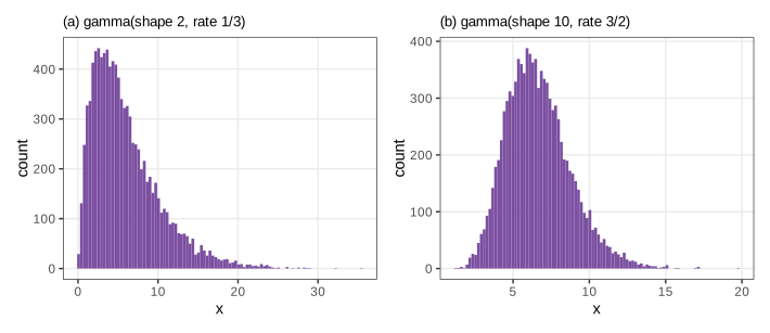
fig_4_20. Reproduces Holmes and Huber (2019), Figure 4.20. Download: PDF · SVGThe gamma-Poisson hierarchical model. Draw rates \(\lambda_1,\lambda_2,\dots\) from a gamma distribution and, for each, a count from \(\Pois(\lambda_i)\). The counts (Figure 4.21) are integers: the mixture of discrete distributions is discrete (Question 4.18).
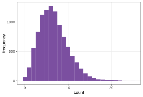
fig_4_21. Reproduces Holmes and Huber (2019), Figure 4.21. Download: PDF · SVGDefinition 4.7 (negative binomial, or gamma-Poisson, distribution) Section 4.4.3, (4.15)
For \(a>0\) and \(p\in(0,1]\), \(K\sim\NB\) has probability mass function
\[ \Pr(K=k)=\binom{k+a-1}{k}p^a(1-p)^k=\frac{\Gamma(k+a)}{\Gamma(a)\,k!}\,p^a(1-p)^k,\qquad k=0,1,2,\dots \tag{4.15} \](the binomial coefficient for non-integer \(a\) is defined through the gamma function). Its mean is \(\mu=a(1-p)/p\); in the mean parametrisation, \(p=a/(a+\mu)\), the size \(a\) and the dispersion \(\alpha=1/a\). In R, dnbinom(k, size = a, prob = p) or dnbinom(k, size = a, mu = mu). For integer \(a\), \(K\) counts the failures before the \(a\)-th success in independent trials with success probability \(p\); the name comes from the negative binomial series \(\sum_k\binom{k+a-1}{k}q^k\)
Result 4.10 (gamma mixture of Poissons) Section 4.4.3, Question 4.19
If \(\lambda\sim\Gam(a,b)\) and \(K\given\lambda\sim\Pois(\lambda)\), then \(K\) has the negative binomial distribution (4.15) with size \(a\) and \(p=b/(b+1)\). Its mean and variance are
\[ \E K=\mu=\frac ab=\frac{a(1-p)}{p},\qquad \var K=\mu+\frac{\mu^2}{a}=\mu+\alpha\mu^2 . \]The variance exceeds the Poisson variance \(\mu\) by \(\var\lambda=\alpha\mu^2\), the variance of the mixing distribution. As \(a\to\infty\) with \(\mu\) fixed, \(\NB(\mu,a)\to\Pois(\mu)\).
Proof
Distribution. Integrate the Poisson probability against the gamma density:
\[ \Pr(K=k)=\int_0^\infty\frac{x^ke^{-x}}{k!}\,\frac{b^a}{\Gamma(a)}x^{a-1}e^{-bx}\,\d x=\frac{b^a}{\Gamma(a)\,k!}\int_0^\infty x^{k+a-1}e^{-(b+1)x}\d x=\frac{b^a}{\Gamma(a)\,k!}\,\frac{\Gamma(k+a)}{(b+1)^{k+a}}, \]which is \(\frac{\Gamma(k+a)}{\Gamma(a)k!}\big(\frac b{b+1}\big)^a\big(\frac1{b+1}\big)^k\), i.e. (4.15) with \(p=b/(b+1)\), \(1-p=1/(b+1)\). (Interchanging nothing is needed: the integrand is non-negative.)
Moments. \(\E K=\E\{\E(K\given\lambda)\}\)
Poisson limit. With \(p=a/(a+\mu)\), \(\Pr(K=k)=\frac{\Gamma(k+a)}{\Gamma(a)a^k}\,\frac{\mu^k}{k!}\,\big(1\)
The integral agrees with dnbinom to \(10^{-16}\) for \(a=10\), \(b=3/2\) and \(k\le30\).
Correction: the mean of the negative binomial Section 4.4.3, text after (4.15)
The book gives the mean as \(\mu=pa/(1-p)\). For (4.15) the mean is \(a(1-p)/p\) (Result 4.10): with \(a=10\), \(p=0.6\) the printed formula gives 15, the correct mean is 6.67 (and the sample mean of Figure 4.21 is 6.65). The printed formula is the mean when \(p\) is the probability of a "failure" rather than of a "success", the opposite of (4.15) and of R's prob. The variance \(\mu+\alpha\mu^2\) quoted by the book is correct.
Questions 4.18 and 4.19 (discrete or continuous; another name; the derivation)
Answer
The values are discrete: each is a Poisson count. The distribution is the negative binomial, and vcd::goodfit(gp, "nbinomial") estimates size 10.15 and prob 0.604 from the 10,000 simulated values, close to the generating \(a=10\), \(p=b/(b+1)=0.6\) (Figure 4.22). The analytical derivation is the proof of Result 4.10.
Filling the gap 4.15: fitting the negative binomial Section 4.4.3, Figure 4.22
In the mean parametrisation the log-likelihood of counts \(x_1,\dots,x_n\) is
\[ \ell(\mu,a)=\sum_i\Big\{\log\Gamma(x_i+a)-\log\Gamma(a)-\log x_i!+a\log\frac{a}{a+\mu}+x_i\log\frac{\mu}{a+\mu}\Big\}. \]The mean. \(\partial\ell/\partial\mu\)
The size. The profile \(\ell(\bar x,a)\) is then maximised over the single parameter \(a\) (or \(\log a\)) numerically; the course code uses a one-dimensional search. A quick alternative is the method of moments, which matches \(s^2=\bar x+\bar x^2/a\): \(\tilde a=\bar x^2/(s^2-\bar x)\), defined only when the sample is overdispersed (\(s^2>\bar x\)); otherwise the Poisson (\(a=\infty\)) is the best fit. For the 10,000 values of Figure 4.21, \(\bar x=6.652\), \(s^2=11.057\), so \(\tilde a=10.05\), against the maximum-likelihood size 10.15 reported by goodfit and the true 10. For the ChIP-Seq bins of Section 4.2.3 the maximum-likelihood size is 0.696: overdispersion far beyond any Poisson.
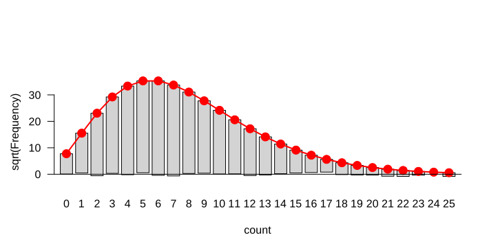
vcd::goodfit (size 10.15, prob 0.604): bars of height \(\sqrt{\text{observed}}\) hang from the fitted \(\sqrt{\text{expected}}\) (red); their bottoms stay close to zero, a good fit. Code: ch04_mixture_models.R, fig_4_22. Reproduces Holmes and Huber (2019), Figure 4.22. Download: PDF · SVGFigure 4.23 shows the two levels at once: the gamma distribution of the latent rate, one Poisson distribution given one realised rate, and the resulting gamma-Poisson distribution of the counts.
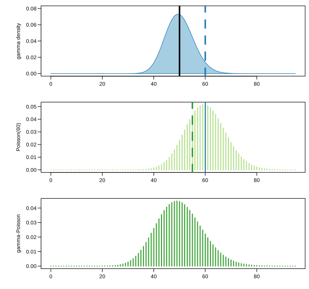
fig_4_23. Reproduces Holmes and Huber (2019), Figure 4.23. Download: PDF · SVG4.4.4 Variance stabilizing transformations
Replicate measurements of the same quantity vary, and the amount of variation decides whether a difference between conditions is visible. In hierarchical count models the variance depends on the mean (heteroscedasticity): Poisson counts with mean 10 have standard deviation 3.2, with mean 100 standard deviation 10. Methods that assume a common variance (regression, \(t\)-tests, PCA, clustering) then give too much weight to the high counts.
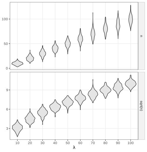
fig_4_24. Reproduces Holmes and Huber (2019), Figure 4.24. Download: PDF · SVGDefinition 4.8 (variance-stabilising transformation) Section 4.4.4
Let \(X\) have mean \(\mu\) and variance \(v(\mu)\), a known function of the mean. A smooth increasing function \(g\) is variance stabilising if \(\var g(X)\) is (approximately) the same for all \(\mu\) in the range of interest. If \(g\) is one, so is \(cg+d\) for constants \(c\ne0\), \(d\).
Result 4.11 (the delta method and the stabilising transformation) Section 4.4.4, (4.17)–(4.19)
If the standard deviation of \(X\) is small compared with the scale over which \(g'\) changes near \(\mu\), then
\[ g(X)\approx g(\mu)+g'(\mu)(X-\mu), \tag{4.17} \] \[ \var g(X)\approx g'(\mu)^2\var X=g'(\mu)^2\,v(\mu). \tag{4.18} \]The variance is constant, equal to \(c^2\), when
\[ g'(x)=\frac{c}{\sqrt{v(x)}},\qquad g(x)=\int^x\frac{c\,\d t}{\sqrt{v(t)}} . \tag{4.19} \]- Poisson, \(v(\mu)=\mu\): \(g(x)=2c\sqrt x\); with \(c=\tfrac12\), \(\sqrt X\) has variance close to \(\tfrac14\) (Figure 4.24); \(2\sqrt X\) has variance close to 1.
- Constant coefficient of variation, \(v(\mu)=\alpha\mu^2\): \(g(x)=(c/\sqrt\alpha)\log x\). This is why logarithms are the default for intensities whose standard deviation is proportional to the mean.
- Gamma-Poisson, \(v(\mu)=\mu+\alpha\mu^2\): \(g_\alpha(x)=\asinh(\sqrt{\alpha x})/\sqrt\alpha\) with \(c=\tfrac12\) (Filling the gap 4.18), which behaves like \(\sqrt x\) for \(\alpha x\ll1\) and like \(\frac1{2\sqrt\alpha}\log(4\alpha x)\) for \(\alpha x\gg1\).
Filling the gap 4.16: what the delta method guarantees, and where it is off Section 4.4.4, (4.17), (4.18)
The asymptotic statement. The book's "neglect higher-order terms" is made precise by the delta method: if \((X_\lambda-\mu_\lambda)/\sqrt{v(\mu_\lambda)}\Rightarrow\N(0,1)\) as some index \(\lambda\to\infty\), and \(g\) is differentiable with \(g'\) varying slowly on the scale \(\sqrt{v}\), then \(\{g(X_\lambda)\)
since \(X/\lambda\to1\) in probability (Slutsky's lemma). Convergence in distribution does not by itself give convergence of variances, but here the moments converge too, and a second-order expansion gives \(\var\sqrt X=\tfrac14\)
When the mixing noise dominates. For gamma-Poisson counts with fixed size \(a\) and \(\mu\to\infty\), the Poisson noise becomes negligible relative to the gamma noise: \(X/\mu\Rightarrow G\sim\Gam(a,a)\) (mean 1). Then \(g_\alpha(X)=\frac{1}{2\sqrt\alpha}\log X\)
where \(\psi'\) is the trigamma function (the variance of \(\log G\) for a gamma variable). The delta method instead linearises \(\log G\) around 1, giving \(\var(\log G)\approx\var G=1/a\) and hence \(\tfrac14\). Since \(\psi'(a)=1/a+1/(2a^2)+O(a^{-3})\), the two agree for large \(a\), but for \(a=4\) the exact limit is \(\sd=\sqrt{4\psi'(4)}/2=0.5328\), not 0.5: the noise of the gamma level is too large for a first-order expansion. Numerically, the standard deviation is 0.5328 at \(\mu=2^{14}\), to \(10^{-4}\).
Gamma-Poisson counts with size 4 and means from 1 to 1024 (Figure 4.25) show the problem in a stronger form: the standard deviation grows like the mean once \(\mu>a\), because \(v(\mu)=\mu+\mu^2/4\).
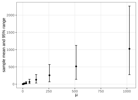
fig_4_25. Reproduces Holmes and Huber (2019), Figure 4.25. Download: PDF · SVGQuestion 4.20 (a transformation for Figure 4.25, built from the data)
Find a transformation that stabilises the variance of the counts of Figure 4.25.
Answer
Divide the counts near each mean by their standard deviation, and join these local rescalings into one continuous increasing piecewise linear function with slope \(1/\sd(\mu_i)\) around \(\mu_i\). That is a Riemann sum for (4.19): see Filling the gap 4.17 and Figure 4.26. Its shape resembles a square root at small means and a logarithm at large means, which is what Result 4.11 predicts for \(v(\mu)=\mu+\mu^2/4\).
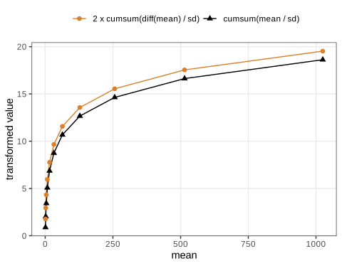
cumsum(mean / sd) (black) and twice the Riemann sum of \(1/\mathrm{sd}\) (orange). They are nearly proportional because the means double (Filling the gap 4.17). Code: ch04_mixture_models.R, fig_4_26. Reproduces Holmes and Huber (2019), Figure 4.26. Download: PDF · SVGFilling the gap 4.17: the piecewise linear construction, and why the book's version works Section 4.4.4, Figure 4.26
Integrating \(g'(\mu)=1/\sd(\mu)\) with the left-endpoint rule on the grid \(\mu_0=0<\mu_1<\dots<\mu_m\) of observed means gives
\[ g(\mu_j)\approx\sum_{i=1}^j\frac{\mu_i-\mu_{i-1}}{\sd(\mu_i)}, \]a continuous piecewise linear function with slope \(1/\sd(\mu_i)\) on \([\mu_{i-1},\mu_i]\). The book's code computes cumsum(mean / sd), that is \(\sum_{i\le j}\mu_i/\sd(\mu_i)\): it multiplies each slope by \(\mu_i/(\mu_i-\mu_{i-1})\) instead of the interval length. For the book's grid \(\mu_i=2^{i}\) that factor is exactly 2 for every \(i\ge1\) (\(\mu_i-\mu_{i-1}=\mu_i/2\)), so the book's function is twice the Riemann sum up to the first term, and a constant multiple of a stabilising transformation is still one (Definition 4.8). On a non-geometric grid the same code would not stabilise the variance. Figure 4.26 draws both versions; numerically the factor is 2 (increment ratios between 1.96 and 2.02 with the simulated means).
Filling the gap 4.18: the stabilising transformation for gamma-Poisson counts Section 4.4.4, Question 4.21, (4.20)–(4.22)
We need
\[ \int\frac{\d x}{\sqrt{x+\alpha x^2}}. \tag{4.20} \]The book quotes a table integral for \(\int\d x/\sqrt{ax^2+bx+c}\),
\[ \int\frac{\d x}{\sqrt{ax^2+bx+c}}=\frac1{\sqrt a}\log\Big(2\sqrt{a(ax^2+bx+c)}+2ax+b\Big)+\const\quad(a>0). \tag{4.21} \]A self-contained route: substitute \(x=\sinh^2(u)/\alpha\), \(u\ge0\). Then \(\d x=2\sinh u\cosh u\,\d u/\alpha\) and \(x+\alpha x^2\)
The three forms agree. \(\cosh2u=1+2\sinh^2u\) gives \(\acosh(1+2\alpha x)\)
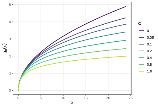
fig_4_27. Reproduces Holmes and Huber (2019), Figure 4.27. Download: PDF · SVGSummary
- Finite mixtures are the distributions of two-step experiments: a hidden label, then an observation. Their moments come from the laws of total expectation and variance, and they are identifiable only up to relabelling. A two-component equal-variance mixture shows two modes only when the means are more than two standard deviations apart.
- EM maximises a likelihood with hidden variables by alternating posterior membership weights and weighted maximum likelihood. It never decreases the likelihood (Jensen's inequality), converges linearly at a rate set by the fraction of missing information, and can stop at saddle points or local maxima, so it should be started several times. The normal-mixture likelihood is unbounded, and "the" estimate is a well-behaved local maximum.
- Zero inflation is a mixture with a point mass at zero; EM gives each zero a posterior probability of being structural. On ChIP-Seq bins neither the Poisson nor the zero-inflated Poisson fits; the gamma-Poisson captures the long tail.
- The empirical distribution is a mixture of \(n\) point masses and converges uniformly to the truth. The bootstrap is the plug-in estimate of a sampling distribution; it has a Monte Carlo error controlled by \(B\) and a statistical error controlled only by \(n\). For the mean and the median its answer is available exactly.
- Infinite mixtures build distributions: exponential mixtures of normal variances give the (asymmetric) Laplace, gamma mixtures of Poisson rates give the negative binomial with variance \(\mu+\alpha\mu^2\). The resulting mean-variance relations call for variance-stabilising transformations \(g'\propto1/\sqrt{v}\): the square root, the logarithm and \(\asinh(\sqrt{\alpha x})/\sqrt\alpha\). The delta method behind them is first order; for strongly overdispersed counts the stabilised standard deviation is \(\sqrt{a\psi'(a)}/2\) rather than \(1/2\).
Exercises
Exercise 4.1 (the EM algorithm step by step). The file
Myst.rdsholds 1,800 values (Figure 4.28). Model them as a mixture of two normal components A and B with unknown means, standard deviations and mixing fraction. Starting from random membership weights, run the book's loop: (a) which lines are the E step and which the M step? (b) What dotolerance,miniterandmaxiterdo? (c) Compare withmixtools::normalmixEM.Solution
(a) The loop starts with the M step (the book starts from weights, not parameters): \(\lambda\) is the mean of the weights of A, the means are weighted means, the standard deviations weighted root-mean-square deviations, exactly the formulas of Filling the gap 4.6 with \(r_{iA}\) =
wA. The E step follows:pAandpBare \(\lambda\phi_A(x_i)\) and \((1-\lambda)\phi_B(x_i)\), andwA = pA / (pA + pB)is (4.5). The log-likelihoodsum(log(pA + pB))is that of the parameters just estimated, (4.6).(b) The loop stops when the log-likelihood changes by at most
tolerance(\(10^{-12}\)), but runs at leastminiteriterations (so that a slow start is not mistaken for convergence) and at mostmaxiter(so that it always terminates). By Result 4.3 the change is non-negative, so the criterion measures progress, not oscillation.(c) From the quartile start of the course code, EM takes 422 iterations to \(\hat\lambda=0.4756\), \(\hat\mu_A=-0.1694\), \(\hat\mu_B=0.1473\), \(\hat\sigma_A=0.0983\), \(\hat\sigma_B=0.1498\), log-likelihood 417.22: the book's values, reached also from random weights.
normalmixEMfrom the same start agrees to \(2.4\times10^{-7}\) in the parameters and \(10^{-10}\) in the log-likelihood. The fitted density is drawn on the histogram in Figure 4.28; the two components overlap heavily, which is why hundreds of iterations are needed (Filling the gap 4.7).▶ DemoRandom membership weights, as in the book's codeThe same data, starting with an M step from random weights.Exercise 4.2 (why logarithms). Why work with the log-likelihood, and with probabilities on the log scale, rather than with the likelihood?
Solution
For independent data the likelihood is a product and its log a sum: derivatives, Hessians and their expectations (information) add over observations, and the law of large numbers and the central limit theorem apply to the sum. Numerically, a double-precision number has an 11-bit exponent, so magnitudes outside roughly \(10^{-308}\) to \(10^{308}\) underflow or overflow; a product of a few hundred densities easily does. On the log scale the sum stays moderate. The remaining danger, the log of a sum of small terms, is handled by the device below.
Filling the gap 4.19: the log-sum-exp device Exercise 4.2
The E step needs \(\log\sum_k e^{a_k}\) with \(a_k=\log\pi_k+\log\phi_k(x_i)\), which may all be below \(-745\) (so \(e^{a_k}\) underflows to 0) for an observation far from every component. With \(m=\max_ka_k\),
\[ \log\sum_ke^{a_k}=m+\log\sum_ke^{a_k-m}, \]an exact identity in which every exponent is at most 0 and the largest term is 1, so the sum lies in \([1,K]\) and neither overflows nor underflows. The responsibilities are then \(r_{ik}=e^{a_k-m}/\sum_je^{a_j-m}\) (the "softmax"), computed without ever forming the tiny numbers \(e^{a_k}\).
Exercise 4.3 (QQ-plot for the gamma-Poisson fit). Compare the quantiles of the 10,000 gamma-Poisson values of Figure 4.21 with those of the negative binomial with the parameters estimated by
goodfit, using a QQ-plot.Solution
Plot the sample quantiles of
gpat probabilities \(p_j=(j-\tfrac12)/m\), \(j=1,\dots,m\), againstqnbinom(p_j, size = 10.15, prob = 0.604). With \(m=200\) the two sets of quantiles agree to within one count everywhere and are identical for all but a handful of probabilities (mean absolute difference 0.02): the points lie on the diagonal, as the rootogram of Figure 4.22 already suggested. Because both distributions are discrete, the QQ-plot shows steps; jittering or plotting distinct quantiles only makes it easier to read. The sample mean and variance, 6.65 and 11.06, match the model's \(\mu=6.67\) and \(\mu+\mu^2/a=11.1\).Exercise 4.4 (mixtures of regressions). The
NPregdata of the flexmix package (Figure 4.29) contain 200 points \((x,y_n)\). Guess how they were generated, fit a two-component mixture of quadratic regressions withflexmix(yn ~ x + I(x^2), k = 2), cross-tabulate true classes against fitted clusters, read the summary, and colour the points by their estimated class.Solution
The picture suggests a straight line through the origin and a downward parabola. The data were generated (flexmix's
ExNPreg) as 100 points with \(y=5x+3\varepsilon\) and 100 with \(y=40-(x-5)^2\)\({}+3\varepsilon\) \({}=15+10x-x^2+3\varepsilon\), \(x\) uniform on \([0,10]\), \(\varepsilon\sim\N(0,1)\). The fit (course seed) finds component coefficients (intercept, \(x\), \(x^2\), \(\sigma\)) of \((14.72, 9.85, -0.968, 3.48)\) and \((-0.21, 4.82, 0.036, 3.47)\): both close to the truth. The cross-tabulation has 95 points of each class in its own cluster and 5 in the other (accuracy 0.95). The summary reports the prior probabilities (0.506, 0.494), the cluster sizes (100, 100), the number of points with posterior probability above \(10^{-4}\) for the component (141, 145), and their ratio (0.71, 0.69): well below 1, because near the two crossing points of line and parabola both components explain a point equally well (Figure 4.30). Points there are assigned almost at random: the identifiability problem of individual labels, not of the parameters. Filling the gap 4.20: EM for a mixture of regressions Exercise 4.4
Model: \(y_i\given x_i,u_i\)
\[ \beta_k=(\mathbf Z^\T\mathbf R_k\mathbf Z)^{-1}\mathbf Z^\T\mathbf R_k\mathbf y,\qquad \sigma_k^2=\frac{\sum_ir_{ik}(y_i-\mathbf z_i^\T\beta_k)^2}{\sum_ir_{ik}},\qquad \pi_k=\frac1n\sum_ir_{ik}, \]\({}=k\sim\N(\mathbf z_i^\T\beta_k,\sigma_k^2)\) with \(\mathbf z_i=(1,x_i,x_i^2)^\T\), \(\Pr(u_i=k)=\pi_k\). Exactly as in Filling the gaps 4.5 and 4.6, the E step computes \(r_{ik}\propto\pi_k\phi(y_i\given\mathbf z_i^\T\beta_k,\sigma_k^2)\) and \(Q=\sum_{i,k}r_{ik}\{\log\pi_k\) \({}+\log\phi(y_i\given\mathbf z_i^\T\beta_k,\sigma_k^2)\}\). For each \(k\), maximising over \(\beta_k\) is a weighted least-squares problem with weights \(r_{ik}\): with \(\mathbf R_k=\operatorname{diag}(r_{1k},\dots,r_{nk})\) (set the gradient \(\mathbf Z^\T\mathbf R_k(\mathbf y\)
\({}-\mathbf Z\beta_k)/\sigma_k^2\) to zero; the Hessian \(-\mathbf Z^\T\mathbf R_k\mathbf Z/\sigma_k^2\) is negative definite when the weighted design has full rank). This is what flexmix's default M step ( FLXMRglm) does throughglmwith prior weights; for other families the M step is a weighted GLM fit. Result 4.3 applies unchanged.Exercise 4.5 (other hierarchical noise models). Find two papers that use other infinite mixtures to model technical variation in molecular biology.
Solution
The book points to Chen, Xie and Story (2011), who model the background of Illumina bead arrays by an exponential signal convolved with gamma noise, and to Wills et al. (2013), who compare Poisson mixtures for single-cell qPCR counts. Two more classical examples covered elsewhere in this course: the beta-binomial (a beta mixture of binomial probabilities) for overdispersed proportions such as methylation counts, and the normal-exponential convolution behind background correction of microarray intensities.
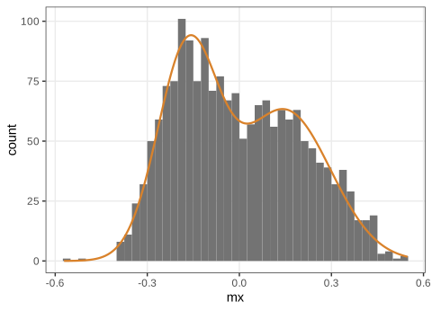
fig_4_28. Reproduces Holmes and Huber (2019), Figure 4.28. Download: PDF · SVG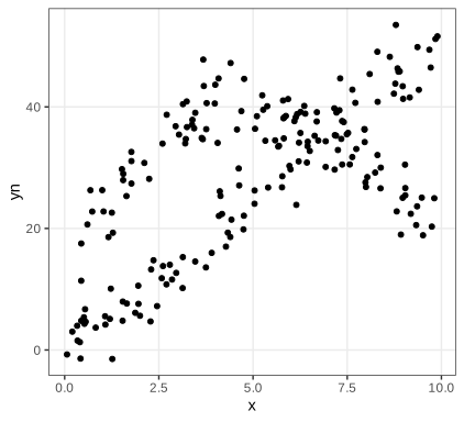
NPreg data of the flexmix package: 200 points from a straight line and a downward parabola. Code: ch04_mixture_models.R, fig_4_29. Reproduces Holmes and Huber (2019), Figure 4.29. Download: PDF · SVG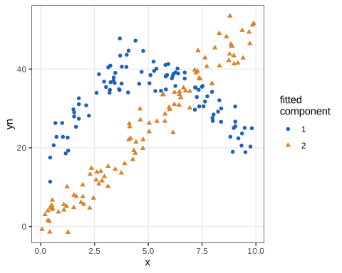
NPreg coloured by the cluster of a two-component mixture of quadratic regressions (flexmix). Near the crossings of line and parabola points cannot be assigned reliably. Code: ch04_mixture_models.R, fig_4_30. Reproduces Holmes and Huber (2019), Figure 4.30. Download: PDF · SVGCorrections to the book
Places where the text, an equation or the code of the book's Chapter 4 is wrong or inconsistent, with the evidence. Each is also discussed where it occurs.
- (4.4). The book: complete-data likelihood \(\prod_{u_i=1}\phi_1(x_i)\prod_{u_i=2}\phi_2(x_i)\). Correct: the factors \(\lambda\) and \(1-\lambda\) are missing; without them \(\lambda\) cannot be estimated from (4.4). Evidence: Section 4.2.2.
- (4.7). The book: \(\prod_i\sum_up(x_i,u\given\theta)\,w(x_i,u\given\theta)\). Correct: \(\prod_i\sum_up(x_i,u\given\theta)\), no weight. Evidence: Gap 4.3: 91.78 versus 417.22 on the Exercise 4.1 data.
- (4.11). The book: \(\hat F_n(x)=\frac1n\sum\ind_{x\le x_i}\). Correct: \(\frac1n\sum\ind\{x_i\le x\}\). Evidence: Definition 4.3; agreement with
ecdf. - Section 4.3. The book: \(\bar x=\int\delta_{x_i}(x)\,\d x\). Correct: \(\bar x=\int t\,\d\hat F_n(t)\)
\({}=\frac1n\sum x_i\). Evidence: Gap 4.10. - Figure 4.15 caption. The book: the median absolute deviation is the Laplace scale \(\phi\). Correct: the MLE of \(\phi\) is the mean absolute deviation from the median; the median absolute deviation estimates \(\phi\log2\). Evidence: Gap 4.13: 0.710 and 0.489 for \(\phi=0.707\).
- Section 4.4.1. The book: conditional law \(N(\theta+w\mu,\sigma w)\). Correct: variance \(\sigma^2w\) (standard deviation \(\sigma\sqrt w\), as in the book's code). Evidence: Result 4.9.
- After (4.15). The book: mean \(\mu=pa/(1-p)\). Correct: \(\mu=a(1-p)/p\). Evidence: Correction box: 15 versus 6.67.
- Figure 4.23 code. The book: gamma shape 80 (comment says 83.3); bottom panel
size = mu^2/vtot. Correct: shape \(\mu^2/v_1=83.3\); size \(\mu^2/v_1\), so that the gamma-Poisson variance is \(50+30=80\). Evidence: the book's size gives variance 130. - Figure 4.24 caption. The book: "eight different choices" of \(\lambda\). Correct: ten (\(\lambda=10,20,\dots,100\)). Evidence: the book's code.
- (4.18). The book: typeset over two lines so that the factor \(\var X_i\) seems to belong to a separate equation. Correct: \(\var g(X_i)\approx g'(\mu_i)^2\var X_i\)
\({}=g'(\mu_i)^2v(\mu_i)\). Evidence: Result 4.11. - Figure 4.26 code. The book:
cumsum(slopes * mean). Correct: a Riemann sum uses the increments of the means; the book's version is proportional to it only because the means double. Evidence: Gap 4.17.
Demonstrations for this chapter
Each demonstration runs in the browser with seeded random numbers, uses the chapter's data where possible, and reproduces the numbers of the course's R code (the R values are shown next to the page's own).
| Demonstration | What you can see | Sections and results |
|---|---|---|
| EM for a mixture of two normals, step by step | E and M steps one at a time on the Exercise 4.1 data, with the membership weights and the log-likelihood trace. Presets: 1 quartile start (Fig. 4.28); 2 random membership weights; 3 identical components: a saddle point; 4 overlapping components (Fig. 4.5); 5 Question 4.7. | 4.2.2, Gap 4.4, Gap 4.6, Result 4.3, Gap 4.7, Exercise 4.1 |
| Zero-inflated counts: ChIP-Seq bins and the EM algorithm | Poisson, zero-inflated Poisson (by EM), negative binomial and zero-inflated negative binomial fits to 256,523 bins, on a count, log or rootogram scale. Presets: 1 Poisson (Figs 4.8, 4.9); 2 ZIP by EM; 3 negative binomial; 4 ZINB rootogram; 5 simulated ZIP data. | 4.2.3, Result 4.4, Gap 4.8, Algorithm 4.2 |
| The nonparametric bootstrap on Darwin's Zea mays data | Resampling the 15 differences, the bootstrap distribution of the median, mean or trimmed mean, percentile intervals, and the exact bootstrap distribution of the median. Presets: 1 median, \(B=1000\) (Fig. 4.14); 2 99% interval (Question 4.12); 3 the mean (Question 4.13); 4 Monte Carlo error, \(B=50\); 5 \(B=20000\) against the exact distribution. | 4.3, Gap 4.11, Result 4.6, Result 4.7 |
| Gamma-Poisson counts and variance-stabilising transformations | The gamma rate, the resulting count distribution, and the exact standard deviation of raw, square-root, log and arcsinh-transformed counts against the mean, with delta-method predictions. Presets: 1 Poisson and the square root (Fig. 4.24); 2 gamma-Poisson raw counts (Fig. 4.25); 3 the square root is not enough; 4 log(x + 1); 5 the arcsinh transformation (4.22). | 4.4.3, Result 4.10, 4.4.4, Result 4.11, Gap 4.16, Gap 4.18 |
The R code that produces every figure of this page is code/ch04_mixture_models.R (see the code index).
References
- Holmes, S. and Huber, W. (2019). Modern Statistics for Modern Biology. Cambridge University Press. Chapter 4.
- Andrews, D. F. and Mallows, C. L. (1974). Scale mixtures of normal distributions. Journal of the Royal Statistical Society: Series B, 36(1), 99–102. doi:10.1111/j.2517-6161.1974.tb00989.x.
- Anscombe, F. J. (1948). The transformation of Poisson, binomial and negative-binomial data. Biometrika, 35(3/4), 246–254. doi:10.1093/biomet/35.3-4.246.
- Bickel, P. J. and Freedman, D. A. (1981). Some asymptotic theory for the bootstrap. The Annals of Statistics, 9(6), 1196–1217. doi:10.1214/aos/1176345637.
- Chen, M., Xie, Y. and Story, M. (2011). An exponential-gamma convolution model for background correction of Illumina BeadArray data. Communications in Statistics: Theory and Methods, 40(17), 3055–3069.
- Dempster, A. P., Laird, N. M. and Rubin, D. B. (1977). Maximum likelihood from incomplete data via the EM algorithm. Journal of the Royal Statistical Society: Series B, 39(1), 1–38. doi:10.1111/j.2517-6161.1977.tb01600.x.
- Dvoretzky, A., Kiefer, J. and Wolfowitz, J. (1956). Asymptotic minimax character of the sample distribution function and of the classical multinomial estimator. The Annals of Mathematical Statistics, 27(3), 642–669. doi:10.1214/aoms/1177728174.
- Efron, B. (1979). Bootstrap methods: another look at the jackknife. The Annals of Statistics, 7(1), 1–26. doi:10.1214/aos/1176344552.
- Efron, B. and Tibshirani, R. J. (1993). An Introduction to the Bootstrap. Chapman and Hall/CRC, New York.
- Kiefer, J. and Wolfowitz, J. (1956). Consistency of the maximum likelihood estimator in the presence of infinitely many incidental parameters. The Annals of Mathematical Statistics, 27(4), 887–906.
- Kuan, P. F., Chung, D., Pan, G., Thomson, J. A., Stewart, R. and Keleş, S. (2011). A statistical framework for the analysis of ChIP-Seq data. Journal of the American Statistical Association, 106(495), 891–903.
- Lambert, D. (1992). Zero-inflated Poisson regression, with an application to defects in manufacturing. Technometrics, 34(1), 1–14. doi:10.2307/1269547.
- Lange, K. (2016). MM Optimization Algorithms. SIAM, Philadelphia.
- Leisch, F. (2004). FlexMix: a general framework for finite mixture models and latent class regression in R. Journal of Statistical Software, 11(8), 1–18. doi:10.18637/jss.v011.i08.
- Massart, P. (1990). The tight constant in the Dvoretzky-Kiefer-Wolfowitz inequality. The Annals of Probability, 18(3), 1269–1283. doi:10.1214/aop/1176990746.
- McLachlan, G. and Peel, D. (2000). Finite Mixture Models. Wiley, New York.
- Singh, K. (1981). On the asymptotic accuracy of Efron's bootstrap. The Annals of Statistics, 9(6), 1187–1195. doi:10.1214/aos/1176345636.
- Teicher, H. (1963). Identifiability of finite mixtures. The Annals of Mathematical Statistics, 34(4), 1265–1269. doi:10.1214/aoms/1177703862.
- Tibshirani, R. (1996). Regression shrinkage and selection via the lasso. Journal of the Royal Statistical Society: Series B, 58(1), 267–288. doi:10.1111/j.2517-6161.1996.tb02080.x.
- Wills, Q. F., Livak, K. J., Tipping, A. J. et al. (2013). Single-cell gene expression analysis reveals genetic associations masked in whole-tissue experiments. Nature Biotechnology, 31(8), 748–752.
- Wu, C. F. J. (1983). On the convergence properties of the EM algorithm. The Annals of Statistics, 11(1), 95–103. doi:10.1214/aos/1176346060.
The numerical statements in the text (EM estimates and iteration counts, the zero-inflated and negative binomial fits, exact bootstrap quantities, Laplace and gamma-Poisson identities, exact standard deviations of transformed counts) come from the course's R code.