Random Forests
Bagging averages many trees grown on bootstrap samples, but trees grown from the same data resemble each other, and an average of correlated quantities keeps a floor of variance that no number of trees removes. A random forest lowers that floor by letting each split choose among only a few randomly drawn inputs. This chapter derives the variance formula behind the idea, shows that the out-of-bag error is leave-one-out cross-validation obtained for free, explains what the Gini and permutation importances measure and how proximities give a picture of the data, proves that adding trees cannot cause overfitting, and decomposes the error of a forest into the correlation between trees, the variance of one tree and the bias, which together decide the best number of candidate inputs.
Ch. 1 Introduction Ch. 2 Supervised learning Ch. 3 Linear regression Ch. 4 Linear classification Ch. 5 Basis expansions Ch. 6 Kernel smoothing Ch. 7 Model assessment Ch. 8 Inference and averaging Ch. 9 Additive models and trees Ch. 10 Boosting Ch. 11 Neural networks Ch. 12 SVMs Ch. 13 Nearest neighbours Ch. 14 Unsupervised learning Ch. 15 Random forests Ch. 16 Ensembles Ch. 17 Graphical models Ch. 18 High-dimensional problems
How to read these notes
They follow the book. Sections carry the book's numbers (15.2, 15.4.1, ...) and every displayed equation that appears in the book carries the book's own equation number, e.g. \((15.1)\). Equations without a number are steps that the book skips.
Filling the gaps. Wherever the book states a property without proof or leaves it to an exercise, an orange Filling the gap box or a proof gives the full argument. Proofs and derivations start hidden: open one with its bar, or use the button below.
Figures and demonstrations. All eleven figures of the chapter are computed, and all are reproduced from scratch by the Python code (Algorithm 15.1 is implemented there, and its trees agree with a standard library's), at a scale that runs on a laptop; two supplementary figures cover Exercise 15.6 and Section 15.4.3. The ▶ Demo boxes open an interactive demonstration already set to the case being discussed.
Main reference
T. Hastie, R. Tibshirani and J. Friedman, The Elements of Statistical Learning: Data Mining, Inference, and Prediction, 2nd edition, Springer (2009), Chapter 15, pages 587–604 (book website, with the data sets: hastie.su.domains/ElemStatLearn). Section, equation, figure and exercise numbers below refer to this book. Further reading is listed in the references.
The explanations, derivations, figures and code are my own; equations are cited by their numbers in the book.
Companion courses
Parts of this chapter also appear in the two companion courses on this site. The overlapping material is:
- Section 15.2, the variance of an average of correlated predictors (15.1) and why bagged models stay correlated: Bayesian and Probabilistic Machine Learning, Section 14.2, with Algorithm 14.1 (bagging), Result 14.2 (committee error for arbitrary errors) and Filling the gap 14.3 (the error shared by all bootstrap members).
- Regression and classification trees: Section 14.4 of the same course.
- Model averaging, the \(1/M\) result and its limits: Foundations of Deep Learning, Section 9.6 and Result 9.11.
Where a proof there is the same, these notes state the result, sketch the argument and link to it. New here: the random selection of split variables and the exact decomposition of the correlation between trees, out-of-bag estimation and its limit, the two importance measures, proximities, the behaviour as trees are added, bias, and the nearest-neighbour view. The companion course's trees and committees demo shows bagged regression trees in one dimension; the demonstrations here are different (the correlation–variance trade-off in \(m\), out-of-bag error, importance on real data).
The chapter at a glance
- 15.2 A random forest (Algorithm 15.1) is bagging in which each split may use only \(m\) of the \(p\) inputs, drawn afresh at every node. An average of \(B\) trees with variance \(\sigma^2\) and pairwise correlation \(\rho\) has variance \(\rho\sigma^2+(1-\rho)\sigma^2/B\) (Result 15.1), so lowering \(\rho\) is the only way to reduce variance beyond what more trees give. Spam data: forest 4.7%, bagging 5.3%, boosting 4.4% test error.
- 15.3 Each case is out of bag for about 37% of the trees; voting with those trees estimates the test error, and with many trees this is exactly leave-one-out cross-validation (Result 15.2). Gini importance for two classes is twice a reduction in squared error (Filling the gap 15.4); permutation importance in a linear model is \(2\hat\beta_j^2\) (Result 15.3). Proximities define a Euclidean embedding (Result 15.4). Adding trees never hurts in squared error (Result 15.5), but deep trees can overfit.
- 15.4 The variance of the forest is \(\rho(x)\sigma^2(x)\) and \(\rho(x)\) is the share of the between-training-set variance in the variance of one tree (Result 15.6, Exercise 15.5). The forest has the bias of one randomised tree, and a single randomised tree's error exceeds the forest's by exactly the within-training-set variance (Result 15.7). A forest is a weighted nearest-neighbour rule with data-driven weights (Result 15.8).
Notation. Training data \(\bZ=\{z_i=(x_i,y_i)\}_{i=1}^N\), \(x_i\in\R^p\). A tree grown with random choices \(\Theta\) (the bootstrap sample and the variables offered at each split) is \(T(x;\Theta)\); \(\Theta_1,\Theta_2,\dots\) are independent draws given \(\bZ\). \(\E_{\Theta|\bZ}\) and \(\Var_{\Theta|\bZ}\) average over \(\Theta\) with the data fixed; \(\E_{\bZ}\), \(\Var_{\bZ}\) over training sets.
Prerequisites. Trees (Section 9.2), bagging (Section 8.7), boosting and relative importance (Section 10.13.1), cross-validation and the bootstrap (Sections 7.10–7.11).
15.1 Introduction
p. 587 Bagging (Section 8.7) fits the same procedure to many bootstrap samples and averages the fits (regression) or lets them vote (classification). It reduces variance, and it helps most for procedures with high variance and low bias, such as large trees. Boosting (Chapter 10) also combines many trees, but each one is fitted to what the previous ones got wrong, so the members are not exchangeable and the method attacks bias as well. Random forests (Breiman, 2001) keep the exchangeable, averaged structure of bagging but make the trees less alike. On many problems they come close to boosting while needing almost no tuning.
See also (this course): Result 8.12 (averaging cannot increase squared error) and Result 8.13 (when voting helps under 0–1 loss); the bagging demo.
15.2 Definition of Random Forests
pp. 587–592 Trees suit averaging: grown deep, they can represent complicated interactions and have small bias, but they are notoriously unstable. Because the bootstrap trees of bagging are identically distributed, the expectation of their average equals the expectation of any one of them: averaging leaves the bias alone and can only act on the variance.
Algorithm 15.1 (random forest for regression or classification) p. 588
- For \(b=1,\dots,B\):
- draw a bootstrap sample \(\bZ^*\) of size \(N\) from the training data;
- grow a tree \(T_b\) on \(\bZ^*\), splitting every node until the minimum node size \(n_{\min}\) is reached, where each split is found as follows:
- draw \(m\) of the \(p\) variables at random;
- find the best split variable and split point among these \(m\);
- split the node into two daughter nodes.
- Output the ensemble \(\{T_b\}_1^B\).
Prediction at \(x\): for regression \(\hf^B_{\rm rf}(x)=\frac1B\sum_{b=1}^BT_b(x)\); for classification \(\hat C^B_{\rm rf}(x)\) is the majority vote of the trees' class predictions \(\hat C_b(x)\).
In our code (grow_tree), the variables are visited in a random order and the best split among the first \(m\) that vary within the node is taken, as in common software; a node is split if it holds more than \(n_{\min}\) cases and is not pure. With \(m=p\) this is bagging, and our trees then reproduce the fitted values of a standard library's trees on the same bootstrap sample.
Result 15.1 (variance of an average of identically distributed, correlated variables; Exercise 15.1) p. 588, (15.1)
Let \(T_1,\dots,T_B\) have common variance \(\sigma^2\) and common pairwise correlation \(\rho\). Then
\[ \Var\Big(\frac1B\sum_{b=1}^BT_b\Big)=\rho\sigma^2+\frac{1-\rho}{B}\sigma^2. \tag{15.1} \]Moreover \(\rho\ge-1/(B-1)\) necessarily, and every \(\rho\in[-1/(B-1),1]\) is possible.
Proof
The variance of a sum is the sum of all entries of the covariance matrix \(\Sigma\), whose \(B\) diagonal entries are \(\sigma^2\) and whose \(B(B-1)\) off-diagonal entries are \(\rho\sigma^2\):
\[ \Var\Big(\sum_bT_b\Big)=\bone^\T\Sigma\bone=B\sigma^2+B(B-1)\rho\sigma^2 . \]Divide by \(B^2\): \(\sigma^2/B+(1-1/B)\rho\sigma^2=\rho\sigma^2+(1-\rho)\sigma^2/B\).
Negative \(\rho\). For \(\rho\lt0\) the formula seems to promise a variance below \(\sigma^2/B\), and even a negative one: \(\rho\sigma^2+(1-\rho)\sigma^2/B\lt0\) when \(\rho\lt-1/(B-1)\). The resolution is that such \(\rho\) cannot occur. Write \(\Sigma=\sigma^2[(1-\rho)I+\rho\bone\bone^\T]\). Its eigenvalues are \(\sigma^2(1-\rho)\) (on vectors orthogonal to \(\bone\), multiplicity \(B-1\)) and \(\sigma^2(1-\rho+B\rho)\) (on \(\bone\)). A covariance matrix is positive semidefinite, so \(1+(B-1)\rho\ge0\), that is \(\rho\ge-1/(B-1)\); conversely, for \(\rho\) in \([-1/(B-1),1]\) both eigenvalues are non-negative and a Gaussian vector with this covariance exists. At the boundary \(\rho=-1/(B-1)\) the sum has variance zero (the \(T_b\) add up to a constant). So for a fixed \(\rho\lt0\) the formula is only valid for \(B\le1-1/\rho\); a negative common correlation cannot be kept up among many variables, and as \(B\to\infty\) an exchangeable correlation must be non-negative. ∎
As \(B\) grows the second term disappears but the first stays: the correlation between bagged trees limits what averaging can achieve. Random forests attack \(\rho\) directly: before each split, only \(m\le p\) randomly chosen inputs are candidates (typical values \(m=\lfloor\sqrt p\rfloor\), or even \(m=1\)). After \(B\) trees \(T(x;\Theta_b)\) are grown, the regression forest predicts
\[ \hf^B_{\rm rf}(x)=\frac1B\sum_{b=1}^BT(x;\Theta_b), \tag{15.2} \]where \(\Theta_b\) records the random choices of tree \(b\) (as in Section 10.9, it determines the split variables, split points and leaf values). Intuitively, smaller \(m\) makes any two trees less alike and so, by (15.1), the average less variable.
See also (companion courses): Result 14.2 of Bayesian and Probabilistic Machine Learning (the same formula for committee errors, with the ambiguity decomposition) and Result 9.11 of Foundations of Deep Learning (the \(1/M\) result and why it fails in practice).
Filling the gap 15.1: why trees from the same data are correlated, and why random split variables decorrelate them pp. 588–589
"Correlation between trees" means correlation over repeated training sets: two trees grown on the same \(\bZ\) share every feature of \(\bZ\). Conditional on \(\bZ\) the trees are independent, so their whole covariance comes from \(\bZ\):
\[ \Cov\big(T(x;\Theta_1),T(x;\Theta_2)\big)=\Var_{\bZ}\,\E_{\Theta|\bZ}T(x;\Theta),\qquad \rho(x)=\frac{\Var_{\bZ}\E_{\Theta|\bZ}T}{\Var_{\bZ}\E_{\Theta|\bZ}T+\E_{\bZ}\Var_{\Theta|\bZ}T}. \]Randomising the split variables adds randomness that is not shared between trees: it raises the within-data part \(\E_{\bZ}\Var_{\Theta|\bZ}T\) and lowers the shared part \(\Var_{\bZ}\E_{\Theta|\bZ}T\) (averaging over many possible split variables smooths the ideal forest), so the ratio falls.
Derivation
By the law of total covariance,
\[ \Cov(T_1,T_2)=\E_{\bZ}\Cov(T_1,T_2\given\bZ)+\Cov_{\bZ}\big(\E[T_1\given\bZ],\E[T_2\given\bZ]\big). \]Given \(\bZ\), \(\Theta_1\) and \(\Theta_2\) are independent (fresh bootstrap draws and fresh variable draws), so the first term is zero; the two conditional means are the same function \(\frf(x)=\E_{\Theta|\bZ}T(x;\Theta)\) of \(\bZ\), so the second is \(\Var_{\bZ}\frf(x)\). The variance of one tree is, by the law of total variance, \(\Var_{\bZ}\frf(x)+\E_{\bZ}\Var_{\Theta|\bZ}T(x;\Theta)\) (this is (15.9) below). Dividing gives the formula, which is Exercise 15.5 and is proved again in Result 15.6.
Why the shared part falls: with \(m=p\) every bootstrap tree on a given \(\bZ\) chooses its splits greedily among the same strongest inputs, so \(\frf\) is a stable, data-specific function and moves a lot from one \(\bZ\) to another. With small \(m\), \(\frf\) is an average over many different tree structures and is much smoother in \(\bZ\). In the simulation of Section 15.4 (Figure 15.10) the shared part drops from 0.134 at \(m=50\) to 0.033 at \(m=1\) while the variance of one tree changes by less than 10%. The same decomposition for bagging is Filling the gap 14.3 of the companion course. ∎
Spam data. Figure 15.1 compares bagging, a random forest and gradient boosting on the spam data of Section 10.8 (the book's split: 3065 training and 1536 test e-mails, 57 inputs).
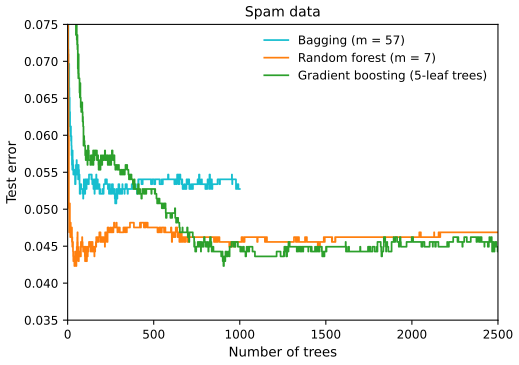
fig_15_1. Reproduces Hastie, Tibshirani and Friedman (2009), Figure 15.1. Download: PDF · SVGThe book reports that bagging is significantly worse than both the forest and boosting by McNemar's test (Exercise 10.6). With our fits the discordant counts (cases one method gets right and the other wrong) are 8 against 17 for bagging against the forest (\(\chi^2_1=3.24\), \(p=0.07\)), 16 against 29 for bagging against boosting (\(\chi^2_1=3.76\), \(p=0.053\)) and 13 against 17 for the forest against boosting (\(p=0.47\)): the same ordering, at the edge of significance. A standard R implementation of the forest with 500 trees gives 4.88% on this split, the book's number; our 500-tree forest gives 4.75%, within the run-to-run variation of one or two test e-mails.
Nested spheres. Figure 15.2 repeats the comparison on the simulation (10.2) of Section 10.1, whose Bayes boundary is a sphere in \(\R^{10}\), an additive function of the squared inputs.
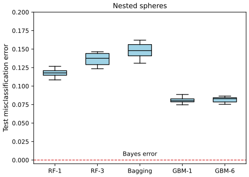
fig_15_2. Reproduces Hastie, Tibshirani and Friedman (2009), Figure 15.2. Download: PDF · SVGBoosting wins clearly, and smaller \(m\) is better, perhaps because the true boundary is additive. Our forests match the book (about 0.12, 0.14 and 0.15); our boosted models are at about 8% where the book shows 5–6%. The difference is the subsampling of the software the book used, which by default grows each tree on a random half of the data (stochastic gradient boosting, Section 10.12.2): in a separate run on one training set, half-sampling brought boosted stumps from 7.8% to 6.0% at 2000 trees.
California housing. Figure 15.3 is a regression comparison on the California housing data of Section 10.14.1.
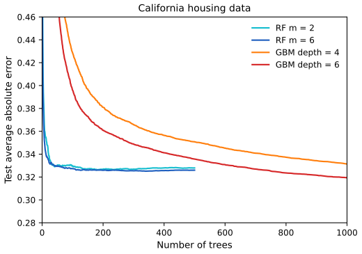
fig_15_3. Reproduces Hastie, Tibshirani and Friedman (2009), Figure 15.3. Download: PDF · SVGTwo of the book's observations hold: the forests settle within 200 trees (0.327 at 200 trees for \(m=2\)) while boosting, slowed down by shrinkage and small trees, is still improving at 1000. The other two hold only partly here. Depth-6 boosting beats both forests, but depth-4 boosting at 1000 trees is still slightly worse than the forest with \(m=6\) (a Wilcoxon signed-rank test on the paired absolute errors gives \(p=2\times10^{-6}\), in favour of the forest; the book finds the reverse with \(p=0.007\)); and \(m=6\) is only marginally better than the default \(m=\lfloor 8/3\rfloor=2\). Our data are a different random split, and the boosting differs in loss and software, so the ranking of close competitors can change.
Linear statistics. Not every estimator gains from this kind of perturbation. Bagging does not change a linear statistic such as the sample mean at all, and two bootstrap means have correlation \(n/(2n-1)\approx\frac12\) (Exercise 15.4); bootstrap trees are much less correlated (\(\rho\le0.07\) in Figure 15.9), which is why trees benefit.
15.3 Details of Random Forests
pp. 592–596 For classification each tree votes and the forest takes the majority (as in bagging, Section 8.7); for regression the trees' predictions are averaged as in (15.2). The inventors recommend \(m=\lfloor\sqrt p\rfloor\) and minimum node size 1 for classification, and \(m=\lfloor p/3\rfloor\) and minimum node size 5 for regression. Both are tuning parameters; Exercise 15.6 (Figure 15.S1) shows how much \(m\) matters on the spam data.
15.3.1 Out of Bag Samples
pp. 592–593 For each case \(z_i=(x_i,y_i)\), the out-of-bag (OOB) predictor averages (or takes the vote of) only the trees whose bootstrap samples do not contain \(z_i\). Its error over the training cases is the OOB error estimate.
Filling the gap 15.2: how many trees are out of bag for a case, and what they were grown on p. 593
A case is missing from a bootstrap sample with probability \((1-1/N)^N\to e^{-1}=0.368\), independently across trees, so after \(B\) trees it has a Binomial\((B,(1-1/N)^N)\) number of OOB trees, about \(0.37B\). Given that case \(i\) is out of bag, the bootstrap sample is a bootstrap sample of size \(N\) from the other \(N-1\) cases.
Derivation
The \(N\) draws are independent and each misses \(i\) with probability \(1-1/N\); trees use independent draws. Since \(N\log(1-1/N)=-1-1/(2N)-\dots\), \((1-1/N)^N\to e^{-1}\) (it is 0.3678 for the 3065 spam training cases; Result 7.14 derives the complementary 0.632). For the second claim, condition each draw on not being \(i\): \(\Pr(\text{draw}=j\given\text{draw}\ne i)=\frac{1/N}{1-1/N}=\frac1{N-1}\) for \(j\ne i\), and the draws remain independent. So the OOB trees of case \(i\) are exactly random-forest trees grown on resamples of size \(N\) of \(\bZ\setminus\{z_i\}\). (Confirmed numerically: among 20,000 simulated resamples of 10 cases that miss case 1, the other cases appear with frequencies \(1/9\pm0.004\).) ∎
Result 15.2 (the OOB estimate becomes leave-one-out cross-validation; Exercise 15.2) p. 593
Fix the data. As \(B\to\infty\), the OOB prediction of case \(i\) converges almost surely to \(\E\big[T(x_i;\Theta^{(-i)})\big]\), where \(\Theta^{(-i)}\) is a random-forest tree grown on a size-\(N\) resample of \(\bZ\setminus\{z_i\}\): the prediction at \(x_i\) of the infinite forest fitted without case \(i\). Hence the OOB error estimate converges to the \(N\)-fold (leave-one-out) cross-validation estimate of the infinite forest, and in the limit the two are identical, provided that the forest fitted to \(N-1\) cases also draws resamples of size \(N\) (with resamples of size \(N-1\) the two differ by the effect of one case in the resample size, which vanishes as \(N\) grows). For classification the OOB vote proportions converge in the same way, so the OOB class equals the leave-one-out class except possibly at exact ties.
Proof
Let \(O_i\) be the indices of the trees for which \(i\) is out of bag. By Filling the gap 15.2, \(|O_i|\to\infty\) almost surely (it is binomial with success probability \((1-1/N)^N>0\)), and the trees in \(O_i\) are independent and identically distributed copies of \(T(\cdot;\Theta^{(-i)})\), because each tree's resample and variable draws are independent of everything else and, conditionally on missing \(i\), the resample has the stated law. Tree outputs are bounded (they are averages of the \(y\)'s), so the strong law of large numbers gives
\[ \hf_{\oob}(x_i)=\frac{1}{|O_i|}\sum_{b\in O_i}T(x_i;\Theta_b)\ \xrightarrow{\text{a.s.}}\ \E\,T(x_i;\Theta^{(-i)})=\hf^{(-i)}_{\rm rf}(x_i). \]This is the leave-one-out prediction of the limiting forest. The OOB error \(\frac1N\sum_iL(y_i,\hf_{\oob}(x_i))\) is a finite sum of continuous functions of these predictions (for squared error; for absolute error likewise), so it converges to \(\frac1N\sum_iL(y_i,\hf^{(-i)}_{\rm rf}(x_i))\), the \(N\)-fold cross-validation estimate (Section 7.10.1 with \(K=N\)). For classification, the proportion of OOB votes for each class converges to the corresponding probability under \(\Theta^{(-i)}\), and the majority class converges whenever the limiting proportions have a unique maximum. ∎
Numerically, on 25 simulated regression cases with 20,000 trees, the OOB predictions of four cases agree with separately grown leave-one-out forests (4000 trees each) to within 0.006, the Monte Carlo error.
So, unlike most nonlinear methods, a forest is cross-validated while it is being fitted, and one can stop adding trees once the OOB error has settled. Figure 15.4 shows this on the spam data.
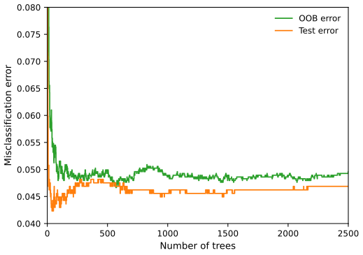
fig_15_4. Reproduces Hastie, Tibshirani and Friedman (2009), Figure 15.4. Download: PDF · SVGThe OOB error after \(b\) trees describes forests of only about \(0.37b\) trees, so for small \(b\) it is biased upward relative to the test error of the \(b\)-tree forest; once both curves are flat this no longer matters.
15.3.2 Variable Importance
pp. 593–594 The first importance measure is the one used for boosted trees (Section 10.13.1): at each split, the improvement in the split criterion is credited to the split variable, and the credits are added up over all splits of all trees.
Filling the gap 15.3: what the Gini importance adds up p. 593
For a node \(t\) with \(n_t\) cases and class proportions \(\hat p_{tk}\), the Gini index is \(G_t=\sum_k\hat p_{tk}(1-\hat p_{tk})\), and a split of \(t\) into \(t_L,t_R\) improves the criterion by \(n_tG_t-n_{t_L}G_{t_L}-n_{t_R}G_{t_R}\ge0\). The Gini importance of input \(j\) is the sum of these improvements over the splits on \(j\), averaged over trees. With two classes, \(n_tG_t=2\sum_{i\in t}(y_i-\bar y_t)^2\) for the 0/1 response, so the Gini importance is exactly twice the squared-error importance (10.43) of the 0/1 response, and a tree grown by the Gini index is the same tree as one grown by least squares on 0/1.
Derivation
With two classes and \(\hat p=\hat p_{t1}\), \(G_t=2\hat p(1-\hat p)\). For the 0/1 response \(\bar y_t=\hat p\) and \(\sum_{i\in t}(y_i-\hat p)^2=n_t\hat p(1-\hat p)\) (the variance of a Bernoulli sample), hence \(n_tG_t=2\sum_{i\in t}(y_i-\bar y_t)^2\). The improvement of a split is therefore twice the drop in residual sum of squares, the two criteria rank all splits identically, and the importances differ by the factor 2. Non-negativity: the residual sum of squares can only fall when a node is split (the children's means are the best constants for the children; Result 9.4). Our implementation confirms both statements split by split. For the two interpretations of the Gini index see Filling the gap 9.6. ∎
The second measure uses the OOB cases. When tree \(b\) has been grown, its accuracy on its OOB cases is recorded; then the values of input \(j\) are randomly permuted among those cases and the accuracy is recorded again. The drop, averaged over trees, is the permutation (randomisation) importance of \(j\). If a tree never splits on \(j\), permuting \(j\) changes none of its predictions, so that tree contributes exactly zero. Permutation removes the information in \(j\) while keeping its marginal distribution, much as setting a coefficient to zero in a linear model, as the next result makes precise.
Result 15.3 (permutation importance in a linear model; Exercise 15.7) p. 604, (15.13)
Fit \(\hat y=x^\T\hat\beta\) by least squares (with an intercept, or without one when all variables are centred) to standardised data: each column has mean 0 and \(\frac1N\sum_ix_{ij}^2=1\). Let \(\RSS\) be the mean squared residual and \(\RSS_j^*\) the same quantity when the \(N\) values of input \(j\) are randomly permuted before predicting with the same \(\hat\beta\). Then
\[ \E_P\big[\RSS_j^*-\RSS\big]=2\hat\beta_j^2, \tag{15.13} \]where \(\E_P\) averages over the \(N!\) permutations. With the other common standardisation \(\frac1{N-1}\sum_ix_{ij}^2=1\), the right side is \(2\hat\beta_j^2(N-1)/N\). On an independent test set the increase is approximately \(2\beta_j^2\Var(X_j)\).
Proof
Let \(r_i=y_i-x_i^\T\hat\beta\) and \(\pi\) a uniformly random permutation. Only coordinate \(j\) changes, so the new residual is \(r_i^*=r_i+\hat\beta_j(x_{ij}-x_{\pi(i)j})\) and
\[ \RSS_j^*-\RSS=\frac2N\hat\beta_j\sum_ir_i(x_{ij}-x_{\pi(i)j})+\frac1N\hat\beta_j^2\sum_i(x_{ij}-x_{\pi(i)j})^2 . \]For each \(i\), \(\pi(i)\) is uniform on \(\{1,\dots,N\}\), so \(\E_P\,x_{\pi(i)j}=\bar x_j=0\). The normal equations give \(\sum_ir_ix_{ij}=0\). Hence the expected first term is 0. For the second,
\[ \E_P\sum_i(x_{ij}-x_{\pi(i)j})^2=2\sum_ix_{ij}^2-2\sum_ix_{ij}\E_P x_{\pi(i)j}=2N. \]Together, \(\E_P[\RSS_j^*-\RSS]=\frac1N\hat\beta_j^2\cdot2N=2\hat\beta_j^2\). With divisor \(N-1\) in the standardisation, \(\sum_ix_{ij}^2=N-1\) and the result is \(2\hat\beta_j^2(N-1)/N\).
Test set. On new data \((x_i,y_i)\), \(i=1,\dots,M\), from the same distribution, independent of the fit, the same expansion holds with test residuals. As \(M\to\infty\), the cross term tends to \(2\hat\beta_j\E[r\,(X_j-X_j')]\) with \(X_j'\) an independent copy, which is \(2\hat\beta_j\Cov(r,X_j)\), small when \(\hat\beta\) is close to the population coefficient (the population residual is uncorrelated with \(X_j\)); and the square term tends to \(\hat\beta_j^2\E(X_j-X_j')^2=2\hat\beta_j^2\Var(X_j)\). So the increase is approximately \(2\hat\beta_j^2\Var(X_j)\). In a simulation with 2000 training and 200,000 test cases we found 1.960 against \(2\hat\beta_1^2=1.917\). ∎
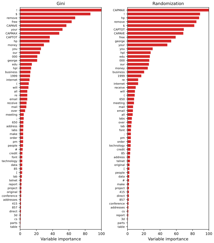
fig_15_5. Reproduces Hastie, Tibshirani and Friedman (2009), Figure 15.5. Download: PDF · SVGThe rankings agree broadly with each other and with boosting (Figure 10.6), but the forest spreads importance over more inputs than boosting does, because random candidate sets give every input chances to be split on. The permutation measure is the more even of the two (median 5.3% of the maximum against 4.4%). Neither measure says what would happen if the input were dropped and the forest refitted: other inputs can then take its place. In the importance demo, refitting without CAPMAX, the input with the largest permutation importance, changes the test error by less than 0.1 percentage points (and the OOB error by 0.3), because CAPAVE and CAPTOT carry nearly the same information (surrogates, Filling the gap 9.8).
Two further properties are worth knowing. The Gini measure credits an input for every split, including the many chance splits deep in fully grown trees, so continuous inputs with many possible split points collect importance even when they carry no information; in our runs a standard-normal noise input added to the spam data received 14% of the largest Gini importance (more than half of the real inputs) but a permutation importance of 0.04 accuracy points, against 3.8 for "!". And two copies of the same input share its Gini importance (each receives about three quarters of the original's, since together they are offered to more splits), whereas permuting one copy still costs nearly as much accuracy as before, because the fitted trees use both.
15.3.3 Proximity Plots
pp. 595–596 While a forest is grown, an \(N\times N\) proximity matrix is accumulated: for every tree, every pair of OOB cases that land in the same leaf has its proximity increased by one. We divide the counts by the number of trees in which both cases were out of bag, so that \(P_{ii}=1\) and \(P_{ik}\) is the fraction of those trees in which \(i\) and \(k\) share a leaf. The matrix is then represented in two dimensions by multidimensional scaling of the dissimilarities \(1-P_{ik}\) (classical scaling, as in common software).
Result 15.4 (proximities are a kernel, and \(1-P\) is a squared Euclidean distance)
Let \(P=\frac1B\sum_bS_b\) with \((S_b)_{ik}=1\) if cases \(i\) and \(k\) fall in the same leaf of tree \(b\) (all cases, not only OOB ones). Then \(P\) is positive semidefinite with unit diagonal, and there are vectors \(\phi_1,\dots,\phi_N\) with \(\|\phi_i-\phi_k\|^2=2(1-P_{ik})\). Hence classical scaling of \(D^2=1-P\) is exact in enough dimensions, and a two-dimensional proximity plot is the best two-dimensional approximation, in the sense of classical scaling, to a genuine Euclidean configuration.
Proof
Index the leaves of tree \(b\) by \(\ell\) and let \(u_{b\ell}\in\{0,1\}^N\) indicate the cases in leaf \(\ell\). Then \(S_b=\sum_\ell u_{b\ell}u_{b\ell}^\T\), a sum of positive semidefinite rank-one matrices, so \(S_b\) and the average \(P\) are positive semidefinite; every case is in exactly one leaf, so the diagonal is 1. Factor \(P=\Phi\Phi^\T\) (for instance \(\Phi=\sqrt{P}\), or the stacked vectors \(B^{-1/2}u_{b\ell}\) read row by row), with rows \(\phi_i\); then \(\|\phi_i-\phi_k\|^2=P_{ii}+P_{kk}-2P_{ik}=2(1-P_{ik})\). Classical scaling of a matrix \(D^2\) of squared Euclidean distances recovers the configuration up to rotation and translation from the eigenvectors of \(-\frac12JD^2J\), \(J=I-\frac1N\bone\bone^\T\), and keeping the two leading eigenvectors gives the best rank-two approximation of that inner-product matrix. On the mixture data, \(-\frac12J(1-P)J\) has smallest eigenvalue \(-8\times10^{-16}\), zero up to rounding. When only OOB pairs are counted and normalised pair by pair, as in Figure 15.6, \(P\) is an average over different sets of trees for different pairs and need not be exactly positive semidefinite; it is close to the all-tree matrix in practice. ∎
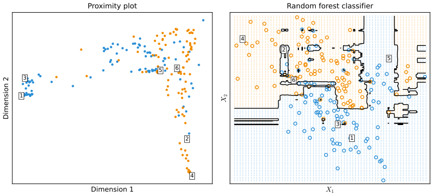
fig_15_6. Reproduces Hastie, Tibshirani and Friedman (2009), Figure 15.6. Download: PDF · SVGProximity plots tend to look alike whatever the data: a star with one arm per class, more pronounced the better the classifier. Mapping points back to the inputs explains why. Two neighbours in a pure region keep sharing leaves, because a pure node is never split again; two close points of different classes near the boundary are separated whenever a tree splits between them, so they share leaves only sometimes, and they end up near the centre where the arms meet.
15.3.4 Random Forests and Overfitting
pp. 596–597 With many inputs of which few are relevant, a small \(m\) can be harmful: at most splits no relevant input may be among the candidates. Figure 15.7 shows this on the model (15.11) of Exercise 15.3 with two relevant inputs.
Filling the gap 15.4: the probabilities printed above Figure 15.7 p. 596
If \(r\) of the \(p\) inputs are relevant and \(m\) are drawn at random without replacement, the number of relevant ones among them is hypergeometric, and
\[ \Pr(\text{at least one relevant candidate})=1-\binom{p-r}{m}\Big/\binom{p}{m}. \]Derivation
All \(\binom pm\) candidate sets are equally likely, and \(\binom{p-r}{m}\) of them contain only irrelevant inputs. With \(r=2\) and \(m=\lfloor\sqrt p\rfloor\): \(p=7,m=2\) gives \(1-10/21=0.524\); \(p=27,m=5\): \(1-\frac{22\cdot21}{27\cdot26}=0.342\); \(p=52,m=7\): 0.253; \(p=102,m=10\): \(1-\frac{92\cdot91}{102\cdot101}=0.187\); \(p=152,m=12\): 0.152. These are the book's 0.52, 0.34, 0.25, 0.19, 0.15. For \(r=6\), \(p=106\), \(m=10\) the formula gives 0.457, the book's 0.46. (In our implementation, as in common software, inputs that are constant within a node are skipped, which matters only in small nodes.) ∎
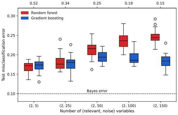
fig_15_7. Reproduces Hastie, Tibshirani and Friedman (2009), Figure 15.7. Download: PDF · SVGAs the probability falls, the gap between the forest and boosting grows. With more relevant inputs the forest is surprisingly robust: with 6 relevant and 100 noise inputs the probability is still 0.46. Part of the reason is that misclassification error is insensitive to the bias and variance of the probability estimates of the individual trees, as long as the vote lands on the right side.
A second claim is that random forests "cannot overfit". That is true of the number of trees: like bagging, the forest (15.2) is a Monte Carlo approximation of the expectation
\[ \frf(x)=\E_\Theta T(x;\Theta)=\lim_{B\to\infty}\hf(x)^B_{\rm rf}, \tag{15.3} \]where the distribution of \(\Theta\) is conditional on the training data.
Result 15.5 (more trees never hurt in squared error) p. 596, (15.3)
Given the data, \(\hf^B_{\rm rf}(x)\to\frf(x)\) almost surely as \(B\to\infty\), and for any target value \(y\)
\[ \E_{\Theta|\bZ}\big[(y-\hf^B_{\rm rf}(x))^2\big]=(y-\frf(x))^2+\frac{\Var_{\Theta|\bZ}T(x;\Theta)}{B}, \]which decreases in \(B\). Hence the expected (over the forest's own randomness) prediction error at every \(x\), and so also the expected test error, can only fall as trees are added, and converges to that of the limit \(\frf\).
Proof
Given \(\bZ\), the trees \(T(x;\Theta_b)\) are independent and identically distributed and bounded, so the strong law of large numbers gives the convergence. Their average has mean \(\frf(x)\) and variance \(\Var_{\Theta|\bZ}T/B\); the identity is the bias–variance decomposition \(\E(y-U)^2=(y-\E U)^2+\Var U\) for \(U=\hf^B_{\rm rf}(x)\). Integrate over test points \((x,y)\) for the test error. For 0–1 loss the expected error need not be monotone in \(B\) (an even number of trees can tie), but it converges, since the vote proportions converge. A simulated check: for a fixed \(\bZ\) and \(B=1,5,25\) the average squared error over forests was 2.858, 1.870, 1.683 against the formula's 2.822, 1.874, 1.685. ∎
The limit itself can overfit, though: an average of fully grown trees can be too rich a model and carry unnecessary variance. Segal (2004) found small gains from limiting the depth of the trees. Figure 15.8 shows a modest effect in a regression example; classifiers are less sensitive to variance, and the effect is rarely seen in classification.
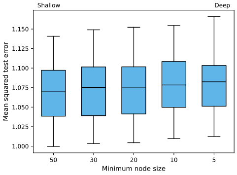
fig_15_8. Reproduces Hastie, Tibshirani and Friedman (2009), Figure 15.8. Download: PDF · SVGIn the authors' experience fully grown trees seldom cost much and save a tuning parameter.
15.4 Analysis of Random Forests
pp. 597–602 We now look at the mechanisms behind the extra randomisation, for regression with squared error (bias and variance under 0–1 loss interact in a more complicated way, Result 7.5). For classification, the forest's average of the trees' class proportions can be studied in the same way as an estimate of the class probabilities.
15.4.1 Variance and the De-Correlation Effect
The limiting forest (15.3), with its dependence on the training data made explicit, is
\[ \frf(x)=\E_{\Theta|\bZ}T(x;\Theta(\bZ)). \tag{15.4} \]Result 15.6 (variance of a forest and the correlation between trees; Exercise 15.5) pp. 597–600, (15.5)–(15.9), (15.12)
At a fixed target point \(x\),
\[ \Var\frf(x)=\rho(x)\sigma^2(x), \tag{15.5} \]where \(\rho(x)\) is the sampling correlation between two trees grown on the same random training set,
\[ \rho(x)=\corr\big[T(x;\Theta_1(\bZ)),T(x;\Theta_2(\bZ))\big], \tag{15.6} \]and \(\sigma^2(x)\) is the sampling variance of one tree,
\[ \sigma^2(x)=\Var\,T(x;\Theta(\bZ)). \tag{15.7} \]The variance of one tree splits into
\[ \Var_{\Theta,\bZ}T(x;\Theta(\bZ))=\Var_{\bZ}\E_{\Theta|\bZ}T(x;\Theta(\bZ))+\E_{\bZ}\Var_{\Theta|\bZ}T(x;\Theta(\bZ)), \tag{15.9} \]total variance = \(\Var_{\bZ}\frf(x)\) + within-\(\bZ\) variance, and therefore
\[ \rho(x)=\frac{\Var_{\bZ}[\E_{\Theta|\bZ}T(x;\Theta(\bZ))]}{\Var_{\bZ}[\E_{\Theta|\bZ}T(x;\Theta(\bZ))]+\E_{\bZ}\Var_{\Theta|\bZ}[T(x;\Theta(\bZ))]}. \tag{15.12} \]The conditional covariance of two trees given \(\bZ\) is zero. For \(B\) trees,
\[ \Var\hf^B_{\rm rf}(x)=\rho(x)\sigma^2(x)+(1-\rho(x))\sigma^2(x)/B, \]which is (15.1) and tends to (15.5).
Proof
(15.9) is the law of total variance for \(T=T(x;\Theta(\bZ))\) conditioned on \(\bZ\). Given \(\bZ\), \(\Theta_1\) and \(\Theta_2\) are independent, so \(\Cov(T_1,T_2\given\bZ)=0\) and, by the law of total covariance,
\[ \Cov(T_1,T_2)=\E_{\bZ}\Cov(T_1,T_2\given\bZ)+\Cov_{\bZ}\big(\E[T_1\given\bZ],\E[T_2\given\bZ]\big)=0+\Var_{\bZ}\frf(x). \]Both trees have variance \(\sigma^2(x)\), given by (15.9), so \(\rho(x)=\Var_{\bZ}\frf(x)/\sigma^2(x)\), which is (15.12) and, rearranged, (15.5). The \(B\) trees of a forest are exchangeable with variance \(\sigma^2(x)\) and pairwise correlation \(\rho(x)\), so Result 15.1 applies. Since \(\Var_{\bZ}\frf\ge0\), \(\rho(x)\ge0\): the case \(\rho\lt0\) of Exercise 15.1 cannot arise for trees. ∎
\(\rho(x)\) is easily confused with the average correlation between the fitted trees of one forest (seeing each tree as the vector of its \(N\) fitted values, given the data). That conditional correlation is not what matters for averaging, and the dependence on \(x\) is a reminder: \(\rho(x)\) is a theoretical correlation at one point, induced by drawing training sets \(\bZ\) from the population and then pairs of trees on each. The variability in (15.6) and (15.7) has both sources: the bootstrap and variable sampling given \(\bZ\), and the sampling of \(\bZ\) itself.
The book's demonstrations use the simulation model
\[ Y=\frac1{\sqrt{50}}\sum_{j=1}^{50}X_j+\varepsilon, \tag{15.8} \]with all \(X_j\) and \(\varepsilon\) independent standard Gaussian, 500 training sets of size 100, and 600 test locations. Trees are nonlinear in \(\bZ\), so the patterns depend somewhat on the model.
Filling the gap 15.5: estimating the quantities of Result 15.6 from a simulation
The book's Figures 15.9 and 15.10 need \(\Var_{\bZ}\frf(x)\), the within-\(\bZ\) variance and the squared bias for the limiting forest, which cannot be grown. With \(R\) training sets and \(B\) trees on each, unbiased estimators exist.
Derivation
At a test point, let \(T_{rb}\) be tree \(b\) on training set \(r\), \(\bar T_r=\frac1B\sum_bT_{rb}\) and \(s^2_r=\frac1{B-1}\sum_b(T_{rb}-\bar T_r)^2\). Write \(V=\Var_{\bZ}\frf\) and \(W=\E_{\bZ}\Var_{\Theta|\bZ}T\).
- Given \(\bZ_r\) the \(T_{rb}\) are i.i.d., so \(\E[s^2_r\given\bZ_r]=\Var_{\Theta|\bZ}T\) and \(\hat W=\frac1R\sum_rs^2_r\) is unbiased for \(W\).
- \(\Var\bar T_r=V+W/B\) (Result 15.6 with \(B\) trees), so with \(S^2=\frac1{R-1}\sum_r(\bar T_r-\bar{\bar T})^2\), \(\hat V=S^2-\hat W/B\) is unbiased for \(V\); then \(\hat\sigma^2=\hat V+\hat W\) and \(\hat\rho=\hat V/\hat\sigma^2\).
- \(\E\bar T_r=\E_{\bZ}\frf\), and \(\E(\mu-\bar{\bar T})^2\)
\({}=(\mu-\E_{\bZ}\frf)^2+\Var\bar T_r/R\), so \(\widehat{\Bias^2}=(\mu-\bar{\bar T})^2-S^2/R\) is unbiased for the squared bias, and the forest's mean squared error (against \(\mu(x)=\E(Y\given x)\)) is estimated by \(\widehat{\Bias^2}+\hat V\). - The variance of the average of the first \(b\) trees has expectation \(V+W/b\), which checks (15.1) directly: in our simulation the simulated values for \(b=1,\dots,10\) agree with \(\hat V+\hat W/b\) to within 1.5% of \(\hat\sigma^2\), for every \(m\).
We used \(R=500\) training sets, \(B=10\) trees per training set and \(m\in\{1,4,7,10,13,19,\)
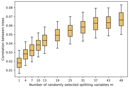
fig_15_9. Reproduces Hastie, Tibshirani and Friedman (2009), Figure 15.9. Download: PDF · SVGPairs of trees grown on different training sets are less alike when they need not use the same split variables, so \(\rho(x)\) falls with \(m\). The variance of one tree (left panel of Figure 15.10, averaged over the test points) hardly changes over most of the range of \(m\), so by (15.5) the forest's variance (right panel) is far below the variance of a tree.
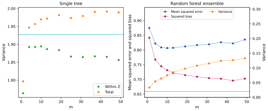
fig_15_10. Reproduces Hastie, Tibshirani and Friedman (2009), Figure 15.10. Download: PDF · SVGNote on the book: does the within-\(\bZ\) variance increase as \(m\) decreases?
The text says that the within-\(\bZ\) variance, the second term of (15.9), increases as \(m\) decreases. That holds from \(m\approx4\) upwards (ours: 1.856 at \(m=50\), 1.894 at \(m=10\)), but at \(m=1\) both the within-\(\bZ\) and the total variance drop sharply (to 1.763 and 1.797), in the book's own Figure 15.10 as in ours. The statement is a trend over most of the range, not a monotone property.
15.4.2 Bias
pp. 600–601 As in bagging, the forest has the bias of one of its randomised trees:
\[ \Bias(x)=\mu(x)-\E_{\bZ}\frf(x)=\mu(x)-\E_{\bZ}\E_{\Theta|\bZ}T(x;\Theta(\bZ)). \tag{15.10} \]Result 15.7 (bias, and what averaging buys) p. 601, (15.10)
A single randomised tree \(T(x;\Theta(\bZ))\) and the forest \(\frf(x)\) have the same bias (15.10). Their mean squared errors against \(\mu(x)\) satisfy
\[ \E\big(T(x;\Theta(\bZ))-\mu(x)\big)^2=\E_{\bZ}\big(\frf(x)-\mu(x)\big)^2+\E_{\bZ}\Var_{\Theta|\bZ}T(x;\Theta(\bZ)): \]the forest improves on one of its trees by exactly the within-\(\bZ\) variance, and in nothing else.
Proof
\(\E T=\E_{\bZ}\E_{\Theta|\bZ}T=\E_{\bZ}\frf\) (tower property), so the biases agree. Each mean squared error is squared bias plus variance; the variances are \(\sigma^2(x)\) and \(\Var_{\bZ}\frf(x)\), whose difference is \(\E_{\bZ}\Var_{\Theta|\bZ}T\) by (15.9). In our simulation the total and forest variances differ by exactly the within-\(\bZ\) estimate at every \(m\), as they must. ∎
The bias of a forest tree is usually larger in absolute value than that of an unpruned tree grown on \(\bZ\), since randomisation and the smaller effective sample restrict it: in Figure 15.10 every forest has squared bias above the 0.659 of a full tree, falling from 0.842 at \(m=1\) to about 0.70 for large \(m\). The improvements of bagging and forests come only from variance reduction, and the choice of \(m\) is a classical bias–variance trade-off.
This resembles ridge regression (Section 3.4.1), which helps when many inputs have similar small coefficients: it shrinks them and lets every input contribute a little. With small \(m\) each relevant input in turn gets to be the main split, and the averaging dilutes the contribution of any single one. Since (15.8) is linear in all inputs, ridge regression does better still.
Filling the gap 15.6: ridge regression on the simulation (15.8) p. 601
The book quotes a mean squared error of about 0.45 with \(\mathrm{df}(\lambda_{\rm opt})\approx29\). On the same 500 training sets as Figure 15.10, ridge regression with an intercept has mean squared error (against \(\mu(x)\), averaged over the 600 test points) at most 0.436, at \(\lambda=50\), where the effective degrees of freedom \(\mathrm{df}(\lambda)=\sum_jd_j^2/(d_j^2+\lambda)\) ((3.50), \(d_j\) the singular values of the centred inputs) average 29.0. This is well below the best forest's 0.807.
Derivation
For each training set, center \(X\) and \(y\), take the SVD \(X_c=UDV^\T\), and form \(\hat\beta_\lambda=V\diag\{d_j/(d_j^2+\lambda)\}U^\T y_c\) for 121 values of \(\lambda\) from 1 to 1000 on a log scale; predict \(\bar y+(x-\bar x)^\T\hat\beta_\lambda\) at the test points, and average \((\hat f_\lambda(x)-\mu(x))^2\) over test points and training sets. Least squares (\(\lambda=0\)) would have error about \(\sigma^2p/(N-p-1)\approx1\) here, since \(p=50\) is half of \(N=100\); shrinking with about 29 degrees of freedom halves it. ∎
15.4.3 Adaptive Nearest Neighbors
pp. 601–602 The forest classifier is close to a weighted nearest-neighbour classifier (Section 13.3 of the book). A fully grown tree's prediction at \(x\) is the response of the one training case in its leaf (or of the few, since pure nodes are not split); the tree-growing has found an informative path to that case. Averaging over trees assigns weights to the training responses, an equivalent kernel concentrated near \(x\).
Result 15.8 (a forest is a weighted average of the training responses)
For a forest whose leaves predict the mean response of their bootstrap cases (regression, or class-1 proportions in classification), the forest's output at \(x\) is
\[ \frac1B\sum_{b=1}^BT_b(x)=\sum_{i=1}^Nw_i(x)\,y_i,\qquad w_i(x)=\frac1B\sum_{b=1}^B\frac{c_{bi}\,I\big(x_i\in L_b(x)\big)}{\sum_kc_{bk}\,I\big(x_k\in L_b(x)\big)}, \]where \(L_b(x)\) is the leaf of tree \(b\) containing \(x\) and \(c_{bi}\) the number of times case \(i\) is in the bootstrap sample of tree \(b\). The weights are non-negative and sum to one; they depend on \(x\) and on the data (including the responses, through the splits), which is why the neighbourhoods are adaptive.
Proof
The leaf value of tree \(b\) at \(x\) is \(\sum_ic_{bi}I(x_i\in L_b(x))y_i\big/\sum_kc_{bk}I(x_k\in L_b(x))\), a weighted mean of the responses with non-negative weights summing to one (the leaf contains at least one bootstrap case). Averaging over \(b\) preserves both properties. Majority voting with pure leaves is the vote of the same weighted average thresholded at \(\tfrac12\). On the mixture data, the weights at \((1.0,0.6)\) reproduce the forest's vote fraction 0.586 exactly, and are spread over 100 training cases with an effective number \(1/\sum_iw_i^2=29.7\) (Figure 15.S2). ∎
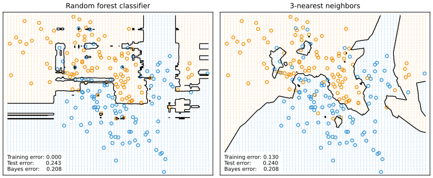
fig_15_11. Reproduces Hastie, Tibshirani and Friedman (2009), Figure 15.11. Download: PDF · SVG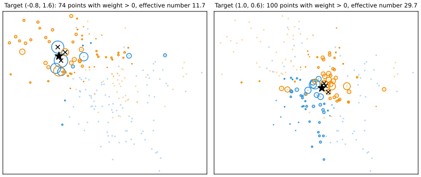
fig_15_s2. Download: PDF · SVGSee also (this course): the \(k\)-nearest-neighbour classifier on the same data, Section 2.3.2.
Bibliographic Notes
pp. 602–603 Random forests in this form are due to Breiman (2001), though related ideas came earlier: Ho (1995) coined the term for trees grown in random subspaces of the inputs; Kleinberg (1990, 1996) used stochastic perturbation and averaging against overfitting; Amit and Geman (1997) grew randomised trees on image features; Breiman (1996) introduced bagging; Dietterich (2000) chose at random among the 20 best splits at each node, and found gains over bagging. Friedman and Hall (2007) showed that subsampling without replacement is an effective alternative to the bootstrap: averaging trees grown on half-samples behaves much like bagging, and smaller fractions decorrelate the trees further.
Exercises
All 7 exercises of Chapter 15 (Hastie, Tibshirani and Friedman, 2009, pp. 603–604), restated in my own words, with complete solutions (hidden).
Exercise 15.1. Derive the variance formula (15.1). It seems to break down for negative \(\rho\); explain what goes wrong.
Solution
See Result 15.1. The variance of the average is
\[ \frac1{B^2}\bone^\T\Sigma\bone=\frac1{B^2}[B\sigma^2+B(B-1)\rho\sigma^2]=\rho\sigma^2+(1-\rho)\sigma^2/B. \]For \(\rho\lt0\) the formula becomes negative once \(B>1-1/\rho\), which is impossible for a variance. The diagnosis: an exchangeable correlation matrix \((1-\rho)I+\rho\bone\bone^\T\) has eigenvalue \(1+(B-1)\rho\) on \(\bone\), so it is a valid correlation matrix only if \(\rho\ge-1/(B-1)\). Negative pairwise correlation cannot be shared equally by many variables; for \(B=2\) any \(\rho\ge-1\) works, for \(B=6\) only \(\rho\ge-0.2\) (numerically, the matrix with \(\rho=-0.22\) has a negative eigenvalue \(-0.1\)). For random-forest trees \(\rho(x)\ge0\) anyway (Result 15.6).
Exercise 15.2. Show that as the number of trees grows, the OOB error estimate of a random forest approaches its \(N\)-fold cross-validation estimate, with equality in the limit.
Solution
See Result 15.2, whose proof uses Filling the gap 15.2: the trees for which case \(i\) is out of bag are, given the data, i.i.d. forest trees grown on resamples of size \(N\) from the other \(N-1\) cases; there are infinitely many of them in the limit, so their average converges to the leave-one-out prediction of the infinite forest, and the OOB error converges to the leave-one-out (\(N\)-fold) cross-validation error. The identity is exact for a cross-validated forest that draws resamples of size \(N\) from the \(N-1\) retained cases; if it draws resamples of size \(N-1\), the two limits differ only through the resample size, a difference that vanishes as \(N\) grows. Confirmed numerically: OOB predictions from 20,000 trees agree with separately grown leave-one-out forests to within the Monte Carlo error.
Exercise 15.3. For the simulation model of Figure 15.7 (Mease and Wyner, 2008), binary responses are generated with
\[ \Pr(Y=1\given X)=q+(1-2q)\cdot I\Big[\sum_{j=1}^JX_j>J/2\Big], \tag{15.11} \]with \(X\) uniform on \([0,1]^p\), \(0\le q\le\frac12\) and an even \(J\le p\). Describe the probability surface and give the Bayes error rate.
Solution
Surface. \(\Pr(Y=1\given x)\) takes only two values: \(1-q\) on the half of the cube above the hyperplane \(x_1+\dots+x_J=J/2\), and \(q\) below it. It depends on the first \(J\) inputs only, through their sum, so it is a step across a diagonal hyperplane (for \(J=2\), the anti-diagonal \(x_1+x_2=1\) of the unit square); the other \(p-J\) inputs are pure noise. The two halves have equal probability, since \(\sum_{j\le J}X_j\) is symmetric about \(J/2\) (replace each \(X_j\) by \(1-X_j\)). The function is not additive in the inputs, and an axis-parallel tree can only approximate the diagonal boundary by a staircase.
Bayes error. The Bayes rule predicts 1 above the hyperplane and 0 below (for \(q\lt\frac12\)); it errs with probability \(\min(q,1-q)=q\) at every \(x\), so the Bayes error is \(q\) (for \(q=\frac12\) every rule has error \(\frac12\)). In Figure 15.7, \(q=0.1\). A simulation with \(J=4\), \(q=0.15\) and 400,000 cases gives 0.1505.
Exercise 15.4. Let \(x_1,\dots,x_n\) be i.i.d. with mean \(\mu\) and variance \(\sigma^2\), and let \(\bar x_1^*\), \(\bar x_2^*\) be the means of two bootstrap samples. Show that \(\corr(\bar x_1^*,\bar x_2^*)=\frac{n}{2n-1}\approx50\%\), deriving \(\Var(\bar x_1^*)\) and the variance of the bagged mean \(\bar x_{\rm bag}\) on the way. (The mean is linear, and bagging does not reduce the variance of linear statistics.)
Solution
Condition on the data \(\bx\). A bootstrap mean is the average of \(n\) independent draws from the empirical distribution, whose mean is \(\bar x\) and variance \(\hat\sigma^2=\frac1n\sum_i(x_i-\bar x)^2\), so
\[ \E[\bar x^*\given\bx]=\bar x,\qquad \Var[\bar x^*\given\bx]=\hat\sigma^2/n. \]Bagged mean. \(\bar x_{\rm bag}=\E[\bar x^*\given\bx]=\bar x\): bagging returns the sample mean itself, with variance \(\sigma^2/n\); nothing is gained.
Variance of one bootstrap mean. By the law of total variance and \(\E\hat\sigma^2=\frac{n-1}n\sigma^2\),
\[ \Var(\bar x_1^*)=\Var(\bar x)+\E\frac{\hat\sigma^2}{n}=\frac{\sigma^2}{n}+\frac{(n-1)\sigma^2}{n^2}=\frac{(2n-1)\sigma^2}{n^2}. \]Covariance. Given \(\bx\) the two bootstrap means are independent, so \(\Cov(\bar x_1^*,\bar x_2^*)\)
\[ \corr(\bar x_1^*,\bar x_2^*)=\frac{\sigma^2/n}{(2n-1)\sigma^2/n^2}=\frac{n}{2n-1}\ \to\ \tfrac12 . \]\({}=\Var(\E[\bar x^*\given\bx])\) \({}=\Var\bar x=\sigma^2/n\). Hence This is (15.12) with \(V=\sigma^2/n\) and \(W=(n-1)\sigma^2/n^2\). By (15.1), an average of \(B\) bootstrap means has variance \(\frac{\sigma^2}n+\frac{(n-1)\sigma^2}{n^2B}\), which decreases to \(\sigma^2/n\), the variance of \(\bar x\): bagging a linear statistic only removes the noise it added. Simulation with \(n=8\): variance 0.522 against 0.527, correlation 0.531 against \(8/15=0.533\); exact enumeration of all \(4^4\) resamples for \(n=4\) confirms \(\bar x_{\rm bag}=\bar x\).
Exercise 15.5. Show that the sampling correlation between two random-forest trees at \(x\) is given by (15.12), whose numerator is \(\Var_{\bZ}\frf(x)\) and whose second denominator term is the expected conditional variance due to the randomisation.
Solution
See Result 15.6. In brief: given \(\bZ\) the two trees are independent, so by the law of total covariance their covariance is \(\Var_{\bZ}\E_{\Theta|\bZ}T=\Var_{\bZ}\frf(x)\); each has variance \(\Var_{\bZ}\frf(x)+\E_{\bZ}\Var_{\Theta|\bZ}T\) by the law of total variance; divide. The expected conditional variance is the variability of a tree caused by the bootstrap and the random choice of split variables for fixed data, which averaging over trees removes.
Exercise 15.6. Fit random forests to the spam data for a range of \(m\) and plot the OOB error and the test error against \(m\).
Solution
We grew forests of 500 trees for \(m\in\{1,2,3,5,7,10,15,25,40,57\}\) on the book's training set (code:
spam_suite,fig_15_s1).\(m\) OOB error test error 1 0.0457 0.0430 2 0.0457 0.0417 3 0.0473 0.0423 5 0.0496 0.0469 7 0.0499 0.0475 10 0.0512 0.0482 15 0.0512 0.0469 25 0.0542 0.0456 40 0.0568 0.0514 57 0.0587 0.0540 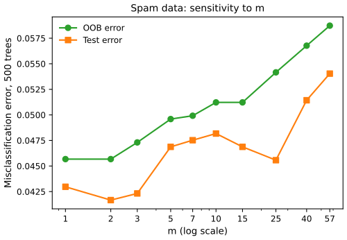
Figure 15.S1 (supplementary, Exercise 15.6). OOB and test error of 500-tree random forests on the spam data against \(m\) (log scale). Code: fig_15_s1. Download: PDF · SVGBoth errors are smallest for small \(m\) (1 to 3) and grow steadily towards bagging (\(m=57\)); the default \(m=7\) is reasonable but not optimal here. The OOB curve follows the test curve's shape and could be used to choose \(m\) without a test set (it picks \(m\le2\), where the test error is also near its minimum); the two curves differ by up to half a percentage point, which is the sampling error of error rates estimated from 3065 and 1536 cases (a standard error of about 0.4 and 0.55 points).
Exercise 15.7. In a linear regression on standardised variables, let \(\RSS\) be the mean squared training residual and \(\RSS_j^*\) the same with the values of input \(j\) randomly permuted before predicting with the same \(\hat\beta\). Show (15.13), \(\E_P[\RSS_j^*-\RSS]=2\hat\beta_j^2\), and argue that it holds approximately on an independent test set.
Solution
See Result 15.3. Expanding the permuted residuals, the cross term has expectation zero (because \(\E_Px_{\pi(i)j}=\bar x_j=0\) and \(\sum_ir_ix_{ij}=0\) by the normal equations), and the square term has expectation \(\frac1N\hat\beta_j^2\cdot2\sum_ix_{ij}^2=2\hat\beta_j^2\) when the standardisation uses the divisor \(N\) (with divisor \(N-1\), the factor is \((N-1)/N\)). On a test set the cross term is approximately zero because the population residual is uncorrelated with \(X_j\), and the square term tends to \(2\hat\beta_j^2\Var(X_j)\). Monte Carlo over 40,000 permutations gave 0.8156 against \(2\hat\beta_1^2=0.8157\). This is why the permutation importance behaves like a squared coefficient: it measures the damage done by destroying the input's information while keeping its distribution, not what a refitted model would lose.
Demonstrations for this chapter
Each demonstration runs in the browser and links back to these notes. The ▶ Demo boxes above open them already set to the case under discussion.
| Demonstration | What you can see | Sections and results |
|---|---|---|
| The correlation–variance trade-off in m | From 500 simulated training sets of the model (15.8) (or a sparse variant): the distribution of \(\rho(x)\) against \(m\), the variance of one tree and its within-training-set part, the forest's squared bias, variance and mean squared error, and the variance of an average of \(b\) trees against \(\rho\sigma^2+(1-\rho)\sigma^2/b\). Presets: 1 bagging; 2 \(m=1\); 3 the best \(m\); 4 only 5 relevant inputs; 5 a forest of 5 trees. | 15.2, 15.4.1, 15.4.2; Results 15.1, 15.6, 15.7; Exercise 15.5 |
| Out-of-bag error against test error | A forest grown tree by tree in the browser on the model (15.11): OOB and test error after each tree, the forest's vote in the plane of the relevant inputs, noise inputs, \(m\), sample size and label noise. Presets: 1 Figure 15.4's message; 2 100 noise inputs; 3 bagging on the same data; 4 few trees; 5 a small sample. | 15.3.1, 15.3.4; Results 15.2, 15.5; Exercises 15.2, 15.3 |
| Gini against permutation importance on the spam data | Both importance measures for forests with \(m=1,3,7,15,57\), with a duplicated input and with noise inputs; rank against rank; the effect of refitting without each of the 12 most important inputs. Presets: 1 Figure 15.5; 2 sorted by permutation; 3 bagging; 4 a copy of "!"; 5 noise inputs. | 15.3.2; Result 15.3, Filling the gap 15.3; Exercises 15.6, 15.7 |
Related demonstrations: in this course, bagging classification trees (Chapter 8) and AdaBoost on the nested spheres (Chapter 10); in the companion course, the trees and committees demo. The Python code that produces every figure of this page is code/ch15_random_forests.py (see the code index).
References
- Hastie, T., Tibshirani, R. and Friedman, J. (2009). The Elements of Statistical Learning: Data Mining, Inference, and Prediction, 2nd edition. Springer, New York. Chapter 15, pp. 587–604. hastie.su.domains/ElemStatLearn.
- Amit, Y. and Geman, D. (1997). Shape quantization and recognition with randomized trees. Neural Computation, 9(7), 1545–1588.
- Breiman, L. (1996). Bagging predictors. Machine Learning, 24(2), 123–140.
- Breiman, L. (2001). Random forests. Machine Learning, 45(1), 5–32.
- Dietterich, T. G. (2000). An experimental comparison of three methods for constructing ensembles of decision trees: bagging, boosting, and randomization. Machine Learning, 40(2), 139–157.
- Friedman, J. H. and Hall, P. (2007). On bagging and nonlinear estimation. Journal of Statistical Planning and Inference, 137(3), 669–683.
- Ho, T. K. (1995). Random decision forests. In Proceedings of the Third International Conference on Document Analysis and Recognition, 278–282.
- Kleinberg, E. M. (1990). Stochastic discrimination. Annals of Mathematics and Artificial Intelligence, 1, 207–239.
- Kleinberg, E. M. (1996). An overtraining-resistant stochastic modeling method for pattern recognition. The Annals of Statistics, 24(6), 2319–2349.
- Lin, Y. and Jeon, Y. (2006). Random forests and adaptive nearest neighbors. Journal of the American Statistical Association, 101(474), 578–590.
- Mease, D. and Wyner, A. (2008). Evidence contrary to the statistical view of boosting (with discussion). Journal of Machine Learning Research, 9, 131–156.
- Segal, M. R. (2004). Machine learning benchmarks and random forest regression. Technical report, Center for Bioinformatics and Molecular Biostatistics, University of California, San Francisco.
The numerical statements in the text (the agreement of our trees with a standard library's, the variance formula and its constraint, the out-of-bag probabilities and the leave-one-out limit, the Gini and permutation identities, the proximity embedding, the decomposition of the simulation into correlation, variance and bias, the ridge comparison, the forest weights, the exercises, and every number quoted from the reproduced figures) were confirmed numerically.