Introduction
Statistical learning means building a rule that predicts an outcome from measured features, using a set of examples in which both are known, and judging the rule by how well it predicts on new cases. The book opens with four data sets that recur throughout: 4601 email messages to be sorted into spam and genuine email, 97 men whose PSA level is to be predicted from clinical measurements, thousands of scanned handwritten digits, and a matrix of 6830 gene expression levels in 64 tumours. These notes reproduce the chapter's displays from the book's own data and use the examples to set up, precisely, the framework that the rest of the course relies on: inputs and outputs, a loss function, the risk and the best possible predictor, and the difference between training error and test error.
Ch. 1 Introduction Ch. 2 Supervised learning Ch. 3 Linear regression Ch. 4 Linear classification Ch. 5 Basis expansions Ch. 6 Kernel smoothing Ch. 7 Model assessment Ch. 8 Inference and averaging Ch. 9 Additive models and trees Ch. 10 Boosting Ch. 11 Neural networks Ch. 12 SVMs Ch. 13 Nearest neighbours Ch. 14 Unsupervised learning Ch. 15 Random forests Ch. 16 Ensembles Ch. 17 Graphical models Ch. 18 High-dimensional problems
How to read these notes
They follow the book. Chapter 1 of the book has no numbered sections, only headings. These notes number them in order: 1.1 is the opening discussion (pages 1–2), 1.2–1.5 are Examples 1–4, and 1.6 collects the closing headings (who should read the book, how it is organized, the website, the note for instructors). Subsections 1.1.1–1.1.4 are additions of these notes: they state the framework that the book develops in Sections 2.2, 2.4 and 7.2, so that every later chapter can refer to it. Where an equation of a later chapter is restated, it carries the book's number, e.g. \((2.9)\).
Filling the gaps. Where the text states something without justification, an orange Filling the gap box or a proof gives the full argument. Proofs and derivations start hidden: open one with its bar, or use the button below.
Figures and demonstrations. All three figures and Table 1.1 are computed from the book's data sets by the Python code. The ▶ Demo boxes open an interactive demonstration already set to the case being discussed.
Main reference
T. Hastie, R. Tibshirani and J. Friedman, The Elements of Statistical Learning: Data Mining, Inference, and Prediction, 2nd edition, Springer (2009), Chapter 1, pages 1–8 (book website, with the data sets: hastie.su.domains/ElemStatLearn). Section, equation, figure and table numbers below refer to this book. Further reading is listed in the references.
The explanations, derivations, figures and code are my own; equations are cited by their numbers in the book.
Companion courses
The framework of this chapter is also developed, from other angles, in the two companion courses on this site:
- Bayesian and Probabilistic Machine Learning (Bishop 2006), Chapter 1: polynomial curve fitting with training and test error (Section 1.1), model selection (Section 1.3), and decision theory (Section 1.5), which proves the minimum-misclassification rule (Result 1.15), the minimum-expected-loss rule (Result 1.16), the reject option (Result 1.17) and the conditional mean as the best predictor under squared loss (Result 1.18).
- Foundations of Deep Learning (Bishop and Bishop 2024), Chapter 1: the kinds of learning (Definition 1.1), a tutorial example with error functions, model complexity and model selection (Section 1.2), and the optimism of the training error for linear smoothers (Result 1.3).
Where a proof there is the same, these notes give a short argument and link to it. New here: the four data sets themselves, the test-set estimate and its standard error, the optimism of k-nearest neighbours, costs for the two kinds of spam error, and the two-way decomposition of the microarray matrix.
The chapter at a glance
- 1.1 Supervised learning predicts an output from inputs using a training set; unsupervised learning describes the structure of inputs alone (Definition 1.1). With a loss function, the best possible predictor is the conditional mean under squared loss (Result 1.1) and the most probable class under 0–1 loss (Result 1.2). A held-out test set estimates the test error without bias, with a standard error (Result 1.3); the training error is too optimistic by \(2\sigma^2\Tr\bS/N\) for a linear smoother (Result 1.4).
- 1.2 Spam: Table 1.1 lists the eleven largest differences in mean word frequency (Filling the gap 1.3); the book's two illustrative rules are a box and a half-plane with error rates of 29% and 35% (Result 1.5); unequal costs move the decision threshold from \(1/2\) to \(c/(1+c)\) (Result 1.6).
- 1.3 Prostate cancer: a regression problem with 8 inputs and 97 men (Figure 1.1); a least-squares line on a 0/1 input joins the two group means (Result 1.7).
- 1.4 Handwritten digits: 256 pixel inputs and 10 classes (Figure 1.2); the “don't know” option is optimal exactly when the largest class probability is below \(1-d\) (Result 1.8).
- 1.5 Microarrays: an unsupervised problem with far more variables than samples (Figure 1.3); for standardised profiles squared distance is \(2p(1-r)\) (Result 1.9); the additive “gene + sample” model explains only 3.4% of the variation (Result 1.10).
Notation. Fixed in Definition 1.2 and used throughout the course: random input \(X\in\R^p\), quantitative output \(Y\in\R\), qualitative output \(G\in\Gc\); observed values \(x_i,y_i,g_i\), \(i=1,\dots,N\); the \(N\times p\) input matrix \(\X\); the training set \(\Tc\).
Prerequisites. Conditional expectation, variance and covariance, and least squares with one input, at the level of a first course in statistics.
1.1 Learning from data
pp. 1–2 The book opens with five prediction tasks: whether a heart-attack patient will have a second attack, the price of a stock in six months, the digits of a handwritten ZIP code, the blood glucose of a diabetic from an infrared spectrum, and the risk factors for prostate cancer. All share one structure. There is an outcome (quantitative, such as a price, or categorical, such as attack/no attack) and a set of features; a training set records both for a collection of objects; from it we build a learner, a rule that predicts the outcome of a new object from its features. A good learner is one that predicts new outcomes accurately, which is a statement about objects not in the training set. This subsection turns these words into definitions.
1.1.1 Supervised and unsupervised learning
Definition 1.1 (supervised and unsupervised learning) p. 2; Sections 2.1–2.2
In supervised learning each object carries an input (feature vector) \(x\) and an output \(y\), and the training data contain both; the goal is a function that predicts the output of a new object from its input. The output “supervises” the learning, in the sense that the training data say what the right answer was. It is called regression when the output is quantitative and classification when it is qualitative (a class label).
In unsupervised learning only inputs are observed. There is no answer to predict; the goal is to describe how the data are organized: groups (clustering), low-dimensional structure, or the dependence between variables. The book treats this in Chapter 14 and, for graphs of dependence, in Chapter 17.
Of the four examples, spam and digits are classification problems, prostate cancer is a regression problem, and the microarray data are best seen as an unsupervised problem (Section 1.5).
See also (companion courses): Foundations of Deep Learning, Definition 1.1 (supervised, unsupervised and self-supervised learning).
1.1.2 Notation
Definition 1.2 (the course's notation) Section 2.2, pp. 9–11
Variables. An input variable is written \(X\); when it is a vector its components are \(X_1,\dots,X_p\). A quantitative output is \(Y\), a qualitative output is \(G\) (for “group”), taking values in a finite set \(\Gc\) of \(K\) classes. Upper case refers to the variable in general (a random variable); lower case to observed values.
Data. The \(i\)th observation is \(x_i\) (a scalar or a \(p\)-vector) with output \(y_i\) or \(g_i\), \(i=1,\dots,N\). The training data are
\[ \Tc=\{(x_1,y_1),\dots,(x_N,y_N)\}\quad\text{or}\quad\{(x_1,g_1),\dots,(x_N,g_N)\}. \]Vectors and matrices. All vectors are columns. Matrices are bold capitals: the inputs form the \(N\times p\) matrix \(\X\) whose \(i\)th row is \(x_i^\T\). A vector is bold only when it has \(N\) components: \(\mathbf{x}_j\in\R^N\) is the \(j\)th column of \(\X\) (all observations of \(X_j\)) and \(\y=(y_1,\dots,y_N)^\T\), while \(x_i\in\R^p\) is not bold.
Predictions. A prediction of \(Y\) is \(\hat Y\), taking values in \(\R\); a prediction of \(G\) is \(\hat G\), taking values in \(\Gc\). A fitted function is written \(\hat f\).
The four examples in this notation:
| Example | Output | Inputs | \(N\) | Type |
|---|---|---|---|---|
| Email spam (1.2) | \(G\in\{\text{email},\text{spam}\}\), \(K=2\) | \(p=57\): 48 word and 6 character frequencies, 3 capital-letter run statistics | 4601 (3065 training, 1536 test) | classification |
| Prostate cancer (1.3) | \(Y=\)lpsa | \(p=8\) clinical measurements | 97 (67 training, 30 test) | regression |
| Digits (1.4) | \(G\in\{0,\dots,9\}\), \(K=10\) | \(p=256\) grey levels | 7291 training, 2007 test | classification |
| Microarrays (1.5) | none | samples as observations: \(p=6830\) genes | 64 | unsupervised |
The last row already shows a feature of modern data: \(p\) can be much larger than \(N\). Chapter 18 of the book is about that case.
1.1.3 Loss, risk and the best possible predictor
“Accurately predicts” needs a measure of error and a population over which to average it. The book's Section 2.4 sets this up; here is the version used throughout the course.
Definition 1.3 (loss function and risk) Section 2.4, (2.9), (2.19)
Let \((X,Y)\) have a joint distribution \(\Pr(X,Y)\). A loss function \(L(y,\hat y)\ge0\) is the price paid for predicting \(\hat y\) when the truth is \(y\). Common choices are the squared error \((y-\hat y)^2\) and the absolute error \(|y-\hat y|\) for a quantitative output, and, for a class label, a \(K\times K\) loss matrix \(\mathbf{L}\) with zero diagonal and nonnegative entries, \(L(k,\ell)\) being the price of classifying an object of class \(k\) as \(\ell\); the 0–1 loss has \(L(k,\ell)=1\) for every \(k\ne\ell\).
The risk, or expected prediction error, of a prediction rule \(f\) is its average loss over the population. For squared error,
\[ \EPE(f)=\E\big(Y-f(X)\big)^2, \tag{2.9} \]and for a classifier \(\hat G\),
\[ \EPE=\E\big[L\big(G,\hat G(X)\big)\big]. \tag{2.19} \]The risk depends on the unknown distribution, so it cannot be computed; but it identifies the target that every method is trying to approach.
Result 1.1 (the regression function is the best predictor under squared loss) Section 2.4, (2.11)–(2.13)
Suppose \(\E Y^2<\infty\) and let
\[ f(x)=\E(Y\given X=x), \tag{2.13} \]the regression function. Then for every function \(g\) with \(\E g(X)^2<\infty\),
\[ \EPE(g)=\EPE(f)+\E\big(g(X)-f(X)\big)^2 . \]So \(f\) minimises (2.9), any other minimiser equals \(f(X)\) with probability one, and the smallest possible risk is \(\EPE(f)=\E\var(Y\given X)\), the part of the variation of \(Y\) that no function of \(X\) can predict. Under absolute error the minimiser is instead the conditional median, \(\operatorname{median}(Y\given X=x)\) (the book's (2.18)).
Proof
Write
\[ Y-g(X)=\{Y-f(X)\}+\{f(X)-g(X)\} \]and expand the square:
\[ \E\big(Y-g(X)\big)^2=\E\big(Y-f(X)\big)^2+2\,\E\big[\{Y-f(X)\}\{f(X)-g(X)\}\big]+\E\big(f(X)-g(X)\big)^2 . \]All three expectations are finite: \(\E f(X)^2\le\E Y^2\) by Jensen's inequality applied to the conditional expectation, and the cross term is bounded by Cauchy–Schwarz. By the tower property, conditioning on \(X\) inside the cross term,
\[ \E\big[\{Y-f(X)\}\{f(X)-g(X)\}\big]=\E\big[\{f(X)-g(X)\}\,\E\{Y-f(X)\given X\}\big]=\E\big[\{f(X)-g(X)\}\cdot0\big]=0, \]because \(f(X)-g(X)\) is a function of \(X\) and \(\E(Y\given X)=f(X)\). This gives the identity. The last term is \(\ge0\), with equality iff \(g(X)=f(X)\) almost surely. Finally
\[ \EPE(f)=\E[\E\{(Y-f(X))^2\given X\}]=\E\var(Y\given X). \]For the median: for fixed \(x\), \(c\mapsto\E(|Y-c|\given X=x)\) is convex with right derivative \(\Pr(Y\le c\given x)-\Pr(Y>c\given x)\), which changes sign at a conditional median. A full treatment of both cases is in the companion course, Result 1.18 and Result 1.19. ∎
Filling the gap 1.1: why it “suffices to minimise pointwise” Section 2.4, (2.11)–(2.12), (2.20)–(2.21)
The book conditions on \(X\), writes \(\EPE(f)=\E_X\E_{Y|X}\big([Y-f(X)]^2\given X\big)\) (2.11), and concludes that \(f(x)\) may be chosen separately at each \(x\) (2.12). Why is this legitimate?
Derivation
Let \(r(x,c)=\E\{L(Y,c)\given X=x\}\) be the conditional risk of predicting the constant \(c\) at \(x\). For any rule \(g\), the tower property gives \(\EPE(g)=\E\,r\big(X,g(X)\big)\). Suppose a rule \(f\) satisfies \(r(x,f(x))\le r(x,c)\) for every \(x\) and every \(c\). Then \(r(X,f(X))\le r(X,g(X))\) for every outcome, and taking expectations, \(\EPE(f)\le\EPE(g)\). Conversely, if \(g\) is worse than \(f\) pointwise on a set of inputs of positive probability, then \(\EPE(g)>\EPE(f)\). Two technical points make this rigorous.
(i) The pointwise minimiser must be a measurable function of \(x\), so that \(f(X)\) is a random variable. For squared loss
\[ r(x,c)=\var(Y\given X=x)+\{\E(Y\given X=x)-c\}^2, \]minimised by the conditional expectation, which exists and is measurable for any \(Y\) with \(\E|Y|<\infty\). For classification
\[ r(x,\ell)=\sum_{k}L(k,\ell)\Pr(G=k\given X=x) \]is a finite list of measurable functions of \(x\); the rule “take the smallest \(\ell\) attaining the minimum” is measurable, being built from finitely many comparisons.
(ii) Ties do not matter: when several classes attain the minimum at \(x\), any choice gives the same conditional risk there, so every tie-breaking rule has the same risk. ∎
Result 1.2 (the Bayes classifier) Section 2.4, (2.20)–(2.23)
Let \(p_k(x)=\Pr(G=k\given X=x)\). With loss matrix \(\mathbf{L}\), the rule
\[ \hat G(x)=\argmin_{g\in\Gc}\sum_{k=1}^KL(k,g)\Pr(G=k\given X=x) \tag{2.21} \]minimises the risk (2.19). With the 0–1 loss it becomes
\[ \hat G(x)=\argmin_{g\in\Gc}\big[1-\Pr(g\given X=x)\big], \tag{2.22} \]that is, \(\hat G(x)=k\) when \(p_k(x)=\max_gp_g(x)\) (2.23): classify to the most probable class. Its risk, the Bayes rate, is \(1-\E\max_kp_k(X)\).
Proof
Conditionally on \(X=x\), predicting \(g\) costs \(\sum_kL(k,g)p_k(x)\) on average (this is (2.20) before the outer expectation). By Filling the gap 1.1 the rule that minimises this at each \(x\) minimises the risk, which is (2.21). For the 0–1 loss
\[ \sum_kL(k,g)p_k(x)=\sum_{k\ne g}p_k(x)=1-p_g(x), \]minimised by the largest \(p_g(x)\); the conditional risk is then \(1-\max_gp_g(x)\), and averaging over \(X\) gives the Bayes rate. The same argument, with figures, is in the companion course: Result 1.15 and Result 1.16. ∎
Results 1.1 and 1.2 describe the ideal, which needs the joint distribution. Every method in the book is a way of estimating \(f\) or the \(p_k\) from a finite training set, and the two simplest, previewed in the prostate demonstration, are a linear model fitted by least squares and the k-nearest-neighbour average \(\hat f(x)=\Ave(y_i\given x_i\in N_k(x))\) (the book's (2.14), Chapter 2).
See also (companion course): Bayesian and Probabilistic Machine Learning, Section 1.5 (decision theory).
1.1.4 Training error and test error
A learner is a map from a training set \(\Tc\) to a fitted rule \(\hat f\). Two different averages of the loss then matter, and confusing them is the most common mistake in the subject. The book's Section 7.2 names them.
Definition 1.4 (training error, test error, expected test error) Section 7.2, (7.2)–(7.4)
Let \(\hat f\) be fitted on \(\Tc\), and let \((X,Y)\) be a new draw from the population, independent of \(\Tc\). The test error (generalisation error) of the fitted rule is
\[ \Err_\Tc=\E\big[L\big(Y,\hat f(X)\big)\given\Tc\big], \tag{7.2} \]its risk with the training set held fixed. Averaging also over training sets gives the expected test error
\[ \Err=\E\big[L\big(Y,\hat f(X)\big)\big]=\E\big[\Err_\Tc\big]. \tag{7.3} \]The training error is the average loss on the data used for fitting:
\[ \err=\frac1N\sum_{i=1}^NL\big(y_i,\hat f(x_i)\big). \tag{7.4} \]The training error is free to compute but answers the wrong question: the fit was chosen to make it small, so it flatters the fit. The honest alternative, when data are plentiful, is to hold out a test set that plays no part in fitting. The prostate and spam data come with such a split.
Result 1.3 (the test-set estimate and its standard error)
Let \((x'_1,y'_1),\dots,(x'_M,y'_M)\) be independent draws from the population, independent of \(\Tc\), and let \(\ell_m=L(y'_m,\hat f(x'_m))\). Given \(\Tc\), the test-set estimate \(\widehat{\Err}=\frac1M\sum_m\ell_m\) satisfies
\[ \E\big[\widehat{\Err}\given\Tc\big]=\Err_\Tc,\qquad \var\big(\widehat{\Err}\given\Tc\big)=\frac{\var(\ell_1\given\Tc)}{M}, \]so it is unbiased for the test error of the rule actually fitted, with standard error estimated by \(s_\ell/\sqrt M\), where \(s_\ell\) is the sample standard deviation of the \(\ell_m\). If the \(\ell_m\) have finite variance, \(\widehat{\Err}\to\Err_\Tc\) as \(M\to\infty\), and \((\widehat{\Err}-\Err_\Tc)/(s_\ell/\sqrt M)\) is approximately standard normal for large \(M\).
Proof
Condition on \(\Tc\); then \(\hat f\) is a fixed function and \(\ell_1,\dots,\ell_M\) are independent and identically distributed, each with conditional mean \(\E[L(Y,\hat f(X))\given\Tc]=\Err_\Tc\) by (7.2). The mean of \(M\) such variables has the same mean and \(1/M\) times the variance. \(s_\ell^2\) is unbiased for \(\var(\ell_1\given\Tc)\), and the law of large numbers and the central limit theorem, applied conditionally on \(\Tc\), give the last two statements. Note what is not estimated: \(\widehat{\Err}\) says nothing about how a fit on a different training set would do, which is \(\Err\) in (7.3). ∎
On the prostate data (\(M=30\) test men), least squares on all eight inputs has \(\widehat{\Err}=0.521\) with standard error \(0.179\), the values of the book's Table 3.3; predicting every man by the training mean gives \(1.057\) (standard error \(0.396\)). A standard error of a third of the estimate is a warning: 30 test cases are few, and differences of a few hundredths between methods on this test set (Table 3.3 compares six) are well inside the noise. Chapter 7 develops cross-validation and the bootstrap for exactly this reason.
Result 1.4 (the optimism of the training error) Section 7.4, (7.18)–(7.24)
Fix the inputs \(x_1,\dots,x_N\) and let \(y_i=f(x_i)+\varepsilon_i\) with independent errors of mean 0 and variance \(\sigma^2\). Let \(\hat y_i=\hat f(x_i)\) be fitted values computed from \(\y\), let \(Y^0_i\) be a new response at \(x_i\), independent of \(\y\), and let \(\Err_{\rm in}=\frac1N\sum_i\E_{Y^0}\big[(Y^0_i-\hat y_i)^2\given\y\big]\) be the in-sample error (7.18). With squared error loss:
(a) \(\displaystyle \E(\Err_{\rm in})-\E(\err)=\frac2N\sum_{i=1}^N\cov(\hat y_i,y_i)\), the book's (7.21)–(7.22);
(b) for a linear smoother \(\hat\y=\bS\y\), with \(\bS\) depending on the inputs only, \(\sum_i\cov(\hat y_i,y_i)=\sigma^2\Tr\bS\);
(c) for least squares with \(d\) linearly independent columns (intercept included), \(\bS=\H=\X(\X^\T\X)^{-1}\X^\T\) and \(\Tr\H=d\), so
\[ \E(\Err_{\rm in})=\E(\err)+2\cdot\frac dN\,\sigma^2 ; \tag{7.24} \](d) for the k-nearest-neighbour average, if every neighbourhood \(N_k(x_i)\) contains \(x_i\) itself and exactly \(k\) points, \(\Tr\bS=N/k\) and the optimism is \(2\sigma^2/k\).
Proof
(a) Write \(f_i=f(x_i)\). Because \(Y^0_i\) has mean \(f_i\), variance \(\sigma^2\) and is independent of \(\hat y_i\),
\[ \E(Y^0_i-\hat y_i)^2=\E(Y^0_i-f_i)^2+\E(f_i-\hat y_i)^2=\sigma^2+\E(f_i-\hat y_i)^2 . \]For the training response the cross term does not vanish:
\[ \E(y_i-\hat y_i)^2=\E(y_i-f_i)^2+\E(f_i-\hat y_i)^2-2\,\E\big[(y_i-f_i)(\hat y_i-f_i)\big]=\sigma^2+\E(f_i-\hat y_i)^2-2\cov(y_i,\hat y_i), \]since \(\E(y_i-f_i)=0\) makes
\[ \E[(y_i-f_i)(\hat y_i-f_i)]=\E[(y_i-f_i)\hat y_i]=\cov(y_i,\hat y_i). \]Subtracting and averaging over \(i\) gives (a).
(b)
\[ \cov(\hat y_i,y_i)=\cov\big(\sum_jS_{ij}y_j,\,y_i\big)=S_{ii}\sigma^2, \]because the \(y_j\) are uncorrelated with variance \(\sigma^2\). Summing gives \(\sigma^2\Tr\bS\).
(c) By the cyclic property of the trace, \(\Tr\H=\Tr\{(\X^\T\X)^{-1}\X^\T\X\}=\Tr\bI_d=d\).
(d) Row \(i\) of \(\bS\) puts weight \(1/k\) on each of the \(k\) points of \(N_k(x_i)\), one of which is \(x_i\), so \(S_{ii}=1/k\) and \(\Tr\bS=N/k\). (With ties the neighbourhood may hold \(m_i>k\) points and \(S_{ii}=1/m_i\).) The same computation for linear smoothers, with a figure, is in the companion course: Foundations of Deep Learning, Result 1.3. ∎
The quantity \(\Tr\bS\) is the effective number of parameters (the book's Section 7.6): \(d\) for least squares, \(N/k\) for k-nearest neighbours. On the prostate data, least squares on all eight inputs has \(d=9\), \(N=67\) and \(\err=0.439\); estimating \(\sigma^2\) by the residual sum of squares over \(N-d\), \(\hat\sigma^2=0.507\), (7.24) predicts an in-sample error of \(0.439+2\cdot9\cdot0.507/67=0.576\) (this is Mallows' \(C_p\), Chapter 7), in line with the test-set estimate \(0.521\pm0.179\).
Filling the gap 1.2: the training error cannot choose the flexibility
Why not simply pick the method with the smallest training error? The k-nearest-neighbour rule gives the cleanest answer.
Derivation
With \(k=1\) and distinct inputs, each training point is its own nearest neighbour (distance 0), so \(\hat f(x_i)=y_i\) and \(\err=0\), whatever the data: the training error of the most flexible rule is always perfect. In general, by Result 1.4(d), \(\E(\err)=\E(\Err_{\rm in})-2\sigma^2/k\): the smaller \(k\), the more the training error flatters the fit, and at \(k=1\) the flattery equals \(2\sigma^2\), twice the noise variance.
On the prostate data with lcavol as the single input, two pairs of men share the same lcavol value. If the neighbourhood includes every point tied at the \(k\)th distance (the convention of the code and the demonstration), a tied man's prediction at \(k=1\) is the average of the pair, and each pair \(\{i,j\}\) contributes
\[ 2\cdot\big((y_i-y_j)/2\big)^2/N=(y_i-y_j)^2/(2N) \]to the training error. That is why the training error at \(k=1\) is 0.0044 rather than 0, while the test error is 0.844, the worst of all \(k\) (Figure 1.S1). ∎
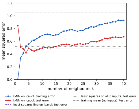
fig_1_S1. Download: PDF · SVGSee also (companion courses): Bayesian and Probabilistic Machine Learning, Section 1.1 (training and test error of polynomial fits) and the curve-fitting demo; Foundations of Deep Learning, Section 1.2.4 (model complexity).
1.2 Example 1: Email Spam
pp. 2–3 The data are 4601 email messages, each labelled genuine email or spam (junk email): 2788 email and 1813 spam (39.4%). For each message the inputs are the relative frequencies of 48 words and 6 characters (the percentage of the message's words that equal the word, or of its characters that equal the character) and 3 statistics of runs of consecutive capital letters. The goal is an automatic filter that predicts the class of a new message: a two-class classification problem. The book's website also provides a split into 3065 training and 1536 test messages, used in Chapters 9, 10 and 15.
george | you | your | hp | free | hpl | ! | our | re | edu | remove | |
|---|---|---|---|---|---|---|---|---|---|---|---|
| spam | 0.00 | 2.26 | 1.38 | 0.02 | 0.52 | 0.01 | 0.51 | 0.51 | 0.13 | 0.01 | 0.28 |
| 1.27 | 1.27 | 0.44 | 0.90 | 0.07 | 0.43 | 0.11 | 0.18 | 0.42 | 0.29 | 0.01 | |
| difference | −1.26 | 0.99 | 0.94 | −0.88 | 0.45 | −0.42 | 0.40 | 0.33 | −0.29 | −0.27 | 0.27 |
| \(t\) statistic | −15.7 | 19.9 | 27.1 | −22.3 | 16.8 | −20.1 | 17.3 | 16.4 | −11.6 | −12.4 | 19.6 |
The last two rows are not in the book: the difference of the means, and the two-sample \(t\) statistic of Filling the gap 1.3. Code: table_1_1 and class_mean_table in ch01_introduction.py.
The words make sense once one knows where the data came from: the genuine email was the work and personal mail of one person (George, at Hewlett-Packard Labs, hence george, hp, hpl), so a filter trained on it is a personalised filter.
Filling the gap 1.3: what “the largest difference” means, and why the ranking depends on the scale p. 2, Table 1.1
The caption of Table 1.1 says the words were chosen because they show the largest difference between spam and email. Which difference, among which features?
Derivation
For feature \(j\) and class \(c\in\{\text{spam},\text{email}\}\) with \(N_c\) messages, let \(\bar x_j^{(c)}=N_c^{-1}\sum_{i:g_i=c}x_{ij}\) be the class mean. Ranking the 54 word and character frequencies by \(|\bar x_j^{(\rm spam)}-\bar x_j^{(\rm email)}|\) reproduces Table 1.1 exactly: the same eleven features, in the order of the book's columns. The three capital-run features must be left out: they are lengths, not percentages, and their mean differences (about 7, 86 and 309) would dominate any list.
Even among percentages the ranking is scale-dependent: a common word such as you can differ by a whole percentage point, while a rare but telling word such as remove (0.28% against 0.01%) cannot. A scale-free alternative divides each difference by its standard error,
with \(s_j^{2(c)}\) the sample variance within class \(c\) (the unequal-variance, or Welch, two-sample statistic). By \(|t_j|\) the top eleven become your, hp, hpl, you, 000, remove, $, !, free, our, george: george falls from first to eleventh, because its large mean difference comes with a very large spread among genuine emails (most of them never mention George), while 000 and $ enter. Neither ranking measures how useful a feature is for classification, which depends on the whole distribution and on the other features; the book returns to the importance of spam features in Sections 10.13.1 and 15.3.2, and to ranking many features by \(t\) statistics in Section 18.7. ∎
The book then sketches two hand-made rules, to show what a learning method must decide (which features, and how to combine them):
\[ \text{spam if } (\%\text{george}<0.6)\ \&\ (\%\text{you}>1.5),\quad\text{otherwise email}; \] \[ \text{spam if } 0.2\cdot\%\text{you}-0.3\cdot\%\text{george}>0,\quad\text{otherwise email}. \]Result 1.5 (the book's two rules as classifiers) p. 2
(a) The first rule classifies as spam the inputs in the region \(\{x:x_{\rm george}<0.6,\ x_{\rm you}>1.5\}\), an intersection of two half-spaces bounded by planes perpendicular to coordinate axes: the region a classification tree with two splits produces (Chapter 9).
(b) The second rule is a linear classifier, \(\hat G(x)=\text{spam}\) iff \(w^\T x>0\), with \(w\) having \(0.2\) in the you coordinate, \(-0.3\) in the george coordinate and 0 elsewhere: the half-space \(x_{\rm you}>1.5\,x_{\rm george}\) bounded by a hyperplane through the origin (Chapter 4). Since frequencies are nonnegative, every message that does not contain “george” is classified as spam as soon as it contains “you”.
(c) On the 4601 messages the first rule misclassifies 28.7% (28.0% of the training set, 30.1% of the test set), flagging 726 of the 2788 genuine emails; the second misclassifies 35.1% (34.8%, 35.9%), flagging 1411 genuine emails (more than half). Calling every message email misclassifies 39.4%.
Proof
(a) and (b) restate the rules. For (b),
\[ 0.2x_{\rm you}-0.3x_{\rm george}>0\iff x_{\rm you}>1.5x_{\rm george}; \]with \(x_{\rm george}=0\) this holds iff \(x_{\rm you}>0\). (c) is a count over the data (spam_rule and confusion in the code); the trivial rule's error is the proportion of spam, \(1813/4601\). The rules were written to illustrate, not to perform: Chapter 9 fits an additive logistic regression with a test error near 5%, and Chapters 10 and 15 do better still. ∎
p. 3 The book adds that not all errors are equal: filtering out a good email is worse than letting a spam through. Decision theory says how to act on that.
Result 1.6 (unequal costs move the threshold) p. 3; Section 2.4, (2.21)
Let \(\eta(x)=\Pr(\text{spam}\given X=x)\), let flagging a genuine email cost \(c>0\) and letting a spam through cost 1, with correct decisions free. The rule of minimal risk is
\[ \hat G(x)=\text{spam}\iff\eta(x)>\frac{c}{1+c}, \]with minimal risk \(\E\min\{c\,(1-\eta(X)),\ \eta(X)\}\). For \(c=1\) this is the Bayes classifier (threshold \(\tfrac12\)); for \(c=10\) a message is flagged only when it is spam with probability above \(10/11\approx0.909\).
Proof
This is (2.21) with \(K=2\) and loss matrix \(L(\text{email},\text{spam})=c\), \(L(\text{spam},\text{email})=1\). At \(x\), flagging costs \(c\,(1-\eta(x))\) on average and keeping costs \(\eta(x)\). Flag iff \(c(1-\eta)<\eta\iff\eta>c/(1+c)\). By Filling the gap 1.1 the pointwise choice minimises the risk, whose value is the expectation of the smaller of the two conditional costs. ∎
In practice \(\eta\) is unknown, and a rule from a restricted family (boxes, half-planes) is chosen to minimise the cost-weighted training error
\[ \frac1N\sum_i\{c\,\ind(g_i=\text{email},\hat G(x_i)=\text{spam})+\ind(g_i=\text{spam},\hat G(x_i)=\text{email})\}. \]For boxes on the pair (george, remove) with \(c=10\), the best thresholds on the training set flag every message that contains “remove” and not “george”: only 17 of 1847 genuine training emails (10 of 941 in the test set) are flagged, at the price of letting 58% of the spam through.
See also (companion course): Bayesian and Probabilistic Machine Learning, Section 1.5.2 (minimising the expected loss) and its decision theory demo.
Where the spam data return. Additive logistic regression (Section 9.1.2), classification trees (9.2.5), the patient rule induction method (9.3.1), MARS (9.4.1), boosting (10.8, with variable importance in 10.13.1), random forests (Chapter 15) and ensemble learning (16.3.1).
1.3 Example 2: Prostate Cancer
pp. 3–4 The data come from a study by Stamey et al. (1989) of 97 men about to undergo radical prostatectomy. The response is the logarithm of prostate-specific antigen, lpsa; the eight inputs are log cancer volume (lcavol), log prostate weight (lweight), age, log of the amount of benign prostatic hyperplasia (lbph), seminal vesicle invasion (svi, 0 or 1), log of capsular penetration (lcp), Gleason score (gleason) and the percentage of Gleason scores 4 or 5 (pgg45). The output is quantitative, so this is a regression problem.
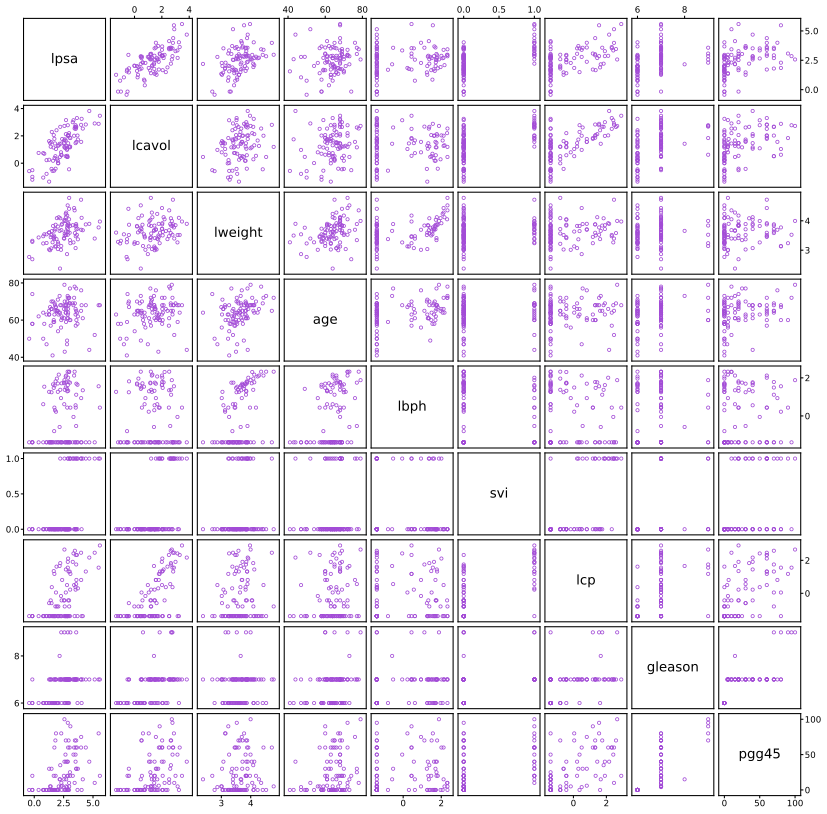
fig_1_1. Reproduces Hastie, Tibshirani and Friedman (2009), Figure 1.1. Download: PDF · SVGThe book's verdict is that some correlations are evident but a good predictive model is hard to build by eye. Two features of the picture matter later. First, several inputs are strongly correlated with each other (lcavol with lcp, svi with lcp), which is why the coefficients of a multiple regression are not the same as the one-input slopes (Chapter 3). Second, the floors in lbph and lcp mean that a straight line in those inputs cannot be the whole story.
Filling the gap 1.4: the corrected observation in the book's footnote p. 3, footnote 1
The footnote says that subject 32 had lweight 6.1 in the first edition, a 449 g prostate, and that the correct weight is 44.9 g.
Check
The variable is the natural logarithm of the weight in grams. The corrected value is \(\ln44.9=3.8044\), and the data file on the book's website has exactly 3.804438 for subject 32, so the data used here and in later chapters are the corrected ones. The first-edition value 6.1 corresponds to \(e^{6.1}\approx446\) g; the footnote's 449 g is \(e^{6.107}\), so the printed 6.1 was a rounded 6.107. Either way the error was a factor of ten in the weight (a misplaced decimal point), which on the log scale is an outlier of \(\ln10=2.30\) in a variable whose standard deviation is about 0.43: a reminder to look at scatterplots, where such a point stands out, before fitting anything. ∎
Result 1.7 (least squares with one input)
For data \((x_i,y_i)\), \(i=1,\dots,N\), with \(x\) not constant, the least-squares line \(\hat y=\hat\beta_0+\hat\beta_1x\) has
\[ \hat\beta_1=\frac{\sum_i(x_i-\bar x)(y_i-\bar y)}{\sum_i(x_i-\bar x)^2}=r_{xy}\frac{s_y}{s_x},\qquad \hat\beta_0=\bar y-\hat\beta_1\bar x, \]and its training error is \((1-r_{xy}^2)\) times that of the mean, \(\frac1N\sum_i(y_i-\bar y)^2\). If \(x\in\{0,1\}\), the fitted values are the two group means: \(\hat\beta_0=\bar y_{(0)}\) and \(\hat\beta_1=\bar y_{(1)}-\bar y_{(0)}\).
Proof
Setting the derivatives of \(\sum_i(y_i-\beta_0-\beta_1x_i)^2\) to zero gives \(\sum_ie_i=0\) and \(\sum_ix_ie_i=0\) for the residuals \(e_i=y_i-\beta_0-\beta_1x_i\). The first gives \(\beta_0=\bar y-\beta_1\bar x\); substituting, the second becomes \(\sum_i(x_i-\bar x)\{(y_i-\bar y)-\beta_1(x_i-\bar x)\}=0\), whose solution is \(\hat\beta_1\); dividing numerator and denominator by \(N\) gives \(r_{xy}s_y/s_x\). The residual sum of squares is
\[ \sum(y_i-\bar y)^2-\hat\beta_1^2\sum(x_i-\bar x)^2=(1-r_{xy}^2)\sum(y_i-\bar y)^2. \]For a 0/1 input, the conditions \(\sum_ie_i=0\) and \(\sum_ix_ie_i=0\) say that the residuals sum to zero within the group \(x=1\) and hence also within the group \(x=0\), so the fitted value in each group, \(\hat\beta_0\) and \(\hat\beta_0+\hat\beta_1\), is that group's mean. ∎
On the 67 training men, the line on lcavol is \(\widehat{\text{lpsa}}=1.516+0.713\,\text{lcavol}\), with training error 0.665 and test error 0.480; the line on svi joins the means 2.094 (52 men without seminal vesicle invasion) and 3.695 (15 men with). The full multiple regression, its standardised coefficients and the selection and shrinkage methods built on it are the subject of Chapter 3.
Where the prostate data return. Throughout Chapter 3: the least-squares fit (Section 3.2.1), best-subset and stepwise selection (3.3), ridge regression and the lasso (3.4), least angle regression (3.4.4), principal components and partial least squares (3.5), incremental forward stagewise regression (3.8.1); and again for penalised regression in Section 16.2.1.
1.4 Example 3: Handwritten Digit Recognition
pp. 4–5 The data are digits cut from handwritten ZIP codes on US postal envelopes, one digit per image, normalised to roughly the same size and orientation. Each image is a \(16\times16\) grid of grey levels, so the input is a vector in \(\R^{256}\) and the output is one of the ten classes \(0,\dots,9\). The book's website provides 7291 training and 2007 test images.
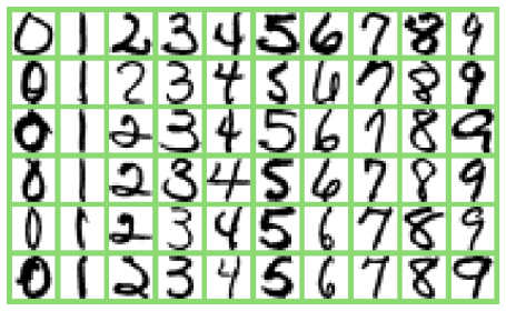
fig_1_2. Reproduces Hastie, Tibshirani and Friedman (2009), Figure 1.2. Download: PDF · SVGFilling the gap 1.5: an image as a vector, and the scale of the grey levels p. 4
The book describes the images as 8-bit grey levels from 0 to 255; the files on its website hold values between \(-1\) and \(1\). Does the scale matter?
Derivation
An image with pixels \(v_{rc}\), \(r,c=1,\dots,16\), becomes the input vector \(x\in\R^{256}\) by stacking its rows, \(x_{16(r-1)+c}=v_{rc}\). Every method in the book sees only this vector, so it knows nothing of which pixels are neighbours; Section 11.7 (networks with local, shared weights on these data) and Section 13.3.3 (tangent distance) build that knowledge back in.
The rescaling \(v\mapsto\alpha v+\beta\) with \(\alpha=2/255\), \(\beta=-1\) applies the same affine map to every coordinate. Then
\[ \|(\alpha x+\beta\mathbf 1)-(\alpha x'+\beta\mathbf 1)\|=\alpha\|x-x'\|: \]all Euclidean distances are multiplied by the same \(\alpha>0\), so the ordering of distances, and hence any nearest-neighbour classifier, is unchanged. The same holds for least squares with an intercept (the fitted values are unchanged by an affine change of all inputs), but not for methods with a penalty on the coefficients, such as ridge regression, where the size of the inputs sets the effective amount of shrinkage (Chapter 3). ∎
p. 5 The task demands a very low error rate, since a misread digit sends mail astray. The book notes that some images can be put in a “don't know” category and sorted by hand. Decision theory says exactly when.
Result 1.8 (the reject option) p. 5
Let \(p_k(x)=\Pr(G=k\given X=x)\), \(k=1,\dots,K\). Suppose a correct classification costs 0, a wrong one costs 1, and “don't know” costs \(d\) with \(0<d<1\). The rule of minimal risk classifies to \(\argmax_kp_k(x)\) when \(\max_kp_k(x)\ge1-d\), and rejects when \(\max_kp_k(x)<1-d\). If \(d\ge1-1/K\) it never rejects (for ten digits, a reject costing \(0.9\) or more is never worth it).
Proof
At \(x\), classifying to \(k\) costs \(1-p_k(x)\) on average, smallest for the most probable class, at \(1-\max_kp_k(x)\); rejecting costs \(d\). Reject iff \(d<1-\max_kp_k(x)\); by Filling the gap 1.1 this pointwise rule minimises the risk. Since the \(K\) probabilities sum to 1, \(\max_kp_k(x)\ge1/K\), so \(1-\max_kp_k\le1-1/K\le d\) and rejection never pays when \(d\ge1-1/K\). This is Chow's (1970) rule; a version with a general loss matrix is in the companion course, Result 1.17. ∎
See also (companion course): Bayesian and Probabilistic Machine Learning, Section 1.5.3, the reject option.
Where the digits return. Neural networks, including networks with constrained, convolution-like weights (Section 11.7); nearest-neighbour classifiers and the tangent distance that makes them invariant to small rotations and shifts (13.3, 13.3.3); principal components of the handwritten threes (14.5.1) and kernel principal components (14.5.4).
1.5 Example 4: DNA Expression Microarrays
pp. 5–6 A DNA microarray measures, for each of thousands of genes at once, the amount of messenger RNA in a sample of cells relative to a reference sample. The target and reference are labelled with red and green dyes and hybridised to the DNA printed on a glass slide; the recorded value for each gene is the log ratio of red to green intensity, typically between about \(-6\) and \(6\), positive when the gene is more expressed in the target. Collecting the experiments as columns gives a matrix with one row per gene. Here: 6830 genes and 64 samples, cancer cell lines from different tumours (the NCI60 panel; Ross et al., 2000).
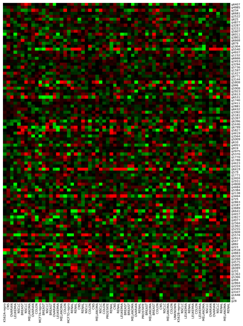
fig_1_3. Reproduces Hastie, Tibshirani and Friedman (2009), Figure 1.3. Download: PDF · SVGThe book lists the questions one asks of such data: (a) which samples are most alike across genes; (b) which genes are most alike across samples; (c) which genes are unusually high or low in particular samples. It suggests viewing these as unsupervised problems: for (a), the 64 samples are points in \(\R^{6830}\) to be clustered.
Result 1.9 (distance between standardised profiles is a correlation) p. 5; Section 14.3.3, (14.22)
For \(u,v\in\R^p\), let \(\bar u=\frac1p\sum_ju_j\), \(s_u^2=\frac1p\sum_j(u_j-\bar u)^2>0\), \(z_u=(u-\bar u\mathbf 1)/s_u\), similarly for \(v\), and let \(r_{uv}\) be the correlation (14.22) between the two profiles (computed across the \(p\) coordinates). Then
\[ \|z_u-z_v\|^2=2p\,(1-r_{uv}). \]So after standardising each sample, clustering by squared Euclidean distance is the same as clustering by correlation: two samples are close when their expression profiles rise and fall together across genes, whatever their overall level and spread.
Proof
By construction \(\sum_jz_{u,j}=0\) and \(\|z_u\|^2=\sum_j(u_j-\bar u)^2/s_u^2=p\), likewise \(\|z_v\|^2=p\), and
\[ z_u^\T z_v=\sum_j(u_j-\bar u)(v_j-\bar v)/(s_us_v)=p\,r_{uv} \]by the definition of the correlation. Hence
\[ \|z_u-z_v\|^2=\|z_u\|^2+\|z_v\|^2-2z_u^\T z_v=2p-2p\,r_{uv}. \]∎
For the NCI60 data with \(p=6830\), the identity holds to rounding error, and the nearest neighbour of a sample in this distance has the same tumour label for 40 of the 64 samples: question (a) has a partly predictable answer, which Section 14.3.8 pursues with k-means and Section 14.3.12 with hierarchical clustering.
The book also remarks that the matrix could be treated as a regression with two categorical predictors, gene and sample, and the expression level as response, but that this is probably less useful. The next result shows why, on these data.
Result 1.10 (the additive gene-plus-sample model) p. 5
Let \(x_{gs}\), \(g=1,\dots,n\) (genes), \(s=1,\dots,m\) (samples), be a complete matrix, and fit \(x_{gs}\approx\mu+\alpha_g+\beta_s\) with \(\sum_g\alpha_g=\sum_s\beta_s=0\) by least squares. With dots for averages, the solution is
\[ \hat\mu=\bar x_{\cdot\cdot},\qquad\hat\alpha_g=\bar x_{g\cdot}-\bar x_{\cdot\cdot},\qquad\hat\beta_s=\bar x_{\cdot s}-\bar x_{\cdot\cdot}, \]and, with residuals \(\hat r_{gs}=x_{gs}-\bar x_{g\cdot}-\bar x_{\cdot s}+\bar x_{\cdot\cdot}\), the total sum of squares splits as
\[ \sum_{g,s}(x_{gs}-\bar x_{\cdot\cdot})^2=m\sum_g\hat\alpha_g^2+n\sum_s\hat\beta_s^2+\sum_{g,s}\hat r_{gs}^2 . \]On the NCI60 data the gene effects account for 2.95% of the total, the sample effects for 0.44%, and the residual (gene-by-sample interaction) for 96.6%.
Proof
Write \(x_{gs}-\bar x_{\cdot\cdot}=\hat\alpha_g+\hat\beta_s+\hat r_{gs}\) (an identity). The residual array has zero row sums and zero column sums:
\[ \sum_s\hat r_{gs}=m\bar x_{g\cdot}-m\bar x_{g\cdot}-m\bar x_{\cdot\cdot}+m\bar x_{\cdot\cdot}=0, \]and similarly over \(g\). Hence the three arrays \((\hat\alpha_g)\), \((\hat\beta_s)\) and \((\hat r_{gs})\), viewed as vectors in \(\R^{nm}\), are mutually orthogonal: \(\sum_{g,s}\hat\alpha_g\hat\beta_s=(\sum_g\hat\alpha_g)(\sum_s\hat\beta_s)=0\), \(\sum_{g,s}\hat\alpha_g\hat r_{gs}=\sum_g\hat\alpha_g\sum_s\hat r_{gs}=0\), and likewise for \(\hat\beta\) and \(\hat r\). Squaring the identity and summing gives the decomposition. Now take any \((\mu,\alpha,\beta)\) satisfying the constraints. Then
\[ x_{gs}-\mu-\alpha_g-\beta_s=(\hat\mu-\mu)+(\hat\alpha_g-\alpha_g)+(\hat\beta_s-\beta_s)+\hat r_{gs}, \]and the same orthogonality (the differences \(\hat\alpha-\alpha\) and \(\hat\beta-\beta\) also sum to zero) gives
\[ \sum_{g,s}(x_{gs}-\mu-\alpha_g-\beta_s)^2=nm(\hat\mu-\mu)^2+m\sum_g(\hat\alpha_g-\alpha_g)^2+n\sum_s(\hat\beta_s-\beta_s)^2+\sum_{g,s}\hat r_{gs}^2, \]which is smallest, uniquely, at \((\hat\mu,\hat\alpha,\hat\beta)\). The percentages are computed by two_way_additive in the code. ∎
The additive model can only say that some genes are high everywhere and some samples are high on every gene. Question (c), which genes are high or low in which samples, is about the interaction, and on these data the interaction is almost everything: 96.6% of the variation is what the regression view would call noise. That is the precise sense in which an unsupervised description (clusters of samples and genes, low-dimensional structure) is more useful here.
Where the microarray data return. Clustering the NCI60 samples with k-means (Section 14.3.8) and hierarchical clustering (14.3.12). Chapter 18 treats microarray-type problems with \(p\gg N\) on other data sets: nearest shrunken centroids (18.2), regularised discriminant analysis (18.3), supervised principal components (18.6), and the multiple-testing problem of finding differentially expressed genes (18.7).
1.6 Who should read this book, and how it is organized
pp. 7–8 The book is meant for researchers and students in statistics, artificial intelligence, engineering, finance and other fields who have had an elementary course in statistics, including linear regression. It describes a selection of important methods rather than a catalogue, with the emphasis on concepts and on how to judge a learning method, and it reflects the authors' statistical background together with ideas from neural networks, data mining and machine learning. Its plan is to understand simple methods before complex ones. The chapters of this course follow the book's chapters; each is described below and listed on the course home page.
| Chapter | Topic | Examples of Chapter 1 used |
|---|---|---|
| 2 | Overview of supervised learning: least squares and nearest neighbours, statistical decision theory (the source of Section 1.1.3), the curse of dimensionality, model complexity | |
| 3 | Linear methods for regression: least squares, subset selection, ridge, lasso, least angle regression, principal components and partial least squares | prostate |
| 4 | Linear methods for classification: linear regression of indicators, discriminant analysis, logistic regression, separating hyperplanes | |
| 5 | Basis expansions and regularisation: splines, smoothing splines, reproducing kernels, wavelets | |
| 6 | Kernel smoothing methods: local regression, kernel density estimation, radial basis functions | |
| 7 | Model assessment and selection: bias and variance, optimism of the training error (the source of Result 1.4), AIC, BIC, cross-validation, the bootstrap | |
| 8 | Model inference and averaging: maximum likelihood, Bayesian inference, the bootstrap, the EM algorithm, MCMC, bagging | |
| 9 | Additive models, trees and related methods: generalised additive models, CART, PRIM, MARS | spam |
| 10 | Boosting and additive trees | spam |
| 11 | Neural networks | digits |
| 12 | Support vector machines and flexible discriminants | |
| 13 | Prototype methods and nearest neighbours | digits |
| 14 | Unsupervised learning: association rules, cluster analysis, principal components, self-organising maps, independent components | microarray, digits |
| 15 | Random forests | spam |
| 16 | Ensemble learning | spam, prostate |
| 17 | Undirected graphical models | |
| 18 | High-dimensional problems, \(p\gg N\) | microarray-type data |
The book recommends reading Chapters 1–4 in sequence and treating Chapter 7 as essential, since its concepts apply to every method; the rest can be read in order or sampled. Technically demanding sections are marked with a symbol and can be skipped on a first reading. Each chapter ends with computational considerations (how the cost grows with \(N\) and \(p\)) and bibliographic notes. The website listed in the book has moved; it is now hastie.su.domains/ElemStatLearn, and it holds the data sets used here. For instructors, the authors report teaching the first edition as a two-quarter course, with enough material in the second for three quarters, and stress access to good software (they used R and S-PLUS); this course uses Python for every figure.
Exercises
Chapter 1 of the book has no exercises (they start with Chapter 2). Three short practice problems on the framework of this chapter follow, with solutions.
Practice 1.1. Under absolute error loss, show that among constant predictions \(c\) the risk \(\E|Y-c|\) is minimised by a median of \(Y\), and that the minimiser need not be unique.
Solution
For \(c<c'\), \(|y-c'|-|y-c|\) equals \(c'-c\) when \(y\le c\), \(-(c'-c)\) when \(y\ge c'\), and lies between these values in between. Hence
\[ \E|Y-c'|-\E|Y-c|\le(c'-c)\{\Pr(Y\le c)-\Pr(Y\ge c')\}, \]and similarly in the other direction, so \(c\mapsto\E|Y-c|\) is convex with right derivative \(\Pr(Y\le c)-\Pr(Y>c)\). It decreases while \(\Pr(Y\le c)<\tfrac12\) and increases once \(\Pr(Y\le c)>\tfrac12\), so its minimisers are the medians, the \(c\) with \(\Pr(Y\le c)\ge\tfrac12\) and \(\Pr(Y\ge c)\ge\tfrac12\). If \(Y\) is 0 or 1 with probability \(\tfrac12\) each, every \(c\in[0,1]\) gives \(\E|Y-c|=\tfrac12\): the minimiser is not unique. Applied conditionally on \(X=x\) this gives (2.18).
Practice 1.2. In the spam problem, suppose the only input is whether the message contains “george”, and that (approximately, from the data) \(\Pr(\text{spam})=0.394\), \(\Pr(\text{contains george}\given\text{spam})=0.004\) and \(\Pr(\text{contains george}\given\text{email})=0.28\). Find the Bayes classifier and its error rate, and the rule of Result 1.6 with \(c=10\).
Solution
By Bayes' theorem,
\[ \Pr(\text{spam}\given\text{george})=\frac{0.394\cdot0.004}{0.394\cdot0.004+0.606\cdot0.28}\approx0.009, \] \[ \Pr(\text{spam}\given\text{no george})=\frac{0.394\cdot0.996}{0.394\cdot0.996+0.606\cdot0.72}\approx0.474. \]Both are below \(\tfrac12\), so the Bayes classifier calls every message email, with error \(\Pr(\text{spam})=0.394\): the word is informative (it nearly certifies email) but, alone, never makes spam the more probable class. With \(c=10\) the threshold is \(10/11\), further away still: again everything is email. A useful rule needs more inputs, which is the point of the book's combinations of words.
Practice 1.3. A k-nearest-neighbour regression on \(N=67\) points with noise variance \(\sigma^2\) has training error 0.62 at \(k=7\). Using Result 1.4(d), what in-sample error would you expect, and what is the effective number of parameters? Take \(\sigma^2=0.5\).
Solution
The effective number of parameters is \(\Tr\bS=N/k=67/7\approx9.6\), about the same as least squares on all eight inputs (9). The optimism is \(2\sigma^2/k=2\cdot0.5/7\approx0.14\), so the expected in-sample error is about \(0.62+0.14=0.76\). (The prostate test error at \(k=7\) is 0.447: the test set is a different set of inputs, and with 30 men its standard error is large, so the comparison is rough.)
Demonstrations for this chapter
Each demonstration runs in the browser on the book's own data and links back to these notes. The ▶ Demo boxes above open them already set to the case under discussion.
| Demonstration | What you can see | Sections and results |
|---|---|---|
| Prostate cancer data: simple fits, training error and test error | lpsa against any of the eight inputs, with the training mean, a least-squares line or a k-nearest-neighbour average; training and test error against \(k\); least squares on all eight inputs. Presets: 1 line on lcavol; 2 one nearest neighbour; 3 \(k=15\); 4 a 0/1 input; 5 all eight inputs. | 1.1.4, 1.3; Results 1.3, 1.4, 1.7, Filling the gap 1.2 |
| Email spam: word frequencies by class and simple rules | The class means of the 54 word and character frequencies, ranked by difference (Table 1.1) or by \(t\) statistic; two words plotted for every message with the spam region of a box or linear rule; training and test error and a cost for flagging good email; threshold tuning on the training set. Presets: 1 Table 1.1; 2 the first rule; 3 the second rule; 4 \(t\) ranking; 5 costly false alarms. | 1.2; Filling the gap 1.3, Results 1.5, 1.6 |
The Python code that produces every figure of this page, Table 1.1 and the demonstrations' data is code/ch01_introduction.py (see the code index).
References
- Hastie, T., Tibshirani, R. and Friedman, J. (2009). The Elements of Statistical Learning: Data Mining, Inference, and Prediction, 2nd edition. Springer, New York. Chapter 1, pp. 1–8. hastie.su.domains/ElemStatLearn.
- Bishop, C. M. (2006). Pattern Recognition and Machine Learning. Springer, New York.
- Bishop, C. M. and Bishop, H. (2024). Deep Learning: Foundations and Concepts. Springer, Cham.
- Chow, C. K. (1970). On optimum recognition error and reject tradeoff. IEEE Transactions on Information Theory, 16(1), 41–46.
- Mallows, C. L. (1973). Some comments on \(C_p\). Technometrics, 15(4), 661–675.
- Ross, D. T., Scherf, U., Eisen, M. B. et al. (2000). Systematic variation in gene expression patterns in human cancer cell lines. Nature Genetics, 24(3), 227–235.
- Stamey, T., Kabalin, J., McNeal, J., Johnstone, I., Freiha, F., Redwine, E. and Yang, N. (1989). Prostate specific antigen in the diagnosis and treatment of adenocarcinoma of the prostate II: radical prostatectomy treated patients. Journal of Urology, 141(5), 1076–1083.
- Welch, B. L. (1947). The generalization of “Student's” problem when several different population variances are involved. Biometrika, 34(1–2), 28–35.
The numerical statements in the text (Table 1.1 and its \(t\) ranking, the error rates of the rules, the prostate fits and their standard errors, the optimism formulas, the distance identity and the two-way decomposition of the microarray matrix) were confirmed numerically.