Ensemble Learning
An ensemble predicts by combining many simple models. This chapter reads ensemble learning as a two-stage process: first build a large dictionary of base learners (trees, rules, or the inputs themselves), then combine them by penalised regression. Seen this way, boosting with shrinkage is a slow, greedy way of tracing a lasso-like regularisation path through the space of all trees: with uncorrelated basis functions, or whenever the lasso path is monotone, forward stagewise regression and the lasso coincide exactly, and in general stagewise fitting solves a monotone version of the lasso. Why should an L1 path work so well? Because of the bet on sparsity: when only a few basis functions matter the lasso does well and ridge does not, and when many matter nothing does well. The chapter ends with the practical consequence: grow a deliberately diverse ensemble by importance sampling, then let the lasso pick and reweight a few of its trees or rules.
Ch. 1 Introduction Ch. 2 Supervised learning Ch. 3 Linear regression Ch. 4 Linear classification Ch. 5 Basis expansions Ch. 6 Kernel smoothing Ch. 7 Model assessment Ch. 8 Inference and averaging Ch. 9 Additive models and trees Ch. 10 Boosting Ch. 11 Neural networks Ch. 12 SVMs Ch. 13 Nearest neighbours Ch. 14 Unsupervised learning Ch. 15 Random forests Ch. 16 Ensembles Ch. 17 Graphical models Ch. 18 High-dimensional problems
How to read these notes
They follow the book. Sections carry the book's numbers (16.2.1, 16.3.2, ...) and every displayed equation that appears in the book carries the book's own equation number, e.g. \((16.9)\), so you can read these notes next to the book. Equations without a number are steps that the book skips.
Filling the gaps. Wherever the book says that something "can be shown", leaves it to an exercise, or states a property without proof, an orange Filling the gap box or a proof gives the full argument. Proofs and derivations start hidden: open one with its bar, or use the button below.
Figures and demonstrations. Every figure of the chapter that is computed from data or a simulation is reproduced from scratch by the Python code (the lasso and stagewise paths, the bet-on-sparsity simulation, the boosting and ISLE algorithms and the post-processing lasso are all implemented there and confirmed against standard libraries). Figure 16.9 is a drawing of a small tree and is described in words. The ▶ Demo boxes open an interactive demonstration already set to the case being discussed.
Main reference
T. Hastie, R. Tibshirani and J. Friedman, The Elements of Statistical Learning: Data Mining, Inference, and Prediction, 2nd edition, Springer (2009), Chapter 16, pages 605–624 (book website, with the data sets: hastie.su.domains/ElemStatLearn). Section, equation, figure and exercise numbers below refer to this book. Further reading is listed in the references.
The explanations, derivations, figures and code are my own; equations are cited by their numbers in the book.
Companion courses
Parts of this chapter also appear in the two companion courses on this site. The overlapping material is:
- Section 16.1 (ensembles, committees, Bayesian averaging as an ensemble): Bayesian and Probabilistic Machine Learning, Section 14.1 (Bayesian model averaging, Result 14.1) and Section 14.2 (committees, Result 14.2); Foundations of Deep Learning, Section 9.6 (model averaging, Result 9.11).
- Section 16.2 (boosting as stagewise fitting): Section 14.3 of the companion course and Result 14.4; with squared error each stage fits the residuals: Filling the gap 14.10.
- Sections 16.2.1–16.2.2 (why an L1 penalty produces exact zeros, L1 against L2): Foundations of Deep Learning, Section 9.2.2, Result 9.6 and Filling the gap 9.5, with the L1 versus L2 paths demo.
- Section 16.2.3 (early stopping picks a point on a regularisation path): Foundations of Deep Learning, Section 9.3.1 and Result 9.7 (early stopping as weight decay).
Where a proof there is the same, these notes state the result, sketch the argument and link to it. New here: forward stagewise against the lasso (exact agreement for orthogonal dictionaries and monotone paths, stagewise as steepest descent in the L1 geometry), the risk calculation behind the bet on sparsity, the monotone lasso and its optimal direction, the L1 margin as an L∞ distance and the margin-maximising limit, importance-sampled ensembles and the half-sample/bootstrap equivalence, lasso post-processing and rule ensembles.
The chapter at a glance
- 16.1 An ensemble is a dictionary plus a way of combining it; error-correcting output codes combine many two-class problems, and a code with minimum Hamming distance \(d\) corrects \(\lfloor (d-1)/2\rfloor\) wrong votes (Filling the gap 16.1).
- 16.2.1 Boosting with shrinkage behaves like the lasso over the dictionary of all trees. Forward stagewise (Algorithm 16.1) is steepest descent in the L1 geometry (Result 16.2); it reproduces the lasso exactly for orthogonal dictionaries (Result 16.3) and whenever the lasso path is monotone (Result 16.4). The lasso does not shrink every coefficient below its least-squares value (note), but it does shrink the L1 norm (Result 16.1).
- 16.2.2 In a sparse problem the lasso's risk is of the order of the number of nonzero coefficients times \(\log p\), while ridge's is of order \(p\) (Result 16.5); in a dense problem nothing can do well. Figure 16.2 is reproduced, with a correction to the definition of its noise-to-signal ratio for classification (note).
- 16.2.3 Under strong correlation the lasso path swings while FS0 stays monotone; FS0 is the lasso path that is monotone in the doubled dictionary and its direction is optimal per unit of arc length (Results 16.6–16.7, Exercise 16.2). The L1 margin is an L∞ distance (Result 16.8), and L1-constrained exponential-loss fits tend to the margin-maximising solution (Result 16.9).
- 16.3 Importance-sampled learning ensembles (Algorithm 16.2) contain bagging, random forests and (stochastic) gradient boosting as special cases; a lasso post-processor (16.9) keeps a fraction of the trees at the same or lower test error (Figures 16.6–16.8). Rules extracted from trees span the trees (Result 16.10, Exercise 16.3) and give the rule ensembles of Figure 16.10.
Notation. Training data \((x_i,y_i)\), \(i=1,\dots,N\), \(x_i\in\R^p\). A dictionary \(\cT=\{T_k\}_{k=1}^K\) of basis functions (typically trees); \(\bT\) is the \(N\times K\) matrix with entries \(T_k(x_i)\). Coefficients \(\ba=(\alpha_k)\); \(|\ba|_1=\sum_k|\alpha_k|\). The residual is \(\br=\by-\bT\ba\) and the "correlations" are the inner products \(c_k=\langle T_k,\br\rangle=\sum_iT_k(x_i)r_i\). For the linear-model examples the dictionary is the set of (centred, scaled) inputs.
Prerequisites. The lasso, least angle regression and incremental forward stagewise regression (Sections 3.4.2, 3.4.4 and 3.8.1), bagging and stacking (Sections 8.7 and 8.8), boosting (Sections 10.10 and 10.12), and the support vector machine as a penalised method (Section 12.3.2). Random forests are the book's Chapter 15.
16.1 Introduction
pp. 605–606 An ensemble builds a prediction model by combining a collection of simpler base models. Several are already familiar: bagging (Section 8.7) and random forests average trees fitted to perturbed data; boosting (Chapter 10) adds trees one at a time, each one depending on the earlier ones, and weights their votes; stacking (Section 8.8) learns how to weight models of different kinds. Any dictionary method, for instance regression splines, can be read the same way, with the basis functions as the "weak learners"; and Bayesian nonparametric regression averages many candidate models with posterior weights.
The book splits ensemble learning into two tasks: (i) build a population of base learners from the training data, and (ii) combine them into one predictor. The rest of the chapter studies boosting, which does both at once by a regularised, supervised search through a huge space of weak learners, and then separates the two stages again (Section 16.3).
See also (companion courses): committees and why averaging helps (Result 14.2), Bayesian model averaging, and Result 9.11 (committee error, correlations and the ambiguity decomposition).
Error-correcting output codes. An early ensemble for \(K\)-class problems (Dietterich and Bakiri, 1995): a \(K\times L\) binary coding matrix \(\mathbf C\) gives each class a codeword (a row) and each column \(\ell\) defines a two-class problem that merges the classes into two groups. The book's Table 16.1 shows a few rows and columns of a 15-bit code for the ten digits; it is not reproduced here because the full matrix is not printed. The method:
- train a separate two-class classifier for each of the \(L\) columns;
- at a test point \(x\), let \(\hat p_\ell(x)\) be the predicted probability of a 1 in column \(\ell\);
- score each class by \(\delta_k(x)=\sum_{\ell=1}^L|C_{k\ell}-\hat p_\ell(x)|\) and predict the class with the smallest \(\delta_k\).
The codewords carry more bits than needed (\(\lceil\log_2 10\rceil=4\) bits would distinguish ten classes), and the redundant bits let the decoder absorb some wrong column classifiers. The book's full 15-bit code has minimum Hamming distance 7 between rows. James and Hastie (1998) found random codes as good as carefully designed ones, and argued that the gain comes mainly from variance reduction, as in bagging: different columns give different trees, and the decoding step averages them.
Filling the gap 16.1: what "error correcting" means, and how the decoding generalises it p. 606
If the minimum Hamming distance between codewords is \(d\), then decoding to the nearest codeword recovers the true class whenever at most \(\lfloor(d-1)/2\rfloor\) of the \(L\) column classifiers are wrong; with \(d=7\), any three wrong columns are tolerated. The score \(\delta_k\) is exactly the Hamming distance when the \(\hat p_\ell\) are 0 or 1, and in general an L1 distance from the vector of probabilities to the codeword.
Derivation
Let \(c_k\in\{0,1\}^L\) be the codewords, \(d_H\) the Hamming distance (number of differing entries), which is a metric. Suppose the true class is \(k\) and the vector of hard predictions \(\hat c\in\{0,1\}^L\) differs from \(c_k\) in \(e\le\lfloor(d-1)/2\rfloor\) places, so \(2e\le d-1\lt d\). For any other class \(j\), the triangle inequality gives \[d_H(\hat c,c_j)\ge d_H(c_k,c_j)-d_H(\hat c,c_k)\ge d-e>e=d_H(\hat c,c_k)\]. So \(c_k\) is the unique nearest codeword. With \(d=7\), \(e\le3\).
For \(\hat p_\ell\in\{0,1\}\), \(|C_{k\ell}-\hat p_\ell|\) is 1 exactly when the bits differ, so \(\delta_k=d_H(\hat c,c_k)\). For probabilities in \([0,1]\), \(\delta_k=\|c_k-\hat{\mathbf p}\|_1\), and a confident wrong column costs nearly a full bit while an uncertain one (\(\hat p_\ell\approx\frac12\)) costs about half a bit for every class, so it barely affects the ranking. The one-hot "indicator" code of Section 4.2 has \(d=2\): it detects a single error but cannot correct any. ∎
16.2 Boosting and Regularization Paths
p. 607 The first edition of the book suggested an analogy between the sequence of models produced by gradient boosting and regularised fitting in a very high-dimensional feature space. This section develops it, starting from the observation that a boosted version of linear regression is close to the lasso.
16.2.1 Penalized Regression
pp. 607–610 Take as basis functions every regression tree with \(J\) terminal nodes that can be realised on the training data, \(\cT=\{T_k\}\), and consider the linear model
\[ f(x)=\sum_{k=1}^K\alpha_kT_k(x), \tag{16.1} \]with \(K=\mathrm{card}(\cT)\), far larger than any training set. Least squares is hopeless, so penalise: let \(\hat\ba(\lambda)\) solve
\[ \min_{\ba}\Big\{\sum_{i=1}^N\Big(y_i-\sum_{k=1}^K\alpha_kT_k(x_i)\Big)^2+\lambda\cdot J(\ba)\Big\}, \tag{16.2} \]with, for example,
\[ J(\ba)=\sum_{k=1}^K|\alpha_k|^2\quad\text{(ridge regression)}, \tag{16.3} \] \[ J(\ba)=\sum_{k=1}^K|\alpha_k|\quad\text{(lasso)}. \tag{16.4} \]The book's display also carries the number (16.5) on an empty line; no equation (16.5) exists. With moderate to large \(\lambda\) the lasso solution is sparse: only a few trees enter (16.1). Which ones depends on the target, so sparsity is the right prior in the sense of the next section.
See also: Section 3.4.2 (the lasso) and, in the companion course, Filling the gap 9.5 (why the L1 penalty gives exact zeros and no \(q>1\) does).
Result 16.1 (the penalty of the solution falls as \(\lambda\) grows; the fit gets worse)
Let \(R(\ba)\) be any loss and \(J\ge0\) any penalty, and let \(\hat\ba(\lambda)\) minimise \(R(\ba)+\lambda J(\ba)\). If \(0\le\lambda_1\lt\lambda_2\), then \(J(\hat\ba(\lambda_2))\le J(\hat\ba(\lambda_1))\) and \(R(\hat\ba(\lambda_2))\ge R(\hat\ba(\lambda_1))\). For the lasso: \(|\hat\ba(\lambda)|_1\) never increases with \(\lambda\), and is at most the L1 norm of any least-squares solution.
Proof
Write \(\ba_1=\hat\ba(\lambda_1)\), \(\ba_2=\hat\ba(\lambda_2)\). Optimality of each at its own \(\lambda\): \[R(\ba_1)+\lambda_1J(\ba_1)\le R(\ba_2)+\lambda_1J(\ba_2)\] and \[R(\ba_2)+\lambda_2J(\ba_2)\le R(\ba_1)+\lambda_2J(\ba_1)\]. Adding the two and cancelling \(R(\ba_1)+R(\ba_2)\): \((\lambda_2-\lambda_1)\big(J(\ba_2)-J(\ba_1)\big)\le0\), so \(J(\ba_2)\le J(\ba_1)\). Putting this back in the first inequality, \[R(\ba_1)-R(\ba_2)\le\lambda_1(J(\ba_2)-J(\ba_1))\le0\]. Letting \(\lambda_1=0\) (a least-squares solution, any one) gives the last claim. ∎
Note on the book: the lasso shrinks the norm, not necessarily every coefficient
The book says that the coefficients the lasso does not set to zero have absolute values smaller than their least-squares values, \(|\hat\alpha_k(\lambda)|\lt|\hat\alpha_k(0)|\). That is true for an orthonormal dictionary, where \(\hat\alpha_k(\lambda)=\sgn(z_k)(|z_k|-\lambda)_+\) is the soft-thresholded least-squares coefficient \(z_k\), and it holds on the prostate data, but it is false in general: only the L1 norm is guaranteed to shrink (Result 16.1). A three-input example (inputs with unit variances and correlations \(\rho_{12}=0.7\), \(\rho_{13}=-0.3\), \(\rho_{23}=0.2\), population least-squares coefficients \((1,\,0.4,\,-0.4)\), no noise) has lasso path knots \((0,0,0)\), \((1.114,0,0)\), \((1.171,0,-0.057)\), \((1,0.4,-0.4)\): the first coefficient overshoots its least-squares value by 17% before the other inputs pull it back (computed exactly with least angle regression). Footnote 2 of the book also needs a qualification: when \(K>N\) the minimum-L1-norm interpolating solution need not be unique (two identical trees on the training data can share their weight in any proportion, as in Exercise 3.28); it is unique when the columns are in general position.
Algorithm 16.1 (forward stagewise linear regression) p. 608
- Initialise \(\check\alpha_k=0\), \(k=1,\dots,K\). Set \(\varepsilon>0\) to a small constant and \(M\) large.
- For \(m=1\) to \(M\):
- \[(\beta^*,k^*)=\argmin_{\beta,k}\sum_{i=1}^N\big(y_i-\sum_{l=1}^K\check\alpha_lT_l(x_i)-\beta T_k(x_i)\big)^2\];
- \[\check\alpha_{k^*}\leftarrow\check\alpha_{k^*}+\varepsilon\cdot\sgn(\beta^*)\].
- Output \(f_M(x)=\sum_{k=1}^K\check\alpha_kT_k(x)\).
All coefficients start at zero (\(\lambda=\infty\) in (16.2)). Each step picks the basis function that best fits the current residuals and moves its coefficient by a tiny amount \(\varepsilon\) towards that fit; all other coefficients stay where they are. After \(M\lt\infty\) steps many coefficients are still zero and the others are typically smaller in absolute value than at least squares, so the result resembles the lasso with \(M\) playing the role of \(1/\lambda\). If run long enough with \(K\lt N\), it stops changing when all residual correlations vanish, i.e. at a least-squares fit (\(\lambda=0\)).
Result 16.2 (what step 2(a) picks, and forward stagewise as steepest descent in the L1 geometry)
(a) Step 2(a) chooses the basis function maximising \(|c_k|/\|T_k\|\), with \(c_k=\langle T_k,\br\rangle\), and \(\sgn\beta^*=\sgn c_{k^*}\); when all basis functions have the same norm it is the one most correlated with the residual. All \(\beta^*=0\) only when \(\bT^\T\br=\mathbf 0\), the least-squares normal equations.
(b) Let \(R(\ba)=\frac12\|\by-\bT\ba\|^2\), with \(\nabla R=-\bT^\T\br=-\bc\). Among all moves \(\boldsymbol\delta\) of L1 length \(\varepsilon\), the first-order decrease \(-\nabla R^\T\boldsymbol\delta=\bc^\T\boldsymbol\delta\) is largest for \(\boldsymbol\delta=\varepsilon\,\sgn(c_{k})\,e_{k}\) with \(k\) maximising \(|c_k|\): the step of Algorithm 16.1 for equal-norm basis functions. After \(M\) steps the path has L1 arc length exactly \(M\varepsilon\).
Proof
(a) For a fixed \(k\), the criterion is \(\|\br-\beta T_k\|^2\) (writing \(T_k\) for the vector \((T_k(x_i))_i\)), minimised at \(\beta=c_k/\|T_k\|^2\) with minimum \(\|\br\|^2-c_k^2/\|T_k\|^2\) (Result 10.1 of Chapter 10). Minimising over \(k\) maximises \(c_k^2/\|T_k\|^2\), and the sign of \(\beta^*\) is that of \(c_{k^*}\). If every \(c_k=0\) then \(\bT^\T(\by-\bT\check\ba)=\mathbf 0\).
(b) By Hölder's inequality \[\bc^\T\boldsymbol\delta\le\|\bc\|_\infty\|\boldsymbol\delta\|_1=\varepsilon\max_k|c_k|\], with equality for the stated \(\boldsymbol\delta\). Each step changes one coordinate by \(\varepsilon\), so the arc length \(\sum_m\|\ba^{(m)}-\ba^{(m-1)}\|_1=M\varepsilon\). (With the Euclidean norm instead, the steepest move would be along \(\bc\) itself, changing every coefficient at once: gradient descent, which traces a ridge-like path; see Result 9.7 of the companion course.) ∎
The book's Figure 16.1 compares the two procedures on the prostate data of Chapter 3, with the eight inputs themselves as the dictionary.
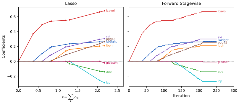
fig_16_1. Reproduces Hastie, Tibshirani and Friedman (2009), Figure 16.1. Download: PDF · SVGThe resemblance is more than qualitative in two situations.
Result 16.3 (uncorrelated basis functions: stagewise is the lasso) p. 609
Suppose the basis functions are orthonormal on the training data, \(\bT^\T\bT=\bI\), and let \(z_k=\langle T_k,\by\rangle\) be the least-squares coefficients. Run Algorithm 16.1 for \(M\) steps with \(M\varepsilon=t\lt\sum_k|z_k|\). Then every coefficient is within \(\varepsilon\) of the lasso solution at the level \(L_M=\max_k|c_k|\), \(\sgn(z_k)(|z_k|-L_M)_+\), whose L1 norm is within \(K\varepsilon\) of \(t\). Hence as \(\varepsilon\downarrow0\), \(M\uparrow\infty\), \(M\varepsilon\to t\), Algorithm 16.1 converges to the lasso solution with bound \(t\), uniformly along the path.
Proof
With \(\bT^\T\bT=\bI\), \(c_k=\langle T_k,\by-\bT\ba\rangle=z_k-\alpha_k\), and the lasso solution of (16.2) with penalty \(2\lambda'\) (so that the threshold is \(\lambda'\)) is coordinate-wise soft thresholding, \(\hat\alpha_k=\sgn(z_k)(|z_k|-\lambda')_+\) (Section 3.4.3).
Let \(L_m=\max_k|c_k|\) after \(m\) steps. A step lowers the chosen \(|c_k|\) by \(\varepsilon\) (as long as \(L_m\ge\varepsilon\), it does not overshoot zero) and leaves the others unchanged, so \(L_m\) is nonincreasing. Claim: every coordinate that has been moved satisfies \(L_m-\varepsilon\le|c_k|\le L_m\) with \(\sgn c_k=\sgn z_k\), and has never been moved backwards. Induction: when \(k\) is moved, \(|c_k|\) was the maximum \(L_{\text{old}}\) and becomes \(L_{\text{old}}-\varepsilon\ge L_m-\varepsilon\) for every later \(m\) (because \(L\) only decreases); it stays \(\le L_m\) by the definition of the maximum; as \(|c_k|\ge L_m-\varepsilon\ge0\) its sign never flips, so each later move of \(k\) is again towards \(z_k\). Unmoved coordinates have \(\alpha_k=0\) and \(|z_k|=|c_k|\le L_m\).
So for a moved \(k\), \(\alpha_k=z_k-c_k=\sgn(z_k)(|z_k|-|c_k|)\) differs from \(\sgn(z_k)(|z_k|-L_m)\) by at most \(\varepsilon\); for an unmoved \(k\), both \(\alpha_k\) and \((|z_k|-L_m)_+\) are 0. The coefficients never move backwards, so \(|\ba^{(M)}|_1=M\varepsilon=t\), and summing the coordinate errors, the soft-thresholded vector at level \(L_M\) has L1 norm within \(K\varepsilon\) of \(t\). The L1 norm of soft thresholding is continuous and strictly decreasing in the level on \([0,\max|z_k|]\), so \(L_M\) converges to the level \(\lambda'(t)\) whose norm is \(t\), and the coefficients converge to the lasso solution with bound \(t\). ∎
The same argument covers boosting with shrinkage on an orthonormal dictionary: there the chosen coefficient moves by \(\nu c_k\) instead of \(\varepsilon\sgn c_k\), but the selection rule is the same and all moved coordinates again share a common level, so the path is the same up to a reparametrisation of "time".
Result 16.4 (monotone lasso paths: stagewise, least angle regression and the lasso coincide; Efron et al., 2004) pp. 609–610
As \(\varepsilon\to0\) the paths of Algorithm 16.1 converge to a piecewise-linear limit, infinitesimal forward stagewise FS0, computed exactly by least angle regression with the sign-constrained direction (modification 3.2b of Chapter 3). If every lasso coefficient \(\hat\alpha_k(\lambda)\) is a monotone function of \(\lambda\), then the FS0, least angle regression and lasso paths are identical. When some lasso coefficient is not monotone, the FS0 and lasso paths differ.
Proof sketch (the full argument is in Chapter 3)
All three algorithms move the active set (the variables tied for the largest \(|c_k|\)) so that their correlations stay tied while decreasing. Least angle regression uses the equiangular direction \(\mathbf w\) solving \(\bX_\mathcal A^\T\bX_\mathcal A\mathbf w=\bs\) (\(\bs\) the signs of the active correlations). The lasso modification only differs when an active coefficient would cross zero (it is dropped); the FS0 modification only differs when some active coefficient would move against the sign of its correlation (the direction is then the non-negative least-squares one, Filling the gap 3.14). If the lasso path is monotone, each active coefficient starts at 0 and moves in the direction of its correlation, so (i) it never returns to zero, hence the lasso never drops a variable and equals least angle regression (Result 3.19); and (ii) \(\sgn w_k=s_k\) for all active \(k\), so the equiangular direction already satisfies the sign constraints and solves the non-negative least-squares problem, hence FS0 equals least angle regression too (Result 3.26). Conversely, a non-monotone lasso coefficient means the lasso moved some coefficient against its correlation sign at some step, which FS0 never does, so the paths separate there. That FSε converges to FS0 is shown by Efron et al. (2004): within a segment the tied variables share the \(\varepsilon\)-increments in the proportions that keep them tied, which in the limit are the components of the sign-constrained direction. ∎
Uncorrelated inputs are the special case where every lasso path is monotone. Tree-based dictionaries are far from uncorrelated, but monotone paths are common when correlations are low; when they fail, the stagewise solutions change more slowly with the regularisation parameter than the lasso's (Section 16.2.3). Efron et al. (2004) showed that both paths are piecewise linear, so that each can be computed at the cost of one least-squares fit (Section 3.4.4), and Hastie et al. (2007) showed that FS0 optimally reduces the loss per unit increase in the L1 arc length of the coefficient path (Result 16.7 below); for \(\varepsilon>0\) the arc length is \(M\varepsilon\) (Result 16.2).
See also (this course): Section 3.8.1 and the least angle regression demo, which steps through the knots one by one.
Tree boosting. Gradient tree boosting with shrinkage (Algorithm 10.3 with (10.41)) is close to Algorithm 16.1, with the learning rate \(\nu\) in the role of \(\varepsilon\). For squared-error loss the only differences are that the "best tree" of step 2(a) is replaced by a tree grown greedily top-down, and that the step is \(\nu\) times the fitted tree rather than a fixed \(\varepsilon\) (both small moves towards the best single-term fit). For the exponential and binomial losses, Rosset et al. (2004) found the same correspondence. Tree boosting with shrinkage can therefore be read as a monotone, L1-regularised regression on all \(J\)-node trees. The opposite extreme, no shrinkage (\(\nu=1\)), is the analogue of forward-stepwise regression and of best-subset selection with the penalty \(J(\ba)=\sum_k|\alpha_k|^0\) (the number of nonzero coefficients): it works when a few variables dominate, but with a moderate fraction of strong variables subset selection is known to be too greedy (Copas, 1983), and the large improvements shrinkage brings to boosting (Section 10.12.1) are another instance of this.
16.2.2 The “Bet on Sparsity” Principle
pp. 610–613 Boosting's stagewise search with shrinkage approximately minimises the loss with an L1 penalty, adding shrunken basis functions one at a time. An L2 penalty is computationally much easier: with the basis functions and penalty matched to a positive-definite kernel, the problem can be solved without ever looking at individual basis functions (the kernel trick, Section 12.3.7). The book suggests that boosting's occasional superiority over the support vector machine may be largely due to the implicit L1 penalty, which suits sparse situations.
The argument (Friedman et al., 2004): with 10,000 data points and a model that is a linear combination of a million trees, if the true coefficients are Gaussian then ridge regression is the Bayes rule (the posterior mean under a Gaussian prior, Exercise 3.6), so L2 is better; if only about 1000 are nonzero, the lasso is better. But in the dense case neither does well, since there is far too little data to estimate so many coefficients, while in the sparse case the lasso can do well and ridge cannot. Hence:
Bet on sparsity. Use a procedure that does well in sparse problems, since no procedure does well in dense problems.
Three qualifications: the degree of sparsity depends on the unknown target and on the chosen dictionary \(\cT\); "sparse" is relative to the sample size and to the noise-to-signal ratio (more data, or less noise, let us estimate more nonzero coefficients); and a larger dictionary may allow a sparser representation but makes the search harder, with higher variance.
Result 16.5 (the bet on sparsity, quantified for an orthogonal design)
Observe \(z_j=\theta_j+\sigma e_j\), \(j=1,\dots,p\), with independent \(e_j\sim\N(0,1)\) (the least-squares coefficients of an orthonormal design). Measure an estimator by its risk \(\sum_j\E(\hat\theta_j-\theta_j)^2\).
(a) Ridge. Ridge regression with penalty \(\lambda\) is \(\hat\theta_j=cz_j\), \(c=1/(1+\lambda)\). Its risk is \(c^2p\sigma^2+(1-c)^2\|\btheta\|^2\); even with the best \(\lambda\) chosen with knowledge of \(\btheta\), the risk is
\[ \min_c\ \text{risk}=\frac{p\sigma^2\,\|\btheta\|^2}{p\sigma^2+\|\btheta\|^2}. \](b) Lasso. The lasso is soft thresholding, \(\hat\theta_j=\sgn(z_j)(|z_j|-\lambda)_+\). With the fixed threshold \(\lambda=\sigma\sqrt{2\log p}\) (\(p\ge3\)) its risk satisfies
\[ \text{risk}\le(1+2\log p)\Big(\sigma^2+\sum_{j=1}^p\min(\theta_j^2,\sigma^2)\Big). \](c) Sparse truth: \(k\) coefficients of size \(A\gg\sigma\), the rest 0. The lasso risk is at most \((1+2\log p)(k+1)\sigma^2\), while the best ridge risk \(p\sigma^2kA^2/(p\sigma^2+kA^2)\) tends to \(p\sigma^2\) as \(A\) grows: for \(p=300\), \(k=10\), the lasso bound is \(136.5\sigma^2\) whatever \(A\), while ridge approaches \(300\sigma^2\) and exceeds the bound once \(A^2>25\sigma^2\). Dense truth: \(\theta_j\sim\N(0,\tau^2)\) independently. The posterior mean is ridge with \(c=\tau^2/(\tau^2+\sigma^2)\), whose average risk \(p\sigma^2\tau^2/(\sigma^2+\tau^2)\) is the smallest any estimator can achieve; it is of order \(p\) unless \(\tau\ll\sigma\), so no procedure does well.
Proof
(a) \[\E(cz_j-\theta_j)^2=\Var(cz_j)+(c\theta_j-\theta_j)^2=c^2\sigma^2+(1-c)^2\theta_j^2\]; summing gives \(c^2p\sigma^2+(1-c)^2\|\btheta\|^2\), a convex quadratic in \(c\) with derivative \(2cp\sigma^2-2(1-c)\|\btheta\|^2\), zero at \(c^*=\|\btheta\|^2/(p\sigma^2+\|\btheta\|^2)\); substituting gives the stated minimum. For an orthonormal design, ridge is \(z_j/(1+\lambda)\) and the lasso is soft thresholding (Section 3.4.3).
(b) By scaling take \(\sigma=1\) and write \(\eta(x)=\sgn(x)(|x|-\lambda)_+\), \(r(\mu)=\E(\eta(\mu+Z)-\mu)^2\) with \(Z\sim\N(0,1)\). Three facts:
(i) \(r(\mu)\le1+\lambda^2\). Write \(\eta(x)=x+g(x)\) with \(g(x)=-\lambda\sgn x\) for \(|x|>\lambda\), \(g(x)=-x\) for \(|x|\le\lambda\); \(g\) is Lipschitz with \(g'=-I(|x|\le\lambda)\) almost everywhere. Then \[r(\mu)=\E Z^2+2\E[Zg(\mu+Z)]+\E g^2\]. Stein's identity \(\E[Zh(\mu+Z)]=\E h'(\mu+Z)\) for Lipschitz \(h\) (integrate by parts against \(\varphi'(z)=-z\varphi(z)\)) gives \[r(\mu)=1-2\Pr(|\mu+Z|\le\lambda)+\E\min\{(\mu+Z)^2,\lambda^2\}\le1+\lambda^2\].
(ii) \(r(\mu)\le r(0)+\mu^2\). \(\eta\) is Lipschitz, so \(r\) can be differentiated under the expectation: \(r'(\mu)=2\E[(\eta(X)-\mu)(\eta'(X)-1)]\) with \(X=\mu+Z\) and \(\eta'(x)=I(|x|>\lambda)\). The factor \(\eta'-1\) is \(-1\) on \(\{|X|\le\lambda\}\), where \(\eta=0\), and 0 elsewhere, so \(r'(\mu)=2\mu\Pr(|\mu+Z|\le\lambda)\in[0,2\mu]\) for \(\mu\ge0\). Integrating, and using symmetry for \(\mu\lt0\), \(r(\mu)\le r(0)+\mu^2\).
(iii) \(r(0)\le2\varphi(\lambda)/\lambda\). \[r(0)=2\int_\lambda^\infty(z-\lambda)^2\varphi(z)\,dz=2[(1+\lambda^2)\bar\Phi(\lambda)-\lambda\varphi(\lambda)]\], and Mills' bound \(\bar\Phi(\lambda)\le\varphi(\lambda)/\lambda\) gives \[r(0)\le2[(1+\lambda^2)/\lambda-\lambda]\varphi(\lambda)=2\varphi(\lambda)/\lambda\].
With \(\lambda=\sqrt{2\log p}\), \(\varphi(\lambda)=1/(p\sqrt{2\pi})\), so \(p\,r(0)\le2/(\lambda\sqrt{2\pi})\le1\) for \(p\ge3\). By (i) and (ii), \[r(\theta_j)\le\min\{r(0)+\theta_j^2,\,1+\lambda^2\}\le r(0)+\min\{\theta_j^2,1+\lambda^2\}\le r(0)+(1+\lambda^2)\min(\theta_j^2,1)\]. Summing over \(j\): risk \[\le p\,r(0)+(1+2\log p)\sum_j\min(\theta_j^2,1)\le(1+2\log p)\big(1+\sum_j\min(\theta_j^2,1)\big)\].
(c) The sparse case is (a) and (b) with \(\|\btheta\|^2=kA^2\) and \(\sum_j\min(\theta_j^2,\sigma^2)=k\sigma^2\). With \(p=300\), \(1+2\log300=12.41\), and \(12.41\times11=136.5\). The ridge risk \(300\cdot10A^2/(300+10A^2)\) (with \(\sigma=1\)) exceeds 136.5 exactly when \(1635A^2>40950\), i.e. \(A^2>25.05\). For the dense case, \((\theta_j,z_j)\) is bivariate normal and the posterior of \(\theta_j\) given \(z_j\) is \(\N(cz_j,c\sigma^2)\) with \(c=\tau^2/(\tau^2+\sigma^2)\); the posterior mean minimises the posterior expected squared error for every \(z\), hence the average risk, and that minimum is the posterior variance \(c\sigma^2\) per coordinate. A simulation with \(p=300\), \(k=10\), \(A=10\), \(\sigma=1\) and this fixed threshold gives a lasso risk of 124, below the bound 136.5, against 231 for the best possible ridge. ∎
The simulation. Figure 16.2 illustrates the principle with linear models. Each data set has \(N=50\) observations of \(p=300\) independent standard Gaussian inputs, and a linear predictor \(\eta(X)=X^\T\bb\) with all 300 coefficients nonzero and Gaussian (top row), only 10 nonzero Gaussian ones (middle row), or 30 (bottom row). For regression, standard Gaussian noise is added to \(\eta\); for classification, \(\eta\) is passed through the inverse logit to give a probability and a binary response is drawn. Five noise-to-signal ratios are obtained by scaling \(\eta\). Ridge and lasso paths are fitted (squared-error loss in both cases), the penalty is chosen to minimise the error on an infinitely large test set, and the figure reports the best percentage of error explained: of the squared prediction error of a constant model for regression, of the misclassification error 0.5 of a coin flip for classification.
Filling the gap 16.2: setting the noise-to-signal ratio, and the "infinite test set" in closed form pp. 611–613
With \(X\sim\N(\mathbf 0,\bI_p)\), the expected test error of any fitted linear function \(\hat f(x)=\hat\beta_0+x^\T\hat\bb\) is available exactly, so no test sample is needed: for regression with \(Y=\eta(X)+\varepsilon\), \(\Var\varepsilon=\sigma^2\),
\[ \PE(\hat f)=\sigma^2+\hat\beta_0^2+\|\hat\bb-\bb\|^2, \]and for classification with \(\Pr(Y=1\given x)=p(x)=\sigma(x^\T\bb)\) and the rule "\(Y=1\) iff \(\hat f(x)>\frac12\)",
\[ \text{err}(\hat f)=\int\varphi(z)\Big[p\,(1-q(z))+(1-p)\,q(z)\Big]dz,\quad p=\sigma(\sqrt{v_1}\,z),\quad q(z)=\Phi\Big(\frac{\hat\beta_0+\frac{c}{\sqrt{v_1}}z-\frac12}{s}\Big), \]where \(v_1=\|\bb\|^2\), \(c=\bb^\T\hat\bb\) and \(s^2=\|\hat\bb\|^2-c^2/v_1\). For regression the scaling \(\eta\to a\eta\) gives \(\NSR=\sigma^2/(a^2\|\bb\|^2)\), so \(a=\sigma/\sqrt{\NSR\,\|\bb\|^2}\).
Derivation
Regression. \(Y-\hat f(X)=\varepsilon-\hat\beta_0+X^\T(\bb-\hat\bb)\); the three terms are uncorrelated (\(\varepsilon\) is independent of \(X\), and \(\E X=\mathbf0\)), with variances \(\sigma^2\), 0 and \((\bb-\hat\bb)^\T\Cov(X)(\bb-\hat\bb)=\|\bb-\hat\bb\|^2\); the constant contributes \(\hat\beta_0^2\). The constant model predicts \(\E Y=0\) and has error \(\Var Y=\sigma^2+\|\bb\|^2\).
Classification. \((\eta,\hat\eta)=(X^\T\bb,X^\T\hat\bb)\) is bivariate normal with mean zero, variances \(v_1\), \(\|\hat\bb\|^2\) and covariance \(c\). Conditionally on \(\eta\), \(\hat\eta\sim\N(c\eta/v_1,\,s^2)\), so \(\Pr(\hat f>\frac12\given\eta)=q\) as written, with \(\eta=\sqrt{v_1}z\). An error happens when \(Y=1\) and \(\hat f\le\frac12\), or \(Y=0\) and \(\hat f>\frac12\); given \(\eta\) these have probabilities \(p(1-q)\) and \((1-p)q\), and \(Y\) is independent of \(\hat\eta\) given \(\eta\) (it depends on \(X\) only through \(\eta\)). Averaging over \(z\sim\N(0,1)\) gives the integral, computed with a 3601-point rule on \([-9,9]\); against 400,000 simulated test points it agrees to the Monte Carlo error. ∎
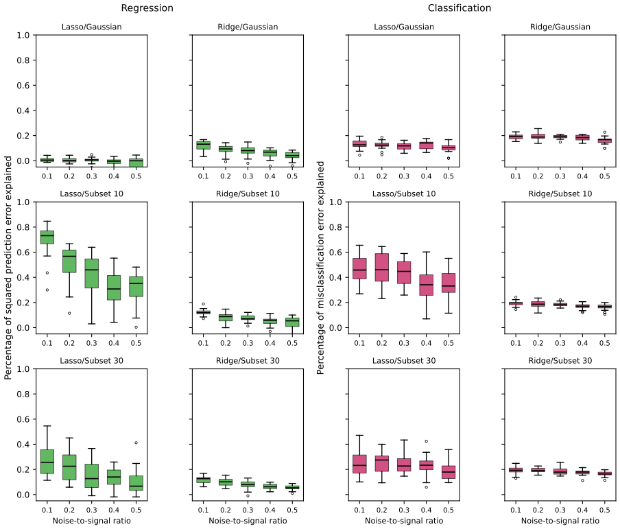
fig_16_2. Reproduces Hastie, Tibshirani and Friedman (2009), Figure 16.2. Download: PDF · SVGNote on the book: the noise-to-signal ratio of the classification problems
The book defines \(\NSR=\Var(Y\given\eta(X))/\Var(\eta(X))\) for both problems. For regression this is unambiguous. For classification, read literally (signal = the variance of the logit \(\eta\), noise = the average Bernoulli variance \(\E[p(1-p)]\)), an NSR of 0.1 forces \(\Var\eta\approx1.85\), a Bayes error of 0.28 and so at most 44% of the coin-flip error can be explained; ten simulated data sets then give medians of only about 0.12 (lasso) and 0.07 (ridge) for the 10-sparse model, far below the book's boxes. Taking the signal on the same scale as the noise, \(\Var p(X)=\Var\E(Y\given X)\) (exactly the regression definition, since there \(\E(Y\given X)=\eta\)), an NSR of 0.1 means \(\Var\eta\approx305\) and a Bayes error of 0.03, and the simulation then reproduces the book's classification panels closely (Figure 16.2 above). We therefore use \(\NSR=\E[p(1-p)]/\Var(p)\), solved for the scale of \(\eta\) by bisection (the expectations are one-dimensional integrals over \(\eta\); because \(p\) is nearly a step function when \(\Var\eta\) is large, they need a fine grid rather than a Gauss–Hermite rule, which overstates the ratio by a third at \(\Var\eta=175\)).
The L2 penalty does poorly everywhere; the lasso does reasonably well in the two sparse scenarios, worse as the noise grows and as the truth gets denser; classification differences are less marked than regression ones. A body of theory supports L1 estimation for sparse problems (Donoho and Johnstone, 1994; Donoho and Elad, 2003; Donoho, 2006; Candès and Tao, 2007); Result 16.5 is its simplest instance.
16.2.3 Regularization Paths, Over-fitting and Margins
pp. 613–616 Boosting is often said not to overfit, or more precisely to be slow to overfit. Part of the reason is that misclassification error is less sensitive to variance than squared error. This section shows that the regularisation paths of boosted models are well behaved, and have an appealing limit for some losses.
The block-correlated simulation (Exercise 16.1): a dictionary of 1000 Gaussian variables, correlated with \(\rho=0.95\) within 50 blocks of 20 variables each and uncorrelated between blocks; one variable per block has a nonzero standard Gaussian coefficient; Gaussian noise gives a noise-to-signal ratio of 0.72; \(N=60\). The grouping imitates the strong correlations between nearby trees, so FS0 on this dictionary is an idealised gradient boosting with shrinkage. Both paths are piecewise linear and computed exactly.
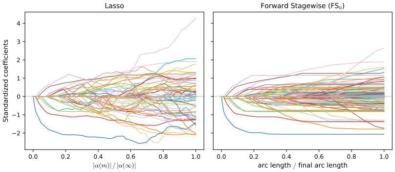
block_data(seed=1). Code: fig_16_3. Reproduces Hastie, Tibshirani and Friedman (2009), Figure 16.3. Download: PDF · SVG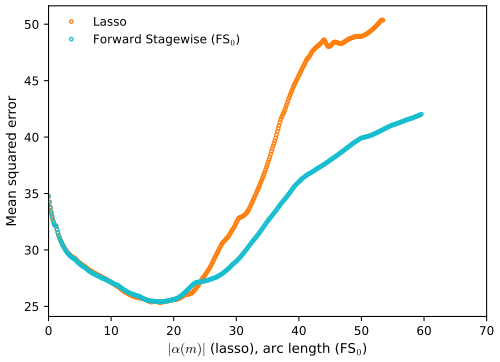
fig_16_4. Reproduces Hastie, Tibshirani and Friedman (2009), Figure 16.4. Download: PDF · SVGThe coefficient profiles agree early; later the stagewise ones are monotone and smoother while the lasso's fluctuate, a consequence of the near-collinearity within blocks (the lasso cannot decide how to share weight between near-copies, Exercise 3.28). The test errors are similar over the useful part of the path, and stagewise takes longer to overfit, plausibly because its path is smoother.
FS0 is a monotone lasso (Hastie et al., 2007). Let \(\cT^a=\cT\cup\{-\cT\}\) be the augmented dictionary with a negated copy of every basis function, and consider \(f(x)=\sum_{T_k\in\cT^a}\alpha_kT_k(x)\) with \(\alpha_k\ge0\). In this space the lasso coefficient paths are non-negative and those of FS0 are non-decreasing. The monotone lasso path is characterised by the differential equation
\[ \frac{\partial\ba}{\partial\ell}=\rho^{ml}(\ba(\ell)), \tag{16.6} \]with \(\ba(0)=0\) and \(\ell\) the L1 arc length of the path (Exercise 16.2); its velocity \(\rho^{ml}\ge0\) decreases the loss at the optimal quadratic rate per unit of arc length. The lasso solves a similar equation, except that its direction is optimal per unit increase of the L1 norm; it may therefore have negative components and need not be monotone. Restricting the coefficients to be non-negative is natural in the augmented dictionary, which removes an obvious ambiguity, and matches tree boosting: a new tree is always positively correlated with the current residual.
Result 16.6 (the lasso in the doubled dictionary)
Minimise \(R(\ba^+-\ba^-)+\lambda\sum_k(\alpha^+_k+\alpha^-_k)\) over \(\ba^\pm\ge0\). At any solution \(\alpha^+_k\alpha^-_k=0\) for every \(k\) (when \(\lambda>0\)), and \(\ba=\ba^+-\ba^-\) solves the ordinary lasso; so the non-negative lasso in \(\cT^a\) and the lasso in \(\cT\) have the same solutions, and its L1 norm \(\sum_k(\alpha^+_k+\alpha^-_k)\) equals \(|\ba|_1\).
Proof
If \(\alpha^+_k,\alpha^-_k>0\), subtract \(m=\min(\alpha^+_k,\alpha^-_k)\) from both: the difference, hence the fit \(R\), is unchanged and the penalty falls by \(2\lambda m>0\), contradicting optimality. With \(\alpha^+_k\alpha^-_k=0\), \(\alpha^+_k+\alpha^-_k=|\alpha^+_k-\alpha^-_k|\), so the objective equals the lasso objective at \(\ba=\ba^+-\ba^-\); conversely any \(\ba\) is represented by \(\ba^\pm=\max(\pm\ba,0)\) with the same value. The two minimisations therefore have the same optimal value and corresponding solutions. ∎
Result 16.7 (the direction of FS0: steepest descent per unit arc length, to second order)
Work in \(\cT^a\) with \(\ba\ge0\), squared-error loss \(R=\frac12\|\by-\bT\ba\|^2\) and correlations \(c_k=\langle T_k,\br\rangle\). Moving at unit arc-length speed in a direction \(\bd\ge0\), \(\sum_kd_k=1\), the loss is \(R(\ell)=R-\ell\,\bc^\T\bd+\tfrac12\ell^2\|\bT\bd\|^2\). (a) The first-order rate \(\bc^\T\bd\) is maximal, equal to \(C=\max_kc_k\), exactly for directions supported on the tied set \(\mathcal A=\{k:c_k=C\}\). (b) Among those, the one minimising the second-order term \(\|\bT\bd\|^2\) is characterised by \(\langle T_k,\bT\bd\rangle=\mu\) where \(d_k>0\) and \(\ge\mu\) where \(d_k=0\), \(k\in\mathcal A\): this is the sign-constrained least-squares direction of FS0 (Filling the gap 3.14), rescaled to unit arc length. Since it has \(\bd\ge0\), the FS0 path is non-decreasing in \(\cT^a\).
Proof
Expanding \(\frac12\|\br-\ell\bT\bd\|^2\) gives the formula for \(R(\ell)\). (a) \(\bc^\T\bd\le C\sum_kd_k=C\), with equality iff \(d_k=0\) whenever \(c_k\lt C\). (b) Minimise the convex \(\frac12\bd^\T\bT_\mathcal A^\T\bT_\mathcal A\bd\) subject to \(\bd\ge0\), \(\bone^\T\bd=1\). The Karush–Kuhn–Tucker conditions with multipliers \(\mu\) (equality) and \(\nu_k\ge0\) (bounds) are \[\bT_\mathcal A^\T\bT_\mathcal A\bd=\mu\bone+\boldsymbol\nu\], \(\nu_kd_k=0\): exactly the stated conditions. The FS0 direction is \[\bc^*=\argmin_{\bc\ge0}\frac12\bc^\T\bT_\mathcal A^\T\bT_\mathcal A\bc-\bone^\T\bc\] (the non-negative least-squares fit of the residual on the tied, sign-adjusted columns, written with the Gram matrix since \(\bT_\mathcal A^\T\br=C\bone\)), whose conditions are \[\bT_\mathcal A^\T\bT_\mathcal A\bc^*=\bone+\boldsymbol\nu'\], \(\nu'_k\ge0\), \(\nu'_kc^*_k=0\). So \(\bd=\bc^*/\bone^\T\bc^*\) satisfies (b) with \(\mu=1/\bone^\T\bc^*\). Along the direction, the correlations of moving variables fall at the common rate \(\mu\) and the other tied ones at least as fast, so the tie (and first-order optimality) is kept for a positive stretch; the direction is recomputed when a new variable ties. ∎
In the original dictionary FS0 can still reverse a coefficient, by later increasing the coefficient of the negated copy; its arc length then exceeds its L1 norm. On the data of Figure 16.3 this never happens; on the 200-input data of the demonstration it happens 11 times, each time by a tiny amount, against 501 reversals for the lasso.
Margins. It has been suggested that boosting works well for two-class problems because, like the support vector machine (Section 4.5.2 and Chapter 12), it maximises a margin. Schapire et al. (1998) define the normalised L1 margin of \(f(x)=\sum_k\alpha_kT_k(x)\) as
\[ m(f)=\min_i\frac{y_if(x_i)}{\sum_{k=1}^K|\alpha_k|}, \tag{16.7} \]the minimum taken over the training sample, \(y_i\in\{-1,+1\}\). Unlike the L2 margin (4.40) of the support vector machine, it measures distance in L∞ units.
Result 16.8 (the L1 margin is an L∞ distance)
Map each point to its vector of basis-function values \(h(x)=(T_1(x),\dots,T_K(x))\in\R^K\). The L∞ distance from \(h\) to the hyperplane \(H=\{u:\ba^\T u=0\}\) is \(|\ba^\T h|/\|\ba\|_1\). Hence \(y_if(x_i)/|\ba|_1\) is the signed L∞ distance from \(h(x_i)\) to the decision boundary, and \(m(f)\) is the L∞ distance from the boundary to the closest training point (negative if a point is misclassified). Margin and training error are linked trivially: \(m(f)>0\) if and only if every training point is classified correctly.
Proof
For \(u\in H\), \(|\ba^\T h|=|\ba^\T(h-u)|\le\|\ba\|_1\|h-u\|_\infty\) (Hölder), so the distance is at least \(|\ba^\T h|/\|\ba\|_1\). The point \(u=h-t\,\sgn(\ba)\) with \(t=\ba^\T h/\|\ba\|_1\) lies in \(H\) (since \(\ba^\T\sgn(\ba)=\|\ba\|_1\)) at L∞ distance \(|t|\), so the bound is attained. The L1 norm is dual to the L∞ norm, just as the Euclidean norm is self-dual for the support vector margin. ∎
Schapire et al. (1998) prove that with separable data AdaBoost increases \(m(f)\) at every iteration; Rätsch and Warmuth (2002) prove that AdaBoost with shrinkage converges asymptotically to an L1-margin-maximising solution; Rosset et al. (2004) show that the solutions of (16.2) with a general loss converge, as \(\lambda\downarrow0\), to a margin-maximising configuration for particular losses, among them the exponential loss and the binomial deviance. The core of that argument is short:
Result 16.9 (the exponential loss with a vanishing L1 penalty maximises the margin)
Let the data be separable by the dictionary: \(m^*=\max_{|\ba|_1=1}\min_iy_i\ba^\T h(x_i)>0\). Let \(\hat\ba(t)\) minimise \(L(\ba)=\sum_ie^{-y_i\ba^\T h(x_i)}\) subject to \(|\ba|_1\le t\). Then \(\bar\ba(t)=\hat\ba(t)/|\hat\ba(t)|_1\) satisfies \(m(\bar\ba(t))\ge m^*-\log N/|\hat\ba(t)|_1\) and \(|\hat\ba(t)|_1\to\infty\); hence \(m(\bar\ba(t))\to m^*\) as \(t\to\infty\), and every limit point of \(\bar\ba(t)\) is an L1-margin maximiser.
Proof
Let \(\ba^*\) attain \(m^*\) with \(|\ba^*|_1=1\). Then \(t\ba^*\) is feasible and \(L(t\ba^*)\le Ne^{-tm^*}\). Write \(s=|\hat\ba(t)|_1\le t\). The loss is at least its largest term, \(L(\hat\ba(t))\ge e^{-s\,m(\bar\ba(t))}\). Optimality gives \(e^{-s\,m(\bar\ba)}\le Ne^{-tm^*}\), i.e. \(s\,m(\bar\ba)\ge tm^*-\log N\). The left side is at most \(s\) (margins of a unit-L1 combination of functions bounded by 1 are at most 1, with trees scaled to sup norm 1), so \(s\ge tm^*-\log N\to\infty\). Dividing by \(s\) and using \(t\ge s\): \[m(\bar\ba)\ge(t/s)m^*-\log N/s\ge m^*-\log N/s\to m^*\]. The margin is continuous in \(\ba\), so limit points attain \(m^*\). ∎
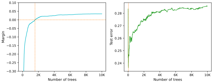
fig_16_5. Reproduces Hastie, Tibshirani and Friedman (2009), Figure 16.5. Download: PDF · SVGCollecting the section: the sequence of boosted classifiers forms an L1-regularised monotone path to a margin-maximising solution. The margin-maximising end can be a very poor, overfitted solution, as in Figure 16.5; early stopping chooses a point along the path and should use validation data.
See also (companion course): early stopping as regularisation, Result 9.7.
16.3 Learning Ensembles
pp. 616–617 The insights of Section 16.2 suggest a more efficient way to build an ensemble. Consider again functions of the form
\[ f(x)=\alpha_0+\sum_{T_k\in\cT}\alpha_kT_k(x), \tag{16.8} \]with \(\cT\) a dictionary of basis functions, typically trees. Gradient boosting and random forests produce models with thousands of trees, and boosting with shrinkage fits an L1-regularised monotone path in this space. Friedman and Popescu (2003) split the process into two explicit stages:
- a finite dictionary \(\cT_L=\{T_1(x),\dots,T_M(x)\}\) of basis functions is induced from the training data;
- a family of functions \(f_\lambda(x)\) is built by fitting a lasso path in this dictionary:
In the simplest form, (16.9) post-processes the trees of a boosting run or a random forest: the lasso keeps a much smaller set, saving computation and storage at prediction time. Unlike stacking (Section 8.8), which weights a few models fitted to the same data by least squares on cross-validated predictions, here the weights of hundreds of base learners are fitted to their in-sample outputs and the penalty does the regularising.
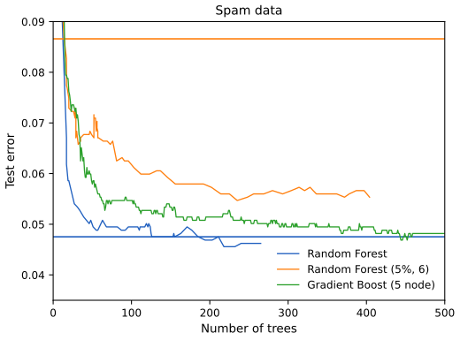
fig_16_6. Reproduces Hastie, Tibshirani and Friedman (2009), Figure 16.6. Download: PDF · SVGAs in the book, post-processing improves on the random forest only modestly (0.0475 to 0.0456) but keeps fewer than half of its first 500 trees, and its best error is close to that of gradient boosting. The forest of shallow trees grown on 5% subsamples, about a hundred times cheaper to build, is a poor ensemble when its trees are simply averaged (0.087), and there post-processing helps dramatically (0.055), though it stays behind the full forest. The book reports about 40 trees for the post-processed forest; our lasso path reaches its minimum later, at 218 trees (with 150 trees it equals the forest's error).
16.3.1 Learning a Good Ensemble
pp. 617–620 Not every dictionary post-processes well: we want basis functions that cover the space where they are needed and that differ enough from each other for the lasso to make use of them. Friedman and Popescu (2003) borrow from numerical quadrature and importance sampling. Write the unknown function as an integral
\[ f(x)=\int\beta(\gamma)\,b(x;\gamma)\,d\gamma, \tag{16.10} \]where \(\gamma\in\Gamma\) indexes the basis functions \(b(x;\gamma)\) (for trees: split variables, split points and leaf values). Numerical quadrature chooses points \(\gamma_m\) and weights \(\alpha_m\) so that \(f_M(x)=\alpha_0+\sum_{m=1}^M\alpha_mb(x;\gamma_m)\) approximates \(f\) over the domain of \(x\); importance sampling draws the \(\gamma_m\) at random but more often where they matter. The (lack of) relevance of \(\gamma\) is measured with the loss of (16.9):
\[ Q(\gamma)=\min_{c_0,c_1}\sum_{i=1}^NL(y_i,\,c_0+c_1b(x_i;\gamma)), \tag{16.11} \]evaluated on the training data. A single basis function would be the global minimiser \(\gamma^*=\argmin_\gamma Q(\gamma)\); random selection necessarily gives \(Q(\gamma)\ge Q(\gamma^*)\), and the characteristic width of a sampling scheme \(\mathcal S\) is
\[ \sigma=\E_\mathcal S[Q(\gamma)-Q(\gamma^*)]. \tag{16.12} \]Too narrow a scheme gives many near-copies of \(b(x;\gamma^*)\); too wide a scheme gives diverse but mostly irrelevant basis functions.
Filling the gap 16.3: what (16.10)–(16.11) mean for squared error, and why random sampling with refitted weights is quadrature pp. 618–619
(a) For squared-error loss, \[Q(\gamma)=\sum_i(y_i-\bar y)^2\,\big(1-\hat\rho^2_\gamma\big)\], with \(\hat\rho_\gamma\) the sample correlation between \(y\) and \(b(x;\gamma)\): a basis function is relevant exactly to the extent that it is correlated with the response, and \[Q(\gamma)-Q(\gamma^*)=\sum_i(y_i-\bar y)^2(\hat\rho^2_{\gamma^*}-\hat\rho^2_\gamma)\].
(b) For any density \(r\) on \(\Gamma\) that is positive where \(\beta\ne0\), \(f(x)=\E_r\big[\beta(\gamma)b(x;\gamma)/r(\gamma)\big]\), so with \(\gamma_1,\dots,\gamma_M\) drawn from \(r\) the average \(\frac1M\sum_m\beta(\gamma_m)b(x;\gamma_m)/r(\gamma_m)\) is unbiased for \(f(x)\) with variance \(\Var_r[\beta b/r]/M\), smallest when \(r\) puts its mass where \(|\beta(\gamma)b(x;\gamma)|\) is large. The weights \(\beta(\gamma_m)/(Mr(\gamma_m))\) are unknown, which is why (16.9) estimates them: the lasso is the "quadrature rule" fitted to the data.
Derivation
(a) For fixed \(\gamma\), (16.11) is a simple linear regression of \(y\) on \(b_i=b(x_i;\gamma)\), whose residual sum of squares is \(S_{yy}-S_{by}^2/S_{bb}=S_{yy}(1-\hat\rho^2)\) with \(S_{yy}=\sum(y_i-\bar y)^2\), \(S_{bb}=\sum(b_i-\bar b)^2\), \(S_{by}=\sum(b_i-\bar b)(y_i-\bar y)\) (if \(b\) is constant on the sample, \(Q=S_{yy}\)). (b) \(\E_r[\beta b/r]=\int r\,\beta b/r\,d\gamma=f(x)\), and the variance of an average of \(M\) independent copies is the single-draw variance over \(M\). By Cauchy–Schwarz, \[\E_r[(\beta b/r)^2]\ge(\E_r|\beta b/r|)^2=(\int|\beta b|)^2\], with equality when \(r\propto|\beta b|\). ∎
Friedman and Popescu use subsampling to introduce randomness, which gives their ensemble generator:
Algorithm 16.2 (ISLE ensemble generation) p. 619
- \(f_0(x)=\argmin_c\sum_{i=1}^NL(y_i,c)\).
- For \(m=1\) to \(M\):
- \[\gamma_m=\argmin_\gamma\sum_{i\in S_m(\eta)}L\big(y_i,\,f_{m-1}(x_i)+b(x_i;\gamma)\big)\];
- \(f_m(x)=f_{m-1}(x)+\nu\,b(x;\gamma_m)\).
- \[\cT_{ISLE}=\{b(x;\gamma_1),b(x;\gamma_2),\dots,b(x;\gamma_M)\}\].
\(S_m(\eta)\) is a subsample of \(N\cdot\eta\) training observations, \(\eta\in(0,1]\), usually drawn without replacement. In practice step 2(a) is done as in gradient boosting: a tree fitted by least squares to the negative gradient on \(S_m\), with leaf values re-optimised for the loss.
Their simulations suggest \(\eta\le\frac12\), and \(\eta\sim1/\sqrt N\) for large \(N\). Smaller \(\eta\) means more randomness and a wider \(\sigma\). The memory parameter \(\nu\in[0,1]\) makes later basis functions avoid those already found: the larger \(\nu\), the more the procedure looks for something new. Familiar schemes are special cases:
- Bagging: \(\eta=1\), sampling with replacement, \(\nu=0\) (then \(f_{m-1}=f_0\) for every \(m\), so every tree is fitted to \(y-f_0\) on its own bootstrap sample). Friedman and Hall (2007) argue that sampling half the data without replacement is equivalent to a bootstrap sample, and much cheaper (Filling the gap 16.4).
- Random forests: similar, with extra randomness from the random choice of split variables. Reducing \(\eta\lt\frac12\) in Algorithm 16.2 has an effect similar to reducing \(m\) in random forests without its potential biases (the book's Section 15.4.2).
- Gradient boosting with shrinkage (10.41): \(\eta=1\), which usually does not give enough width.
- Stochastic gradient boosting (Friedman, 1999; Section 10.12.2) follows the recipe exactly.
The recommended values are \(\nu=0.1\) and \(\eta\le\frac12\); ensemble generation followed by lasso post-processing is called an importance sampled learning ensemble (ISLE).
Filling the gap 16.4: half-samples without replacement against bootstrap samples p. 619
For the simplest statistic, the mean, a half-sample drawn without replacement and a bootstrap sample give the same variability to first order: with \(s^2=\frac1N\sum_i(y_i-\bar y)^2\), the variance (over resampling) of the mean of a bootstrap sample is \(s^2/N\), and that of the mean of a half-sample (\(n=N/2\), without replacement) is \(s^2/(N-1)\). A bootstrap sample contains on average \(1-(1-1/N)^N\approx63.2\%\) distinct observations, some repeated; a half-sample 50%, none repeated, and fitting a tree to it costs half as much.
Derivation
Bootstrap: the \(N\) draws are independent, each with variance \(s^2\), so the mean has variance \(s^2/N\). Without replacement: let \(I_i\) indicate that observation \(i\) is in the subsample, so \(\bar y_S=\frac1n\sum_iI_iy_i\), with \(\E I_i=n/N\), \(\Var I_i=\frac nN(1-\frac nN)\), and for \(i\ne j\), \[\Cov(I_i,I_j)=\frac{n(n-1)}{N(N-1)}-\frac{n^2}{N^2}=-\frac{n(N-n)}{N^2(N-1)}\]. Since \(\sum_iI_i=n\) is fixed we may replace \(y_i\) by \(y_i-\bar y\) (it changes \(\bar y_S\) by a constant); with \(u_i=y_i-\bar y\), \(\sum u_i=0\) and \(\sum_{i\ne j}u_iu_j=-\sum u_i^2\), so \[\Var\big(\sum I_iu_i\big)=\sum u_i^2\big[\frac nN(1-\frac nN)+\frac{n(N-n)}{N^2(N-1)}\big]=\sum u_i^2\,\frac{n(N-n)}{N(N-1)}\]. Dividing by \(n^2\) and using \(\sum u_i^2=Ns^2\): \(\Var\bar y_S=\frac{s^2}{n}\frac{N-n}{N-1}\), which for \(n=N/2\) is \(s^2/(N-1)\). The fraction of distinct observations: each one is missed by all \(N\) bootstrap draws with probability \((1-1/N)^N\to e^{-1}\). ∎
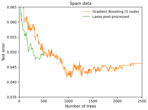
fig_16_7. Reproduces Hastie, Tibshirani and Friedman (2009), Figure 16.7. Download: PDF · SVGAs in the book, post-processing does not improve the prediction error here (its best, 0.0475, is close to the boosted model's 0.0462 after 2500 trees and above the boosting minimum 0.0417), but it uses far fewer trees: 325 against 2500, roughly the book's factor of five. In practice the penalty \(\lambda\) of (16.9) would be chosen by cross-validation; showing the whole path on the test data only displays what post-processing can do.
A regression example. The model
\[ f(X)=10\cdot\prod_{j=1}^5e^{-2X_j^2}+\sum_{j=6}^{35}X_j, \tag{16.13} \]with \(X\sim U[0,1]^{100}\) (the last 65 inputs are noise) and \(Y=f(X)+\varepsilon\), \(\varepsilon\sim\N(0,\sigma^2)\), \(\sigma=1.3\). The book reports a signal-to-noise ratio of about 2; exactly, since the two terms of (16.13) are independent,
\[ \Var f(X)=100\Big[\Big(\int_0^1e^{-4x^2}dx\Big)^5-\Big(\int_0^1e^{-2x^2}dx\Big)^{10}\Big]+\frac{30}{12}=3.583, \]and \(3.583/1.69=2.12\). There are 1000 training points, and the error \(\E(\hat f(X)-f(X))^2\) is estimated on 500 test points.
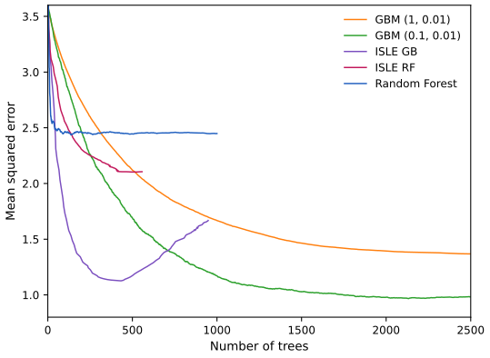
fig_16_8. Reproduces Hastie, Tibshirani and Friedman (2009), Figure 16.8. Download: PDF · SVGSee also (this course): bagging in Section 8.7 and subsampling in boosting in Section 10.12.2; (companion course) Filling the gap 14.3, why bagged models have highly correlated errors.
16.3.2 Rule Ensembles
pp. 622–623 A modification focuses on individual rules (Friedman and Popescu, 2003), like those of PRIM (Section 9.3): each tree of the ensemble is broken into the rules it defines. The book's Figure 16.9 (a drawing, not reproduced) shows a tree whose root (node 0) splits on \(X_1\lt2.1\) into node 1 (a leaf) and node 2; node 2 splits on \(X_3\in\{S\}\) (node 3) against \(X_3\in\{M,L\}\) (node 4, a leaf); node 3 splits on \(X_7\lt4.5\) (node 5) against \(X_7\ge4.5\) (node 6), both leaves. Every node except the root gives a rule, the product of the conditions on the path to it:
\[ \begin{aligned}R_1(X)&=I(X_1\lt2.1)\\R_2(X)&=I(X_1\ge2.1)\\R_3(X)&=I(X_1\ge2.1)\cdot I(X_3\in\{S\})\\R_4(X)&=I(X_1\ge2.1)\cdot I(X_3\in\{M,L\})\\R_5(X)&=I(X_1\ge2.1)\cdot I(X_3\in\{S\})\cdot I(X_7\lt4.5)\\R_6(X)&=I(X_1\ge2.1)\cdot I(X_3\in\{S\})\cdot I(X_7\ge4.5)\end{aligned} \tag{16.14} \]Result 16.10 (the rules of a tree span it, and over-span it; Exercise 16.3)
Rules 1, 4, 5 and 6 are the indicators of the four terminal nodes. A least-squares regression on them reproduces the regression tree (each fitted value is the mean of its leaf), and a logistic regression on them reproduces the classification tree's leaf proportions. The six rules satisfy \(R_1+R_2=1\), \(R_2=R_3+R_4\), \(R_3=R_5+R_6\), so with an intercept they span only a 4-dimensional space: (16.14) is an over-complete basis for the tree.
Proof
A point reaches exactly one terminal node, so \(R_1,R_4,R_5,R_6\) are 0/1 with exactly one equal to 1: the leaf indicators \(L_1,\dots,L_4\), with \(\sum_jL_j=1\). For \(f=\sum_jb_jL_j\), the residual sum of squares splits by leaf, \(\sum_j\sum_{i\in\text{leaf }j}(y_i-b_j)^2\), minimised by \(b_j=\bar y_j\), the leaf mean, exactly the regression tree's fitted value. For the logistic model with logit \(\sum_jb_jL_j\), the log-likelihood also splits by leaf, \(\sum_j[n_{1j}b_j-n_j\log(1+e^{b_j})]\), with stationary point \(e^{b_j}/(1+e^{b_j})=n_{1j}/n_j\), the leaf proportion (when \(0\lt n_{1j}\lt n_j\); a pure leaf sends \(b_j\) to \(\pm\infty\), the logistic version of a proportion of 0 or 1). The identities: a point satisfies either \(X_1\lt2.1\) or \(X_1\ge2.1\); given \(X_1\ge2.1\), either \(X_3\in\{S\}\) or \(X_3\in\{M,L\}\); and so on. They give \(R_2,R_3\) as sums of leaf indicators and \(R_1+R_2\) as the intercept, so the span with intercept is that of the four leaves. ∎
For each tree \(T_m\) of an ensemble build its mini-ensemble of rules \(\cT^m_{RULE}\) and combine them,
\[ \cT_{RULE}=\bigcup_{m=1}^M\cT^m_{RULE}, \tag{16.15} \]then post-process with the lasso as before. Advantages: the space of models is larger, which can improve performance; rules are easier to interpret than trees; and it is natural to add each input \(X_j\) as a linear term, so that linear structure is cheap to represent. Friedman and Popescu (2008) demonstrate the method (RuleFit) on several examples, including (16.13).
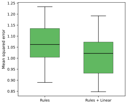
fig_16_10. Reproduces Hastie, Tibshirani and Friedman (2009), Figure 16.10. Download: PDF · SVGThe linear terms help because 30 of the 35 relevant inputs in (16.13) enter linearly, and a linear function is expensive to build from rules. On the training set of Figure 16.8 the rules-plus-linear model, with its penalty chosen by cross-validation, keeps 265 of 2052 terms and reaches a test error of 1.094 (rules alone: 1.188); the book reports 1.06. As the book notes, this is not directly comparable with the curves of Figure 16.8, whose minima are chosen with the test data.
Bibliographic notes. pp. 623–624 Many machine learning methods have been called ensemble methods: neural networks, boosting, bagging, random forests; Dietterich (2000) surveys tree ensembles. Neural networks (Chapter 11) deserve the name perhaps most, since they learn the basis functions (the hidden units) and how to combine them at the same time; Bishop (2006) treats them in detail, with the Bayesian view (MacKay, 1992; Neal, 1996). Support vector machines (Chapter 12) are also ensembles in this sense, with L2-regularised fitting in a high-dimensional feature space; boosting and the lasso exploit sparsity through L1 regularisation, while support vector machines rely on the kernel trick of L2 regularisation. C5.0 (Quinlan, 2004) is a commercial tree and rule generator with goals in common with RuleFit. The large literature on "combining classifiers" has many ad hoc schemes; Kittler et al. (1998) give a principled approach.
Exercises
All 4 exercises of Chapter 16 (Hastie, Tibshirani and Friedman, 2009, p. 624), restated in my own words, with complete solutions (hidden).
Exercise 16.1. Describe exactly how to generate the block-correlated data of Section 16.2.3.
Solution
Fix \(N=60\), \(p=1000\), blocks \(B_1,\dots,B_{50}\) of 20 consecutive variables, \(\rho=0.95\), \(\NSR=0.72\).
- For each observation \(i\) and block \(b\), draw a shared factor \(Z_{ib}\sim\N(0,1)\), and for each \(j\in B_b\) an independent \(E_{ij}\sim\N(0,1)\); set \(X_{ij}=\sqrt\rho\,Z_{ib}+\sqrt{1-\rho}\,E_{ij}\). Then \(\Var X_{ij}=\rho+(1-\rho)=1\), \(\Cov(X_{ij},X_{ik})=\rho\) for \(j\ne k\) in the same block, and 0 across blocks (independent factors). Equivalently, draw the rows from \(\N(\mathbf 0,\Sigma)\) with \(\Sigma\) block diagonal, each block \((1-\rho)\bI+\rho\bone\bone^\T\).
- In each block pick one variable at random and give it a coefficient \(\beta_j\sim\N(0,1)\); all other coefficients are 0.
- The signal variance is \(\Var(X^\T\bb)=\bb^\T\Sigma\bb=\sum_j\beta_j^2\) (one nonzero per block, unit variances). Set \(\sigma^2=0.72\,\bb^\T\Sigma\bb\) and \(y_i=x_i^\T\bb+\sigma\varepsilon_i\), \(\varepsilon_i\sim\N(0,1)\). (Using the sample variance of \(x_i^\T\bb\) instead gives a slightly different, data-dependent \(\sigma\).)
The code's
block_datadoes exactly this; with seed 1 the 60 by 1000 sample has within-block sample correlations averaging 0.95 and between-block ones averaging 0.00, as designed.Exercise 16.2. Let \(\ba(t)\in\R^p\) be continuous and piecewise differentiable with \(\ba(0)=\mathbf 0\), and define its L1 arc length
\[ \Lambda(t)=\int_0^t|\dot\ba(s)|_1\,ds. \tag{16.16} \]Show that \(\Lambda(t)\ge|\ba(t)|_1\), with equality if and only if \(\ba\) is monotone on \([0,t]\).
Solution
For each coordinate, by the fundamental theorem of calculus (valid for continuous, piecewise differentiable functions) \(\alpha_j(t)=\int_0^t\dot\alpha_j(s)\,ds\), so \(|\alpha_j(t)|\le\int_0^t|\dot\alpha_j(s)|ds\). Summing over \(j\) and exchanging sum and integral gives \(|\ba(t)|_1\le\Lambda(t)\). Equality in the sum holds iff it holds for every \(j\), and \(|\int g|=\int|g|\) iff \(g\ge0\) almost everywhere or \(g\le0\) almost everywhere, i.e. iff \(\alpha_j\) is non-decreasing or non-increasing on \([0,t]\). So equality holds iff every coordinate is monotone on \([0,t]\) ("monotone" must be read coordinatewise; different coordinates may move in different directions). This is why FS0's arc length equals its L1 norm while its path is monotone (Figure 16.3: both 59.6), and why the lasso's L1 norm \(|\ba|_1=53.4\) is far below its arc length on the same data. Numerically, for the lasso path of Figure 16.3 the arc length is 133.7, two and a half times its final L1 norm.
Exercise 16.3. Show that a linear regression on rules 1, 4, 5 and 6 of (16.14) gives the same fit as the regression tree, and that the same holds for classification with a logistic regression.
Solution
Result 16.10. The four rules are the leaf indicators, so both regressions fit one free constant per leaf, and their criteria separate over leaves: least squares gives the leaf means, the logistic likelihood the leaf proportions (logits of them), which are the trees' own estimates. Confirmed numerically on data simulated from the tree of Figure 16.9 (500 points, continuous \(X_1,X_7\), a three-level \(X_3\)): the least-squares fit on \(R_1,R_4,R_5,R_6\) equals the leaf means to \(10^{-14}\), the logistic fit (Newton's method) equals the leaf proportions to \(10^{-10}\), and the six rules plus an intercept have rank 4.
Exercise 16.4. Program and run the simulation study of Figure 16.2.
Solution
See Figure 16.2 and Filling the gap 16.2; the code is
bos_simulationin the Python module. The design: for each of the 2 tasks, 3 sparsity levels and 5 noise-to-signal ratios, 20 data sets of 50 observations of 300 independent standard normal inputs; coefficients as described; \(\eta\) scaled to the target NSR (by a closed form for regression, by bisection on the probability-scale NSR for classification, note); lasso and ridge fitted by least squares on the (0/1) response; best test error over each path in closed form. Findings: the lasso dominates in both sparse scenarios (medians 0.73 against 0.12 for regression at NSR 0.1 with 10 nonzero coefficients; 0.46 against 0.20 for classification), ridge is better only with 300 nonzero coefficients, where both explain little (regression: 0.13 against 0.00; classification 0.19 against 0.13), and performance decays with the NSR and with density. The whole study takes a few minutes, almost all of it the classification integrals.
Demonstrations for this chapter
Each demonstration runs in the browser and links back to these notes. The ▶ Demo boxes above open them already set to the case under discussion.
| Demonstration | What you can see | Sections and results |
|---|---|---|
| Forward stagewise against the lasso | The exact lasso path, Algorithm 16.1 with step \(\varepsilon\) and its exact limit FS0, and the test error along both, on the prostate data or on a 200-input block-correlated simulation with adjustable correlation. Presets: 1 prostate (Figure 16.1); 2 correlated blocks (Figure 16.3); 3 test error (Figure 16.4); 4 independent inputs; 5 a coarse step. | 16.2.1, 16.2.3; Results 16.2–16.4, 16.7; Exercises 16.1, 16.2 |
| Bet on sparsity | The simulation of Figure 16.2 for \(k=1\) to 300 nonzero coefficients: the best error explained by the lasso and by ridge on every simulated data set, regression or classification, any noise-to-signal ratio. Presets: 1 regression; 2 dense truth; 3 noisier; 4 classification; 5 noisy classification. | 16.2.2; Result 16.5, Filling the gap 16.2; Exercise 16.4 |
| Post-processing a tree ensemble with the lasso | Algorithm 16.2 on (16.13) with any subsample fraction, memory, tree size, split-variable sampling and number of trees, then the lasso path (16.9) on the trees: test error of both against the number of trees, and the weight the lasso gives each tree. Presets: 1 boosting; 2 stochastic boosting; 3 bagging-type trees; 4 very slow learning; 5 stumps. | 16.3, 16.3.1; Algorithm 16.2, Filling the gaps 16.3–16.4 |
Related demonstrations: in this course, the least angle regression demo, the bagging demo and the gradient boosting demo; in the companion courses, the trees and committees demo and the L1 versus L2 paths demo. The Python code that produces every figure of this page is code/ch16_ensemble_learning.py (see the code index).
References
- Hastie, T., Tibshirani, R. and Friedman, J. (2009). The Elements of Statistical Learning: Data Mining, Inference, and Prediction, 2nd edition. Springer, New York. Chapter 16, pp. 605–624. hastie.su.domains/ElemStatLearn.
- Bishop, C. M. (2006). Pattern Recognition and Machine Learning. Springer, New York.
- Candès, E. and Tao, T. (2007). The Dantzig selector: statistical estimation when p is much larger than n. The Annals of Statistics, 35(6), 2313–2351.
- Copas, J. B. (1983). Regression, prediction and shrinkage (with discussion). Journal of the Royal Statistical Society, Series B, 45(3), 311–354.
- Dietterich, T. G. (2000). Ensemble methods in machine learning. In Multiple Classifier Systems, Lecture Notes in Computer Science 1857, 1–15. Springer.
- Dietterich, T. G. and Bakiri, G. (1995). Solving multiclass learning problems via error-correcting output codes. Journal of Artificial Intelligence Research, 2, 263–286.
- Donoho, D. L. (2006). For most large underdetermined systems of equations, the minimal L1-norm solution is the sparsest solution. Communications on Pure and Applied Mathematics, 59(7), 907–934.
- Donoho, D. L. and Elad, M. (2003). Optimally sparse representation in general (nonorthogonal) dictionaries via L1 minimization. Proceedings of the National Academy of Sciences, 100(5), 2197–2202.
- Donoho, D. L. and Johnstone, I. M. (1994). Ideal spatial adaptation by wavelet shrinkage. Biometrika, 81(3), 425–455.
- Efron, B., Hastie, T., Johnstone, I. and Tibshirani, R. (2004). Least angle regression (with discussion). The Annals of Statistics, 32(2), 407–499.
- Friedman, J. H. (1999). Stochastic gradient boosting. Technical report, Stanford University; published in Computational Statistics and Data Analysis, 38(4), 367–378 (2002).
- Friedman, J. H. and Hall, P. (2007). On bagging and nonlinear estimation. Journal of Statistical Planning and Inference, 137(3), 669–683.
- Friedman, J., Hastie, T., Rosset, S., Tibshirani, R. and Zhu, J. (2004). Discussion of three boosting papers. The Annals of Statistics, 32(1), 102–107.
- Friedman, J. H. and Popescu, B. E. (2003). Importance sampled learning ensembles. Technical report, Department of Statistics, Stanford University.
- Friedman, J. H. and Popescu, B. E. (2008). Predictive learning via rule ensembles. The Annals of Applied Statistics, 2(3), 916–954.
- Hastie, T., Taylor, J., Tibshirani, R. and Walther, G. (2007). Forward stagewise regression and the monotone lasso. Electronic Journal of Statistics, 1, 1–29.
- James, G. and Hastie, T. (1998). The error coding method and PICTs. Journal of Computational and Graphical Statistics, 7(3), 377–387.
- Kittler, J., Hatef, M., Duin, R. and Matas, J. (1998). On combining classifiers. IEEE Transactions on Pattern Analysis and Machine Intelligence, 20(3), 226–239.
- MacKay, D. J. C. (1992). A practical Bayesian framework for backpropagation networks. Neural Computation, 4(3), 448–472.
- Neal, R. M. (1996). Bayesian Learning for Neural Networks. Springer, New York.
- Neal, R. M. and Zhang, J. (2006). High dimensional classification with Bayesian neural networks and Dirichlet diffusion trees. In Feature Extraction: Foundations and Applications, 265–296. Springer.
- Quinlan, J. R. (2004). C5.0. Rulequest Research.
- Rätsch, G. and Warmuth, M. K. (2002). Maximizing the margin with boosting. In Computational Learning Theory (COLT 2002), Lecture Notes in Computer Science 2375, 334–350. Springer.
- Rosset, S., Zhu, J. and Hastie, T. (2004). Boosting as a regularized path to a maximum margin classifier. Journal of Machine Learning Research, 5, 941–973.
- Schapire, R. E., Freund, Y., Bartlett, P. and Lee, W. S. (1998). Boosting the margin: a new explanation for the effectiveness of voting methods. The Annals of Statistics, 26(5), 1651–1686.
The numerical statements in the text (the path algorithms and their agreement with standard implementations, the stagewise-lasso identities, the risk bounds, the exact test-error formulas, the margin and linear-programming values, the subsampling variances, the rule identities, and every number quoted from the reproduced figures) were confirmed numerically.