Chapter 9. Multivariate methods for heterogeneous data
Many biological objects come without coordinates: we can say how different two cells, two communities or two colours are, but not where they sit in a vector space. Other data mix a large continuous table with a few factors (batches, days, diets), or arrive as counts in a contingency table, or as several tables measured on the same samples. This chapter, following Holmes and Huber (2019), Chapter 9, builds maps for all of these: multidimensional scaling from distances, correspondence analysis for counts, nonlinear embeddings for gradients and trajectories, and the RV coefficient, canonical correlation and its sparse and constrained versions for several tables at once.
Ch. 1 Discrete data Ch. 2 Statistical modeling Ch. 3 Data visualization Ch. 4 Mixture models Ch. 5 Clustering Ch. 6 Testing Ch. 7 Multivariate analysis Ch. 8 Count data and GLMs Ch. 9 Heterogeneous data Ch. 10 Networks and trees Ch. 11 Image data Ch. 12 Supervised learning Ch. 13 Experimental design
How to read these notes
They follow the book. Sections carry the book's numbers (9.2, 9.4.2, ...), the displayed equations that appear in the book keep its numbers, e.g. (9.1), and every figure is the book's figure with the same number, recomputed from the data by the course's R code. The book is applied: it shows what the methods do and leaves the mathematics out. Wherever it states a result without proof, an orange Filling the gap box gives the full argument. Derivations start hidden: open one with its bar, or use the button below.
Questions and exercises. The book's in-text questions appear where they are asked, with short answers. Its eight end-of-chapter exercises are restated, with worked solutions, in the Exercises section; Figures 9.35 to 9.41 belong to those solutions.
Numbers. Every numerical statement made below (eigenvalues, percentages, test statistics, the identities proved in the gap boxes) is verified numerically, and the demonstrations reproduce the R values.
Main reference
S. Holmes and W. Huber, Modern Statistics for Modern Biology, Cambridge University Press (2019), Chapter 9, "Multivariate methods for heterogeneous data". Section, equation, figure, question and exercise numbers below refer to this book. The explanations, derivations and code here are my own; original papers are cited where a result comes from them.
The chapter at a glance
- 9.2 Classical multidimensional scaling (MDS, principal coordinates) turns an \(n\times n\) distance matrix into coordinates: double-centre the squared distances, take eigenvectors. It is exact when the distances are Euclidean (Young and Householder), and optimal in a least-squares sense otherwise. Nonmetric MDS keeps only the rank order of the distances and minimises Kruskal's stress.
- 9.3 Factors such as batch or day enter a PCA as supplementary points (group barycentres). A PCA of rank-transformed Phylochip data exposes a day effect; ComBat removes batch effects with an empirical Bayes location and scale model.
- 9.4 Correspondence analysis (CA) is the SVD of the table of standardised Pearson residuals: the chi-square statistic divided by \(n\) is the sum of the squared singular values, and the biplot shows which rows and columns attract each other.
- 9.5 A hidden gradient (time, a lakeshore, a developmental path) makes the points of a CA or MDS map lie on an arch, the horseshoe; it comes from the cosine shape of the eigenvectors. Kernel MDS and t-SNE represent local distances faithfully and give up on large ones.
- 9.6 Several tables on the same samples: the Mantel and RV coefficients measure global association (with permutation tests), canonical correlation finds maximally correlated linear combinations (and overfits badly when there are more variables than samples), sparse CCA adds \(\ell_1\) constraints, and constrained correspondence analysis restricts CA axes to the span of covariates.
Notation. \(n\) objects (samples, cells, cities); \(\mathbf{X}\) an \(n\times p\) data matrix with rows \(\mathbf{x}_i^\T\); \(\one\) the vector of ones; \(\mathbf{H}\)
Prerequisites. The singular value decomposition and PCA (Chapter 7 of the book), the chi-square test of independence (Chapter 2), distances between objects (Chapter 5), and permutation tests (Chapter 6).
9.2 Multidimensional scaling and ordination
Section 9.2 Sometimes the data are not points in a feature space but a table of (dis)similarities between objects: drugs, images, trees, sequences, microbial communities. Chapter 5 clustered such objects; here the aim is a map, a low-dimensional configuration of points whose Euclidean distances reproduce the given ones as well as possible, much as the first principal plane of a PCA summarises a data table.
Definition 9.1 (distance matrix, Euclidean distance matrix) Section 9.2
A dissimilarity matrix is a symmetric \(n\times n\) matrix \(\mathbf{D}=(d_{ij})\) with \(d_{ij}\ge0\) and \(d_{ii}=0\). It is a distance matrix (metric) if in addition it satisfies the triangle inequality. It is Euclidean if there are points \(\mathbf{x}_1,\dots,\mathbf{x}_n\) in some \(\R^r\) with \(d_{ij}=\|\mathbf{x}_i-\mathbf{x}_j\|\) for all \(i,j\); the smallest such \(r\) is its embedding dimension.
The book's first example uses the great-circle distances, in kilometres, between 33 places in Ukraine. Figure 9.1 is a heatmap of the matrix, with rows and columns reordered by hierarchical clustering; the blocks are regions (the west, the east, Crimea and the south coast).
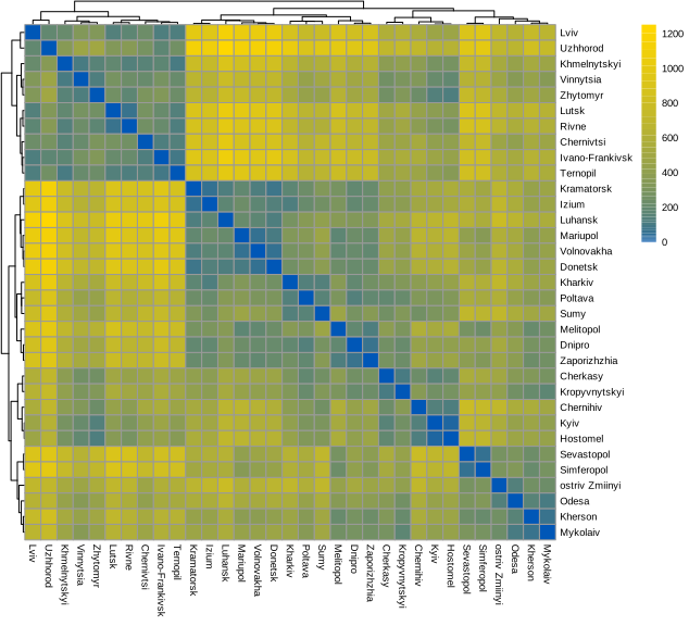
fig_9_1. Download: PDF · SVGClassical MDS (R's cmdscale) returns coordinates and the eigenvalues of a matrix built from the distances (Result 9.1 below). Their bar chart, the screeplot, shows how many dimensions the configuration needs: here two eigenvalues dominate (Figure 9.2), as they should for places on a map.
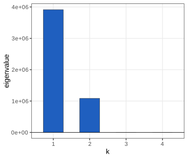
fig_9_2. Download: PDF · SVGQuestion 9.1 (all the eigenvalues)
Look at all 33 eigenvalues returned by cmdscale. What do you notice?
Answer
The first two are \(3.91\times10^6\) and \(1.08\times10^6\), the third is about 342, and two eigenvalues are clearly negative: about \(-358\) and \(-885\) (the remaining ones, of size \(10^{-1}\) to \(10^{-10}\), are rounding). In PCA every eigenvalue is a variance and cannot be negative. In MDS the eigenvalues belong to the double-centred matrix \(\mathbf{B}\) of (9.1), which is positive semi-definite exactly when the distances are Euclidean (Theorem 9.2). Great-circle distances are measured along the curved surface of the Earth, so no configuration of points in any \(\R^r\) reproduces them exactly, and negative eigenvalues are the symptom. They are small here because the country is small compared with the Earth's radius (Figure 9.3 shows them as red bars, too short to see at this scale).
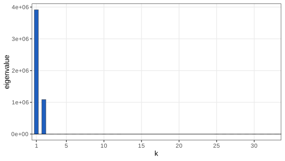
fig_9_3. Download: PDF · SVGThe coordinates of the first two eigenvectors give the map of Figure 9.4. Distances do not change under rotations and reflections, so the map is determined only up to these: cmdscale happened to put Crimea at the top. Flipping the second axis (Figure 9.5) gives the familiar orientation, to be compared with the true longitudes and latitudes (Figure 9.6).
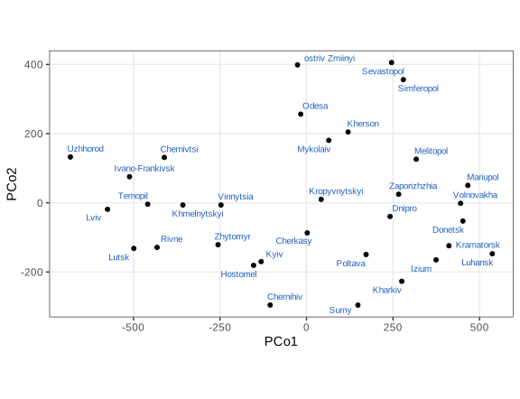
fig_9_4. Download: PDF · SVG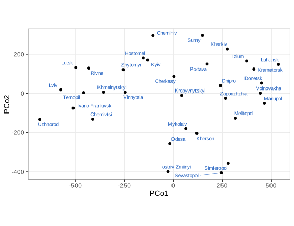
fig_9_5. Download: PDF · SVG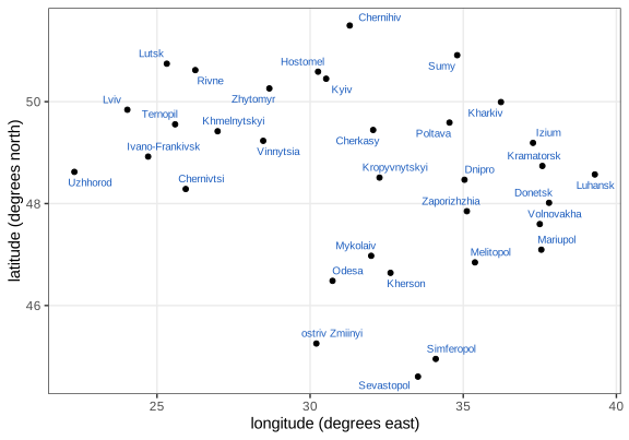
fig_9_6. Download: PDF · SVGQuestion 9.2 (the right aspect ratio)
What aspect ratio should Figure 9.6 have?
Answer
On a sphere of radius \(R=6371\) km, one degree of latitude is always \(2\pi R/360\approx111.2\) km. One degree of longitude at latitude \(\varphi\) is a degree of a circle of radius \(R\cos\varphi\), so it is \(111.2\cos\varphi\) km: 111 km at the equator, nothing at the poles. Ukraine lies between about 44.4° and 52.4° N, where \(\cos\varphi\) runs from 0.71 to 0.61, so no single ratio is right everywhere. Taking the middle, \(\varphi=48^\circ\), one unit on the latitude axis should be drawn \(1/\cos48^\circ=1.49\) times as long as one unit on the longitude axis, which is coord_fixed(1/cos(48*pi/180)) in Figure 9.7. (Note the conversion to radians: R's trigonometric functions take radians.)
Question 9.3 (borders)
Add the international border to Figure 9.6.
Answer
The maps package provides the outline as a polygon (map_data("world", region = "Ukraine")); draw it with geom_polygon under the points and fix the aspect ratio as in Question 9.2. The result is Figure 9.7; the code is fig_9_7 in the chapter's R script.
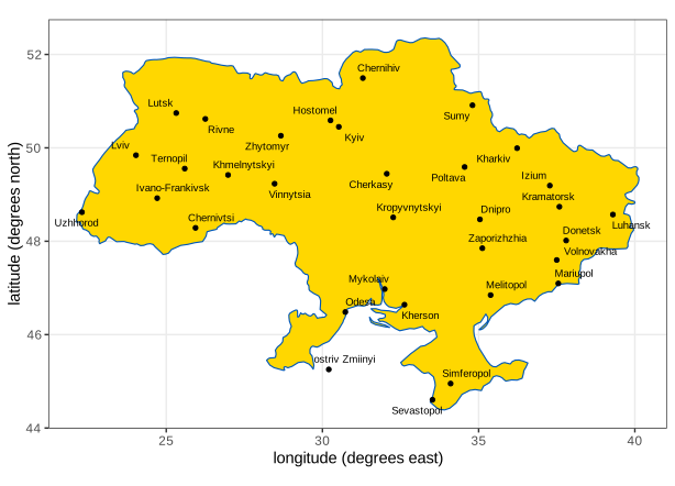
fig_9_7. Download: PDF · SVGA caution from the book: unlike PCA, MDS has only one set of points. There are no variables, so no loadings and no biplot; to interpret the axes one looks at the objects at their extremes.
9.2.1 How does the method work?
Section 9.2.1 Suppose first that the distances come from known points: \(\mathbf{X}\) is \(n\times p\) and \(d_{ij}^2=\sum_k(x_{ik}-x_{jk})^2\). Distances do not depend on where the origin is, so the best we can hope to recover is the centred configuration \(\mathbf{H}\mathbf{X}\) (the columns of \(\mathbf{X}\) minus their means). Its Gram matrix \(\mathbf{B}\)
Result 9.1 (from squared distances to inner products) Section 9.2.1, (9.1), Question 9.4
If \(d_{ij}=\|\mathbf{x}_i-\mathbf{x}_j\|\) then
\[ -\tfrac12\,\mathbf{H}(\mathbf{D}\bullet\mathbf{D})\mathbf{H}=\mathbf{B}=(\mathbf{H}\mathbf{X})(\mathbf{H}\mathbf{X})^\T. \tag{9.1} \]Elementwise, with \(\bar d^{\,2}_{i\cdot}\) the mean of row \(i\) of \(\mathbf{D}\bullet\mathbf{D}\) and \(\bar d^{\,2}_{\cdot\cdot}\) the mean of all its entries, \(b_{ij}\)
Filling the gap 9.1: proof of (9.1) Section 9.2.1; Question 9.4
The book checks (9.1) numerically (the ratio \(\mathbf{B}_2/\mathbf{B}_0=-0.5\) in Question 9.4). Here is the proof.
Derivation
Let \(a_i=\|\mathbf{x}_i\|^2\) and \(\mathbf{a}=(a_1,\dots,a_n)^\T\). Expanding the square, \(d_{ij}^2\)
The centring matrix is symmetric, idempotent and kills constants: \(\mathbf{H}\one=\mathbf{0}\) and \(\one^\T\mathbf{H}=\mathbf{0}^\T\). Multiplying on both sides by \(\mathbf{H}\), the first two terms vanish:
\[ \mathbf{H}(\mathbf{D}\bullet\mathbf{D})\mathbf{H}=-2\,\mathbf{H}\mathbf{X}\mathbf{X}^\T\mathbf{H}=-2(\mathbf{H}\mathbf{X})(\mathbf{H}\mathbf{X})^\T, \]which is (9.1). The elementwise form follows from
\[ \mathbf{H}\mathbf{M}\mathbf{H}=\mathbf{M}-\tfrac1n\one\one^\T\mathbf{M}-\tfrac1n\mathbf{M}\one\one^\T+\tfrac1{n^2}\one\one^\T\mathbf{M}\one\one^\T: \]the \((i,j)\) entry subtracts the mean of column \(j\) and of row \(i\) and adds back the grand mean (row and column means coincide because \(\mathbf{M}=\mathbf{D}\bullet\mathbf{D}\) is symmetric). For the trace, put \(i=j\) and \(d_{ii}=0\): \(b_{ii}\)
Two remarks. (i) Nothing in the elementwise formula needs points: it can be applied to any dissimilarity matrix, which is what classical MDS does. (ii) The trace identity says that the total "variance" \(\sum_k\lambda_k\) of an MDS is half the mean squared distance times \(n\); for Euclidean data it is \(\sum_i\|\mathbf{x}_i-\bar{\mathbf{x}}\|^2\), the total sum of squares of PCA.
Theorem 9.2 (Schoenberg; Young and Householder) Section 9.2.1 ("From \(D\bullet D\) to \(X\) using singular vectors")
Let \(\mathbf{D}\) be a dissimilarity matrix and \(\mathbf{B}\)
Filling the gap 9.2: why the eigenvectors give back the points Section 9.2.1
The book states the three-step algorithm (double centre, diagonalise, scale the eigenvectors) and says it gives points with "approximately the same distances". The theorem says exactly when they are the same.
Proof
Only if. If \(d_{ij}=\|\mathbf{x}_i-\mathbf{x}_j\|\), then \(\mathbf{B}\)
If. Let \(\mathbf{B}\succeq0\) with rank \(r\) and \(\widetilde{\mathbf{X}}\)
The points are centred because \(\mathbf{B}\one=\mathbf{0}\) (as \(\mathbf{H}\one=\mathbf{0}\)), so the eigenvectors with \(\lambda_k>0\) are orthogonal to \(\one\). ∎
Consequences. (i) A negative eigenvalue proves that no Euclidean configuration exists, in any dimension (Question 9.1). (ii) If \(\mathbf{D}\) comes from points \(\mathbf{X}\) and \(\mathbf{H}\mathbf{X}\)
Result 9.3 (classical MDS is a least-squares approximation) Section 9.2.1 ("This is very similar to how PCA provides the best rank \(r\) approximation")
For any symmetric \(\mathbf{B}\) with eigenvalues \(\lambda_1\ge\dots\ge\lambda_n\), among all \(n\times r\) configurations \(\mathbf{Y}\) the strain \(\|\mathbf{B}-\mathbf{Y}\mathbf{Y}^\T\|_F^2\) is minimised by \(\mathbf{Y}\)
Filling the gap 9.3: optimality of classical MDS Section 9.2.1
Proof
Any \(\mathbf{C}=\mathbf{Y}\mathbf{Y}^\T\) with \(\mathbf{Y}\) of size \(n\times r\) is positive semi-definite of rank at most \(r\), so \(\mathbf{C}\)
For fixed \(\mathbf{w}_k\) each term \(\mu_k^2-2\mu_k t_k\) (with \(t_k\)
So classical MDS minimises a least-squares criterion on inner products, not on distances. That makes it fast (one eigen-decomposition) and nested (the best 2-d map is the first two axes of the best 3-d map), but a few very large distances, whose squares dominate \(\mathbf{B}\), drive the solution: the motivation for Section 9.2.2. We verify the minimum value on the Ukraine matrix and that 50 random perturbations of the solution all have larger strain.
Algorithm 9.1 (classical MDS, principal coordinates) Section 9.2.1
- Square the dissimilarities and double-centre: \(\mathbf{B}\)
\({}=-\tfrac12\mathbf{H}(\mathbf{D}\bullet\mathbf{D})\mathbf{H}\). - Diagonalise: \(\mathbf{B}\)
\({}=\mathbf{U}\bm\Lambda\mathbf{U}^\T\), eigenvalues in decreasing order. - Coordinates in \(r\) dimensions: \(\widetilde{\mathbf{X}}\)
\({}=\mathbf{U}_r\bm\Lambda_r^{1/2}\) (only positive \(\lambda_k\) can be used). - Goodness of fit: \(\sum_{k\le r}\lambda_k\big/\sum_k|\lambda_k|\) or \(\big/\sum_k\lambda_k^+\). The book's percentages divide by \(\sum_k\lambda_k=\Tr\mathbf{B}\), which includes the negative eigenvalues and therefore overstates the fit when they are large.
A slip in the book's code Section 9.2.1, chunk "D2"
To turn longitudes and latitudes into planar coordinates the book uses cbind(lon, lat * cos(48)). Two things go wrong. R's cos takes radians, so cos(48) is \(-0.640\), not \(\cos48^\circ=0.669\) (checked); the negative factor also reflects the latitude axis. And it is the longitude that should be shrunk (Question 9.2): the planar coordinates are \((\text{lon}\cdot\cos48^\circ,\ \text{lat})\). Neither slip affects the identity (9.1) that the chunk illustrates, which holds for any coordinates, but the "distances" computed there are not those of the places. Our computations use the corrected coordinates.
Finding the right underlying dimensionality: Ekman's colours
Ekman (1954) asked 31 people to rate the similarity of 14 colours (wavelengths 434 to 674 nm), giving a similarity matrix with entries in \([0,1]\). With dissimilarity \(1-s_{ij}\) (and a zero diagonal), classical MDS gives two dominant eigenvalues, 1.98 and 1.30 (Figure 9.8), and the map of Figure 9.9 places the colours on a horseshoe in the order of their wavelengths. The arch is not an accident: Section 9.5 explains why a single latent ordering produces it.
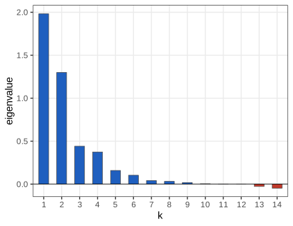
fig_9_8. Download: PDF · SVG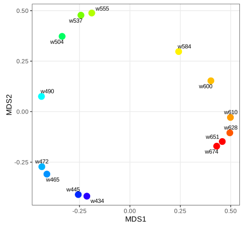
fig_9_9. Download: PDF · SVG9.2.2 Robust versions of MDS
Section 9.2.2 Result 9.3 shows that classical MDS fits squared inner products by least squares, so a single object far from all the others can dominate the map. A robust alternative keeps only the ranks of the dissimilarities.
Definition 9.2 (breakdown point) Section 9.2.2, margin note
The (finite-sample) breakdown point of an estimator \(T\) at a sample of size \(n\) is the smallest fraction \(m/n\) of observations that, replaced by arbitrary values, can carry \(T\) arbitrarily far.
Filling the gap 9.4: the mean breaks down at \(1/n\), the median at about \(1/2\) Section 9.2.2
Proof
Mean. Replace one observation \(x_1\) by \(x_1+c\); the mean moves by \(c/n\), unbounded in \(c\). So one point suffices: breakdown point \(1/n\).
Median. Let \(x_{(1)}\le\dots\le x_{(n)}\) be the original sample and replace \(m<n/2\) of the observations arbitrarily. At least \(n-m>n/2\) original values remain. The sample median is a value with at least half of the sample on each side; since more than half of the values are original, the median lies between the smallest and largest of the remaining original values, hence in \([x_{(1)},x_{(n)}]\), a bounded interval. With \(m=\lceil n/2\rceil\) replacements sent to \(+\infty\), the median follows them. The breakdown point is therefore \(\lceil n/2\rceil/n\to1/2\). ∎
(The book's sentence "even if we change 20 the numbers" should read "even if we change up to half of the numbers".) Rank-based procedures inherit this robustness: the rank of an observation is bounded no matter how extreme its value.
Nonmetric MDS (NMDS; Kruskal 1964) looks for a configuration \(\mathbf{X}\) in \(k\) dimensions, with distances \(d_{ij}=d_{ij}(\mathbf{X})\), and a non-decreasing function \(f\) such that the disparities \(\hat d_{ij}=f(\delta_{ij})\) of the input dissimilarities \(\delta_{ij}\) are close to the map distances.
Definition 9.3 (Kruskal's stress) Section 9.2.2
\[ \text{stress}(\mathbf{X})=\min_{f\ \text{non-decreasing}}\sqrt{\frac{\sum_{i<j}\big(d_{ij}(\mathbf{X})-f(\delta_{ij})\big)^2}{\sum_{i<j}d_{ij}(\mathbf{X})^2}}\,. \]This is "stress-1"; it is what vegan::metaMDS reports (checked to \(10^{-10}\)). It is invariant under rescaling of the map and depends on the \(\delta_{ij}\) only through their order.
The denominator of the stress Section 9.2.2, stress formula
The book writes \(\text{stress}^2\)
Filling the gap 9.5: how NMDS is computed (monotone regression and the Guttman transform) Section 9.2.2
The book calls metaMDS as a black box. The standard algorithm alternates two steps, each of which provably does not increase its objective.
Derivation
Step 1: optimal disparities for a fixed map (monotone regression). Order the pairs by \(\delta_{ij}\) (pairs with tied \(\delta\) are ordered by their current \(d_{ij}\), Kruskal's "primary approach"). The denominator of the stress does not involve \(f\), so we minimise \(\sum(d_{ij}-\hat d_{ij})^2\) over vectors \(\hat d\) that are non-decreasing in that order. The set of such vectors is a closed convex cone \(\mathcal{K}\), so the minimiser is the Euclidean projection of \(d\) onto \(\mathcal{K}\), which exists and is unique. The pool-adjacent-violators algorithm computes it: scan the sequence; whenever a value is smaller than the block before it, merge the two blocks and replace both by their (weighted) mean; repeat until the sequence is non-decreasing. (Optimality: at the solution, each block value is the mean of its \(d\)'s, and the KKT conditions of the projection hold because merging only occurs across violated constraints. Our implementation agrees with stats::isoreg.)
Step 2: a better map for fixed disparities (majorization). Rescale \(\hat d\) to have the same sum of squares as \(d\), and consider the raw stress \(\sigma(\mathbf{X})\)
with equality at \(\mathbf{X}=\mathbf{Z}\). So \(\sigma(\mathbf{X})\)
The sandwich \(\sigma(\mathbf{X}^+)\)metaMDS finds from 20 random starts. Because the stress has local minima, metaMDS restarts from random configurations; that randomness is why the book repeats it 100 times per dimension in Figure 9.10.
Algorithm 9.2 (nonmetric MDS by monotone regression and Guttman transforms) Section 9.2.2
- Start from a configuration \(\mathbf{X}\) in \(k\) dimensions (classical MDS, or random).
- Compute the map distances \(d_{ij}\) and the disparities \(\hat d\) by monotone regression of \(d\) on the order of \(\delta\); record the stress.
- Rescale \(\hat d\) to the size of \(d\) and update \(\mathbf{X}\leftarrow\frac1n\mathbf{B}(\mathbf{X})\mathbf{X}\).
- Repeat 2 and 3 until the stress stops decreasing; restart from several configurations and keep the best.
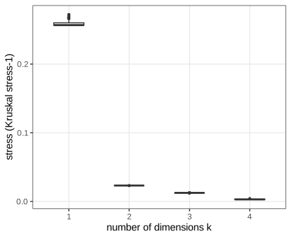
metaMDS reaches the same optimum almost every time on these 14 points. Reproduces Holmes and Huber (2019), Figure 9.10. Code: ch09_heterogeneous_data_a.R, fig_9_10. Download: PDF · SVGThe Shepard plot (Figure 9.11) draws the map distances against the input dissimilarities, with the fitted monotone step function \(f\). Its "non-metric fit" \(R^2=1-\text{stress}^2=0.999\) and the "linear fit" \(R^2\) (squared correlation of map distances and dissimilarities) are both high.
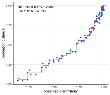
fig_9_11. Download: PDF · SVGFor these data the classical and nonmetric maps are almost identical (Figure 9.12): the dissimilarities are already close to Euclidean distances in the plane, up to a monotone transformation.
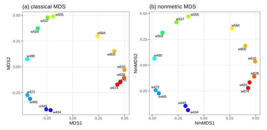
fig_9_12. Download: PDF · SVG9.3 Contiguous or supplementary information
Section 9.3 Covariates such as batch, date, protocol, treatment or clinical history are often filed as "metadata", as if they were less important than the assay. The book's point is the opposite: they are data, they must stay attached to the samples they describe, and they enter the multivariate analysis, typically as supplementary information that is projected onto a map without influencing it.
9.3.1 Known batches in data
Section 9.3.1 The example is Phylochip data (Holmes et al. 2011): normalised abundances of 8,634 bacterial taxa in 28 rat samples, from a study of healthy rats and rats with irritable bowel syndrome. The last row of the matrix is not a taxon but the day of hybridisation (1, 2 or 3), stored as a number: an awkward way of keeping a factor with an assay (Question 9.5). Instead of the abundances the analysis uses their ranks, a robust choice (Section 9.2.2): within each sample the taxa are ranked, all low ranks are tied at a threshold (the many taxa at noise level should not produce large rank jumps, Question 9.6), and a PCA (centred and scaled) is run on the 28 samples.
What the rank threshold does Section 9.3.1, function rankthreshPCA
The text says the transformation gives "the top 3000 most abundant taxa scores from 3000 to 1" and ties the rest. The code does something else: ranks run from 1 (least abundant) to 8,634, every rank below 3,000 is set to 3,000, and the score is \(3000-\text{rank}\). So the 2,999 least abundant taxa are tied at 0 and the 5,635 most abundant keep distinct (negative) scores (checked: 5,635 distinct ranks in every sample). Since PCA centres the columns, the sign is irrelevant; the substance is that "noise-level" is defined as the bottom 2,999 taxa, not everything outside the top 3,000. We reproduce the code.
With days 1 and 2 only, the screeplot (Figure 9.13) suggests two dimensions, and the samples fall into two groups, exactly the two days (Figure 9.14).
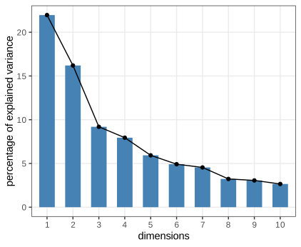
fig_9_13. Download: PDF · SVG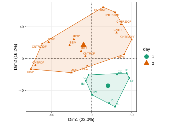
fig_9_14. Download: PDF · SVGOn day 1 and day 2 both the protocol and the array batch differed, so the two effects were confounded. A third batch of four samples (day 3) combined the day 2 arrays with the day 1 protocol; in the joint analysis it overlaps with day 1 (Figure 9.15), pointing at the protocol. The screeplot is nearly unchanged (Figure 9.16).
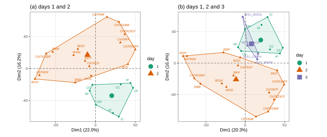
fig_9_15. Download: PDF · SVG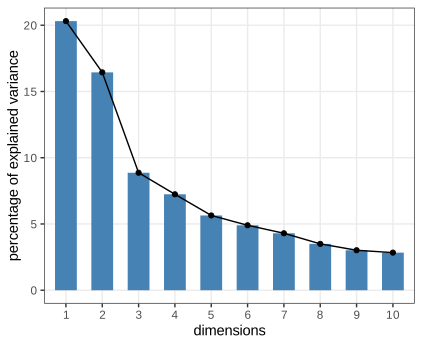
fig_9_16. Download: PDF · SVGFilling the gap 9.6: supplementary points and group barycentres Section 9.3.2 and footnote 6
The book calls the group means "supplementary points" without defining the projection. Here it is, with the property that justifies drawing them.
Derivation
Let \(\mathbf{Z}\) be the \(n\times p\) table used by the PCA (columns centred and scaled with the means and standard deviations of the active samples), with weights \(1/n\) on the rows. The principal axes are the unit eigenvectors \(\mathbf{v}_k\) of \(\frac1n\mathbf{Z}^\T\mathbf{Z}\), and the score of sample \(i\) on axis \(k\) is \(f_{ik}=\mathbf{z}_i^\T\mathbf{v}_k\). A supplementary row \(\mathbf{x}_s\), transformed with the same means and standard deviations into \(\mathbf{z}_s\), is placed at \(f_{sk}=\mathbf{z}_s^\T\mathbf{v}_k\); it plays no part in computing \(\mathbf{v}_k\), so the map is the same with or without it.
For a group \(G\) of active samples (a day, a treatment), the projection of its mean row is the mean of its projections, by linearity:
\[ \Big(\frac1{|G|}\sum_{i\in G}\mathbf{z}_i\Big)^\T\mathbf{v}_k=\frac1{|G|}\sum_{i\in G}f_{ik}. \]So the large symbols of Figures 9.14 and 9.15 are both "the group mean projected as a supplementary individual" and "the barycentre of the group on the map" (checked to \(10^{-13}\)). This is how a categorical variable enters a PCA as supplementary information: each of its levels becomes a barycentre. A level whose barycentre is far from the origin, compared with the spread of its points divided by \(\sqrt{|G|}\), is associated with the axes.
Question 9.7 (confidence ellipses around the group means)
When would ellipses around the group means (fviz_pca_ind(..., addEllipses = TRUE, ellipse.level = 0.69)) be preferable to convex hulls?
Answer
Hulls describe the spread of the individual samples and are driven by the most extreme ones. If the question is whether the batches differ in location, the relevant quantity is the uncertainty of each group mean, whose covariance is \(\bm\Sigma_G/|G|\) under independent sampling; an ellipse at a chosen level for a bivariate normal approximation of the group's coordinates then gives a visual test of separation. That is preferable with larger groups, when hulls overlap because of a few outlying samples even though the centres are clearly apart, and when groups have very different sizes (a hull of 4 points and a hull of 16 points are not comparable).
9.3.2 Removing batch effects
Section 9.3.2 Once a batch effect is known, the simplest correction subtracts each batch's mean from every feature, which moves all batch barycentres to the origin. ComBat (Johnson, Li and Rabinovic 2007; recommended by Leek et al. 2010) does this with an empirical Bayes model that also equalises variances and borrows strength across features. After ComBat the three days overlap (Figure 9.17).
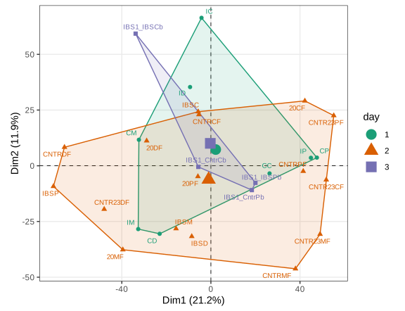
fig_9_17. Download: PDF · SVGFilling the gap 9.7: the location and scale model behind ComBat Section 9.3.2
The book describes ComBat as "a similar but slightly more sophisticated method (empirical Bayes)". Here is the model and the estimators.
Derivation
Model. For feature \(g\), batch \(i\) and sample \(j\) in that batch,
\[ Y_{gij}=\alpha_g+\mathbf{x}_{ij}^\T\bm\beta_g+\gamma_{gi}+\delta_{gi}\,\varepsilon_{gij},\qquad \varepsilon_{gij}\sim N(0,\sigma_g^2), \]with an additive batch effect \(\gamma_{gi}\) and a multiplicative one \(\delta_{gi}\), and covariates \(\mathbf{x}_{ij}\) whose effects must be protected (the book uses mod = ~1, i.e. none). After estimating \(\alpha_g,\bm\beta_g,\sigma_g\) by least squares (with the constraint \(\sum_i n_i\gamma_{gi}=0\)), standardise: \(Z_{gij}\)
Simple correction. Without priors, the maximum likelihood estimates are \(\hat\gamma_{gi}=\bar Z_{gi\cdot}\) and \(\hat\delta^2_{gi}\)
Empirical Bayes. ComBat puts priors across features, \(\gamma_{gi}\sim N(\gamma_i,\tau_i^2)\) and \(\delta^2_{gi}\sim\text{Inv-Gamma}(\lambda_i,\theta_i)\), with hyperparameters estimated by the method of moments from the \(\hat\gamma_{gi}\) and \(\hat\delta^2_{gi}\) of all features. Normal-normal conjugacy gives, conditional on \(\delta^2_{gi}\), a normal posterior for \(\gamma_{gi}\) with precision \(n_i/\delta^2_{gi}+1/\tau_i^2\) and mean
\[ \gamma^*_{gi}=\frac{n_i\tau_i^2\,\hat\gamma_{gi}+\delta^2_{gi}\,\gamma_i}{n_i\tau_i^2+\delta^2_{gi}}, \]a weighted average that shrinks the batch mean of feature \(g\) towards the mean over features, the more so the smaller \(n_i\). Conditional on \(\gamma_{gi}\), the inverse-gamma prior and the normal likelihood give the posterior
\[ \delta^2_{gi}\given\gamma_{gi},\text{data}\ \sim\ \text{Inv-Gamma}\Big(\lambda_i+\tfrac{n_i}2,\ \theta_i+\tfrac12\sum_j(Z_{gij}-\gamma_{gi})^2\Big), \]with mean
\[ \delta^{2*}_{gi}=\frac{\theta_i+\tfrac12\sum_j(Z_{gij}-\gamma^*_{gi})^2}{\tfrac{n_i}2+\lambda_i-1}. \]The two equations are iterated to a fixed point, and the adjusted data are \(Y^*_{gij}\)
Caution. The adjustment removes whatever is associated with batch. If the biology of interest is unbalanced across batches and not included in \(\mathbf{x}_{ij}\), part of it is removed too; here treatment was balanced within days, which is what makes the correction safe.
9.3.3 Hybrid data and Bioconductor containers
Section 9.3.3 A SummarizedExperiment stores one or more assays (features in rows, samples in columns) together with a colData table of sample covariates and a rowData table of feature annotations, kept aligned under subsetting. For the Phylochip data, SummarizedExperiment(assays = list(abundance = assayIBD), colData = DataFrame(day, treatment)) does it, and chipse[, day == 2] selects the 16 day-2 samples with their covariates (Question 9.8).
The second example is single-cell RNA-seq data from the workflow of Perraudeau et al. (2017): 1,000 highly variable genes in 747 cells from 18 batches (Question 9.9: length(unique(colData(corese)$Batch)) is 18), already normalised to remove batch effects. A PCA of the normalised values (Figure 9.18) suggests that axes 2 and 3 should be looked at together, and three-dimensional views coloured by batch and by the published clusters (Figure 9.19) show cells organised by cluster, not by batch.
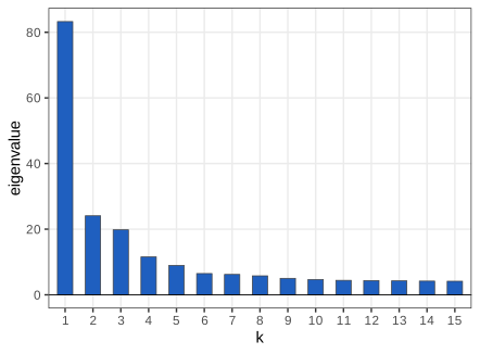
fig_9_18. Download: PDF · SVG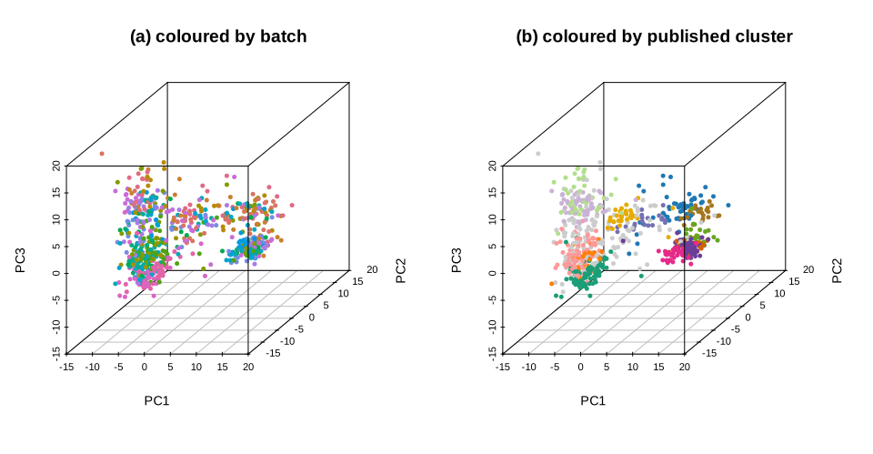
fig_9_19. Download: PDF · SVG9.4 Correspondence analysis for contingency tables
9.4.1 Cross-tabulation and contingency tables
Section 9.4.1 Two categorical variables measured on the same subjects give a contingency table of counts \(n_{ij}\). The rows and columns play symmetric roles: neither is "samples" nor "variables", so both are centred and both appear on the same map. The natural measure of structure is the departure from independence, measured by the chi-square statistic, which takes the place of the variance in PCA.
Data often arrive as a subject-by-category indicator matrix (Table 9.1 of the book: patients by HIV mutations, 0/1), which can be cross-tabulated into co-occurrence counts (Table 9.2: how many patients carry both mutations).
Question 9.10 (what cross-tabulation loses)
Answer
The co-occurrence matrix \(\mathbf{M}^\T\mathbf{M}\) of an indicator matrix \(\mathbf{M}\) keeps only pairwise counts. It loses which patient carries which mutations, all higher-order patterns (three mutations together; whether two pairs occur in the same patients or in different ones), and any patient-level covariates such as treatment history or time. It matters when mutations act in groups (resistance pathways need several mutations together), when patients are heterogeneous (pooling different treatment histories can create or hide associations, as in Simpson's paradox), and for inference: the pair counts of one patient are not independent observations.
Question 9.11 (testing independence of the mutations)
Answer
Mechanically, chisq.test on the 150 by 150 co-occurrence table gives \(X^2=724{,}268\) on 22,201 degrees of freedom, \(p<10^{-16}\). But the test is not valid here: its derivation (Filling the gap 9.10) assumes that every count is one independent observation classified by two factors, whereas a patient with \(m\) mutations contributes \(m(m-1)\) correlated pair counts, and the diagonal is structurally empty. A valid test of independence of two given mutations is a \(2\times2\) test on the patients (carrier of A or not, by carrier of B or not); for the whole table, a permutation test that shuffles each mutation's column of the patient-by-mutation matrix independently preserves the marginal frequencies and destroys association. Correspondence analysis remains a useful descriptive map either way.
The co-occurrence table of 150 mutations from the Stanford HIV drug resistance database (Rhee et al. 2003) is analysed with ade4::dudi.coa. Three eigenvalues stand out (Figure 9.20, 20.2%, 12.2% and 8.5% of the inertia), and the three-dimensional cloud (Figure 9.21) and its two planar views (Figure 9.22) show a few mutations far from the rest.
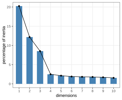
fig_9_20. Download: PDF · SVG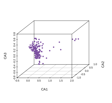
fig_9_21. Download: PDF · SVGQuestions 9.12 and 9.13 (the cloud in three dimensions; respecting the aspect ratio)
Answer
Rotating the cloud of Figure 9.21 (with rgl::plot3d, or car::scatter3d) shows a dense core and a few arms. With aspect = FALSE each axis is stretched to the same length, which exaggerates the third axis; equal scaling keeps distances interpretable. The points farthest out along the first axis are 116Y, 77L, 75I, 151M and 62V, the mutations of the multinucleoside-resistance complex around Q151M in reverse transcriptase, together with 65R further in: the first axis isolates a group of mutations that occur together. For the plane of axes 1 and 3 with the right proportions use coord_fixed() without setting different limits on the two axes, as in Figure 9.22(b).
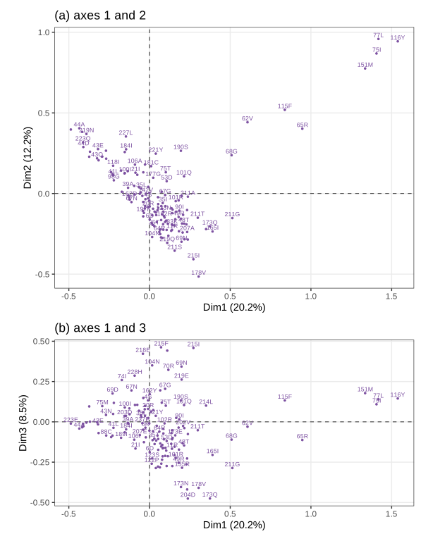
fig_9_22. Download: PDF · SVGThis first example maps the levels of one categorical variable (the mutations), much as PCA maps variables. The next example has two different variables.
9.4.2 Hair color, eye color and phenotype co-occurrence
Section 9.4.2 The data (R's HairEyeColor, female students) are a \(4\times4\) table of hair colour by eye colour; the chi-square test gives \(X^2=106.66\) on 9 degrees of freedom. The question is where the dependence lies. The residuals \(n_{ij}-e_{ij}\) from the table \(e_{ij}=n_{i\cdot}n_{\cdot j}/n\) expected under independence, scaled by \(\sqrt{e_{ij}}\), are coloured in the mosaic plot of Figure 9.23: blue-eyed blondes are far more frequent than independence predicts, brown-eyed blondes far less.
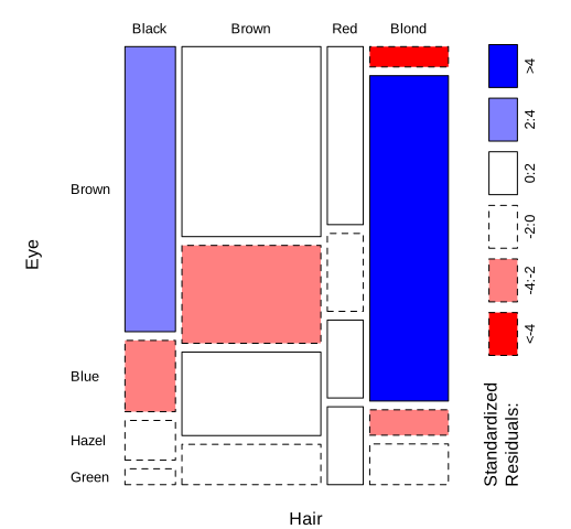
fig_9_23. Download: PDF · SVGDefinition 9.4 (masses, profiles, chi-square distance, inertia) Section 9.4.2, "Mathematical formulation"
Let \(\mathbf{N}\) be an \(I\times J\) table with total \(n\) and \(\mathbf{P}=\mathbf{N}/n\) (entries \(p_{ij}\)). The row and column masses are \(\mathbf{r}=\mathbf{P}\one\) and \(\mathbf{c}=\mathbf{P}^\T\one\), and \(\mathbf{D}_r=\diag(\mathbf{r})\), \(\mathbf{D}_c=\diag(\mathbf{c})\). The profile of row \(i\) is \(\mathbf{a}_i=(p_{i1},\dots,p_{iJ})/r_i\), a probability vector; the average row profile is \(\sum_ir_i\mathbf{a}_i=\mathbf{c}\). The chi-square distance between two row profiles is \(d^2_{\chi}(\mathbf{a},\mathbf{a}')\)
A notational slip Section 9.4.2, display after "can also be written"
The book writes "\(\mathbf{N}\)
Result 9.4 (CA decomposes the chi-square statistic) Section 9.4.2; Question 9.14
Let \(\mathbf{S}\)
and \(\rank\mathbf{S}\le\min(I,J)-1\). The eigenvalues of CA are \(\lambda_k=\gamma_k^2\); the first \(K\) axes "explain" the fraction \(\sum_{k\le K}\lambda_k/\sum_k\lambda_k\) of the chi-square statistic.
Filling the gap 9.8: correspondence analysis is an SVD of standardised residuals Section 9.4.2 ("a special weighted version of SVD")
Derivation
Chi-square and inertia. With \(p_{ij}=n_{ij}/n\) and \(e_{ij}=nr_ic_j\),
\[ \frac{(n_{ij}-e_{ij})^2}{n\,e_{ij}}=\frac{n^2(p_{ij}-r_ic_j)^2}{n^2r_ic_j}=\frac{(p_{ij}-r_ic_j)^2}{r_ic_j}=s_{ij}^2, \]so \(X^2/n\)
Rank. \(\mathbf{S}\,\mathbf{D}_c^{1/2}\one\)
Coordinates. The principal coordinates of the rows and columns are \(\mathbf{F}\)$li and $co); the standard coordinates omit \(\bm\Gamma\). Three properties make the map interpretable:
- Each axis is centred and has weighted variance \(\lambda_k\): \(\sum_ir_if_{ik}\)
\({}=\sqrt{\mathbf{r}}^\T\mathbf{u}_k\gamma_k\) \({}=0\) and \(\sum_ir_if_{ik}^2\) \({}=\gamma_k^2\,\mathbf{u}_k^\T\mathbf{u}_k\) \({}=\lambda_k\). - Euclidean distances between rows of \(\mathbf{F}\) (all axes) are chi-square distances between profiles: \(\mathbf{F}\mathbf{F}^\T\)
\({}=\mathbf{D}_r^{-1/2}\mathbf{S}\mathbf{S}^\T\mathbf{D}_r^{-1/2}\) \({}=(\mathbf{A}-\one\mathbf{c}^\T)\mathbf{D}_c^{-1}(\mathbf{A}-\one\mathbf{c}^\T)^\T\), with \(\mathbf{A}=\mathbf{D}_r^{-1}\mathbf{P}\) the matrix of profiles. So CA is a weighted PCA of the profiles in the chi-square metric, and also a weighted MDS of the chi-square distances. - Distributional equivalence: if two columns have proportional entries, merging them changes neither the chi-square distances between rows nor the eigenvalues (the term \((a_{j}-a'_{j})^2/c_j\) splits proportionally). Category definitions that only split or merge equivalent categories do not change the analysis (checked on the hair and eye table).
Our SVD gives ade4's eigenvalues and coordinates to machine precision, and \(X^2/n\) equals the total inertia for the hair and eye data (\(106.66/313=0.341\)).
Result 9.5 (barycentric or transition formulas) Section 9.4.2, "Interpreting the biplots"
With \(\bm\Phi=\mathbf{D}_r^{-1/2}\mathbf{U}\) and \(\bm\Psi=\mathbf{D}_c^{-1/2}\mathbf{V}\) the standard coordinates,
\[ \mathbf{F}=\mathbf{D}_r^{-1}\mathbf{P}\,\bm\Psi,\qquad \mathbf{G}=\mathbf{D}_c^{-1}\mathbf{P}^\T\bm\Phi: \]each row point in principal coordinates is the average of the column points in standard coordinates, weighted by the row's profile; and symmetrically for columns.
Filling the gap 9.9: proof of the barycentric property, and which biplot it holds in Section 9.4.2
Proof
From \(\mathbf{S}\mathbf{V}\)
Which map. The book says that the biplot scaling places the row points at the centres of gravity of the column levels. This is exact in the asymmetric map (rows in principal, columns in standard coordinates). The default fviz_ca_biplot of Figure 9.24 is the symmetric map, both sets in principal coordinates, \(\mathbf{G}=\bm\Psi\bm\Gamma\); there the row point is the barycentre of the column points only after stretching axis \(k\) by \(1/\gamma_k\) (for the hair data \(\gamma_1=0.55\), so the stretch is almost a factor 2). In the symmetric map, closeness of a row and a column point is suggestive but not a distance; what is exact is the distances among rows, and among columns, as chi-square distances.
For the hair and eye table the first axis carries 88.8% of the inertia and the second 9.6% (book: 89, 10, 2), so the plane shows 98.3% of the chi-square (Question 9.14). The first axis opposes blond hair and blue eyes to black or brown hair and brown eyes (Figure 9.24).
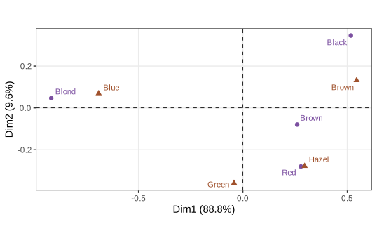
fig_9_24. Download: PDF · SVGQuestion 9.15 (vegan's cca with the right scaling)
Answer
vegan::cca(HairColor) without constraints is the same correspondence analysis (same eigenvalues). Its plot method offers scaling 1 (rows in principal, columns in standard coordinates: row-to-row distances are chi-square distances and rows are barycentres of columns), scaling 2 (the reverse) and scaling 3, "symmetric", where both are multiplied by \(\sqrt{\gamma_k}\). Scaling 3 is the closest analogue of the symmetric map of Figure 9.24; the two differ only by a factor \(\sqrt{\gamma_k}\) per axis, and by vegan's convention of scaling the scores with a constant that depends on the table total.
Filling the gap 9.10: why \(X^2\) has \((I-1)(J-1)\) degrees of freedom Section 9.4.2 (the chi-square test of Chapter 2)
Derivation (sketch with the key steps)
Assume \(n\) independent subjects, each falling in cell \((i,j)\) with probability \(\pi_{ij}\), and independence \(\pi_{ij}=\rho_i\kappa_j\). By the multivariate central limit theorem the vector \(\mathbf{w}\) with entries \(w_{ij}\)
Filling the gap 9.11: the duality diagram \((\mathbf{X},\mathbf{Q},\mathbf{D})\) Section 9.6.4, "see Holmes (2006)"; ade4's dudi objects
PCA, CA and MDS look different, but ade4 (whose dudi.* functions the book uses throughout) treats them as one analysis of a triplet. This is the French "duality diagram" (Escoufier 1987; Holmes 2006).
Derivation
A triplet is a data matrix \(\mathbf{X}\) (\(n\times p\)), a symmetric positive definite \(p\times p\) metric \(\mathbf{Q}\) on the variables (it defines distances between rows: \(\|\mathbf{x}_i-\mathbf{x}_{i'}\|_\mathbf{Q}^2\)
- PCA: \(\mathbf{X}\) centred (and scaled), \(\mathbf{Q}=\mathbf{I}\), \(\mathbf{D}=\frac1n\mathbf{I}\). Then \(\mathbf{X}^\T\mathbf{D}\mathbf{X}\) is the covariance (correlation) matrix.
- CA: \(\mathbf{X}\)
\({}=\mathbf{D}_r^{-1}\mathbf{P}\mathbf{D}_c^{-1}-\one\one^\T\), \(\mathbf{Q}=\mathbf{D}_c\), \(\mathbf{D}=\mathbf{D}_r\). Then \(\widetilde{\mathbf{X}}\) \({}=\mathbf{D}_r^{1/2}\mathbf{X}\mathbf{D}_c^{1/2}\) \({}=\mathbf{D}_r^{-1/2}\mathbf{P}\mathbf{D}_c^{-1/2}-\sqrt{\mathbf{r}}\sqrt{\mathbf{c}}^\T\) \({}=\mathbf{S}\), the matrix of Result 9.4. The metric \(\mathbf{Q}=\mathbf{D}_c\) applied to \(x_{ij}=a_{ij}/c_j-1\) is exactly the chi-square distance between profiles. - MDS: the row analysis \(\mathbf{X}\mathbf{Q}\mathbf{X}^\T\mathbf{D}\) with \(\mathbf{D}=\mathbf{I}\) only needs the inner-product matrix \(\mathbf{W}\)
\({}=\mathbf{X}\mathbf{Q}\mathbf{X}^\T\), which is \(\mathbf{B}\) of (9.1): MDS is the case where \(\mathbf{W}\) is given (through distances) and \(\mathbf{X}\) is not.
We compute the CA eigenvalues of the hair and eye table and the PCA eigenvalues of the iris data from the triplet formula and compare them with dudi.coa and dudi.pca. Multitable methods (RV, co-inertia, CCA, Section 9.6) compare the matrices \(\mathbf{W}\)
9.5 Finding time and other important gradients
Section 9.5 Clustering looks for a hidden categorical variable; ordination looks for a hidden ordering: time, an environmental gradient, a developmental path. Ecologists long ago noticed that a gradient shows up in CA and PCA maps as an arch (or horseshoe), and archaeologists used the same idea to date objects by seriation (Kendall 1969). The book's toy example is a table of 15 plant species counted at 10 locations along a lakeshore. CA puts 56% of the inertia on the first axis and 25% on the second, and the locations lie on an arch in their spatial order (Figure 9.25).
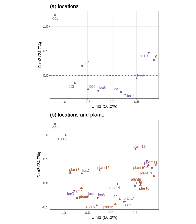
fig_9_25. Download: PDF · SVGQuestion 9.16 (the pattern in the raw table)
Answer
The table is nearly a band matrix: plant 1 is abundant at location 1, plant 2 at locations 1 to 3, and so on, so the large counts run down the diagonal. Each species has a unimodal response along the gradient, with optima in the same order as the locations. Had the plants been listed in alphabetical order of their names, the band would be invisible in the printed table, but CA would give exactly the same map: CA is invariant under permutations of rows and columns. Recovering the hidden order is precisely what the arch does (seriation).
Result 9.6 (why a gradient produces an arch) Section 9.5; Diaconis, Goel and Holmes (2008)
Let objects sit at positions \(t_1<\dots<t_n\) along a gradient and let their similarity decrease with \(|t_i-t_j|\) (or their dissimilarity saturate: objects far apart share nothing, whatever the distance). Then the leading eigenvectors of the centred similarity matrix are close to the cosines \(\cos(\pi t)\), \(\cos(2\pi t)\), \(\dots\) (with \(t\) rescaled to \((0,1)\)), and because \(\cos(2u)=2\cos^2u-1\) the points \((\text{axis 1},\text{axis 2})\) lie close to a parabola: an arch whose second coordinate is a function of the first, not a second latent variable.
Filling the gap 9.12: the mathematics of the horseshoe Section 9.5
The book mentions the arch and cites Diaconis, Goel and Holmes (2008). Here is a self-contained argument: an exact statement for the simplest operator, and a controlled approximation for a standard similarity.
Derivation
(a) The path graph. Link consecutive objects on the gradient and let \(\mathbf{L}\) be the Laplacian of the path: \(L_{ii}\) is the number of neighbours (1 at the ends, 2 inside), \(L_{i,i\pm1}=-1\). For \(k=0,\dots,n-1\) let \(\theta=\pi k/n\) and \(v_k(i)=\cos\big(\theta(i-\tfrac12)\big)\). For an interior row, \(\cos(x-\theta)+\cos(x+\theta)\)
(b) A similarity that decays along the gradient. Take \(K_{ij}=\rho^{|i-j|}\) with \(0<\rho<1\) (the Kac-Murdock-Szegő matrix; similarity decays exponentially with separation). Its inverse is tridiagonal: one checks directly that
\[ (1-\rho^2)\,\mathbf{K}^{-1}=(1+\rho^2)\mathbf{I}-\rho\mathbf{A}-\rho^2(\mathbf{e}_1\mathbf{e}_1^\T+\mathbf{e}_n\mathbf{e}_n^\T)=\rho\,\mathbf{L}+(1-\rho)^2\mathbf{I}+\rho(1-\rho)(\mathbf{e}_1\mathbf{e}_1^\T+\mathbf{e}_n\mathbf{e}_n^\T), \]with \(\mathbf{A}\) the adjacency matrix of the path. The identity term does not change eigenvectors, so up to a perturbation of the two corner entries, \(\mathbf{K}^{-1}\) is an increasing function of \(\mathbf{L}\), and the largest eigenvectors of \(\mathbf{K}\) are close to the discrete cosines. The approximation is good when the similarity decays slowly (\(\rho\) near 1): with \(n=60\), \(\rho=0.98\), the first two eigenvectors of the centred matrix \(\mathbf{H}\mathbf{K}\mathbf{H}\) correlate above 0.99 with \(\cos(\pi t)\) and \(\cos(2\pi t)\), and a quadratic in axis 1 explains more than 95% of axis 2 (checked).
(c) The arch. If axis 1 is \(x_i=a\cos(\pi t_i)\) and axis 2 is \(y_i=b\cos(2\pi t_i)\), then \(y_i=b\,(2x_i^2/a^2-1)\): the points lie exactly on a parabola. When the similarity decays fast (a kernel with small \(\rho\), or a PCA of species with narrow niches), higher cosines mix in, the ends of the arch curl inwards and the shape becomes a true horseshoe; points far apart on the gradient can then be close on the map.
Consequences. (i) The second axis of an arch is not a second biological factor; it is the square of the first. (ii) The ordering along the gradient is recovered by the position along the arch (approximately the order on axis 1, or the angle around the horseshoe), which is seriation. (iii) Kernel and MDS methods with saturating dissimilarities show the same effect (Ekman's colours, Figure 9.9). For the lake data, a quadratic in CA axis 1 explains 88% of the variance of axis 2.
9.5.1 Dynamics of cell development
Section 9.5.1 Moignard et al. (2015) measured the expression of 46 genes by single-cell qPCR in 3,934 mouse embryo cells from five populations between embryonic days 7.0 and 8.25: primitive streak (PS), neural plate (NP), head fold (HF), and two populations at the four-somite stage, 4SG and 4SFG\(^-\) (the book's Figure 9.26 is a schematic of these stages and is not reproduced). Classical MDS on the \(\ell_1\) (Manhattan) and \(L_2\) (Euclidean) distances between cells gives two dominant eigenvalues in both cases (Figure 9.27); the first two axes carry 78% (\(\ell_1\)) and 57% (\(L_2\)) of the sum of all eigenvalues.
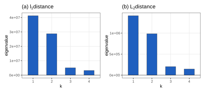
fig_9_27. Download: PDF · SVGRemark: the \(\ell_1\) percentage Section 9.5.1
The \(L_2\) distances between cells are Euclidean, so all eigenvalues of \(\mathbf{B}\) are non-negative and 57% is a fraction of a total variance. The \(\ell_1\) distances are not Euclidean: 3,309 of the 3,934 eigenvalues are negative, the smallest being \(-6.8\%\) of the largest. Their sum reduces \(\Tr\mathbf{B}\), so "78%" is the first two eigenvalues divided by a total that has had the negative part subtracted; the two percentages are not comparable. (The square root of an \(\ell_1\) distance is Euclidean, so MDS on \(\sqrt{d_{\ell_1}}\) would avoid the problem.)
Both first planes show the same organisation (Figure 9.28): a continuous path from the PS cells (blue) through NP and HF to the four-somite cells, with the 4SG cells (red) forming a separate, elongated cluster.
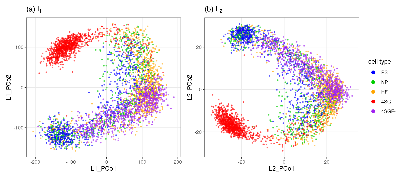
fig_9_28. Download: PDF · PNG9.5.2 Local, nonlinear methods
Section 9.5.2 MDS tries to represent all distances, and the large ones dominate. When the data lie near a curved low-dimensional set (a trajectory), only small distances are reliable measures of how close two cells are along the trajectory; large distances cut across the curve. Local methods therefore down-weight large distances, for instance through a kernel.
Question 9.17 (the radial basis kernel)
Why use \(1-\exp(-d(x,y)^2/\sigma^2)\), and what happens for large distances?
Answer
The kernel \(k=\exp(-d^2/\sigma^2)\) is a similarity (1 for identical points, decreasing to 0). Subtracting it from 1 turns it into a dissimilarity that is 0 at \(d=0\), increasing in \(d\), and bounded by 1. For \(d\ll\sigma\) a Taylor expansion gives \(1-k\approx d^2/\sigma^2\): small distances are kept (squared and rescaled). For \(d\gg\sigma\), \(1-k\approx1\): all large distances become nearly equal, so their exact values no longer influence the map. The bandwidth \(\sigma\) decides which distances count as "small".
Filling the gap 9.13: kernel MDS is kernel PCA, and what the book's \(\sigma\) does Section 9.5.2; Exercise 9.6
Derivation
Let \(k\) be a positive definite kernel with \(k(x,x)=1\) and feature map \(\varphi\), \(k(x,y)\)
because \(\mathbf{H}\one\one^\T\mathbf{H}\)
The book's code (Exercise 9.6) passes \(1-k\) to cmdscale as a distance, which squares it, so it analyses \((1-k)^2\) rather than \(2(1-k)\). And its bandwidths are tiny compared with the data: rbfdot(sigma = (1/3934)^2) is \(k=\exp(-\sigma d^2)\) with \(\sigma d^2<10^{-3}\) for all pairs of cells (checked), so \(1-k=\sigma d^2\) to four digits and the analysed "distance" is \(\sigma^2d^4\); 3,888 of its eigenvalues are negative. laplacedot(sigma = 1/3934) is \(\exp(-\sigma d)\) with \(\sigma d\le0.02\), so \(1-k\approx\sigma d\) and the result is plain MDS on Euclidean distances. Neither kernel discounts large distances at these settings. To obtain the intended local behaviour, \(\sigma\) must be comparable to the inverse of a typical squared distance (for the Gaussian kernel, \(1/\text{median}(d^2)\)), and the input to cmdscale should be \(\sqrt{2(1-k)}\).
t-SNE (van der Maaten and Hinton 2008) is the most widely used local method. On the cell data, a two-dimensional t-SNE separates the 4SG cells and the PS cells as tight groups, and the third axis of a three-dimensional t-SNE separates further structure (Figures 9.29 and 9.30).
Filling the gap 9.14: what t-SNE optimises, and its gradient Section 9.5.2
The book describes t-SNE as letting \(\sigma^2\) "vary locally (there is a normalization step so that it averages to one)". More precisely, each point gets its own bandwidth, chosen to fix the entropy of its neighbour distribution.
Derivation
High-dimensional similarities. For point \(i\) let
\[ p_{j\given i}=\frac{\exp(-\beta_i\|\mathbf{x}_i-\mathbf{x}_j\|^2)}{\sum_{k\ne i}\exp(-\beta_i\|\mathbf{x}_i-\mathbf{x}_k\|^2)}, \]with \(\beta_i=1/(2\sigma_i^2)\). The perplexity \(e^{H(P_i)}\), with \(H(P_i)\)
Dense regions get large \(\beta_i\) (small \(\sigma_i\)), sparse ones small \(\beta_i\). The joint similarities are \(p_{ij}\)
Low-dimensional similarities and objective. In the map, \(w_{ij}\)
Gradient. \(C\)
which agrees with finite differences. Pairs with \(p_{ij}>q_{ij}\) attract, the others repel. The heavy tail of the \(t_1\) kernel lets moderately distant points end up far apart without much cost, which is why t-SNE separates clusters so clearly, and also why distances between clusters, and cluster sizes, carry little information (the book's warning).
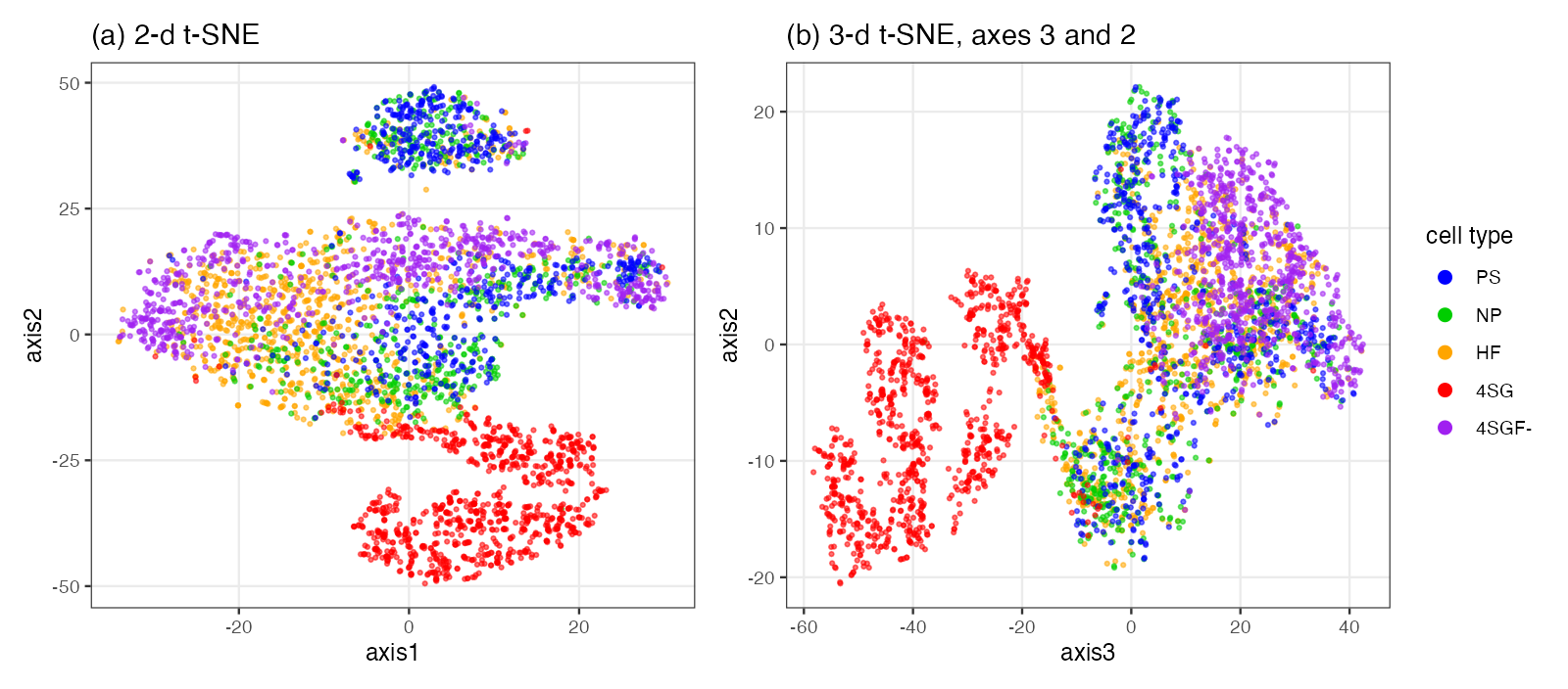
fig_9_29. Download: PDF · PNG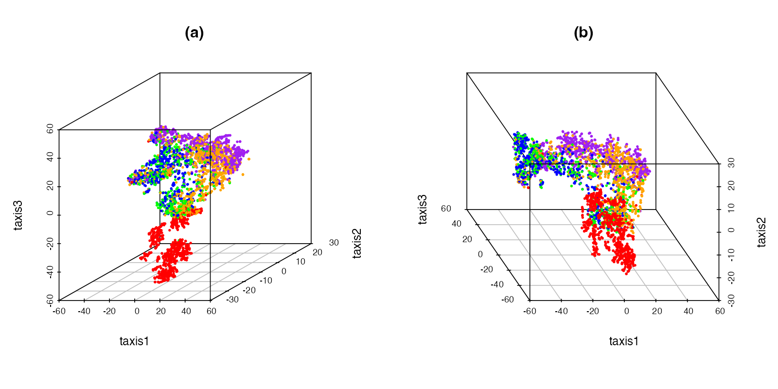
fig_9_30. Download: PDF · PNGQuestion 9.18 (t-SNE of the Ukraine distances)
Answer
Pass the distance matrix with is_distance = TRUE and a perplexity below \((n-1)/3=10.7\) (8 in the book); see Figure 9.31. The map keeps neighbourhoods (Lviv with Ternopil and Lutsk, Simferopol with Sevastopol) but distorts the global shape: it stretches the country, and distances between regions are not proportional to kilometres.
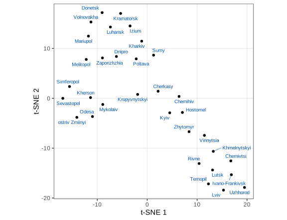
fig_9_31. Download: PDF · SVGOther nonlinear methods mentioned by the book: locally linear embedding and Isomap (RDRToolbox), diffusion maps (diffusionMap, used in Exercises 9.7 and 9.8), kernel methods (kernlab) and local principal curves (LPCM).
9.6 Multitable techniques
Section 9.6 Studies now often measure several kinds of features on the same samples: microbes, metabolites, genes. The first question is whether the tables carry related information at all, the second which features drive the relationship.
9.6.1 Co-variation, inertia, co-inertia and the RV coefficient
Section 9.6.1 Inertia is the weighted sum of squared distances of points to their centre of gravity: variance for a PCA, \(X^2/n\) for a CA (Result 9.4). For two variables measured at the same \(n\) sites, standardised, the covariation is \(\cov(x,y)=\frac1n\sum_ix_iy_i\) (the book's (9.2) writes the mean of the single sum \(x_1y_1+\dots+x_{10}y_{10}\); it means the mean of the ten products). Co-inertia generalises this to two tables: for configurations \(\mathbf{X}\) (\(n\times p\)) and \(\mathbf{Y}\) (\(n\times q\)) with centred columns, \(\Tr(\mathbf{X}^\T\mathbf{D}\mathbf{Y}\mathbf{Y}^\T\mathbf{D}\mathbf{X})\)
9.6.2 Mantel coefficient and a test of distance correlation
Section 9.6.2 Given two dissimilarity matrices \(\mathbf{D}^X,\mathbf{D}^Y\) on the same \(n\) objects, the Mantel coefficient is the Pearson correlation of their \(m=n(n-1)/2\) off-diagonal entries:
\[ r_m(\mathbf{X},\mathbf{Y})=\frac{\sum_{i<j}(d^X_{ij}-\bar d^X)(d^Y_{ij}-\bar d^Y)}{\sqrt{\sum_{i<j}(d^X_{ij}-\bar d^X)^2\,\sum_{i<j}(d^Y_{ij}-\bar d^Y)^2}}. \](The book sums over \(i\ne j\); since both matrices are symmetric this counts every pair twice and gives the same value.) Unlike the RV coefficient below, it involves no double centring.
Filling the gap 9.15: why the Mantel test permutes objects, and why its p-value is valid Section 9.6.2
Derivation
The \(m\) pairs are not independent observations: the \(n-1\) distances involving object \(i\) all share it, so the usual \(t\) test for a correlation, which assumes \(m\) independent pairs, is far too liberal. The null hypothesis is that the labelling of the objects in \(\mathbf{D}^Y\) is unrelated to that in \(\mathbf{D}^X\), formally that the joint distribution is invariant when the rows and columns of \(\mathbf{D}^Y\) are permuted together by any permutation \(\pi\) of the objects, \(d^Y_{ij}\mapsto d^Y_{\pi(i)\pi(j)}\) (true, for instance, if the objects are i.i.d. and the two measurements are independent). Under this exchangeability, the observed statistic \(r_0\) and the statistics \(r_1,\dots,r_B\) computed after \(B\) independent uniform random permutations are exchangeable, so the rank of \(r_0\) among the \(B+1\) values is uniform (ties only help). Therefore
\[ p=\frac{1+\#\{b\ge1:\ r_b\ge r_0\}}{B+1}\quad\text{satisfies}\quad P(p\le\alpha)\le\alpha\ \text{ for every }\alpha, \]a valid p-value for any \(B\) (vegan's mantel uses this formula, checked). The caution of Guillot and Rousset (2013) is about the null hypothesis: with spatially autocorrelated data, permuting sites destroys the autocorrelation, exchangeability fails, and the test rejects too often even when the two variables are unrelated.
9.6.3 The RV coefficient
Section 9.6.3 The RV coefficient (Escoufier 1973) compares two tables on the same \(n\) rows through their configuration matrices \(\mathbf{W}_X=\mathbf{X}\mathbf{X}^\T\) and \(\mathbf{W}_Y=\mathbf{Y}\mathbf{Y}^\T\) (centred columns, often scaled), the \(n\times n\) matrices of inner products between samples:
\[ \RV(\mathbf{X},\mathbf{Y})=\frac{\Tr(\mathbf{W}_X\mathbf{W}_Y)}{\sqrt{\Tr(\mathbf{W}_X^2)\,\Tr(\mathbf{W}_Y^2)}}=\frac{\|\mathbf{X}^\T\mathbf{Y}\|_F^2}{\|\mathbf{X}^\T\mathbf{X}\|_F\,\|\mathbf{Y}^\T\mathbf{Y}\|_F}. \]The book's RV formula Section 9.6.3
The book writes \(\RV(A,B)\)
Result 9.7 (properties of the RV coefficient) Section 9.6.3
(a) \(0\le\RV\le1\). (b) \(\RV=1\) if and only if \(\mathbf{W}_Y=c\,\mathbf{W}_X\) for some \(c>0\), i.e. the two configurations of samples agree up to rotation and global scaling (for instance \(\mathbf{Y}=c\,\mathbf{X}\mathbf{Q}\) with \(\mathbf{Q}\) orthogonal). (c) For \(p=q=1\), \(\RV=\cor(x,y)^2\). (d) Under random permutations of the rows of \(\mathbf{Y}\),
\[ \E_\pi[\RV]=\frac{\sqrt{\beta_X\beta_Y}}{n-1},\qquad \beta_X=\frac{(\Tr\mathbf{W}_X)^2}{\Tr(\mathbf{W}_X^2)}\in[1,\rank\mathbf{X}]. \]Filling the gap 9.16: proofs, and why 0.84 must be compared with 0.31 Section 9.6.3, RV.rtest output
Proof
(a) \(\Tr(\mathbf{W}_X\mathbf{W}_Y)\)
(d) Let \(\mathbf{P}_\pi\) be a uniformly random permutation matrix. The denominator is invariant. For the numerator, \(\E[(\mathbf{P}_\pi\mathbf{W}_Y\mathbf{P}_\pi^\T)_{ii}]\)
and dividing by the denominator gives the formula (Kazi-Aoual et al. 1995; Josse, Pagès and Husson 2008). We verify it exactly over all 720 permutations of a 6-row example. \(\beta_X\) is an effective rank: 1 if \(\mathbf{X}\) has rank one, \(\rank\mathbf{X}\) if all its singular values are equal.
Consequence. With few samples and many variables the RV coefficient of unrelated tables is far from 0. For the microbe and metabolite tables (\(n=12\)) the exact permutation mean is 0.314 (the book's RV.rtest prints a simulated "Expectation" of 0.318), so the observed 0.840 should be judged against 0.31, not against 0, which is what the permutation test does (p = 0.002 with 999 permutations). Adjusted versions subtract this expectation (Josse and Holmes 2016).
9.6.4 Canonical correlation analysis (CCA)
Section 9.6.4 Hotelling's canonical correlation analysis looks for a linear combination \(U=\mathbf{X}\mathbf{a}\) of the \(p\) columns of \(\mathbf{X}\) and one \(V=\mathbf{Y}\mathbf{b}\) of the \(q\) columns of \(\mathbf{Y}\) (both \(n\) rows; the book's "\(n\times p\) matrix \(Y\)" should read \(n\times q\), and the last term of \(V\) is \(b_qY_q\)) that are as correlated as possible:
\[ \rho_1=\max_{\mathbf{a},\mathbf{b}}\cor(\mathbf{X}\mathbf{a},\mathbf{Y}\mathbf{b})\quad\text{subject to}\quad\var(\mathbf{X}\mathbf{a})=\var(\mathbf{Y}\mathbf{b})=1, \tag{9.3} \]and then, for \(s=2,3,\dots\), \(\rho_s\)
Result 9.8 (CCA is a generalised eigenproblem, and an SVD) Section 9.6.4, (9.3) to (9.5)
Let \(\mathbf{S}_{xx},\mathbf{S}_{yy},\mathbf{S}_{xy}\) be the sample covariance matrices (\(\mathbf{S}_{xx},\mathbf{S}_{yy}\) invertible), and \(\mathbf{M}\)
The canonical variates satisfy (9.5) automatically, and moreover \(\cor(U^s,V^t)=0\) for \(s\ne t\).
Filling the gap 9.17: derivation of CCA Section 9.6.4 ("presented as a problem solved through an iterative algorithm")
Derivation
First pair. The correlation does not depend on the scale of \(\mathbf{a}\) or \(\mathbf{b}\), so (9.3) is: maximise \(\mathbf{a}^\T\mathbf{S}_{xy}\mathbf{b}\) subject to \(\mathbf{a}^\T\mathbf{S}_{xx}\mathbf{a}\)
stationarity gives \(\mathbf{S}_{xy}\mathbf{b}\)
As an SVD. Substitute \(\tilde{\mathbf{a}}\)
Later pairs. \(\cor(U^s,U^t)\)
Geometry. The \(\rho_k\) are the cosines of the principal angles between the column spaces of the centred \(\mathbf{X}\) and \(\mathbf{Y}\), so they are invariant under any invertible linear recoding of either table's variables. We compare both formulas with cancor to \(10^{-13}\) and confirm that the canonical variates are uncorrelated.
Result 9.9 (CCA overfits when \(p+q\ge n\)) Section 9.6.5 ("finding two very correlated vectors can be too easy")
Let \(\mathbf{X}\) and \(\mathbf{Y}\) have centred columns. If \(\dim\col(\mathbf{X})+\dim\col(\mathbf{Y})>n-1\), then \(\rho_1=1\), whatever the data. In particular, if \(\rank\mathbf{X}=n-1\) (generically, as soon as \(p\ge n-1\)), every linear combination of \(\mathbf{Y}\) is perfectly predicted by one of \(\mathbf{X}\).
Proof
Both column spaces lie in \(\one^\perp\), which has dimension \(n-1\). Two subspaces whose dimensions add to more than \(n-1\) intersect in a nonzero vector \(\mathbf{u}\)
The microbe and metabolite data have \(n=12\), \(p=174\) OTUs and \(q=405\) metabolites, so classical CCA returns \(\rho_1=1\) and is meaningless: against 3 metabolites, 9 OTUs already suffice, since \(9+3>11\) (checked). This is the reason for the sparse version.
9.6.5 Sparse canonical correlation analysis (sCCA)
Section 9.6.5 The data of Kashyap et al. (2013) are 12 mouse samples (knockout and wild type, two diets) with bacterial OTU abundances and metabolite abundances. After the book's filtering and \(\log_{10}(1+x)\) transformation there are 174 OTUs and 405 metabolites. The RV coefficient is 0.840 with permutation p-value 0.002. Sparse CCA with PMA::CCA(penaltyx = 0.15, penaltyz = 0.15) selects 5 OTUs and 16 metabolites whose combinations correlate at 0.990.
Filling the gap 9.18: the penalised matrix decomposition behind PMA::CCA Section 9.6.5
The book says a penalty "maintains the number of non-zero coefficients to a minimum" and leaves the method to the package. Here is what it solves (Witten, Tibshirani and Hastie 2009) and why the algorithm works.
Derivation
The problem. Standardise the columns of \(\mathbf{X}\) (\(n\times p\)) and \(\mathbf{Y}\) (\(n\times q\)). When \(p,q\gg n\), \(\mathbf{S}_{xx}\) and \(\mathbf{S}_{yy}\) are singular, and the sparse CCA of PMA ("standard" type) replaces them by identity matrices, adding \(\ell_1\) bounds:
\[ \max_{\mathbf{u},\mathbf{v}}\ \mathbf{u}^\T\mathbf{X}^\T\mathbf{Y}\mathbf{v}\quad\text{s.t.}\quad\|\mathbf{u}\|_2\le1,\ \|\mathbf{v}\|_2\le1,\ \|\mathbf{u}\|_1\le c_1,\ \|\mathbf{v}\|_1\le c_2 . \]For unit vectors \(1\le\|\mathbf{u}\|_1\le\sqrt p\), so \(c_1\in[1,\sqrt p]\); PMA's penaltyx is \(c_1/\sqrt p\) (0.15 gives \(c_1=0.15\sqrt{174}=1.98\), and \(c_2=0.15\sqrt{405}=3.02\)).
One block at a time. For fixed \(\mathbf{v}\), with \(\mathbf{g}\)
with \(\Delta=0\) if \(\|\mathbf{g}\|_1/\|\mathbf{g}\|_2\)
The algorithm. Start from the leading right singular vector of \(\mathbf{X}^\T\mathbf{Y}\) and alternate the two updates. Each update maximises the objective over one block with the other fixed, so the objective never decreases (up to the bisection tolerance), and it is bounded by \(\sigma_1(\mathbf{X}^\T\mathbf{Y})\); the iterates converge to a stationary point of this biconvex problem, not necessarily the global maximum. Our own implementation selects exactly the same 5 OTUs and 16 metabolites as PMA, with \(\cor(\mathbf{X}\mathbf{u},\mathbf{Y}\mathbf{v})\)
Cautions (some in the book). With 12 samples, a correlation of 0.99 between two sparse scores is easy to obtain and does not by itself prove a biological link; the selected set is one of many that would do almost as well; and the solution is a local optimum. The book uses sCCA as a screening step and then looks at the selected features with an ordinary PCA (Figure 9.32).
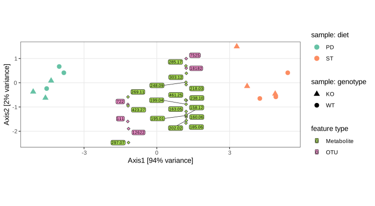
fig_9_32. Download: PDF · SVG9.6.6 Canonical (or constrained) correspondence analysis (CCpnA)
Section 9.6.6 Constrained correspondence analysis (ter Braak 1986; called "canonical correspondence analysis" there, abbreviated CCpnA by the book to avoid a clash with canonical correlation) is a CA in which the sample scores are required to be linear combinations of explanatory variables, here the age bin and the litter of the mice from the dada2 example of Chapter 4.
Filling the gap 9.19: CCpnA as a projection of the CA residuals, and redundancy analysis (PCA-IV) Section 9.6.6 ("it ensures that the resulting CCpnA directions lie in the span of the environmental variables")
Derivation
Constrained CA. Let \(\mathbf{S}\) be the standardised residuals of the samples-by-taxa table (Result 9.4) and \(\mathbf{Z}\) the \(n\times m\) matrix of explanatory variables (dummy-coded factors), centred with the row masses, \(\mathbf{Z}_c\)
Inertia decomposition. By Pythagoras, \(\|\mathbf{S}\|_F^2\)vegan::cca to \(10^{-16}\), checked). The unconstrained part is analysed by an ordinary CA of the residual \((\mathbf{I}-\bm\Pi)\mathbf{S}\).
Redundancy analysis (PCA with instrumental variables). The same construction with a centred continuous table \(\mathbf{Y}\) and no weights is Rao's (1964) PCA-IV, also called redundancy analysis (RDA): the PCA of the fitted values \(\widehat{\mathbf{Y}}\)vegan::rda (checked). CCpnA is the RDA of the chi-square residuals with row weights.
The constrained axes separate the mice by age: the first CCpnA axis distinguishes the young from the older mice, the second separates the oldest group and partly the two litters; a few OTUs (labelled) are outliers on the second axis (Figures 9.33 and 9.34). Following the book the first axis is drawn vertically so that the facets keep a sensible aspect ratio.
Remark: the axis percentages Section 9.6.6, evalProp
The book labels the axes with 100 * CCA$eig / sum(CA$eig), the constrained eigenvalues divided by the unconstrained inertia, which gives 9.9% and 4.1%. As fractions of the total inertia they are 8.5% and 3.5%, and the three constrained axes together carry 14.0%. Our labels use the total.
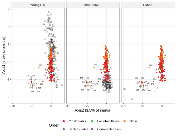
fig_9_33. Download: PDF · SVGQuestion 9.19 (faceting by litter)
Answer
Join the site scores with the sample data, the taxa scores with the taxonomy (the four most abundant orders named, the others "Other"), and facet by family_relationship instead of ageBin: Figure 9.34. The two litters overlap along the first axis but are partly separated along the second.
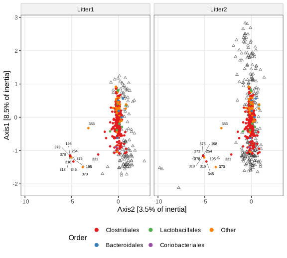
fig_9_34. Download: PDF · SVGThe book's conclusion: the main difference between the communities of these mice lies along the age axis. CCpnA is useful when covariates are available but a fully supervised analysis is too aggressive, and it can use several covariates at once.
Summary of the chapter
- Distances to maps. Classical MDS double-centres the squared distances and takes eigenvectors (Algorithm 9.1). It recovers the points exactly when the distances are Euclidean (Theorem 9.2), coincides with PCA in that case, and is the best least-squares fit to the inner products otherwise (Result 9.3). Negative eigenvalues signal non-Euclidean input.
- Robust maps. Nonmetric MDS uses only the order of the dissimilarities; it minimises Kruskal's stress (whose denominator is the size of the map) by alternating monotone regression and Guttman transforms.
- Supplementary information. Factors are projected onto a PCA as group barycentres; batch effects can be seen this way and removed by centring or by ComBat's empirical Bayes model, provided the biology is not confounded with batch.
- Correspondence analysis is the SVD of standardised residuals; it decomposes \(X^2/n\) along axes, represents chi-square distances, and its biplot has exact barycentric properties in the asymmetric scaling.
- Gradients produce arches and horseshoes because the eigenvectors along a gradient are cosines; the second axis is then a function of the first. Local methods (kernel MDS = kernel PCA, diffusion maps, t-SNE) keep neighbourhoods at the expense of global distances.
- Several tables. The Mantel and RV coefficients measure global association and are tested by permutation (the RV of unrelated tables is about \(\sqrt{\beta_X\beta_Y}/(n-1)\), not 0); CCA is an SVD that overfits whenever \(p+q\ge n\); sparse CCA, RDA and constrained CA regularise or constrain it.
Exercises
The eight exercises of Holmes and Huber (2019), Section 9.9, restated in my own words, with worked solutions (hidden). The numbers come from the chapter's R code (part B, which also draws Figures 9.35 to 9.41).
Exercise 9.1 (presence and absence in the Phylochip data). Replace the Phylochip abundances by presence (value above 8.633) or absence, which keeps about 3,000 taxa present, run a correspondence analysis of the binary taxa-by-samples table, and compare the sample map with Figure 9.15.
Solution
Taxa that are absent everywhere have zero mass and do not affect CA (their profile is undefined, their contribution to every sum is zero), so they can be dropped first; 3,486 taxa remain. The CA eigenvalues decay slowly (Figure 9.35a: 12.9% and 11.1% for the first two axes), as is typical for sparse 0/1 tables, where much of the chi-square is noise. The map of the samples (the columns, Figure 9.35b) tells the same story as the rank-based PCA: the day 2 samples are separated from days 1 and 3 along the first axis, and day 3 sits with day 1. Presence and absence alone therefore carry the protocol effect. CA on binary data compares samples by which taxa they detect, weighting rare detections more (chi-square metric), which makes it sensitive to the detection threshold.
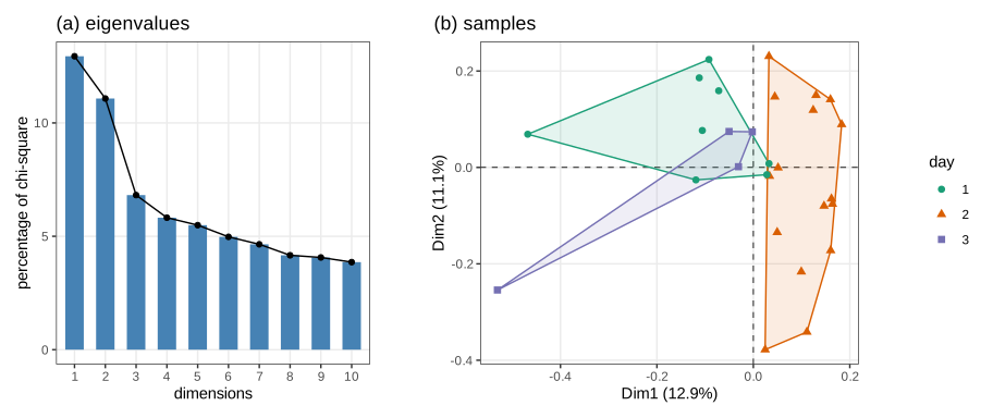
Figure 9.35. Correspondence analysis of the presence and absence Phylochip data: (a) eigenvalues as percentages of the chi-square; (b) the samples, coloured by day, with convex hulls. Reproduces Holmes and Huber (2019), Figure 9.35. Code: ch09_heterogeneous_data_b.R, fig_9_35. Download: PDF · SVGExercise 9.2 (colours and emotions). Table 9.4 of the book counts search-engine hits (in thousands) for pairs of an emotion word (quiet, angry, clever, depressed, happy, lively, perplexed, virtuous) and a colour word (black, blue, green, grey, orange, purple, white). Analyse it by correspondence analysis and describe the biplot.
Solution
The table is dominated by "happy" (54 million of the 98 million hits), but CA works with profiles, so the size of a row only sets its weight. The first axis carries 76.1% of the inertia and the second 20.4% (Figure 9.36). Along the first axis "happy" and "black" lie on one side and "grey" and "purple" on the other, with "quiet", "clever" and "lively" towards grey and "angry" near orange; the second axis separates "depressed", "perplexed" and "virtuous", which co-occur relatively often with "white", from "purple" and "angry". Two cautions: hit counts are not independent observations, so the chi-square statistic (about 2.5 million on the raw counts) cannot be used for a test, only as a measure of departure from proportionality; and co-occurrences in web text reflect phrases ("black Friday", "white lies") as much as perception.
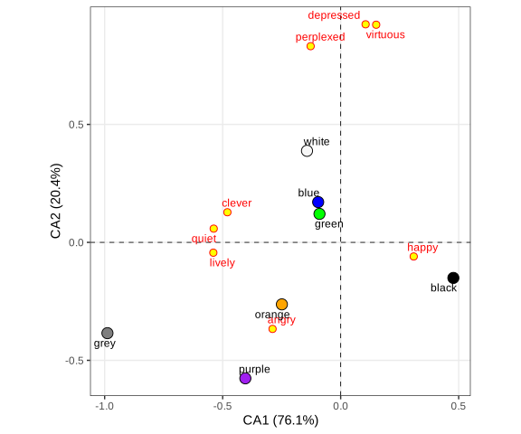
Figure 9.36. Symmetric CA biplot (vegan scaling 3) of the colour and emotion co-occurrence table. Reproduces Holmes and Huber (2019), Figure 9.36. Code: ch09_heterogeneous_data_b.R, fig_9_36. Download: PDF · SVGExercise 9.3 (dating Plato's works). The table
platofgives, for seven works of Plato (Republic, Laws, Critias, Philebus, Politicus, Sophist, Timaeus), the frequencies of the 32 possible patterns of long and short syllables in the last five syllables of a sentence. From a CA biplot, guess the chronological order, knowing that the Republic is the earliest and the Laws the latest; say which endings Plato used more in his early period; and give the percentage of inertia shown by the plane.Solution
The first axis carries 68.8% of the inertia and the second 16.0%, so the plane shows 84.8% (the book's cumulative percentages are 69, 85, 92, 96, 98, 100, and the total inertia is 0.1326; checked). The column points lie on an arch (Section 9.5), from the Republic (axis 1 = 0.37) through Timaeus (0.19), Sophist (0.07), Critias (0.04) and Politicus (\(-0.20\)) to Philebus (\(-0.31\)) and the Laws (\(-0.30\)), the last two separated by the second axis. Following the arch from the Republic to the Laws gives the order Republic, Timaeus, Sophist, Critias, Politicus, Philebus, Laws. The endings with the largest positive first coordinates, on the Republic's side, were used relatively more early:
-uu--,-uu-u,u-uu-,--uu-andu-u--; for instance-uu--is 4.2% of the Republic's endings but 0.6% of those of the Laws. Seriation along an arch assumes that style changed gradually and monotonically, which is a hypothesis, not a fact.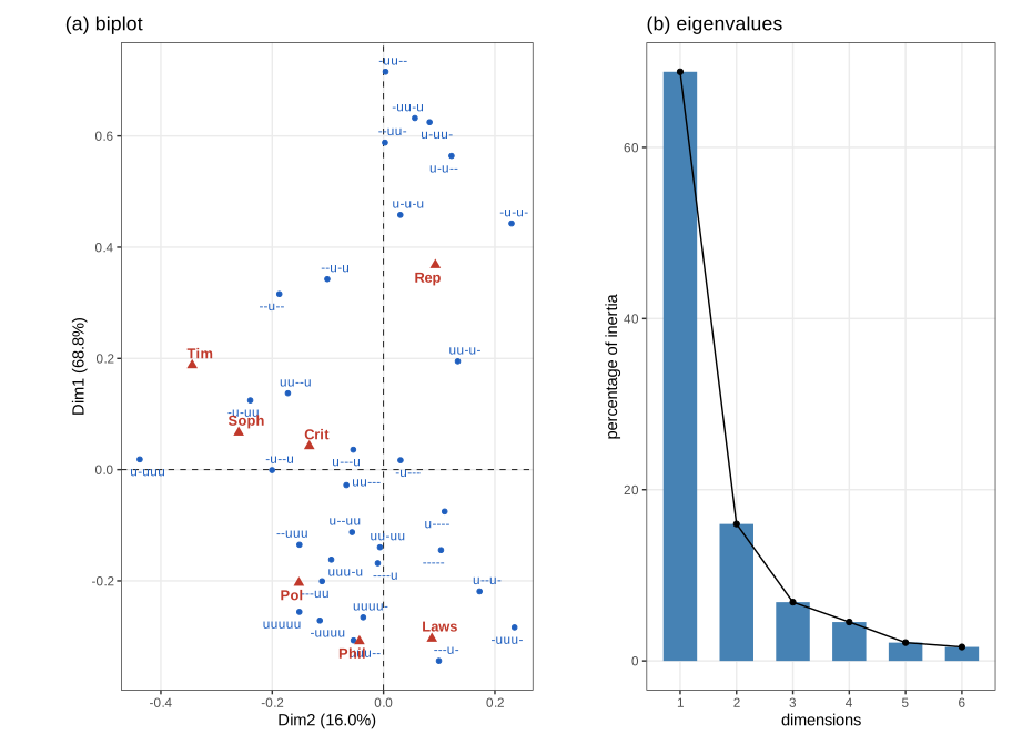
Figure 9.37. CA of Plato's sentence endings: (a) biplot with the first axis drawn vertically, works in red and endings in blue; (b) eigenvalues. Reproduces Holmes and Huber (2019), Figure 9.37. Code: ch09_heterogeneous_data_b.R, fig_9_37. Download: PDF · SVGExercise 9.4 (CA and PCA on a gradient, with and without a perturbation). The lake data come in two versions,
lakelikeand a perturbedlakelikeh. Compare CA and PCA on both, in two dimensions.Solution
The two tables differ only in location 4, whose counts are all multiplied by 10 in
lakelikeh: same profile, ten times the total. Onlakelikeboth methods show the arch; CA explains 56.2% and 24.7%, PCA 51.2% and 23.4%. OnlakelikehPCA is taken over by the heavy location: its first axis (74.4% of the variance) is essentially location 4 against all others (score 10.0 against values between \(-1.5\) and \(-0.9\)), and the gradient is pushed to the second axis. CA depends on rows only through their profiles and masses, so the perturbation only increases the weight of location 4: the arch and the order of the locations survive (64.7% and 20.4%), with location 4 at its place on the arch. This is a practical argument for CA (or for profiles) when samples differ in total abundance, such as sequencing depth.Exercise 9.5 (Moignard raw data). Redo the MDS of Section 9.5.1 on the raw (not normalised) qPCR values and compare.
Solution
On the raw data the first two MDS axes carry 0.776 of the sum of the eigenvalues with \(\ell_1\) distances and 0.630 with \(L_2\) distances (book: 0.776 and 0.630), against 0.781 and 0.574 for the normalised data (checked). The \(\ell_1\) caveat of the remark in Section 9.5.1 applies to both. The maps (run
moignard_mds()in the R code) show the same organisation, so the main structure is not created by the normalisation; the normalisation mainly reduces the share of the second axis in the \(L_2\) analysis.Exercise 9.6 (kernel MDS). Compute kernelised dissimilarities for the Moignard data with Laplace and Gaussian kernels (
kernlab), run MDS on them, compare the variability carried by the first four components, and look for a projection in which the 4SFG\(^-\) (purple) cells branch off.Solution
With the book's settings (Laplace \(\sigma=1/3934\), Gaussian \(\sigma=(1/3934)^2\), and \(1-k\) passed to
cmdscale), the first four components carry, as a percentage of the positive eigenvalues, 71.4% (Laplace) and 74.4% (Gaussian) on the raw data and 65.4% and 67.8% on the normalised data. As explained in Filling the gap 9.13, at these bandwidths the Laplace dissimilarity is a multiple of the Euclidean distance and the Gaussian one a multiple of the squared distance, so these are not local analyses (and the Gaussian version has thousands of negative eigenvalues). Figure 9.38 shows the first three Gaussian kernel axes from two angles; a purple branch is visible along the third axis in (b). To see a genuinely local analysis, set \(\sigma\) near \(1/\text{median}(d^2)\) and use \(\sqrt{2(1-k)}\) as the distance (kernel PCA).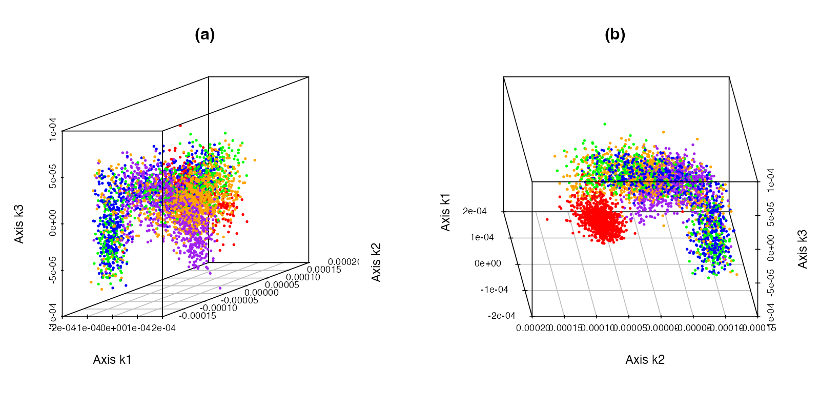
Figure 9.38. Kernel MDS (Gaussian kernel, book's settings) of the normalised cell data: the first three axes from two viewing angles. Reproduces Holmes and Huber (2019), Figure 9.38. Code: ch09_heterogeneous_data_b.R, fig_9_38. Download: PDF · PNGExercise 9.7 (which axis isolates the 4SG cells; principal curves). Map the expression of the ten most variable genes onto 3-d views of the kernel MDS (or diffusion map) coordinates; find which axis best separates the 4SG (red) cells; then fit local principal curves (
LPCM::lpc) through three of the diffusion coordinates.Solution
The ten most variable genes are HbbbH1, Cdh5, Fli1, Kdr, Etv2, Lyl1, Meis1, Gfi1b, Sox7 and Hhex (variances 74 to 33); colouring the cells by any of them (for instance the embryonic globin HbbbH1) is done by replacing the cell-type colours with a colour ramp of the gene's values. To quantify "which axis clusters the 4SG cells", compute for each axis the standardised difference between the mean of the 4SG cells and the mean of the others: for the kernel MDS axes 1 to 4 it is 1.20, 1.61, 0.24 and 0.11, so the second axis separates them best; for the diffusion map on \(\ell_1\) distances the first diffusion coordinate does (2.19). A local principal curve through diffusion coordinates 1, 3 and 4 (bandwidth \(h=0.5\)) follows the main path of the cells from the PS cells to the red branch (Figure 9.39); a larger bandwidth (\(h=0.7\)) gives a smoother curve (Figure 9.40).
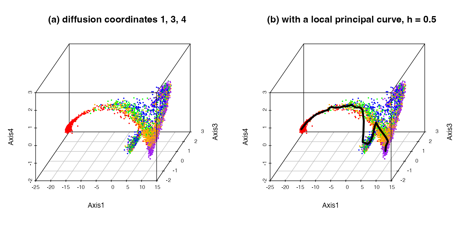
Figure 9.39. Diffusion map of the cells (\(\ell_1\) distances), coordinates 1, 3 and 4: (a) the cells; (b) with the local principal curve for bandwidth \(h=0.5\). Static versions of the book's interactive views. Reproduces Holmes and Huber (2019), Figure 9.39. Code: ch09_heterogeneous_data_b.R, fig_9_39. Download: PDF · PNG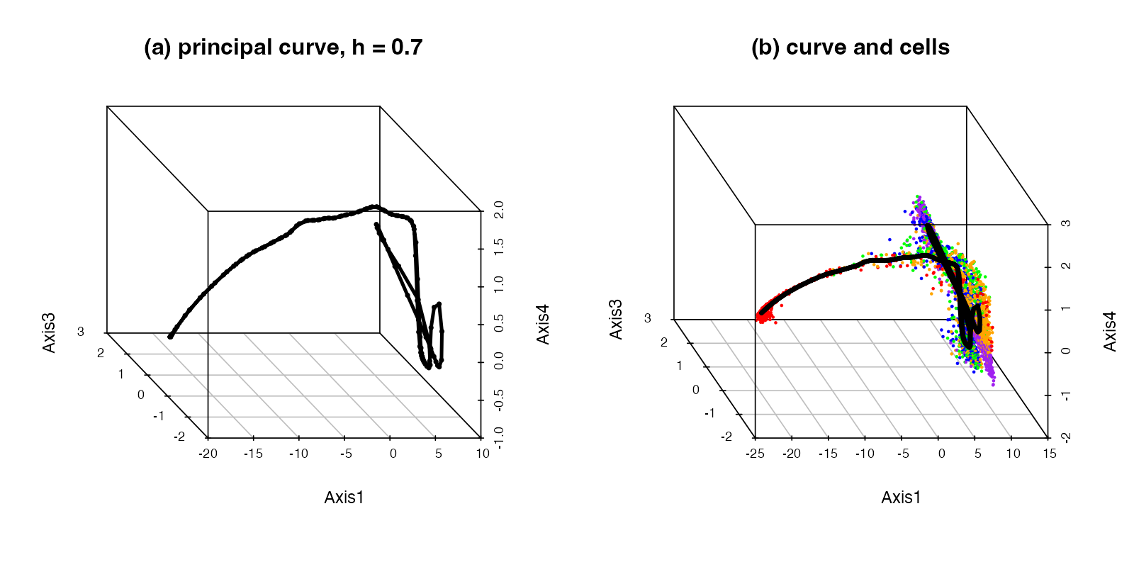
Figure 9.40. The local principal curve for \(h=0.7\): (a) alone, (b) with the cells. Reproduces Holmes and Huber (2019), Figure 9.40. Code: ch09_heterogeneous_data_b.R, fig_9_40. Download: PDF · PNGExercise 9.8 (diffusion maps on \(\ell_1\) and \(L_2\) distances). Diffusion maps estimate distances only locally and turn them into transition probabilities of a random walk; the eigenvectors of the transition matrix give the coordinates. Compare
diffusionMap::diffuseon the \(\ell_1\) and \(L_2\) distances of Section 9.5.1.Solution
diffusechooses the kernel scale \(\varepsilon\) from the data (10,484 for \(\ell_1\), 974 for \(L_2\): squared distances are on very different scales) and forms the Markov matrix \(\mathbf{M}=\mathbf{D}^{-1}\mathbf{K}\) with \(K_{ij}=\exp(-d_{ij}^2/\varepsilon)\); the coordinates are \(\lambda_k^t\bm\psi_k\) for the right eigenvectors \(\bm\psi_k\) after the trivial one. The leading eigenvalues are 0.93, 0.86, 0.49, 0.39 for \(\ell_1\) and 0.65, 0.54, 0.23, 0.17 for \(L_2\), so the \(\ell_1\) walk diffuses more slowly and keeps more structure in the first two coordinates. Nevertheless the coordinates agree: the absolute correlations between corresponding coordinates of the two maps are 0.94, 0.97, 0.98 and 0.98. Both show the trajectory from the PS cells to the two four-somite branches, with the red 4SG branch most clearly separated (Figure 9.41).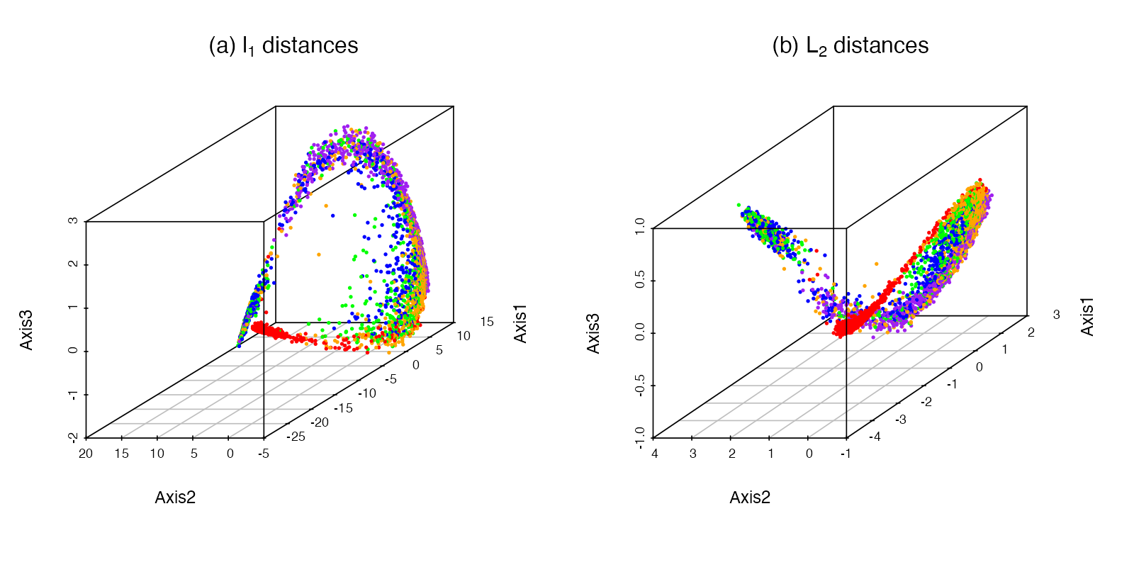
Figure 9.41. The first three diffusion coordinates computed from (a) \(\ell_1\) and (b) \(L_2\) distances between cells. Reproduces Holmes and Huber (2019), Figure 9.41. Code: ch09_heterogeneous_data_b.R, fig_9_41. Download: PDF · PNG
Demonstrations for this chapter
Each demonstration runs in the browser on the chapter's data (exported by the R code) and reproduces the R values, and links back to these notes.
| Demonstration | What you can see |
|---|---|
| Classical and nonmetric MDS | Double centring and all eigenvalues of the Ukraine distances and of Ekman's colours; Algorithm 9.2 step by step with the stress and the Shepard plot; one corrupted object. Presets: 1 Ukraine; 2 Ekman, classical; 3 Ekman, nonmetric; 4 a corrupted city; 5 a one-dimensional map. |
| Correspondence analysis | The standardised residuals of a contingency table, the decomposition of \(X^2/n\) along the axes, and the biplot in symmetric, row-principal and column-principal scaling. Presets: 1 hair and eye colour; 2 barycentres; 3 Plato; 4 colours and emotions; 5 the lake gradient. |
| The horseshoe effect | Simulated species along a gradient (or the lake data): CA, PCA or kernel maps, the cosine eigenvectors and the parabola. Presets: 1 lake data; 2 simulated gradient; 3 narrow niches with PCA: a horseshoe; 4 the same table with CA; 5 the exponential kernel. |
| RV coefficient and sparse CCA | The microbe and metabolite tables: RV with its permutation distribution, sparse CCA with adjustable penalties, and the overfitting of ordinary CCA. Presets: 1 RV test; 2 sparse CCA at the book's penalties; 3 weaker penalties; 4 ordinary CCA overfits. |
The R code that produces every figure of this page is in code/ch09_heterogeneous_data_a.R (Figures 9.1 to 9.25) and code/ch09_heterogeneous_data_b.R (Figures 9.27 to 9.41) (see the code index).
References
- Holmes, S. and Huber, W. (2019). Modern Statistics for Modern Biology. Cambridge University Press. Chapter 9.
- Borg, I. and Groenen, P. J. F. (2005). Modern Multidimensional Scaling: Theory and Applications, 2nd edition. Springer, New York.
- de Leeuw, J. (1977). Applications of convex analysis to multidimensional scaling. In Recent Developments in Statistics (eds J. R. Barra et al.), 133–145. North-Holland, Amsterdam.
- Diaconis, P., Goel, S. and Holmes, S. (2008). Horseshoes in multidimensional scaling and local kernel methods. Annals of Applied Statistics, 2(3), 777–807. doi:10.1214/08-AOAS165.
- Ekman, G. (1954). Dimensions of color vision. The Journal of Psychology, 38(2), 467–474.
- Escoufier, Y. (1973). Le traitement des variables vectorielles. Biometrics, 29(4), 751–760.
- Escoufier, Y. (1987). The duality diagram: a means for better practical applications. In Developments in Numerical Ecology (eds P. Legendre and L. Legendre), 139–156. Springer, Berlin.
- Greenacre, M. J. (2007). Correspondence Analysis in Practice, 2nd edition. Chapman and Hall/CRC.
- Guillot, G. and Rousset, F. (2013). Dismantling the Mantel tests. Methods in Ecology and Evolution, 4(4), 336–344.
- Holmes, S. (2006). Multivariate analysis: the French way. In Probability and Statistics: Essays in Honor of David A. Freedman (eds D. Nolan and T. Speed), IMS Lecture Notes Monograph Series 56.
- Holmes, S., Alekseyenko, A. V., Timme, A., Nelson, T., Pasricha, P. J. and Spormann, A. (2011). Visualization and statistical comparisons of microbial communities using R packages on Phylochip data. Pacific Symposium on Biocomputing, 142–153.
- Hotelling, H. (1936). Relations between two sets of variates. Biometrika, 28(3/4), 321–377.
- Johnson, W. E., Li, C. and Rabinovic, A. (2007). Adjusting batch effects in microarray expression data using empirical Bayes methods. Biostatistics, 8(1), 118–127. doi:10.1093/biostatistics/kxj037.
- Josse, J. and Holmes, S. (2016). Measuring multivariate association and beyond. Statistics Surveys, 10, 132–167.
- Josse, J., Pagès, J. and Husson, F. (2008). Testing the significance of the RV coefficient. Computational Statistics and Data Analysis, 53(1), 82–91.
- Kashyap, P. C., Marcobal, A., Ursell, L. K. et al. (2013). Genetically dictated change in host mucus carbohydrate landscape exerts a diet-dependent effect on the gut microbiota. PNAS, 110(42), 17059–17064.
- Kazi-Aoual, F., Hitier, S., Sabatier, R. and Lebreton, J.-D. (1995). Refined approximations to permutation tests for multivariate inference. Computational Statistics and Data Analysis, 20(6), 643–656.
- Kendall, D. G. (1969). Incidence matrices, interval graphs and seriation in archeology. Pacific Journal of Mathematics, 28(3), 565–570.
- Kruskal, J. B. (1964). Multidimensional scaling by optimizing goodness of fit to a nonmetric hypothesis. Psychometrika, 29(1), 1–27. doi:10.1007/BF02289565.
- Leek, J. T., Scharpf, R. B., Corrada Bravo, H. et al. (2010). Tackling the widespread and critical impact of batch effects in high-throughput data. Nature Reviews Genetics, 11(10), 733–739. doi:10.1038/nrg2825.
- van der Maaten, L. and Hinton, G. (2008). Visualizing data using t-SNE. Journal of Machine Learning Research, 9, 2579–2605.
- Moignard, V., Woodhouse, S., Haghverdi, L. et al. (2015). Decoding the regulatory network of early blood development from single-cell gene expression measurements. Nature Biotechnology, 33, 269–276. doi:10.1038/nbt.3154.
- Perraudeau, F., Risso, D., Street, K., Purdom, E. and Dudoit, S. (2017). Bioconductor workflow for single-cell RNA sequencing: normalization, dimensionality reduction, clustering, and lineage inference. F1000Research, 6, 1158.
- Rao, C. R. (1964). The use and interpretation of principal component analysis in applied research. Sankhyā A, 26(4), 329–358.
- Rhee, S.-Y., Gonzales, M. J., Kantor, R., Betts, B. J., Ravela, J. and Shafer, R. W. (2003). Human immunodeficiency virus reverse transcriptase and protease sequence database. Nucleic Acids Research, 31(1), 298–303.
- Schölkopf, B., Smola, A. and Müller, K.-R. (1998). Nonlinear component analysis as a kernel eigenvalue problem. Neural Computation, 10(5), 1299–1319. doi:10.1162/089976698300017467.
- Schoenberg, I. J. (1935). Remarks to Maurice Fréchet's article "Sur la définition axiomatique d'une classe d'espaces distanciés vectoriellement applicables sur l'espace de Hilbert". Annals of Mathematics, 36(3), 724–732.
- ter Braak, C. J. F. (1986). Canonical correspondence analysis: a new eigenvector technique for multivariate direct gradient analysis. Ecology, 67(5), 1167–1179.
- Witten, D. M., Tibshirani, R. and Hastie, T. (2009). A penalized matrix decomposition, with applications to sparse principal components and canonical correlation analysis. Biostatistics, 10(3), 515–534. doi:10.1093/biostatistics/kxp008.
- Young, G. and Householder, A. S. (1938). Discussion of a set of points in terms of their mutual distances. Psychometrika, 3(1), 19–22.