Statistical Learning
Statistical learning is the business of estimating an unknown relationship \(Y=f(X)+\varepsilon\) from data, either to predict \(Y\) or to understand how it depends on \(X\). This chapter sets up the vocabulary used in the rest of the book (prediction and inference, parametric and non-parametric methods, supervised and unsupervised learning, regression and classification) and the two ideas that govern everything after it: a method must be judged on new data, not on the data it was fitted to, and its error on new data splits into an irreducible part, a squared bias and a variance that pull in opposite directions as the method becomes more flexible. The classification version of the same story leads to the Bayes classifier and to K-nearest neighbours. The lab introduces R and Python side by side.
Ch. 1 Introduction Ch. 2 Statistical learning Ch. 3 Linear regression Ch. 4 Classification Ch. 5 Resampling Ch. 6 Selection and regularization Ch. 7 Beyond linearity Ch. 8 Trees Ch. 9 SVMs Ch. 10 Deep learning Ch. 11 Survival analysis Ch. 12 Unsupervised learning Ch. 13 Multiple testing
How to read these notes
They follow the book. Sections carry the book's numbers (2.1.1, 2.2.2, ...) and displayed equations that appear in the book carry its equation numbers, e.g. \((2.7)\), so the notes can be read next to either edition. Equations without a number are steps the book leaves out.
Filling the gaps. The book is written for readers without much mathematics and says, for example, that the bias-variance decomposition (2.7) is "beyond the scope of this book". Each such place has an orange Filling the gap box with the argument written out at the level of a first course in probability. The derivations start hidden: open one with its bar, or use the button below. Nothing later in the course depends on reading them, but they explain why the pictures look the way they do.
Figures, code and demonstrations. Every figure of the chapter that is computed from data or from a simulation is recomputed by the Python code (Figure 2.7, a hand-drawn schematic, is replaced by a table). The book's simulations are not published, so the simulated figures use simulations of the same kind; their settings are stated in the captions. The ▶ Demo boxes open an interactive demonstration set to the case being discussed. The lab (Section 2.3) shows the R and the Python code side by side.
Main reference
G. James, D. Witten, T. Hastie and R. Tibshirani, An Introduction to Statistical Learning with Applications in R, 2nd edition, Springer (2021), Chapter 2, pages 15–57; and G. James, D. Witten, T. Hastie, R. Tibshirani and J. Taylor, An Introduction to Statistical Learning with Applications in Python, Springer (2023), Chapter 2, pages 15–67. The two editions share the text, figures and exercises of the chapter and differ in the lab. Book website, with the data sets: www.statlearning.com. Section, equation, figure and exercise numbers below refer to these books; page numbers are those of the R edition unless stated.
The explanations, derivations, figures and code are my own; equations are cited by their numbers in the book.
Companion courses
This course is the applied, introductory member of a family. The same ideas are treated with more mathematics in:
- Statistical Learning: Theory and Methods (Hastie, Tibshirani and Friedman 2009), the graduate course on the same authors' larger book: Chapter 2 (least squares and nearest neighbours, statistical decision theory, the curse of dimensionality, the bias-variance trade-off) and Chapter 7 (model assessment and selection). Links marked Deeper below go to the matching section.
- Bayesian and Probabilistic Machine Learning (Bishop 2006): overfitting in polynomial curve fitting and decision theory, Chapter 1; the bias-variance decomposition, Section 3.2.
- Foundations of Deep Learning (Bishop and Bishop 2024): decision theory for regression and the bias-variance trade-off, Sections 4.2–4.3.
The chapter at a glance
- 2.1 The model \(Y=f(X)+\varepsilon\) (Definition 2.1). For any estimate \(\hat f\), the expected squared prediction error is a reducible part \((f-\hat f)^2\) plus the irreducible \(\Var(\varepsilon)\) (Result 2.1), and \(f(x)=\E(Y\given X=x)\) is the best possible predictor (Result 2.2). Parametric methods assume a form for \(f\) and estimate a few parameters; non-parametric methods, such as the thin-plate spline, let the data choose the shape and can fit the training data perfectly.
- 2.2.1 The training MSE always falls as flexibility grows (for smoothing splines this is Result 2.3), and for a linear smoother it underestimates the error on new responses by exactly \(2\sigma^2\df/n\) on average. The test MSE is what matters, and it is U-shaped.
- 2.2.2 Expected test MSE = variance + squared bias + \(\Var(\varepsilon)\) (2.7), proved in Filling the gap 2.5; for a smoothing spline all three are computed exactly (Result 2.4, Figure 2.12).
- 2.2.3 The Bayes classifier, which picks the most probable class, has the smallest possible error rate, \(1-\E\max_j\Pr(Y=j\given X)\) (Result 2.5). K-nearest neighbours (Definition 2.3) imitates it; \(K\) plays the role of (inverse) flexibility.
- 2.3 The lab: R and Python basics, arrays and indexing, graphics, loading and summarising the
Autodata, with the two languages side by side.
2.1 What Is Statistical Learning?
pp. 15–17 The chapter opens with a consulting problem. The Advertising data record, for 200 markets, the sales of a product (in thousands of units) and the budgets spent advertising it on TV, radio and in newspapers (in thousands of dollars). The client cannot set sales directly, but can set the three budgets; so the questions are whether, and how, sales depend on them. The budgets are the inputs (also called predictors, features, independent variables), written \(X_1,X_2,X_3\); sales is the output (response, dependent variable), written \(Y\).
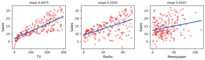
Advertising data: sales against each budget separately, with the least-squares line of sales on that budget alone. The slopes (0.0475, 0.2025 and 0.0547 thousand units per thousand dollars) and intercepts (7.03, 9.31, 12.35) are those of the book's Tables 3.1 and 3.3. Code: ch02_statistical_learning.py, fig_2_1. Reproduces James et al. (2021), Figure 2.1. Download: PDF · SVGDefinition 2.1 (the general model) p. 16, (2.1)
With a quantitative response \(Y\) and predictors \(X=(X_1,\dots,X_p)\), statistical learning assumes
\[ Y=f(X)+\varepsilon, \tag{2.1} \]where \(f\) is a fixed but unknown function (the systematic part: what \(X\) tells us about \(Y\)) and \(\varepsilon\) is a random error term, independent of \(X\), with mean zero. Statistical learning is the collection of methods for estimating \(f\) from data.
Two things in (2.1) are assumptions, not facts about the world: that the error is added to \(f(X)\), and that it is independent of \(X\) (so its spread does not change with \(X\)). They make the analysis clean; later chapters relax them where needed. Note also that (2.1) always holds in a weaker sense: whatever the joint distribution of \((X,Y)\), we can define \(f(x)=\E(Y\given X=x)\) and \(\varepsilon=Y-f(X)\); then \(\E(\varepsilon\given X)=0\) automatically, although \(\varepsilon\) need not be independent of \(X\).
pp. 16–17 The Income data illustrate (2.1) with one and two inputs: income (in tens of thousands of dollars) against years of education for 30 people, and against education and seniority. These data were simulated by the authors, so for them \(f\) is known; but the book does not publish \(f\). In Figures 2.2 and 2.3 below, a smooth curve and a smooth surface fitted to the data stand in for it.
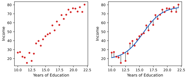
Income1 data. Left: income against years of education for 30 individuals. Right: a smooth curve playing the role of the true \(f\), and the errors \(\varepsilon_i\) as vertical segments; some are positive, some negative, and they average about zero. The curve is the logistic function \(a+b/(1+e^{-(x-c)/s})\) fitted by least squares (\(a=18.9\), \(b=59.4\), \(c=15.7\), \(s=1.73\)), a stand-in for the authors' unpublished \(f\). Reproduces James et al. (2021), Figure 2.2. Download: PDF · SVG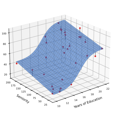
Income2 data: income as a function of years of education and seniority. The blue surface stands in for the true \(f\): the S-shaped curve in education plus a linear term in seniority, 17.3 + 57.8 / (1 + exp(−(education − 16.2)/1.24)) + 0.144 × seniority, fitted by least squares. Reproduces James et al. (2021), Figure 2.3. Download: PDF · SVG2.1.1 Why Estimate f?
pp. 17–19 Prediction. When \(X\) is easy to measure but \(Y\) is not (yet), we predict \(Y\) by
\[ \hat Y=\hat f(X), \tag{2.2} \]using the fact that the error averages to zero. For prediction, \(\hat f\) may be a black box: only the accuracy of \(\hat Y\) matters.
Result 2.1 (reducible and irreducible error) p. 19, (2.3)
Fix an estimate \(\hat f\) and a value \(X=x\), so that the only randomness is in \(\varepsilon\). Then
\[ \E(Y-\hat Y)^2=\E\big[f(x)+\varepsilon-\hat f(x)\big]^2=\underbrace{\big[f(x)-\hat f(x)\big]^2}_{\text{reducible}}+\underbrace{\Var(\varepsilon)}_{\text{irreducible}}. \tag{2.3} \]The first term can be made small by estimating \(f\) better; the second cannot be reduced by any choice of \(\hat f\), and is a floor for the expected squared error of every prediction based on \(X\).
Filling the gap 2.1: the algebra behind (2.3), and a version with everything random p. 19, "it is easy to show"
One expansion of a square, and one fact: \(\E\varepsilon=0\).
Derivation
Write \(a=f(x)-\hat f(x)\), a fixed number once \(x\) and \(\hat f\) are fixed. Then \(Y-\hat Y=a+\varepsilon\) and
\[ \E(a+\varepsilon)^2=a^2+2a\,\E\varepsilon+\E\varepsilon^2=a^2+\Var(\varepsilon), \]because \(\E\varepsilon=0\) kills the middle term and makes \(\E\varepsilon^2=\Var(\varepsilon)+(\E\varepsilon)^2=\Var(\varepsilon)\).
With \(X\) random and \(\hat f\) estimated from data. In practice \(\hat f\) comes from a training set and \(X\) is a new random input. If the new error \(\varepsilon\) is independent of the new \(X\) and of the training set (it is noise in a new observation), apply the argument conditionally on \(X\) and on the training set, then average:
\[ \E\big(Y-\hat f(X)\big)^2=\E\big[f(X)-\hat f(X)\big]^2+\Var(\varepsilon)\ \ge\ \Var(\varepsilon). \]So no method, however clever, has expected squared prediction error below \(\Var(\varepsilon)\): that is the dashed line in Figures 2.9–2.12. (Confirmed numerically by simulation.) ∎
Result 2.2 (the best possible predictor is the conditional mean)
Among all functions \(g\), the expected squared error \(\E\big(Y-g(X)\big)^2\) is smallest for \(g(x)=\E(Y\given X=x)\), and under (2.1) this is exactly \(f(x)\). So \(f\) is not just "a" relationship between \(X\) and \(Y\): it is the target that every regression method in the book is trying to estimate, and \(\Var(\varepsilon)\) is the smallest achievable expected squared error.
Filling the gap 2.2: why the conditional mean wins
The book takes \(f\) as the goal without saying why; the reason is a decomposition of the same kind as (2.3).
Derivation
Let \(m(x)=\E(Y\given X=x)\). For any \(g\),
\[ \E\big(Y-g(X)\big)^2=\E\big(Y-m(X)\big)^2+\E\big(m(X)-g(X)\big)^2+2\,\E\Big[\big(Y-m(X)\big)\big(m(X)-g(X)\big)\Big]. \]The cross term is zero: conditionally on \(X\), the factor \(m(X)-g(X)\) is a constant and \(\E\big(Y-m(X)\given X\big)=0\); averaging a zero conditional expectation gives zero (the tower property). The middle term is \(\ge0\) and vanishes only when \(g=m\) (almost everywhere). Under (2.1), because \(\varepsilon\) is independent of \(X\) with mean zero,
\[ m(x)=\E\big(f(x)+\varepsilon\given X=x\big)=f(x)+\E\varepsilon=f(x), \]and then \(\E(Y-m(X))^2=\Var(\varepsilon)\). ∎
Deeper: Statistical Learning: Theory and Methods, Result 2.3 (statistical decision theory, Section 2.4), which also treats absolute loss (giving the conditional median) and the classification loss.
See also (companion courses): the regression function is the conditional mean; the conditional mean minimises the expected squared loss.
pp. 19–20 Inference. Often the goal is to understand how \(Y\) depends on \(X\) rather than to predict it: which predictors matter, whether each effect is positive or negative, whether it depends on the other predictors, whether a linear form is good enough. Then \(\hat f\) cannot be a black box. For the Advertising data, inference questions are: which media are associated with sales, which gives the largest boost, and how much do sales rise per extra thousand dollars of TV advertising. Predicting the response to a mailing from demographic variables is a prediction problem; asking how much a river view adds to the price of a house is an inference problem; many problems are both. Simple, linear methods make inference easy but may predict less accurately than highly non-linear ones; that tension returns in Section 2.1.3.
2.1.2 How Do We Estimate f?
pp. 21–22 We observe \(n\) training pairs \(\{(x_1,y_1),\dots,(x_n,y_n)\}\), with \(x_i=(x_{i1},\dots,x_{ip})^\T\), and want \(\hat f\) with \(Y\approx\hat f(X)\) for new pairs as well. Most methods are either parametric or non-parametric.
Parametric methods work in two steps: (1) assume a form for \(f\), for example the linear model
\[ f(X)=\beta_0+\beta_1X_1+\beta_2X_2+\cdots+\beta_pX_p, \tag{2.4} \]and (2) fit it, here by choosing \(\beta_0,\dots,\beta_p\) so that \(Y\approx\beta_0+\beta_1X_1+\cdots+\beta_pX_p\) on the training data, usually by least squares (Chapter 3). Estimating \(p+1\) numbers is far easier than estimating an arbitrary function of \(p\) variables. The price is that the assumed form may be wrong; a more flexible form needs more parameters, and with too many the fit starts to follow the noise (overfitting).
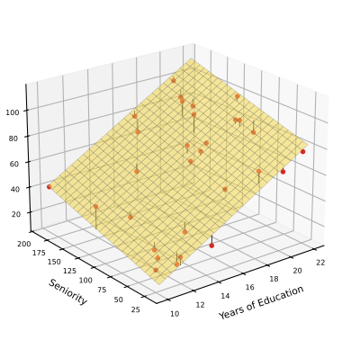
Income2 data: predicted income = −50.09 + 5.896 × education + 0.1729 × seniority. The plane captures the positive effect of both inputs but not the S-shaped dependence on education. Reproduces James et al. (2021), Figure 2.4. Download: PDF · SVGpp. 23–24 Non-parametric methods make no explicit assumption about the form of \(f\); they look for a function close to the data that is not too rough. They can fit a much wider range of shapes, but because they do not reduce the problem to a few parameters they need many more observations. The example is the thin-plate spline (Figures 2.5 and 2.6), whose single tuning parameter sets the level of smoothness.
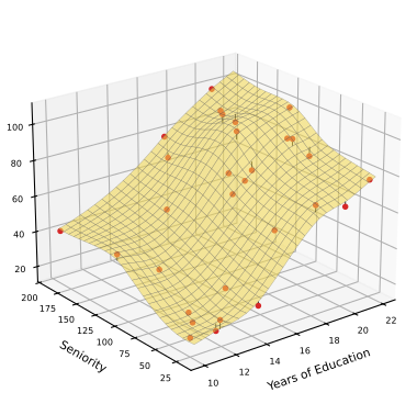
Income2, with the smoothness chosen by generalised cross-validation (about 18 effective degrees of freedom; training MSE 7.2). Reproduces James et al. (2021), Figure 2.5. Download: PDF · SVG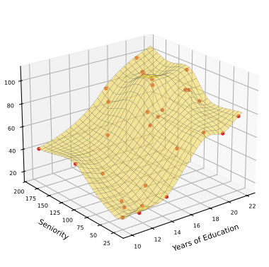
Filling the gap 2.3: what a thin-plate spline is, and what "level of smoothness" means pp. 23–24
A thin-plate spline trades closeness to the data against a measure of bending; one number sets the trade, and the "effective degrees of freedom" measure the result.
Derivation
With two inputs \(x=(x_1,x_2)\), the thin-plate spline minimises
\[ \sum_{i=1}^n\big(y_i-f(x_i)\big)^2+\lambda J(f),\qquad J(f)=\iint\Big[\Big(\frac{\partial^2f}{\partial x_1^2}\Big)^2+2\Big(\frac{\partial^2f}{\partial x_1\partial x_2}\Big)^2+\Big(\frac{\partial^2f}{\partial x_2^2}\Big)^2\Big]\,\d x_1\,\d x_2 . \]\(J(f)\) is the bending energy of a thin metal plate shaped like \(f\); it is zero exactly when all second derivatives vanish, that is when \(f\) is a plane. Hence the two extremes: as \(\lambda\to\infty\) the fit is forced to be a plane, the least-squares plane of Figure 2.4; as \(\lambda\to0\) only the data matter and the fit interpolates them (Figure 2.6), as long as the inputs are distinct. The minimiser has the closed form
\[ \hat f(x)=\beta_0+\beta_1x_1+\beta_2x_2+\sum_{i=1}^n\alpha_i\,\eta(\|x-x_i\|),\qquad \eta(r)=r^2\log r \](Duchon 1977), and its fitted values are linear in the responses: \(\hat\by=\bH_\lambda\by\). The effective degrees of freedom \(\df(\lambda)=\tr\bH_\lambda\) fall from \(n\) (interpolation) to 3 (a plane, three parameters) as \(\lambda\) grows; this is how the "flexibility" of a non-parametric fit is measured.
The numbers here. Education and seniority are rescaled to \([0,1]\) first, since \(J\) is not invariant to stretching one axis. Generalised cross-validation, \(\mathrm{GCV}(\lambda)=n\,\RSS/(n-\df)^2\) (Craven and Wahba 1979), picks \(\df\approx18.1\) with training MSE 7.17 (Figure 2.5); \(\lambda=0\) gives \(\df=30=n\) and training MSE 0 (Figure 2.6). The plane has \(\df=3\). ∎
Deeper: Statistical Learning: Theory and Methods, Section 5.7 (multidimensional splines and thin-plate splines) and Section 5.4.1 (degrees of freedom of a smoother).
2.1.3 The Trade-Off Between Prediction Accuracy and Model Interpretability
pp. 24–26 Linear regression can only produce lines and planes; thin-plate splines can produce almost any smooth surface. Why ever prefer the restrictive method? For inference, because a restrictive model is interpretable: each coefficient of (2.4) says how \(Y\) changes with one predictor. And, more surprisingly, often for prediction too, because flexible methods overfit (Section 2.2). The book's Figure 2.7 places the methods of later chapters on a flexibility-interpretability chart; it is a schematic drawing, so here it is a table.
| Method (chapter) | Flexibility | Interpretability | Why |
|---|---|---|---|
| Subset selection, the lasso (6) | lowest | highest | linear, and only a few predictors keep a nonzero coefficient |
| Least squares (3) | low | high | linear in all predictors |
| Generalised additive models (7) | medium | medium | one smooth curve per predictor, added up |
| Trees (8) | medium | medium | a sequence of yes/no splits that can be drawn |
| Bagging, boosting (8), support vector machines (9) | high | low | averages of many trees, or non-linear kernels |
| Deep learning (10) | highest | lowest | millions of parameters in layered non-linear functions |
Table in place of James et al. (2021), Figure 2.7 (a hand-placed schematic, not computed from data).
2.1.4 Supervised Versus Unsupervised Learning
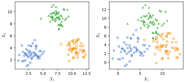
pp. 26–28 In supervised learning every \(x_i\) comes with a response \(y_i\), which "supervises" the fit. In unsupervised learning there are only the \(x_i\); one can still look for structure, for example groups of similar observations (cluster analysis, Chapter 12). With two variables one can just look (Figure 2.8); with \(p\) variables there are \(\binom p2=p(p-1)/2\) scatterplots of pairs (45 for \(p=10\), 1,225 for \(p=50\)), and automatic methods are needed. When only \(m<n\) observations have a response, the problem is semi-supervised, which the book does not cover.
See also: clustering in Statistical Learning: Theory and Methods, Section 14.3.
2.1.5 Regression Versus Classification Problems
pp. 28–29 Variables are quantitative (numbers: age, income, a price) or qualitative, also called categorical (one of \(K\) classes: marital status, brand, default yes/no, a type of leukaemia). A quantitative response makes a regression problem, a qualitative one a classification problem. The line is not sharp: logistic regression (Chapter 4) is used for two-class responses but estimates class probabilities, a regression-like task; K-nearest neighbours and boosting handle both types. The type of the predictors matters less, provided qualitative predictors are coded properly (Chapter 3).
2.2 Assessing Model Accuracy
p. 29 There is no free lunch in statistics: no method beats all others on every data set. Choosing a method for the data at hand is therefore part of the job, and this section sets up how to judge one.
2.2.1 Measuring the Quality of Fit
pp. 29–30 In regression the usual measure is the mean squared error
\[ \MSE=\frac1n\sum_{i=1}^n\big(y_i-\hat f(x_i)\big)^2. \tag{2.5} \]Computed on the data used for fitting, this is the training MSE. What we care about is accuracy on previously unseen data: tomorrow's stock price, not last week's; the diabetes risk of future patients, not of those whose status we already know. For a large set of test observations \((x_0,y_0)\) not used in fitting, the test MSE is
\[ \Ave\big(y_0-\hat f(x_0)\big)^2, \tag{2.6} \]and we want the method with the smallest test MSE. Minimising the training MSE instead is tempting but wrong: many methods fit by making the training MSE small, so it is an optimistic and often badly misleading guide.
pp. 30–33 Figures 2.9–2.11 show this on simulated data, with smoothing splines (Chapter 7) of increasing flexibility. Flexibility is measured by the degrees of freedom, from 2 (a straight line) upwards.
Definition 2.2 (the smoothing spline and its degrees of freedom) pp. 31–32; Chapter 7, (7.11)
For one input, the smoothing spline with tuning parameter \(\lambda\ge0\) is the function \(\hat g\) minimising
\[ \sum_{i=1}^n\big(y_i-g(x_i)\big)^2+\lambda\int g''(t)^2\,\d t . \]Its fitted values are \(\hat\bg=\bS_\lambda\by\) for a matrix \(\bS_\lambda\) (the smoother matrix) that does not depend on \(\by\), and its effective degrees of freedom are \(\df_\lambda=\tr\bS_\lambda\), which fall from \(n\) (\(\lambda=0\), the curve interpolates) to 2 (\(\lambda\to\infty\), the least-squares line).
Filling the gap 2.4: how the smoothing spline is computed deferred by the book to Chapter 7
The figures of this section need the smoothing spline now, so here is the whole computation; it is also what the code and the demonstrations do.
Derivation
Step 1: the minimiser is a natural cubic spline with knots at the \(x_i\). Among all smooth functions taking given values at the (sorted, distinct) points \(x_1<\cdots<x_n\), the natural cubic spline through those values (cubic between knots, twice continuously differentiable, linear outside \([x_1,x_n]\)) has the smallest \(\int g''^2\) (Green and Silverman 1994, Theorem 2.3). Replacing any candidate \(g\) by the natural cubic spline through its values \(g(x_i)\) leaves the sum of squares unchanged and does not increase the penalty, so we may search among natural cubic splines only.
Step 2: the penalty is a quadratic form in the values. Write \(\bg=(g(x_1),\dots,g(x_n))^\T\) and \(h_i=x_{i+1}-x_i\). Let \(\bQ\) be the \(n\times(n-2)\) matrix with nonzero entries \(q_{j-1,j}=1/h_{j-1}\), \(q_{jj}=-1/h_{j-1}-1/h_j\), \(q_{j+1,j}=1/h_j\), and \(\bR\) the \((n-2)\times(n-2)\) tridiagonal matrix with \(r_{jj}=(h_{j-1}+h_j)/3\) and \(r_{j,j+1}=r_{j+1,j}=h_j/6\) (\(j=2,\dots,n-1\)). Then the second derivatives at the interior knots are \(\bgam=\bR^{-1}\bQ^\T\bg\), \(g''\) is piecewise linear between them, and
\[ \int g''(t)^2\,\d t=\bg^\T\bK\bg,\qquad \bK=\bQ\bR^{-1}\bQ^\T . \]Step 3: solve. The criterion is \(\|\by-\bg\|^2+\lambda\bg^\T\bK\bg\), a convex quadratic in \(\bg\); setting its gradient \(-2(\by-\bg)+2\lambda\bK\bg\) to zero gives the Reinsch form
\[ \hat\bg=(\bI+\lambda\bK)^{-1}\by=\bS_\lambda\by . \]Step 4: degrees of freedom. \(\bK\) is symmetric and positive semi-definite; its null space consists of the vectors with zero roughness, the values of straight lines, so it has exactly two zero eigenvalues. With \(\bK=\bU\diag(d_k)\bU^\T\),
\[ \bS_\lambda=\bU\diag\Big(\frac1{1+\lambda d_k}\Big)\bU^\T,\qquad \df_\lambda=\tr\bS_\lambda=\sum_{k=1}^n\frac1{1+\lambda d_k}, \]a decreasing function of \(\lambda\) from \(n\) to 2 (the two zero eigenvalues always contribute 1 each). As \(\lambda\to\infty\), \(\bS_\lambda\) tends to the projection onto the straight lines, the least-squares line. To fit with a given \(\df\), solve \(\df_\lambda=\df\) for \(\lambda\) (by bisection). Between the knots the fitted curve is the natural cubic spline through \(\hat\bg\), so \(\hat g(x_0)=\bl(x_0)^\T\by\) for a weight vector \(\bl(x_0)\): the smoothing spline is a linear smoother.
The numbers here. With the 50 inputs used below, \(\df=5.4\) needs \(\lambda\approx2011\), \(\df=8.7\) needs \(\lambda\approx213\) and \(\df=25\) needs \(\lambda\approx2.0\). The fitted values agree with SciPy's make_smoothing_spline at the same \(\lambda\) and with R's smooth.spline at the same degrees of freedom (confirmed numerically). ∎
Deeper: Statistical Learning: Theory and Methods, Section 5.4 (the smoothing-spline theorem, Result 5.5) and Section 5.4.1 (smoother matrices and degrees of freedom).
The three simulated examples. The book does not publish its simulations, so these are new ones of the same kind. The inputs are 50 fixed points on \([0,100]\), one placed at random in the middle of each of 50 equal bins, and \(Y=f(X)+\varepsilon\) with \(\Var(\varepsilon)=1\). Example 1 has a non-linear \(f\) (rising, then falling); Example 2 an \(f\) close to a straight line; Example 3 an \(f\) far from linear. The right panels show the training MSE and the test MSE averaged over training samples, both computed exactly (Result 2.4 below), against the degrees of freedom; the squares are the training and test MSE of the three fits on the left, which come from one training sample.
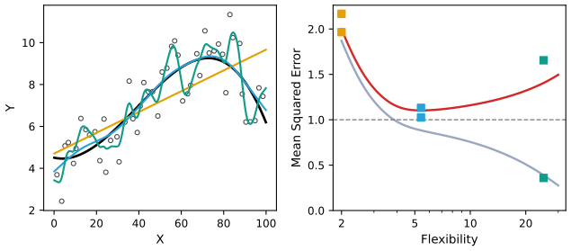
fig_2_9, exact_curves. Reproduces James et al. (2021), Figure 2.9. Download: PDF · SVG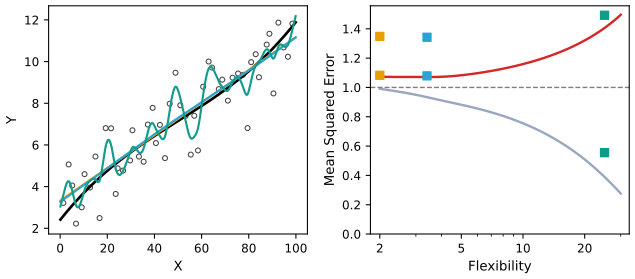
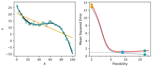
pp. 31–33 The pattern is the same in all three examples: the training MSE falls steadily as flexibility grows, while the test MSE falls, levels off and rises again, a U-shape. A method that has small training MSE but large test MSE is overfitting: it has picked up patterns that are just noise in this particular training set, and that are absent from new data. (Strictly, overfitting means that a less flexible method would have had smaller test MSE.) Where the bottom of the U lies depends on the data: df 3.4, 5.4 and 8.7 in the three examples. In practice \(f\) is unknown and there is usually no test set, so the test MSE has to be estimated from the training data; cross-validation (Chapter 5) is the main tool.
Result 2.3 (why the training MSE keeps falling, and by how much it is too optimistic) pp. 31–32
(a) For smoothing splines, the training residual sum of squares can only fall as \(\lambda\) decreases (flexibility grows). The same holds for least-squares fits as predictors are added to a model.
(b) Fix the inputs, and let a linear smoother \(\hat\by=\bS\by\) be applied to \(\by=\bf+\be\), \(\be\) with independent components of variance \(\sigma^2\). Let \(\by_0=\bf+\be_0\) be new responses at the same inputs, with \(\be_0\) independent of \(\be\). Then
\[ \E\Big[\frac1n\|\by_0-\bS\by\|^2\Big]-\E\Big[\frac1n\|\by-\bS\by\|^2\Big]=\frac{2\sigma^2}{n}\,\tr\bS=\frac{2\sigma^2\df}{n}. \]The training MSE underestimates the error on new responses by an amount that grows with the flexibility. In Example 1, with \(\df=5.4\), \(n=50\), \(\sigma^2=1\), the gap is \(0.216\).
Filling the gap 2.6: the two parts of Result 2.3 p. 32, "we almost always expect the training MSE to be smaller than the test MSE"
Part (a) is an exchange argument between two optimisation problems; part (b) is a computation with \(\E\,\be^\T\mathbf A\be=\sigma^2\tr\mathbf A\).
Derivation
(a) Let \(\lambda_1<\lambda_2\), with fits \(g_1,g_2\), residual sums of squares \(\RSS_1,\RSS_2\) and roughness \(J_1,J_2\). Each fit is optimal for its own \(\lambda\):
\[ \RSS_1+\lambda_1J_1\le\RSS_2+\lambda_1J_2,\qquad \RSS_2+\lambda_2J_2\le\RSS_1+\lambda_2J_1 . \]Adding gives \((\lambda_2-\lambda_1)(J_2-J_1)\le0\), so \(J_2\le J_1\). Then the first inequality gives \(\RSS_1\le\RSS_2+\lambda_1(J_2-J_1)\le\RSS_2\). For least squares, adding a predictor enlarges the set of candidate fits, so the minimum cannot go up. (For K-nearest neighbours, by contrast, the training error need not be monotone in \(K\): see Notes on the book.)
(b) Write \(\mathbf A=\bI-\bS\). Then \(\by-\bS\by=\mathbf A\bf+\mathbf A\be\) and, using \(\E\be=\mathbf 0\) and \(\E\,\be^\T\mathbf M\be=\sigma^2\tr\mathbf M\),
\[ \E\|\by-\bS\by\|^2=\|\mathbf A\bf\|^2+\sigma^2\tr(\mathbf A^\T\mathbf A). \]For the new responses, \(\by_0-\bS\by=\mathbf A\bf+\be_0-\bS\be\) with \(\be_0\) and \(\be\) independent, so
\[ \E\|\by_0-\bS\by\|^2=\|\mathbf A\bf\|^2+n\sigma^2+\sigma^2\tr(\bS^\T\bS). \]Since \(\tr(\mathbf A^\T\mathbf A)=n-2\tr\bS+\tr(\bS^\T\bS)\), the difference is \(2\sigma^2\tr\bS\); divide by \(n\). The same formula with \(\tr\bS=p+1\) gives the familiar optimism of least squares, the basis of \(C_p\) and AIC (Chapter 6). (Confirmed numerically for Example 1.) ∎
Deeper: Statistical Learning: Theory and Methods, Section 7.4 (optimism of the training error rate, Results 7.6 and 7.7) and Filling the gap 7.1 (nested least-squares fits).
See also (companion course): overfitting in polynomial curve fitting, with training and test error against the polynomial order.
2.2.2 The Bias-Variance Trade-Off
pp. 33–34 The U-shape comes from two competing quantities. Think of the training set as random: a new training set gives a new \(\hat f\). For a test input \(x_0\), the expected test MSE \(\E\big(y_0-\hat f(x_0)\big)^2\) is the average of \((y_0-\hat f(x_0))^2\) over many training sets (each used to estimate \(f\)) and over the new response \(y_0\).
Result 2.4 (the bias-variance decomposition) p. 34, (2.7)
If the new error \(\varepsilon_0=y_0-f(x_0)\) has mean zero and is independent of the training set, then
\[ \E\big(y_0-\hat f(x_0)\big)^2=\Var\big(\hat f(x_0)\big)+\big[\Bias\big(\hat f(x_0)\big)\big]^2+\Var(\varepsilon), \tag{2.7} \]where \(\Bias(\hat f(x_0))=\E\hat f(x_0)-f(x_0)\). The overall expected test MSE averages (2.7) over the test inputs \(x_0\). All three terms are non-negative, so the expected test MSE is never below \(\Var(\varepsilon)\).
Linear smoothers, exactly. If the inputs are fixed and \(\hat f(x_0)=\bl(x_0)^\T\by\) with \(\by=\bf+\be\), \(\Var(\be)=\sigma^2\bI\) (as for the smoothing spline), then
\[ \E\hat f(x_0)=\bl(x_0)^\T\bf,\qquad \Bias\big(\hat f(x_0)\big)=\bl(x_0)^\T\bf-f(x_0),\qquad \Var\big(\hat f(x_0)\big)=\sigma^2\|\bl(x_0)\|^2 . \]These give the exact curves of Figures 2.9–2.12 (averaging over 500 equally spaced \(x_0\) in \([0,100]\)), with no simulation error.
Filling the gap 2.5: proof of the bias-variance decomposition (2.7) p. 33, "the mathematical proof is beyond the scope of this book"
The proof is two applications of the same trick as (2.3): add and subtract the right quantity, and show that the cross term has mean zero.
Derivation
What is random. The training set, hence \(\hat f(x_0)\); and the new response \(y_0=f(x_0)+\varepsilon_0\). The test input \(x_0\) and the true \(f\) are fixed. Write \(\hat f=\hat f(x_0)\) and \(f=f(x_0)\).
Step 1 (separate the noise). \(y_0-\hat f=(f-\hat f)+\varepsilon_0\), so
\[ \E(y_0-\hat f)^2=\E(f-\hat f)^2+2\,\E\big[(f-\hat f)\varepsilon_0\big]+\E\varepsilon_0^2 . \]Because \(\varepsilon_0\) is independent of the training set, \(\E[(f-\hat f)\varepsilon_0]=\E(f-\hat f)\cdot\E\varepsilon_0=0\), and \(\E\varepsilon_0^2=\Var(\varepsilon)\).
Step 2 (separate bias and variance). Let \(\bar f=\E\hat f\). Then \(f-\hat f=(f-\bar f)+(\bar f-\hat f)\), where \(f-\bar f\) is a constant, so
\[ \E(f-\hat f)^2=(f-\bar f)^2+2(f-\bar f)\,\E(\bar f-\hat f)+\E(\bar f-\hat f)^2=\big[\Bias(\hat f)\big]^2+0+\Var(\hat f). \]Putting the two steps together gives (2.7). Averaging over \(x_0\) (with \(x_0\) independent of everything else) gives the overall version.
Linear smoothers. \(\hat f(x_0)=\bl^\T\bf+\bl^\T\be\), so \(\E\hat f(x_0)=\bl^\T\bf\) and \(\Var(\hat f(x_0))=\bl^\T(\sigma^2\bI)\bl=\sigma^2\|\bl\|^2\).
Checking it. For Example 1 at \(\df=5.4\) and \(x_0=70\), the exact value \(1+0.0040+0.0701=1.074\) agrees with an average over 20,000 simulated training sets within simulation error (confirmed numerically). ∎
Deeper: Statistical Learning: Theory and Methods, Result 7.1 (the decomposition, with the special cases of nearest neighbours and least squares in Results 7.2–7.3) and Section 2.9; also Section 5.5.2 (the trade-off for smoothing splines).
See also (companion courses): the bias-variance-noise decomposition (Bayesian and Probabilistic Machine Learning) and the same for regularised regression (Foundations of Deep Learning).
pp. 34–36 Variance is how much \(\hat f\) would change with a different training set: flexible methods follow individual points, so moving one point moves the fit. Bias is the error from approximating a complicated reality by a simpler model: a line cannot follow a curve however much data it sees. As flexibility grows, variance rises and bias falls; whether the test MSE falls or rises depends on which changes faster. At first the bias usually drops faster; eventually the bias has little left to lose and the variance takes over.
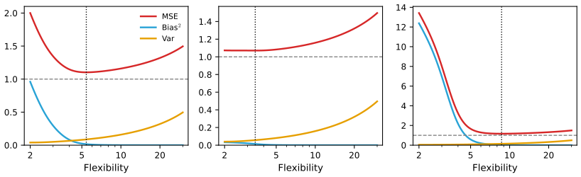
| Example | df | squared bias | variance | test MSE | training MSE |
|---|---|---|---|---|---|
| 1 (non-linear) | 2 / 5.4 / 25 | 0.960 / 0.015 / 0.000 | 0.040 / 0.087 / 0.406 | 2.000 / 1.103 / 1.406 | 1.871 / 0.883 / 0.390 |
| 2 (near linear) | 2 / 3.4 / 25 | 0.033 / 0.014 / 0.000 | 0.040 / 0.057 / 0.406 | 1.073 / 1.071 / 1.406 | 0.991 / 0.932 / 0.390 |
| 3 (far from linear) | 2 / 8.7 / 25 | 12.379 / 0.026 / 0.000 | 0.040 / 0.138 / 0.406 | 13.420 / 1.164 / 1.406 | 12.618 / 0.807 / 0.390 |
Two regularities in the table are worth noticing. The variance column does not depend on \(f\) at all (it is \(\sigma^2\) times an average of \(\|\bl(x_0)\|^2\), a property of the inputs and \(\lambda\)): at df 2 it is 0.040 in every example. And the training MSE at df 25 is the same, 0.390, in all three, because at that flexibility the bias has vanished and what remains, \(\sigma^2\tr(\bI-\bS)^2/n\), again depends only on \(\bS\).
p. 36 This is the bias-variance trade-off. It is easy to get low bias with high variance (a curve through every training point) or low variance with high bias (a horizontal line); the work is in finding methods for which both are low. In real problems \(f\) is unknown and the bias and variance cannot be computed, but the trade-off still governs what happens. If the true \(f\) is linear, linear regression has no bias and is hard to beat; if \(f\) is very non-linear and there is plenty of data, a flexible method can win, as in Figure 2.11.
2.2.3 The Classification Setting
p. 37 With a qualitative response the natural measure of accuracy is the error rate, the proportion of misclassified observations. On the training data it is the training error rate
\[ \frac1n\sum_{i=1}^n\I(y_i\ne\hat y_i), \tag{2.8} \]where \(\hat y_i\) is the predicted class and \(\I(y_i\ne\hat y_i)\) is 1 for a mistake and 0 otherwise; on test observations \((x_0,y_0)\) it is the test error rate
\[ \Ave\big(\I(y_0\ne\hat y_0)\big). \tag{2.9} \]As before, a good classifier is one with a small test error rate.
Result 2.5 (the Bayes classifier and the Bayes error rate) pp. 37–39, (2.10)–(2.11)
The expected test error rate is minimised by the Bayes classifier, which assigns a test observation with predictor \(x_0\) to the class \(j\) for which
\[ \Pr(Y=j\given X=x_0) \tag{2.10} \]is largest. With two classes, it predicts class 1 when \(\Pr(Y=1\given X=x_0)>0.5\). Its error rate, the Bayes error rate, is the smallest possible:
\[ 1-\E\Big(\max_j\Pr(Y=j\given X)\Big), \tag{2.11} \]where the expectation averages over \(X\). It is positive whenever the classes overlap, and plays the role that \(\Var(\varepsilon)\) plays in regression.
Filling the gap 2.7: why the Bayes classifier is optimal, and the error-rate formula p. 37, "the proof is outside of the scope of this book"
Optimality holds point by point: at each \(x\), choosing the most probable class gives the smallest probability of a mistake.
Derivation
Write \(p_j(x)=\Pr(Y=j\given X=x)\). A classifier \(C\) assigns class \(C(x)\) to the input \(x\). Conditionally on \(X=x\), it is correct with probability \(p_{C(x)}(x)\), so
\[ \Pr\big(C(X)\ne Y\given X=x\big)=1-p_{C(x)}(x)\ \ge\ 1-\max_jp_j(x), \]with equality exactly when \(C(x)\) is a most probable class. Averaging over \(X\) (the tower property) gives \(\Pr(C(X)\ne Y)\ge1-\E\max_jp_j(X)\), with equality for the Bayes classifier. That is optimality and (2.11) at once.
With known class densities. If class \(j\) has prior probability \(\pi_j\) and density \(f_j(x)\), Bayes' theorem gives \(p_j(x)=\pi_jf_j(x)/\sum_k\pi_kf_k(x)\). With two equally likely classes, \(1-\max_jp_j(x)=\min(f_1,f_2)/(f_1+f_2)\) and the marginal density of \(X\) is \((f_1+f_2)/2\), so
\[ \text{Bayes error rate}=\int\frac{\min\big(f_1(x),f_2(x)\big)}{f_1(x)+f_2(x)}\cdot\frac{f_1(x)+f_2(x)}{2}\,\d x=\frac12\int\min\big(f_1(x),f_2(x)\big)\,\d x, \]the area where the two densities overlap, halved. This is how the rate below is computed. (Confirmed numerically against a simulation of 400,000 points, which also shows that changing the Bayes decisions where \(0.4<p_j<0.6\) increases the error.) ∎
Deeper: Statistical Learning: Theory and Methods, Result 2.7 (the Bayes classifier with a general loss) and Filling the gap 2.4 (the Bayes boundary of a mixture).
See also (companion course): minimising the misclassification rate, with unequal losses in Section 1.5.2.
pp. 37–39 The simulated data of Figures 2.13–2.17. Again the book's simulation is not published, so here is one of the same kind: each class is an equal mixture of ten Gaussian clusters with covariance \(0.2\bI\); the ten blue centres are draws from \(\N((1,0)^\T,\bI)\) and the ten orange ones from \(\N((0,1)^\T,\bI)\). The centres were chosen (by the random seed) so that the Bayes error rate, 0.1331, is close to the book's 0.133. The training set has 100 points per class, the test set 2,500 per class.
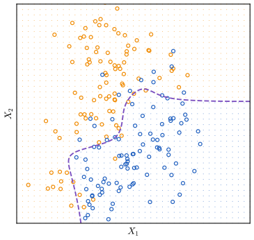
fig_2_13, bayes_prob, bayes_error. Reproduces James et al. (2021), Figure 2.13. Download: PDF · SVGFilling the gap 2.8: 0.133 or 0.1304? The Bayes error rate and its estimate on a test set pp. 39 and 41
The book quotes two numbers for the same simulation; they measure different things, and the difference is sampling error.
Derivation
The Bayes error rate (2.11) is a property of the population: 0.133 in the book, 0.1331 here (an integral, computed numerically). The error of the Bayes classifier on a finite test set of \(m\) independent points is an estimate of it: the number of mistakes is Binomial\((m,r)\), with standard error \(\sqrt{r(1-r)/m}\). For \(m=5{,}000\) and \(r=0.133\) that is 0.0048. The book's 0.1304 on its test set is 0.5 standard errors from 0.133; our 0.1228 is 2.1 standard errors below 0.1331, a somewhat unlucky but unremarkable test set. A consequence worth remembering: on a test set, a good classifier can appear to beat the Bayes rate, because both are measured with error. ∎
pp. 39–40 K-nearest neighbours. For real data \(\Pr(Y\given X)\) is unknown, so the Bayes classifier is an unattainable gold standard. Many methods estimate the conditional probabilities and then classify to the largest estimate; the simplest is K-nearest neighbours.
Definition 2.3 (the K-nearest-neighbour classifier) p. 39, (2.12)
Given a positive integer \(K\) and a test point \(x_0\), let \(\mathcal N_0\) be the \(K\) training points closest to \(x_0\) (in Euclidean distance). Estimate
\[ \Pr(Y=j\given X=x_0)\approx\frac1K\sum_{i\in\mathcal N_0}\I(y_i=j), \tag{2.12} \]and classify \(x_0\) to the class with the largest estimate. (With two classes and even \(K\) the vote can tie; the code here gives a tie to the class of the single nearest neighbour.)
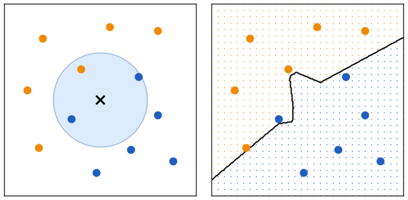
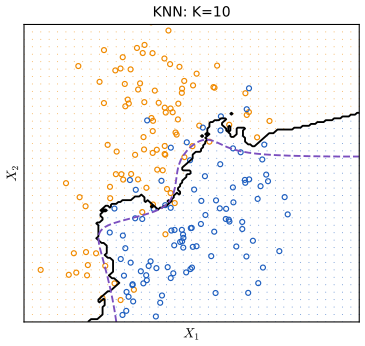
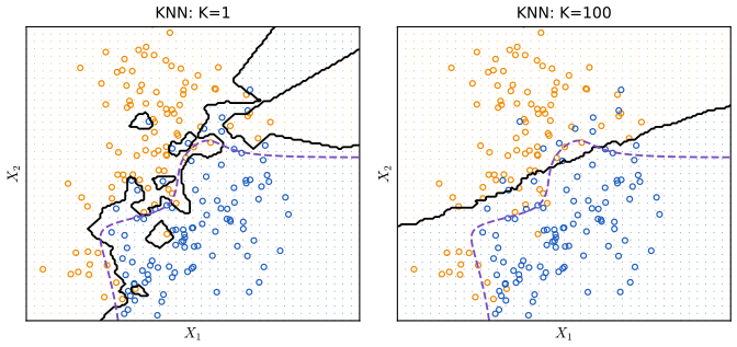
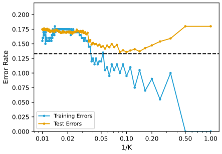
pp. 40–42 The choice of \(K\) matters a great deal. With \(K=1\) the boundary is overly flexible: low bias, very high variance. As \(K\) grows the boundary becomes smoother and, for large \(K\), close to linear: low variance, high bias. So \(1/K\) plays the role of flexibility, and the training and test error rates behave as in regression (Figure 2.17): the training error tends to fall as \(1/K\) grows and is zero at \(K=1\), while the test error is U-shaped, here with its minimum at \(K=10\).
Result 2.6 (properties of K-nearest neighbours)
(a) With \(K=1\) (and distinct training inputs) the training error rate is 0: each training point is its own nearest neighbour. (b) With \(K=n\) every point is assigned to the majority class of the training set. (c) If the \(K\) neighbours of \(x_0\) were drawn from a region where \(\Pr(Y=j\given X)\approx p\), the estimate (2.12) would be a binomial proportion with variance \(p(1-p)/K\): larger \(K\), smaller variance, but neighbours from further away and so more bias. (d) As \(n\to\infty\), the error rate of the 1-nearest-neighbour classifier with two classes tends to at most \(2r(1-r)\le2r\), where \(r\) is the Bayes error rate (Cover and Hart 1967).
Filling the gap 2.9: the four properties, and what they say here
Each property is short; together they explain the shape of Figure 2.17.
Derivation
(a) A training point is at distance 0 from itself and at positive distance from every other (distinct) input, so its single nearest neighbour is itself and the prediction is its own label. (With our tie rule \(K=2\) also has training error 0: the vote is either unanimous or tied, and a tie goes to the point itself.)
(b) With \(K=n\) the neighbourhood is the whole training set for every \(x_0\), so (2.12) is the overall class proportion.
(c) If the \(K\) labels are independent with \(\Pr(y_i=j)=p\), their sum is Binomial\((K,p)\) and the proportion has variance \(p(1-p)/K\). The neighbourhood that contains \(K\) points grows with \(K\), so the true probabilities inside it drift away from \(p_j(x_0)\): that drift is the bias.
(d) As \(n\to\infty\) the nearest neighbour \(x_{(1)}\) of \(x_0\) approaches \(x_0\), so its label is (almost) an independent draw from \(\Pr(Y\given X=x_0)\). With two classes and \(p=p_1(x_0)\), 1-NN errs when the test label and the neighbour's label differ: probability \(2p(1-p)\). With \(q=\min(p,1-p)\) the Bayes rule errs with probability \(q\), and \(2p(1-p)=2q(1-q)\). Averaging over \(x_0\) and using that \(q\mapsto2q(1-q)\) is concave (Jensen's inequality), the limit is at most \(2r(1-r)\). Here \(r=0.1331\) gives the bound 0.231; the 1-NN test error 0.180 is below it. ∎
Deeper: Statistical Learning: Theory and Methods, Section 2.3.2 (nearest neighbours as \(N/k\) effective parameters, Result 2.2), Result 13.7 (the Cover–Hart bound) and Result 7.2 (bias and variance of \(k\)-NN regression).
p. 42 In regression and in classification alike, choosing the right level of flexibility is critical, and the bias-variance trade-off makes it hard. Chapter 5 returns to this with methods (cross-validation, the bootstrap) that estimate the test error from the training data alone.
2.3 Lab: Introduction to R and Python
The two editions have different labs: the R edition introduces R (vectors, matrices, graphics, indexing, loading the Auto data, summaries), and the Python edition introduces Python, numpy, matplotlib and pandas, with extra sections on slices, Boolean indexing, data-frame selection, loops and string formatting. Here the two are merged: every step is written in both languages, R on the left and Python on the right (one above the other on a phone), with the printed output underneath. The code is that of the course files ch02_lab.R and ch02_lab.py, which also contain the solutions of the applied exercises; each block starts in the files with section("...") under the same title. Where the languages behave differently, an orange note says so.
2.3.1 Getting Started
R edition p. 42; Python edition p. 40 R is free from cran.r-project.org and is usually run in an editor such as RStudio. Python 3 with Jupyter notebooks is the setting of the Python edition (installable, for example, with the Anaconda distribution). The Python edition installs a companion package, ISLP, for its data sets and helper functions; this course does not use it: the data are read from the CSV files on the book's website with pandas, and every method is written with numpy, pandas, statsmodels and scikit-learn. Both lab files run from the command line (Rscript ch02_lab.R, python3 ch02_lab.py); they look for the data in a folder isl-data next to them (or in the folder named by the environment variable ISL_DATA) and write their figures to img/ch02/. Help is ?funcname in R, help(fun) or fun? (in Jupyter) in Python.
2.3.2 Basic Commands
Functions are called as fun(input1, input2) in both languages. In R, c() concatenates numbers into a vector and <- (or =) assigns. In Python, square brackets make a list, and print() displays results (in a script nothing is printed automatically, whereas R prints any top-level value).
x <- c(1, 3, 2, 5)
x
x = c(1, 6, 2)          # = also assigns, but <- is the usual R style
x
y = c(1, 4, 3)
length(x)
length(y)
[1] 1 3 2 5
[1] 1 6 2
[1] 3
[1] 3print('fit a model with', 11, 'variables')
print(3 + 5)
print("hello" + " " + "world")
x = [3, 4, 5]
print(x)
y = [4, 9, 7]
print(len(x), len(y))fit a model with 11 variables
8
hello world
[3, 4, 5]
3 3Adding two vectors is where the languages first part company.
x + y # elementwise: R vectors are numeric by nature[1] 2 10 5print(x + y) # lists are joined end to end, not added
x = np.array([3, 4, 5])
y = np.array([4, 9, 7])
print(x + y) # numpy arrays add elementwise[3, 4, 5, 4, 9, 7]
[ 7 13 12]R and Python differ: R vectors are numeric, and + adds them element by element. Python lists hold arbitrary objects, and + joins them end to end (as it joins strings); elementwise arithmetic needs numpy arrays.
ls()
rm(x, y)
exists("x")
[1] "DATA" "IMG" "open_png" "open_svg" "report" "section" "x"
[8] "y"
[1] FALSEprint([name for name in ("x", "y") if name in globals()])
del x, y
print("x" in globals())['x', 'y']
FalseR's ls() lists everything defined so far (here including the small helpers at the top of the lab file); rm() deletes objects. Python's del does the same; globals() holds the names.
2.3.3 Vectors, Matrices and Numerical Arrays
R edition p. 43; Python edition pp. 42–48 In R, matrix() builds a matrix from a vector, a number of rows and a number of columns. In Python the numpy package (imported as np) provides arrays: two-dimensional arrays play the role of matrices. Arrays have attributes (x.ndim, x.shape, x.dtype) and methods (x.sum()).
x <- matrix(data = c(1, 2, 3, 4), nrow = 2, ncol = 2)
x
dim(x)
typeof(x)
[,1] [,2]
[1,] 1 3
[2,] 2 4
[1] 2 2
[1] "double"x = np.array([[1, 2], [3, 4]])
print(x)
print(x.ndim, x.shape, x.dtype)
print(np.array([[1, 2], [3.0, 4]]).dtype)
print(np.array([[1, 2], [3, 4]], float).dtype)
print(x.sum(), np.sum(x))[[1 2]
[3 4]]
2 (2, 2) int64
float64
float64
10 10matrix(c(1, 2, 3, 4), 2, 2, byrow = TRUE) # R fills by column unless byrow = TRUE
v <- 1:6
dim(v) <- c(2, 3) # reshape in place: still column-major
v [,1] [,2]
[1,] 1 2
[2,] 3 4
[,1] [,2] [,3]
[1,] 1 3 5
[2,] 2 4 6x = np.array([1, 2, 3, 4, 5, 6])
x_reshape = x.reshape((2, 3)) # numpy fills by row (row-major order)
print(x_reshape)
print(x.reshape((2, 3), order="F")) # column-major order, as R's matrix()
print(x_reshape[0, 0], x_reshape[1, 2], x[2])[[1 2 3]
[4 5 6]]
[[1 3 5]
[2 4 6]]
1 6 3R and Python differ: R fills a matrix column by column (column-major order) unless byrow = TRUE; numpy fills row by row (row-major order) unless order="F". R counts positions from 1, Python from 0: R's x[1, 1] is Python's x[0, 0].
w <- v                  # R copies on modification: changing w leaves v alone
w[1, 1] <- 5
v[1, 1]
w[1, 1]
[1] 1
[1] 5x_reshape[0, 0] = 5 # x_reshape is a view of x: both change
print(x_reshape)
print(x)
my_tuple = (3, 4, 5)
try:
my_tuple[0] = 2
except TypeError as err:
print("TypeError:", err)
print(x_reshape.shape, x_reshape.ndim)
print(x_reshape.T)[[5 2 3]
[4 5 6]]
[5 2 3 4 5 6]
TypeError: 'tuple' object does not support item assignment
(2, 3) 2
[[5 4]
[2 5]
[3 6]]R and Python differ: in Python, x.reshape(...) returns a view of the same memory, so changing x_reshape changed x too; use .copy() when that is not wanted. R copies on modification, so w[1, 1] <- 5 leaves v unchanged. Python tuples, unlike lists and arrays, cannot be modified at all.
sqrt(x)
x^2
x^0.5
[,1] [,2]
[1,] 1.000000 1.732051
[2,] 1.414214 2.000000
[,1] [,2]
[1,] 1 9
[2,] 4 16
[,1] [,2]
[1,] 1.000000 1.732051
[2,] 1.414214 2.000000print(np.sqrt(x))
print(x**2)
print(x**0.5)[2.23606798 1.41421356 1.73205081 2. 2.23606798 2.44948974]
[25 4 9 16 25 36]
[2.23606798 1.41421356 1.73205081 2. 2.23606798 2.44948974]Random numbers. R's rnorm(n, mean, sd) and numpy's rng.normal(loc, scale, size) generate normal variables. The R lab adds noise with standard deviation 0.1 to x (correlation near 1); the Python lab adds noise with standard deviation 1 (correlation about 0.7).
set.seed(1)
x <- rnorm(50)
y <- x + rnorm(50, mean = 50, sd = 0.1)
cor(x, y)
[1] 0.9932279rng = np.random.default_rng(1)
x = rng.normal(size=50)
y = x + rng.normal(loc=50, scale=1, size=50)
print(np.corrcoef(x, y))[[1. 0.71706035]
[0.71706035 1. ]]To make random results reproducible, R sets a global seed with set.seed(); numpy creates a generator object with np.random.default_rng(seed) and draws from it. With the books' seeds the output is exactly what the two editions print: R's set.seed(1303) starts −1.1440, 1.3421, 2.1854, ..., and numpy's generator with seed 1303 gives 4.09, −1.07.
set.seed(1303)
round(rnorm(50), 4)[1:7]
set.seed(1303)
round(rnorm(50), 4)[1:7]  # the same numbers again
[1] -1.1440 1.3421 2.1854 0.5364 0.0632 0.5022 -0.0004
[1] -1.1440 1.3421 2.1854 0.5364 0.0632 0.5022 -0.0004rng = np.random.default_rng(1303)
print(rng.normal(scale=5, size=2))
rng2 = np.random.default_rng(1303)
print(rng2.normal(scale=5, size=2)) # the same numbers again[ 4.09482632 -1.07485605]
[ 4.09482632 -1.07485605]R and Python differ: the two languages use different random number generators, so the same seed gives different numbers in R and Python. Results that depend on random draws (here, and in later chapters random splits and simulations) agree between the two only in distribution, not digit by digit.
set.seed(3)
y <- rnorm(100)
mean(y)
var(y)                  # divisor n - 1
sqrt(var(y))
sd(y)
report("variance with divisor n", mean((y - mean(y))^2))
[1] 0.01103557
[1] 0.7328675
[1] 0.8560768
[1] 0.8560768
variance with divisor n: 0.7255rng = np.random.default_rng(3)
y = rng.standard_normal(10)
print(np.mean(y), y.mean())
print(np.var(y), y.var(), np.mean((y - y.mean())**2)) # divisor n
print(np.sqrt(np.var(y)), np.std(y))
report("variance with divisor n - 1", np.var(y, ddof=1))-0.1126795190952861 -0.1126795190952861
2.7243406406465125 2.7243406406465125 2.7243406406465125
1.6505576756498128 1.6505576756498128
variance with divisor n - 1: 3.0270R and Python differ: R's var() and sd() divide by \(n-1\) (the unbiased variance estimate); np.var() and np.std() divide by \(n\) unless ddof=1 is given. (pandas methods .var() and .std() divide by \(n-1\), like R.) The book's Python output, mean \(-0.11\) and variance 2.72 for ten standard normal draws, is reproduced exactly; the variance is large for a sample of ten, but that is the draw.
X <- matrix(rnorm(30), 10, 3)
colMeans(X)
apply(X, 2, mean)       # the same, by applying mean() to each column
[1] 0.16010533 -0.03431017 -0.20283210
[1] 0.16010533 -0.03431017 -0.20283210X = rng.standard_normal((10, 3))
print(X.mean(axis=0))
print(X.mean(0))[ 0.15030588 0.14030961 -0.34238602]
[ 0.15030588 0.14030961 -0.34238602]In numpy, axis=0 means "along the rows", that is one result per column; R has colMeans() and the general apply(X, 2, f).
2.3.4 Graphics
R edition pp. 45–47; Python edition pp. 48–50 R draws with plot() on the current device, and saves to a file by opening a file device (pdf(), jpeg(), ...) and closing it with dev.off(). Python uses matplotlib: subplots() returns a figure (the whole canvas) and one or more axes (the plots), and every change is a method call on an axes object; fig.savefig() writes a file.
x <- rnorm(100)
y <- rnorm(100)
plot(x, y, xlab = "this is the x-axis", ylab = "this is the y-axis", main = "Plot of X vs Y")
(no printed output)fig, ax = subplots(figsize=(8, 8))
x = rng.standard_normal(100)
y = rng.standard_normal(100)
ax.plot(x, y, 'o')
ax.scatter(x, y, marker='o')
ax.set_xlabel("this is the x-axis")
ax.set_ylabel("this is the y-axis")
ax.set_title("Plot of X vs Y")
fig.set_size_inches(12, 3)
close(fig)(no printed output)pdf(file.path(IMG, "lab-r-scatter.pdf"), width = 9, height = 4)
par(mfrow = c(2, 3)) # a 2 x 3 grid, filled row by row
plot(x, y, col = "green")
plot(x, y, pch = 3)
invisible(dev.off())(no printed output)fig, axes = subplots(nrows=2, ncols=3, figsize=(15, 5))
axes[0, 1].plot(x, y, 'o')
axes[1, 2].scatter(x, y, marker='+')
fig.savefig(os.path.join(IMG, "lab-py-scatter.pdf"))
axes[0, 1].set_xlim([-1, 1])
close(fig)(no printed output)Sequences: R's seq(a, b) and a:b include both ends; numpy's np.arange(a, b) stops before b, while np.linspace(a, b, n) gives \(n\) equally spaced points including both ends (like R's seq(a, b, length = n)).
seq(1, 10)
1:10
seq(0, 1, length = 11)
x <- seq(-pi, pi, length = 50)
[1] 1 2 3 4 5 6 7 8 9 10
[1] 1 2 3 4 5 6 7 8 9 10
[1] 0.0 0.1 0.2 0.3 0.4 0.5 0.6 0.7 0.8 0.9 1.0print(np.linspace(0, 10, 11))
print(np.arange(0, 10)) # stops before 10
print(np.linspace(0, 1, 11))
x = np.linspace(-np.pi, np.pi, 50)[ 0. 1. 2. 3. 4. 5. 6. 7. 8. 9. 10.]
[0 1 2 3 4 5 6 7 8 9]
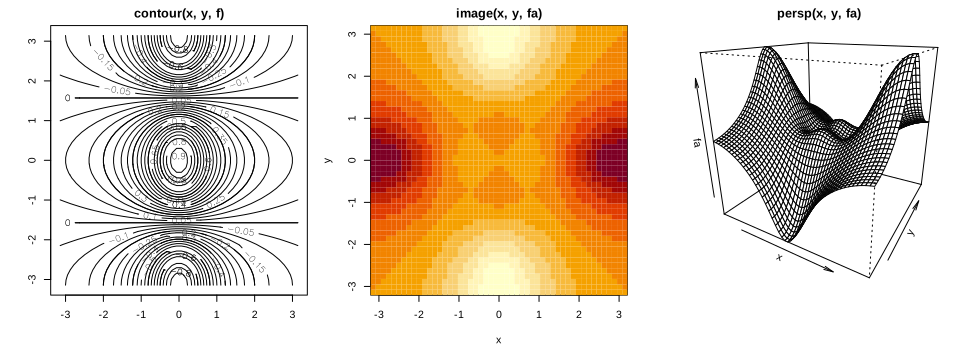
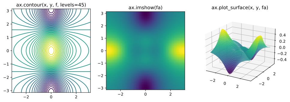
[0. 0.1 0.2 0.3 0.4 0.5 0.6 0.7 0.8 0.9 1. ]A contour plot shows a function of two variables through its level curves; a heatmap (image() in R, ax.imshow() in Python) shows it by colour; a perspective plot draws the surface in three dimensions. The function is \(f(x,y)=\cos(y)/(1+x^2)\) on a \(50\times50\) grid, and fa its antisymmetric part \(\tfrac12\{f(x,y)-f(y,x)\}\).
y <- x
f <- outer(x, y, function(x, y) cos(y) / (1 + x^2))   # f[i, j] is the value at (x[i], y[j])
fa <- (f - t(f)) / 2                                  # the antisymmetric part
report("f at (x[2], y[5])", f[2, 5])
report("largest |fa|", max(abs(fa)))
open_svg("lab-r-contour", 10, 3.6)
par(mfrow = c(1, 3), mar = c(4, 4, 2, 1))
contour(x, y, f, main = "contour(x, y, f)")
contour(x, y, f, nlevels = 45, add = TRUE)
image(x, y, fa, main = "image(x, y, fa)")
persp(x, y, fa, theta = 30, phi = 20, main = "persp(x, y, fa)")
invisible(dev.off())
f at (x[2], y[5]): -0.0864
largest |fa|: 0.5439y = x
f = np.multiply.outer(np.cos(y), 1 / (1 + x**2)) # f[j, i] is the value at (x[i], y[j])
fa = (f - f.T) / 2 # the antisymmetric part
report("f at (x[2], y[5])", f[4, 1])
report("largest |fa|", np.max(np.abs(fa)))
fig = figure(figsize=(12, 3.8))
ax1, ax2 = fig.add_subplot(1, 3, 1), fig.add_subplot(1, 3, 2)
ax3 = fig.add_subplot(1, 3, 3, projection="3d")
ax1.contour(x, y, f, levels=45)
ax1.set_title("ax.contour(x, y, f, levels=45)")
ax2.imshow(fa, origin="lower", extent=(-np.pi, np.pi, -np.pi, np.pi))
ax2.set_title("ax.imshow(fa)")
X1, Y1 = np.meshgrid(x, y)
ax3.plot_surface(X1, Y1, fa, cmap="viridis")
ax3.view_init(elev=20, azim=-60)
ax3.set_title("ax.plot_surface(x, y, fa)")
save(fig, "lab-py-contour")f at (x[2], y[5]): -0.0864
largest |fa|: 0.5439R and Python differ: R's contour(x, y, z) expects z[i, j] to be the value at \((x_i,y_j)\), so outer(x, y, ...) puts \(x\) along the rows. Matplotlib's contour(x, y, Z) expects Z[j, i] at \((x_i,y_j)\), rows along \(y\), which is why the Python edition builds np.multiply.outer(np.cos(y), 1 / (1 + x**2)). The same value therefore sits at f[2, 5] in R and f[4, 1] in Python (both print \(-0.0864\)), and the antisymmetric parts are the same surface. Colours differ too: R's default image() palette is dark for large values, matplotlib's viridis is yellow for large values.
2.3.5 Sequences, Slices and Indexing Data
R edition pp. 47–48; Python edition pp. 51–54 Python's slice a:b takes positions \(a,a+1,\dots,b-1\) (counting from 0); it works on strings, lists, tuples and arrays, and a:b:s takes every \(s\)-th position.
substr("hello world", 4, 6)        # characters 4 to 6 (both ends included)
(0:9)[4:6]                         # R positions start at 1
[1] "lo "
[1] 3 4 5print("hello world"[3:6]) # positions 3, 4, 5 (the end is excluded)
print("hello world"[slice(3, 6)])
print(np.arange(10)[3:6])lo
lo
[3 4 5]A <- matrix(1:16, 4, 4)
A
A[2, 3]
B <- matrix(0:15, 4, 4, byrow = TRUE) # the array np.arange(16).reshape(4, 4) of the Python lab
B[2, 3] [,1] [,2] [,3] [,4]
[1,] 1 5 9 13
[2,] 2 6 10 14
[3,] 3 7 11 15
[4,] 4 8 12 16
[1] 10
[1] 6A = np.array(np.arange(16)).reshape((4, 4))
print(A)
print(A[1, 2])
A_R = np.arange(1, 17).reshape((4, 4), order="F") # the matrix(1:16, 4, 4) of the R lab
print(A_R[1, 2])[[ 0 1 2 3]
[ 4 5 6 7]
[ 8 9 10 11]
[12 13 14 15]]
6
10R and Python differ: the "same" \(4\times4\) matrix of 16 numbers is different in the two labs: R's matrix(1:16, 4, 4) holds 1 to 16 down the columns, numpy's np.arange(16).reshape((4, 4)) holds 0 to 15 along the rows. Hence A[2, 3] is 10 in R while A[1, 2] (the same position) is 6 in Python. The lines B and A_R rebuild each language's matrix in the other.
A[c(1, 3), c(2, 4)]
A[1:3, 2:4]
A[1:2, ]
A[, 1:2]
A[1, ]
A[-c(1, 3), ]
A[-c(1, 3), -c(1, 3, 4)]
dim(A)
[,1] [,2]
[1,] 5 13
[2,] 7 15
[,1] [,2] [,3]
[1,] 5 9 13
[2,] 6 10 14
[3,] 7 11 15
[,1] [,2] [,3] [,4]
[1,] 1 5 9 13
[2,] 2 6 10 14
[,1] [,2]
[1,] 1 5
[2,] 2 6
[3,] 3 7
[4,] 4 8
[1] 1 5 9 13
[,1] [,2] [,3] [,4]
[1,] 2 6 10 14
[2,] 4 8 12 16
[1] 6 8
... (1 more lines)print(A[[1, 3]])
print(A[:, [0, 2]])
print(A[[1, 3], [0, 2]]) # pairs (1, 0) and (3, 2): not a submatrix
print(A[[1, 3]][:, [0, 2]])
print(A[np.ix_([1, 3], [0, 2, 3])])
print(A[1:4:2, 0:3:2])
print(A.shape)[[ 4 5 6 7]
[12 13 14 15]]
[[ 0 2]
[ 4 6]
[ 8 10]
[12 14]]
[ 4 14]
[[ 4 6]
[12 14]]
[[ 4 6 7]
[12 14 15]]
[[ 4 6]
[12 14]]
(4, 4)R and Python differ: in R, A[c(1, 3), c(2, 4)] is the submatrix of rows 1, 3 and columns 2, 4. In numpy, A[[1, 3], [0, 2]] is not: two index lists are read as pairs \((1,0)\) and \((3,2)\), giving two elements. The submatrix needs np.ix_(), two steps (A[[1, 3]][:, [0, 2]]) or slices. R's negative indices (A[-c(1, 3), ]) drop rows; Python's negative indices count from the end.
keep_rows <- c(FALSE, TRUE, FALSE, TRUE)
A[keep_rows, ]
A[c(1, 2, 1, 2), ]                     # integers select (and repeat) rows
A[keep_rows, c(TRUE, FALSE, TRUE, TRUE)]
[,1] [,2] [,3] [,4]
[1,] 2 6 10 14
[2,] 4 8 12 16
[,1] [,2] [,3] [,4]
[1,] 1 5 9 13
[2,] 2 6 10 14
[3,] 1 5 9 13
[4,] 2 6 10 14
[,1] [,2] [,3]
[1,] 2 10 14
[2,] 4 12 16keep_rows = np.zeros(A.shape[0], bool)
keep_rows[[1, 3]] = True
print(keep_rows, np.all(keep_rows == np.array([0, 1, 0, 1])))
print(A[np.array([0, 1, 0, 1])]) # integers select (and repeat) rows
print(A[keep_rows])
keep_cols = np.zeros(A.shape[1], bool)
keep_cols[[0, 2, 3]] = True
print(A[np.ix_(keep_rows, keep_cols)])
print(A[np.ix_([1, 3], keep_cols)])[False True False True] True
[[0 1 2 3]
[4 5 6 7]
[0 1 2 3]
[4 5 6 7]]
[[ 4 5 6 7]
[12 13 14 15]]
[[ 4 6 7]
[12 14 15]]
[[ 4 6 7]
[12 14 15]]In both languages a logical (Boolean) vector selects the positions where it is true, while an integer vector selects (and can repeat) positions, even though c(FALSE, TRUE, FALSE, TRUE) and c(0, 1, 0, 1) compare as equal.
2.3.6 Loading Data
R edition pp. 48–50; Python edition pp. 55–56 The Auto data (gas mileage, engine and other characteristics of 397 cars) are on the book's website as a whitespace-separated text file Auto.data and as Auto.csv. Two things can go wrong when reading them: the first line holds the variable names, not data; and missing horsepower values are coded ?, which turns the whole column into text.
Auto <- read.table(file.path(DATA, "Auto.data"))
head(Auto, 3)                           # wrong: the header line was read as data
Auto <- read.table(file.path(DATA, "Auto.data"), header = TRUE, na.strings = "?", stringsAsFactors = TRUE)
Auto <- read.csv(file.path(DATA, "Auto.csv"), na.strings = "?", stringsAsFactors = TRUE)
dim(Auto)
Auto[1:4, ]
report("horsepower total (missing values skipped)", sum(Auto$horsepower, na.rm = TRUE))
V1 V2 V3 V4 V5 V6 V7 V8
1 mpg cylinders displacement horsepower weight acceleration year origin
2 18.0 8 307.0 130.0 3504. 12.0 70 1
3 15.0 8 350.0 165.0 3693. 11.5 70 1
V9
1 name
2 chevrolet chevelle malibu
3 buick skylark 320
[1] 397 9
mpg cylinders displacement horsepower weight acceleration year origin
1 18 8 307 130 3504 12.0 70 1
2 15 8 350 165 3693 11.5 70 1
3 18 8 318 150 3436 11.0 70 1
4 16 8 304 150 3433 12.0 70 1
name
1 chevrolet chevelle malibu
... (4 more lines)Auto = pd.read_csv(os.path.join(DATA, "Auto.csv"))
print(Auto["horsepower"].dtype) # object: the column holds text
print(np.unique(Auto["horsepower"])[-3:])
Auto = pd.read_csv(os.path.join(DATA, "Auto.data"), na_values=["?"], sep=r"\s+")
print(Auto.shape)
print(Auto[:4])
report("horsepower total (missing values skipped)", Auto["horsepower"].sum())object
['97' '98' '?']
(397, 9)
mpg cylinders displacement ... year origin name
0 18.0 8 307.0 ... 70 1 chevrolet chevelle malibu
1 15.0 8 350.0 ... 70 1 buick skylark 320
2 18.0 8 318.0 ... 70 1 plymouth satellite
3 16.0 8 304.0 ... 70 1 amc rebel sst
[4 rows x 9 columns]
horsepower total (missing values skipped): 40952R and Python differ: R's read.table() assumes there is no header line (hence header = TRUE), while pandas' read_csv() assumes there is one. The missing-value code is na.strings = "?" in R and na_values=["?"] in pandas. The Python edition reads Auto.data with delim_whitespace=True, which pandas 2.2 deprecates; sep=r"\s+" does the same. Both versions find 397 rows and 9 columns, and a horsepower total of 40,952 over the 392 non-missing values, as printed in the Python edition.
colSums(is.na(Auto))
Auto <- na.omit(Auto)
dim(Auto)
names(Auto)
mpg cylinders displacement horsepower weight acceleration
0 0 0 5 0 0
year origin name
0 0 0
[1] 392 9
[1] "mpg" "cylinders" "displacement" "horsepower" "weight"
[6] "acceleration" "year" "origin" "name"print(Auto.isna().sum())
Auto_new = Auto.dropna()
Auto = Auto_new # overwrite the previous value
print(Auto.shape)
print(list(Auto.columns))mpg 0
cylinders 0
displacement 0
horsepower 5
weight 0
acceleration 0
year 0
origin 0
name 0
dtype: int64
(392, 9)
['mpg', 'cylinders', 'displacement', 'horsepower', 'weight', 'acceleration', 'year', 'origin', 'name']Five cars have no horsepower; dropping them (na.omit() in R, .dropna() in pandas) leaves 392 rows, the version of Auto used in the rest of the book.
2.3.7 Selecting Rows and Columns
Python edition pp. 56–59 A data frame is indexed by rows and columns, by position, by name or by a logical condition. In pandas, [] with a slice or Boolean array selects rows and with a list of names selects columns; .loc[] selects by labels or Booleans and .iloc[] by integer positions.
Auto[1:3, ]
idx_80 <- Auto$year > 80
report("cars with year > 80", sum(idx_80))
head(Auto[, c("mpg", "horsepower")])
mpg cylinders displacement horsepower weight acceleration year origin
1 18 8 307 130 3504 12.0 70 1
2 15 8 350 165 3693 11.5 70 1
3 18 8 318 150 3436 11.0 70 1
name
1 chevrolet chevelle malibu
2 buick skylark 320
3 plymouth satellite
cars with year > 80: 58
mpg horsepower
1 18 130
2 15 165
3 18 150
4 16 150
5 17 140
6 15 198print(Auto[:3])
idx_80 = Auto["year"] > 80
report("cars with year > 80", idx_80.sum())
print(Auto[["mpg", "horsepower"]].head())
print(Auto.index[:5], len(Auto.index)) mpg cylinders displacement ... year origin name
0 18.0 8 307.0 ... 70 1 chevrolet chevelle malibu
1 15.0 8 350.0 ... 70 1 buick skylark 320
2 18.0 8 318.0 ... 70 1 plymouth satellite
[3 rows x 9 columns]
cars with year > 80: 58
mpg horsepower
0 18.0 130.0
1 15.0 165.0
2 18.0 150.0
3 16.0 150.0
4 17.0 140.0
Index([0, 1, 2, 3, 4], dtype='int64') 392Auto[Auto$name %in% c("amc rebel sst", "ford torino"), c("mpg", "displacement", "horsepower")]
Auto[Auto$name == "ford galaxie 500", c("mpg", "origin")] mpg displacement horsepower
4 16 304 150
5 17 302 140
mpg origin
6 15 1
41 14 1
66 14 1Auto_re = Auto.set_index("name")
rows = ["amc rebel sst", "ford torino"]
print(Auto_re.loc[rows, ["mpg", "displacement", "horsepower"]])
print(Auto_re.iloc[[3, 4], [0, 2, 3]])
print(Auto_re.loc["ford galaxie 500", ["mpg", "origin"]]) mpg displacement horsepower
name
amc rebel sst 16.0 304.0 150.0
ford torino 17.0 302.0 140.0
mpg displacement horsepower
name
amc rebel sst 16.0 304.0 150.0
ford torino 17.0 302.0 140.0
mpg origin
name
ford galaxie 500 15.0 1
ford galaxie 500 14.0 1
ford galaxie 500 14.0 1R and Python differ: the Python edition makes the car names the row index (set_index("name")) and looks rows up by name; an index may repeat (there are three ford galaxie 500). R's row names must be unique, so the R version keeps name as a column and selects with a condition on it.
sel1 <- subset(Auto, year > 80, select = c(weight, origin))
sel2 <- subset(Auto, year > 80 & mpg > 30, select = c(weight, origin))
sel3 <- subset(Auto, displacement < 300 & grepl("ford|datsun", name), select = c(weight, origin))
report("rows selected (year > 80; and mpg > 30; ford or datsun with displacement < 300)",
       c(nrow(sel1), nrow(sel2), nrow(sel3)))
head(sel3, 4)
rows selected (year > 80; and mpg > 30; ford or datsun with displacement < 300): 58 34 51
weight origin
18 2587 1
19 2130 3
30 2130 3
37 3302 1sel1 = Auto_re.loc[idx_80.to_numpy(), ["weight", "origin"]]
sel2 = Auto_re.loc[lambda df: (df["year"] > 80) & (df["mpg"] > 30), ["weight", "origin"]]
sel3 = Auto_re.loc[lambda df: (df["displacement"] < 300)
& (df.index.str.contains("ford") | df.index.str.contains("datsun")),
["weight", "origin"]]
report("rows selected (year > 80; and mpg > 30; ford or datsun with displacement < 300)",
[len(sel1), len(sel2), len(sel3)])
print(sel3.head(4))rows selected (year > 80; and mpg > 30; ford or datsun with displacement < 300): 58 34 51
weight origin
name
ford maverick 2587.0 1
datsun pl510 2130.0 3
datsun pl510 2130.0 3
ford torino 500 3302.0 1Both versions select the same rows: 58 cars from after 1980, 34 of them with more than 30 miles per gallon, and 51 Fords or Datsuns with displacement below 300. In R, subset() and grepl() play the roles of a lambda inside .loc[] and str.contains().
2.3.8 For Loops and String Formatting
Python edition pp. 59–61 A for loop repeats a block for each value of a sequence. In Python the block is marked by indentation, in R by braces (or a single statement); Python's zip() walks through two lists in step, which R does with an index over seq_along().
total <- 0
for (value in c(3, 2, 19)) total <- total + value
cat("Total is:", total, "\n")
total <- 0
for (value in c(2, 3, 19)) for (weight in c(3, 2, 1)) total <- total + value * weight
cat("Total is:", total, "\n")
values <- c(2, 3, 19)
weights <- c(0.2, 0.3, 0.5)
total <- 0
for (i in seq_along(values)) total <- total + weights[i] * values[i]
cat("Weighted average is:", total, "\n")
Total is: 24
Total is: 144
Weighted average is: 10.8total = 0
for value in [3, 2, 19]:
total += value
print('Total is: {0}'.format(total))
total = 0
for value in [2, 3, 19]:
for weight in [3, 2, 1]:
total += value * weight
print('Total is: {0}'.format(total))
total = 0
for value, weight in zip([2, 3, 19], [0.2, 0.3, 0.5]):
total += weight * value
print('Weighted average is: {0}'.format(total))Total is: 24
Total is: 144
Weighted average is: 10.8set.seed(1)
A <- matrix(rnorm(127 * 5), 127, 5)
M <- matrix(sample(c(0, NA), 127 * 5, replace = TRUE, prob = c(0.8, 0.2)), 127, 5)
D <- as.data.frame(A + M)
names(D) <- c("food", "bar", "pickle", "snack", "popcorn")
for (col in names(D)) cat(sprintf('Column "%s" has %.2f%% missing values\n', col, 100 * mean(is.na(D[[col]]))))Column "food" has 17.32% missing values
Column "bar" has 24.41% missing values
Column "pickle" has 26.77% missing values
Column "snack" has 22.05% missing values
Column "popcorn" has 19.69% missing valuesrng = np.random.default_rng(1)
A = rng.standard_normal((127, 5))
M = rng.choice([0, np.nan], p=[0.8, 0.2], size=A.shape)
A += M
D = pd.DataFrame(A, columns=["food", "bar", "pickle", "snack", "popcorn"])
print(D[:3])
for col in D.columns:
template = 'Column "{0}" has {1:.2%} missing values'
print(template.format(col, np.isnan(D[col]).mean())) food bar pickle snack popcorn
0 0.345584 0.821618 0.330437 -1.303157 NaN
1 NaN -0.536953 0.581118 0.364572 0.294132
2 NaN 0.546713 NaN -0.162910 -0.482119
Column "food" has 16.54% missing values
Column "bar" has 25.98% missing values
Column "pickle" has 29.13% missing values
Column "snack" has 21.26% missing values
Column "popcorn" has 22.83% missing valuesR and Python differ: Python formats with '{0} ... {1:.2%}'.format(...) (or f-strings), R with sprintf() and C-style codes such as %.2f. The Python numbers (16.54% missing for food, and so on) are exactly those printed in the Python edition; the R numbers differ because the random generators differ.
2.3.9 Additional Graphical and Numerical Summaries
R edition pp. 50–52; Python edition pp. 61–62 Neither language finds a column of a data frame by its bare name: R needs Auto$horsepower (or attach(Auto), which the R edition uses but which is best avoided because it hides where variables come from), Python needs Auto["horsepower"] or Auto.horsepower, or a plotting method of the data frame itself.
plot(Auto$horsepower, Auto$mpg, xlab = "horsepower", ylab = "mpg", main = "Horsepower vs. MPG")
report("correlation of horsepower and mpg", cor(Auto$horsepower, Auto$mpg))
correlation of horsepower and mpg: -0.7784ax = Auto.plot.scatter("horsepower", "mpg")
ax.set_title("Horsepower vs. MPG")
close(ax.figure)
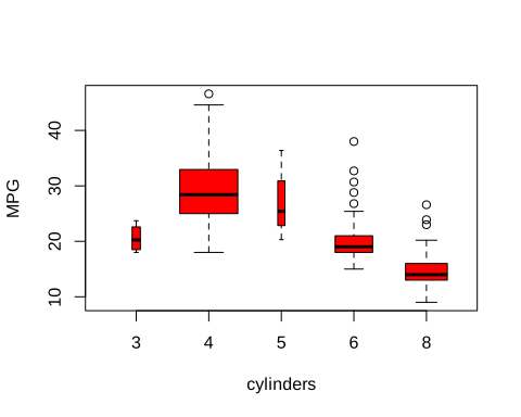
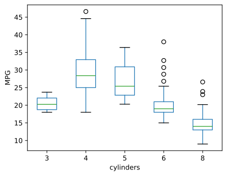
report("correlation of horsepower and mpg", Auto["horsepower"].corr(Auto["mpg"]))correlation of horsepower and mpg: -0.7784cylinders takes only five values, so it is better treated as qualitative: as.factor() in R, the category type in pandas. Plotting a quantitative variable against a factor then gives side-by-side boxplots.
Auto$cylinders <- as.factor(Auto$cylinders)
table(Auto$cylinders)
report("median mpg for 3, 4, 5, 6, 8 cylinders", tapply(Auto$mpg, Auto$cylinders, median))
open_svg("lab-r-boxplot", 5, 4)
plot(Auto$cylinders, Auto$mpg, col = "red", varwidth = TRUE, xlab = "cylinders", ylab = "MPG")
invisible(dev.off())
3 4 5 6 8
4 199 3 83 103
median mpg for 3, 4, 5, 6, 8 cylinders: 20.2500 28.4000 25.4000 19.0000 14.0000Auto.cylinders = pd.Series(Auto.cylinders, dtype="category")
print(Auto.cylinders.value_counts().sort_index())
report("median mpg for 3, 4, 5, 6, 8 cylinders", Auto.groupby("cylinders", observed=True)["mpg"].median())
fig, ax = subplots(figsize=(5, 4))
Auto.boxplot("mpg", by="cylinders", ax=ax, grid=False)
fig.suptitle("") # pandas adds a "grouped by" title; drop it
ax.set_title("")
ax.set_xlabel("cylinders")
ax.set_ylabel("MPG")
save(fig, "lab-py-boxplot")cylinders
3 4
4 199
5 3
6 83
8 103
Name: count, dtype: int64
median mpg for 3, 4, 5, 6, 8 cylinders: 20.2500 28.4000 25.4000 19.0000 14.0000h <- hist(Auto$mpg, breaks = 15, plot = FALSE)
report("histogram break points", h$breaks)
open_svg("lab-r-hist", 5, 4)
hist(Auto$mpg, col = 2, breaks = 15, main = "Histogram of mpg", xlab = "mpg")
invisible(dev.off())histogram break points: 8 10 12 14 16 18 20 22 24 26 28 30 32 34 36 38 40 42 44 46 48counts, edges = np.histogram(Auto["mpg"], bins=12)
report("histogram break points", edges)
fig, ax = subplots(figsize=(5, 4))
Auto.hist("mpg", color="red", bins=12, ax=ax, grid=False)
save(fig, "lab-py-hist")histogram break points: 9.0000 12.1333 15.2667 18.4000 21.5333 24.6667 27.8000 30.9333 34.0667 37.2000 40.3333 43.4667 46.6000R and Python differ: R's breaks = 15 is only a suggestion; R rounds to "pretty" break points, here 20 bins of width 2 from 8 to 48. Matplotlib's bins=12 gives exactly 12 equal bins from the minimum to the maximum (9 to 46.6).
R: plot(cylinders, mpg, varwidth = TRUE)
Python: Auto.boxplot("mpg", by="cylinders")
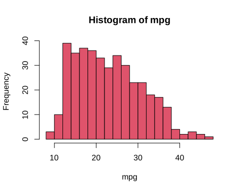
R: hist(mpg, breaks = 15)
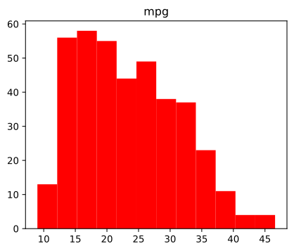
Python: Auto.hist("mpg", bins=12)
A scatterplot matrix shows every pair of a set of variables: pairs() in R, pd.plotting.scatter_matrix() in pandas (which puts histograms on the diagonal). Mileage falls with displacement, horsepower and weight, all strongly and non-linearly.
open_png("lab-r-pairs", 7, 7)
pairs(~ mpg + displacement + horsepower + weight + acceleration, data = Auto, cex = 0.4)
invisible(dev.off())
report("correlations of mpg with displacement, horsepower, weight, acceleration",
       cor(Auto[, c("displacement", "horsepower", "weight", "acceleration")], Auto$mpg))
correlations of mpg with displacement, horsepower, weight, acceleration: -0.8051 -0.7784 -0.8322 0.4233axes = pd.plotting.scatter_matrix(Auto[["mpg", "displacement", "weight"]], figsize=(7, 7), s=8)
save(axes[0, 0].figure, "lab-py-pairs", "png")
report("correlations of mpg with displacement, horsepower, weight, acceleration",
Auto[["displacement", "horsepower", "weight", "acceleration"]].corrwith(Auto["mpg"]))correlations of mpg with displacement, horsepower, weight, acceleration: -0.8051 -0.7784 -0.8322 0.4233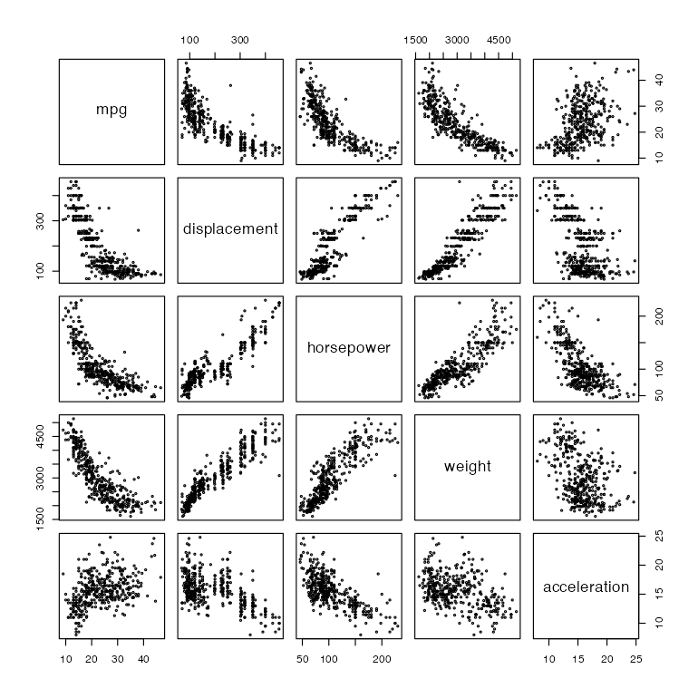
R: pairs(~ mpg + displacement + horsepower + weight + acceleration)
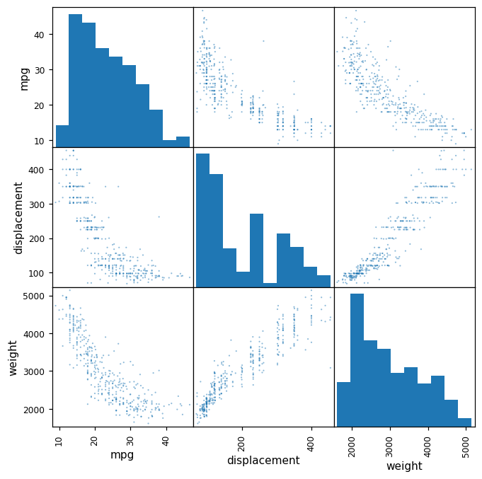
Python: pd.plotting.scatter_matrix(Auto[["mpg", "displacement", "weight"]])
Finally, numerical summaries: R's summary() gives the minimum, quartiles, mean and maximum of each quantitative column and the counts of each qualitative one; pandas' describe() gives the count, mean, standard deviation, minimum, quartiles and maximum.
summary(Auto)
summary(Auto$mpg)
report("mpg: min, 1st quartile, median, mean, 3rd quartile, max", summary(Auto$mpg))
report("weight: mean, standard deviation", c(mean(Auto$weight), sd(Auto$weight)))
mpg cylinders displacement horsepower weight
Min. : 9.00 3: 4 Min. : 68.0 Min. : 46.0 Min. :1613
1st Qu.:17.00 4:199 1st Qu.:105.0 1st Qu.: 75.0 1st Qu.:2225
Median :22.75 5: 3 Median :151.0 Median : 93.5 Median :2804
Mean :23.45 6: 83 Mean :194.4 Mean :104.5 Mean :2978
3rd Qu.:29.00 8:103 3rd Qu.:275.8 3rd Qu.:126.0 3rd Qu.:3615
Max. :46.60 Max. :455.0 Max. :230.0 Max. :5140
acceleration year origin name
Min. : 8.00 Min. :70.00 Min. :1.000 amc matador : 5
1st Qu.:13.78 1st Qu.:73.00 1st Qu.:1.000 ford pinto : 5
Median :15.50 Median :76.00 Median :1.000 toyota corolla : 5
Mean :15.54 Mean :75.98 Mean :1.577 amc gremlin : 4
3rd Qu.:17.02 3rd Qu.:79.00 3rd Qu.:2.000 amc hornet : 4
Max. :24.80 Max. :82.00 Max. :3.000 chevrolet chevette: 4
(Other) :365
Min. 1st Qu. Median Mean 3rd Qu. Max.
9.00 17.00 22.75 23.45 29.00 46.60
... (2 more lines)print(Auto[["mpg", "weight"]].describe())
print(Auto["cylinders"].describe())
print(Auto["mpg"].describe())
s = Auto["mpg"].describe()
report("mpg: min, 1st quartile, median, mean, 3rd quartile, max",
[s["min"], s["25%"], s["50%"], s["mean"], s["75%"], s["max"]])
report("weight: mean, standard deviation", [Auto["weight"].mean(), Auto["weight"].std()]) mpg weight
count 392.000000 392.000000
mean 23.445918 2977.584184
std 7.805007 849.402560
min 9.000000 1613.000000
25% 17.000000 2225.250000
50% 22.750000 2803.500000
75% 29.000000 3614.750000
max 46.600000 5140.000000
count 392
unique 5
top 4
freq 199
Name: cylinders, dtype: int64
count 392.000000
mean 23.445918
std 7.805007
min 9.000000
... (7 more lines)Both compute quartiles the same way (linear interpolation between order statistics, R's default "type 7"), so the summaries agree exactly: for mpg, minimum 9, quartiles 17, 22.75 and 29, mean 23.45, maximum 46.6, as printed in the R edition. In all, every result of the lab that does not involve random numbers is the same in R and Python (confirmed numerically).
Notes on the book
Points where the book's text or code disagrees with an exact computation, or needs a qualification, with the evidence. None changes the chapter's message.
1. Python edition, Exercise 8(f): the bins of pd.cut Python edition p. 66
The exercise creates Elite with pd.cut(college['Top10perc'], [0,0.5,1], labels=['No', 'Yes']). But Top10perc is a percentage, from 1 to 96, not a proportion. With these bins, 774 of the 777 colleges fall outside \((0,1]\) and get a missing value, and the three colleges with Top10perc equal to 1 are labelled "Yes", the opposite of elite. The intended rule ("more than 50% of new students from the top 10% of their class", as in the R edition's college$Top10perc > 50) needs the bins [0, 50, 100], which gives 78 elite colleges in both languages (Exercise 8).
2. The Bayes error rate is quoted as 0.133 and as 0.1304 pp. 39 and 41
Not an error, but easy to misread: 0.133 is the population Bayes error rate (2.11), 0.1304 the error of the Bayes classifier on the 5,000-point test set, an estimate with standard error about 0.005. See Filling the gap 2.8.
3. "A fundamental property ... regardless of the statistical method being used" p. 32
The book says that a monotone decrease of the training MSE and a U-shaped test MSE hold regardless of the data set and the method. Both parts need qualifying. The training error is monotone in flexibility for nested least-squares fits and for smoothing splines (Result 2.3), but not in general: for K-nearest neighbours on the simulated data of Figure 2.17 the training error is 0.055 with \(K=4\) and rises to 0.100 with the more flexible \(K=3\). And the test MSE need not be U-shaped: if \(f\) is exactly linear the smoothing spline's test MSE is smallest at the least flexible end (df 2) and only rises; in Figure 2.10 it is nearly so. Very flexible methods can even show a second descent of the test error (the "double descent" of the book's Chapter 10). As a description of typical behaviour, the statement is right.
4. The College data contain a graduation rate of 118% Exercise 8
Cazenovia College has Grad.Rate 118, impossible for a percentage; it is the only value above 100. It is worth noticing while exploring the data in part (vi)/(h) of the exercise, and is a reminder to check ranges before modelling.
5. Version notes for the Python lab
With current pandas (2.2), read_csv(..., delim_whitespace=True) gives a deprecation warning (use sep=r"\s+"), and Auto.index prints as Index([...], dtype='int64') rather than the Int64Index shown in the book. All the numbers printed in the Python edition's lab are reproduced exactly with numpy 1.26.
2.4 Exercises
All ten exercises of Section 2.4 (R edition pp. 52–57, Python edition pp. 63–67), restated in my own words, with solutions (hidden). The applied exercises are solved in both languages, side by side; the code is the last three blocks of the lab files.
Conceptual
Exercise 2.1. Would a flexible method generally do better or worse than an inflexible one when (a) \(n\) is very large and \(p\) small; (b) \(p\) is very large and \(n\) small; (c) the relationship between predictors and response is highly non-linear; (d) the error variance \(\sigma^2=\Var(\varepsilon)\) is very large? Explain.
Solution
Think in terms of (2.7): flexibility lowers the squared bias and raises the variance, and the variance is larger when there are few observations per parameter and when the noise is large (for a linear smoother it is \(\sigma^2\|\bl(x_0)\|^2\), proportional to \(\sigma^2\)).
- (a) Better. With many observations and few predictors, a flexible fit can be estimated with small variance, so its lower bias wins.
- (b) Worse. With few observations and many predictors, a flexible method has too much freedom: it can fit the training data almost perfectly (overfitting), and its variance is large. A restrictive method is safer.
- (c) Better. An inflexible method has a large bias that more data cannot remove (Example 3, Figure 2.11: the line's squared bias is 12.4).
- (d) Worse. With very noisy data a flexible method chases the noise: its variance grows in proportion to \(\sigma^2\), while the bias it removes does not depend on \(\sigma^2\). The irreducible error is large anyway, so the extra variance is pure loss.
Exercise 2.2. For each scenario, say whether it is regression or classification, whether the interest is inference or prediction, and give \(n\) and \(p\). (a) Data on the top 500 US firms (profit, number of employees, industry, CEO salary), to understand which factors affect CEO salary. (b) Data on 20 earlier product launches (success or failure, price, marketing budget, competitor's price and ten other variables), to tell whether a new product will succeed. (c) Weekly data for 2012 on the % change in the US dollar/euro rate and in the US, British and German stock markets, to predict the exchange-rate change.
Solution
- (a) Regression (salary is quantitative), inference (which factors matter); \(n=500\), \(p=3\) (profit, employees, industry).
- (b) Classification (success/failure), prediction; \(n=20\), \(p=13\) (price, marketing budget, competition price and ten others). With \(p\) close to \(n\), only a very inflexible method is sensible (Exercise 1(b)).
- (c) Regression (a % change), prediction; \(n=52\) weeks, \(p=3\) (the three market changes).
Exercise 2.3. (a) Sketch, on one plot against flexibility, typical curves of the squared bias, the variance, the training error, the test error and the Bayes (irreducible) error. (b) Explain the shape of each.
Solution
(a) Rather than a sketch, here are the five curves computed exactly for Example 1 (the setting of Figure 2.9):
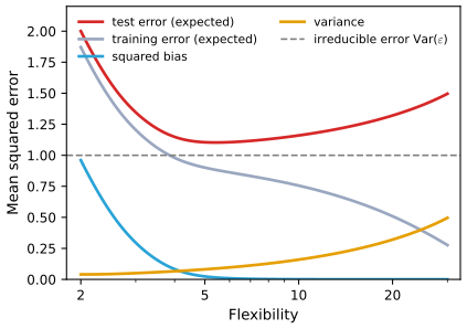
Exercise 2.3. Expected test error (red), expected training error (grey), squared bias (blue), variance (orange) and irreducible error \(\Var(\varepsilon)=1\) (dashed) for Example 1, against the degrees of freedom of a smoothing spline. Code: fig_ex2_3. Download: PDF · SVG(b) Squared bias falls with flexibility: a more flexible family contains functions closer to \(f\) (here it is 0.96 for the line and essentially 0 by df 10). Variance rises: a more flexible fit depends more on individual observations (0.040 at df 2, 0.406 at df 25). Irreducible error is flat: it is a property of the data, not of the method. Test error is the sum of the three (2.7), so it falls while the bias drops faster than the variance grows and rises afterwards: a U, never below the irreducible error. Training error falls monotonically (Result 2.3(a)) and, unlike the test error, goes below the irreducible error, towards 0 as the fit approaches interpolation; the gap between test and training error grows with flexibility (Result 2.3(b)).
Exercise 2.4. Describe three real applications each of (a) classification and (b) regression, with response, predictors and whether the goal is inference or prediction; and (c) three applications of cluster analysis.
Solution
Many answers are possible; for example:
- (a) Spam filtering: response spam/not spam, predictors word and character frequencies; prediction. Credit default: response default yes/no, predictors income, balance, student status; prediction for lending, inference for regulators asking which factors drive default. Clinical diagnosis: response disease present/absent, predictors symptoms and test results; prediction, with inference about which tests are informative.
- (b) House prices: response sale price, predictors size, location, age; prediction (valuation) or inference (the value of a feature). Crop yield: response yield, predictors fertiliser, rainfall, soil; inference about the fertiliser effect. Electricity demand: response tomorrow's load, predictors temperature, day of week, past load; prediction.
- (c) Market segmentation of customers by purchase behaviour; grouping tumour samples by gene expression to find subtypes; grouping documents by topic from word counts.
Exercise 2.5. What are the advantages and disadvantages of a very flexible approach, compared with a less flexible one, for regression or classification? When is each preferable?
Solution
A flexible approach can fit a wide range of shapes, so it has small bias and can capture non-linear effects and interactions. Its disadvantages: high variance and the risk of overfitting, more parameters to estimate (so more data needed), more computation, and a result that is hard to interpret. Prefer it when prediction is the goal, \(n\) is large relative to \(p\), the noise is moderate and the relationship is believed to be complex. Prefer a less flexible approach when interpretation or inference is the goal, \(n\) is small relative to \(p\), the noise is large, or the relationship is believed to be close to the simple form (Figure 2.10).
Exercise 2.6. How do parametric and non-parametric approaches differ? What are the advantages and disadvantages of a parametric approach?
Solution
A parametric approach assumes a functional form for \(f\) with a fixed, finite number of parameters (such as (2.4)) and estimates those parameters; a non-parametric approach makes no such assumption and lets the shape of \(\hat f\) be determined by the data, subject only to smoothness. Advantages of the parametric approach: the problem reduces to estimating a few numbers, so it needs far fewer observations, has lower variance, is cheap to compute and easy to interpret and test. Disadvantages: if the assumed form is far from the true \(f\) the estimate is biased and no amount of data will remove the bias; making the form more flexible to avoid this brings back the variance and the risk of overfitting.
Exercise 2.7. Six training observations with three predictors and a colour: \((0,3,0)\) Red, \((2,0,0)\) Red, \((0,1,3)\) Red, \((0,1,2)\) Green, \((-1,0,1)\) Green, \((1,1,1)\) Red. Predict \(Y\) at \(X_1=X_2=X_3=0\) by K-nearest neighbours: (a) compute the Euclidean distance of each observation from the test point; (b) predict with \(K=1\); (c) with \(K=3\); (d) if the Bayes decision boundary is highly non-linear, would the best \(K\) be large or small?
Solution
(a) The distances are the lengths of the six vectors: \(3\), \(2\), \(\sqrt{10}\approx3.162\), \(\sqrt5\approx2.236\), \(\sqrt2\approx1.414\), \(\sqrt3\approx1.732\).
(b) The nearest is observation 5 (distance 1.414), which is Green: predict Green.
(c) The three nearest are observations 5 (Green, 1.414), 6 (Red, 1.732) and 2 (Red, 2): estimated \(\Pr(\text{Red})=2/3\), predict Red.
(d) Small. A small \(K\) gives a flexible boundary that can follow sharp bends; a large \(K\) averages over wide neighbourhoods and produces a boundary close to linear (Figure 2.16). (Confirmed numerically.)
Applied
Exercise 2.8. The
Collegedata: 18 variables for 777 US colleges (private or public, applications, acceptances, enrolment, the percentage of new students from the top 10% and 25% of their high-school class, undergraduates, tuition, costs, faculty with PhDs, student/faculty ratio, alumni donations, expenditure per student, graduation rate). (a)–(b) Read the file and use the first column (college names) as row names rather than data. (c) Summarise the variables; draw a scatterplot matrix (of the first ten columns in the R edition, ofTop10perc,Apps,Enrollin the Python edition); draw boxplots ofOutstatebyPrivate; createElite(more than 50% of new students from the top 10% of their class), count the elite colleges and draw boxplots ofOutstatebyElite; draw histograms with different numbers of bins; explore further.Solution (R and Python)
Rcollege <- read.csv(file.path(DATA, "College.csv"), stringsAsFactors = TRUE) rownames(college) <- college[, 1] college <- college[, -1] summary(college[, 1:5]) open_png("lab-r-college-pairs", 8, 8) pairs(college[, 1:10], cex = 0.3) invisible(dev.off()) Elite <- rep("No", nrow(college)) Elite[college$Top10perc > 50] <- "Yes" college <- data.frame(college, Elite = as.factor(Elite)) summary(college$Elite) report("median out-of-state tuition: public, private", tapply(college$Outstate, college$Private, median)) report("median out-of-state tuition: not elite, elite", tapply(college$Outstate, college$Elite, median)) open_svg("lab-r-college", 8, 3.6) par(mfrow = c(1, 2)) plot(college$Private, college$Outstate, xlab = "Private", ylab = "Outstate") plot(college$Elite, college$Outstate, xlab = "Elite", ylab = "Outstate") invisible(dev.off()) open_svg("lab-r-college-hist", 8, 6) par(mfrow = c(2, 2)) hist(college$Apps, breaks = 50, main = "Apps (50 bins)", xlab = "") hist(college$Outstate, breaks = 20, main = "Outstate (20 bins)", xlab = "") hist(college$Grad.Rate, breaks = 10, main = "Grad.Rate (10 bins)", xlab = "") hist(college$S.F.Ratio, breaks = 25, main = "S.F.Ratio (25 bins)", xlab = "") invisible(dev.off()) college$AcceptRate <- college$Accept / college$Apps report("acceptance rate: median for public, private", tapply(college$AcceptRate, college$Private, median)) report("correlation of Expend and Grad.Rate", cor(college$Expend, college$Grad.Rate)) college[college$Grad.Rate > 100, c("Private", "Grad.Rate")] # a graduation rate above 100%Private Apps Accept Enroll Top10perc No :212 Min. : 81 Min. : 72 Min. : 35 Min. : 1.00 Yes:565 1st Qu.: 776 1st Qu.: 604 1st Qu.: 242 1st Qu.:15.00 Median : 1558 Median : 1110 Median : 434 Median :23.00 Mean : 3002 Mean : 2019 Mean : 780 Mean :27.56 3rd Qu.: 3624 3rd Qu.: 2424 3rd Qu.: 902 3rd Qu.:35.00 Max. :48094 Max. :26330 Max. :6392 Max. :96.00 No Yes 699 78 median out-of-state tuition: public, private: 6609 11200 median out-of-state tuition: not elite, elite: 9556 16950 acceptance rate: median for public, private: 0.7443 0.7886 correlation of Expend and Grad.Rate: 0.3903 Private Grad.Rate Cazenovia College Yes 118Pythoncollege = pd.read_csv(os.path.join(DATA, "College.csv")) college3 = college.rename({"Unnamed: 0": "College"}, axis=1) college = college3.set_index("College") print(college.iloc[:, :5].describe(include="all")) axes = pd.plotting.scatter_matrix(college[["Top10perc", "Apps", "Enroll"]], figsize=(7, 7), s=6) save(axes[0, 0].figure, "lab-py-college-pairs", "png") college["Elite"] = pd.cut(college["Top10perc"], [0, 50, 100], labels=["No", "Yes"]) # (50, 100] means > 50% print(college["Elite"].value_counts()) report("median out-of-state tuition: public, private", college.groupby("Private")["Outstate"].median()) report("median out-of-state tuition: not elite, elite", college.groupby("Elite", observed=True)["Outstate"].median()) fig, axes = subplots(1, 2, figsize=(8, 3.6)) college.boxplot("Outstate", by="Private", ax=axes[0], grid=False) college.boxplot("Outstate", by="Elite", ax=axes[1], grid=False) fig.suptitle("") save(fig, "lab-py-college") fig, axes = subplots(2, 2, figsize=(8, 6)) for ax, (col, bins) in zip(axes.ravel(), [("Apps", 50), ("Outstate", 20), ("Grad.Rate", 10), ("S.F.Ratio", 25)]): college[col].plot.hist(ax=ax, bins=bins) ax.set_title("%s (%d bins)" % (col, bins)) save(fig, "lab-py-college-hist") college["AcceptRate"] = college["Accept"] / college["Apps"] report("acceptance rate: median for public, private", college.groupby("Private")["AcceptRate"].median()) report("correlation of Expend and Grad.Rate", college["Expend"].corr(college["Grad.Rate"])) print(college.loc[college["Grad.Rate"] > 100, ["Private", "Grad.Rate"]]) # a graduation rate above 100%Private Apps Accept Enroll Top10perc count 777 777.000000 777.000000 777.000000 777.000000 unique 2 NaN NaN NaN NaN top Yes NaN NaN NaN NaN freq 565 NaN NaN NaN NaN mean NaN 3001.638353 2018.804376 779.972973 27.558559 std NaN 3870.201484 2451.113971 929.176190 17.640364 min NaN 81.000000 72.000000 35.000000 1.000000 25% NaN 776.000000 604.000000 242.000000 15.000000 50% NaN 1558.000000 1110.000000 434.000000 23.000000 75% NaN 3624.000000 2424.000000 902.000000 35.000000 max NaN 48094.000000 26330.000000 6392.000000 96.000000 Elite No 699 Yes 78 Name: count, dtype: int64 median out-of-state tuition: public, private: 6609 11200 median out-of-state tuition: not elite, elite: 9556 16950 acceptance rate: median for public, private: 0.7443 0.7886 correlation of Expend and Grad.Rate: 0.3903 Private Grad.Rate College Cazenovia College Yes 118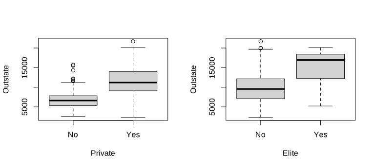
R
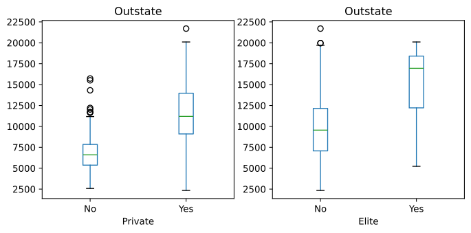
Python
Results. There are 565 private and 212 public colleges, and 78 elite colleges (699 not elite). Private colleges charge more out-of-state tuition (median $11,200 against $6,609), and elite colleges much more (median $16,950 against $9,556). Private colleges accept a slightly higher share of applicants (median 0.789 against 0.744). Expenditure per student and graduation rate are positively correlated (0.39). One record is impossible: Cazenovia College's graduation rate of 118% (see Notes on the book). The histograms (R, Python) show strongly right-skewed
Apps, roughly symmetricOutstateandGrad.Rate. The Python edition's own code forElitemislabels the colleges (Notes on the book); the bins[0, 50, 100]used here give the same 78 as the R edition's rule.Exercise 2.9. The
Autodata without missing values. (a) Which predictors are quantitative and which qualitative? (b) What is the range of each quantitative predictor? (c) Its mean and standard deviation? (d) Repeat (b)–(c) after removing observations 10 to 85. (e) Explore the predictors graphically. (f) Which variables look useful for predictingmpg?Solution (R and Python)
RAuto <- na.omit(read.csv(file.path(DATA, "Auto.csv"), na.strings = "?", stringsAsFactors = TRUE)) quant <- c("mpg", "cylinders", "displacement", "horsepower", "weight", "acceleration", "year") sapply(Auto[, quant], range) for (v in quant) report(paste(v, "min, max, mean, sd"), c(range(Auto[[v]]), mean(Auto[[v]]), sd(Auto[[v]]))) sub <- Auto[-(10:85), ] report("rows left after removing observations 10 to 85", nrow(sub)) for (v in quant) report(paste("subset", v, "min, max, mean, sd"), c(range(sub[[v]]), mean(sub[[v]]), sd(sub[[v]]))) report("correlation of mpg with cylinders, displacement, horsepower, weight, acceleration, year", cor(Auto[, quant])[1, -1]) report("mean mpg by origin (1 America, 2 Europe, 3 Japan)", tapply(Auto$mpg, Auto$origin, mean))mpg cylinders displacement horsepower weight acceleration year [1,] 9.0 3 68 46 1613 8.0 70 [2,] 46.6 8 455 230 5140 24.8 82 mpg min, max, mean, sd: 9.0000 46.6000 23.4459 7.8050 cylinders min, max, mean, sd: 3.0000 8.0000 5.4719 1.7058 displacement min, max, mean, sd: 68.0000 455.0000 194.4120 104.6440 horsepower min, max, mean, sd: 46.0000 230.0000 104.4694 38.4912 weight min, max, mean, sd: 1613.0000 5140.0000 2977.5842 849.4026 acceleration min, max, mean, sd: 8.0000 24.8000 15.5413 2.7589 year min, max, mean, sd: 70.0000 82.0000 75.9796 3.6837 rows left after removing observations 10 to 85: 316 subset mpg min, max, mean, sd: 11.0000 46.6000 24.4044 7.8673 subset cylinders min, max, mean, sd: 3.0000 8.0000 5.3734 1.6542 subset displacement min, max, mean, sd: 68.0000 455.0000 187.2405 99.6784 subset horsepower min, max, mean, sd: 46.0000 230.0000 100.7215 35.7089 subset weight min, max, mean, sd: 1649.0000 4997.0000 2935.9715 811.3002 subset acceleration min, max, mean, sd: 8.5000 24.8000 15.7269 2.6937 subset year min, max, mean, sd: 70.0000 82.0000 77.1456 3.1062 correlation of mpg with cylinders, displacement, horsepower, weight, acceleration, year: -0.7776 -0.8051 -0.7784 -0.8322 0.4233 0.5805 mean mpg by origin (1 America, 2 Europe, 3 Japan): 20.0335 27.6029 30.4506PythonAuto = pd.read_csv(os.path.join(DATA, "Auto.csv"), na_values=["?"]).dropna() quant = ["mpg", "cylinders", "displacement", "horsepower", "weight", "acceleration", "year"] print(Auto[quant].agg(["min", "max"])) for v in quant: report(v + " min, max, mean, sd", [Auto[v].min(), Auto[v].max(), Auto[v].mean(), Auto[v].std()]) sub = Auto.drop(Auto.index[9:85]) # observations 10 to 85 (positions 9 to 84) report("rows left after removing observations 10 to 85", len(sub)) for v in quant: report("subset " + v + " min, max, mean, sd", [sub[v].min(), sub[v].max(), sub[v].mean(), sub[v].std()]) report("correlation of mpg with cylinders, displacement, horsepower, weight, acceleration, year", Auto[quant].corr().loc["mpg"].iloc[1:]) report("mean mpg by origin (1 America, 2 Europe, 3 Japan)", Auto.groupby("origin")["mpg"].mean())mpg cylinders displacement horsepower weight acceleration year min 9.0 3 68.0 46.0 1613 8.0 70 max 46.6 8 455.0 230.0 5140 24.8 82 mpg min, max, mean, sd: 9.0000 46.6000 23.4459 7.8050 cylinders min, max, mean, sd: 3.0000 8.0000 5.4719 1.7058 displacement min, max, mean, sd: 68.0000 455.0000 194.4120 104.6440 horsepower min, max, mean, sd: 46.0000 230.0000 104.4694 38.4912 weight min, max, mean, sd: 1613.0000 5140.0000 2977.5842 849.4026 acceleration min, max, mean, sd: 8.0000 24.8000 15.5413 2.7589 year min, max, mean, sd: 70.0000 82.0000 75.9796 3.6837 rows left after removing observations 10 to 85: 316 subset mpg min, max, mean, sd: 11.0000 46.6000 24.4044 7.8673 subset cylinders min, max, mean, sd: 3.0000 8.0000 5.3734 1.6542 subset displacement min, max, mean, sd: 68.0000 455.0000 187.2405 99.6784 subset horsepower min, max, mean, sd: 46.0000 230.0000 100.7215 35.7089 subset weight min, max, mean, sd: 1649.0000 4997.0000 2935.9715 811.3002 subset acceleration min, max, mean, sd: 8.5000 24.8000 15.7269 2.6937 subset year min, max, mean, sd: 70.0000 82.0000 77.1456 3.1062 correlation of mpg with cylinders, displacement, horsepower, weight, acceleration, year: -0.7776 -0.8051 -0.7784 -0.8322 0.4233 0.5805 mean mpg by origin (1 America, 2 Europe, 3 Japan): 20.0335 27.6029 30.4506(a) Quantitative:
mpg,cylinders,displacement,horsepower,weight,acceleration,year. Qualitative:name, andorigin, which is a code (1 America, 2 Europe, 3 Japan) even though it is stored as a number. (cylinderstakes only five values and can reasonably be treated as qualitative too, as in the lab.)Variable min max mean sd mean, rows 10–85 removed sd, rows 10–85 removed mpg 9 46.6 23.45 7.81 24.40 7.87 cylinders 3 8 5.47 1.71 5.37 1.65 displacement 68 455 194.41 104.64 187.24 99.68 horsepower 46 230 104.47 38.49 100.72 35.71 weight 1613 5140 2977.58 849.40 2935.97 811.30 acceleration 8 24.8 15.54 2.76 15.73 2.69 year 70 82 75.98 3.68 77.15 3.11 (d) 316 cars remain. The ranges barely change (the minimum
mpgbecomes 11, the weight range 1649–4997, acceleration from 8.5), but the means shift: the removed rows are mostly early-1970s cars, so the remaining cars are newer (mean year 77.1), lighter and more economical.(e)–(f) The scatterplot matrix of the lab shows that
mpgfalls withdisplacement,horsepowerandweight(correlations \(-0.81\), \(-0.78\), \(-0.83\)), curving rather than straight, and withcylinders(\(-0.78\)); it rises withyear(0.58) and modestly withacceleration(0.42); and Japanese and European cars average more miles per gallon (30.5 and 27.6) than American ones (20.0). Displacement, horsepower, weight and cylinders are strongly correlated with each other, so they carry largely the same information. All of these look useful for predictingmpg; weight (or horsepower) and year are a natural start, perhaps with a non-linear term (Chapters 3 and 7).Exercise 2.10. The
Bostonhousing data (506 census tracts of the Boston area, 13 variables). (a) How many rows and columns, and what do they represent? (b) Make pairwise scatterplots and describe them. (c) Are any predictors associated with the per-capita crime ratecrim? (d) Are there tracts with particularly high crime rates, tax rates or pupil-teacher ratios? (e) How many tracts bound the Charles river? (f) What is the median pupil-teacher ratio? (g) Which tract has the lowest median home valuemedv, and how do its other values compare with the ranges? (h) How many tracts average more than seven rooms per dwelling, and more than eight? Comment on the latter.Solution (R and Python)
Rlibrary(ISLR2) dim(Boston) report("correlation of crim with the other variables", cor(Boston)[1, -1]) sapply(Boston[, c("crim", "tax", "ptratio")], range) report("tracts with crim > 20, tax > 600, ptratio > 20", c(sum(Boston$crim > 20), sum(Boston$tax > 600), sum(Boston$ptratio > 20))) report("tracts bounding the Charles river", sum(Boston$chas)) report("median pupil-teacher ratio", median(Boston$ptratio)) i <- which.min(Boston$medv) report("tract with the lowest median value (row), and how many share it", c(i, sum(Boston$medv == min(Boston$medv)))) Boston[Boston$medv == min(Boston$medv), ] report("percentile of that tract for crim, lstat, ptratio", sapply(c("crim", "lstat", "ptratio"), function(v) mean(Boston[[v]] <= Boston[i, v]))) report("tracts averaging more than 7 and more than 8 rooms", c(sum(Boston$rm > 7), sum(Boston$rm > 8))) report("tracts with more than 8 rooms: mean crim, lstat, medv", colMeans(Boston[Boston$rm > 8, c("crim", "lstat", "medv")]))[1] 506 13 correlation of crim with the other variables: -0.2005 0.4066 -0.0559 0.4210 -0.2192 0.3527 -0.3797 0.6255 0.5828 0.2899 0.4556 -0.3883 crim tax ptratio [1,] 0.00632 187 12.6 [2,] 88.97620 711 22.0 tracts with crim > 20, tax > 600, ptratio > 20: 18 137 201 tracts bounding the Charles river: 35 median pupil-teacher ratio: 19.0500 tract with the lowest median value (row), and how many share it: 399 2 crim zn indus chas nox rm age dis rad tax ptratio lstat medv 399 38.3518 0 18.1 0 0.693 5.453 100 1.4896 24 666 20.2 30.59 5 406 67.9208 0 18.1 0 0.693 5.683 100 1.4254 24 666 20.2 22.98 5 percentile of that tract for crim, lstat, ptratio: 0.9881 0.9783 0.8893 tracts averaging more than 7 and more than 8 rooms: 64 13 tracts with more than 8 rooms: mean crim, lstat, medv: 0.7188 4.3100 44.2000PythonBoston = pd.read_csv(os.path.join(DATA, "Boston.csv"), index_col=0) print(Boston.shape) report("correlation of crim with the other variables", Boston.corr().loc["crim"].iloc[1:]) print(Boston[["crim", "tax", "ptratio"]].agg(["min", "max"])) report("tracts with crim > 20, tax > 600, ptratio > 20", [(Boston["crim"] > 20).sum(), (Boston["tax"] > 600).sum(), (Boston["ptratio"] > 20).sum()]) report("tracts bounding the Charles river", Boston["chas"].sum()) report("median pupil-teacher ratio", Boston["ptratio"].median()) i = int(np.argmin(Boston["medv"])) report("tract with the lowest median value (row), and how many share it", [i + 1, (Boston["medv"] == Boston["medv"].min()).sum()]) print(Boston[Boston["medv"] == Boston["medv"].min()]) report("percentile of that tract for crim, lstat, ptratio", [(Boston[v] <= Boston[v].iloc[i]).mean() for v in ["crim", "lstat", "ptratio"]]) report("tracts averaging more than 7 and more than 8 rooms", [(Boston["rm"] > 7).sum(), (Boston["rm"] > 8).sum()]) report("tracts with more than 8 rooms: mean crim, lstat, medv", Boston.loc[Boston["rm"] > 8, ["crim", "lstat", "medv"]].mean())(506, 13) correlation of crim with the other variables: -0.2005 0.4066 -0.0559 0.4210 -0.2192 0.3527 -0.3797 0.6255 0.5828 0.2899 0.4556 -0.3883 crim tax ptratio min 0.00632 187 12.6 max 88.97620 711 22.0 tracts with crim > 20, tax > 600, ptratio > 20: 18 137 201 tracts bounding the Charles river: 35 median pupil-teacher ratio: 19.0500 tract with the lowest median value (row), and how many share it: 399 2 crim zn indus chas nox ... rad tax ptratio lstat medv 399 38.3518 0.0 18.1 0 0.693 ... 24 666 20.2 30.59 5.0 406 67.9208 0.0 18.1 0 0.693 ... 24 666 20.2 22.98 5.0 [2 rows x 13 columns] percentile of that tract for crim, lstat, ptratio: 0.9881 0.9783 0.8893 tracts averaging more than 7 and more than 8 rooms: 64 13 tracts with more than 8 rooms: mean crim, lstat, medv: 0.7188 4.3100 44.2000(a) 506 rows, one per census tract; 13 columns: crime rate, proportion of large residential lots, proportion of industry, the Charles river indicator, nitrogen oxides, rooms per dwelling, proportion of old houses, distance to employment centres, highway access, tax rate, pupil-teacher ratio, percentage of lower-status population, and median home value (R:
library(ISLR2); Python:Boston.csv).(b)–(c) Crime is highest where highway access (
rad, correlation 0.63) and the tax rate (0.58) are high, and also rises withlstat(0.46),nox(0.42) andindus(0.41); it falls with home value (\(-0.39\)) and distance to employment centres (\(-0.38\)). The relationships are far from linear: most tracts have crime rates near zero and a few have very large ones.(d) The crime rate ranges from 0.006 to 89.0 per capita, extremely skewed: 18 tracts exceed 20. The tax rate ranges from 187 to 711, with 137 tracts above 600 (a block of tracts sharing the value 666). The pupil-teacher ratio ranges from 12.6 to 22.0, without isolated extremes (201 tracts above 20).
(e) 35 tracts bound the Charles river. (f) The median pupil-teacher ratio is 19.05.
(g) Two tracts share the lowest median value, 5 (thousand dollars): rows 399 and 406. Row 399 has a crime rate of 38.4 (above 98.8% of tracts),
lstat30.6 (above 97.8%), all houses built before 1940 (age100), high industry (18.1), high nitrogen oxides, maximal highway access (24), tax rate 666 and pupil-teacher ratio 20.2: close to the worst end of almost every range.(h) 64 tracts average more than seven rooms, 13 more than eight. The latter are prosperous: mean crime rate 0.72, mean
lstat4.3% and mean median value 44.2 (the maximum, 50, is a censoring value in these data).
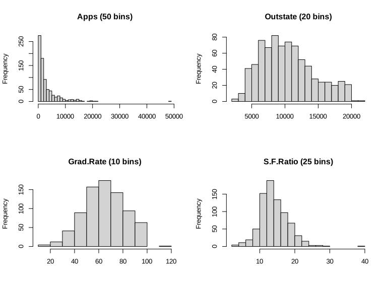
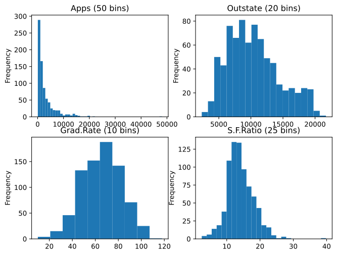
Demonstrations for this chapter
Each demonstration runs in the browser on the data used for this page's figures (exported by the Python code) and links back to these notes. The ▶ Demo boxes above open them already set to the case under discussion.
| Demonstration | What you can see | Sections and results |
|---|---|---|
| Training and test error as flexibility grows | Smoothing-spline fits of any degrees of freedom to the three simulated examples, the expected training and test MSE curves, the errors of the current fit, and new training samples. Presets: 1 the line; 2 near the best df; 3 overfitted; 4 Example 2; 5 Example 3. | 2.2.1; Definition 2.2, Result 2.3; Figures 2.9–2.11 |
| The bias-variance decomposition | Fits from many training sets, their average and the true \(f\); the exact squared bias, variance and test MSE at a chosen \(x_0\) and on average, against a running simulation estimate; the curves of Figure 2.12. Presets: 1 stiff; 2 balanced; 3 wiggly; 4 Example 3 line; 5 Example 2. | 2.2.2; Result 2.4, Filling the gap 2.5; Figure 2.12 |
| The Bayes classifier and K-nearest neighbours | The Bayes regions and boundary, KNN regions for any \(K\), the neighbourhood of a clicked point with the estimate (2.12), and the training and test error against \(1/K\). Presets: 1 Bayes; 2 three neighbours; 3 K = 10; 4 K = 1; 5 K = 100. | 2.2.3; Results 2.5, 2.6, Definition 2.3; Figures 2.13–2.17 |
Related demonstrations in the companion courses: least squares versus k-nearest neighbours (Statistical Learning: Theory and Methods) and bias and variance (Bayesian and Probabilistic Machine Learning). The code for this page: code/ch02_statistical_learning.py (figures and demonstration data), code/ch02_lab.R and code/ch02_lab.py (the lab and the applied exercises); see the code index.
References
- James, G., Witten, D., Hastie, T. and Tibshirani, R. (2021). An Introduction to Statistical Learning with Applications in R, 2nd edition. Springer, New York. Chapter 2, pp. 15–57. www.statlearning.com.
- James, G., Witten, D., Hastie, T., Tibshirani, R. and Taylor, J. (2023). An Introduction to Statistical Learning with Applications in Python. Springer, Cham. Chapter 2, pp. 15–67.
- Cover, T. and Hart, P. (1967). Nearest neighbor pattern classification. IEEE Transactions on Information Theory, 13(1), 21–27.
- Craven, P. and Wahba, G. (1979). Smoothing noisy data with spline functions. Numerische Mathematik, 31(4), 377–403.
- Duchon, J. (1977). Splines minimizing rotation-invariant semi-norms in Sobolev spaces. In Constructive Theory of Functions of Several Variables, Lecture Notes in Mathematics 571, Springer, 85–100.
- Fix, E. and Hodges, J. L. (1951). Discriminatory analysis: nonparametric discrimination, consistency properties. Technical Report 4, USAF School of Aviation Medicine, Randolph Field, Texas.
- Green, P. J. and Silverman, B. W. (1994). Nonparametric Regression and Generalized Linear Models: A Roughness Penalty Approach. Chapman and Hall, London.
- Harrison, D. and Rubinfeld, D. L. (1978). Hedonic housing prices and the demand for clean air. Journal of Environmental Economics and Management, 5(1), 81–102.
- Hastie, T., Tibshirani, R. and Friedman, J. (2009). The Elements of Statistical Learning: Data Mining, Inference, and Prediction, 2nd edition. Springer, New York.
- Reinsch, C. H. (1967). Smoothing by spline functions. Numerische Mathematik, 10(3), 177–183.
- Wahba, G. (1990). Spline Models for Observational Data. SIAM, Philadelphia.
- Wolpert, D. H. (1996). The lack of a priori distinctions between learning algorithms. Neural Computation, 8(7), 1341–1390.
The numerical statements in the text (the smoothing-spline computations against two independent implementations, the exact bias, variance and error curves against simulation, the Bayes error rate, the K-nearest-neighbour error rates against an independent implementation, the agreement of the R and Python labs with each other and with the output printed in the two editions, and the exercise results) were confirmed numerically.