Chapter 7. Multivariate Analysis
When many variables are measured on the same subjects, their joint structure carries information that no single variable shows. This chapter reduces such a data matrix to a few new variables, the principal components, chosen to keep as much of the variability as possible. Behind the method sit three linear-algebra facts: orthogonal projection, the singular value decomposition, and the theorem that truncating the SVD gives the best low-rank approximation of a matrix. These notes follow Holmes and Huber (2019), Modern Statistics for Modern Biology, Chapter 7, and prove the results that the book uses without derivation.
Ch. 1 Discrete data Ch. 2 Statistical modeling Ch. 3 Data visualization Ch. 4 Mixture models Ch. 5 Clustering Ch. 6 Testing Ch. 7 Multivariate analysis Ch. 8 Count data and GLMs Ch. 9 Heterogeneous data Ch. 10 Networks and trees Ch. 11 Image data Ch. 12 Supervised learning Ch. 13 Experimental design
How to read these notes
They follow the book. Sections carry the book's numbers (7.2, 7.6.3, ...) and its titles; displayed equations that appear in the book carry its equation numbers, e.g. (7.5). Equations without a number are steps the book does not show. The book's Questions are answered where they arise.
Filling the gaps. The book is deliberately light on algebra. Wherever it states a result without proof (the SVD exists, truncating it is optimal, the principal components are eigenvectors, the arrows of a correlation circle are correlations, ...), an orange Filling the gap box gives a complete argument. Proofs start hidden: open one with its bar, or use the button below.
Figures and demonstrations. Every figure computed from data is redrawn from scratch by the course R code, and every number quoted in these notes is checked numerically. The ▶ Demo boxes open an interactive demonstration already set to the case under discussion.
Main reference
S. Holmes and W. Huber, Modern Statistics for Modern Biology, Cambridge University Press (2019), Chapter 7. Section, equation, figure, question and exercise numbers below refer to this book. The text and code here are my own; results are cited by their place in the book.
The chapter at a glance
- 7.2 Data come as an \(n\times p\) matrix (rows: subjects, columns: variables). Centring is multiplication by the projection \(\Hc=\I-\one\one^\T/n\); the covariance matrix is \(\X^\T\Hc\X/(n-1)\), the correlation matrix is that of the standardised columns. Correlations do not change with units; covariances do.
- 7.3–7.4 Projecting a cloud of points onto a line: regression minimises vertical (or horizontal) distances, the principal component line minimises perpendicular distances. Pythagoras splits the total variance into the variance along a line and the mean squared distance to it, so the best-fitting line is the line of largest variance.
- 7.5–7.6 Every matrix is a sum of rank-one pieces \(s_k\mathbf{u}_k\mathbf{v}_k^\T\) with orthonormal \(\mathbf{u}\)'s and \(\mathbf{v}\)'s (the SVD, Theorem 7.3). Keeping the first \(k\) pieces is the best rank-\(k\) approximation (Eckart–Young–Mirsky, Theorem 7.4). The right singular vectors of the centred data matrix are the eigenvectors of its covariance, and they are the principal component loadings (Theorem 7.6).
- 7.7–7.8 Reading a PCA: the scree plot of eigenvalues, the principal plane of scores, the correlation circle and the biplot; supplementary individuals and variables; weighted PCA; and why components with nearly equal eigenvalues must not be interpreted one at a time.
Notation. \(\X\in\R^{n\times p}\) is the data matrix with rows \(\mathbf{x}_i^\T\) (observations) and columns \(\mathbf{x}_{\cdot j}\) (variables); \(\one\) is the vector of ones and \(\I\) the identity. The book writes \(t(\cdot)\) or \(^t\) for the transpose; these notes write \(^\T\). \(\|\mathbf{a}\|\) is the Euclidean norm, \(\|\mathbf{A}\|_\F=(\sum_{ij}a_{ij}^2)^{1/2}\) the Frobenius norm and \(\|\mathbf{A}\|_2=\max_{\|\mathbf{w}\|=1}\|\mathbf{A}\mathbf{w}\|\) the spectral norm of a matrix. Sample variances use the divisor \(n-1\) unless said otherwise.
Prerequisites. Matrix multiplication, transpose, inverse, orthogonal matrices, and the spectral theorem for symmetric matrices (every real symmetric matrix is \(\mathbf{Q}\Lam\mathbf{Q}^\T\) with \(\mathbf{Q}\) orthogonal and \(\Lam\) real diagonal). Linear regression by least squares (Chapter 8 of the book treats it in depth).
7.2 What are the data? Matrices and their motivation
The objects of this chapter are rectangular tables of numbers. The book's examples show how varied they are: three shell measurements of 48 painted turtles (Jolicoeur and Mosimann 1960); the results of 33 athletes in the ten events of the 1988 Olympic decathlon; expression of 156 genes in 30 sorted T-cell samples (Holmes et al. 2005); counts of bacterial taxa in environmental samples, mostly zeros; RNA-seq read counts; and mass-spectrometry intensities. Two warnings come with them. First, the orientation is a convention: most of statistics puts subjects in rows, while the RNA-seq tradition puts genes in rows, so a matrix must be transposed before it is fed to a method that expects the other layout. Second, sample information (sex, cell type, genotype) is often hidden in row names; it belongs in its own columns or, better, in a data container such as Bioconductor's SummarizedExperiment.
Definition 7.1 (data matrix) Section 7.2
A data matrix is \(\X=(x_{ij})\in\R^{n\times p}\): row \(i\) holds the \(p\) measurements on observation \(i\), column \(j\) the \(n\) values of variable \(j\). In R, X[5, 3] is \(x_{53}\), the third variable of the fifth observation (Question 7.1).
Question 7.1 and the Task on zeros. The columns are usually called variables or features (genes, taxa, peaks, events); the rows are samples, subjects or specimens; a cell is one measurement of one variable on one subject. Zeros are frequent in count and intensity matrices because "not detected" is recorded as zero; the share of zeros is the proportion of cells equal to 0, computed in R by mean(X == 0).
7.2.1 Low-dimensional data summaries and preparation
A single number such as a mean is a zero-dimensional summary of a variable; a correlation coefficient summarises a two-dimensional scatterplot in one number,
\[ \hat\rho=\frac{\sum_{i=1}^n (x_i-\bar x)(y_i-\bar y)}{\sqrt{\sum_{i=1}^n (x_i-\bar x)^2}\,\sqrt{\sum_{i=1}^n (y_i-\bar y)^2}}. \tag{7.1} \]Applied to a matrix, R's cor returns all \(p(p-1)/2\) pairwise correlations at once. Everything that follows uses these quantities in matrix form, so we set them up carefully.
Filling the gap 7.1: centring, covariance and correlation as matrix operations Section 7.2.1, (7.1)
The book computes means, covariances and correlations with R functions. Writing them as matrix products explains why they behave as they do.
Derivation
Centring is a projection. The vector of column means is \(\bar{\mathbf{x}}=\X^\T\one/n\). Let \(\Hc=\I_n-\one\one^\T/n\) (the centring matrix). Then \(\Hc\X=\X-\one\bar{\mathbf{x}}^\T\) subtracts each column mean. \(\Hc\) is symmetric, \(\Hc\one=\mathbf{0}\), and \(\Hc^2=\I-2\one\one^\T/n+\one(\one^\T\one)\one^\T/n^2=\Hc\) because \(\one^\T\one=n\). A symmetric idempotent matrix is an orthogonal projection: \(\Hc\) projects onto the subspace orthogonal to \(\one\), of dimension \(n-1\). Centred columns therefore always sum to zero, and a centred matrix has rank at most \(\min(n-1,p)\).
Covariance. The sample covariance matrix is
\[ \Sh=\frac{1}{n-1}(\Hc\X)^\T(\Hc\X)=\frac{1}{n-1}\X^\T\Hc\X, \]using \(\Hc^\T\Hc=\Hc^2=\Hc\). Its \((j,l)\) entry is \(\frac{1}{n-1}\sum_i(x_{ij}-\bar x_j)(x_{il}-\bar x_l)\). For any vector of coefficients \(\mathbf{a}\in\R^p\), the new variable \(\X\mathbf{a}\) (one value per observation) has sample variance
\[ \var(\X\mathbf{a})=\frac{\|\Hc\X\mathbf{a}\|^2}{n-1}=\mathbf{a}^\T\Sh\mathbf{a}\ \ge 0. \]So \(\Sh\) is positive semi-definite, and this identity, "the variance of a linear combination is a quadratic form in \(\Sh\)", is the engine of PCA.
Correlation. Let \(\D=\diag(s_1^2,\dots,s_p^2)\) hold the variances \(s_j^2=S_{jj}\) and let \(\Z_{\rm std}=\Hc\X\D^{-1/2}\) be the standardised matrix (what R's scale returns: each column centred and divided by its standard deviation). Then
Entry \((j,l)\) is (7.1) for columns \(j\) and \(l\). Geometrically, (7.1) is the cosine of the angle between the centred vectors \(\Hc\mathbf{x}_{\cdot j}\) and \(\Hc\mathbf{x}_{\cdot l}\) in \(\R^n\): \(\hat\rho=\langle\mathbf{a},\mathbf{b}\rangle/(\|\mathbf{a}\|\|\mathbf{b}\|)\). The Cauchy–Schwarz inequality \(|\langle\mathbf{a},\mathbf{b}\rangle|\le\|\mathbf{a}\|\|\mathbf{b}\|\) gives \(|\hat\rho|\le1\), with equality exactly when one centred vector is a multiple of the other, i.e. when the points lie on a straight line. This is the book's remark that "the correlation coefficient is simply the vector product of the centered and scaled variables" (up to the factor \(1/(n-1)\)). \(\Rm\) is positive semi-definite (it is \(\D^{-1/2}\Sh\D^{-1/2}\)), has unit diagonal, and its trace is \(p\): standardised data always have total variance \(p\). ∎
Question 7.2. For the turtles the correlation matrix is symmetric with unit diagonal and every off-diagonal entry is between 0.96 and 0.98: the three measurements nearly carry the same information. Question 7.3 asks for all pairwise scatterplots (Figure 7.2); they all look like tight lines, so the "true dimension" of these data is close to one, an overall size.
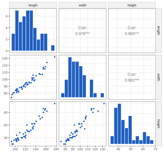
fig_7_2. Reproduces Holmes and Huber (2019), Figure 7.2. Download: PDF · SVGQuestion 7.4. For the decathlon the heat map of correlations (Figure 7.3) groups the events by hierarchical clustering into running (100 m, 110 m hurdles, 400 m, 1500 m), throwing (shot put, discus, javelin) and jumping, with the long jump negatively correlated with the running times: a fast sprinter has small times and long jumps.
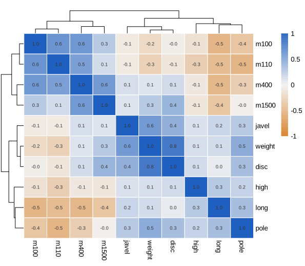
fig_7_3. Reproduces Holmes and Huber (2019), Figure 7.3. Download: PDF · SVG7.2.2 Preprocessing the data
Variables measured in different units have different baselines and spreads: in the decathlon the 110 m hurdle times have standard deviation 0.51 s, the 1500 m times 13.66 s. Centring subtracts each column mean; scaling (standardising) then divides by the standard deviation. R's scale does both. Question 7.5: the turtles' means are 124.7, 95.4 and 46.3 mm and their standard deviations 20.5, 12.7 and 8.4 mm; after scale the means are zero (to rounding, about \(10^{-16}\)) and the standard deviations one. Figure 7.4 shows the standardised width and height coloured by sex.
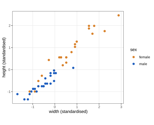
fig_7_4. Reproduces Holmes and Huber (2019), Figure 7.4. Download: PDF · SVGRunning events are recorded as times (smaller is better) while throws and jumps are distances (larger is better), which makes good performances negatively correlated across event types. The book converts times to speeds, distance divided by time, so that larger is better everywhere; Figure 7.5 is the new correlation heat map.
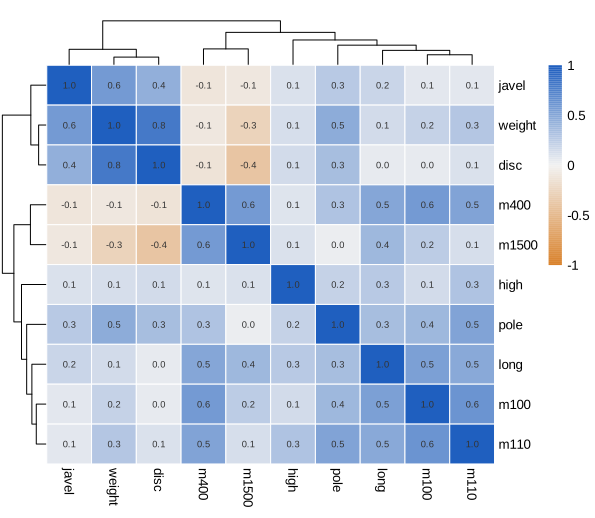
fig_7_5. Reproduces Holmes and Huber (2019), Figure 7.5. Download: PDF · SVGFilling the gap 7.2: what changes of units do to covariances and correlations Section 7.2.2
The book says that scaling makes variables comparable and that times can be turned into speeds. Here is exactly what each operation changes.
Derivation
Affine changes of units. Suppose each variable is recoded as \(x'_{ij}=c_j+b_jx_{ij}\) (centimetres to inches, Celsius to Fahrenheit), i.e. \(\X'=\one\mathbf{c}^\T+\X\B\) with \(\B=\diag(b_1,\dots,b_p)\). Centring removes \(\one\mathbf{c}^\T\) (because \(\Hc\one=\mathbf{0}\)), so \(\Sh'=\B\Sh\B\): covariance entries are multiplied by \(b_jb_l\), variances by \(b_j^2\). The standard deviations become \(|b_j|s_j\), hence
\[ R'_{jl}=\frac{b_jb_lS_{jl}}{|b_j|s_j\,|b_l|s_l}=\operatorname{sign}(b_jb_l)\,R_{jl}. \]Correlations are invariant under positive rescaling and only flip sign when a variable's direction is reversed (\(b_j<0\)). This is why the correlation matrix, and PCA computed from it, does not depend on the units chosen, while the covariance matrix does (Filling the gap 7.15).
Times to speeds is not affine. The map \(t\mapsto d/t\) is nonlinear, so correlations are not simply sign-flipped. A first-order Taylor expansion around the mean time \(\mu\) gives \(d/t\approx d/\mu-(d/\mu^2)(t-\mu)\), an affine map with negative slope; when the spread of the times is small relative to their mean (here coefficients of variation of 2 to 5%), the correlation of speeds is therefore close to minus the correlation of times. For the 100 m and the long jump the correlation is \(-0.5396\) with times and \(+0.5406\) with speeds; the 1500 m times and speeds correlate \(-0.9990\), not exactly \(-1\). ∎
Transformations such as the logarithm or asinh (Chapters 4 and 5 of the book) serve a different purpose, variance stabilisation within one variable; standardising equalises the scales of different variables. Standardising is not always right: if all variables share a unit and their spreads are meaningful (for example log expression values of genes), one may prefer to keep them.
7.3 Dimension reduction
Principal component analysis goes back to Pearson (1901), who looked for the line or plane closest to a cloud of points, and Hotelling (1933), who summarised a battery of psychological tests by a few "principal" scores. It is unsupervised: no variable is singled out as a response. It is linear: the new variables are linear combinations of the old ones. (The book writes linearity as \(f(ax+by)=af(x)+b(y)\); the intended identity is \(f(ax+by)=af(x)+bf(y)\).)
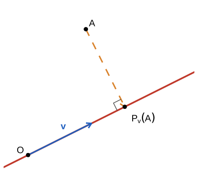
fig_7_6. Reproduces Holmes and Huber (2019), Figure 7.6. Download: PDF · SVG7.3.1 Lower-dimensional projections
The simplest way to reduce two variables to one is to keep one of them, i.e. to project every point onto a coordinate axis (Figure 7.7). For the standardised discus and shot put ("weight") results the projected points on the horizontal axis have variance 1, the variance of the weight variable, and all information about the discus is lost. The projection onto the vertical axis likewise has variance 1 (the book's Task).
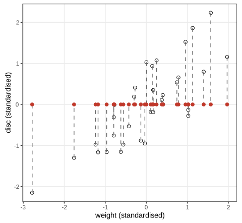
fig_7_7. Reproduces Holmes and Huber (2019), Figure 7.7. Download: PDF · SVGFilling the gap 7.3: orthogonal projection onto a line, and the variance of projected points Section 7.3, Figures 7.6, 7.7
The book defines projections by a picture. Here is the formula and the two facts used throughout the chapter.
Derivation
Let \(\mathbf{v}\ne\mathbf{0}\) span a line through the origin and \(\mathbf{a}\) be a point. The points of the line are \(t\mathbf{v}\), and the squared distance \(f(t)=\|\mathbf{a}-t\mathbf{v}\|^2=\|\mathbf{a}\|^2-2t\,\mathbf{v}^\T\mathbf{a}+t^2\|\mathbf{v}\|^2\) is a convex quadratic in \(t\), minimised where \(f'(t)=0\):
\[ t^\ast=\frac{\mathbf{v}^\T\mathbf{a}}{\mathbf{v}^\T\mathbf{v}},\qquad P_{\mathbf{v}}(\mathbf{a})=\frac{\mathbf{v}^\T\mathbf{a}}{\mathbf{v}^\T\mathbf{v}}\,\mathbf{v}=\frac{\mathbf{v}\mathbf{v}^\T}{\mathbf{v}^\T\mathbf{v}}\,\mathbf{a}. \](i) Orthogonality. \(\mathbf{v}^\T(\mathbf{a}-P_{\mathbf{v}}\mathbf{a})=\mathbf{v}^\T\mathbf{a}-t^\ast\mathbf{v}^\T\mathbf{v}=0\), so the residual is perpendicular to the line, and by Pythagoras \(\|\mathbf{a}\|^2=\|P_{\mathbf{v}}\mathbf{a}\|^2+\|\mathbf{a}-P_{\mathbf{v}}\mathbf{a}\|^2\). The matrix \(\mathbf{P}=\mathbf{v}\mathbf{v}^\T/\mathbf{v}^\T\mathbf{v}\) is symmetric, idempotent and of rank one.
(ii) Variance of projected points. Take \(\|\mathbf{v}\|=1\) and project every centred observation \(\mathbf{x}_i\). The projection is \((\mathbf{v}^\T\mathbf{x}_i)\mathbf{v}\), so its position along the line is the number \(\mathbf{v}^\T\mathbf{x}_i\), the \(i\)th entry of \(\X\mathbf{v}\). By Filling the gap 7.1 these coordinates have variance \(\mathbf{v}^\T\Sh\mathbf{v}\). For the horizontal axis \(\mathbf{v}=\mathbf{e}_1\) and the variance is \(S_{11}\), the variance of the first variable. ∎
7.3.2 How do we summarize two-dimensional data by a line?
Regression gives two candidate lines. Regressing discus on weight minimises the squared vertical distances to the line (Figure 7.8); regressing weight on discus minimises the squared horizontal distances (Figure 7.9). Both are supervised: one variable is treated as the response.
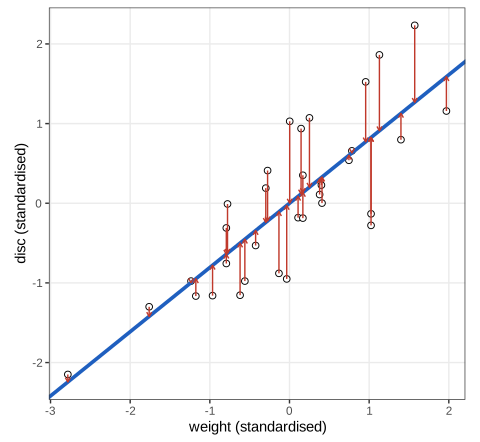
fig_7_8. Reproduces Holmes and Huber (2019), Figure 7.8. Download: PDF · SVG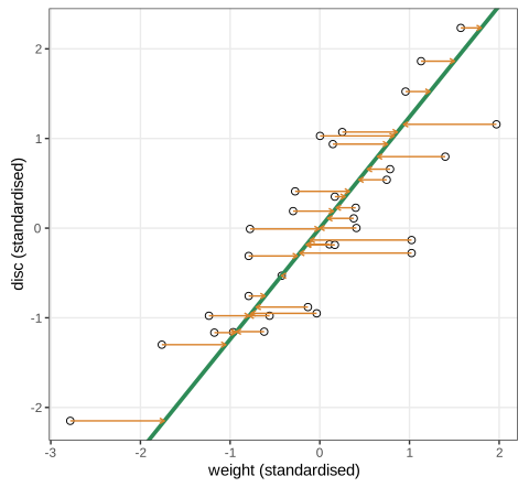
fig_7_9. Reproduces Holmes and Huber (2019), Figure 7.9. Download: PDF · SVGFilling the gap 7.4: regression is an orthogonal projection, and Question 7.6 Section 7.3.2, Question 7.6
The book fits the two lines with lm and answers Question 7.6 with "Pythagoras' theorem". Here is the argument in full.
Derivation
The least-squares line. Minimise \(Q(\beta_0,\beta_1)=\sum_i(y_i-\beta_0-\beta_1x_i)^2\). Setting both partial derivatives to zero gives the normal equations \(\sum_i(y_i-\beta_0-\beta_1x_i)=0\) and \(\sum_ix_i(y_i-\beta_0-\beta_1x_i)=0\). The first gives \(\hat\beta_0=\bar y-\hat\beta_1\bar x\) (the line passes through \((\bar x,\bar y)\)); substituting into the second,
\[ \hat\beta_1=\frac{\sum_i(x_i-\bar x)(y_i-\bar y)}{\sum_i(x_i-\bar x)^2}=\frac{s_{xy}}{s_x^2}=r\,\frac{s_y}{s_x}. \]\(Q\) is a convex quadratic whose Hessian \(2\begin{pmatrix}n&\sum x_i\\ \sum x_i&\sum x_i^2\end{pmatrix}\) has determinant \(4n\sum_i(x_i-\bar x)^2>0\) when the \(x_i\) are not all equal, so this stationary point is the unique minimum. For standardised variables \(s_x=s_y=1\) and the slope is \(r\).
Fitted values are a projection. With the \(n\times2\) design matrix \(\mathbf{A}=[\one,\mathbf{x}]\), the normal equations read \(\mathbf{A}^\T(\mathbf{y}-\mathbf{A}\hat{\bm\beta})=\mathbf{0}\), so the residual \(\mathbf{e}=\mathbf{y}-\hat{\mathbf{y}}\) is orthogonal to \(\one\) and to \(\mathbf{x}\), and \(\hat{\mathbf{y}}=\mathbf{A}(\mathbf{A}^\T\mathbf{A})^{-1}\mathbf{A}^\T\mathbf{y}\) is the orthogonal projection of \(\mathbf{y}\) onto the plane \(\spn\{\one,\mathbf{x}\}\subset\R^n\). Because \(\mathbf{e}\perp\one\), the residuals have mean zero, and because \(\hat{\mathbf{y}}-\bar y\one\) lies in the plane, Pythagoras in \(\R^n\) gives
\[ \|\mathbf{y}-\bar y\one\|^2=\|\hat{\mathbf{y}}-\bar y\one\|^2+\|\mathbf{e}\|^2,\qquad\text{i.e.}\quad \var(\mathbf{y})=\var(\hat{\mathbf{y}})+\var(\mathbf{e}), \]with \(\var(\hat{\mathbf{y}})=\hat\beta_1^2s_x^2=r^2s_y^2\): a fraction \(r^2\) of the variance of \(\mathbf{y}\) is explained.
Question 7.6. The feet of the red arrows in Figure 7.8 are the points \((x_i,\hat y_i)\) on the blue line. Their total variance in the plane is the sum of the variances of their two coordinates,
\[ \var(\mathbf{x})+\var(\hat{\mathbf{y}})=1+r^2=1+0.8064^2=1.650 \]for the standardised data. Note that these are vertical projections onto the line, not orthogonal ones, which is why the answer differs from the variance along the principal component line found next. ∎
The line that treats both variables alike minimises the squared perpendicular distances: the first principal component line (Figure 7.10). Figure 7.11 shows all three.
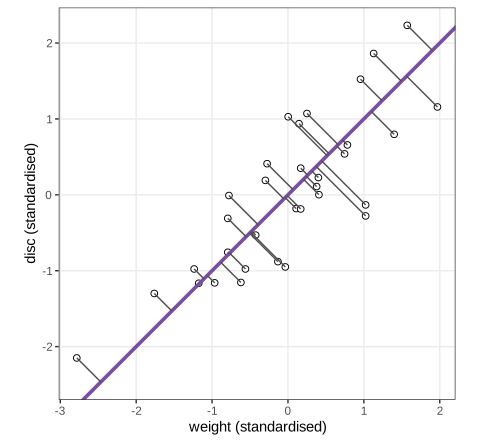
fig_7_10. Reproduces Holmes and Huber (2019), Figure 7.10. Download: PDF · SVG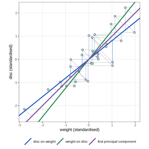
fig_7_11. Reproduces Holmes and Huber (2019), Figure 7.11. Download: PDF · SVGFilling the gap 7.5: the principal component line of two variables (Questions 7.7 and 7.8) Section 7.3.2, Figures 7.10, 7.11
The book observes that the purple line is the diagonal, that its slope lies between the regression slopes, and that the projected points have variance 1.81. All three facts follow from a 2 × 2 eigenvalue problem.
Derivation
Variance along a direction. For standardised variables with correlation \(r\), \(\Sh=\Rm=\begin{pmatrix}1&r\\ r&1\end{pmatrix}\). A unit direction is \(\mathbf{a}=(\cos\theta,\sin\theta)^\T\), and by Filling the gap 7.3 the projected points have variance
\[ \mathbf{a}^\T\Rm\mathbf{a}=\cos^2\theta+2r\cos\theta\sin\theta+\sin^2\theta=1+r\sin2\theta. \]For \(r>0\) this is largest at \(\theta=45^\circ\), with value \(1+r\), and smallest at \(\theta=135^\circ\), with value \(1-r\) (for \(r<0\) the roles swap). Equivalently, \(\Rm(1,1)^\T=(1+r)(1,1)^\T\) and \(\Rm(1,-1)^\T=(1-r)(1,-1)^\T\): the eigenvalues of a 2 × 2 correlation matrix are \(1\pm r\) and its eigenvectors are the two diagonals, whatever the value of \(r\). That is why the purple line has slope exactly 1 (Question 7.7) and why svd returns the loadings \(\pm(0.707,0.707)\).
The inertia decomposition. Let \(\mathbf{b}=(-\sin\theta,\cos\theta)^\T\) be the unit normal. For each centred point Pythagoras gives \(\|\mathbf{x}_i\|^2=(\mathbf{a}^\T\mathbf{x}_i)^2+(\mathbf{b}^\T\mathbf{x}_i)^2\), the squared position along the line plus the squared distance to it. Summing and dividing by \(n-1\):
\[ \underbrace{\Tr\Sh}_{\text{total variance (inertia)}}=\underbrace{\mathbf{a}^\T\Sh\mathbf{a}}_{\text{variance along}}+\underbrace{\tfrac{1}{n-1}\textstyle\sum_i(\mathbf{b}^\T\mathbf{x}_i)^2}_{\text{mean squared distance}}. \]The left side does not depend on \(\theta\), so minimising the perpendicular distances is the same as maximising the variance along the line. This holds for any \(\Sh\), not only for standardised data.
Question 7.8. The orthogonal projections have coordinates \((\mathbf{a}^\T\mathbf{x}_i)\mathbf{a}\) with \(\mathbf{a}=(1,1)/\sqrt2\), so each coordinate has variance \((1+r)/2=0.903\), and their sum is \(1+r=1.806\), larger than the 1.650 of Question 7.6 and the 1 of either axis.
Unstandardised data and the ordering of slopes. For a general \(\Sh=\begin{pmatrix}s_x^2&s_{xy}\\ s_{xy}&s_y^2\end{pmatrix}\) with \(s_{xy}>0\), the leading eigenvalue \(\lambda_1\) solves \((\lambda-s_x^2)(\lambda-s_y^2)=s_{xy}^2\), and the eigenvector \((1,b)\) has slope \(b_{\rm PC}=(\lambda_1-s_x^2)/s_{xy}\). Put \(u=\lambda_1-s_x^2\); \(u\ge0\) because \(\lambda_1\ge\mathbf{e}_1^\T\Sh\mathbf{e}_1=s_x^2\). The characteristic equation gives \(s_{xy}^2/u=\lambda_1-s_y^2\), and \(\lambda_1\le\lambda_1+\lambda_2=s_x^2+s_y^2\) because \(\lambda_2\ge0\). Hence
\[ \frac{s_{xy}}{s_x^2}\ \le\ b_{\rm PC}=\frac{u}{s_{xy}}\ \le\ \frac{s_y^2}{s_{xy}}, \]the left inequality being \(s_{xy}^2/u=\lambda_1-s_y^2\le s_x^2\) and the right one \(u\le s_y^2\). The left bound is the slope of \(y\) on \(x\), the right bound the slope of the line of \(x\) on \(y\) drawn in the same plane: the principal component line always lies between the two regression lines. Unlike them it depends on the units: rescaling \(y\) by \(c\) multiplies \(s_y^2\) by \(c^2\), and as \(c\to\infty\) the principal component line turns towards the \(y\) axis (Question 7.7, second part). ∎
The ordering of slopes, \(r<1<1/r\), is the geometry of regression to the mean: predicting one standardised variable from the other always shrinks towards zero by the factor \(r\), in either direction, so neither regression line can be the symmetric summary.
7.4 The new linear combinations
A principal component is a new variable built as a linear combination of the old ones; its coefficients are the loadings, like the amounts in a juice recipe (Question 7.9: the calories of a glass are the same linear combination of the calories per unit of each ingredient). The book writes the purple line of Figure 7.10 as
\[ PC=\tfrac12\,\text{disc}+\tfrac12\,\text{weight}. \tag{7.2} \]Note on (7.2)
The coefficients \(\tfrac12,\tfrac12\) give the coordinates of the projected points, \(((d+w)/2,(d+w)/2)\), but they do not form a unit vector. As a principal component, i.e. the position of each athlete along the line, the score is \(PC_1=(\text{disc}+\text{weight})/\sqrt2\), with loadings \(0.707\), as the book itself states in Section 7.7 (up to the arbitrary sign). The scaling matters: with loadings \(\tfrac12\) the variance would be \((1+r)/2\), not the eigenvalue \(1+r\).
Definition 7.2 (loadings, principal components, scores) Sections 7.4, 7.6.4
Let \(\X\) be centred (and possibly scaled). A loading vector is a unit vector \(\mathbf{v}\in\R^p\); the corresponding principal component is the new variable \(\mathbf{z}=\X\mathbf{v}=\sum_jv_j\mathbf{x}_{\cdot j}\), whose \(n\) entries are the scores of the observations. The first principal component uses the loading vector that maximises \(\var(\X\mathbf{v})\); the \(k\)th maximises it among unit vectors orthogonal to the first \(k-1\) loading vectors (Result 7.5).
7.4.1 Optimal lines
The book's argument for maximising variance is visual (Figures 7.12 and 7.14, two shadows of the same object, not reproduced): the projection that spreads the points most shows the most. The inertia decomposition of Filling the gap 7.5 makes this precise in any dimension and also says where the best line or plane must pass.
Filling the gap 7.6: the best-fitting affine subspace passes through the centroid (Pearson's problem) Section 7.4.1
The book takes for granted that the line passes through the centre of gravity and that "minimising the distances" equals "maximising the variance". Both hold for a best-fitting subspace of any dimension \(k\).
Derivation
An affine subspace of dimension \(k\) is \(\{\mathbf{m}+\Q\mathbf{t}:\mathbf{t}\in\R^k\}\), with \(\Q\in\R^{p\times k}\) having orthonormal columns (\(\Q^\T\Q=\I_k\)). By Filling the gap 7.3 applied to a subspace (the closest point is the orthogonal projection, \(\mathbf{P}=\Q\Q^\T\)), the squared distance of \(\mathbf{x}_i\) to it is \(\|(\I-\Q\Q^\T)(\mathbf{x}_i-\mathbf{m})\|^2\). Write \(\mathbf{M}=\I-\Q\Q^\T\) (symmetric, idempotent). For fixed \(\Q\), the gradient of \(\sum_i\|\mathbf{M}(\mathbf{x}_i-\mathbf{m})\|^2\) in \(\mathbf{m}\) is \(-2\mathbf{M}\sum_i(\mathbf{x}_i-\mathbf{m})\), which vanishes at \(\mathbf{m}=\bar{\mathbf{x}}\); the function is convex in \(\mathbf{m}\), so \(\bar{\mathbf{x}}\) is a minimiser (any \(\mathbf{m}\) differing from it by an element of \(\spn\Q\) describes the same subspace). So the optimal subspace passes through the centroid.
With centred data, \(\|\mathbf{M}\mathbf{x}_i\|^2=\|\mathbf{x}_i\|^2-\|\Q^\T\mathbf{x}_i\|^2\) by Pythagoras, and summing over \(i\),
\[ \sum_i\operatorname{dist}(\mathbf{x}_i,\text{subspace})^2=(n-1)\big[\Tr\Sh-\Tr(\Q^\T\Sh\Q)\big]. \]\(\Tr(\Q^\T\Sh\Q)=\sum_{m=1}^k\mathbf{q}_m^\T\Sh\mathbf{q}_m\) is the total variance of the projected points. Minimising the distances is therefore the same as maximising the projected variance, and Filling the gap 7.9 (step 3) shows that the maximum is the sum of the \(k\) largest eigenvalues of \(\Sh\), attained when \(\Q\) holds the corresponding eigenvectors. This is Pearson's (1901) solution. ∎
Question 7.11. The projection with the larger "shadow", i.e. the larger spread of the projected points, typically shows more of the object's structure; PCA chooses that perspective.
7.5 The PCA workflow
The book summarises the workflow in a diagram (Figure 7.13, not reproduced). In words:
Algorithm 7.1 (a principal component analysis) Section 7.5, Figure 7.13
- Look at the variables one and two at a time: histograms, scatterplots, the correlation matrix.
- Centre the columns. Decide whether to scale them: correlation PCA (standardised variables) when units differ or are arbitrary, covariance PCA (centred only) when all variables share a unit whose spreads are meaningful.
- Compute the SVD of the preprocessed matrix, \(\X=\U\Sm\V^\T\) (Theorem 7.3). The loadings are the columns of \(\V\), the scores \(\U\Sm=\X\V\), the variances \(\lambda_k=s_k^2/(n-1)\) (Theorem 7.6).
- Draw the scree plot of the \(\lambda_k\) (or their percentages) and choose the rank \(k\) (Section 7.7.3).
- Plot the observations in the principal plane (scores), the variables in the correlation circle, or both in a biplot; add supplementary information (groups, extra variables) to interpret the axes.
Step 2 is not a formality: the two choices give different axes.
Filling the gap 7.15: why scaling changes the principal components Sections 7.2.2, 7.5; Question 7.21
The book notes that functions differ in whether they scale by default (Question 7.21) and asks what happens without scaling. The answer: the axes change, because eigenvectors do not follow rescalings.
Derivation
Rescaling the variables by \(\B=\diag(b_j)\), \(b_j>0\), turns the covariance \(\Sh\) into \(\B\Sh\B\) (Filling the gap 7.2). If \(\Sh\mathbf{v}=\lambda\mathbf{v}\), then \(\B\Sh\B(\B^{-1}\mathbf{v})=\lambda\B\mathbf{v}\), which is not a multiple of \(\B^{-1}\mathbf{v}\) unless \(\B\) is a multiple of the identity on the relevant coordinates. So the eigenvectors of the rescaled covariance are not the rescaled eigenvectors: covariance PCA is not equivariant under changes of units. Correlation PCA is invariant, because \(\Rm\) does not change (Filling the gap 7.2).
A limiting case. Take two variables and multiply the second by \(c\): \(\Sh_c=\begin{pmatrix}s_1^2&cs_{12}\\ cs_{12}&c^2s_2^2\end{pmatrix}\). Dividing by \(c^2\), \(\Sh_c/c^2\to\begin{pmatrix}0&0\\0&s_2^2\end{pmatrix}\) as \(c\to\infty\), whose leading eigenvector is \(\mathbf{e}_2\); eigenvectors of a symmetric matrix with a simple top eigenvalue depend continuously on its entries, so the first principal component converges to the second variable. Whatever variable has the largest variance in its own units takes over the first axis.
The decathlon in raw units. The 1500 m time has variance 186.5 s\(^2\), the javelin 30.2 m\(^2\), the 100 m 0.06 s\(^2\). Covariance PCA of the raw data puts 81.2% of the "variance" on the first component, whose loading on the 1500 m is 0.990: the first axis is simply the 1500 m time, a statement about the choice of seconds as a unit, not about athletes. ∎
7.6 The inner workings of PCA: rank reduction
The book now opens the box: the computation behind PCA is the singular value decomposition, which writes a matrix as a sum of simple "rectangular" pieces. It builds the idea from matrices that are a single such piece.
7.6.1 Rank-one matrices
Multiplying a column \(\mathbf{u}\in\R^n\) by a row \(\mathbf{v}^\T\) (\(\mathbf{v}\in\R^p\)) gives the \(n\times p\) matrix \(\mathbf{u}\mathbf{v}^\T\) with entries \(u_iv_j\). With \(\mathbf{u}=(1,2,3,4)^\T\) and \(\mathbf{v}=(2,4,8)^\T\),
\[ \X=\begin{pmatrix}2&4&8\\ 4&8&16\\ 6&12&24\\ 8&16&32\end{pmatrix}=\mathbf{u}\mathbf{v}^\T. \tag{7.3} \]Twelve numbers are described by seven (Question 7.12: \(n+p\) instead of \(np\), a saving that grows with the size). The book's matrix
\[ \X=\begin{pmatrix}780&936&1300&728\\ 75&90&125&70\\ 540&648&900&504\end{pmatrix} \tag{7.4} \]is of the same kind (Question 7.13): with \(\mathbf{u}=(52,5,36)^\T\) and \(\mathbf{v}=(15,18,25,14)^\T\), every entry is \(u_iv_j\). Drawing each cell as a rectangle with sides \(u_i\) and \(v_j\) makes the structure visible (Figures 7.15 and 7.16).
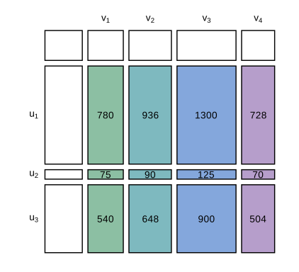
fig_7_15. Reproduces Holmes and Huber (2019), Figure 7.15. Download: PDF · SVG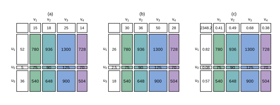
fig_7_16. Reproduces Holmes and Huber (2019), Figure 7.16. Download: PDF · SVGDefinition 7.3 (rank) Sections 7.6.1, 7.6.2
The rank of a matrix is the dimension of the space spanned by its columns (equivalently, by its rows). A matrix has rank one exactly when it is nonzero and all its columns are multiples of one vector.
Result 7.1 (rank-one matrices and their normalised form) Section 7.6.1, Figure 7.16, Exercise 7.1
(a) \(\X\in\R^{n\times p}\) has rank one if and only if \(\X=\mathbf{u}\mathbf{v}^\T\) for some nonzero \(\mathbf{u},\mathbf{v}\). (b) The factors are not unique: \(\mathbf{u}\mathbf{v}^\T=(c\mathbf{u})(\mathbf{v}/c)^\T\) for every \(c\ne0\). (c) Requiring \(\|\mathbf{u}\|=\|\mathbf{v}\|=1\) and writing \(\X=s\,\mathbf{u}\mathbf{v}^\T\) with \(s>0\) makes the decomposition unique up to the joint sign change \((\mathbf{u},\mathbf{v})\to(-\mathbf{u},-\mathbf{v})\), and then \(s=\|\X\|_\F\).
Filling the gap 7.7: proof of Result 7.1 Section 7.6.1
The book shows non-uniqueness with pictures and then fixes the norms "to make the choice unique". Here is why that works, and what is still free.
Proof
(a) If \(\X=\mathbf{u}\mathbf{v}^\T\) with nonzero factors, column \(j\) is \(v_j\mathbf{u}\), so all columns lie on the line spanned by \(\mathbf{u}\), and some \(v_j\ne0\) makes \(\X\ne\mathbf{0}\): rank one. Conversely, if the column space is spanned by one vector \(\mathbf{u}\ne\mathbf{0}\), each column is \(\mathbf{x}_{\cdot j}=v_j\mathbf{u}\) for some number \(v_j\); collecting these numbers into \(\mathbf{v}\) gives \(\X=\mathbf{u}\mathbf{v}^\T\), with \(\mathbf{v}\ne\mathbf{0}\) because \(\X\ne\mathbf{0}\).
(b) is immediate. (c) Existence: put \(s=\|\mathbf{u}\|\|\mathbf{v}\|\) and use \(\mathbf{u}/\|\mathbf{u}\|\), \(\mathbf{v}/\|\mathbf{v}\|\). For uniqueness, suppose \(s\mathbf{u}\mathbf{v}^\T=s'\mathbf{u}'\mathbf{v}'^\T\) with unit vectors. The column spaces agree, so \(\mathbf{u}'=\pm\mathbf{u}\); the row spaces agree, so \(\mathbf{v}'=\pm\mathbf{v}\). Taking Frobenius norms, \(\|\mathbf{u}\mathbf{v}^\T\|_\F^2=\sum_{ij}u_i^2v_j^2=\|\mathbf{u}\|^2\|\mathbf{v}\|^2=1\), so \(s=s'=\|\X\|_\F\), and then the two signs must agree. For (7.4), \(\|\X\|_\F=2348.24\), \(\mathbf{u}=(0.8196,0.0788,0.5674)\) and \(\mathbf{v}=(0.4053,0.4863,0.6754,0.3782)\), the values of Question 7.14 and Figure 7.16(c). ∎
Question 7.14. svd(X) returns d (singular values), u and v (singular vectors, unit-norm columns). The value \(s_1=2348.2\) is svd(X)$d[1]; the other two singular values are of order \(10^{-13}\), zero up to rounding, which is the numerical signature of rank one.
7.6.2 How do we find such a decomposition in a unique way?
Most matrices are not rank one, but every matrix is a sum of rank-one pieces. For the book's 5 × 4 matrix Xtwo the singular values are \(135.06,\ 28.05,\ 4.1\times10^{-15},\ 2.7\times10^{-16}\) (Question 7.15). Subtracting the first piece \(s_1\mathbf{u}_1\mathbf{v}_1^\T\) leaves a residual with entries up to 19; subtracting the second as well leaves entries of order \(10^{-14}\) (Question 7.16). So Xtwo has rank two. To make the pieces unique the SVD asks, besides unit norms, that the \(\mathbf{u}\)'s be mutually orthogonal and the \(\mathbf{v}\)'s too; the Task checks that t(USV$u) %*% USV$u and t(USV$v) %*% USV$v are identity matrices. Orthogonality is what makes the squared sizes of the pieces add up.
Result 7.2 (Pythagoras for orthogonal rank-one pieces)
If \(\mathbf{u}_1,\dots,\mathbf{u}_r\) are orthonormal and \(\mathbf{v}_1,\dots,\mathbf{v}_r\) are orthonormal, then \(\big\|\sum_ks_k\mathbf{u}_k\mathbf{v}_k^\T\big\|_\F^2=\sum_ks_k^2\).
Proof
\(\|\mathbf{A}\|_\F^2=\Tr(\mathbf{A}^\T\mathbf{A})\). With \(\mathbf{A}=\sum_ks_k\mathbf{u}_k\mathbf{v}_k^\T\), \(\mathbf{A}^\T\mathbf{A}=\sum_{k,l}s_ks_l\mathbf{v}_k(\mathbf{u}_k^\T\mathbf{u}_l)\mathbf{v}_l^\T=\sum_ks_k^2\mathbf{v}_k\mathbf{v}_k^\T\), and \(\Tr(\mathbf{v}_k\mathbf{v}_k^\T)=\mathbf{v}_k^\T\mathbf{v}_k=1\). ∎
The turtles. The SVD of the standardised turtle matrix (48 × 3) has singular values \(11.746,\ 1.419,\ 1.003\) and first right singular vector \((0.579,0.578,0.575)\) (Question 7.17). The three loadings are nearly equal, close to (but not exactly) \(\sqrt{1/3}=0.577\): the first component is essentially the average size. And \(\sum_ks_k^2/47=3\) exactly: by Result 7.2 this is \(\|\X\|_\F^2/(n-1)\), the sum of the three column variances, each equal to one after standardisation (Filling the gap 7.1).
7.6.3 Singular value decomposition
Definition 7.4 (singular value decomposition) Section 7.6.3, (7.5)
A singular value decomposition of \(\X\in\R^{n\times p}\) of rank \(r\) is
\[ \X=\U\Sm\V^\T,\qquad \V^\T\V=\I,\quad \U^\T\U=\I, \tag{7.5} \]with \(\U\in\R^{n\times r}\), \(\V\in\R^{p\times r}\) and \(\Sm=\diag(s_1,\dots,s_r)\), \(s_1\ge\dots\ge s_r>0\). Entrywise, \(x_{ij}=\sum_{k=1}^r u_{ik}s_kv_{jk}\): a sum of \(r\) rank-one pieces \(s_k\mathbf{u}_k\mathbf{v}_k^\T\). The \(s_k\) are the singular values, the columns \(\mathbf{u}_k\), \(\mathbf{v}_k\) the left and right singular vectors. (R's svd returns the "thin" version with \(\min(n,p)\) columns, padding with zero singular values; the full version extends \(\U,\V\) to square orthogonal matrices.)
Theorem 7.3 (existence and uniqueness of the SVD) Section 7.6.3
Every real matrix has a singular value decomposition. The singular values are unique: \(s_k^2\) are the nonzero eigenvalues of \(\X^\T\X\) (and of \(\X\X^\T\)). If the \(s_k\) are distinct, each pair \((\mathbf{u}_k,\mathbf{v}_k)\) is unique up to a joint change of sign. The rank of \(\X\) equals the number of nonzero singular values.
Filling the gap 7.8: proof of Theorem 7.3 Section 7.6.3
The book calls svd and observes its properties. The proof constructs the decomposition from the spectral theorem for the symmetric matrix \(\X^\T\X\).
Proof
Step 1 (the eigenproblem). \(\X^\T\X\) is symmetric and positive semi-definite, since \(\mathbf{a}^\T\X^\T\X\mathbf{a}=\|\X\mathbf{a}\|^2\ge0\). By the spectral theorem \(\X^\T\X=\sum_{k=1}^p\lambda_k\mathbf{v}_k\mathbf{v}_k^\T\) with orthonormal \(\mathbf{v}_1,\dots,\mathbf{v}_p\) and \(\lambda_1\ge\dots\ge\lambda_p\ge0\).
Step 2 (the rank). \(\X^\T\X\) and \(\X\) have the same null space: \(\X\mathbf{a}=\mathbf{0}\) gives \(\X^\T\X\mathbf{a}=\mathbf{0}\), and \(\X^\T\X\mathbf{a}=\mathbf{0}\) gives \(\|\X\mathbf{a}\|^2=\mathbf{a}^\T\X^\T\X\mathbf{a}=0\). So both have rank \(r\), and exactly \(\lambda_1,\dots,\lambda_r\) are positive.
Step 3 (the left vectors). For \(k\le r\) put \(s_k=\sqrt{\lambda_k}\) and \(\mathbf{u}_k=\X\mathbf{v}_k/s_k\). These are orthonormal:
\[ \mathbf{u}_k^\T\mathbf{u}_l=\frac{\mathbf{v}_k^\T\X^\T\X\mathbf{v}_l}{s_ks_l}=\frac{\lambda_l\,\mathbf{v}_k^\T\mathbf{v}_l}{s_ks_l}=\delta_{kl}. \]For \(k>r\), \(\|\X\mathbf{v}_k\|^2=\lambda_k=0\), so \(\X\mathbf{v}_k=\mathbf{0}\).
Step 4 (assembly). Since \(\sum_{k=1}^p\mathbf{v}_k\mathbf{v}_k^\T=\I\) (orthonormal basis),
\[ \X=\X\sum_{k=1}^p\mathbf{v}_k\mathbf{v}_k^\T=\sum_{k=1}^r(\X\mathbf{v}_k)\mathbf{v}_k^\T=\sum_{k=1}^rs_k\mathbf{u}_k\mathbf{v}_k^\T=\U\Sm\V^\T. \]Uniqueness. From any SVD, \(\X^\T\X=\V\Sm\U^\T\U\Sm\V^\T=\V\Sm^2\V^\T\) and \(\X\X^\T=\U\Sm^2\U^\T\), so the \(s_k^2\) are the nonzero eigenvalues of both, which are unique, and the rank statement follows from Step 2. If the \(s_k\) are distinct, each eigenspace of \(\X^\T\X\) is a line, so \(\mathbf{v}_k\) is unique up to sign, and \(\mathbf{u}_k=\X\mathbf{v}_k/s_k\) follows it. If \(s_k=s_{k+1}\), any rotation of \((\mathbf{v}_k,\mathbf{v}_{k+1})\) within their plane, applied to the \(\mathbf{u}\)'s as well, gives another SVD; this is the source of the instability discussed in Section 7.7.3. Finally \(\X^\T\mathbf{u}_k=s_k\mathbf{v}_k\) and \(\X\mathbf{v}_k=s_k\mathbf{u}_k\): each singular vector is mapped onto its partner. ∎
In floating point. "Zero" singular values come out as tiny numbers (\(4\times10^{-15}\) for Xtwo); the numerical rank counts the singular values above a tolerance such as \(10^{-10}s_1\).
Truncating the sum after \(k\) terms gives a matrix of rank \(k\). The fact that makes PCA work is that this truncation is the best approximation of rank \(k\); the book uses it throughout ("this decomposition provides a lower rank approximation") without stating it.
Theorem 7.4 (Eckart–Young–Mirsky) Sections 7.6.3, 7.9
Let \(\X=\sum_{j=1}^rs_j\mathbf{u}_j\mathbf{v}_j^\T\) and, for \(k<r\), \(\X_k=\sum_{j=1}^ks_j\mathbf{u}_j\mathbf{v}_j^\T\). For every matrix \(\B\) of rank at most \(k\),
\[ \|\X-\B\|_\F^2\ \ge\ \|\X-\X_k\|_\F^2=\sum_{j=k+1}^rs_j^2,\qquad \|\X-\B\|_2\ \ge\ \|\X-\X_k\|_2=s_{k+1}. \]If \(s_k>s_{k+1}\), \(\X_k\) is the unique minimiser in the Frobenius norm. (Eckart and Young 1936 for the Frobenius norm; Mirsky 1960 for all unitarily invariant norms.)
Filling the gap 7.9: proof of the Eckart–Young–Mirsky theorem Section 7.6.3
The proof needs only orthogonal projection (Filling the gap 7.3) and a one-line exchange argument (Ky Fan's maximum principle).
Proof
Step 0 (the error of the truncation). \(\X-\X_k=\sum_{j>k}s_j\mathbf{u}_j\mathbf{v}_j^\T\), so by Result 7.2 \(\|\X-\X_k\|_\F^2=\sum_{j>k}s_j^2\). For the spectral norm, a unit \(\mathbf{w}=\sum_jc_j\mathbf{v}_j+\mathbf{w}_\perp\) (with \(\mathbf{w}_\perp\) orthogonal to all \(\mathbf{v}_j\)) gives \(\|(\X-\X_k)\mathbf{w}\|^2=\sum_{j>k}s_j^2c_j^2\le s_{k+1}^2\), with equality at \(\mathbf{w}=\mathbf{v}_{k+1}\).
Step 1 (fix the column space). Let \(\rank\B\le k\). Its columns lie in a subspace of dimension \(k\) with an orthonormal basis \(\Q\in\R^{n\times k}\) (enlarge the column space if its dimension is below \(k\)), so \(\B=\Q\Cs\) for some \(\Cs\). Column by column, \(\|\mathbf{x}_{\cdot j}-\Q\mathbf{c}_j\|\ge\|\mathbf{x}_{\cdot j}-\Q\Q^\T\mathbf{x}_{\cdot j}\|\), because the orthogonal projection is the closest point of the subspace. Hence, using Pythagoras for each column,
\[ \|\X-\B\|_\F^2\ \ge\ \|(\I-\Q\Q^\T)\X\|_\F^2=\|\X\|_\F^2-\|\Q^\T\X\|_\F^2. \]Step 2 (rewrite the kept part). Complete \(\mathbf{u}_1,\dots,\mathbf{u}_r\) to an orthonormal basis \(\mathbf{u}_1,\dots,\mathbf{u}_n\) of \(\R^n\) and set \(s_j=0\) for \(j>r\). Then \(\X\X^\T=\sum_js_j^2\mathbf{u}_j\mathbf{u}_j^\T\) and
\[ \|\Q^\T\X\|_\F^2=\Tr(\Q^\T\X\X^\T\Q)=\sum_{j=1}^ns_j^2h_j,\qquad h_j=\|\Q^\T\mathbf{u}_j\|^2. \]Each \(h_j\) lies in \([0,1]\) (the projection \(\Q\Q^\T\) cannot lengthen a unit vector: \(h_j=\mathbf{u}_j^\T\Q\Q^\T\mathbf{u}_j=\|\Q\Q^\T\mathbf{u}_j\|^2\le1\)), and \(\sum_jh_j=\|\Q^\T\U_{\rm full}\|_\F^2=\|\Q\|_\F^2=k\) because \(\U_{\rm full}\) is orthogonal.
Step 3 (Ky Fan's bound). With \(s_1^2\ge s_2^2\ge\dots\),
\[ \sum_{j\le k}s_j^2-\sum_js_j^2h_j=\sum_{j\le k}s_j^2(1-h_j)-\sum_{j>k}s_j^2h_j\ \ge\ s_k^2\Big(\sum_{j\le k}(1-h_j)-\sum_{j>k}h_j\Big)=s_k^2\Big(k-\sum_jh_j\Big)=0, \]using \(1-h_j\ge0\), \(s_j^2\ge s_k^2\) for \(j\le k\), and \(h_j\ge0\), \(s_j^2\le s_k^2\) for \(j>k\). So \(\|\Q^\T\X\|_\F^2\le\sum_{j\le k}s_j^2\), and Step 1 gives \(\|\X-\B\|_\F^2\ge\sum_js_j^2-\sum_{j\le k}s_j^2=\sum_{j>k}s_j^2\). Equality needs equality in Step 3; when \(s_k>s_{k+1}\) that forces \(h_j=1\) for \(j\le k\), i.e. \(\spn\Q=\spn\{\mathbf{u}_1,\dots,\mathbf{u}_k\}\), and then Step 1 forces \(\B=\Q\Q^\T\X=\X_k\).
Spectral norm. The null space of \(\B\) has dimension at least \(p-k\) and \(\spn\{\mathbf{v}_1,\dots,\mathbf{v}_{k+1}\}\) has dimension \(k+1\), so they share a unit vector \(\mathbf{w}=\sum_{j\le k+1}c_j\mathbf{v}_j\). Then \(\|(\X-\B)\mathbf{w}\|^2=\|\X\mathbf{w}\|^2=\sum_{j\le k+1}s_j^2c_j^2\ge s_{k+1}^2\). ∎
Verification. For the standardised decathlon matrix (33 × 10) the rank-2 truncation has squared error 127.98; 3000 random rank-2 competitors (each the best matrix with a random column space) never got below 252.5, and a direct numerical minimisation over all rank-2 products \(\mathbf{A}\B^\T\) stopped at 127.98.
7.6.4 Principal components
The right singular vectors of the (centred, possibly scaled) data matrix give the loadings, \(Z_1=v_{11}\mathbf{x}_{\cdot1}+\dots+v_{p1}\mathbf{x}_{\cdot p}=\X\mathbf{v}_1\), and the new variables have decreasing variances. Question 7.18: the first principal component of the turtles can be computed as \(s_1\mathbf{u}_1\) or as \(\X\mathbf{v}_1\); they agree because \(\X\V=\U\Sm\V^\T\V=\U\Sm\) (the maximal difference in R is \(5\times10^{-15}\)). The book characterises the components by an optimisation problem, written informally as maximising the variance of the projection subject to orthogonality to previous components. Here it is with proof.
Result 7.5 (PCA as variance maximisation) Section 7.6.4
Let \(\Sh\) be the covariance matrix of the centred data, with eigenvalues \(\lambda_1\ge\dots\ge\lambda_p\ge0\) and orthonormal eigenvectors \(\mathbf{v}_1,\dots,\mathbf{v}_p\). Then
\[ \max_{\|\mathbf{a}\|=1}\var(\X\mathbf{a})=\lambda_1,\quad\text{attained at }\mathbf{a}=\mathbf{v}_1, \]and for \(k\ge2\), the maximum of \(\var(\X\mathbf{a})\) over unit vectors \(\mathbf{a}\) with \(\mathbf{a}\perp\mathbf{v}_1,\dots,\mathbf{v}_{k-1}\) is \(\lambda_k\), attained at \(\mathbf{v}_k\). Orthogonality of the loadings is equivalent to zero correlation between the components (when the earlier eigenvalues are positive).
Filling the gap 7.10: proof of Result 7.5 (Lagrange multipliers and the Rayleigh quotient) Section 7.6.4
The book states the maximisation property; it does not show why the answer is an eigenvector.
Proof
Lagrange. By Filling the gap 7.1, \(\var(\X\mathbf{a})=\mathbf{a}^\T\Sh\mathbf{a}\). Maximise it subject to \(g(\mathbf{a})=\mathbf{a}^\T\mathbf{a}-1=0\). The constraint gradient \(2\mathbf{a}\) never vanishes on the sphere, so at a maximiser \(\nabla(\mathbf{a}^\T\Sh\mathbf{a})=\lambda\nabla g\), i.e. \(2\Sh\mathbf{a}=2\lambda\mathbf{a}\): the stationary points are the unit eigenvectors, and at an eigenvector the objective equals its eigenvalue, \(\mathbf{a}^\T\Sh\mathbf{a}=\lambda\mathbf{a}^\T\mathbf{a}=\lambda\). The sphere is compact and the objective continuous, so a maximum exists, and it is the largest eigenvalue.
Without calculus (Rayleigh quotient). Expand \(\mathbf{a}=\sum_jc_j\mathbf{v}_j\); then \(\|\mathbf{a}\|^2=\sum_jc_j^2=1\) and
\[ \mathbf{a}^\T\Sh\mathbf{a}=\sum_j\lambda_jc_j^2\ \le\ \lambda_1\sum_jc_j^2=\lambda_1, \]with equality when all weight sits on eigenvectors with eigenvalue \(\lambda_1\). The constraint \(\mathbf{a}\perp\mathbf{v}_1,\dots,\mathbf{v}_{k-1}\) means \(c_1=\dots=c_{k-1}=0\), and the same bound gives \(\sum_{j\ge k}\lambda_jc_j^2\le\lambda_k\), attained at \(\mathbf{v}_k\).
Orthogonal loadings, uncorrelated components. \(\cov(\X\mathbf{a},\X\mathbf{v}_m)=\mathbf{a}^\T\Sh\mathbf{v}_m=\lambda_m\mathbf{a}^\T\mathbf{v}_m\), which is zero if and only if \(\mathbf{a}\perp\mathbf{v}_m\) when \(\lambda_m>0\). So "the \(k\)th component has maximal variance among those uncorrelated with the previous ones" and "among loadings orthogonal to the previous ones" are the same problem.
Second-order view. At \(\mathbf{v}_k\), moving along the sphere in the direction of another unit eigenvector \(\mathbf{v}_m\), \(\mathbf{a}(t)=\cos t\,\mathbf{v}_k+\sin t\,\mathbf{v}_m\), gives \(\mathbf{a}^\T\Sh\mathbf{a}=\lambda_k\cos^2t+\lambda_m\sin^2t\), which decreases if \(\lambda_m<\lambda_k\) and increases if \(\lambda_m>\lambda_k\). So only \(\mathbf{v}_1\) is a local maximum on the whole sphere; the other eigenvectors are saddle points, maxima only under their orthogonality constraints. ∎
The number of components is at most \(\min(n,p)\) (the book's first "useful fact"); for centred data it is at most \(\min(n-1,p)\), because centring removes one dimension (Filling the gap 7.1).
7.7 Plotting the observations in the principal plane
For two variables, PCA is a rotation of the plane that turns the first principal axis into the horizontal axis (Figure 7.17). For the standardised discus and weight results the loadings are \(\pm(0.707,0.707)\) (Question 7.19; the overall sign is arbitrary).
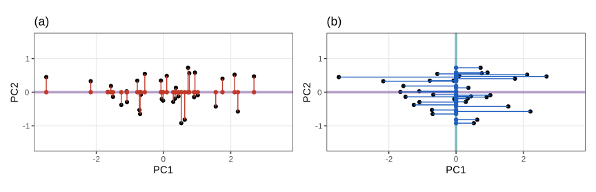
fig_7_17. Reproduces Holmes and Huber (2019), Figure 7.17. Download: PDF · SVGQuestion 7.20. The red segments in Figure 7.17(a) have lengths \(|\mathrm{PC2}_i|\), so their sum of squares is \(\sum_i s_2^2u_{i2}^2=s_2^2=6.20\); because the scores have mean zero, this equals \((n-1)\var(\mathrm{PC2})=32\times0.194\). The red points themselves have variance \(\var(\mathrm{PC1})=s_1^2/32=1.806\), larger by construction. The ratio of standard deviations is \(\mathrm{sd}(\mathrm{PC1})/\mathrm{sd}(\mathrm{PC2})=s_1/s_2=3.05\).
Theorem 7.6 (PCA from the SVD) Sections 7.6.4, 7.7.1
Let \(\X\) be the centred (possibly standardised) \(n\times p\) data matrix with SVD \(\X=\U\Sm\V^\T\), and \(\Sh=\X^\T\X/(n-1)\). Then (i) \(\Sh=\V\Lam\V^\T\) with \(\Lam=\Sm^2/(n-1)\): the loadings are the right singular vectors and the variances of the components are \(\lambda_k=s_k^2/(n-1)\); (ii) the scores are \(\Cs=\X\V=\U\Sm\), with column means zero, \(\Cs^\T\Cs=\Sm^2\), so the components are uncorrelated and \(\|\mathbf{c}_k\|^2=s_k^2\); (iii) \(\sum_k\lambda_k=\Tr\Sh=\sum_j\var(\mathbf{x}_{\cdot j})\), equal to \(p\) for standardised data.
Filling the gap 7.11: proof of Theorem 7.6, and the n versus n − 1 conventions (Questions 7.22, 7.23, 7.26, 7.27) Section 7.7.1
The book lists these facts ("Each principal component has a variance measured by the corresponding eigenvalue...") and warns that R functions use different conventions. Both are settled by the same three lines.
Proof
(i) \(\X^\T\X=\V\Sm\U^\T\U\Sm\V^\T=\V\Sm^2\V^\T\); divide by \(n-1\). This is the eigen-decomposition of \(\Sh\), and by Result 7.5 its eigenvectors are the loadings. (ii) \(\X\V=\U\Sm\V^\T\V=\U\Sm\). Since \(\one^\T\X=\mathbf{0}\) (centred columns), \(\one^\T\Cs=\mathbf{0}\); \(\Cs^\T\Cs=\Sm\U^\T\U\Sm=\Sm^2\) is diagonal, so the sample covariance of the scores is \(\Sm^2/(n-1)=\Lam\). The columns of \(\Cs\) are orthogonal with squared norms \(s_k^2\), not orthonormal (Question 7.23); the columns of \(\U\) are the normalised scores. (iii) \(\Tr\Sh=\Tr(\V\Lam\V^\T)=\Tr(\Lam\V^\T\V)=\sum_k\lambda_k\), and the trace is the sum of the variances, \(p\) after standardisation (Question 7.17: \(\sum_ks_k^2/47=3\)).
Conventions in R. prcomp reports \(\mathrm{sdev}^2=s_k^2/(n-1)\). princomp divides by \(n\): \(\mathrm{sdev}^2=s_k^2/n\). ade4::dudi.pca also uses \(1/n\) (uniform row weights \(1/n\)), but it re-standardises the columns with the divisor \(n\) as well; for already standardised input the two factors cancel, and its eigenvalues are those of the correlation matrix, \(s_k^2/(n-1)\) (Question 7.26: 2.9357, 0.0428, 0.0214, which are also the mean squared scores colSums(li^2)/48). The loadings are the same in all three up to sign.
Uncorrelated versus independent. The book adds that for normally distributed data uncorrelated components are independent. This is a statement about the population: if \(\mathbf{x}\sim\N(\bm\mu,\Sig)\) and \(\Sig=\bm\Gamma\Lam\bm\Gamma^\T\), then \(\bm\Gamma^\T(\mathbf{x}-\bm\mu)\sim\N(\mathbf{0},\Lam)\) has independent coordinates, because a Gaussian vector with diagonal covariance has independent coordinates. The sample scores are uncorrelated within the sample by construction (for any data, Gaussian or not), but they are not independent random variables: they are all computed with the same estimated \(\V\). ∎
Correction to Question 7.27
The book compares svd(scaledTurtles)$d / pcaturtles$sdev with sqrt(47) and explains the factor by implementations that "use \(1/(n-1)\)". In fact princomp uses \(1/n\): \(\mathrm{sdev}_k=s_k/\sqrt n\), so the ratio is \(\sqrt{48}=6.928\) for every component (checked numerically), not \(\sqrt{47}=6.856\). The general lesson stands: the two conventions differ by the factor \(n/(n-1)\) in the variances.
7.7.1 PCA of the turtles data
The standardised turtle data have correlations 0.96 to 0.98, and the first component carries 97.9% of the variance (Figure 7.18): the data are essentially one-dimensional. Its loadings \((0.579,0.578,0.575)\) weigh the three measurements equally, which is why this direction is called a size axis; the second component (1.4%) contrasts height with length and width, a shape axis (Jolicoeur and Mosimann 1960).
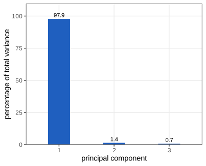
fig_7_18. Reproduces Holmes and Huber (2019), Figure 7.18. Download: PDF · SVGFilling the gap 7.12: the proportion of variance explained is a reconstruction error Sections 7.7.1, 7.7.3
The book advises annotating each axis with "the proportion of variance it explains". By Theorem 7.4 this number also measures how well \(k\) components reconstruct the whole data matrix.
Derivation
With \(\lambda_k=s_k^2/(n-1)\) and the truncation \(\X_k=\U_k\Sm_k\V_k^\T\) (scores times loadings of the first \(k\) components),
\[ \frac{\sum_{j\le k}\lambda_j}{\sum_j\lambda_j}=\frac{\sum_{j\le k}s_j^2}{\|\X\|_\F^2}=1-\frac{\|\X-\X_k\|_\F^2}{\|\X\|_\F^2}, \]by Result 7.2 and Step 0 of Filling the gap 7.9. So "the first \(k\) components explain 90% of the variance" means exactly that the best rank-\(k\) reconstruction leaves 10% of the total sum of squares. A scree plot is the plot of \(\lambda_k\) (or \(100\lambda_k/\sum\lambda_j\)) against \(k\). For correlation PCA the average eigenvalue is \(p/p=1\), and the rule of thumb "keep components with \(\lambda_k>1\)" (Kaiser 1960) keeps those that explain more than an average variable. ∎
Question 7.21 compares svd, prcomp, princomp and dudi.pca: on the standardised turtles all return the loadings \(\pm(0.579,0.578,0.575)\). Applied to the raw (unscaled) data, prcomp and princomp do covariance PCA by default and give different loadings (0.81, 0.49, 0.32 for length, width, height: length has the largest variance), while dudi.pca scales by default (Filling the gap 7.15). Question 7.22: scaledTurtles %*% res$loadings[, 1] equals res$scores[, 1], and \(\sqrt{\text{mean}(\text{scores}^2)}\) equals res$sdev[1] = 1.695 because princomp divides by \(n\).
A biplot shows the scores and the variables together (Figure 7.19). Females (orange) sit to the right, at larger sizes (Question 7.25a: the mean PC1 score is \(+1.04\) for females and \(-1.04\) for males); the three arrows point almost the same way, reflecting correlations close to one (Question 7.25b).
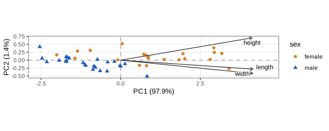
fig_7_19. Reproduces Holmes and Huber (2019), Figure 7.19. Download: PDF · SVGQuestion 7.24 asks whether a PCA plot with PC1 horizontal can be taller than wide. Since \(\lambda_1\ge\lambda_2\), the standard deviation along the first axis is always at least that along the second, and plots are typically wide. The range, which sets the plot's shape, can still be larger along the second axis: in the mass-spectrometry example of Section 7.8.1 the first-axis scores span 33.0 units and the second-axis scores 34.3, so an equal-scaled plot of Figure 7.30 is slightly taller than wide.
Question 7.26 is answered in Filling the gap 7.11. The variables are drawn in the correlation circle (Figure 7.20).
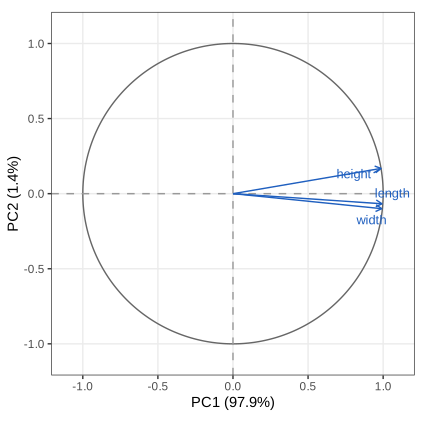
fig_7_20. Reproduces Holmes and Huber (2019), Figure 7.20. Download: PDF · SVGFilling the gap 7.13: why the arrows of a correlation circle are correlations, and what lengths and angles mean Section 7.7.1, Figures 7.20, 7.23
The book says that the angles between arrows and axes give the correlations and that arrow length measures the quality of the projection. Here is the algebra behind both statements and their limits.
Derivation
Let \(\X\) be standardised, so \(\Sh=\Rm\) and every variable has variance one. The covariance between variable \(j\) and component \(k\) is the \((j,k)\) entry of \(\X^\T\Cs/(n-1)=\X^\T\X\V/(n-1)=\Rm\V=\V\Lam\), i.e. \(v_{jk}\lambda_k\). Dividing by the standard deviations \(1\) and \(\sqrt{\lambda_k}\),
\[ \cor(\mathbf{x}_{\cdot j},\mathbf{c}_k)=v_{jk}\sqrt{\lambda_k}. \]This is what dudi.pca stores as co; arrow \(j\) in the plane of components \(a,b\) is \(\mathbf{g}_j=(v_{ja}\sqrt{\lambda_a},\,v_{jb}\sqrt{\lambda_b})\).
Lengths. Over all components, \(\sum_k\cor(\mathbf{x}_{\cdot j},\mathbf{c}_k)^2=\sum_kv_{jk}^2\lambda_k=(\V\Lam\V^\T)_{jj}=R_{jj}=1\). So every arrow lies inside the unit circle, and \(\|\mathbf{g}_j\|^2\) is the fraction of variable \(j\)'s variance captured by the plane (its "quality of representation", or squared cosine). An arrow on the circle is represented exactly.
Angles. With all components, \(\sum_k\cor(\mathbf{x}_{\cdot j},\mathbf{c}_k)\cor(\mathbf{x}_{\cdot l},\mathbf{c}_k)=(\V\Lam\V^\T)_{jl}=R_{jl}\). Keeping only the plane, \(R_{jl}=\langle\mathbf{g}_j,\mathbf{g}_l\rangle+\varepsilon_{jl}\), where \(\varepsilon_{jl}\) is the same sum over the remaining components; by Cauchy–Schwarz,
\[ |R_{jl}-\|\mathbf{g}_j\|\|\mathbf{g}_l\|\cos\angle(\mathbf{g}_j,\mathbf{g}_l)|\ \le\ \sqrt{(1-\|\mathbf{g}_j\|^2)(1-\|\mathbf{g}_l\|^2)}. \]For two arrows close to the circle the cosine of the angle between them is close to their correlation: small angle, strong positive correlation; right angle, no correlation; opposite directions, negative correlation. For short arrows the angle says nothing. ∎
7.7.2 A complete analysis: the decathlon athletes
For the decathlon (speeds, standardised) the eigenvalues are 3.41, 2.59, 0.94, 0.89, 0.57, 0.50, 0.43, 0.31, 0.27, 0.10 (Figure 7.22). There is a clear drop after the second; the first plane keeps 34.1% + 25.9% = 60.0% of the variance, and Kaiser's rule also keeps two components.
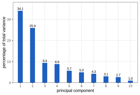
fig_7_22. Reproduces Holmes and Huber (2019), Figure 7.22. Download: PDF · SVGThe correlation circle (Figure 7.23) shows that every event correlates positively with the first component (the loadings range from 0.16 for the 1500 m to 0.43 for the hurdles): PC1 is an overall performance axis, dominated by the sprints, hurdles, long jump and pole vault. The second component opposes the throws (discus 0.81, shot 0.77, javelin 0.59 correlation with PC2) to the 1500 m (\(-0.68\)) and 400 m (\(-0.58\)): strength against endurance. The signs of the axes are arbitrary; here each is fixed so that its largest loading is positive.
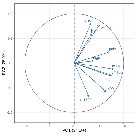
fig_7_23. Reproduces Holmes and Huber (2019), Figure 7.23. Download: PDF · SVG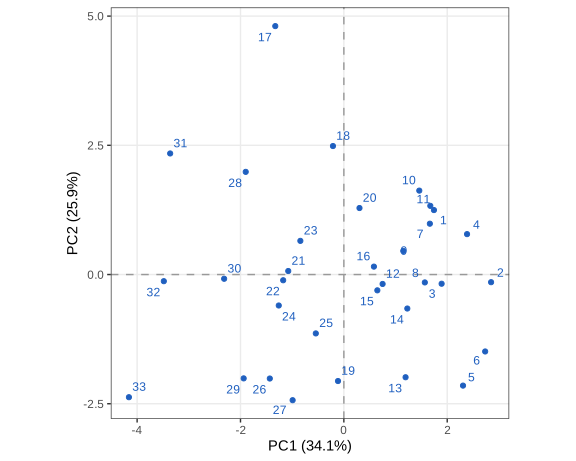
fig_7_24. Reproduces Holmes and Huber (2019), Figure 7.24. Download: PDF · SVGQuestion 7.28 and Figure 7.25. The athletes are listed in the order of their final points, so the drift of low numbers to the right says that PC1 tracks the result. The correlation between PC1 and the points is 0.964. It is not perfect: the points tables score each event by its own nonlinear formula, while PC1 weighs the standardised events linearly by its loadings, giving little weight to the 1500 m and the throws, which load on PC2. Athlete 1 (the gold medallist) has the most points but only the second-highest PC1 score; athlete 2 has the highest.
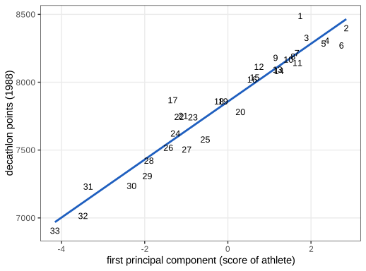
fig_7_25. Reproduces Holmes and Huber (2019), Figure 7.25. Download: PDF · SVG7.7.3 How to choose \(k\), the number of dimensions?
Look at the scree plot first. A clear gap after \(\lambda_k\) suggests keeping \(k\) components. A plateau of similar eigenvalues is a warning: in Figure 7.26 the second, third and fourth eigenvalues are 1.04, 0.95 and 0.90 (14.9%, 13.5%, 12.9% of the variance). A hard rule such as "keep 80% of the variance" would cut inside this plateau (three components give 77.1%, four give 89.9%), and the individual components 2, 3 and 4 cannot be interpreted: only the three-dimensional subspace they span is well determined.
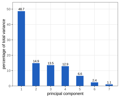
fig_7_26. Reproduces Holmes and Huber (2019), Figure 7.26. Download: PDF · SVGFilling the gap 7.18: why nearly equal eigenvalues give unstable components (a Davis–Kahan bound) Section 7.7.3, Figure 7.26
The book states that "a very slight change in one observation could give a completely different set of three vectors" spanning the same space. Here is the quantitative version: eigenvectors are as stable as the gap that separates their eigenvalue from the others.
Derivation
A 2 × 2 example. Take \(\mathbf{M}=\begin{pmatrix}1+\delta&\varepsilon\\ \varepsilon&1\end{pmatrix}\) with \(\delta\ge0\), a diagonal matrix perturbed by \(\varepsilon\). Its leading eigenvector makes the angle \(\phi\) with the first axis, where \(\tan2\phi=2\varepsilon/\delta\) (the 2 × 2 eigenvector formula, as in Filling the gap 7.5). If \(\delta\gg\varepsilon\), \(\phi\approx\varepsilon/\delta\) is small. If \(\delta=0\), \(\phi=45^\circ\) for every \(\varepsilon\ne0\), however small: with tied eigenvalues an arbitrarily small perturbation decides the direction.
A general bound. Let \(\Sig\) (for instance a population covariance) be symmetric with eigenvalues \(\lambda_1\ge\dots\ge\lambda_p\), let \(\Sh=\Sig+\mathbf{E}\) (for instance a sample covariance, or that of a resampled data set), and let \(\hat{\mathbf{v}}\) be a unit eigenvector of \(\Sh\) with eigenvalue \(\hat\lambda\). Let \(\mathbf{P}\) be the orthogonal projection onto the eigenvectors of \(\Sig\) whose eigenvalues are at distance at least \(\gamma>0\) from \(\hat\lambda\). Then
\[ \|\mathbf{P}\hat{\mathbf{v}}\|\ \le\ \frac{\|\mathbf{E}\|_2}{\gamma}. \]Proof. From \((\Sig+\mathbf{E})\hat{\mathbf{v}}=\hat\lambda\hat{\mathbf{v}}\) we get \((\Sig-\hat\lambda\I)\hat{\mathbf{v}}=-\mathbf{E}\hat{\mathbf{v}}\). \(\mathbf{P}\) commutes with \(\Sig\) (both are diagonal in the eigenbasis of \(\Sig\)), so \((\Sig-\hat\lambda\I)\mathbf{P}\hat{\mathbf{v}}=-\mathbf{P}\mathbf{E}\hat{\mathbf{v}}\). On the range of \(\mathbf{P}\) every eigenvalue of \(\Sig-\hat\lambda\I\) has absolute value at least \(\gamma\), so the left side has norm at least \(\gamma\|\mathbf{P}\hat{\mathbf{v}}\|\), and the right side has norm at most \(\|\mathbf{E}\|_2\). \(\square\)
Now take \(\hat{\mathbf{v}}=\hat{\mathbf{v}}_k\) and let the population gap be \(\delta_k=\min_{j\ne k}|\lambda_j-\lambda_k|\). Weyl's inequality \(|\hat\lambda_k-\lambda_k|\le\|\mathbf{E}\|_2\) (from the min-max characterisation of eigenvalues, since \(|\mathbf{u}^\T\mathbf{E}\mathbf{u}|\le\|\mathbf{E}\|_2\) for unit \(\mathbf{u}\)) puts every other eigenvalue at distance at least \(\gamma=\delta_k-\|\mathbf{E}\|_2\) from \(\hat\lambda_k\). Here \(\mathbf{P}=\I-\mathbf{v}_k\mathbf{v}_k^\T\), so \(\|\mathbf{P}\hat{\mathbf{v}}_k\|=\sin\angle(\hat{\mathbf{v}}_k,\mathbf{v}_k)\), and
\[ \sin\angle(\hat{\mathbf{v}}_k,\mathbf{v}_k)\ \le\ \frac{\|\mathbf{E}\|_2}{\delta_k-\|\mathbf{E}\|_2}\ \le\ \frac{2\|\mathbf{E}\|_2}{\delta_k}\quad\text{when }\|\mathbf{E}\|_2\le\delta_k/2. \]A small gap \(\delta_k\) allows a large rotation.
Groups of eigenvalues. The same argument works for a whole group. Let \(\widehat{\V}_G\in\R^{p\times m}\) hold the estimated eigenvectors of a group, \(\Sh\widehat{\V}_G=\widehat{\V}_G\widehat{\Lam}_G\), and let \(\mathbf{P}\) project onto the population eigenvectors outside the group, whose eigenvalues \(\mu_i\) are at distance at least \(\gamma\) from every \(\hat\lambda\) of the group. Then \(\Sig\mathbf{P}\widehat{\V}_G-\mathbf{P}\widehat{\V}_G\widehat{\Lam}_G=-\mathbf{P}\mathbf{E}\widehat{\V}_G\). In the eigenbasis of \(\Sig\) this reads entrywise \((\mu_i-\hat\lambda_m)Y_{im}=-F_{im}\), so \(|Y_{im}|\le|F_{im}|/\gamma\) and
\[ \|\mathbf{P}\widehat{\V}_G\|_\F\ \le\ \frac{\|\mathbf{E}\widehat{\V}_G\|_\F}{\gamma}\ \le\ \frac{\sqrt m\,\|\mathbf{E}\|_2}{\gamma}. \]The left side is the root sum of squared sines of the principal angles between the estimated and the true group subspaces. Only the gap between the group and the other eigenvalues enters, not the gaps inside the group: tied members may rotate freely among themselves while their span stays put. This is the content of the Davis–Kahan theorem (Davis and Kahan 1970; see Yu, Wang and Samworth 2015 for a version adapted to statistics). Under normality, Anderson (1963) gives the asymptotic covariance of an estimated eigenvector, \(\sum_{j\ne k}\frac{\lambda_k\lambda_j}{n(\lambda_j-\lambda_k)^2}\mathbf{v}_j\mathbf{v}_j^\T\) for distinct eigenvalues, which blows up as two eigenvalues approach each other. ∎
7.8 PCA as an exploratory tool: using extra information
PCA treats all (preprocessed) variables alike, but information that was not used to build the axes helps to interpret them: a diagnosis, a cell type, a final score. Such supplementary information can be projected onto the map without changing it. For the T-cell data of Holmes et al. (2005), the first component carries 63.8% of the variance (Figure 7.27) and orders the cell types naive, memory, effector (mean PC1 scores 11.2, \(-2.3\), \(-10.3\)): memory cells are intermediate (Figure 7.28). The sample labelled MEL53_NAI_3b (naive) sits among the memory cells, the apparently mislabelled sample the book mentions.
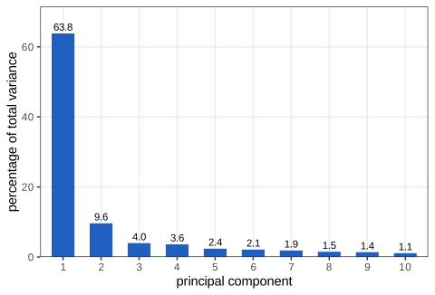
fig_7_27. Reproduces Holmes and Huber (2019), Figure 7.27. Download: PDF · SVG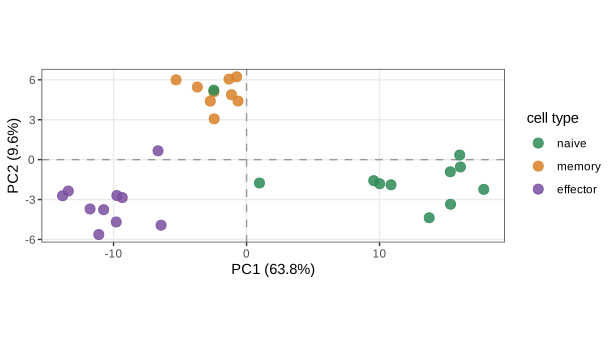
fig_7_28. Reproduces Holmes and Huber (2019), Figure 7.28. Download: PDF · SVGFilling the gap 7.16: supplementary individuals and variables Section 7.8
The book colours points by a factor and plots an external score against PC1. The general device is to project extra rows or columns onto the axes computed from the active data.
Derivation
Supplementary individuals. Let the active data have means \(\bar{\mathbf{x}}\), standard deviations \(s_j\) and loadings \(\V\). A new observation \(\mathbf{x}^\ast\) is preprocessed with the active means and standard deviations, \(\mathbf{z}^\ast=\D^{-1/2}(\mathbf{x}^\ast-\bar{\mathbf{x}})\), and placed at \(\mathbf{c}^\ast=\V^\T\mathbf{z}^\ast\). For an active row this reproduces its score, since the score of row \(i\) is the \(i\)th row of \(\X\V\), i.e. \(\V^\T\mathbf{z}_i\). The new point does not change \(\V\).
Group means. The map \(\mathbf{x}\mapsto\V^\T\D^{-1/2}(\mathbf{x}-\bar{\mathbf{x}})\) is affine, so the projection of a group's mean vector equals the mean of the group's scores: \(\V^\T\D^{-1/2}(\bar{\mathbf{x}}_g-\bar{\mathbf{x}})=\frac{1}{n_g}\sum_{i\in g}\mathbf{c}_i\). A categorical supplementary variable is therefore shown by its groups' barycentres (the large rings of the PCA explorer).
Supplementary variables. A numeric variable \(\mathbf{y}\) not used in the PCA is placed in the correlation circle at \((\cor(\mathbf{y},\mathbf{c}_a),\cor(\mathbf{y},\mathbf{c}_b))\), exactly like an active variable (Filling the gap 7.13). The decathlon points correlate 0.964 with PC1. If \(\mathbf{y}\) were a linear combination of the active variables, its arrow would be inside the circle with squared length equal to the \(R^2\) of its regression on the two components. ∎
7.8.1 Mass spectroscopy data analysis
The matrix mat1 holds 399 aligned mass-spectrometry features for 12 mouse samples, six knockouts and six wild types, with matching numbers (prepared with the Bioconductor package xcms). The first two components explain 43.7% and 15.4% of the variance, 59.1% together (Figures 7.29 and 7.30).
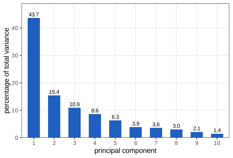
fig_7_29. Reproduces Holmes and Huber (2019), Figure 7.29. Download: PDF · SVG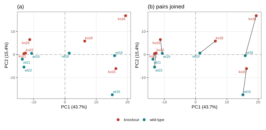
fig_7_30. Reproduces Holmes and Huber (2019), Figure 7.30. Download: PDF · SVGQuestion 7.29. The samples are not placed at random: pairs with the same number sit close together along PC1 (a pair effect, perhaps the day of processing), and within every pair the knockout is shifted in the same direction along PC2. The genotype effect is visible only after the pairing is taken into account, a point the book takes up with supervised methods in the next chapter.
7.8.2 Biplots and scaling
The wine data (178 wines of three cultivars, 13 chemical measurements) are small enough to show samples and variables together. The heat map of \(1-\) correlation (Figure 7.31) groups the phenols, flavonoids and proanthocyanins; Figure 7.32 is the PCA biplot.
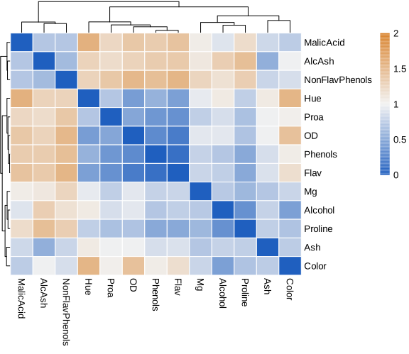
fig_7_31. Reproduces Holmes and Huber (2019), Figure 7.31. Download: PDF · SVG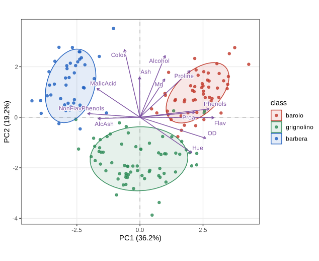
fig_7_32. Reproduces Holmes and Huber (2019), Figure 7.32. Download: PDF · SVGNote on the caption of Figure 7.32
The book's caption says that the axis lengths of each ellipse are one standard deviation. The ellipses are drawn with ellipse.level = 0.69, i.e. as normal-theory 69% regions; for a bivariate normal the region containing probability \(q\) has semi-axes \(\sqrt{\chi^2_{2,q}}\) standard deviations, and with the small-sample correction of stat_ellipse (\(\sqrt{2F_{2,n-1;q}}\)) this is 1.55 for \(n=59\). A one-standard-deviation ellipse contains only \(1-e^{-1/2}=39.3\%\) of a bivariate normal distribution (checked numerically).
Filling the gap 7.14: what a biplot is, and how to read it (Gabriel 1971) Section 7.8.2
The book describes a biplot as observations and variables shown together, with arrows giving the directions of the old variables. The precise statement is a factorisation of the rank-two approximation.
Derivation
Let \(\X_2=\U_2\Sm_2\V_2^\T\) be the rank-two truncation of the preprocessed data. For any \(\alpha\in[0,1]\) put
\[ \mathbf{G}=\U_2\Sm_2^{\alpha}\ (n\times2,\ \text{one point per observation}),\qquad \mathbf{H}=\V_2\Sm_2^{1-\alpha}\ (p\times2,\ \text{one arrow per variable}), \]so that \(\mathbf{G}\mathbf{H}^\T=\X_2\). Every choice gives the inner-product property \(\hat x_{ij}=\mathbf{g}_i^\T\mathbf{h}_j=\|\mathbf{g}_i\|\|\mathbf{h}_j\|\cos\angle(\mathbf{g}_i,\mathbf{h}_j)\): project the points orthogonally onto the line of arrow \(j\), and their order along it is the order of their approximated values of variable \(j\); points beyond the origin on the arrow's side are above average for that variable.
\(\alpha=1\) (the scores \(\U_2\Sm_2=\X\V_2\)): distances between points are exact for the projected rows, \(\|\mathbf{g}_i-\mathbf{g}_l\|=\|\hat{\mathbf{x}}_i-\hat{\mathbf{x}}_l\|\), since \(\V_2\) has orthonormal columns; this is the right choice for reading distances between observations. \(\alpha=0\): \(\mathbf{H}=\V_2\Sm_2\), so \(\mathbf{h}_j^\T\mathbf{h}_l=(\V_2\Sm_2^2\V_2^\T)_{jl}=(\X_2^\T\X_2)_{jl}\approx(n-1)\,\widehat{\cov}(\mathbf{x}_{\cdot j},\mathbf{x}_{\cdot l})\): arrow lengths approximate standard deviations and cosines of angles approximate correlations; for standardised data \(\mathbf{H}/\sqrt{n-1}\) is the correlation circle of Filling the gap 7.13.
The common software display (and Figures 7.19 and 7.32) draws the scores (\(\alpha=1\)) together with correlation arrows (\(\alpha=0\), divided by \(\sqrt{n-1}\)) multiplied by an arbitrary constant to fit the cloud. Each part keeps its own geometry and the projection rule still holds up to that constant factor. Two cautions: angles between arrows are only trustworthy for long arrows, and distances between points are only meaningful when both axes have the same scale (equal aspect ratio; Exercise 7.3). ∎
7.8.3 An example of weighted PCA
The Hiiragi mouse-embryo data (Chapter 3 of the book) have 66 wild-type cells in five groups of very different sizes (36, 11, 11, 4, 4 cells). An ordinary PCA of the 100 most variable genes is dominated by the 36 cells of stage E3.25. Weighting every cell by the inverse of its group size gives each group the same total weight. The weighted first plane explains 26.2% + 14.2% of the weighted variance (Figures 7.33 and 7.34), and the small E4.5 groups now pull the axes as much as the large E3.25 group.
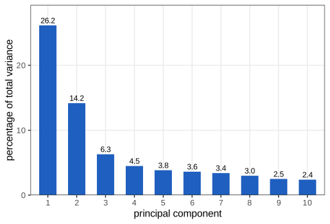
fig_7_33. Reproduces Holmes and Huber (2019), Figure 7.33. Download: PDF · SVG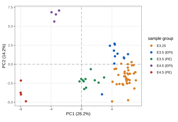
fig_7_34. Reproduces Holmes and Huber (2019), Figure 7.34. Download: PDF · SVGFilling the gap 7.17: PCA with row weights Section 7.8.3
The book passes row.w to dudi.pca. Here is what is being computed, and a scaling detail of ade4.
Derivation
Let \(w_i>0\) with \(\sum_iw_i=1\) and \(\D_w=\diag(w_i)\). The weighted mean is \(\bar{\mathbf{x}}_w=\X^\T\mathbf{w}\), the weighted covariance of the centred matrix \(\X_c=\X-\one\bar{\mathbf{x}}_w^\T\) is \(\Sh_w=\X_c^\T\D_w\X_c\) (and the columns may be standardised with the weighted standard deviations). Weighted PCA maximises the weighted variance \(\mathbf{a}^\T\Sh_w\mathbf{a}\) over unit \(\mathbf{a}\); by Result 7.5 the solution is the eigen-decomposition of \(\Sh_w\), equivalently the SVD \(\D_w^{1/2}\X_c=\U\Sm\V^\T\), with eigenvalues \(s_k^2\) and scores \(\X_c\V\). The scores are uncorrelated in the weighted sense, \(\Cs^\T\D_w\Cs=\Sm^2\). With integer weights this is ordinary PCA of the data in which row \(i\) is repeated in proportion to \(w_i\). With \(w_i\propto1/n_{g(i)}\), group \(g\) has total weight \(n_g\cdot\frac{1}{Gn_g}=\frac1G\): every group contributes equally to the inertia.
The ade4 detail. dudi.pca normalises the weights when it centres and scales, but passes row.w unnormalised to the decomposition. With \(w_i=1/n_g\) the weights sum to \(G=5\), so the reported eigenvalues are five times the weighted variances (they sum to \(5\times100=500\)); percentages and scores are unaffected (checked numerically). ∎
Summary
- Preprocess consciously. Centre always; scale when units differ (correlation PCA is unit-free, covariance PCA is not, Filling the gap 7.15).
- Projection is the basic operation. Regression projects \(\mathbf{y}\) onto the span of the predictors; PCA projects the observations onto the subspace of largest variance, which is also the subspace of smallest perpendicular distance (Filling the gaps 7.5, 7.6).
- The SVD is the computation. \(\X=\U\Sm\V^\T\) always exists (Theorem 7.3); its truncation is the best rank-\(k\) approximation (Theorem 7.4); loadings are \(\V\), scores \(\U\Sm\), variances \(s_k^2/(n-1)\), and the proportion of variance explained equals one minus the relative reconstruction error (Theorem 7.6, Filling the gap 7.12).
- Read the maps with their geometry. Equal scales for the principal plane; correlation circle arrows are correlations, long arrows are well represented, and cosines of angles between long arrows approximate correlations (Filling the gaps 7.13, 7.14).
- Use extra information as supplementary points and variables, and weights when groups are unbalanced (Filling the gaps 7.16, 7.17).
- Check the scree plot before interpreting components: nearly equal eigenvalues give unstable individual components, though the subspace they span is stable (Filling the gap 7.18).
Further reading suggested by the book: Strang (2009) for the linear algebra, Mardia, Kent and Bibby (1979) for classical multivariate analysis with inference on the number of components, Jolliffe (2002) for everything about PCA, Holmes (2006) for weighted ("French school") multivariate analysis, and Zou, Hastie and Tibshirani (2006) and Witten, Tibshirani and Hastie (2009) for sparse PCA.
Exercises
The four exercises of Chapter 7 (Holmes and Huber 2019, Section 7.11), restated in my own words, with worked solutions (hidden). Numbers come from ch07_multivariate_analysis.R; simulated numbers depend on the seed and differ from the book's.
Exercise 7.1 (rank-one and rank-two matrices). (a) A rank-one \(n\times p\) matrix with no zero row or column can be written as a column times a row, \(\X=\mathbf{u}\mathbf{v}^\T\). Is this decomposition unique? (b) Build the outer product of \(\mathbf{u}=(2,4,\dots,30)\) (length 15) and \(\mathbf{v}=(3,6,9,12)\) with
u %*% t(v); why is the transpose needed? (c) Add independent \(\N(1,1)\) noise to get an "approximately rank-one" matrix and visualise it. (d) Repeat with a rank-two matrix.Solution
(a) No. For any \(c\ne0\), \((c\mathbf{u})(\mathbf{v}/c)^\T=\mathbf{u}\mathbf{v}^\T\), so there is a one-parameter family of factorisations, and by Result 7.1 there are no others: any two factorisations have proportional \(\mathbf{u}\)'s (same column space) and proportional \(\mathbf{v}\)'s. Fixing \(\|\mathbf{u}\|=\|\mathbf{v}\|=1\) and pulling out \(s=\|\X\|_\F\) leaves only the joint sign \((\mathbf{u},\mathbf{v})\to(-\mathbf{u},-\mathbf{v})\). The condition "no zero rows or columns" only ensures that all entries of \(\mathbf{u}\) and \(\mathbf{v}\) are nonzero; it does not remove the scaling freedom.
(b) In
%*%a plain vector on the left is treated as a column (15 × 1);t(v)turns \(\mathbf{v}\) into a 1 × 4 row, and the product is the 15 × 4 matrix \(u_iv_j\). Without the transpose R would try an inner product, which fails because the lengths differ (15 and 4).outer(u, v)gives the same matrix.(c) With our seed the singular values of \(\X_1+\text{noise}\) are \(1163.6,\ 4.91,\ 3.43,\ 2.70\): the first piece carries 99.996% of the sum of squares. Two things are going on. The noise has mean 1, so it adds the rank-one matrix \(\one\one^\T\), which is nearly aligned with \(\mathbf{u}\mathbf{v}^\T\) (both have positive entries); and the centred noise is a 15 × 4 matrix of independent \(\N(0,1)\) entries, whose singular values are of order \(\sqrt{15}\pm\sqrt4\), i.e. 2 to 6, tiny next to \(s_1\). A plot of the four columns (say column 1 against column 2, colour by column 3, size by column 4) shows the points on a line with colour and size increasing along it: every column is nearly a multiple of the same \(\mathbf{u}\).
(d) A rank-two matrix is a sum of two outer products, e.g. \(\mathbf{a}_1\mathbf{b}_1^\T+\mathbf{a}_2\mathbf{b}_2^\T\) with random Gaussian vectors. Its rows lie in a plane of \(\R^4\), so it has two nonzero singular values; ours (30 rows, small noise of standard deviation 0.05 added) are \(18.12,\ 6.27,\ 0.32,\ 0.22\), two large and two at the noise level. In the four-variable scatterplot the plane is hard to see by eye, which is the book's point: the SVD finds the dimension that the plot hides.
▶ DemoThe noisy rank-one matrixCompare one piece with the data and look at the residual on its own scale; switch to "noisy rank two" for part (d).Exercise 7.2 (correlated bivariate data). Simulate 50 points from a bivariate normal distribution with standard deviations 2.5 and 0.8 and correlation 0.9 (for instance with
MASS::mvrnorm). Check the rank of the data matrix through its singular values, carry out a PCA and show the data in the rotated principal axes.Solution
Our sample has correlation \(r=0.912\). The singular values of the standardised matrix are \(9.679\) and \(2.077\): both are clearly nonzero, so the matrix has rank two (no 50 × 2 matrix of continuous random data has rank one with positive probability), but the second is small. In fact Filling the gap 7.5 predicts them exactly: for two standardised variables \(s_{1,2}^2=(n-1)(1\pm r)\), so \(s_1=\sqrt{49\times1.912}=9.679\) and \(s_2=\sqrt{49\times0.088}=2.077\), and the first right singular vector is \(\pm(0.707,0.707)\) whatever the data, a consequence of standardising two variables rather than a finding. The rotation itself is
princomp(sim2d)on the unscaled data (the book's text saysprcomp, its code usesprincomp; both give the same rotation, with variances differing by the factor \(n/(n-1)\)). Its scores are the coordinates in the principal axes (Figure 7.35b): the cloud becomes an ellipse aligned with the axes, uncorrelated, with standard deviations \(\sqrt{\lambda_1}\) and \(\sqrt{\lambda_2}\).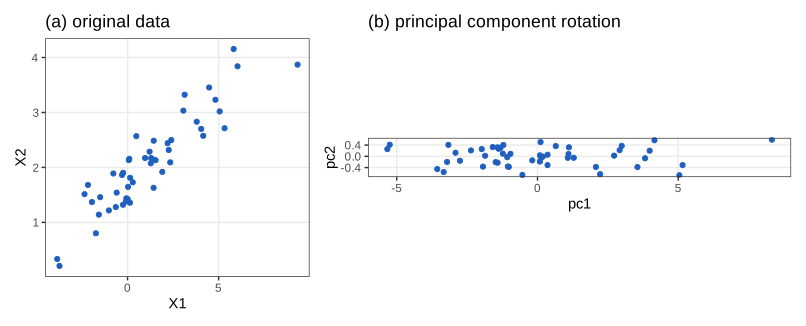
Figure 7.35. (a) The simulated data drawn without equal scales; (b) the same data in principal component coordinates, drawn with equal scales, so the band is long and thin. The book draws (b) with coord_fixed(2), which doubles the vertical scale; here the ratio is 1. Code: ch07_multivariate_analysis.R,fig_7_35. Reproduces Holmes and Huber (2019), Figure 7.35. Download: PDF · SVGExercise 7.3 (aspect ratio). Why is the plotting region of Figure 7.35(a) elongated? What happens with a square plotting region and no
coord_fixed(), and why can that mislead?Solution
With equal scales (one unit is the same length on both axes) the shape of the plotting region follows the ranges of the data: the first variable has standard deviation about 2.65 and the second about 0.84 in our sample, so an equal-scaled plot is about three times wider than high. Without
coord_fixed()ggplot stretches each axis to fill the panel, here a square: the short direction is magnified about three times. This (i) makes the cloud look rounder and the variance along the minor axis look comparable to the major one, the opposite of what the singular values say; (ii) destroys right angles, so perpendicular projections no longer look perpendicular and the principal axis is no longer drawn at its true angle; (iii) makes Euclidean distances between points unreadable, because a horizontal and a vertical step of the same length on the page correspond to different distances in the data. For PCA maps, whose whole point is distances and directions, equal scales are essential (the book's remark under Figure 7.19). The same objection applies to the book'scoord_fixed(2)in Figure 7.35(b), which doubles the vertical scale.Exercise 7.4 (weighted versus unweighted PCA of the Hiiragi data). (a) Draw the correlation circle of the unweighted PCA of the 66 wild-type cells and the 100 most variable genes. Which genes are best represented in the first principal plane? (b) Make a biplot showing the labels of the genes that explain most of the variance in this plane, together with the cells.
Solution
(a) The unweighted first plane explains 21.9% + 8.1% of the variance (against 26.2% + 14.2% for the weighted analysis of Section 7.8.3, where the small E4.5 groups have more influence). "Best represented" means largest squared arrow length \(\cor(\mathbf{x}_j,\mathbf{c}_1)^2+\cor(\mathbf{x}_j,\mathbf{c}_2)^2\), the fraction of the gene's variance captured by the plane (Filling the gap 7.13). The top genes are Pramel6 (0.843), Bhmt (0.838), Spic (0.812), Lama1 (0.784) and Fgf4 (0.782 and 0.781 for two probes); Pramel6, Bhmt and Spic lie along PC1 on the positive side, Lama1 and Serpinh1 (0.731) on the negative side, and the two Fgf4 probes along PC2.
(b) Compute the PCA (for example
pca_svdin the course code, ordudi.pca), order the genes by the squared length above, and draw the scores of the cells (coloured by group) with arrows and labels for, say, the 10 best represented genes, stretched by a common factor (Filling the gap 7.14). Cells lying in the direction of a gene's arrow have high expression of that gene. The PCA explorer does this interactively: choose "mouse embryo genes", tick the biplot arrows (it labels the 12 longest arrows in the chosen plane) and compare the row weights "equal" and "1 / group size".▶ DemoMouse embryo genes in the PCA explorerStart from the weighted analysis and switch to equal weights for part (a).
Demonstrations for this chapter
Each demonstration runs in the browser on the chapter's data (exported by the R code), uses seeded random numbers where there is randomness, and links back to these notes. The ▶ Demo boxes above open them at the case under discussion. Their numbers agree with R: for example the variance along the first principal line of discus and weight is 1.806352 in both, the singular values of Xtwo agree to \(10^{-12}\), and the explorer's eigenvalues match dudi.pca to six or more significant digits.
| Demonstration | What you can see | Sections |
|---|---|---|
| Regression lines and the principal component line | Any two decathlon events, standardised or in their own units: the two regression lines, the principal component line, and a line you rotate, with the variance along it and the mean squared distance to it. Presets: 1 the three lines (Fig. 7.11); 2 rotate the line (Q. 7.8); 3 vertical residuals (Fig. 7.8, Q. 7.6); 4 original units (Q. 7.7); 5 weak correlation. | 7.3.1, 7.3.2, 7.4.1 (gaps 7.3–7.6) |
| The SVD and the best rank-k approximation | Heat maps of a matrix, its rank-k truncation and the residual; the squared singular values; the error against k; random rank-k competitors that never win. Presets: 1 rank one (Figs 7.15, 7.16); 2 Xtwo (Q. 7.16); 3 noisy rank one (Ex. 7.1); 4 turtles; 5 Eckart–Young on the decathlon. | 7.6.1–7.6.3 (Thm 7.3, Thm 7.4) |
| PCA explorer: scree plot, principal plane, correlation circle and biplot | Seven data sets of the chapter; correlation or covariance PCA; equal or inverse-group-size weights; any pair of the first three axes; arrows, group means and a supplementary variable. Presets: 1 turtles (Figs 7.18–7.20); 2 decathlon with the points (Figs 7.22–7.25); 3 scaling matters; 4 wine biplot (Fig. 7.32); 5 weighted mouse embryos (Figs 7.33, 7.34). | 7.5, 7.7, 7.8 (Thm 7.6, gaps 7.11–7.17) |
| When are principal components stable? | Bootstrap resamples of the data: eigenvalues, angles of the resampled components to the originals, the largest principal angle of a group's subspace, and the loadings of a chosen component. Presets: 1 the data of Fig. 7.26; 2 its stable first component; 3 the decathlon; 4 simulated, large gap; 5 simulated, no gap. | 7.7.3 (gap 7.18) |
The R code that produces every figure of this page is code/ch07_multivariate_analysis.R (see the code index). Figures not reproduced: 7.1 and 7.21 (cartoons), 7.12 and 7.14 (photographs of shadows of an object), 7.13 (a hand-drawn workflow diagram).
References
- Holmes, S. and Huber, W. (2019). Modern Statistics for Modern Biology. Cambridge University Press, Cambridge. Chapter 7.
- Anderson, T. W. (1963). Asymptotic theory for principal component analysis. The Annals of Mathematical Statistics, 34(1), 122–148.
- Davis, C. and Kahan, W. M. (1970). The rotation of eigenvectors by a perturbation. III. SIAM Journal on Numerical Analysis, 7(1), 1–46. doi:10.1137/0707001.
- Eckart, C. and Young, G. (1936). The approximation of one matrix by another of lower rank. Psychometrika, 1(3), 211–218. doi:10.1007/BF02288367.
- Fan, K. (1949). On a theorem of Weyl concerning eigenvalues of linear transformations I. Proceedings of the National Academy of Sciences, 35(11), 652–655. doi:10.1073/pnas.35.11.652. (The maximum principle in step 3 of Filling the gap 7.9.)
- Gabriel, K. R. (1971). The biplot graphic display of matrices with application to principal component analysis. Biometrika, 58(3), 453–467. doi:10.1093/biomet/58.3.453.
- Holmes, S. (2006). Multivariate data analysis: the French way. In D. Nolan and T. Speed (eds), Probability and Statistics: Essays in Honor of David A. Freedman, IMS Lecture Notes–Monograph Series 56.
- Holmes, S., He, M., Xu, T. and Lee, P. P. (2005). Memory T cells have gene expression patterns intermediate between naive and effector. Proceedings of the National Academy of Sciences, 102(15), 5519–5523.
- Hotelling, H. (1933). Analysis of a complex of statistical variables into principal components. Journal of Educational Psychology, 24(6), 417–441. doi:10.1037/h0071325.
- Jolicoeur, P. and Mosimann, J. E. (1960). Size and shape variation in the painted turtle. A principal component analysis. Growth, 24, 339–354.
- Jolliffe, I. T. (2002). Principal Component Analysis, 2nd edition. Springer, New York.
- Kaiser, H. F. (1960). The application of electronic computers to factor analysis. Educational and Psychological Measurement, 20(1), 141–151.
- Mardia, K. V., Kent, J. T. and Bibby, J. M. (1979). Multivariate Analysis. Academic Press, London.
- Mirsky, L. (1960). Symmetric gauge functions and unitarily invariant norms. The Quarterly Journal of Mathematics, 11(1), 50–59. doi:10.1093/qmath/11.1.50.
- Pearson, K. (1901). On lines and planes of closest fit to systems of points in space. The London, Edinburgh, and Dublin Philosophical Magazine and Journal of Science, 2(11), 559–572. doi:10.1080/14786440109462720.
- Strang, G. (2009). Introduction to Linear Algebra, 4th edition. Wellesley-Cambridge Press.
- Witten, D. M., Tibshirani, R. and Hastie, T. (2009). A penalized matrix decomposition, with applications to sparse principal components and canonical correlation analysis. Biostatistics, 10(3), 515–534. doi:10.1093/biostatistics/kxp008.
- Yu, Y., Wang, T. and Samworth, R. J. (2015). A useful variant of the Davis–Kahan theorem for statisticians. Biometrika, 102(2), 315–323. doi:10.1093/biomet/asv008.
- Zou, H., Hastie, T. and Tibshirani, R. (2006). Sparse principal component analysis. Journal of Computational and Graphical Statistics, 15(2), 265–286. doi:10.1198/106186006X113430.
Every number quoted in the text (eigenvalues, singular values, correlations, percentages, the counterexample to Question 7.24, the correction to Question 7.27, the ellipse radius of Figure 7.32 and the ade4 weight scaling) is computed by the course R code.