Chapter 5. Clustering
Clustering adds a new categorical variable, the group, to a table of objects described by features. This chapter of Holmes and Huber (2019) starts from the choice of a distance, then studies partitioning methods (k-means, k-medoids and PAM), density-based clustering of cytometry data, hierarchical clustering, the validation of a clustering and the choice of the number of clusters (the within-cluster sum of squares, the Calinski-Harabasz index, the gap statistic, silhouettes, resampling), and finally clustering as a way to remove noise from sequencing reads. The book is applied and states most results without proof; these notes supply the arguments: why each distance is a metric, why k-means and PAM stop, what DBSCAN's clusters are, why dendrograms are ultrametrics, where the gap statistic's standard error comes from, and how unequal group sizes move a decision boundary.
Ch. 1 Discrete data Ch. 2 Statistical modeling Ch. 3 Data visualization Ch. 4 Mixture models Ch. 5 Clustering Ch. 6 Testing Ch. 7 Multivariate analysis Ch. 8 Count data and GLMs Ch. 9 Heterogeneous data Ch. 10 Networks and trees Ch. 11 Image data Ch. 12 Supervised learning Ch. 13 Experimental design
How to read these notes
They follow the book. Sections carry the book's numbers (5.3, 5.7.1, ...), and equations quoted from the book carry its numbers, e.g. (5.7). Figures carry the book's figure numbers. Questions asked in the text of the book are restated where they appear (as "Question 5.k"), and the end-of-chapter exercises are in the Exercises section.
Filling the gaps. Wherever the book states a result without derivation, an orange Filling the gap box gives the full argument, with its assumptions. Proofs start hidden: open one with its bar, or use the button below. Places where the printed text is wrong are marked Erratum, with the evidence.
Figures, code and demonstrations. Every figure computed from data or by simulation is reproduced by code/ch05_clustering.R; photographs, maps and schematics are not. The ▶ Demo boxes open an interactive page already set to the case under discussion.
Main reference
S. Holmes and W. Huber, Modern Statistics for Modern Biology, Cambridge University Press (2019), Chapter 5 (Clustering). Section, equation, figure, question and exercise numbers below refer to this book. Further reading is listed in the references.
The explanations, derivations and code are my own; results are cited by their numbers in the book.
The chapter at a glance
- 5.3 A clustering is only as good as its notion of distance. Minkowski distances with \(m\ge1\) are metrics, with \(m<1\) they are not; the Mahalanobis distance is the Euclidean distance after whitening; the Jaccard and edit distances are metrics; the correlation distance is a Euclidean distance between standardised profiles.
- 5.4 k-means is coordinate descent on \(J=\sum_i|x_i-c_{\ell(i)}|^2\) and stops after finitely many steps at a local minimum. k-medoids and PAM replace means by data points and allow any dissimilarity.
- 5.5 The asinh transform makes cytometry intensities nearly homoscedastic (it is the variance-stabilising transformation for variance \(a+b\mu^2\)). DBSCAN's clusters are the connected components of the graph of core points, with border points attached.
- 5.6 Hierarchical clustering merges the two closest clusters; the linkages obey the Lance-Williams recursion, monotone linkages give ultrametric trees, single linkage is the minimum spanning tree, Ward merges by the smallest increase of the within sum of squares.
- 5.7 \(\WSS_k\) equals a sum of squared pairwise distances, \(\TSS=\WSS+\BSS\), the Calinski-Harabasz index is an \(F\) ratio, and the gap statistic calibrates \(\log W_k\) against uniform reference data with a one-standard-error rule.
- 5.8 With unequal abundances the Bayes boundary moves towards the rare group by \(\sigma^2\log(\pi_2/\pi_1)/|\mu_2\)
\({}-\mu_1|\); error counts per read are binomial, close to Poisson; DADA2 uses abundance p-values.
Notation. Observations \(x_1,\dots,x_n\in\R^p\) (rows of the data table), a dissimilarity \(d(x_i,x_j)=d_{ij}\), a partition of \(\{1,\dots,n\}\) into clusters \(C_1,\dots,C_k\) with sizes \(n_\ell=|C_\ell|\), cluster means \(\bar x_\ell\), overall mean \(\bar x\), and \(|v|\) the Euclidean norm of a vector \(v\).
Prerequisites. Mixture models and the EM algorithm (Chapter 4), the bootstrap (Chapter 4), the delta method and variance-stabilising transformations (Chapters 4 and 8), the multivariate normal distribution.
5.2 What are the data and why do we cluster them?
5.2.1 Clustering can lead to discoveries
Section 5.2.1, Figures 5.1–5.4 Three historical examples open the chapter. John Snow's map of cholera deaths (Figure 5.1 of the book, a historical map) showed a spatial cluster of cases around one water pump, which pointed to the water as the cause. The map of bomb impacts on London in 1940 (Figure 5.2, a map) shows the opposite lesson: apparent clusters that analysts tried to explain turned out to be random. Molecular clustering of breast tumours (Figure 5.3, a published figure of Aure et al. 2017) found subgroups with different survival, which is the kind of discovery that motivates clustering in biology.
The methods of Chapter 4 modelled each group by a parametric density. The methods here are mostly based on distances between pairs of observations and assume no family of distributions. Figure 5.4 of the book (a schematic) lays out the choices: a table \(X\) (observations by features), a distance, the matrix of all pairwise distances, and then either an agglomerative (hierarchical) method, which postpones the choice of the number of clusters \(k\), or a partitioning method, which needs \(k\) at the outset.
The caveat of the chapter deserves to be stated first: a clustering algorithm always returns clusters, whether the data have any or not. Section 5.7 is about deciding whether they are real.
5.3 How do we measure similarity?
Section 5.3, (5.1)–(5.6), Figures 5.5–5.9 Question 5.1 of the book shows pictures of two cats and two dogs and asks which are most alike. The answer depends on what you care about (species, or behaviour, or appearance): similarity is a choice. Before any formula one must decide which features to include, on what scale, and after which transformation (for instance standardising each feature by its standard deviation, which weights all features equally).
Definition 5.1 (dissimilarity, metric, ultrametric) Section 5.3
A dissimilarity on a set \(\mathcal{X}\) is a function \(d:\mathcal{X}\times\mathcal{X}\to[0,\infty)\) with \(d(x,x)=0\) and \(d(x,y)=d(y,x)\). It is a metric if in addition
- \(d(x,y)=0\) only if \(x=y\) (identity of indiscernibles), and
- \(d(x,z)\le d(x,y)+d(y,z)\) for all \(x,y,z\) (triangle inequality).
A metric is an ultrametric if it satisfies the stronger inequality \(d(x,z)\le\max\{d(x,y),d(y,z)\}\). A dissimilarity that satisfies everything except (1) is a pseudometric: it is a metric on the classes of points at distance 0. The book's remark that "any metric space will do" means that clustering needs only the numbers \(d_{ij}\), not coordinates.
The book lists the distances most used in biology.
- Euclidean (5.1): \(d(A,B)=\sqrt{\sum_{j=1}^p(a_j-b_j)^2}\). Its equal-distance contours are circles (Figure 5.5).
- Weighted Euclidean: \(\sqrt{\sum_j w_j(a_j-b_j)^2}\) with \(w_j>0\); the \(\chi^2\) distance of Chapter 2 is the case \(w_j=1/(\text{expected count})\). The Mahalanobis distance \(\sqrt{(a-b)^\T S^{-1}(a-b)}\) with a covariance matrix \(S\) also accounts for correlations; its contours are ellipses (Figure 5.6).
- Minkowski (5.2): \(d(A,B)=\big(\sum_j|a_j\)
\({}-b_j|^m\big)^{1/m}\); \(m=1\) is the Manhattan distance (5.3) with diamond-shaped contours (Figure 5.7), and \(m\to\infty\) the maximum distance (5.4), \(\max_j|a_j-b_j|\), with square contours (Figure 5.8). - Edit (Levenshtein) and Hamming distances between strings: the Hamming distance counts differing positions of two strings of equal length; the edit distance is the smallest number of substitutions, insertions and deletions turning one string into the other.
- Binary and Jaccard: for presence/absence vectors, with \(f_{11}\) the number of features present in both, \(f_{10},f_{01}\) present in only one and \(f_{00}\) in neither, the Jaccard index is \(J=f_{11}/(f_{01}+f_{10}+f_{11})\) (5.5) and the Jaccard distance \(1-J\) (5.6). Co-absences are ignored. R's
dist(method = "binary")is exactly this distance. - Correlation-based: \(d(A,B)=\sqrt{2(1-\operatorname{cor}(A,B))}\), which is 0 for perfectly correlated profiles, \(\sqrt2\) for uncorrelated and 2 for perfectly anticorrelated ones.
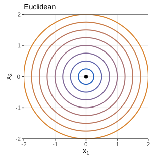
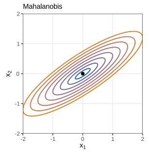
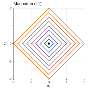
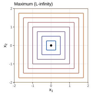
Figures 5.5–5.8 are drawn in the book as sketches; here each is computed: contours at distances 0.25, 0.5, ..., 2 from the origin. Code: fig_5_5 to fig_5_8.
Filling the gap 5.1: which Minkowski distances are metrics Section 5.3, (5.1)–(5.4)
The book introduces (5.2) with any exponent \(m\). Write \(\|v\|_m=(\sum_j|v_j|^m)^{1/m}\), so \(d_m(A,B)=\|A-B\|_m\).
Claim. (a) For \(m\ge1\), \(d_m\) is a metric. (b) For \(0<m<1\) it is not. (c) \(\lim_{m\to\infty}d_m(A,B)\)
Proof
Symmetry, \(d_m\ge0\) and \(d_m(A,B)=0\iff A=B\) are immediate. Because \(d_m(A,C)=\|(A-B)+(B-C)\|_m\), the triangle inequality is the statement \(\|u+v\|_m\le\|u\|_m+\|v\|_m\) (Minkowski's inequality).
(a) For \(m=1\) it follows from \(|u_j+v_j|\le|u_j|+|v_j|\) summed over \(j\). For \(m>1\) let \(q=m/(m-1)\), so \(1/m+1/q=1\). Hölder's inequality states \(\sum_j|a_jb_j|\le\|a\|_m\|b\|_q\); it follows from Young's inequality \(st\le s^m/m+t^q/q\) (\(s,t\ge0\), a consequence of the concavity of the logarithm) applied to \(s=|a_j|/\|a\|_m\), \(t=|b_j|/\|b\|_q\) and summed. Now write
\[ \|u+v\|_m^m=\sum_j|u_j+v_j|\,|u_j+v_j|^{m-1}\le\sum_j|u_j|\,|u_j+v_j|^{m-1}+\sum_j|v_j|\,|u_j+v_j|^{m-1}. \]Apply Hölder to each sum with \(b_j=|u_j+v_j|^{m-1}\), for which \(\|b\|_q=(\sum_j|u_j+v_j|^{(m-1)q})^{1/q}\)
(b) Take \(A=(0,0)\), \(C=(1,0)\), \(B=(1,1)\) in the plane. Then \(d_m(A,C)=d_m(C,B)=1\) while \(d_m(A,B)=2^{1/m}>2\) when \(m<1\): the triangle inequality fails (for \(m=1/2\), \(4>2\)). Geometrically, the unit "ball" \(\{v:\|v\|_m\le1\}\) is not convex for \(m<1\), and a norm's unit ball is always convex.
(c) Let \(M=\max_j|v_j|\). Then \(M^m\le\sum_j|v_j|^m\le pM^m\), so \(M\le\|v\|_m\le p^{1/m}M\), and \(p^{1/m}\to1\). The triangle inequality for \(d_\infty\) follows from \(|u_j+v_j|\le\max|u|+\max|v|\) for each \(j\). ∎
We verify the triangle inequality for \(m=1,2,3,\infty\) on random triples, the counterexample for \(m=1/2\), and the limit (c).
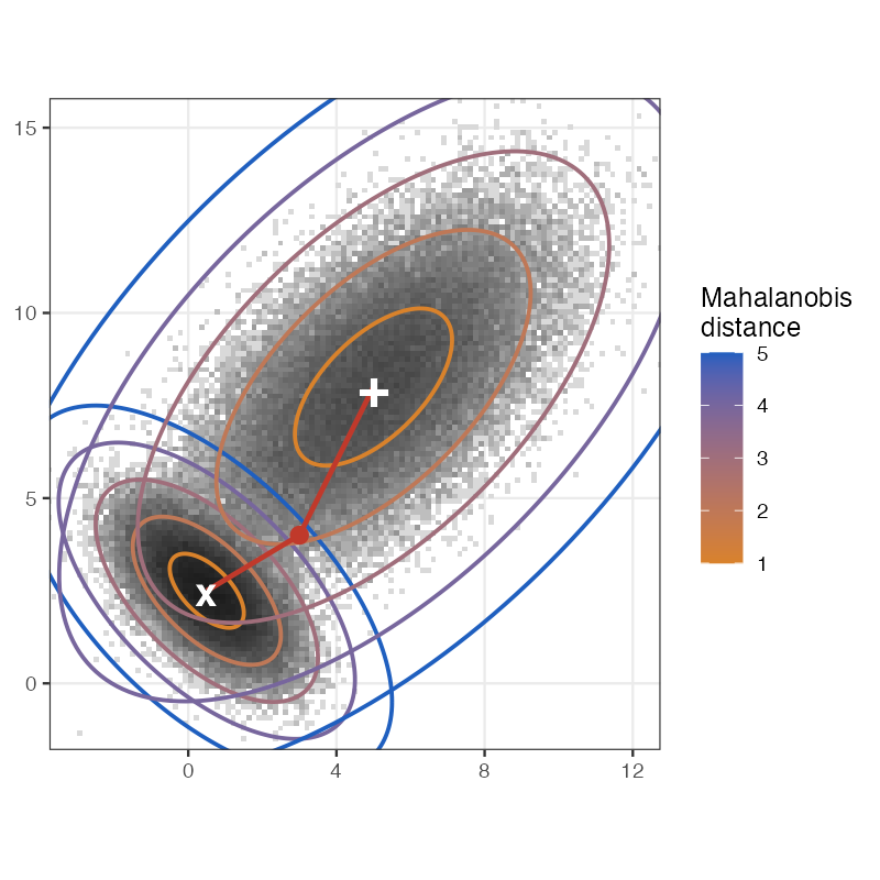
fig_5_9. Reproduces Holmes and Huber (2019), Figure 5.9. PDFQuestion 5.2 (book) asks which centre the red point of Figure 5.9 is closest to. Measured in units of each group's own spread, it is the right-hand group: the point lies on the 1.9 contour of the large group but beyond the 4.5 contour of the small one. The book explains this by counting density contours; the Mahalanobis distance is the version of that count for normal densities, as the next box shows.
Filling the gap 5.2: the Mahalanobis distance Section 5.3, Question 5.2, Figure 5.9
Let \(S\) be a symmetric positive definite \(p\times p\) matrix and \(d_S(x,y)=\sqrt{(x-y)^\T S^{-1}(x-y)}\).
Claim. (a) \(d_S(x,y)=|L^{-1}(x-y)|\) for any \(L\) with \(LL^\T=S\) (for instance the Cholesky factor or the symmetric square root \(S^{1/2}\)); hence \(d_S\) is the Euclidean distance after the linear "whitening" map \(x\mapsto L^{-1}x\), and is a metric. (b) If \(X\sim\N(\mu,S)\) then the density of \(X\) is a decreasing function of \(d_S(X,\mu)\), its contours are the ellipsoids \(d_S(x,\mu)=r\), and \(d_S(X,\mu)^2\sim\chi^2_p\). (c) The Euclidean distance is the case \(S=I\), the weighted Euclidean distance the case \(S\) diagonal.
Proof
(a) \(S^{-1}=(LL^\T)^{-1}=L^{-\T}L^{-1}\), so \((x-y)^\T S^{-1}(x-y)\)
(b) The normal density is \((2\pi)^{-p/2}\det(S)^{-1/2}\exp\{-\tfrac12d_S(x,\mu)^2\}\), a decreasing function of \(d_S(x,\mu)\), so "the number of density contours crossed", as in the book's solution to Question 5.2, is a monotone function of \(d_S\). Put \(Z=L^{-1}(X-\mu)\). Then \(Z\) is normal with mean 0 and covariance \(L^{-1}SL^{-\T}=I\), so its coordinates are independent standard normals and \(d_S(X,\mu)^2=|Z|^2\)
(c) is immediate. ∎
In Figure 5.9 each group has its own \(S\), so the "distance" from a point to group \(g\) is \(d_{S_g}(x,\mu_g)\); as a function of two points with different matrices it is no longer one metric, but it is the natural classification score: up to the constant \(\tfrac12\log\det S_g\) it is \(-2\) times the log-density of group \(g\) (quadratic discriminant analysis, Chapter 12 of the book). The numbers in the caption and the \(\chi^2_2\) law of \(d_S^2\) are verified numerically.
Filling the gap 5.3: the Jaccard and correlation distances are metrics Section 5.3, (5.5), (5.6)
Claim. (a) Identify a presence/absence vector with the set \(A\) of its present features. Then the Jaccard distance \(d_J(A,B)=|A\triangle B|/|A\cup B|\) (with \(d_J(\emptyset,\emptyset)=0\)) is a metric. (b) For profiles \(a,b\in\R^p\) with standardised versions \(z_a=(a-\bar a)/s_a\) (sample standard deviation \(s_a\)), \(\sqrt{2(1-r_{ab})}\)
Proof
(a) Note \(|A\triangle B|=f_{10}+f_{01}\) and \(|A\cup B|=f_{11}+f_{10}+f_{01}\), so this is (5.6). Symmetry and \(d_J(A,B)=0\iff A=B\) are clear. For the triangle inequality the standard trick is to show that \(d_J(A,B)\) is a probability. Let \(\pi\) be a uniformly random ordering of all features and \(h(A)\) the first feature of \(A\) in that ordering (min-hashing). The first element of \(A\cup B\) is equally likely to be any element of \(A\cup B\); it is the first of both \(A\) and \(B\) exactly when it lies in \(A\cap B\). Hence \(\Prob\{h(A)\ne h(B)\}\)
(b) \(|z_a-z_b|^2=|z_a|^2+|z_b|^2\)
We confirm that dist(method = "binary") reproduces the book's values 0.6, 0.667, 0.5 by (5.6), that vegan::vegdist(mut, "jaccard") equals (5.6) on the HIV data, the triangle inequality on random sets, and identity (b) on the HIV data.
Filling the gap 5.4: computing the edit distance, and why it is a metric Section 5.3, "Edit, Hamming"
Let \(s=s_1\cdots s_m\), \(t=t_1\cdots t_n\) and let \(D(i,j)\) be the edit distance between the prefixes \(s_1\cdots s_i\) and \(t_1\cdots t_j\). Then \(D(i,0)=i\), \(D(0,j)=j\) and
\[ D(i,j)=\min\big\{D(i-1,j)+1,\;D(i,j-1)+1,\;D(i-1,j-1)+\ind[s_i\ne t_j]\big\}, \]so the distance \(D(m,n)\) costs \(O(mn)\) operations. It is a metric on strings.
Proof
Take an optimal sequence of edits and align the two prefixes: the last column of the alignment either deletes \(s_i\), inserts \(t_j\), or pairs \(s_i\) with \(t_j\) (free if equal, one substitution if not). Removing that column leaves an alignment of shorter prefixes, which must itself be optimal (otherwise the whole could be improved), giving the three candidates; conversely each candidate is achievable. Metric: \(D=0\) only for equal strings; edits are reversible with equal cost (insertion and deletion swap), giving symmetry; and editing \(s\) into \(u\) and then \(u\) into \(t\) is one way of editing \(s\) into \(t\), so \(D(s,t)\le D(s,u)+D(u,t)\). ∎
Biological versions replace the unit costs by substitution scores and gap penalties (the Needleman-Wunsch recursion has the same form). With positive gap costs and symmetric substitution costs that themselves satisfy the triangle inequality the result is still a metric. We compare this recursion with utils::adist and test the triangle inequality.
5.3.1 Computations related to distances in R
Section 5.3.1, Figures 5.10, 5.11 For \(n\) objects there are \(n(n-1)/2\) distinct distances; dist stores only these (the lower triangle, Figure 5.10 of the book) and offers six methods (euclidean, maximum, manhattan, canberra, binary, minkowski). For the three binary vectors of the book, the Euclidean distances are \(\sqrt3,2,\sqrt3\) and the binary (Jaccard) distances \(0.6,0.667,0.5\); on the Morder T-cell data the distance between samples 1 and 2 is 5.593667, whichever way it is computed. These numbers are reproduced in R.
Question 5.3 (book) compares the Jaccard distance between the 5 HIV strains of HIVmutations.csv (57 mutation indicators) with the correlation distance. The two orderings agree almost perfectly: over the 10 pairs the Spearman correlation between the two distances is 0.991. This is no accident: for 0/1 vectors with a small fraction of ones, \(1-r\) is driven by the same counts \(f_{10}+f_{01}\) relative to \(f_{11}\), because the many co-absences hardly change the correlation. The Jaccard distance is the more interpretable one (it ignores co-absences by design).
Distances exist for many other objects: Gower's distance for mixed data (daisy), shortest-path distances on graphs, the cophenetic distance between leaves of a tree (the height at which they are joined; Figure 5.11 of the book, a cartoon, and Filling the gap 5.10), distances between trees, geodesic distances on a sphere. Choosing a distance that matches the scientific question is the most consequential step of a clustering.
5.4 Nonparametric mixture detection
5.4.1 k-methods: k-means, k-medoids and PAM
Section 5.4.1, Figure 5.12, Question 5.4 Partitioning (iterative relocation) methods need a distance and the number of clusters \(k\). The book describes k-medoids as: pick \(k\) observations at random as centres, assign each observation to the closest centre, replace each centre by the medoid of its group (the member with the smallest sum of distances to the other members), and repeat until the groups no longer change. Replacing the medoid by the arithmetic mean gives k-means, which is tied to the squared Euclidean distance.
Filling the gap 5.5: k-means is coordinate descent and stops after finitely many steps Section 5.4.1, Figure 5.12
For centres \(c_1,\dots,c_k\in\R^p\) and an assignment \(\ell:\{1,\dots,n\}\to\{1,\dots,k\}\) let
\[ J(c,\ell)=\sum_{i=1}^n|x_i-c_{\ell(i)}|^2. \]Lloyd's algorithm alternates (A) \(\ell(i)\leftarrow\argmin_m|x_i-c_m|^2\) and (U) \(c_m\leftarrow\bar x_m\), the mean of the points assigned to \(m\).
Claim. (a) For fixed \(\ell\), \(J(c,\ell)=\WSS(\ell)+\sum_m n_m|\bar x_m\)
Proof
(a) For the points \(i\) with \(\ell(i)=m\), expand \(x_i-c_m=(x_i-\bar x_m)+(\bar x_m-c_m)\):
\[ \sum_{\ell(i)=m}|x_i-c_m|^2=\sum_{\ell(i)=m}|x_i-\bar x_m|^2+n_m|\bar x_m-c_m|^2+2(\bar x_m-c_m)^\T\sum_{\ell(i)=m}(x_i-\bar x_m), \]and the last sum is zero by definition of \(\bar x_m\). Summing over \(m\) gives the identity; the second term is \(\ge0\) and vanishes exactly for \(c_m=\bar x_m\). (An empty cluster contributes nothing and its centre can stay where it is.)
(b) \(J\) is a sum of terms that each depend on one \(\ell(i)\); each is minimised separately by the nearest centre.
(c) Let \(J_t\) be the value after the \(t\)-th half step. By (a) and (b), \(J_{t+1}\le J_t\). Suppose the algorithm visited the same assignment twice with a strict decrease in between: after (U) the value is \(\WSS(\ell)\), a function of the assignment alone, so returning to \(\ell\) gives the same value, a contradiction. Hence, as long as the algorithm continues, the post-update values \(\WSS(\ell_t)\) strictly decrease (ties in (A) broken consistently, e.g. by keeping the current centre), assignments never repeat, and there are at most \(k^n\) of them. When (A) changes nothing the next (U) changes nothing either, so the algorithm has stopped. ∎
Only a local minimum. Minimising \(\WSS\) over all partitions is NP-hard in general, and Lloyd's algorithm can stop at a poor partition: on the four-group simulation of Section 5.7 with \(k=3\), one random start ends at \(J=6050\) while the best value is 5498 (demo, preset 2). This is why kmeans has an nstart argument and why the book stresses that different seeds give different results.
Relation to EM (Question 5.4). Fit a mixture of \(k\) normals with equal weights and common covariance \(\sigma^2I\) by EM. The E step gives responsibilities \(\gamma_{im}\propto\exp(\)
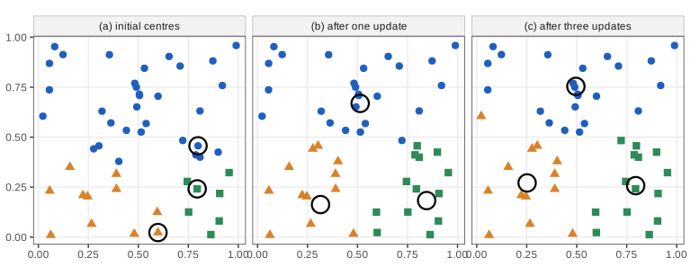
kmeans with its default Hartigan-Wong algorithm). Code: fig_5_12. Reproduces Holmes and Huber (2019), Figure 5.12. PDF · SVGThe k-methods work best for groups of similar size that are convex and roughly spherical. A large group tends to be split, and elongated or non-convex groups are cut across (the spirals of Exercise 5.3): every k-means cluster is a cell \(\{x:|x-c_m|\le|x-c_{m'}|\ \forall m'\}\), an intersection of half-spaces, hence convex.
Filling the gap 5.6: medoids, PAM's BUILD and SWAP, and why they stop Section 5.4.1; Kaufman and Rousseeuw (2009)
For any dissimilarity \(d\) and a set \(M\) of \(k\) data points (medoids), let \(\operatorname{TD}(M)\)
Claim. (a) The alternating algorithm described in the book never increases \(\operatorname{TD}\) and stops after finitely many steps. (b) PAM (Algorithm 5.1, as implemented by cluster::pam) also decreases \(\operatorname{TD}\) strictly at each swap and stops. (c) Its stopping point is "swap-optimal": no exchange of one medoid with one non-medoid helps. Every swap-optimal configuration is also a stopping point of the alternating algorithm, but not conversely, so PAM's stopping points are a smaller, better set. (d) For \(p=1\) and \(d(x,y)=|x-y|\), the best single centre (not restricted to data points) is the median; this is why medoids with the Manhattan distance are robust to outliers.
Proof
(a) Write \(\operatorname{TD}(M,\ell)\)
(b) A swap is made only if it lowers \(\operatorname{TD}\) strictly, and \(\operatorname{TD}\) takes finitely many values.
(c) Suppose the alternating algorithm can still move: some member \(h\) of the cluster \(C_m\) of medoid \(m\) has \(\sum_{j\in C_m}d_{jh}\)
(d) \(g(c)=\sum_i|x_i-c|\) is convex and piecewise linear with slope \(\#\{x_i<c\}-\#\{x_i>c\}\), which changes sign at the median. Moving one point arbitrarily far changes the median by at most one order statistic, while it moves the mean without bound. ∎
An efficient SWAP. Let \(D_j\) and \(E_j\) be the distances from \(x_j\) to its nearest and second nearest medoid. Exchanging medoid \(m\) for non-medoid \(h\) changes the cost of \(x_j\) by \(\min(d_{jh},E_j)-D_j\) if \(m\) is \(x_j\)'s nearest medoid and by \(\min(d_{jh}-D_j,0)\) otherwise. Summing, the change is a part shared by all \(m\), \(\sum_j\min(d_{jh}-D_j,0)\), plus, for the medoid nearest to each \(x_j\), the correction \(\min(d_{jh},E_j)-\min(d_{jh},D_j)\). This evaluates all \(k(n-k)\) exchanges in \(O(n^2)\) time per SWAP step (Schubert and Rousseeuw 2019); the result is the same exchange the original algorithm would choose. The demonstrations use this formula and reproduce cluster::pam exactly (medoids and objective, see Demonstrations).
Algorithm 5.1 (PAM: partitioning around medoids, BUILD and SWAP) Section 5.4.1; Kaufman and Rousseeuw (2009)
- BUILD. Choose as first medoid the observation with the smallest total dissimilarity to all others. Then, \(k-1\) times, add the non-medoid \(h\) that most reduces \(\operatorname{TD}\), i.e. maximises \(\sum_j\max(D_j-d_{jh},0)\), where \(D_j\) is the current distance of \(x_j\) to its nearest medoid.
- SWAP. For every medoid \(m\) and non-medoid \(h\) compute the change of \(\operatorname{TD}\) if \(m\) is replaced by \(h\). If the smallest change is negative, make that exchange and repeat; otherwise stop.
- Assign every observation to its nearest medoid.
cluster::pamreports \(\operatorname{TD}/n\) after BUILD and after SWAP asobjective.
On the four-group simulation with \(k=4\) both the course's implementation and cluster::pam choose rows 15, 103, 293, 349 as medoids, with mean distance 3.1039 after BUILD and 2.4134 after SWAP (Euclidean); with the Manhattan distance, rows 15, 103, 293, 380 and 3.0828.
Question 5.4 (book): how does the k-means alternation differ from EM? In EM every point contributes to every centre with a probabilistic weight; in k-means each point contributes entirely to one centre. The small-variance limit at the end of Filling the gap 5.5 makes this precise.
5.4.2 Tight clusters with resampling
Section 5.4.2, Figure 5.13, Question 5.5 Because the k-methods depend on their starting points, one can run them many times, from different starts (Diday and Brito's "strong forms") or on resampled data (Tseng and Wong's "tight clusters"), and keep the groups of observations that are almost always together. The package clusterExperiment automates such ensembles. Question 5.5 asks to run clusterMany with PAM on quantile-normalised single-cell counts, for \(k\in\{5,7,9\}\) and the 60, 100 or 150 most variable genes, and to compare the nine results.
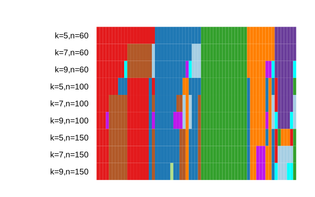
plotClusters). A few large groups persist across all nine rows, while the extra clusters for larger \(k\) split them differently depending on the genes used: the stable groups are the candidates for "tight" clusters. The cells are those shipped with clusterExperiment (the same 65 cells the book downloads with scRNAseq). Code: fig_5_13. Reproduces Holmes and Huber (2019), Figure 5.13. PDF · SVG5.5 Clustering examples: flow cytometry and mass cytometry
Section 5.5 Single-cell measurements of surface proteins make clustering concrete: flow cytometry measures about 10 markers per cell by fluorescence, mass cytometry (CyTOF) up to about 80 by mass spectrometry of metal-tagged antibodies, on hundreds of thousands of cells. Cell types correspond to combinations of high and low markers, so populations appear as dense regions in marker space.
5.5.1 Flow cytometry and mass cytometry
Section 5.5.1, Figure 5.14, Question 5.6 The markers are called CDs (clusters of differentiation); helper T cells, for instance, are CD4+. The data file Bendall_2011.fcs (Bendall et al. 2011) is read with flowCore::read.FCS. Question 5.6: it has 41 columns (39 measured channels plus the time and an event number; 38 after setting aside Time, Cell_length and absoluteEventNumber) and 91,392 cells (rows of exprs(fcsB)).
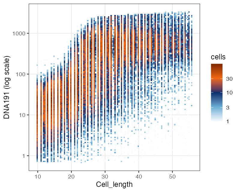
fig_5_14. Reproduces Holmes and Huber (2019), Figure 5.14. PDF5.5.2 Data preprocessing
Section 5.5.2, Figures 5.15–5.17, Question 5.7 The isotope names are replaced by marker names from Bendall_2011_markers.csv. Raw intensities are crowded near zero (and can be negative after background subtraction) with a long right tail, so they are transformed with the inverse hyperbolic sine
usually in the form \(\asinh(a+bx)\) (flowCore::arcsinhTransform(a, b); \(1/b\) is called the cofactor). The book uses \(a=0.1,b=1\) for Figure 5.15 and \(a=0,b=1\) before DBSCAN.
Filling the gap 5.7: the asinh transform is a variance-stabilising transformation Section 5.5.2
Claim. (a) \(\asinh\) is odd, increasing, \(\asinh'(x)=1/\sqrt{1+x^2}\); near 0, \(\asinh(x)=x-x^3/6+O(x^5)\); for large \(x\), \(\asinh(x)=\log(2x)+\frac{1}{4x^2}\)
So the cofactor \(1/b=\sqrt{\alpha/\beta}\) is the intensity at which multiplicative noise starts to dominate the noise floor.
Proof
(a) \(\sinh\) is odd and strictly increasing with \(\sinh'=\cosh=\sqrt{1+\sinh^2}\), so its inverse is odd, increasing, with derivative \(1/\cosh(\asinh x)=1/\sqrt{1+x^2}\). Solving \(x=(e^y-e^{-y})/2\) as a quadratic in \(e^y\) gives \(e^y=x+\sqrt{x^2+1}\) (the positive root). Integrating \((1+t^2)^{-1/2}=1-t^2/2+O(t^4)\) from 0 gives the expansion at 0. For \(x>0\), \(x+\sqrt{x^2+1}\)
(b) The delta method: if \(X\) is concentrated near \(\mu\) and \(g\) is smooth, \(g(X)\approx g(\mu)+g'(\mu)(X-\mu)\), so \(\var g(X)\approx g'(\mu)^2v(\mu)\). Requiring this to be constant, say 1, gives \(g'(\mu)=v(\mu)^{-1/2}\)
For \(\beta=0\) (pure additive noise) the limit is \(g(x)=x/\sqrt\alpha\), and for \(\alpha=0\) it is \(\log x/\sqrt\beta\) up to a constant: asinh interpolates between the identity near zero and the logarithm at large intensities. ∎
We simulate \(X=\mu+Z_1+0.1\mu Z_2\) (\(\alpha=1,\beta=0.01\)) for \(\mu\) from 0 to \(10^4\): \(\var g(X)\) stays between 0.99 and 1.03, while \(\var X\) grows by a factor \(10^6\). The same argument appears in Chapter 8 of the book for count data.
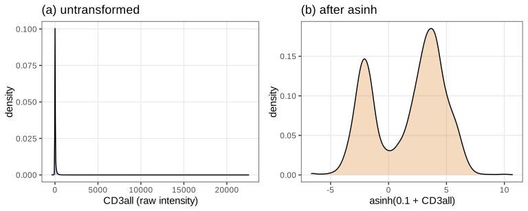
fig_5_15. Reproduces Holmes and Huber (2019), Figure 5.15. PDF · SVGQuestion 5.7 (book) asks how many dimensions kmeansFilter("CD3all" = c("Pop1", "Pop2")) uses: one, the transformed CD3all channel. Its two groups have 33,434 and 57,958 cells (36.6% and 63.4%), and plain kmeans with \(k=2\) on the same channel gives exactly these sizes. In one dimension k-means cuts at the midpoint of the two centres, which here falls in the trough between the modes of Figure 5.15(b).
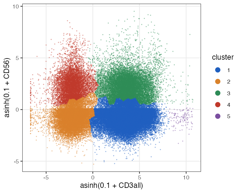
flowPeaks (sizes 45,562, 22,680, 14,969, 8,061 and 120). flowPeaks first runs k-means with many centres and then merges centres that belong to the same peak of a smoothed density, which is why its clusters need not be convex. Code: fig_5_16. Reproduces Holmes and Huber (2019), Figure 5.16. PDF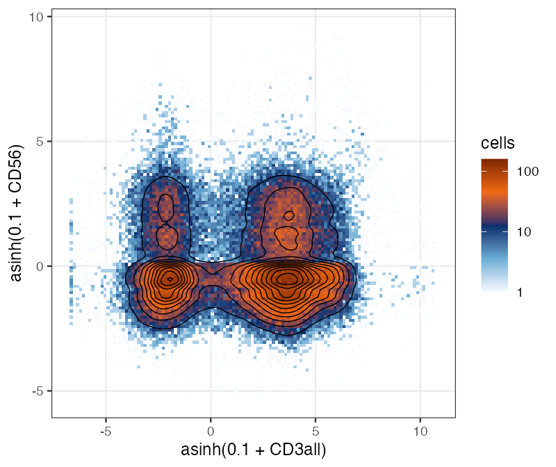
fig_5_17. Reproduces Holmes and Huber (2019), Figure 5.17. PDF5.5.3 Density-based clustering
Section 5.5.3, Figure 5.18, Question 5.8 With few markers and many cells, clusters can be defined as regions of high density separated by sparse regions. DBSCAN (Ester et al. 1996) implements this with two parameters, a radius \(\varepsilon\) and a count minPts. It finds non-convex clusters and leaves outlying points unclustered (noise). With the five markers CD4, CD8, CD20, CD3all and CD56 after \(\asinh(x)\), \(\varepsilon=0.65\) and minPts = 30, dbscan::dbscan gives 76,053 noise cells and eight clusters of 4,031, 5,450, 5,310, 257, 160, 63, 25 and 43 cells, exactly the book's table.
Definition 5.2 (the vocabulary of DBSCAN) Section 5.5.3
Let \(N_\varepsilon(p)\)
The book uses "density-connected" without defining it; the definition above is that of Ester et al. (1996).
Filling the gap 5.8: DBSCAN's clusters are connected components of the core points Section 5.5.3
Let \(G\) be the graph on the core points with an edge between core points at distance \(\le\varepsilon\).
Claim. (a) Density-reachability is reflexive and transitive but not symmetric; density-connectedness is symmetric, and on core points it is an equivalence relation. (b) The clusters of Definition 5.2 are exactly the sets \(K\cup B(K)\), where \(K\) is a connected component of \(G\) and \(B(K)\) the non-core points within \(\varepsilon\) of some point of \(K\). (c) Hence the core points of each cluster do not depend on the order in which points are processed; only a border point within \(\varepsilon\) of two components belongs to both clusters in the definition, and an implementation must pick one. (d) Every cluster contains at least minPts points in the definition, but not necessarily after an implementation has given shared border points to only one cluster.
Proof
(a) A chain of length 1 gives reflexivity and concatenating chains gives transitivity. Asymmetry: a border point \(q\) within \(\varepsilon\) of a core point \(p\) is reachable from \(p\), but nothing is reachable from \(q\) except \(q\) itself, because \(q\) is not core. Symmetry of density-connectedness is built into its definition. For core points, \(q\) directly reachable from core \(p\) means \(d(p,q)\le\varepsilon\), and then \(p\) is directly reachable from \(q\); so on core points reachability is symmetric, and "connected by a chain in \(G\)" is an equivalence relation whose classes are the components of \(G\); density-connected core points \(p,q\) (via \(o\)) lie in the component of \(o\).
(b) Let \(C\) be a cluster and \(p\in C\). Condition (i) with \(q=p\) gives a point \(o\) from which \(p\) is reachable; the chain starts at a core point. So \(C\) contains a core point \(c\), and by (ii) \(C\supseteq\) everything reachable from \(c\), which is the component \(K\) of \(c\) together with \(B(K)\) (the last link of a chain may leave the core points, but then the chain stops). Conversely every \(p\in C\) is density-connected to \(c\) via some \(o\); \(o\) is core (or \(o=p\), a core point), and since \(c\) is reachable from \(o\) through core points, \(o\in K\), so \(p\in K\cup B(K)\). Finally \(K\cup B(K)\) satisfies (i) (every point is reachable from any core point of \(K\)) and (ii) (anything reachable from a point of it is reachable from \(K\)).
(c) follows from (b). (d) A core point has at least minPts points in \(N_\varepsilon\), all reachable from it, so a cluster of the definition has at least minPts points. But dbscan::dbscan assigns each border point to the first cluster that reaches it, and a cluster can lose some of its border points to an earlier one. The book's own table shows this: with minPts = 30 one cluster has only 25 cells. So the book's third property ("groups must have at least MinPts points") is a consequence of the definition, not a rule, and it fails for the output of the implementation. In the demonstration data (CD3all and CD56, \(\varepsilon=0.3\), minPts = 15) the same happens: a cluster of 7 cells. ∎
Choosing \(\varepsilon\). A point is core exactly when its distance to its \((\text{minPts}-1)\)-th nearest other point is at most \(\varepsilon\). Plotting these distances in increasing order (the "k-distance plot", dbscan::kNNdistplot) and placing \(\varepsilon\) at the bend separates dense from sparse points (Ester et al. 1996). We compare an own implementation with dbscan::dbscan (same partition on the spirals) and verify (b) numerically.
Algorithm 5.2 (DBSCAN) Section 5.5.3; Ester et al. (1996)
- For every point compute \(N_\varepsilon(p)\) (with a spatial index this costs about \(O(n\log n)\) in low dimension) and mark the core points.
- Take the first core point not yet in a cluster, open a new cluster, and grow it by breadth-first search: add all points of \(N_\varepsilon\) of every core point already in the cluster.
- Repeat step 2 until every core point is in a cluster; label the remaining points noise.
Step 2 finds the component of Filling the gap 5.8(b), so the core points of the result are those of the definition; the border points go to the first cluster that reaches them.
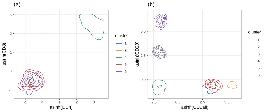
fig_5_18. Reproduces Holmes and Huber (2019), Figure 5.18. PDF · SVGQuestion 5.8 (book): adding a sixth marker (CD33) with \(\varepsilon=0.65\), minPts = 20 leaves 91,068 cells as noise and six clusters of 20 to 121 cells; with seven markers (adding CD45RA) even \(\varepsilon=0.95\) leaves 90,249 noise cells (both tables are reproduced exactly by the course code). The radius needed to keep minPts neighbours grows with the dimension: for points spread over a region of volume \(V\) in \(p\) dimensions, a ball containing a fixed number \(m\) of \(n\) points has volume about \(mV/n\), hence radius proportional to \((m/n)^{1/p}\), which approaches the size of the whole region as \(p\) grows. This is the curse of dimensionality the book refers to.
5.6 Hierarchical clustering
Section 5.6, Figures 5.19–5.26 Agglomerative hierarchical clustering starts from \(n\) singletons and merges, \(n-1\) times, the two closest clusters, recording the height of each merge. The result is a dendrogram, a binary tree with the observations as leaves (Linnaeus' taxonomy, Figure 5.19 of the book, is a hand-made hierarchy). The left-right order of the two children at each node is arbitrary (Figure 5.20, a schematic, draws one tree three ways); vertical distances carry the information. Leaves that are adjacent in the drawing need not be close in the tree. Top-down (divisive) methods split instead of merging; they reappear as decision trees in Chapter 12 of the book.
5.6.1 How to compute (dis)similarities between aggregated clusters?
Section 5.6.1, Figures 5.21–5.25, Questions 5.9–5.11 Once two clusters are merged, the algorithm needs the dissimilarity between clusters. The common linkages are
\[ d_{\text{single}}(C_1,C_2)=\min_{i\in C_1,j\in C_2}d_{ij},\quad d_{\text{complete}}(C_1,C_2)=\max_{i\in C_1,j\in C_2}d_{ij},\quad d_{\text{average}}(C_1,C_2)=\frac{1}{|C_1||C_2|}\sum_{i\in C_1,j\in C_2}d_{ij}, \]plus centroid linkage (distance between cluster means) and Ward's method (merge the pair whose union increases the within-cluster sum of squares least). Single linkage tends to chain observations into long strings and gives comb-like trees; complete linkage gives compact groups; Ward's method is the agglomerative analogue of k-means. The book's table (after Chakerian and Holmes 2012) summarises the trade-offs.
Filling the gap 5.9: the Lance-Williams recursion Section 5.6.1
After merging \(C_i\) and \(C_j\) (sizes \(n_i,n_j\)), the dissimilarity of the new cluster to any other cluster \(C_k\) (size \(n_k\)) can be computed from the old ones:
\[ d(C_i\cup C_j,C_k)=\alpha_i\,d(C_i,C_k)+\alpha_j\,d(C_j,C_k)+\beta\,d(C_i,C_j)+\gamma\,\big|d(C_i,C_k)-d(C_j,C_k)\big|, \]with (single) \(\alpha_i=\alpha_j\)
Derivation
Single and complete. \(\tfrac12(a+b)-\tfrac12|a-b|=\min(a,b)\) and \(\tfrac12(a+b)+\tfrac12|a-b|=\max(a,b)\), and the minimum over \(C_i\cup C_j\) is the smaller of the minima over \(C_i\) and over \(C_j\).
Average. The sum over \(C_i\cup C_j\) splits into the sums over \(C_i\) and \(C_j\): \(\sum_{C_i\cup C_j,C_k}d\)
Centroid. Write \(m=\frac{n_i\bar x_i+n_j\bar x_j}{n_i+n_j}\)
Ward. For two clusters the increase of \(\WSS\) on merging is \(\Delta(a,b)=\frac{n_an_b}{n_a+n_b}|\bar x_a\)
Starting from the matrix of \(d_{ij}\) (or \(d_{ij}^2\) for centroid and Ward), the whole tree is thus computed by repeated "find the smallest entry, update one row", which is how hclust works; its ward.D2 option squares the input and reports \(\sqrt{D}\). We implement the recursion and reproduce hclust's merge heights for all five linkages to \(10^{-9}\); the hierarchical-clustering demo uses the same recursion.
Filling the gap 5.10: dendrograms are ultrametrics, single linkage is a minimum spanning tree, centroids can invert Section 5.6.1, Figure 5.11
Let \(h_1,h_2,\dots,h_{n-1}\) be the merge heights and define the cophenetic distance \(c(x,y)\) as the height of the merge at which \(x\) and \(y\) first fall into the same cluster.
Claim. (a) For single, complete, average and Ward linkage the heights never decrease, \(h_1\le h_2\le\cdots\). (b) If the heights never decrease, \(c\) is an ultrametric (Definition 5.1). (c) The single-linkage heights are the edge lengths of a minimum spanning tree of the complete graph with weights \(d_{ij}\), and cutting the single-linkage tree at height \(h\) gives the connected components of the graph with edges \(d_{ij}\le h\). (d) Centroid linkage can produce an inversion \(h_{s+1}<h_s\). (e) A dendrogram with \(n\) leaves can be drawn with \(2^{n-1}\) leaf orders (Question 5.11: \(2^{10}=1024\) for the 11 leaves of Figure 5.26).
Proof
(a) A linkage is called reducible if merging \(C_i,C_j\) at the current minimum \(\delta=d(C_i,C_j)\) cannot create a cluster closer to some \(C_k\) than \(\delta\): \(d(C_i\cup C_j,C_k)\ge\delta\) whenever \(d(C_i,C_k),d(C_j,C_k)\ge\delta\). Then the minimum of the updated matrix is again \(\ge\delta\), so the next height is at least \(\delta\). Single: \(\min(a,b)\ge\delta\). Complete: \(\max(a,b)\ge\delta\). Average: a weighted mean of numbers \(\ge\delta\). Ward: by the recursion \((n_i+n_j+n_k)D_{\text{new}}\)
(b) Take \(x,y,z\) and let \(t=\max\{c(x,y),c(y,z)\}\). After the merge at height \(t\) (heights are ordered), \(x\) and \(y\) are in one cluster and \(y\) and \(z\) are in one cluster; clusters are disjoint, so all three are together and \(c(x,z)\le t\). The other metric properties are clear (\(c(x,y)=0\) only for \(x=y\) if all \(d_{ij}>0\)).
(c) Single linkage merges the two clusters joined by the shortest edge between different clusters. This is exactly Kruskal's algorithm for a minimum spanning tree (add the shortest edge that joins two different components), so the merges correspond to tree edges and the heights to their lengths. Two points are in the same cluster at height \(h\) iff they are linked by a chain of edges of length \(\le h\).
(d) Three points at the vertices of an equilateral triangle with side 1: the first merge is at height 1 (squared distance 1); the centroid of the merged pair is at distance \(\sqrt3/2\approx0.87<1\) from the third point, so the second merge is lower. In the bridge data of the demonstration, centroid linkage gives two inversions, as in hclust.
(e) A binary tree with \(n\) leaves has \(n-1\) internal nodes, and each can independently exchange its two subtrees; distinct sets of exchanges give distinct leaf orders because the leaves are distinct (the first node, from the root, at which two exchange sets differ puts different leaves first). So there are \(2^{n-1}\) orders. ∎
We verify (a) and (b) on the Morder data for four linkages, (c) against Prim's algorithm, the inversions in (d), and (e) by enumerating all orders of a 6-leaf tree (32).
Filling the gap 5.11: what Ward's method minimises Section 5.6.1, Figure 5.23
Claim. Merging clusters \(A\) and \(B\) increases the within-cluster sum of squares by
\[ \Delta(A,B)=\WSS(A\cup B)-\WSS(A)-\WSS(B)=\frac{n_An_B}{n_A+n_B}\,|\bar x_A-\bar x_B|^2, \]so Ward's method merges, at each step, the pair with the smallest increase of the total \(\WSS\); hclust(method = "ward.D2") reports the height \(\sqrt{2\Delta}\).
Proof
Let \(m\) be the mean of \(A\cup B\). By the decomposition of Filling the gap 5.5(a), \(\WSS(A\cup B)\)
The greedy merges do not in general give the partition with the smallest \(\WSS\) for a given \(k\) (that is the k-means problem), but they often give a good start for k-means. The formula holds on the last merge of the bridge data.
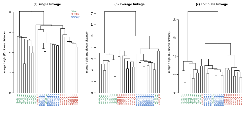
Morder (Euclidean distance; labels coloured naive, effector, memory). Single linkage gives the comb-like tree with long chains of single merges; average and complete linkage both separate three groups that match the cell types closely (cut at three clusters: 9 naive, 9 effector, and a group of 9 memory with 1 effector and 2 naive cells) and differ mostly in the heights of the inner branches. The book draws this figure from a small distance matrix (d14) that is not distributed; it is re-created here on the Morder data of the same section. Code: fig_5_25. Reproduces Holmes and Huber (2019), Figure 5.25. PDF · SVGQuestions 5.9 and 5.10 (book) ask for heatmaps of the Euclidean and Manhattan distance matrices of Morder, first in the original order and then reordered by the hierarchical clustering trees. In the original order (samples grouped by patient) little structure is visible; reordered by the tree, three blocks appear along the diagonal, one per cell type. The two distances give very similar trees: cutting the average-linkage trees into three clusters gives an adjusted Rand index of 0.89 between the Euclidean and the Manhattan partitions, and the Manhattan tree puts all 10 effector samples together (the Euclidean one 9 of 10). The demonstration, presets 6 and 7 shows both reordered heatmaps.
Question 5.11 (book): the tree of Figure 5.26 (a schematic with 11 leaves) can be drawn with \(2^{10}=1024\) leaf orders consistent with it (Filling the gap 5.10(e)). This freedom is why a heatmap ordered by a tree can make clusters look stronger than they are; seriation methods choose among these orders, or use other orderings altogether.
5.7 Assessing the quality of a clustering result; choosing the number of clusters
Section 5.7, (5.7), (5.8), Figures 5.27–5.29, Questions 5.12–5.14 Clustering methods always deliver groups, so they must be validated. A first criterion is compactness, the within-groups sum of squared distances
\[ \WSS_k=\sum_{\ell=1}^k\sum_{x_i\in C_\ell}d^2(x_i,\bar x_\ell). \tag{5.7} \]\(\WSS_k\) alone cannot choose \(k\): the optimal value decreases in \(k\) and is 0 for \(k=n\). One looks instead for an elbow, a \(k\) after which the decrease becomes small, or calibrates \(\WSS_k\) against data without clusters (the gap statistic, Section 5.7.1). The test data are 400 points from four normal groups with standard deviation 2 centred at \((0,0),(0,8),(8,0),(8,8)\) (Figure 5.27).
Filling the gap 5.12: two forms of WSS, the decomposition TSS = WSS + BSS, and the Calinski-Harabasz index Section 5.7, (5.7), (5.8), Questions 5.12, 5.14
Claim. For Euclidean \(d\): (a) Question 5.12, the pairwise form
\[ \WSS_k=\sum_{\ell=1}^k\frac{1}{2n_\ell}\sum_{x_i\in C_\ell}\sum_{x_j\in C_\ell}d^2(x_i,x_j). \tag{5.8} \](b) \(\TSS=\WSS_k+\BSS_k\), where \(\TSS=\sum_i|x_i-\bar x|^2\) and \(\BSS_k=\sum_\ell n_\ell|\bar x_\ell\)
the \(F\) statistic of a one-way analysis of variance of the data on the cluster labels (summed over coordinates); a large value means well separated, compact clusters.
Proof
(a) Fix a cluster with mean \(m\) and write \(x_i-x_j=(x_i-m)-(x_j-m)\). Then \(\sum_{i,j}|x_i-x_j|^2\)
(b) Apply the decomposition of Filling the gap 5.5(a) with all \(c_\ell=\bar x\): \(\sum_i|x_i-\bar x|^2\)
(c) An optimal \(k\)-partition can be refined into a \((k+1)\)-partition by splitting off one point of a cluster with at least two points into its own cluster; splitting never increases \(\WSS\) (each part is measured about its own, optimal, mean), so the optimum over \((k+1)\)-partitions is at most the \(k\) optimum.
(d) In a one-way ANOVA with \(k\) groups and \(n\) observations the between and within mean squares have \(k-1\) and \(n-k\) degrees of freedom, and \(F\) is their ratio; with \(p\) coordinates the sums of squares add over coordinates. ∎
Erratum. The book prints \(\CH(k)=\frac{\BSS_k}{\WSS_k}\times\frac{N-k}{N-1}\). The correct factor is \(\frac{N-k}{k-1}\), which is what fpc::calinhara (used for Figure 5.29) computes: on the simulation with PAM and \(k=4\), calinhara gives 584.15, the printed formula 4.39, and their ratio is exactly \((N-1)/(k-1)=133\). With the printed factor the index would not even depend on \(k\) through the degrees of freedom of the between-group term.
We verify (5.7) = (5.8), \(\TSS=\WSS+\BSS\) and the calinhara formula on the simulation.
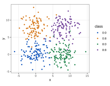
fig_5_27. Reproduces Holmes and Huber (2019), Figure 5.27. PDF · SVG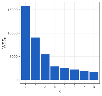
fig_5_28. Reproduces Holmes and Huber (2019), Figure 5.28. PDF · SVG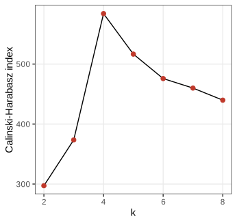
fig_5_29. Reproduces Holmes and Huber (2019), Figure 5.29. PDF · SVGQuestion 5.13 (book). Repeated runs of kmeans with one random start give different \(\WSS_k\) for \(k\ge5\) (for \(k=5\), six runs gave 2,527, 2,578, 2,525, 2,525, 2,528, 2,564), because Lloyd-type algorithms stop at local minima (Filling the gap 5.5); with many starts the values stabilise. For 400 uniform points on the same rectangle, \(\WSS_k\) falls smoothly (24,342, 13,695, 9,055, 5,966, 4,858, 4,120, 3,511, 2,927): there is no elbow, and yet k-means returns \(k\) groups for every \(k\) (demo, preset 7). For uniform data in \(p\) dimensions the optimal \(\WSS_k\) decreases roughly like \(k^{-2/p}\), a power law without a kink (Tibshirani et al. 2001), which is the shape the gap statistic uses as its reference.
5.7.1 Using the gap statistic
Section 5.7.1, Figures 5.30, 5.31, Questions 5.15, 5.16 Tibshirani, Walther and Hastie (2001) compare \(\log W_k\) with its expectation under a reference distribution without clusters, estimated by simulation.
Algorithm 5.3 (the gap statistic) Section 5.7.1; Tibshirani et al. (2001)
- Cluster the data for \(k=1,\dots,K\) and compute \(W_k\) for each clustering.
- Draw \(B\) reference data sets of the same size, uniformly over a box containing the data: either the bounding box of the original coordinates, or the bounding box in the principal-component coordinates of the centred data, mapped back (
spaceH0 = "scaledPCA", the default ofclusGap). Cluster each and compute \(W^*_{kb}\). - Compute \(\bar l_k=\frac1B\sum_b\log W^*_{kb}\), \(\gap(k)=\bar l_k-\log W_k\), \(\sd_k\) the standard deviation of the \(\log W^*_{kb}\), and \(s_k=\sd_k\sqrt{1+1/B}\).
- Choose \(k\): Tibs2001SEmax, the smallest \(k\) with \(\gap(k)\ge\gap(k+1)-s_{k+1}\); or firstSEmax (the default of
maxSE), the smallest \(k\) with \(\gap(k)\ge\gap(\hat k)-s_{\hat k}\), where \(\hat k\) is the first local maximum of the gap.
Filling the gap 5.13: what clusGap computes, why uniform references, and where \(\sqrt{1+1/B}\) comes from Section 5.7.1
(a) The quantity \(W_k\). The book describes the gap statistic with \(\WSS_k\). cluster::clusGap computes \(W_k=\sum_\ell\frac{1}{2n_\ell}\sum_{i<j\in C_\ell}d_{ij}^{\,q}\) with d.power \(=q\). Its default is \(q=1\), plain (unsquared) Euclidean distances, so the book's code does not use \(\WSS_k\) at all. With \(q=2\), the sum over unordered pairs gives \(W_k=\WSS_k/2\) by (5.8); the factor 1/2 cancels in the gap. Both versions are legitimate (Tibshirani et al. use \(q=2\)), but they can choose different \(k\): on the simulation with \(q=2\), clusGap gives \(\gap(1)=0.464\ge\gap(2)-s_2=0.440\), so the Tibs2001SEmax rule stops at \(k=1\) although the four groups are obvious (firstSEmax still gives 4; demo, preset 5).
(b) Why a uniform reference. Tibshirani et al. (2001) argue that, in one dimension, the uniform is the unimodal distribution most likely to produce spurious clusters, so calibrating against it is conservative; aligning the box with the principal axes makes the reference respect the shape of the data cloud. The reference also accounts for the fact that \(\log W_k\) decreases with \(k\) even without clusters (roughly \(-\tfrac2p\log k\) for uniform data), so the gap isolates the extra decrease due to structure.
(c) The standard error \(s_k=\sd_k\sqrt{1+1/B}\). The gap compares \(\log W_k\) of the data with \(\bar l_k\). Treat \(\log W_k\) as one more draw from the reference distribution (the null hypothesis of no clusters), independent of the \(B\) reference draws, with variance \(\sigma_k^2\). Then \(\var(\bar l_k-\log W_k)\)clusGap uses the divisor \(B-1\) in \(\sd_k\), Tibshirani et al. the divisor \(B\); the difference is negligible.)
(d) The rules. Tibs2001SEmax stops at the first \(k\) whose gap is within one standard error of the next one: adding a cluster does not improve the fit beyond the simulation noise. firstSEmax first finds the first local maximum \(\hat k\) and then takes the smallest \(k\) whose gap is within one standard error of \(\gap(\hat k)\).
Erratum. The book describes firstSEmax as "the first value of \(k\) for which the gap is not larger than the first local maximum minus a standard error"; it should read "not smaller": the rule picks the smallest \(k\) with \(\gap(k)\ge\gap(\hat k)-s_{\hat k}\) (see the code of maxSE). The book also says that Tibshirani et al. recommend "bootstrap resampling" for the gap statistic; the \(B\) reference sets are Monte Carlo draws from a null distribution, not resamples of the data.
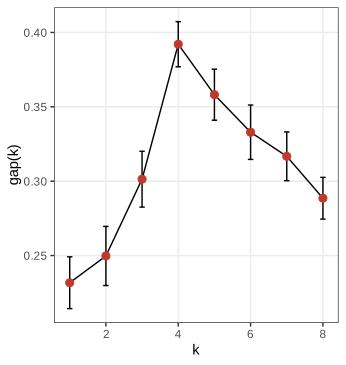
d.power = 1), with \(\pm s_k\) bars: it peaks at \(k=4\), and both rules choose 4. Code: fig_5_30. Reproduces Holmes and Huber (2019), Figure 5.30. PDF · SVGQuestion 5.15 asks for the plotting function behind Figure 5.30: a line through \(\gap(k)\) with error bars \(\gap(k)\pm s_k\) (the course code's plot_gap). For the Hiiragi embryo data the book clusters the 101 cells on the 50 most variable probes, with \(K=24\).
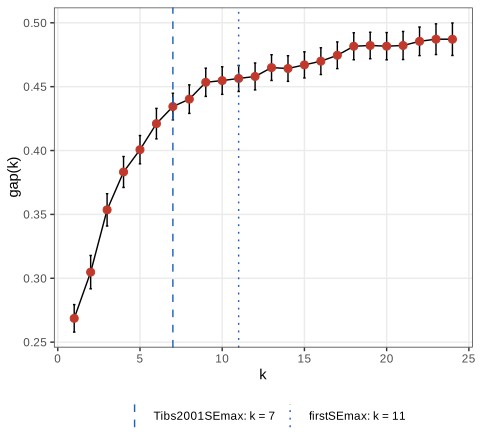
fig_5_31. Reproduces Holmes and Huber (2019), Figure 5.31. PDF · SVGCross-tabulating the PAM clusters (with the \(k\) chosen in this run) against the known sample groups shows that the clusters follow the embryonic stage and genotype: the E4.5 EPI, E4.5 PE and E4.5 FGF4-KO cells each form their own cluster, the E3.5 FGF4-KO cells form one cluster, and the E3.25 cells spread over three clusters, as in the book's table.
Question 5.16 (book): using all 45,101 probes instead of the 50 most variable ones. With all probes (PAM, clusGap with \(B=10\) because each reference set now has 45,101 columns) the gap rises to a maximum at \(k=7\) and both rules choose \(k=6\). The clusters still isolate the three E4.5 groups and the E3.25 FGF4-KO cells, but the E3.5 epiblast, primitive endoderm and FGF4-KO cells all fall into one cluster together with 19 of the 36 E3.25 wild-type cells: the E3.5 lineage split, which is carried by a few strongly varying genes, is drowned by the accumulated small variation (technical and batch effects included) of tens of thousands of weakly expressed probes. This is the reason for the feature selection step in the book.
5.7.2 Cluster validation using the bootstrap
Section 5.7.2, Figures 5.32, 5.33 The ideal check of a clustering is to redo it on new samples from the same population (Figure 5.32(a), a schematic); resampling the data imitates this (Figure 5.32(b)). The book tests the hypothesis that the inner cell mass at E3.5 splits into two groups (epiblast and primitive endoderm) while E3.25 does not. For each day separately, 250 times: draw 67% of the wild-type cells without replacement, select the 50 most variable probes in the subsample, cluster the subsample with PAM into \(k=2\) groups, and predict the cluster of every cell by its nearest medoid. Then compute a consensus clustering of the 250 partitions and the agreement of each partition with the consensus (package clue, Hornik 2005).
Erratum. The book's description says that step 3 "applies \(k\)-means clustering", but the function it shows calls pam (k-medoids).
Filling the gap 5.15: comparing partitions when the labels are arbitrary Section 5.7.2
Represent a partition of \(n\) objects into \(k\) classes by its \(n\times k\) membership matrix \(U\) (rows sum to one; for a hard partition each row is a unit vector). Cluster labels are arbitrary, so two partitions \(U,V\) are compared up to a permutation \(\Pi\) of the columns:
\[ d(U,V)=\min_{\Pi}\|U-V\Pi\|_F. \]Claim. (a) Computing \(d\) is a linear assignment problem: \(\|U-V\Pi\|_F^2\)
Proof
(a) Permuting columns does not change \(\|V\|_F\), and \(\langle U,V\Pi\rangle_F\)
The consensus partition of an ensemble is a partition (possibly soft) that minimises the sum of squared distances \(d\) to all members (cl_consensus); its memberships are the "probabilities" in the right panel of Figure 5.33. A sample whose consensus membership is near 1/2 is assigned inconsistently across resamples.
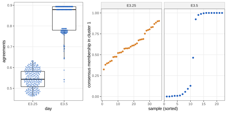
fig_5_33. Reproduces Holmes and Huber (2019), Figure 5.33. PDF · SVGFilling the gap 5.16: model-based clustering and the BIC Sections 5.4, 5.7; Chapter 4
The parametric alternative to the methods of this chapter is the normal mixture of Chapter 4, \(f(x)=\sum_{m=1}^k\pi_m\phi(x;\mu_m,\Sigma_m)\), fitted by EM for each \(k\) and for several covariance structures (mclust), with \(k\) chosen by the Bayesian information criterion
where \(\nu\) is the number of free parameters (\(k-1\) weights, \(kp\) means and the covariance parameters).
Why BIC. For a model \(M\) with prior \(\pi(\theta)\), the marginal likelihood \(p(\text{data}\given M)\)
Relation to k-means. With equal weights and \(\Sigma_m=\sigma^2I\), classifying each point to its most likely component and maximising the "classification likelihood" over labels and means is exactly minimising \(\WSS\) (k-means); the small-variance limit of Filling the gap 5.5 is the same statement for EM.
On the simulation, Mclust with \(k=1,\dots,8\) chooses 4 components and its partition agrees with PAM's (adjusted Rand index above 0.9); we also confirm \(\mathrm{BIC}=2\log\hat L-\nu\log n\) for the chosen model.
5.8 Clustering as a means for denoising
Section 5.8 When observations are noisy copies of a few true values (sequence variants with sequencing errors), clustering recovers the true values as cluster centres, and the cluster sizes estimate their abundances.
5.8.1 Noisy observations with different baseline frequencies
Section 5.8.1, Figures 5.34, 5.35, Question 5.17 Two "sequences" with the same bivariate normal noise, \(\N(\mu_g,0.5I)\) with \(\mu_1=(-1,-1)\), \(\mu_2=(1,1)\), but with \(10^3\) copies of seq1 and \(10^5\) of seq2 (Figure 5.34). Because the abundant group has 100 times more draws, its extreme draws reach much further, and its apparent radius is larger.
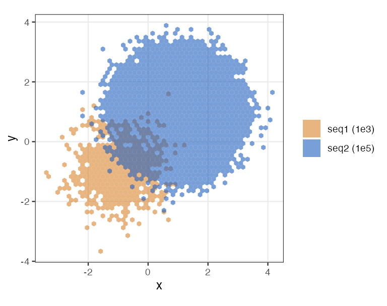
fig_5_34. Reproduces Holmes and Huber (2019), Figure 5.34. PDFFilling the gap 5.17: unequal abundances move the boundary Section 5.8.1, Question 5.17
Claim. For two groups \(\N(\mu_1,\sigma^2I)\) and \(\N(\mu_2,\sigma^2I)\) with prior proportions \(\pi_1,\pi_2\), the posterior probabilities are equal on the hyperplane perpendicular to \(\mu_2-\mu_1\) at signed distance
\[ t=\frac{\sigma^2\log(\pi_2/\pi_1)}{|\mu_2-\mu_1|} \]from the midpoint, towards the rare group (if \(\pi_2>\pi_1\), towards \(\mu_1\)). The "nearest centre" rule, which uses \(t=0\), is the Bayes rule only for equal abundances.
Proof
The posterior odds are \(\frac{\pi_2\phi(x;\mu_2)}{\pi_1\phi(x;\mu_1)}\), and the log odds are \(\log\frac{\pi_2}{\pi_1}\)
Numbers for Figure 5.34. \(\sigma^2=0.5\), \(|\mu_2-\mu_1|=2\sqrt2\), \(\pi_2/\pi_1=100\): \(t=0.5\log100/(2\sqrt2)=0.814\). The projection of a seq2 draw on \(u\) is \(\N(\sqrt2,0.5)\) about the midpoint. Under the nearest-centre rule a fraction \(\Prob(Z>2)=0.0228\) of seq2 draws, about 2,275 reads, fall on seq1's side: more than twice the 1,000 true seq1 reads, so the "seq1 cluster" would be mostly errors of seq2. Under the Bayes rule only about 81 seq2 reads cross, at the price of assigning about 198 of the 1,000 seq1 reads to seq2. Abundance is information, which is why distance-only (OTU) clustering is biased and DADA2 models abundances (Section 5.8.3). The shift is verified by root-finding.
The book's Task simulates 2,000 reads of length 200 with independent errors at rate 0.001 and computes the diameter (the largest pairwise number of mismatches) of random subsets of increasing size (Figure 5.35).
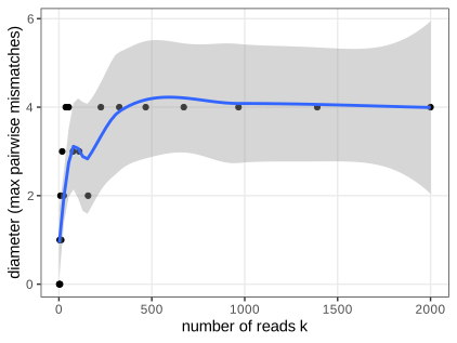
fig_5_35. Reproduces Holmes and Huber (2019), Figure 5.35. PDF · SVGFilling the gap 5.18: errors per read, and why the diameter grows Section 5.8.1, Question 5.18, Figures 5.35, 5.36
Claim. (a) With independent errors at rate \(p\) at each of \(L\) positions, the number of errors in a read is \(\Bin(L,p)\), and the total variation distance to \(\Pois(Lp)\) is at most \(Lp^2\) (Le Cam's inequality). (b) The number of mismatches between two reads is \(\Bin(L,2p(1-p))\), with mean \(2Lp(1-p)\). (c) The diameter of \(k\) reads grows with \(k\) without bound in distribution: it is the maximum of \(k(k-1)/2\) dependent mismatch counts, and \(\Prob(\text{some read has}\)
Proof
(a) A sum of \(L\) independent Bernoulli variables with equal \(p\) is binomial. Le Cam's inequality, \(\sum_r|\Prob(S\)
(b) Two reads differ at a position when exactly one of them has an error there (the book's TRUE/FALSE encoding records only whether a base is correct, so two errors at the same position count as a match): probability \(2p(1-p)\), independently over positions. For \(L=200,p=0.001\) the mean is 0.3996, as the simulation confirms.
(c) The diameter is at least the largest number of errors of a single read (compare it with an error-free read, which exists with high probability since \(\Prob(0\text{ errors})\)
Erratum (Question 5.18). The question states that errors are Bernoulli(0.0005) events, but its solution says that "the sum of 200 independent Poisson(0.0005) will be Poisson(0.1)" and the code simulates Poisson errors. The sum of Poisson variables is exactly Poisson, but the number of Bernoulli errors is \(\Bin(200,0.0005)\); Poisson(0.1) is an approximation, excellent here by (a).
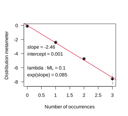
vcd::distplot) of \(10^5\) simulated error counts per read (sums of 200 Poisson(0.0005)): the points lie on a line, the estimated rate is 0.1. Code: fig_5_36. Reproduces Holmes and Huber (2019), Figure 5.36. PDF · SVGQuestion 5.17 (book): yes, a clustering by distance to the group centres depends on the frequencies, and should: Filling the gap 5.17 shows how much. The book connects the distance-only rule with the "representativeness" heuristic of Tversky and Kahneman (1974), which ignores base rates.
5.8.2 Denoising 16S rRNA sequences
Section 5.8.2 Amplicon sequencing of the variable regions of the bacterial 16S rRNA gene produces reads (FASTQ files with a quality score per base) from which one wants the exact amplicon sequence variants (ASVs) present and their counts per sample. The approach is de novo: an error model is estimated from the data themselves, alternating between assigning reads to candidate true sequences and re-estimating error rates (an EM-like scheme), and the cluster centres are the denoised variants (Callahan et al. 2016, 2017). The preprocessing steps (quality inspection, trimming, filtering, dereplication) are Exercises 5.5 to 5.7.
5.8.3 Infer sequence variants
Section 5.8.3, Figure 5.37, Questions 5.19, 5.20 DADA (Rosen et al. 2012) models substitution errors by probabilities \(p(b\to b'\given q)\) of reading base \(b'\) when the true base is \(b\), as a function of the quality score \(q\), assumed independent of position. They are estimated from the data by alternating denoising and estimation (dada(..., selfConsist = TRUE)).
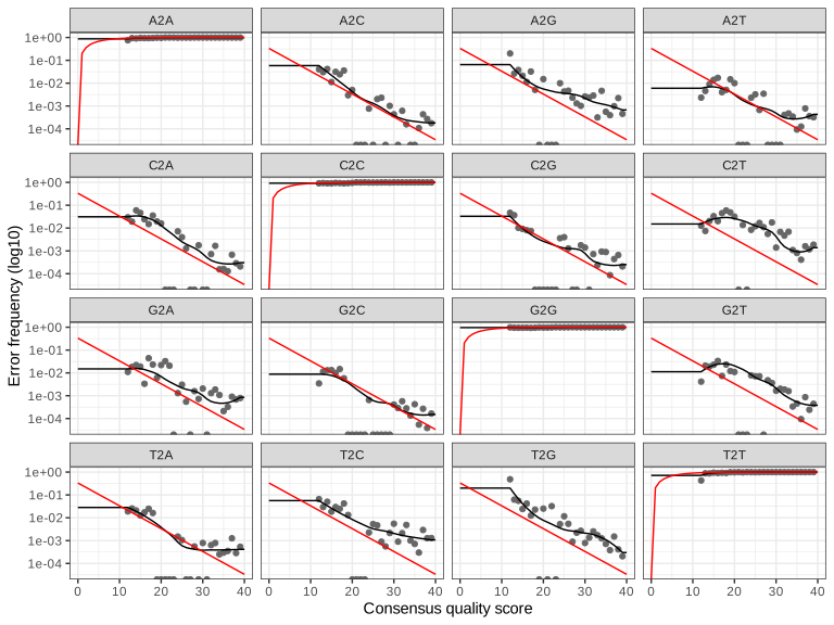
plotErrors): one panel per transition (true base to read base); points are observed frequencies, black lines the fitted rates, red lines the rates implied by the nominal quality scores \(10^{-q/10}\). Off-diagonal rates fall with quality as they should; the diagonal panels are the probabilities of a correct call. Code: fig_5_37 (the run takes about 15 minutes and is cached). Reproduces Holmes and Huber (2019), Figure 5.37. PDF · SVGFilling the gap 5.19: the abundance p-value of DADA Section 5.8.3; Rosen et al. (2012), Callahan et al. (2016)
Let a candidate true sequence \(j\) have \(n_j\) reads, and let \(i\) be a different unique sequence observed \(a_i\) times. Under the error model, the probability that a read of \(j\) comes out as \(i\) is \(\lambda_{ji}=\prod_{\text{positions }s}p(j_s\to i_s\given q_s)\), the product of transition probabilities (independence across positions). If all reads of \(i\) were errors of \(j\), their number would be \(N\sim\Bin(n_j,\lambda_{ji})\)
A small \(p_i\) means that \(i\) is too abundant to be explained by errors of \(j\), and \(i\) becomes a new cluster centre (a new variant); the algorithm splits clusters until no such sequence remains (with a multiple-testing-adjusted threshold), then re-estimates the error rates. This is the formal version of Filling the gap 5.17: a sequence 1 mismatch away from a very abundant one is expected by error; the same sequence next to a rare one is not.
After denoising, read pairs are merged (mergePairs), a table of ASV counts per sample is made (makeSequenceTable), and chimeras are removed (removeBimeraDenovo). Question 5.19: dadaRs (and dadaFs) is a list of 20 dada objects, one per sample (19 mouse samples and the mock community), each holding the denoised variants, their abundances and the read-to-variant assignment; mergers is a list of 20 data frames of merged sequences with their abundances. Question 5.20: a chimera is a read made of the first part of one true sequence and the rest of another (PCR switching templates); it is easy to recognise because it is an exact concatenation of a prefix and a suffix of two more abundant variants in the same sample, which can be checked exhaustively. In this run the table has 427 ASVs before and 277 after chimera removal, so 150 of 427 variants (35%) were chimeric, but they account for only 7.2% of the reads (the book: 7%), because chimeras are individually rare.
5.9 Computational and memory issues
Section 5.9 An algorithm is \(O(n^k)\) if its cost grows proportionally to \(n^k\) for large \(n\).
Filling the gap 5.20: costs of the methods of this chapter Section 5.9
- Distance matrix: \(n(n-1)/2\) entries, \(O(n^2p)\) time. For \(n=10^6\) and 8-byte numbers: \(\approx5\times10^{11}\times8\) bytes \(=4\times10^{12}\) bytes, the book's 4 terabytes.
- Naive agglomeration (search the whole matrix for the minimum at each of \(n-1\) steps): \(O(n^3)\) time; \(10^{18}\) operations at one nanosecond each is \(10^9\) seconds, about 31.7 years, the book's "30 years". Better algorithms reach \(O(n^2)\) time for single linkage (via the minimum spanning tree, Filling the gap 5.10(c)) and for the reducible linkages of Filling the gap 5.10(a) by the nearest-neighbour-chain algorithm (Müllner 2013).
- k-means: each Lloyd iteration costs \(O(nkp)\) and \(O(n+k)\) memory beyond the data, linear in \(n\); the number of iterations is usually small.
- PAM: \(O(n^2)\) memory for the distance matrix and \(O(n^2)\) per SWAP step with the formula of Filling the gap 5.6; for large \(n\), CLARA runs PAM on subsamples.
- DBSCAN: one range query per point; with a spatial index in low dimension about \(O(n\log n)\), \(O(n^2)\) in the worst case.
Summary
- The distance is the first and most consequential choice. Minkowski distances with \(m\ge1\), Mahalanobis, Jaccard, correlation and edit distances are metrics (or pseudometrics); the Mahalanobis distance is Euclidean after whitening.
- Partitioning methods (k-means, k-medoids, PAM) decrease their objective at every step and stop at local optima; k-means is the hard, small-variance limit of EM; PAM's swap-optimality is stronger than the alternating algorithm's.
- Cytometry data need a variance-stabilising transformation, asinh; DBSCAN's clusters are the connected components of the core points, with border points attached, and need not have minPts points in implementations.
- Hierarchical clustering is driven by the Lance-Williams recursion; monotone linkages give ultrametric trees; single linkage is the minimum spanning tree; Ward merges by the smallest increase of \(\WSS\).
- \(\WSS_k\) has a pairwise form and decomposes \(\TSS\); the Calinski-Harabasz index is an \(F\) ratio with factor \((n-k)/(k-1)\); the gap statistic calibrates \(\log W_k\) against uniform reference data with standard error \(\sd_k\sqrt{1+1/B}\), and its rules can disagree; silhouettes and resampling stability complete the picture, and the BIC chooses \(k\) for parametric mixtures.
- Distances are not everything: abundances shift the Bayes boundary towards rare groups, and error models with abundance p-values (DADA2) denoise reads better than distance thresholds.
Exercises
The eight exercises of Chapter 5 (Holmes and Huber 2019, Section 5.12), restated in my own words, with solutions (hidden). Numerical answers come from the course code.
Exercise 5.1 (silhouettes). For a point \(x_i\) let \(a(i)\) be its average dissimilarity to the other members of its own cluster and \(b(i)\) the smallest average dissimilarity to the members of another cluster (the "neighbouring" cluster). The silhouette index is \(s(i)=\frac{b(i)-a(i)}{\max\{a(i),b(i)\}}\). Compute the silhouettes of a PAM clustering of the four-group simulation with \(k=4\), find the \(k\) with the best average silhouette, and repeat for uniform data.
Solution
Filling the gap 5.14: properties of the silhouette Exercise 5.1; Rousseeuw (1987)
Claim. (a) \(-1\le s(i)\le1\); \(s(i)>0\) iff \(a(i)<b(i)\), i.e. iff \(x_i\) is on average closer to its own cluster than to any other. (b) \(s(i)=1-a(i)/b(i)\) if \(a(i)\le b(i)\) and \(s(i)=b(i)/a(i)-1\) otherwise. (c) For a singleton cluster \(a(i)\) is undefined and \(s(i)\) is set to 0 by convention.
Proof
If \(a\le b\) then \(\max=b\) and \(s=(b-a)/b=1-a/b\in[0,1]\) since \(0\le a/b\le1\). If \(a>b\) then \(s=(b-a)/a=b/a-1\in[-1,0)\). Both cases give (a) and (b); \(s=1\) requires \(a=0\) (members at distance 0 from each other), \(s=-1\) requires \(b=0\). ∎
Erratum. The book writes the denominator as \(\max_i(A(i),B(i))\); the maximum is over the two numbers for the same \(i\), not over \(i\) (with a maximum over all points the index would lose its \([-1,1]\) scaling point by point). We reproduce
cluster::silhouettewith the formula above.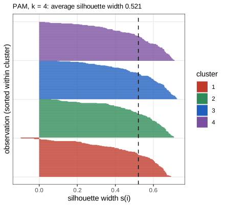
Silhouette plot for Exercise 5.1. PAM with \(k=4\) on the simulation; bars are \(s(i)\), sorted within clusters; the dashed line is the average, 0.521. A few points between groups have \(s(i)\) near 0. (The book computes but does not show this plot.) Code: fig_5_ex1. PDF · SVGAverage silhouette by \(k\) (PAM, Euclidean):
k 2 3 4 5 6 7 8 four groups 0.409 0.452 0.521 0.471 0.423 0.380 0.366 uniform 0.391 0.404 0.409 0.395 0.392 0.372 0.352 The silhouette picks \(k=4\) for the simulation. On uniform data it is flat around 0.4 and still has a (meaningless) maximum: an average silhouette of 0.4 does not prove that clusters exist, because partitioning a uniform cloud into convex cells already makes points closer to their own cell. Silhouettes compare values of \(k\) but, unlike the gap statistic, have no built-in reference for \(k=1\). (Demo, preset 6.)
Exercise 5.2. For the 20 sites of the
dunevegetation data (package vegan), make a character representation of their distance matrix withsymnum, and a heatmap of the distances.Solution
Compute the Bray-Curtis dissimilarities \(d_{ij}=\sum_s|y_{is}-y_{js}|/\sum_s(y_{is}\)
\({}+y_{js})\) (the default of vegdist, suited to species abundances; it lies in [0, 1] and ignores joint absences):d <- vegan::vegdist(dune). On these data the 190 dissimilarities range from 0.23 to 1.00 (median 0.65). Thensymnum(as.matrix(d), cutpoints = c(0, 0.25, 0.5, 0.75, 1), symbols = c(" ", ".", "+", "*"))prints the matrix with one symbol per interval, which shows blocks of similar sites at a glance. For the heatmap, order the sites by a hierarchical clustering ofd, e.g.pheatmap(as.matrix(d), clustering_distance_rows = d, clustering_distance_cols = d); passing the dissimilarity object makes the dendrograms use Bray-Curtis instead of the Euclidean default. Note that Bray-Curtis is not a metric (the triangle inequality can fail), which matters for methods that assume one (classical MDS, Chapter 9 of the book), not for hierarchical clustering.Exercise 5.3. Cluster the
spiralsdata (package kernlab) with k-means; then cluster them with a method that can follow the arms (speccordbscan), and study how robust the number of groups found bydbscanis to its parameters.Solution
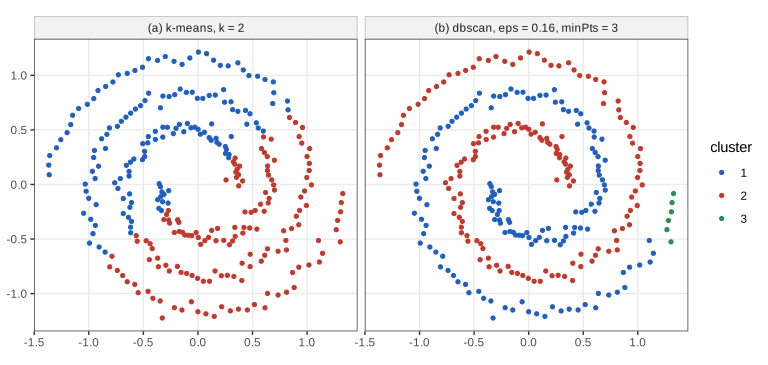
Figure 5.38. (a) k-means with \(k=2\) cuts the two spirals by a line (its clusters are convex cells). (b) DBSCAN with \(\varepsilon=0.16\), minPts = 3 follows the arms: clusters of 150 and 144 points, and a third cluster of 6 points at the end of one arm. Code: fig_5_38. Reproduces Holmes and Huber (2019), Figure 5.38. PDF · SVGk-means cannot succeed for any start: each cluster is an intersection of half-spaces, and no convex set contains one spiral arm without points of the other. DBSCAN works because the arms are chains of points closer than \(\varepsilon\) to each other while the gap between arms is wider. Robustness, with minPts = 3:
\(\varepsilon\) 0.08 0.10 0.12 0.14 0.16 0.18 \(\ge0.20\) clusters 31 19 11 6 3 2 1 noise points 84 14 2 1 0 0 0 So the "right" answer holds only in a narrow window, \(0.16\le\varepsilon<0.20\): too small and the arms break into pieces, too large and \(\varepsilon\) bridges the arms. With \(\varepsilon=0.16\), minPts = 5 gives 5 clusters and 24 noise points, minPts = 8 gives 3 clusters and 206 noise points. Spectral clustering (
specc) builds a similarity graph with a Gaussian kernel and clusters the leading eigenvectors of its Laplacian; it separates the arms when the kernel width is small compared with the gap between arms, but with the automatic width ofspecc(spirals, centers = 2)one of our runs returned a 213/87 split that does not follow the arms, so the width needs tuning just like \(\varepsilon\). (Demo, presets 5 and 6; k-means demo, preset 6.)Exercise 5.4. A map of breast cancer incidence in the United States (Mandal et al. 2009) shows high-incidence areas clustered on the coasts and around Chicago. Suggest reasons.
Solution
Spatial clusters of a rate reflect hidden variables that are themselves spatially clustered. Candidates: (i) detection: urban areas have more mammography screening and better cancer registries, so more cases are found and recorded; (ii) risk factors with a social gradient: later first pregnancy, fewer children, hormone therapy and alcohol use are more common in affluent urban populations; (iii) age and ancestry structure of the population if rates are not age-standardised; (iv) small-number noise: rates in sparsely populated counties vary a lot, so maps need smoothing or significance before clusters are interpreted (the bombing map of Figure 5.2 is the warning). Environmental exposures are often suggested but require designs that control for (i) to (iii).
Exercise 5.5 (amplicon reads). Starting from the paired FASTQ files of 20 samples of the MiSeq SOP data (V4 region of 16S rRNA, \(2\times250\) bases; Kozich et al. 2013, from the mouse study of Schloss et al. 2012), set up file names for filtered output and inspect read quality.
Solution
List the forward (
_R1_001.fastq) and reverse (_R2_001.fastq) files, take the sample names from the part before the first underscore, and build output paths in a separate folder (the course code never writes into the data folder).plotQualityProfileshows, per position, the distribution of quality scores (grey heat map), their mean (green), median and quartiles (orange).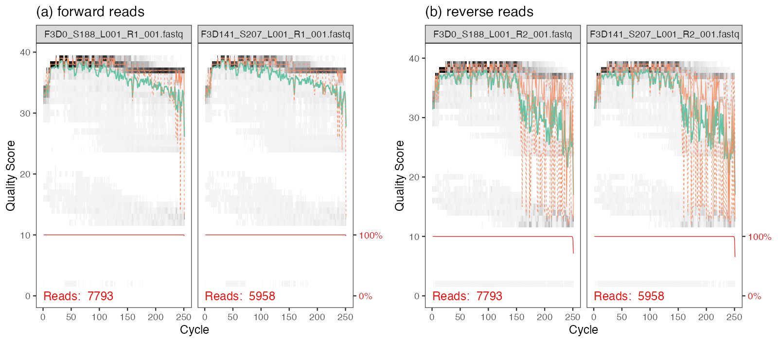
Figure 5.39. Quality profiles of the first two samples, (a) forward and (b) reverse reads (7,793 and 5,958 reads). Code: fig_5_39. Reproduces Holmes and Huber (2019), Figure 5.39. PDFExercise 5.6. Make the same plots for four randomly chosen samples and compare forward and reverse reads.
Solution
ii <- sample(length(fnFs), 4), thenplotQualityProfile(fnFs[ii])andplotQualityProfile(fnRs[ii]). In every sample the forward reads keep a median quality near 35 to about position 240, while the reverse reads deteriorate steadily and fall sharply after about position 160, the usual pattern of Illumina paired-end runs (the reverse read is sequenced later, after more cycles of chemistry). This motivates the truncation lengths of Exercise 5.7.Exercise 5.7. Filter and trim the read pairs: truncate forward reads at 240 and reverse reads at 160, remove the first 10 bases, discard reads with ambiguous bases and reads with more than 2 expected errors, filtering pairs jointly.
Solution
\[ \mathrm{EE}=\E\Big[\sum_s\ind[\text{error at }s]\Big]=\sum_s10^{-Q_s/10}, \]filterAndTrim(fnFs, filtFs, fnRs, filtRs, truncLen = c(240, 160), trimLeft = 10, maxN = 0, maxEE = 2, truncQ = 2, rm.phix = TRUE). Paired filtering (both files given at once) drops a pair if either read fails, which keeps the files in step for merging. The expected number of errors of a read is a direct consequence of the meaning of quality scores: a Phred score \(Q_s\) at position \(s\) means an error probability \(e_s=10^{-Q_s/10}\), and by linearity of expectation the expected number of errors iswhatever the dependence between positions. A read of 230 bases all at \(Q=30\) has \(\mathrm{EE}=0.23\); a single base at \(Q=2\) contributes 0.63. Filtering on EE is better than filtering on the average quality, because the average of \(Q\) hides a few very bad bases (EE is dominated by the lowest scores). The book's output shows that about 90% of the reads pass (e.g. 7,793 to 7,139 for the first sample).
Exercise 5.8. Make a map like Figure 5.2: download addresses of bomb impacts, geocode them and plot them on a map of London.
Solution
Method: obtain the list of impact addresses (or coordinates) from the archive, convert addresses into latitude and longitude with a geocoding service, check failures and duplicates, and plot the points over map tiles (for instance with ggplot2 and a tile provider, or leaflet). To test whether the impacts are "clustered" beyond chance, compare the point pattern with complete spatial randomness (Chapter 11 of the book: Ripley's K function or quadrat counts against a Poisson process with the same intensity); the historical analysis of such data found a good fit to a Poisson distribution of hits per area (Clarke 1946).
Demonstrations for this chapter
Each demonstration runs in the browser on the data of the chapter (exported by the R code), with seeded random numbers, and links back to these notes. The ▶ Demo boxes above open them set to the case under discussion. Their computations agree with R: see the last column.
| Demonstration | What you can see | Agreement with R |
|---|---|---|
| k-means, k-medoids and PAM, step by step | Assign and update steps with the objective after each, the decomposition \(J=\WSS+\sum n_m|\bar x_m-c_m|^2\), local minima, BUILD and SWAP, Euclidean and Manhattan medoids. Presets: 1 poor start (Fig. 5.12); 2 a local minimum; 3 alternating k-medoids stuck; 4 PAM; 5 PAM, Manhattan; 6 spirals (Fig. 5.38a); 7 uniform data. | Final WSS 2903.7853 from the same start as kmeans(algorithm = "Lloyd"); PAM medoids and objectives (3.10390, 2.41338) identical to cluster::pam. |
| How many clusters? gap, Calinski-Harabasz and silhouettes | PAM for \(k=1,\dots,K\), \(\log W_k\) against uniform references, the gap with \(\pm s_k\) and three rules, CH, average silhouette and the silhouette plot. Presets: 1 four groups; 2 uniform; 3, 4 embryo cells (Fig. 5.31); 5 squared distances; 6 silhouettes. | \(\log W_k\), CH and average silhouettes equal to clusGap, calinhara and silhouette to all printed digits; Monte Carlo gap within 0.005 of clusGap. |
| Hierarchical clustering: linkages, dendrograms and cuts | Trees built merge by merge with five linkages, cuts into \(k\) clusters, chaining, inversions, cophenetic correlation, T-cell heatmaps. Presets 1 to 8. | Merge heights equal to hclust for all five linkages; cophenetic correlation 0.8425 (average linkage, T cells) as in R. |
| Mass cytometry: the asinh transform and DBSCAN | Histograms before and after asinh, DBSCAN with core, border and noise points, the k-distance plot, the spirals. Presets 1 to 6. | Cluster sizes, core and noise counts equal to dbscan::dbscan on the same 5,000 cells (e.g. 3,845 core, 721 noise, clusters 4,089, 183, 7). |
The R code that produces every figure of this page is code/ch05_clustering.R (see the code index).
References
- Holmes, S. and Huber, W. (2019). Modern Statistics for Modern Biology. Cambridge University Press, Cambridge. Chapter 5.
- Bendall, S. C., Simonds, E. F., Qiu, P., et al. (2011). Single-cell mass cytometry of differential immune and drug responses across a human hematopoietic continuum. Science, 332(6030), 687–696. doi:10.1126/science.1198704.
- Callahan, B. J., McMurdie, P. J., Rosen, M. J., Han, A. W., Johnson, A. J. A. and Holmes, S. P. (2016). DADA2: high-resolution sample inference from Illumina amplicon data. Nature Methods, 13(7), 581–583. doi:10.1038/nmeth.3869.
- Callahan, B. J., McMurdie, P. J. and Holmes, S. P. (2017). Exact sequence variants should replace operational taxonomic units in marker-gene data analysis. The ISME Journal, 11, 2639–2643. doi:10.1038/ismej.2017.119.
- Caliński, T. and Harabasz, J. (1974). A dendrite method for cluster analysis. Communications in Statistics, 3(1), 1–27. doi:10.1080/03610927408827101.
- Clarke, R. D. (1946). An application of the Poisson distribution. Journal of the Institute of Actuaries, 72(3), 481.
- Ester, M., Kriegel, H.-P., Sander, J. and Xu, X. (1996). A density-based algorithm for discovering clusters in large spatial databases with noise. In Proceedings of the Second International Conference on Knowledge Discovery and Data Mining (KDD-96), 226–231. AAAI Press.
- Hornik, K. (2005). A CLUE for CLUster Ensembles. Journal of Statistical Software, 14(12). doi:10.18637/jss.v014.i12.
- Kaufman, L. and Rousseeuw, P. J. (2009). Finding Groups in Data: An Introduction to Cluster Analysis. Wiley, Hoboken, NJ.
- Lance, G. N. and Williams, W. T. (1967). A general theory of classificatory sorting strategies: 1. Hierarchical systems. The Computer Journal, 9(4), 373–380. doi:10.1093/comjnl/9.4.373.
- Le Cam, L. (1960). An approximation theorem for the Poisson binomial distribution. Pacific Journal of Mathematics, 10(4), 1181–1197. doi:10.2140/pjm.1960.10.1181.
- Müllner, D. (2013). fastcluster: fast hierarchical, agglomerative clustering routines for R and Python. Journal of Statistical Software, 53(9), 1–18. doi:10.18637/jss.v053.i09.
- Ohnishi, Y., Huber, W., Tsumura, A., et al. (2014). Cell-to-cell expression variability followed by signal reinforcement progressively segregates early mouse lineages. Nature Cell Biology, 16(1), 27–37. doi:10.1038/ncb2881.
- Rosen, M. J., Callahan, B. J., Fisher, D. S. and Holmes, S. P. (2012). Denoising PCR-amplified metagenome data. BMC Bioinformatics, 13, 283. doi:10.1186/1471-2105-13-283.
- Rousseeuw, P. J. (1987). Silhouettes: a graphical aid to the interpretation and validation of cluster analysis. Journal of Computational and Applied Mathematics, 20, 53–65. doi:10.1016/0377-0427(87)90125-7.
- Schubert, E. and Rousseeuw, P. J. (2019). Faster k-medoids clustering: improving the PAM, CLARA, and CLARANS algorithms. In Similarity Search and Applications (SISAP 2019), Lecture Notes in Computer Science 11807, 171–187. Springer.
- Schwarz, G. (1978). Estimating the dimension of a model. The Annals of Statistics, 6(2), 461–464. doi:10.1214/aos/1176344136.
- Tibshirani, R., Walther, G. and Hastie, T. (2001). Estimating the number of clusters in a data set via the gap statistic. Journal of the Royal Statistical Society: Series B, 63(2), 411–423. doi:10.1111/1467-9868.00293.
- Tseng, G. C. and Wong, W. H. (2005). Tight clustering: a resampling-based approach for identifying stable and tight patterns in data. Biometrics, 61(1), 10–16. doi:10.1111/j.0006-341X.2005.031032.x.
- Tversky, A. and Kahneman, D. (1974). Judgment under uncertainty: heuristics and biases. Science, 185(4157), 1124–1131. doi:10.1126/science.185.4157.1124.
The numerical statements in the text (book outputs reproduced, the PAM and k-means values, the DBSCAN tables, the Lance-Williams heights, the CH erratum, the gap computations, the Le Cam bound, the boundary shift and the model-based clustering) are computed by the course code.