Survival Analysis and Censored Data
Some responses are times: time until death, until a paper is published, until a call is answered. Their difficulty is not the shape of their distribution but that many of them are only partly seen: a patient alive at the end of the study has a survival time that is at least the follow-up time. This chapter shows how to use such censored observations instead of throwing them away. The Kaplan–Meier estimator builds the survival curve one death at a time, the log-rank test compares curves one death at a time, and Cox's proportional hazards model relates survival to predictors through a partial likelihood that never needs the baseline hazard. The same sequential idea gives the lasso for survival data, the concordance index and survival trees. Every figure is recomputed here.
Ch. 1 Introduction Ch. 2 Statistical learning Ch. 3 Linear regression Ch. 4 Classification Ch. 5 Resampling Ch. 6 Selection and regularization Ch. 7 Beyond linearity Ch. 8 Trees Ch. 9 SVMs Ch. 10 Deep learning Ch. 11 Survival analysis Ch. 12 Unsupervised learning Ch. 13 Multiple testing
How to read these notes
They follow the book. Sections carry the book's numbers (11.3, 11.5.2, ...), and displayed equations that appear in the book carry its equation numbers, e.g. \((11.16)\); equations without a number are steps the book skips. Page numbers refer to the R edition (2021); the Python edition (2023) has the same text, figures and exercises a few pages later.
Filling the gaps. Where the book says that a result "can be shown", states it without proof or skips steps, an orange Filling the gap box gives the complete argument at the level of a first course in statistics. Derivations start hidden: open one with its bar, or use the button below. Green Deeper lines point to the graduate course on the same authors' larger book.
The lab in two languages. Section 11.8 shows each step in R (left) and Python (right), with the output and the figures. The R code uses the survival package. The Python code uses numpy, pandas, scipy and statsmodels only: the Kaplan–Meier estimator and the log-rank test are written out as short functions, and Cox's model is fitted with statsmodels' PHReg. Both give the same numbers.
Main reference
G. James, D. Witten, T. Hastie and R. Tibshirani, An Introduction to Statistical Learning with Applications in R, 2nd edition, Springer (2021), Chapter 11, pages 461–495, and G. James, D. Witten, T. Hastie, R. Tibshirani and J. Taylor, An Introduction to Statistical Learning with Applications in Python, Springer (2023), Chapter 11 (book website, with the data and the labs: www.statlearning.com). Section, equation, figure and exercise numbers below refer to these books.
The explanations, derivations, figures and code are my own; equations are cited by their numbers in the book.
Companion courses
- Statistical Learning: Theory and Methods (Hastie, Tibshirani and Friedman 2009): survival analysis appears in Section 18.6 (supervised principal components for survival data), with a compact account of Kaplan–Meier, the log-rank test and the Cox score in Filling the gap 18.6; the lasso in Section 3.4.2; trees in Section 9.2.
- Statistical Methods for Modern Biology (Holmes and Huber 2019): the hypergeometric distribution behind the log-rank test, and the AUC as a probability, which the C-index generalises.
- Earlier chapters of this course: logistic regression and Newton's method (Algorithm 4.1), the ROC curve (Figure 4.8), cross-validation and the bootstrap (Section 5.1.3, Definition 5.5) and the lasso (Section 6.2.2).
The chapter at a glance
- 11.1–11.2 We observe \(y_i=\min(t_i,c_i)\) and whether it is a death. Everything that follows assumes independent censoring: given the predictors, the censoring time carries no information about the survival time, so the patients still under observation at any time are a fair sample of those still alive (Filling the gap 11.1).
- 11.3 The Kaplan–Meier estimator multiplies, over the death times, the estimated probabilities of surviving each one given survival so far (Result 11.1). It is the nonparametric maximum likelihood estimator (Filling the gap 11.3), and its variance is given by Greenwood's formula (Filling the gap 11.4).
- 11.4 The log-rank test adds up, over the death times, the deaths observed in one group minus those expected if both groups had the same hazard. Each term is centred hypergeometric (Result 11.2), and the terms are uncorrelated, so the variances add (Filling the gap 11.7).
- 11.5 The hazard \(h(t)=f(t)/S(t)\) and \(S(t)=\exp(-\int_0^th)\) are equivalent descriptions of a survival distribution (Result 11.3). Cox's model \(h(t\given x)=h_0(t)e^{x^\T\beta}\) is fitted by the partial likelihood (11.16), in which \(h_0\) cancels (Filling the gap 11.10); it is concave, Newton's method fits it (Algorithm 11.1), and its score test for one binary predictor is the log-rank test (Result 11.7).
- 11.6–11.7 The lasso penalises the negative log partial likelihood; models are compared by a cross-validated partial likelihood deviance, the concordance index and the time-dependent AUC, which handle censoring by using only the pairs whose order is known.
Notation. Patient \(i\) has survival time \(t_i\), censoring time \(c_i\), observed time \(y_i=\min(t_i,c_i)\) and status \(\delta_i=1\) for a death, 0 for a censored time; \(x_i\in\R^p\) are its predictors. \(d_1\lt d_2\lt\dots\lt d_K\) are the distinct death times, \(q_k\) the number of deaths at \(d_k\), and \(r_k\) the number at risk just before \(d_k\) (observed time \(\ge d_k\)); \(\Rk_k\) is that risk set. In two groups, \(r_{1k},q_{1k}\) and \(r_{2k},q_{2k}\) are the same counts within each group.
Prerequisites. Conditional probability and the law of total probability, maximum likelihood with its score, information and the delta method, logistic regression (Chapter 4), cross-validation and the bootstrap (Chapter 5) and the lasso (Chapter 6).
pp. 461–462 In a five-year cancer study, a patient still alive after five years has a survival time we do not know, except that it exceeds five years. Dropping such patients would discard the best-surviving part of the sample and bias every estimate downwards; treating five years as their survival time would bias it too. The same structure appears far from medicine: the time until a customer cancels a subscription (customers who have not cancelled yet are censored), or a weight measured on a scale that cannot show values above its maximum (heavy people are censored at that maximum). Survival analysis is the set of methods that use the partial information in censored values correctly.
11.1 Survival and Censoring Times
Definition 11.1 (survival time, censoring time, observed time, status) p. 462, (11.1)
Each individual has a survival time \(T\) (also called failure time or event time: the time of death, relapse, cancellation, ...) and a censoring time \(C\) (the time at which observation stops: the end of the study, drop-out). We observe only
\[ Y=\min(T,C) \tag{11.1} \]and the status indicator \(\delta=1\) if \(T\le C\) (the event was seen, \(Y=T\)), \(\delta=0\) if \(T>C\) (censored, \(Y=C\), and all we know is \(T>Y\)). The data are \(n\) pairs \((y_1,\delta_1),\dots,(y_n,\delta_n)\), usually with predictors \(x_1,\dots,x_n\).
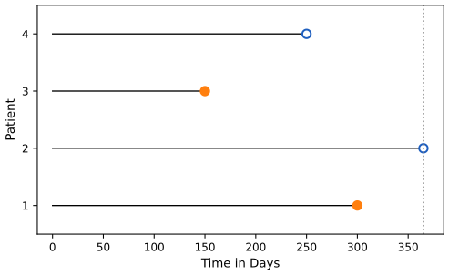
fig_11_1. Reproduces James et al. (2021), Figure 11.1. Download: PDF · SVG11.2 A Closer Look at Censoring
p. 463 Whether censored data can be analysed at all depends on why the censoring happened. If the sickest patients leave a cancer study early, those remaining look healthier than the population, and an analysis that ignores the reason will overestimate survival. If very sick men leave more often than very sick women, a comparison of the sexes will flatter the men.
Definition 11.2 (independent censoring; right, left and interval censoring) pp. 463–464
The censoring mechanism is independent if, conditional on the predictors, the survival time \(T\) and the censoring time \(C\) are independent. This cannot be checked from the data: it is an assumption about how the data were collected. The chapter assumes it throughout.
The censoring above is right censoring: the true time is at least the observed one, \(T\ge Y\). In left censoring the true time is at most the observed one (pregnancies already ended when women are surveyed 250 days after conception); in interval censoring it is only known to lie in an interval (a weekly check that the event has happened). Both can be handled with variants of the methods below; the chapter treats right censoring only.
Filling the gap 11.1: what independent censoring buys, and the "non-informative" condition of the footnote p. 463 and footnote 1
Derivation
The risk set is a fair sample. Every method in the chapter estimates, at each time \(t\), the chance of dying soon among those "at risk": still observed, \(Y\ge t\), which means \(T\ge t\) and \(C\ge t\). What we want is the chance among those still alive, \(T\ge t\). If \(T\) and \(C\) are independent, then for a small \(\Delta\)
\[ \Pr(t\le T\lt t+\Delta\given T\ge t,\ C\ge t)=\frac{\Pr(t\le T\lt t+\Delta,\ C\ge t)}{\Pr(T\ge t,\ C\ge t)}=\frac{\Pr(t\le T\lt t+\Delta)\Pr(C\ge t)}{\Pr(T\ge t)\Pr(C\ge t)}=\Pr(t\le T\lt t+\Delta\given T\ge t). \]The factor \(\Pr(C\ge t)\) cancels: being still under observation tells us nothing about the risk of dying next. If instead sick patients leave early, \(\Pr(C\ge t\given T)\) is larger for long-lived patients, the factor no longer cancels, and the observed death rate among those at risk is too low.
Non-informative censoring. The book's footnote mentions a weaker condition. Write the likelihood of one observation when \(T\) has density \(f\) and survival function \(S\), and \(C\) has density \(g\) and survival function \(G\), independently. A death at \(y\) means \(T=y\) and \(C\ge y\): contribution \(f(y)G(y)\). A censoring at \(y\) means \(C=y\) and \(T\gt y\): contribution \(g(y)S(y)\). So
\[ L_i=\big[f(y_i)^{\delta_i}S(y_i)^{1-\delta_i}\big]\times\big[g(y_i)^{1-\delta_i}G(y_i)^{\delta_i}\big]. \]If the parameters of \(g,G\) have nothing to do with those of \(f,S\) (censoring is non-informative), the second bracket is a constant as far as the survival parameters are concerned and can be dropped. What remains is the likelihood (11.12) of Section 11.5.1. All the methods of the chapter (Kaplan–Meier, the log-rank test, Cox's partial likelihood) can be derived from it.
11.3 The Kaplan–Meier Survival Curve
Definition 11.3 (survival function) p. 464, (11.2)
\[ S(t)=\Pr(T\gt t). \tag{11.2} \]It starts at \(S(0)=1\) and decreases. For a subscription service with \(T\) the time of cancellation, \(S(t)\) is the probability that a customer is still subscribed at time \(t\).
pp. 464–465 The BrainCancer data (Selingerová et al. 2016) follow 88 patients with primary brain tumours treated with stereotactic radiation. The predictors are the gross tumour volume gtv (cm3), sex, diagnosis (meningioma, low-grade glioma, high-grade glioma, other), the tumour location loc (infratentorial or supratentorial), the Karnofsky index ki (a 0–100 score of how well the patient can carry out ordinary activities) and the method stereo (radiosurgery SRS or fractionated radiotherapy SRT). There are 35 deaths; the other 53 times are censored.
How should we estimate \(S(20)\), the probability of living more than 20 months? Two naive answers:
- the share of all patients with \(y_i\gt20\): \(48/88=0.545\). This counts the 17 patients censored before 20 months as if they had died before 20 months;
- the share among the patients not censored before 20 months: \(48/71=0.676\). This throws the 17 away, although a patient censored at 19.9 months almost certainly lived past 20.
The Kaplan–Meier estimate is 0.713, higher than both (Filling the gap 11.5 explains why).
Result 11.1 (the Kaplan–Meier estimator) pp. 465–466, (11.3)
With distinct death times \(d_1\lt\dots\lt d_K\), \(q_k\) deaths at \(d_k\) and \(r_k\) patients at risk just before \(d_k\),
\[ \hat S(d_k)=\prod_{j=1}^k\frac{r_j-q_j}{r_j}, \tag{11.3} \]and \(\hat S(t)=\hat S(d_k)\) for \(d_k\le t\lt d_{k+1}\) (\(\hat S(t)=1\) before \(d_1\)): a step function that drops only at death times. Censored patients count in the risk sets up to their censoring time and then leave them; they cause no drop.
Filling the gap 11.2: the product of conditional probabilities, step by step p. 465
Derivation
The chain. Since \(T\gt d_k\) implies \(T\gt d_{k-1}\), the event \(\{T\gt d_k\}\) equals \(\{T\gt d_k\}\cap\{T\gt d_{k-1}\}\), so by the definition of conditional probability (the book uses the law of total probability, whose second term is zero)
\[ S(d_k)=\Pr(T\gt d_k\given T\gt d_{k-1})\,S(d_{k-1})=\dots=\prod_{j=1}^k\Pr(T\gt d_j\given T\gt d_{j-1}),\qquad d_0=0. \]Each factor. No death is observed strictly between \(d_{j-1}\) and \(d_j\), so the natural estimate puts no probability of dying there: \(\Pr(T\gt d_j\given T\gt d_{j-1})\) is estimated by the probability of surviving the death time \(d_j\) itself, given being alive just before it. Just before \(d_j\), \(r_j\) patients are alive and observed, and by Filling the gap 11.1 they are a fair sample of those alive; \(q_j\) of them die at \(d_j\). The proportion surviving, \((r_j-q_j)/r_j\), estimates the factor, which gives (11.3).
Where censored patients go. A patient censored at \(c\) with \(d_{j-1}\le c\lt d_j\) belongs to the risk sets \(r_1,\dots,r_{j-1}\) and not to \(r_j,\dots\): their information (alive at \(c\)) is used exactly as long as it is valid. A censoring time equal to a death time is counted as at risk at that death time (the convention of R's survfit: the patient is assumed to have outlived the deaths recorded at the same time).
Two checks. Without censoring, \(r_{j+1}=r_j-q_j\), the product telescopes to \(r_{k+1}/n\), and \(\hat S(t)\) is the share of patients with \(y_i\gt t\): the empirical survival function. On the brain cancer data the first death is at 0.07 months with 88 at risk (\(\hat S=87/88=0.9886\)); the next time, 1.18, is a censoring (no drop, the risk set falls to 86); the death at 1.41 gives \(0.9886\times85/86=0.9771\).
Filling the gap 11.3: Kaplan–Meier is the nonparametric maximum likelihood estimator p. 466
Derivation
Allow any distribution for \(T\), but note that the likelihood (11.12) can only be large if the distribution puts probability on the observed death times (a continuous density would make every \(f(y_i)\) zero relative to a point mass). So consider distributions that put probability only at \(d_1,\dots,d_K\) (and possibly beyond the last time), and describe them by their discrete hazards \(\lambda_k=\Pr(T=d_k\given T\ge d_k)\). Then \(\Pr(T\gt t)=\prod_{d_k\le t}(1-\lambda_k)\) and \(\Pr(T=d_k)=\lambda_k\prod_{j\lt k}(1-\lambda_j)\).
A patient who dies at \(d_k\) contributes \(\lambda_k\prod_{j\lt k}(1-\lambda_j)\); a patient censored at \(c\) contributes \(S(c)=\prod_{d_j\le c}(1-\lambda_j)\). Collect, for each \(k\), the factors involving \(\lambda_k\): every one of the \(r_k\) patients at risk at \(d_k\) contributes either \(\lambda_k\) (the \(q_k\) who die there) or \(1-\lambda_k\) (the \(r_k-q_k\) who survive it, whether they die or are censored later). So
\[ L(\lambda_1,\dots,\lambda_K)=\prod_{k=1}^K\lambda_k^{q_k}(1-\lambda_k)^{r_k-q_k}. \]This is a product of binomial likelihoods, one per death time, each in its own parameter. Each is maximised at \(\hat\lambda_k=q_k/r_k\) (set the derivative of \(q_k\log\lambda_k+(r_k-q_k)\log(1-\lambda_k)\) to zero), and therefore
\[ \hat S(t)=\prod_{d_k\le t}(1-\hat\lambda_k)=\prod_{d_k\le t}\frac{r_k-q_k}{r_k}, \]which is (11.3): the Kaplan–Meier curve is the maximum likelihood estimate among all distributions (Kaplan and Meier 1958). The same factorisation reappears in the log-rank test (each \(d_k\) gives a 2×2 table) and in Cox's partial likelihood (each \(d_k\) gives one factor).
Filling the gap 11.4: Greenwood's formula and the band of Figure 11.2 p. 466 and Exercise 10
Derivation
Take logarithms: \(\log\hat S(t)=\sum_{d_k\le t}\log(1-\hat\lambda_k)\). Treat the \(\hat\lambda_k=q_k/r_k\) as independent binomial proportions (they are asymptotically uncorrelated, for the reason given in Filling the gap 11.7), with \(\Var\hat\lambda_k\approx\hat\lambda_k(1-\hat\lambda_k)/r_k\). The delta method with \(\frac{d}{d\lambda}\log(1-\lambda)=-1/(1-\lambda)\) gives
\[ \Var\log(1-\hat\lambda_k)\approx\frac{\hat\lambda_k(1-\hat\lambda_k)}{r_k(1-\hat\lambda_k)^2}=\frac{q_k}{r_k(r_k-q_k)},\qquad\widehat\Var\log\hat S(t)=\sum_{d_k\le t}\frac{q_k}{r_k(r_k-q_k)}. \]A second application of the delta method (\(\hat S=e^{\log\hat S}\)) gives Greenwood's formula \(\widehat\Var\hat S(t)=\hat S(t)^2\sum_{d_k\le t}q_k/[r_k(r_k-q_k)]\).
The band. R's survfit() reports \(\mathrm{se}=\sqrt{\sum q_k/[r_k(r_k-q_k)]}\), the standard error of \(\log\hat S(t)\), and its default 95% interval is \(\hat S(t)\exp(\pm1.96\,\mathrm{se})\), built on the log scale and cut at 1. This is the dashed band of Figure 11.2 (the caption calls it a standard error band). At 20 months: \(\hat S=0.713\), standard error of \(\hat S\) 0.051, interval \((0.620,\,0.820)\). The band widens with time because the risk sets shrink (48 patients at 20 months, 5 at 60).
Median survival. The estimated median is the first time with \(\hat S(t)\le0.5\): 47.8 months; the curve ends at 0.452 after the last death at 51 months, with only censored times after it.
Filling the gap 11.5: why Kaplan–Meier beats both naive estimates: redistribution to the right pp. 464–466
Derivation
Kaplan–Meier can be computed by an equivalent recipe (Efron 1967). Give each of the \(n\) observations mass \(1/n\). Go through the times in increasing order; when you reach a censored time, give its mass away, in equal shares, to all the observations with a larger time. At the end the mass sits on the death times (and on the largest times if they are censored), and \(\hat S(t)\) is the mass beyond \(t\).
Why it is the same. Suppose that just before \(d_k\) the \(r_k\) observations at risk all carry the same mass \(m\), so that \(\hat S(d_k^-)=r_km\). The \(q_k\) deaths keep their mass, so \(\hat S\) drops to \((r_k-q_k)m=\hat S(d_k^-)(r_k-q_k)/r_k\), the Kaplan–Meier factor. A censoring among the survivors spreads its mass equally on those with larger times, which keeps all their masses equal (each grows by the same factor), and keeps \(\hat S\) unchanged.
The two naive estimates. 48/88 leaves each early-censored patient's mass where it is, below 20 months, as if they had died. 48/71 removes those 17 masses and rescales the rest equally, as if each censored patient's future were that of a random patient, including those who had already died before the censoring. Kaplan–Meier sends each censored mass only to the patients known to be alive later. So it puts more mass beyond 20 months than either: 0.713 against 0.676 and 0.545.
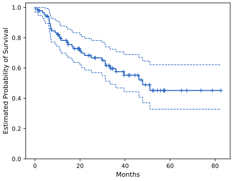
fig_11_2, km_table in ch11_lab.py. Reproduces James et al. (2021), Figure 11.2. Download: PDF · SVGDeeper: Statistical Learning: Theory and Methods, Filling the gap 18.6 (Kaplan–Meier, Greenwood, the log-rank test and the Cox score in a high-dimensional application).
p. 466 The sequential construction, which follows the events as they happen in time, is the key idea of the whole chapter: the log-rank test and Cox's model are built in the same way.
11.4 The Log-Rank Test
pp. 466–467 Do men and women with brain tumours survive equally long? Figure 11.3 suggests that women do a little better for about 50 months. A two-sample \(t\)-test on the observed times would be wrong: it compares the \(y_i\), not the \(t_i\), and censoring shortens the \(y_i\) differently in the two groups. The log-rank test instead compares the groups at each death time.
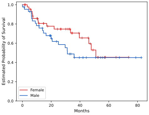
fig_11_3. Reproduces James et al. (2021), Figure 11.3. Download: PDF · SVGAt each death time \(d_k\) the patients at risk form a 2×2 table (the book's Table 11.1):
| Group 1 | Group 2 | Total | |
|---|---|---|---|
| Died | \(q_{1k}\) | \(q_{2k}\) | \(q_k\) |
| Survived | \(r_{1k}-q_{1k}\) | \(r_{2k}-q_{2k}\) | \(r_k-q_k\) |
| Total | \(r_{1k}\) | \(r_{2k}\) | \(r_k\) |
To test \(H_0:\E X=0\) for a random variable \(X\), a natural statistic is
\[ W=\frac{X-\E(X)}{\sqrt{\Var(X)}}, \tag{11.4} \]with the mean and variance computed under \(H_0\). The log-rank test takes \(X=\sum_kq_{1k}\), the total number of deaths in group 1. Under the null hypothesis of equal survival, and conditioning on the margins of each table,
\[ \E(q_{1k})=\frac{r_{1k}}{r_k}q_k, \tag{11.5} \] \[ \Var(q_{1k})=\frac{q_k(r_{1k}/r_k)(1-r_{1k}/r_k)(r_k-q_k)}{r_k-1}, \tag{11.6} \] \[ \Var\Big(\sum_{k=1}^Kq_{1k}\Big)\approx\sum_{k=1}^K\Var(q_{1k})=\sum_{k=1}^K\frac{q_k(r_{1k}/r_k)(1-r_{1k}/r_k)(r_k-q_k)}{r_k-1}, \tag{11.7} \] \[ W=\frac{\sum_{k=1}^K\big(q_{1k}-\E(q_{1k})\big)}{\sqrt{\sum_{k=1}^K\Var(q_{1k})}}=\frac{\sum_{k=1}^K\big(q_{1k}-\frac{q_k}{r_k}r_{1k}\big)}{\sqrt{\sum_{k=1}^K\frac{q_k(r_{1k}/r_k)(1-r_{1k}/r_k)(r_k-q_k)}{r_k-1}}}. \tag{11.8} \]For large samples \(W\) is approximately \(\N(0,1)\) under \(H_0\); equivalently \(W^2\) is approximately \(\chi^2_1\), the form R's survdiff() prints.
Result 11.2 (the null distribution of each table) p. 468, (11.5)–(11.6); Exercise 7
If the two groups have the same hazard, then, given the margins \(r_{1k},r_k,q_k\) of the table at \(d_k\), the number of deaths in group 1 is hypergeometric: it is distributed as the number of group-1 patients among \(q_k\) drawn without replacement from the \(r_k\) at risk, of whom \(r_{1k}\) are in group 1,
\[ \Pr(q_{1k}=a)=\binom{r_{1k}}{a}\binom{r_k-r_{1k}}{q_k-a}\Big/\binom{r_k}{q_k}, \]with mean (11.5) and variance (11.6).
Filling the gap 11.6: why the table is hypergeometric, and its mean and variance p. 468, footnote 5; Exercise 7
Derivation
Why hypergeometric. Under \(H_0\) all patients at risk at \(d_k\) have the same chance of dying there, whatever their group. Given that exactly \(q_k\) of the \(r_k\) die, every set of \(q_k\) patients is equally likely to be the one that dies (by symmetry). Counting the sets with \(a\) members from group 1 (choose them among \(r_{1k}\)) and \(q_k-a\) from group 2 (among \(r_k-r_{1k}\)) gives the formula of Result 11.2: a hypergeometric distribution with population \(r_k\), \(r_{1k}\) "successes" and \(q_k\) draws.
Mean. Number the \(r_{1k}\) group-1 patients and let \(I_j=1\) if patient \(j\) is among the \(q_k\) who die. Each patient is equally likely to be in the death set, so \(\E I_j=q_k/r_k\), and \(\E q_{1k}=\sum_jE I_j=r_{1k}q_k/r_k\), which is (11.5).
Variance. \(\Var I_j=\frac{q_k}{r_k}(1-\frac{q_k}{r_k})\), and for two different patients \(\Pr(I_j=I_l=1)=\frac{q_k(q_k-1)}{r_k(r_k-1)}\), so
\[ \Cov(I_j,I_l)=\frac{q_k(q_k-1)}{r_k(r_k-1)}-\frac{q_k^2}{r_k^2}=-\frac{q_k(r_k-q_k)}{r_k^2(r_k-1)}. \]Summing \(r_{1k}\) variances and \(r_{1k}(r_{1k}-1)\) covariances,
\[ \Var q_{1k}=r_{1k}\frac{q_k(r_k-q_k)}{r_k^2}-r_{1k}(r_{1k}-1)\frac{q_k(r_k-q_k)}{r_k^2(r_k-1)}=\frac{q_k(r_k-q_k)}{r_k^2}\,r_{1k}\,\frac{r_k-r_{1k}}{r_k-1}, \]which is (11.6) written as \(q_k\frac{r_{1k}}{r_k}\big(1-\frac{r_{1k}}{r_k}\big)\frac{r_k-q_k}{r_k-1}\). The last factor is the finite-population correction: without it, this is the binomial variance of \(q_k\) draws with replacement. When deaths are untied (\(q_k=1\)) it equals 1 and \(\Var q_{1k}=p_k(1-p_k)\), \(p_k=r_{1k}/r_k\): a single Bernoulli draw.
Filling the gap 11.7: the terms are uncorrelated, so the variances add; the test for several groups; the brain cancer numbers p. 468, (11.7)
Derivation
Uncorrelated, not just "nonetheless". The book notes that \(q_{11},\dots,q_{1K}\) may be correlated and adds the variances anyway. The centred terms \(u_k=q_{1k}-\E(q_{1k})\) are in fact uncorrelated. Let \(\mathcal{F}_k\) be everything that happened up to just before \(d_k\) (who died or was censored earlier, hence the risk set), together with \(q_k\). Result 11.2 says that, given \(\mathcal{F}_k\), \(q_{1k}\) has mean \(e_k=q_kr_{1k}/r_k\), which is itself known given \(\mathcal{F}_k\). So \(\E(u_k\given\mathcal{F}_k)=0\). For \(j\lt k\), \(u_j\) is known given \(\mathcal{F}_k\), hence
\[ \E(u_ju_k)=\E\big[u_j\,\E(u_k\given\mathcal{F}_k)\big]=0. \]The \(u_k\) form a martingale difference sequence: uncorrelated, though not independent (the risk sets depend on earlier deaths). So \(\Var(\sum_ku_k)=\sum_k\E\Var(u_k\given\mathcal{F}_k)\), estimated without bias by \(\sum_k\Var(q_{1k})\) from (11.6), and the martingale central limit theorem justifies the normal approximation for \(W\). The approximation sign in (11.7) is about the variances being estimated, not about neglected correlations.
Several groups. With \(G\) groups the deaths at \(d_k\) follow a multivariate hypergeometric distribution: the group counts have means \(q_kr_{gk}/r_k\) and covariance matrix \(q_k\frac{r_k-q_k}{r_k-1}\big(\diag(\bm p_k)-\bm p_k\bm p_k^\T\big)\), \(\bm p_k=(r_{gk}/r_k)_g\). Summing gives observed counts \(\bm O\), expected counts \(\bm E\) and a covariance \(\bV\) that is singular (the counts add up to \(q_k\)); dropping one group, \((\bm O-\bm E)^\T\bV^{-1}(\bm O-\bm E)\) is approximately \(\chi^2_{G-1}\). This is what survdiff() and the lab's logrank_test compute for the call-centre data.
The numbers. Taking women as group 1: 15 observed deaths, 18.539 expected, variance 8.697, so \(W=(15-18.539)/\sqrt{8.697}=-1.200\), \(W^2=1.4405\) and two-sided \(p=0.230\) (the book's "W = 1.2" and "p-value of 0.2" are the rounded values). A permutation test (Section 13.5) that shuffles the sex labels 1000 times gives \(p=0.238\) here and 0.25 in the book; the two differ only by the random permutations.
See also: the hypergeometric distribution in Statistical Methods for Modern Biology, where it gives Fisher's exact test for enrichment.
Deeper: Statistical Learning: Theory and Methods, Filling the gap 18.6 (the log-rank statistic as a Cox score).
pp. 468–469 On the brain cancer data the log-rank test gives no evidence of a difference between the sexes. The test is closely related to Cox's model: Result 11.7 shows that it is the score test of a Cox model with the group as its only predictor.
11.5 Regression Models With a Survival Response
p. 469 With predictors \(x\in\R^p\), we would like to predict \(T\). Regressing \(\log Y\) on \(x\) by least squares fails for the same reason as before: censored \(y_i\) understate \(t_i\). The remedy is again sequential, and it goes through the hazard function.
11.5.1 The Hazard Function
Definition 11.4 (hazard function, density, cumulative hazard) pp. 469–470, (11.9)–(11.11)
\[ h(t)=\lim_{\Delta t\to0}\frac{\Pr(t\lt T\le t+\Delta t\given T\gt t)}{\Delta t}, \tag{11.9} \]the death rate just after \(t\) among those alive at \(t\) (also called the hazard rate or force of mortality). It is a rate, not a probability: \(h(t)\Delta t\) is approximately the probability of dying in a short interval \((t,t+\Delta t]\) given survival to \(t\). The density is
\[ f(t)=\lim_{\Delta t\to0}\frac{\Pr(t\lt T\le t+\Delta t)}{\Delta t}, \tag{11.11} \]and the cumulative hazard is \(H(t)=\int_0^th(u)\,du\).
Result 11.3 (three equivalent descriptions of a survival distribution) p. 470, (11.10); Exercise 8
\[ h(t)=\frac{f(t)}{S(t)}, \tag{11.10} \] \[ f(t)=\frac{dF(t)}{dt}=-\frac{dS(t)}{dt},\qquad h(t)=-\frac{d}{dt}\log S(t),\qquad S(t)=\exp\Big(-\int_0^th(u)\,du\Big)=e^{-H(t)}. \]So any one of \(f\), \(S\), \(h\) determines the other two.
Filling the gap 11.8: proof of Result 11.3, and the footnote's "density conditional on \(T\gt t\)" pp. 469–470, footnote 7; Exercise 8
Derivation
(11.10). \(\Pr(t\lt T\le t+\Delta t\given T\gt t)=\Pr(t\lt T\le t+\Delta t)/\Pr(T\gt t)\), because the event \(t\lt T\le t+\Delta t\) is contained in \(T\gt t\). Divide by \(\Delta t\) and let \(\Delta t\to0\): the numerator gives \(f(t)\) by (11.11), the denominator is \(S(t)\).
\(f=dF/dt\). \(\Pr(t\lt T\le t+\Delta t)=F(t+\Delta t)-F(t)\), with \(F(t)=1-S(t)=\Pr(T\le t)\), so (11.11) is the derivative of \(F\), i.e. \(-S'(t)\).
\(S=e^{-H}\). By the chain rule \(\frac{d}{dt}\log S(t)=S'(t)/S(t)=-f(t)/S(t)=-h(t)\). Integrate from 0 to \(t\), using \(\log S(0)=\log1=0\): \(\log S(t)=-\int_0^th(u)\,du\).
Footnote 7, made precise. The conditional distribution of \(T\) given \(T\gt t\) has density \(f(s)/S(t)\) for \(s\gt t\). Its value at the left end \(s=t\) is \(f(t)/S(t)=h(t)\). So \(h(t)\) is that conditional density evaluated at \(t\); the conditional density changes with \(t\), which is why the hazard is a function rather than one density.
Examples. The exponential distribution has constant hazard \(\lambda\), \(H(t)=\lambda t\) and \(S(t)=e^{-\lambda t}\) (Exercise 9): it has no memory, since a patient alive at \(t\) faces the same future as a new one. A Weibull hazard \(h(t)=\alpha\gamma t^{\gamma-1}\) increases (\(\gamma\gt1\)) or decreases (\(\gamma\lt1\)) with time, and \(S(t)=e^{-\alpha t^\gamma}\); Figure 11.4 below and the simulated call centre of the lab use \(\gamma=2\) and 3.
p. 470 If observation \(i\) is a death at \(y_i\), its likelihood is the density at \(y_i\); if it is censored at \(y_i\), it is the probability of surviving past \(y_i\):
\[ L_i=\begin{cases}f(y_i)&\text{if the }i\text{th observation is not censored}\\S(y_i)&\text{if the }i\text{th observation is censored}\end{cases}\;=f(y_i)^{\delta_i}S(y_i)^{1-\delta_i}, \tag{11.12} \] \[ L=\prod_{i=1}^nf(y_i)^{\delta_i}S(y_i)^{1-\delta_i}=\prod_{i=1}^nh(y_i)^{\delta_i}S(y_i), \tag{11.13} \]assuming independent observations; the second form uses \(f=hS\). Filling the gap 11.1 shows why the censoring distribution does not appear.
Result 11.4 (the exponential model) p. 471; Exercise 9
If \(T\sim\mathrm{Exp}(\lambda)\), the likelihood (11.13) is \(\prod_i\lambda^{\delta_i}e^{-\lambda y_i}=\lambda^{D}e^{-\lambda\sum_iy_i}\) with \(D=\sum_i\delta_i\) the number of deaths, and
\[ \hat\lambda=\frac{\sum_{i=1}^n\delta_i}{\sum_{i=1}^ny_i}=\frac{\text{deaths}}{\text{total time at risk}},\qquad\widehat{\E T}=\frac1{\hat\lambda}=\frac{\sum_iy_i}{\sum_i\delta_i}. \]On the brain cancer data: 35 deaths in 2416.3 patient-months, \(\hat\lambda=0.0145\) per month, an estimated mean survival of 69.0 months, and \(\hat S(20)=e^{-20\hat\lambda}=0.748\), against 0.713 from Kaplan–Meier (the constant hazard does not fit the higher death rate of the first months).
Exercise 9 asks for the derivation: \(\log L=D\log\lambda-\lambda\sum y_i\) has derivative \(D/\lambda-\sum y_i\), zero at \(\hat\lambda\), and second derivative \(-D/\lambda^2\lt0\). Note that dividing the total observed time by the number of deaths, not by \(n\), is what corrects for censoring: the censored patients contribute time at risk but no death.
p. 471 Richer parametric families (gamma, Weibull) are fitted in the same way. To bring in predictors, it is convenient to model the hazard: for example \(h(t\given x_i)=\exp(\beta_0+\sum_j\beta_jx_{ij})\), an exponential model whose rate depends on \(x_i\). That assumes a hazard constant in time, which is restrictive. Cox's model keeps the dependence on \(x\) and lets the time dependence be anything.
11.5.2 Proportional Hazards
Definition 11.5 (the proportional hazards assumption) p. 471, (11.14)
\[ h(t\given x_i)=h_0(t)\exp\Big(\sum_{j=1}^px_{ij}\beta_j\Big), \tag{11.14} \]with \(h_0(t)\ge0\) an unspecified baseline hazard (the hazard of an individual with all predictors 0). The factor \(\exp(\sum_jx_{ij}\beta_j)\) is the relative risk of \(x_i\) against \(x=0\). Increasing \(x_{ij}\) by one unit multiplies the hazard at every time by \(e^{\beta_j}\), whatever the other predictors and whatever \(t\). There is no intercept: it would be absorbed into \(h_0\).
Result 11.5 (what proportional hazards implies for the survival curves) p. 472, Figure 11.4
Under (11.14), \(S(t\given x)=S_0(t)^{\exp(x^\T\beta)}\) with \(S_0=e^{-H_0}\) the baseline survival function, and \(\log(-\log S(t\given x))=\log H_0(t)+x^\T\beta\). Hence the log hazards of two individuals differ by a constant, their survival curves never cross, and their curves of \(\log(-\log S)\) against time are parallel.
Filling the gap 11.9: proof of Result 11.5 p. 472
Derivation
By Result 11.3, \(S(t\given x)=\exp\big(-\int_0^th_0(u)e^{x^\T\beta}du\big)=\exp\big(-e^{x^\T\beta}H_0(t)\big)=\big(e^{-H_0(t)}\big)^{e^{x^\T\beta}}\). Taking \(-\log\) and then \(\log\) gives \(\log(-\log S(t\given x))=\log H_0(t)+x^\T\beta\). For two individuals the difference \((x-x')^\T\beta\) does not depend on \(t\); in particular, if \(x^\T\beta\gt x'^\T\beta\) then \(S(t\given x)\lt S(t\given x')\) at every \(t\gt0\) with \(0\lt S_0(t)\lt1\) (a number in \((0,1)\) raised to a larger power is smaller), so the curves cannot cross. The gap between the curves starts at zero and widens at first, as the book observes; it shrinks again only when both curves approach 0. Crossing survival curves, as in the bottom row of Figure 11.4, are therefore evidence against (11.14); this is the basis of the graphical check of Section 11.7.4.
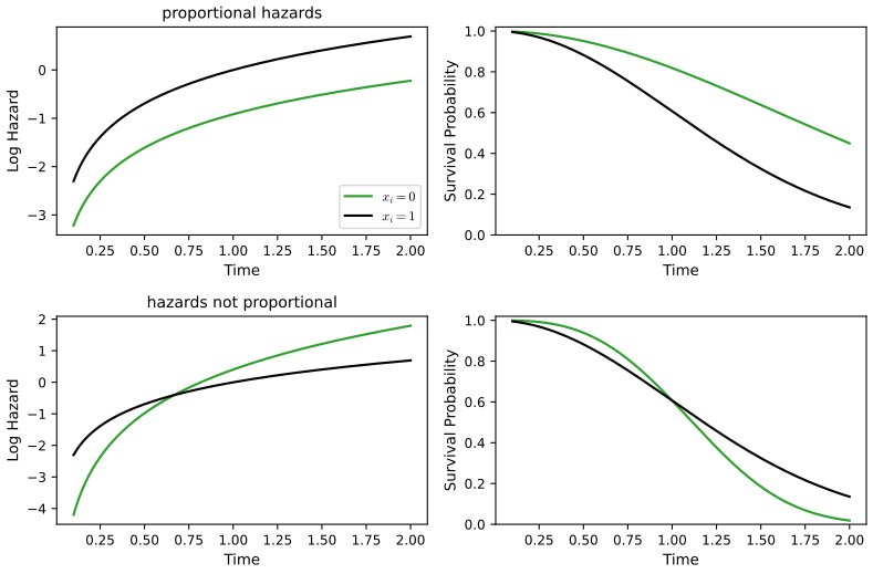
fig_11_4. Reproduces James et al. (2021), Figure 11.4. Download: PDF · SVGCox's proportional hazards model
p. 473 Because \(h_0\) is unknown, (11.14) cannot be put into the likelihood (11.13). Cox's idea is to look at the deaths one at a time. Assume for now that no two deaths happen at the same time, and let patient \(i\) die at \(y_i\). The total hazard of the patients at risk at that moment is \(\sum_{i':y_{i'}\ge y_i}h_0(y_i)\exp(\sum_jx_{i'j}\beta_j)\), and the probability that the death is that of patient \(i\), rather than of another patient at risk, is
\[ \frac{h_0(y_i)\exp\big(\sum_{j=1}^px_{ij}\beta_j\big)}{\sum_{i':y_{i'}\ge y_i}h_0(y_i)\exp\big(\sum_{j=1}^px_{i'j}\beta_j\big)}=\frac{\exp\big(\sum_{j=1}^px_{ij}\beta_j\big)}{\sum_{i':y_{i'}\ge y_i}\exp\big(\sum_{j=1}^px_{i'j}\beta_j\big)}. \tag{11.15} \]The baseline hazard cancels. The partial likelihood is the product of these probabilities over the deaths:
\[ \PL(\beta)=\prod_{i:\delta_i=1}\frac{\exp\big(\sum_{j=1}^px_{ij}\beta_j\big)}{\sum_{i':y_{i'}\ge y_i}\exp\big(\sum_{j=1}^px_{i'j}\beta_j\big)}. \tag{11.16} \]It is valid whatever \(h_0\) is, and \(\hat\beta\) maximises it. As for logistic regression there is no closed form; Newton's method is used (Algorithm 11.1), and the usual standard errors, confidence intervals and tests follow from the curvature of \(\log\PL\) at its maximum.
Filling the gap 11.10: where (11.15) comes from, and why (11.16) is a "partial" likelihood p. 473, footnote 13 and p. 474
Derivation
(11.15) as a limit. Let \(\Rk(y_i)=\{i':y_{i'}\ge y_i\}\) be the risk set. In a short interval \([y_i,y_i+\Delta)\), patient \(i'\) dies with probability \(h(y_i\given x_{i'})\Delta+o(\Delta)\), independently of the others. The probability that exactly one dies and that it is \(i\) is \(h(y_i\given x_i)\Delta\prod_{i'\ne i}(1-h(y_i\given x_{i'})\Delta)+o(\Delta)\), and the probability that exactly one dies, whoever it is, is \(\sum_{i'\in\Rk}h(y_i\given x_{i'})\Delta\prod_{i''\ne i'}(\dots)+o(\Delta)\). Their ratio tends, as \(\Delta\to0\), to \(h(y_i\given x_i)/\sum_{i'\in\Rk}h(y_i\given x_{i'})\), and with (11.14) the common factor \(h_0(y_i)\) cancels. The same form is the probability that the first of several independent exponential clocks with rates \(\lambda_{i'}\) to ring is clock \(i\): \(\lambda_i/\sum\lambda_{i'}\).
Why "partial". The full likelihood (11.13) of \((y_i,\delta_i)\) can be written as the product of two parts: the probabilities (11.15) of who dies at each death time given that someone does, and the probabilities of the death times and censorings themselves. Only the first part is free of \(h_0\). Cox (1972, 1975) proposed to maximise it alone; it is not the probability of the data, but it behaves like a likelihood: its score has mean zero, its curvature estimates the variance of \(\hat\beta\), and \(\hat\beta\) is consistent and asymptotically normal. Filling the gap 11.13 gives a second justification: maximising the full likelihood over \(h_0\) first and then over \(\beta\) gives the same \(\hat\beta\).
Result 11.6 (score and information of the partial likelihood) p. 473
Let \(w_{i'}=e^{x_{i'}^\T\beta}\) and, for the death of patient \(i\), let \(\bar x_i(\beta)=\sum_{i'\in\Rk(y_i)}w_{i'}x_{i'}/\sum_{i'\in\Rk(y_i)}w_{i'}\) be the weighted mean of the predictors over the risk set and \(\bV_i(\beta)\) their weighted covariance matrix. Then
\[ \ell(\beta)=\log\PL(\beta)=\sum_{i:\delta_i=1}\Big[x_i^\T\beta-\log\sum_{i'\in\Rk(y_i)}e^{x_{i'}^\T\beta}\Big],\qquad U(\beta)=\nabla\ell=\sum_{i:\delta_i=1}\big(x_i-\bar x_i(\beta)\big),\qquad I(\beta)=-\nabla^2\ell=\sum_{i:\delta_i=1}\bV_i(\beta). \]\(I(\beta)\) is a sum of covariance matrices, so it is positive semi-definite: \(\ell\) is concave, and any maximum is global (unique when \(I\) is positive definite).
Filling the gap 11.11: the derivatives, and the score as observed minus expected p. 473
Derivation
Write \(S_0=\sum_{\Rk}w_{i'}\), \(S_1=\sum_{\Rk}w_{i'}x_{i'}\), \(S_2=\sum_{\Rk}w_{i'}x_{i'}x_{i'}^\T\). Since \(\nabla w_{i'}=w_{i'}x_{i'}\), we have \(\nabla S_0=S_1\) and \(\nabla S_1=S_2\). So \(\nabla\log S_0=S_1/S_0=\bar x\), and
\[ \nabla^2\log S_0=\frac{S_2}{S_0}-\frac{S_1S_1^\T}{S_0^2}=\sum_{\Rk}\pi_{i'}x_{i'}x_{i'}^\T-\bar x\bar x^\T=\bV,\qquad\pi_{i'}=\frac{w_{i'}}{S_0}. \]The \(\pi_{i'}\) are the probabilities (11.15), so \(\bar x\) and \(\bV\) are the mean and covariance of the predictors of the patient who dies, as the model predicts it. Summing over deaths gives Result 11.6. The score therefore reads "observed minus expected": the predictors of the patients who actually died, minus the predictors expected for them by the model, death by death. At \(\hat\beta\) the two balance.
Brain cancer, sex only. With \(x=1\) for men, \(U(0)=3.539\) and \(I(0)=8.697\). Newton's method from 0 gives 0.40698, then 0.407669, then 0.4076685 (converged); \(\hat\beta=0.4077\) with standard error \(1/\sqrt{I(\hat\beta)}=0.342\).
Algorithm 11.1 (Newton's method for Cox's model) p. 473
- Start at \(\beta^{(0)}=0\).
- Repeat: compute \(U(\beta^{(m)})\) and \(I(\beta^{(m)})\) by one pass over the death times (the risk sets are nested, so the sums \(S_0,S_1,S_2\) can be accumulated from the longest time backwards); set \(\beta^{(m+1)}=\beta^{(m)}+I(\beta^{(m)})^{-1}U(\beta^{(m)})\), halving the step if \(\ell\) does not increase.
- Stop when the change in \(\ell\) is negligible. The estimated covariance of \(\hat\beta\) is \(I(\hat\beta)^{-1}\).
The Python lab fits with statsmodels' PHReg, R with coxph(); both are this algorithm (the Python lab first takes a few quasi-Newton steps, which cannot overshoot when a predictor has large outliers).
Connection with the log-rank test
p. 474 To compare two groups we can either fit a Cox model with the group indicator as its only predictor and test \(H_0:\beta=0\), or run a log-rank test. Of the usual tests of \(H_0\) in Cox's model (likelihood ratio, Wald, score), the score test is the log-rank test.
Result 11.7 (the score test is the log-rank test) p. 474
For one binary predictor \(x_i\in\{0,1\}\) and no tied death times, the score statistic \(U(0)^2/I(0)\) of \(H_0:\beta=0\) in Cox's model equals the squared log-rank statistic \(W^2\) of (11.8), with group 1 the patients with \(x=1\). With tied deaths, the equality holds for the exact partial likelihood of discrete times (R's ties = "exact"), and only approximately for the Breslow and Efron approximations.
Filling the gap 11.12: proof of Result 11.7, the three tests, and what ties change p. 474
Derivation
Proof. At \(\beta=0\) all weights are 1, so for a death at \(d_k\) the weighted mean of a binary \(x\) over the risk set is the share \(p_k=r_{1k}/r_k\) of group 1 among those at risk, and the weighted variance is \(p_k(1-p_k)\). By Result 11.6, with one death at each \(d_k\),
\[ U(0)=\sum_k\big(q_{1k}-p_k\big)=\sum_k\Big(q_{1k}-\frac{q_kr_{1k}}{r_k}\Big),\qquad I(0)=\sum_kp_k(1-p_k), \]which are the numerator of (11.8) and its variance (11.6) with \(q_k=1\) (then \((r_k-q_k)/(r_k-1)=1\)). Hence \(U(0)/\sqrt{I(0)}=W\). On the brain cancer data (men as group 1): \(U(0)=20-16.461=3.539\), \(I(0)=8.697\), and \(U^2/I=1.44050\), exactly the survdiff chi-squared.
The three tests. Likelihood ratio: \(2[\ell(\hat\beta)-\ell(0)]\); Wald: \(\hat\beta^\T I(\hat\beta)\hat\beta\) (here \((\hat\beta/\mathrm{se})^2\)); score: \(U(0)^\T I(0)^{-1}U(0)\). All are approximately \(\chi^2_p\) under \(H_0\), and close to each other when the log partial likelihood is close to a quadratic, as here: 1.4388, 1.4209 and 1.4405 for sex. The score test needs no fit at all, which is why the log-rank test is so cheap.
Ties. With \(q_k\) deaths at \(d_k\), (11.16) has to be modified. Breslow's approximation treats them as if they happened one after the other in the full risk set: factor \(\prod_{i\in D_k}w_i/S_0^{q_k}\). Efron's approximation (R's default) removes the dying patients gradually: \(\prod_{i\in D_k}w_i\big/\prod_{l=0}^{q_k-1}\big(S_0-\tfrac{l}{q_k}\sum_{D_k}w_i\big)\). The exact version takes the probability that the death set is \(D_k\) among all sets of \(q_k\) at risk, which at \(\beta=0\) is the hypergeometric model of Result 11.2. Its score test is therefore the log-rank test, while Breslow's information at 0 is \(\sum_kq_kp_k(1-p_k)\), without the factor \((r_k-q_k)/(r_k-1)\). On the Publication data (156 publications, 22 of them at a time shared with another): log-rank 0.8440 (= exact), Breslow 0.8430, Efron 0.8409. The differences are negligible, but the book's "exactly equal" needs untied times.
Additional details
pp. 474–475 Four points the book only mentions: there is no intercept (absorbed into \(h_0\)); tied death times need an approximation (Filling the gap 11.12); (11.16) is not the probability of the data (Filling the gap 11.10); and estimating \(S(t\given x)\) needs an estimate of \(h_0\), which the book leaves to R. Here it is.
Filling the gap 11.13: the Breslow estimator of the baseline hazard, and the partial likelihood as a profile likelihood pp. 474–475
Derivation
As in Filling the gap 11.3, let the baseline put hazard only at the death times: increments \(\eta_k\ge0\) at \(d_k\), so that \(H_0(t)=\sum_{d_k\le t}\eta_k\). Treating time as continuous with these jumps, the full log-likelihood (11.13) of the Cox model is (no ties)
\[ \log L(\beta,\eta)=\sum_k\Big[\log\eta_k+x_{(k)}^\T\beta\Big]-\sum_{i=1}^ne^{x_i^\T\beta}H_0(y_i)=\sum_k\Big[\log\eta_k+x_{(k)}^\T\beta-\eta_k\sum_{i\in\Rk_k}e^{x_i^\T\beta}\Big], \]with \(x_{(k)}\) the predictors of the patient who dies at \(d_k\), since \(H_0(y_i)=\sum_{k:d_k\le y_i}\eta_k\) and \(d_k\le y_i\) means \(i\in\Rk_k\). For fixed \(\beta\), each \(\eta_k\) is maximised at
\[ \hat\eta_k(\beta)=\frac{q_k}{\sum_{i\in\Rk_k}e^{x_i^\T\beta}}\qquad(\text{the Breslow estimator, here with }q_k=1). \]Substituting back, \(\log L(\beta,\hat\eta(\beta))=\sum_k\big[x_{(k)}^\T\beta-\log\sum_{\Rk_k}e^{x_i^\T\beta}\big]-K=\log\PL(\beta)-K\). So the partial likelihood is the full likelihood with \(h_0\) profiled out: maximising one or the other gives the same \(\hat\beta\) (Johansen 1983). The estimated survival curve of an individual with predictors \(x\) is then \(\hat S(t\given x)=\exp\big(-\hat H_0(t)e^{x^\T\hat\beta}\big)\), \(\hat H_0(t)=\sum_{d_k\le t}\hat\eta_k(\hat\beta)\). With no predictors it is close to Kaplan–Meier (it is the exponential of minus the Nelson–Aalen estimator). With ties and Efron's method, R's survfit() uses the increment \(\sum_{l=0}^{q_k-1}1/\big(S_0-\tfrac{l}{q_k}\sum_{D_k}w_i\big)\); the lab's cox_survival implements both versions and reproduces R's curves to \(10^{-9}\).
11.5.3 Example: Brain Cancer Data
p. 475 Table 11.2 is the Cox model with all six predictors (87 patients: one has no diagnosis). Here it is, recomputed (R's coxph and the Python lab agree to all digits shown).
| coefficient | std. error | z | p-value | hazard ratio | |
|---|---|---|---|---|---|
| sex[Male] | 0.184 | 0.360 | 0.51 | 0.61 | 1.20 |
| diagnosis[LG glioma] | 0.915 | 0.638 | 1.43 | 0.15 | 2.50 |
| diagnosis[HG glioma] | 2.155 | 0.451 | 4.78 | 1.7e-6 | 8.62 |
| diagnosis[Other] | 0.886 | 0.658 | 1.35 | 0.18 | 2.42 |
| loc[Supratentorial] | 0.441 | 0.704 | 0.63 | 0.53 | 1.55 |
| ki | −0.055 | 0.018 | −3.00 | 0.0027 | 0.95 |
| gtv | 0.034 | 0.022 | 1.54 | 0.12 | 1.03 |
| stereo[SRT] | 0.178 | 0.602 | 0.30 | 0.77 | 1.19 |
Baselines: female, meningioma, infratentorial, SRS. Likelihood ratio test of all eight coefficients: 41.4 on 8 df, \(p=1.8\times10^{-6}\). Reading the table: with the other predictors fixed, the estimated hazard of a man is \(e^{0.184}=1.20\) times that of a woman at every time (not significant, \(p=0.61\)); a high-grade glioma multiplies the hazard by \(e^{2.155}=8.62\) relative to a meningioma; each extra point of the Karnofsky index multiplies it by \(e^{-0.055}=0.946\), so 10 points by 0.58. The book phrases the hazard ratio as a "greater chance of dying"; strictly it is a ratio of instantaneous death rates, which translates into a ratio of probabilities only over short intervals.
11.5.4 Example: Publication Data
pp. 475–476 The Publication data (Gordon et al. 2013) record, for 244 clinical trials funded by the National Heart, Lung, and Blood Institute, the time in months from the end of the trial to the publication of its results; 156 were published during follow-up and 88 are censored. The predictors are whether the trial had a clinical endpoint (clinend), was multi-centre (multi), the funding mechanism (mech, 14 levels), the sample size, the budget, a citation-based impact score and whether the result was positive (posres).
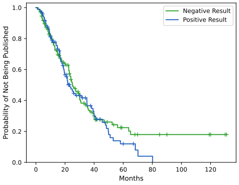
fig_11_5. Reproduces James et al. (2021), Figure 11.5. Download: PDF · SVGPositive trials seem to be published a little sooner, but the log-rank test gives \(p=0.36\). With all predictors in a Cox model (Table 11.3) the picture changes: posres has coefficient 0.552 (standard error 0.183, \(p=0.003\)), so a positive trial is published at \(e^{0.552}=1.74\) times the rate of a negative one with the same other characteristics. The adjustment matters because positive and negative trials differ in other respects: only 7 of the 98 positive trials had a clinical endpoint, against 38 of the 146 negative ones, and trials with a clinical endpoint are published much faster. Adjusting for clinend alone already gives posres a coefficient of 0.561 (\(p=0.002\)): the crude comparison mixes the faster publication of positive results with the slower publication of the trials that tend to produce them. clinend (0.511, \(p=0.06\)) and impact (0.060 per point, \(z=8.2\)) are the other strong effects; the funding mechanism adds little.
Filling the gap 11.14: the two coefficients of Table 11.3 near −15 have no estimate p. 477, Table 11.3
Derivation
Table 11.3 reports \(-14.78\) (standard error 3414) for mech[R42] and \(-14.92\) (2244) for mech[RC2]. Each of these mechanisms funded a single trial, and neither was published. A patient who never dies appears in the denominators of (11.16) but in no numerator; if their indicator has its own coefficient \(\beta_m\), letting \(\beta_m\to-\infty\) removes their term \(e^{x^\T\beta}\) from every denominator and so increases every factor. The partial likelihood keeps increasing, and the maximum is at \(-\infty\) (a monotone likelihood, the survival analogue of separation in logistic regression). R stops when the increase becomes negligible, around \(-15\), and warns that the coefficients "may be infinite"; the huge standard errors are a symptom, not an estimate. In the limit the two trials drop out of every risk set, so the other coefficients converge to those of the model fitted without these two trials. That limit is what the Python lab computes; it agrees with R's other 17 coefficients to \(10^{-9}\), as does the maximised log partial likelihood.
p. 477 Figure 11.6 shows the adjusted survival curves: the Cox model's \(\hat S(t\given x)\) for a positive and a negative trial, with every other predictor at its mean and mech at its most common level, R01. They separate clearly: 24 months after the end of the trial, 57.5% of such negative trials are unpublished against 38.3% of positive ones.
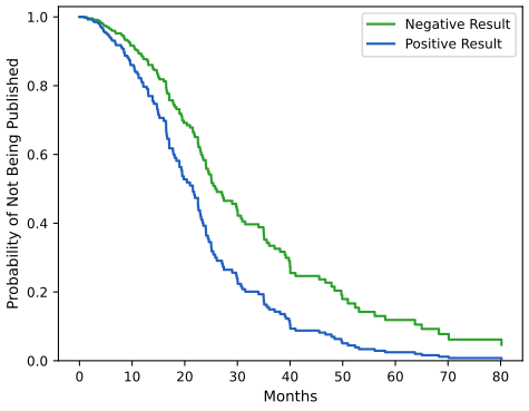
mech = R01; \(\hat H_0\) is the Efron-corrected Breslow estimator (Filling the gap 11.13). Code: fig_11_6, cox_survival. Reproduces James et al. (2021), Figure 11.6. Download: PDF · SVGA caution about impact, the strongest predictor: it is a citation-based measure of the publication, and it is 0 for 87 of the 88 unpublished trials (and for 10 of the 156 published ones). It is therefore largely a consequence of the outcome rather than a characteristic of the trial known at time zero (Notes on the book). The adjusted effect of posres does not depend on it: without impact (and mech) its coefficient is 0.536, \(p=0.003\).
11.6 Shrinkage for the Cox Model
p. 478 The "loss + penalty" idea of Section 6.2 carries over with the negative log partial likelihood as the loss:
\[ -\log\Bigg(\prod_{i:\delta_i=1}\frac{\exp\big(\sum_{j=1}^px_{ij}\beta_j\big)}{\sum_{i':y_{i'}\ge y_i}\exp\big(\sum_{j=1}^px_{i'j}\beta_j\big)}\Bigg)+\lambda P(\beta), \tag{11.17} \]with \(P(\beta)=\sum_j\beta_j^2\) (ridge) or \(P(\beta)=\sum_j|\beta_j|\) (lasso) and \(\lambda\ge0\) a tuning parameter. \(\lambda=0\) gives Cox's estimate; as \(\lambda\) grows the coefficients shrink, and with the lasso some become exactly 0.
Filling the gap 11.15: how the lasso Cox model is fitted, and the largest useful \(\lambda\) p. 478
Derivation
Scaling. R's glmnet (used for the book's Figure 11.7) minimises \(-\frac1n\ell(\beta)+\lambda\sum_j|\beta_j|\) on standardised predictors (mean 0, standard deviation 1 with divisor \(n\)), with Breslow's handling of ties; this is (11.17) with \(\lambda\) multiplied by \(n\). The code here (cox_lasso) minimises the same function and reproduces glmnet's coefficients to \(10^{-6}\) on the Publication data.
Proximal Newton. At the current \(\beta\), replace \(-\frac1n\ell\) by its second-order Taylor expansion, which uses the score and information of Result 11.6. The resulting problem, a quadratic plus \(\lambda\|\beta\|_1\), is a lasso least-squares problem, solved by cycling through the coordinates: for coordinate \(j\), with \(H\) the Hessian and \(g\) the gradient of the quadratic at the current point, the minimiser is the soft-thresholded Newton update
\[ \beta_j\leftarrow\frac{\mathcal S\big(H_{jj}\beta_j-g_j,\ \lambda\big)}{H_{jj}},\qquad\mathcal S(z,\lambda)=\sign(z)\max(|z|-\lambda,0). \]A line search on the penalised objective keeps each outer step a descent step; glmnet uses the same scheme with a diagonal approximation to the Hessian.
The largest useful \(\lambda\). \(\beta=0\) is optimal when 0 is in the subgradient at 0: \(\big|\frac1nU_j(0)\big|\le\lambda\) for every \(j\), with \(U(0)\) the score at 0, which by Result 11.7 is a log-rank-type "observed minus expected" sum. So the path starts at \(\lambda_{\max}=\max_j|U_j(0)|/n\), where the predictor with the largest standardised score enters first.
Monotone likelihood again. As \(\lambda\to0\), coefficients of predictors such as rarely used funding mechanisms whose trials were never published drift towards \(-\infty\) (Filling the gap 11.14): the lasso path keeps them finite for every \(\lambda\gt0\), but the unpenalised fit does not exist.
Filling the gap 11.16: cross-validation for the Cox model p. 479, footnote 15
Derivation
For least squares the cross-validation error is a sum over held-out observations. The log partial likelihood is not: each factor involves a whole risk set, and a held-out fold of 12 trials has risk sets too small to give a useful partial likelihood on its own. The standard remedy (Verweij and van Houwelingen 1993), used by glmnet and here, fits \(\hat\beta_{-k}\) without fold \(k\) and measures its fit to the fold by
where \(\ell\) uses all the training data and \(\ell_{-k}\) all but fold \(k\): the difference is the contribution of fold \(k\)'s patients, with the risk sets formed from everybody. The partial likelihood deviance plotted in Figure 11.7 is \(\sum_kD_k/(\text{number of deaths})\), computed for each \(\lambda\) on a common grid; smaller is better. The current cv.glmnet computes the same fold fits and the same \(D_k\), but measures them from the saturated model (which adds a constant that does not depend on \(\lambda\)) and divides by the number of observations rather than deaths; this moves and rescales the curve without moving its minimum. The per-death scale is the one of the book's figure (values around 9).
pp. 478–480 Following the book, the 244 trials are split at random into 122 training and 122 test trials (the book's split is not given, so ours differs). Ten-fold cross-validation of the lasso on the training set, with all 19 columns of the model matrix, gives Figure 11.7: the deviance is smallest at \(\lambda=0.147\), where two predictors are non-zero, clinend (0.514) and impact (0.038 per point). The book's split selected budget and impact. With 72 publications in the training half, the selected set depends on the split: in ten random splits impact always has the largest standardised score at \(\beta=0\), so it always enters the path first, but the variables that join it vary.
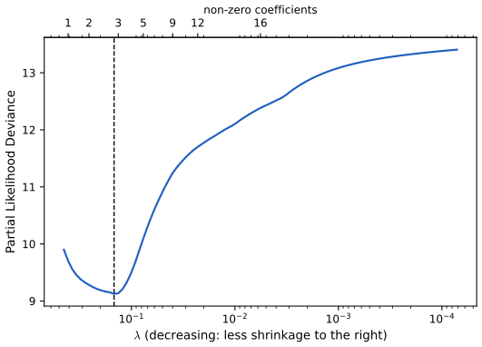
fig_11_7, lasso_path, cv_cox_lasso. Reproduces James et al. (2021), Figure 11.7. Download: PDF · SVGpp. 479–480 How good is the model on the test set? There is no simple way to compare predicted and true survival times: some test times are censored, and the Cox model predicts a whole curve \(S(t\given x)\), not a single time. Instead, each test trial gets the risk score \(\hat\eta=x^\T\hat\beta\) from the training coefficients, and the test trials are split into thirds of low, medium and high risk. A high risk score means a high hazard of publication, hence publication sooner. Figure 11.8 shows the three Kaplan–Meier curves: well separated and in the right order (log-rank \(\chi^2=83.0\) on 2 df).
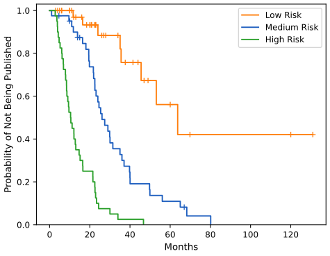
fig_11_8, tertiles. Reproduces James et al. (2021), Figure 11.8. Download: PDF · SVGDeeper: Statistical Learning: Theory and Methods, Section 3.4.2 (the lasso and soft thresholding) and Section 18.6 (survival prediction with thousands of genes). In this course: Section 6.2.2.
11.7 Additional Topics
11.7.1 Area Under the Curve for Survival Analysis
pp. 480–481 For a two-class classifier, the AUC equals the proportion of (class 1, class 2) pairs in which the class-1 observation has the higher score. For survival data, the natural analogue compares pairs of patients: the one with the higher risk score \(\hat\eta_i=\hat\beta_1x_{i1}+\dots+\hat\beta_px_{ip}\) should die first. With censoring we only know the order of \(t_i\) and \(t_{i'}\) when the shorter of the two observed times is a death. Harrell's concordance index uses exactly those pairs:
\[ C=\frac{\sum_{i,i':y_i\gt y_{i'}}I(\hat\eta_{i'}\gt\hat\eta_i)\,\delta_{i'}}{\sum_{i,i':y_i\gt y_{i'}}\delta_{i'}}. \]\(C=0.5\) is no better than chance, \(C=1\) a perfect ordering. The book's lasso model reached \(C=0.733\) on its test set; our split gives \(C=0.801\) for the lasso model and 0.789 for the unpenalised Cox model without mech, both fitted on the training half.
Filling the gap 11.17: the C-index as an AUC, ties, and the time-dependent ROC curve pp. 480–481
Derivation
As an AUC. Without censoring, and with a binary outcome "died before \(\tau\)" for a fixed \(\tau\), restricting the pairs to (died before \(\tau\), alive at \(\tau\)) turns \(C\) into the Mann–Whitney form of the AUC of Chapter 4. Harrell's \(C\) pools all such comparisons over all times. In practice ties in the score count \(\frac12\) (as in the AUC), and a censored time equal to a death time is treated as later than it; with these conventions the lab's concordance reproduces R's value 0.5647 for the model with sex only (many tied scores: every pair of the same sex is a tie).
Time-dependent AUC. Fixing a horizon \(t\), call a patient a case if they die by \(t\) and a control if they survive past \(t\); the cumulative/dynamic AUC is \(\mathrm{AUC}(t)=\Pr(\hat\eta_i\gt\hat\eta_j\given T_i\le t\lt T_j)\) (Heagerty et al. 2000). A patient censored before \(t\) is neither, and simply dropping them biases the estimate because long-lived patients are censored more often. The inverse-probability-of-censoring estimator (Uno et al. 2007) weights each case \(i\) by \(1/\hat G(y_i^-)\), with \(\hat G\) the Kaplan–Meier curve of the censoring times, the probability of still being observed at \(y_i\):
\[ \widehat{\mathrm{AUC}}(t)=\frac{\sum_i\sum_j\delta_iI(y_i\le t)I(y_j\gt t)I(\hat\eta_i\gt\hat\eta_j)/\hat G(y_i^-)}{\sum_i\sum_j\delta_iI(y_i\le t)I(y_j\gt t)/\hat G(y_i^-)}. \]On the test trials the lasso score has \(\mathrm{AUC}(12)=0.878\), \(\mathrm{AUC}(24)=0.870\) and \(\mathrm{AUC}(36)=0.804\): the score separates the trials published within about two years from the others best; beyond 50 months few controls remain and the curve is noisy (figure below).
A caution. These high values owe much to impact, which is 0 for almost every unpublished trial: it measures the outcome rather than predicting it (Notes on the book).
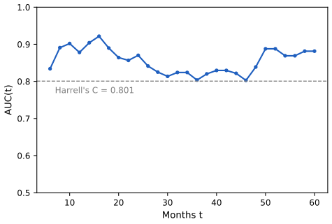
fig_auc, auc_t. Download: PDF · SVGSee also: the ROC curve of the Default data in Figure 4.8, and the AUC as a probability in Statistical Methods for Modern Biology.
11.7.2 Choice of Time Scale
p. 481 Time zero must be chosen. For the Publication data it is the end of the trial; for disease-free survival it is the date of treatment. In an epidemiological study of risk factors one may use age as the time scale (time zero at birth): the effect of age then cannot be estimated, but neither does it need to be adjusted for, since every risk set compares people of the same age. With age as time scale, people enter the study at different ages and are at risk only from their entry (delayed entry or left truncation); risk sets then contain only those already under observation.
11.7.3 Time-Dependent Covariates
pp. 481–482 Because (11.16) is built one death time at a time, a predictor whose value changes over time is easy to include: in the factor for the death at \(y_i\), use every patient's current value \(x_{i'j}(y_i)\). In the Stanford heart transplant study, coding "ever received a transplant" as a fixed predictor would credit the transplant with the survival that patients needed in order to receive one (a patient who died on the waiting list could never be coded as transplanted). This is immortal time bias. The fix is the time-dependent indicator \(x_i(t)=1\) if the transplant has happened by time \(t\): a transplanted patient counts as untransplanted in the risk sets before the transplant. In R this is done by splitting each patient's follow-up into intervals, Surv(start, stop, event).
11.7.4 Checking the Proportional Hazards Assumption
p. 482 For a qualitative predictor, plot an estimate of the log hazard, or more conveniently of the log cumulative hazard, for each level: by Result 11.5, \(\log(-\log\hat S(t))\) curves should be parallel. Quantitative predictors can be cut into strata first.
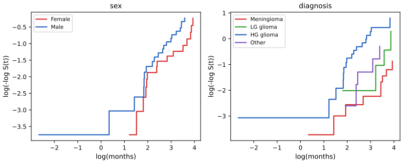
cox.zph(), finds no evidence against the assumption for the model of Table 11.2 (global \(p=0.89\)). Code: fig_loglog. Download: PDF · SVGWhen the assumption fails for one factor, a stratified Cox model gives each level its own baseline hazard while sharing the other coefficients: this is how Exercise 10(d) adjusts survival curves for the Karnofsky index (strata(ki) in R, strata= in PHReg).
11.7.5 Survival Trees
p. 482 Trees, random forests and boosting (Chapter 8) extend to survival data. A survival tree chooses each split to make the survival curves of the two daughter nodes as different as possible, usually by maximising the log-rank statistic over all predictors and cut points. On the brain cancer data the best single split of the tumour volume is \(\texttt{gtv}\le10.8\) (log-rank \(\chi^2=19.3\)), much stronger than the best split of the Karnofsky index, \(\texttt{ki}\le80\) (6.95). Note that the largest of many log-rank statistics is not \(\chi^2_1\): searching over cut points inflates it, so tree splits need cross-validation or permutation, not the nominal p-value. Each leaf reports a Kaplan–Meier curve; averaging the cumulative hazards of many such trees grown on bootstrap samples gives random survival forests (Ishwaran et al. 2008).
Deeper: Statistical Learning: Theory and Methods, Section 9.2 (tree-based methods and their split criteria).
11.8 Lab: Survival Analysis
p. 483 The lab analyses the brain cancer data, the publication data and a simulated call centre. The R lab of James et al. 2021 uses the survival package (Surv, survfit, survdiff, coxph) and simulates the call centre with the coxed package; the Python lab of James et al. 2023 uses lifelines and the authors' helper package. Here the R version follows the R lab, and the Python version computes the same quantities with numpy, pandas, scipy and statsmodels only (see the boxes "The helper functions"). The complete files are code/ch11_lab.R and code/ch11_lab.py; the excerpts below are taken from them verbatim, except that lines which only record a number in cache/ are left out.
Where the two languages differ, and why
- Same numbers. Kaplan–Meier curves and their standard errors, the log-rank tests, all Cox coefficients, standard errors and tests, and the adjusted survival curves agree to \(10^{-8}\) or better. statsmodels'
PHRegis asked for Efron's handling of ties (ties="efron"), R's default; its own default is Breslow's. - Factor coding. R keeps the order of the levels stored in the data (meningioma first for
diagnosis); the Python edition's model matrix sorts them alphabetically, so its baseline is HG glioma and its diagnosis coefficients are those of R minus 2.155 (for example \(0.915-2.155=-1.240\) for LG glioma): the same model, coded differently. The Python lab here uses R's levels. - The Wald test. R's
summary()of a Cox fit rounds the Wald statistic to two decimals (1.42); computed from the coefficient and its standard error it is 1.4209. - The call centre. Both labs draw the data from the same model with their own random number generators, so the data and the numbers differ between the languages. The Python lab reproduces the Python edition's data exactly (same wait times and test statistics); the R lab draws the waiting times by inversion instead of with
coxed. The two languages' methods are confirmed to agree by fitting each to the same data. - Survival curves of a Cox model. R's
survfit(fit, newdata = ...); in Python the baseline cumulative hazard is computed bycox_survival(Filling the gap 11.13).
11.8.1 Brain Cancer Data
Setup and a first look. 88 patients; status 1 is a death, 0 a censored time. Always check this coding: some data sets use the opposite convention.
R
suppressPackageStartupMessages({
  library(ISLR2)
  library(survival)
})
options(digits = 6, width = 100)

print(names(BrainCancer))
print(table(BrainCancer$sex))
print(table(BrainCancer$diagnosis))
print(table(BrainCancer$status))              # 1 = died (uncensored), 0 = censored
Python
BrainCancer = common.isl_data("BrainCancer", index_col=0)
print(list(BrainCancer.columns))
print(BrainCancer["sex"].value_counts())
print(BrainCancer["diagnosis"].value_counts())
print(BrainCancer["status"].value_counts())      # 1 = died (uncensored), 0 = censored
sex: Female 45, Male 43 diagnosis: Meningioma 42, LG glioma 9, HG glioma 22, Other 14 (one missing) status: 0 (censored) 53, 1 (died) 35
The Kaplan–Meier curve (Figure 11.2). Surv(time, status) pairs each time with its status.
R
fit.surv <- survfit(Surv(time, status) ~ 1, data = BrainCancer)
open_svg("lab-r-km")
plot(fit.surv, xlab = "Months", ylab = "Estimated Probability of Survival")
dev.off()
print(summary(fit.surv, times = c(10, 20, 40, 60)))
Python
km_all = km_table(BrainCancer["time"], BrainCancer["status"])
print(km_all.head(8).round(4))
print("S(t) at 10, 20, 40, 60 months:", km_at(km_all, [10, 20, 40, 60]).round(4))
fig, ax = figure()
step_plot(ax, km_all, common.BLUE, band=True)
ax.set(xlabel="Months", ylabel="Estimated Probability of Survival", ylim=(0, 1.02))
common.savefig(fig, 11, "lab-py-km", formats=("svg",))
time n.risk n.event survival std.err lower 95% CI upper 95% CI 10 67 15 0.821 0.0420 0.742 0.907 20 48 8 0.713 0.0509 0.620 0.820 40 23 9 0.552 0.0623 0.443 0.689 60 5 3 0.452 0.0736 0.328 0.621
The helper functions: km_table and km_at (Python)
def km_table(time, status):
    """Kaplan-Meier estimate at every distinct observed time, with the columns of R's survfit().

    surv is the product (11.3) of the conditional survival fractions (r_j - q_j) / r_j;
    se_logS is Greenwood's standard error of -log S(t), sqrt(sum q_j / (r_j (r_j - q_j)));
    se_S = S(t) * se_logS; lower and upper form R's default 95% interval, S(t) exp(-/+ 1.96 se_logS).
    """
    t, d = np.asarray(time, float), np.asarray(status, int)
    times = np.unique(t)
    n_risk = np.array([(t >= s).sum() for s in times])
    n_event = np.array([((t == s) & (d == 1)).sum() for s in times])
    n_censor = np.array([((t == s) & (d == 0)).sum() for s in times])
    surv = np.cumprod(1.0 - n_event / n_risk)
    with np.errstate(divide="ignore", invalid="ignore"):        # S(t) = 0 after a last death: se is undefined
        se_logS = np.sqrt(np.cumsum(np.where(n_event > 0, n_event / (n_risk * (n_risk - n_event)), 0.0)))
        return pd.DataFrame({"time": times, "n_risk": n_risk, "n_event": n_event, "n_censor": n_censor,
                             "surv": surv, "se_logS": se_logS, "se_S": surv * se_logS,
                             "lower": surv * np.exp(-Z95 * se_logS),
                             "upper": np.minimum(1.0, surv * np.exp(Z95 * se_logS))})


def km_at(table, t, column="surv"):
    """The Kaplan-Meier step function (right-continuous, 1 before the first time) at times t."""
    idx = np.searchsorted(table["time"].to_numpy(), np.atleast_1d(t), side="right") - 1
    vals = table[column].to_numpy()
    start = 1.0 if column in ("surv", "lower", "upper") else 0.0
    return np.where(idx >= 0, vals[np.maximum(idx, 0)], start)
By sex (Figure 11.3), and the log-rank test.
R
fit.sex <- survfit(Surv(time, status) ~ sex, data = BrainCancer)
open_svg("lab-r-km-sex")
plot(fit.sex, xlab = "Months", ylab = "Estimated Probability of Survival", col = c(2, 4))
legend("bottomleft", levels(BrainCancer$sex), col = c(2, 4), lty = 1)
dev.off()

logrank.test <- survdiff(Surv(time, status) ~ sex, data = BrainCancer)
print(logrank.test)
Python
fig, ax = figure()
by_sex = {}
for sex, colour in (("Female", common.RED), ("Male", common.BLUE)):
    by_sex[sex] = BrainCancer[BrainCancer["sex"] == sex]
    step_plot(ax, km_table(by_sex[sex]["time"], by_sex[sex]["status"]), colour, label=sex)
ax.legend(loc="lower left")
ax.set(xlabel="Months", ylabel="Estimated Probability of Survival", ylim=(0, 1.02))
common.savefig(fig, 11, "lab-py-km-sex", formats=("svg",))

lr = logrank_test(BrainCancer["time"], BrainCancer["status"], BrainCancer["sex"])
print(lr["table"].round(3))
print("Chisq = %.8f on %d df, p = %.4f" % (lr["chisq"], lr["df"], lr["p"]))
N Observed Expected (O-E)^2/E (O-E)^2/V sex=Female 45 15 18.5 0.676 1.44 sex=Male 43 20 16.5 0.761 1.44 Chisq= 1.4 on 1 degrees of freedom, p= 0.2 (Python: Chisq = 1.44049511, p = 0.2301)
The helper function: logrank_test (Python)
def logrank_test(time, status, group):
    """The log-rank test of equal survival in K groups (R's survdiff).

    At each distinct death time d_k with r_k at risk and q_k deaths, the deaths in group g have
    (conditional) mean q_k r_gk / r_k and the hypergeometric covariance
    q_k (r_k - q_k) / (r_k - 1) * (diag(p) - p p'),  p = (r_gk / r_k)_g.
    Summing over death times gives observed O, expected E and V; the statistic is
    (O - E)' V^- (O - E), chi-squared with K - 1 df (for K = 2 it is W^2 of (11.8)).
    """
    t, d, g = np.asarray(time, float), np.asarray(status, int), np.asarray(group)
    levels = np.unique(g)
    K = len(levels)
    O, E, V = np.zeros(K), np.zeros(K), np.zeros((K, K))
    for s in np.unique(t[d == 1]):
        at_risk = t >= s
        r = np.array([(at_risk & (g == lv)).sum() for lv in levels], float)
        q = np.array([((t == s) & (d == 1) & (g == lv)).sum() for lv in levels], float)
        rk, qk = r.sum(), q.sum()
        p = r / rk
        O += q
        E += qk * p
        if rk > 1:
            V += qk * (rk - qk) / (rk - 1) * (np.diag(p) - np.outer(p, p))
    chisq = float((O - E)[:-1] @ np.linalg.solve(V[:-1, :-1], (O - E)[:-1]))
    table = pd.DataFrame({"N": [(g == lv).sum() for lv in levels], "Observed": O, "Expected": E,
                          "(O-E)^2/E": (O - E) ** 2 / E, "(O-E)^2/V": (O - E) ** 2 / np.diag(V)},
                         index=[str(lv) for lv in levels])
    return {"table": table, "O": O, "E": E, "V": V, "chisq": chisq, "df": K - 1,
            "p": stats.chi2.sf(chisq, K - 1)}
Cox's model with sex only: the three tests, and the score test equal to the log-rank statistic (Result 11.7).
R
fit.cox <- coxph(Surv(time, status) ~ sex, data = BrainCancer)
print(summary(fit.cox))
tests <- c(LR = summary(fit.cox)$logtest[1], Wald = summary(fit.cox)$waldtest[1],
           score = summary(fit.cox)$sctest[1])
print(tests)
cat("log-rank chi-squared:", format(logrank.test$chisq, digits = 9), "\n")
Python
X_sex = model_matrix(BrainCancer, ["sex"])
fit_sex, res_sex = coxph(BrainCancer["time"], BrainCancer["status"], X_sex)
print(res_sex["table"].round(4))
print({k: round(v, 8) for k, v in res_sex["tests"].items()})
print("log-rank chi-squared: %.8f" % lr["chisq"])
C_sex = concordance(BrainCancer["time"], BrainCancer["status"], X_sex.to_numpy() @ fit_sex.params)
print("concordance %.4f" % C_sex)
coef exp(coef) se(coef) z Pr(>|z|) sexMale 0.408 1.503 0.342 1.19 0.23 Concordance= 0.565 LR.test Wald.test score.test (Python: LR 1.43882218, Wald 1.42086052, score 1.44049511) 1.43882 1.42000 1.44050 log-rank chi-squared: 1.44049511
The helper functions: model_matrix and coxph (Python)
def model_matrix(df, terms, levels=LEVELS):
    """Columns for the terms: numbers as they are, text as dummies for every level but the first."""
    cols = {}
    for v in terms:
        x = df[v]
        if x.dtype == object or isinstance(x.dtype, pd.CategoricalDtype):
            lv = levels.get(v, sorted(x.dropna().unique()))
            for level in lv[1:]:
                cols["%s%s" % (v, level)] = (x == level).astype(float).where(x.notna())
        else:
            cols[v] = x.astype(float)
    return pd.DataFrame(cols, index=df.index)


def coxph(time, status, X, ties="efron"):
    """Fit h(t | x) = h0(t) exp(x'beta) by maximising the partial likelihood (11.16) (statsmodels PHReg).

    The fit runs on standardised columns, BFGS steps first and then Newton's method (plain Newton steps
    from 0 can overshoot and overflow exp(x'beta) when a column such as budget has large outliers); the
    estimates and their covariance are then put back on the original scale. Returns the fit (params,
    bse, cov, llf) and a dictionary with R's summary table, the log partial likelihood at 0 and at the
    estimate, and the three tests of beta = 0: likelihood ratio, Wald and score.
    """
    X = pd.DataFrame(X)
    x, t, d = X.to_numpy(float), np.asarray(time, float), np.asarray(status, int)
    centre, scale = x.mean(0), x.std(0)
    scale = np.where(scale > 0, scale, 1.0)
    model_s = PHReg(t, (x - centre) / scale, status=d, ties=ties)
    with warnings.catch_warnings():                              # quasi-Newton steps first (they cannot
        warnings.simplefilter("ignore")                          # overshoot), then Newton's method to
        start = model_s.fit(method="bfgs", maxiter=200).params   # full precision
    fit_s = model_s.fit(start_params=start, method="newton")
    b = fit_s.params / scale
    cov = fit_s.cov_params() / np.outer(scale, scale)
    fit = SimpleNamespace(params=b, bse=np.sqrt(np.diag(cov)), cov=cov, llf=fit_s.llf)
    model = PHReg(t, x, status=d, ties=ties)                     # the tests, on the original scale
    zero = np.zeros(len(b))
    U, Info = model.score(zero), -model.hessian(zero)            # score and information at beta = 0
    tests = {"LR": 2 * (fit.llf - model.loglike(zero)),
             "Wald": float(b @ np.linalg.solve(cov, b)),
             "score": float(U @ np.linalg.solve(Info, U))}
    table = pd.DataFrame({"coef": b, "exp(coef)": np.exp(b), "se(coef)": fit.bse, "z": b / fit.bse,
                          "p": 2 * stats.norm.sf(np.abs(b / fit.bse))}, index=X.columns)
    return fit, {"table": table, "loglik": (model.loglike(zero), fit.llf), "tests": tests, "df": len(b)}
All predictors (Table 11.2). R drops the patient with a missing diagnosis automatically; in Python we drop it first.
R
fit.all <- coxph(Surv(time, status) ~ sex + diagnosis + loc + ki + gtv + stereo,
                 data = BrainCancer)
print(fit.all)
Python
cleaned = BrainCancer.dropna()                   # one patient has no diagnosis
terms = ["sex", "diagnosis", "loc", "ki", "gtv", "stereo"]
X_all = model_matrix(cleaned, terms)
fit_all, res_all = coxph(cleaned["time"], cleaned["status"], X_all)
print(res_all["table"].round(4))
print("likelihood ratio test = %.2f on %d df" % (res_all["tests"]["LR"], res_all["df"]))
coef exp(coef) se(coef) z p sexMale 0.1837 1.2017 0.3604 0.51 0.6101 diagnosisLG glioma 0.9150 2.4968 0.6382 1.43 0.1516 diagnosisHG glioma 2.1546 8.6241 0.4505 4.78 1.7e-06 diagnosisOther 0.8857 2.4247 0.6579 1.35 0.1782 locSupratentorial 0.4412 1.5546 0.7037 0.63 0.5307 ki -0.0550 0.9465 0.0183 -3.00 0.0027 gtv 0.0343 1.0349 0.0223 1.54 0.1247 stereoSRT 0.1778 1.1946 0.6016 0.30 0.7676 Likelihood ratio test=41.4 on 8 df, p=1.78e-06 n= 87, number of events= 35
Survival curves for each diagnosis, the other predictors at their means (numeric) or modal values (factors: female, supratentorial, SRT).
R
modaldata <- data.frame(
  diagnosis = levels(BrainCancer$diagnosis),
  sex = rep("Female", 4),
  loc = rep("Supratentorial", 4),
  ki = rep(mean(BrainCancer$ki), 4),
  gtv = rep(mean(BrainCancer$gtv), 4),
  stereo = rep("SRT", 4)
)
survplots <- survfit(fit.all, newdata = modaldata)
open_svg("lab-r-diagnosis")
plot(survplots, xlab = "Months", ylab = "Survival Probability", col = 2:5)
legend("bottomleft", levels(BrainCancer$diagnosis), col = 2:5, lty = 1)
dev.off()
print(summary(survplots, times = c(20, 60))$surv)
Python
# survival curves for each diagnosis, the other predictors at their mean (numeric) or modal value
modal = pd.DataFrame({"diagnosis": LEVELS["diagnosis"], "sex": "Female", "loc": "Supratentorial",
                      "ki": BrainCancer["ki"].mean(), "gtv": BrainCancer["gtv"].mean(), "stereo": "SRT"})
X_modal = model_matrix(modal, terms)
times, S_modal = cox_survival(cleaned["time"], cleaned["status"], X_all, fit_all.params, X_modal)
curves = pd.DataFrame(S_modal, index=times, columns=LEVELS["diagnosis"])
print(curves.iloc[[0, 1, 2, -2, -1]].round(3))
fig, ax = figure()
for k, colour in enumerate((common.RED, common.GREEN, common.BLUE, common.CYAN)):
    ax.step(np.r_[0.0, times], np.r_[1.0, S_modal[:, k]], where="post", color=colour, label=LEVELS["diagnosis"][k])
ax.legend(loc="lower left")
ax.set(xlabel="Months", ylabel="Survival Probability", ylim=(0, 1.02))
common.savefig(fig, 11, "lab-py-diagnosis", formats=("svg",))
Meningioma LG glioma HG glioma Other S(20) 0.892 0.752 0.374 0.759 S(60) 0.690 0.397 0.041 0.407
The helper function: cox_survival (Python)
def cox_survival(time, status, X, beta, Xnew, ties="efron"):
    """Survival curves S(t | x) = exp(-H0(t) exp(x'beta)) of a fitted Cox model, as R's survfit(fit, newdata).

    H0 is the baseline cumulative hazard: at a death time with q deaths it increases by
    q / sum_{risk set} exp(x'beta) (Breslow), or with Efron's correction for ties by
    sum_{l=0}^{q-1} 1 / (sum_{risk set} exp(x'beta) - (l / q) sum_{deaths} exp(x'beta)).
    Returns the death times and an array with one column per row of Xnew.
    """
    t, d = np.asarray(time, float), np.asarray(status, int)
    w = np.exp(np.asarray(X, float) @ beta)
    dtimes = np.unique(t[d == 1])
    inc = np.empty(len(dtimes))
    for k, s in enumerate(dtimes):
        risk, dead = w[t >= s].sum(), w[(t == s) & (d == 1)]
        q = len(dead)
        if ties == "efron":
            inc[k] = sum(1.0 / (risk - (l / q) * dead.sum()) for l in range(q))
        else:
            inc[k] = q / risk
    H0 = np.cumsum(inc)
    return dtimes, np.exp(-np.outer(H0, np.exp(np.asarray(Xnew, float) @ beta)))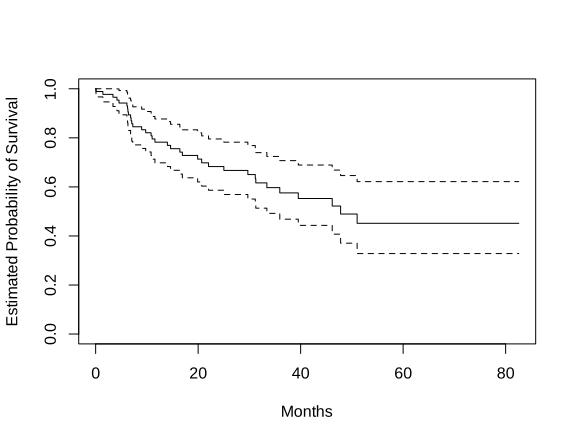
plot(fit.surv), lab-r-km.svg.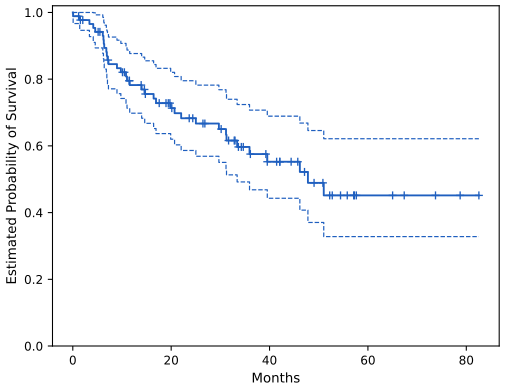
step_plot(..., band=True), lab-py-km.svg.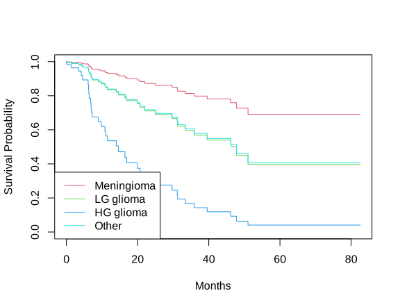
plot(survplots), lab-r-diagnosis.svg.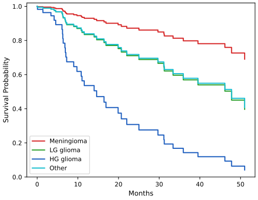
cox_survival, lab-py-diagnosis.svg.11.8.2 Publication Data
Kaplan–Meier curves by result (Figure 11.5), Cox's model with posres only and the log-rank test. Here deaths are tied (22 publications share a month value with another), so the Efron score test (0.8409) and the log-rank statistic (0.8440) differ slightly (Filling the gap 11.12).
R
fit.posres <- survfit(Surv(time, status) ~ posres, data = Publication)
open_svg("lab-r-km-posres")
plot(fit.posres, xlab = "Months", ylab = "Probability of Not Being Published", col = 3:4)
legend("topright", c("Negative Result", "Positive Result"), col = 3:4, lty = 1)
dev.off()

fit.pub <- coxph(Surv(time, status) ~ posres, data = Publication)
print(fit.pub)
logrank.test <- survdiff(Surv(time, status) ~ posres, data = Publication)
print(logrank.test)
Python
Publication = common.isl_data("Publication", index_col=0)
fig, ax = figure()
for result, colour, label in ((0, common.GREEN, "Negative Result"), (1, common.BLUE, "Positive Result")):
    part = Publication[Publication["posres"] == result]
    step_plot(ax, km_table(part["time"], part["status"]), colour, label=label)
ax.legend(loc="upper right")
ax.set(xlabel="Months", ylabel="Probability of Not Being Published", ylim=(0, 1.02))
common.savefig(fig, 11, "lab-py-km-posres", formats=("svg",))

fit_pub, res_pub = coxph(Publication["time"], Publication["status"], Publication[["posres"]])
print(res_pub["table"].round(4))
lr_pub = logrank_test(Publication["time"], Publication["status"], Publication["posres"])
print(lr_pub["table"].round(3))
print("Chisq = %.6f, p = %.4f; Cox score test = %.6f" % (lr_pub["chisq"], lr_pub["p"], res_pub["tests"]["score"]))
coef exp(coef) se(coef) z p
posres 0.148 1.160 0.162 0.92 0.36
N Observed Expected (O-E)^2/E (O-E)^2/V
posres=0 146 87 92.6 0.341 0.844
posres=1 98 69 63.4 0.498 0.844
Chisq= 0.8 on 1 degrees of freedom, p= 0.4 (Python: Chisq = 0.844000, p = 0.3583; Cox score test = 0.840882)
All predictors except the funding mechanism: posres becomes clearly significant.
R
fit.pub2 <- coxph(Surv(time, status) ~ . - mech, data = Publication)
print(fit.pub2)
Python
X_pub2 = Publication.drop(columns=["mech", "time", "status"])
fit_pub2, res_pub2 = coxph(Publication["time"], Publication["status"], X_pub2)
print(res_pub2["table"].round(6))
coef exp(coef) se(coef) z p posres 5.71e-01 1.77e+00 1.76e-01 3.24 0.0012 multi -4.09e-02 9.60e-01 2.51e-01 -0.16 0.8708 clinend 5.46e-01 1.73e+00 2.62e-01 2.08 0.0371 sampsize 4.68e-06 1.00e+00 1.47e-05 0.32 0.7507 budget 4.39e-03 1.00e+00 2.46e-03 1.78 0.0752 impact 5.83e-02 1.06e+00 6.68e-03 8.74 <2e-16 Likelihood ratio test=149 on 6 df, p=<2e-16 n= 244, number of events= 156
With the funding mechanism (Table 11.3 of the text, not part of the book's lab). R warns that two coefficients "may be infinite"; Python computes their limit (Filling the gap 11.14).
R
fit.pub3 <- coxph(Surv(time, status) ~ ., data = Publication)
print(round(coef(summary(fit.pub3)), 3))
Python
# all predictors, funding mechanism included (Table 11.3). No trial funded through R42 or RC2 was
# published, so their coefficients have no finite maximum (they tend to -infinity); in that limit
# those two trials drop out of every risk set, so the other estimates are those of the fit without them.
X_pub3 = model_matrix(Publication, ["posres", "multi", "clinend", "mech", "sampsize", "budget", "impact"])
never = Publication["mech"].isin(["R42", "RC2"]).to_numpy()
X_fin = X_pub3.loc[~never].drop(columns=["mechR42", "mechRC2"])
fit_pub3, res_pub3 = coxph(Publication["time"][~never], Publication["status"][~never], X_fin)
print(res_pub3["table"].round(3))
coef exp(coef) se(coef) z Pr(>|z|) posres 0.552 1.736 0.183 3.019 0.003 multi 0.146 1.157 0.308 0.473 0.636 clinend 0.511 1.668 0.270 1.891 0.059 ... mechR42 -14.775 0.000 3414.383 -0.004 0.997 (R only: no finite estimate) mechRC2 -14.919 0.000 2243.601 -0.007 0.995 (R only: no finite estimate) ... impact 0.060 1.062 0.007 8.232 0.000
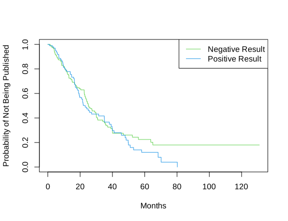
plot(fit.posres), lab-r-km-posres.svg.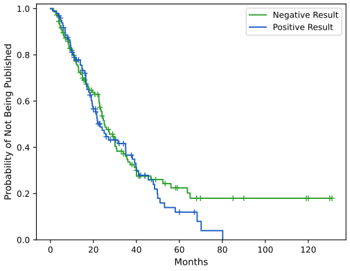
lab-py-km-posres.svg.11.8.3 Call Center Data
pp. 487–490 2000 simulated calls. The predictors are the number of operators available (5 to 15), the call centre (A, B or C) and the time of day (morning, afternoon, evening), all equally likely. The wait until the call is answered follows a Cox model with baseline hazard \(h_0(t)=10^{-5}t\) and coefficients 0.04 (operators), \(-0.3\) (centre B), 0 (centre C), 0.2 (evening) and \(-0.2\) (morning): each extra operator multiplies the rate of being answered by \(e^{0.04}=1.041\), and centre B answers at \(e^{-0.3}=0.74\) times the rate of centre A. Since \(S(t\given x)=\exp(-H_0(t)e^{x^\T\beta})\) with \(H_0(t)=10^{-5}t^2/2\), a uniform \(U\) gives a waiting time \(H_0^{-1}(-\log U/e^{x^\T\beta})=\sqrt{2(-\log U)/(10^{-5}e^{x^\T\beta})}\) (inverse-transform sampling, Result 11.3). Waits are capped at 1000 seconds, and 10% of the calls, chosen at random, are marked as hang-ups (censored).
R
set.seed(4)
N <- 2000
Operators <- sample(5:15, N, replace = TRUE)
Center <- sample(c("A", "B", "C"), N, replace = TRUE)
Time <- sample(c("Morn.", "After.", "Even."), N, replace = TRUE)
X <- model.matrix(~ Operators + Center + Time)[, -1]
print(X[1:5, ])

true.beta <- c(0.04, -0.3, 0, 0.2, -0.2)
h.fn <- function(x) 0.00001 * x               # the baseline hazard h0(t)
H.fn <- function(x) 0.00001 * x^2 / 2         # its integral, the cumulative baseline hazard H0(t)
# Under proportional hazards S(t | x) = exp(-H0(t) exp(x'beta)), so with U uniform the time
# H0^{-1}(-log(U) / exp(x'beta)) has survival function S(t | x)  (inverse-transform sampling)
lin.pred <- drop(X %*% true.beta)
wait <- sqrt(2 * (-log(runif(N))) / (0.00001 * exp(lin.pred)))
y <- pmin(wait, 1000)                         # waits are capped at 1000 seconds
failed <- rbinom(N, 1, 0.9) == 1              # 90% of calls answered, 10% hang-ups (censored)
queuing <- data.frame(X, y = y, failed = failed)
print(head(queuing))
print(mean(queuing$failed))
write.csv(queuing, file.path("cache", "ch11_callcenter_R.csv"), row.names = FALSE)
Python
rng = np.random.default_rng(10)
N = 2000
Operators = rng.choice(np.arange(5, 16), N, replace=True)
Center = rng.choice(["A", "B", "C"], N, replace=True)
Time = rng.choice(["Morn.", "After.", "Even."], N, replace=True)
D = pd.DataFrame({"Operators": Operators, "Center": Center, "Time": Time})
X = model_matrix(D, ["Operators", "Center", "Time"])          # baselines: Center A, afternoon
print(X[:5])

true_beta = np.array([0.04, -0.3, 0, 0.2, -0.2])
true_linpred = X.to_numpy() @ true_beta
hazard = lambda t: 1e-5 * t                                   # noqa: E731  baseline hazard h0(t)
cum_hazard = lambda t: 1e-5 * t ** 2 / 2                      # noqa: E731  H0(t), its integral
# S(t | x) = exp(-H0(t) exp(x'beta)): with U uniform, H0^{-1}(-log(U) / exp(x'beta)) has this law
U = rng.uniform(size=N)
W = np.sqrt(2 * (-np.log(U)) / (1e-5 * np.exp(true_linpred)))
assert np.allclose(cum_hazard(W) * np.exp(true_linpred), -np.log(U)) and hazard(1.0) == 1e-5
D["Wait time"] = np.clip(W, 0, 1000)                          # waits are capped at 1000 seconds
D["Failed"] = rng.choice([1, 0], N, p=[0.9, 0.1])             # 1 = answered, 0 = hung up (censored)
print(D[:5])
print("share answered: %.4f" % D["Failed"].mean())
R: Operators CenterB CenterC TimeEven. TimeMorn. y failed
1 12 1 0 0 1 344.294 FALSE
2 15 0 0 0 0 240.951 FALSE
3 7 0 1 1 0 186.504 TRUE
mean(failed) = 0.897
Python: Operators Center Time Wait time Failed
0 13 C After. 525.064979 1
1 15 A Even. 254.677835 1
2 7 B Morn. 487.739224 1
share answered: 0.9075
The R lab's first rows have the same predictors and, to the second, the same waiting times as the book's R output (344, 241, 187, ...), but different hang-up flags, so its counts differ from the book's. The Python lab's wait times are those printed in the Python edition.
Kaplan–Meier curves by centre and by time of day, and log-rank tests for three groups.
R
queuing$Center <- Center                      # the group labels, for the stratified curves and tests
queuing$Time <- Time
fit.Center <- survfit(Surv(y, failed) ~ Center, data = queuing)
fit.Time <- survfit(Surv(y, failed) ~ Time, data = queuing)
open_svg("lab-r-callcenter", width = 9, height = 4.2)
par(mfrow = c(1, 2))
plot(fit.Center, xlab = "Seconds", ylab = "Probability of Still Being on Hold", col = c(2, 4, 5))
legend("topright", c("Call Center A", "Call Center B", "Call Center C"), col = c(2, 4, 5), lty = 1)
plot(fit.Time, xlab = "Seconds", ylab = "Probability of Still Being on Hold", col = c(2, 4, 5))
legend("topright", c("Afternoon", "Evening", "Morning"), col = c(2, 4, 5), lty = 1)
dev.off()

lr.center <- survdiff(Surv(y, failed) ~ Center, data = queuing)
lr.time <- survdiff(Surv(y, failed) ~ Time, data = queuing)
print(lr.center)
print(lr.time)
lrt <- function(fit) 2 * diff(fit$loglik)
cat("LR tests: Center", lrt(coxph(Surv(y, failed) ~ Center, data = queuing)),
    " Time", lrt(coxph(Surv(y, failed) ~ Time, data = queuing)), "\n")
Python
fig, axes = figure(width=9.0, height=4.2, ncols=2)
for ax, var, labels in ((axes[0], "Center", ["A", "B", "C"]), (axes[1], "Time", ["After.", "Even.", "Morn."])):
    for lv, colour in zip(labels, (common.RED, common.BLUE, common.CYAN)):
        part = D[D[var] == lv]
        step_plot(ax, km_table(part["Wait time"], part["Failed"]), colour, label="%s = %s" % (var, lv), marks=False)
    ax.legend(loc="upper right")
    ax.set(xlabel="Seconds", ylabel="Probability of Still Being on Hold", ylim=(0, 1.02))
common.savefig(fig, 11, "lab-py-callcenter", formats=("svg",))

lr_center = logrank_test(D["Wait time"], D["Failed"], D["Center"])
lr_time = logrank_test(D["Wait time"], D["Failed"], D["Time"])
print(lr_center["table"].round(3)); print("Chisq = %.2f on 2 df, p = %.2g" % (lr_center["chisq"], lr_center["p"]))
print(lr_time["table"].round(3)); print("Chisq = %.2f on 2 df, p = %.2g" % (lr_time["chisq"], lr_time["p"]))

LR_center = coxph(D["Wait time"], D["Failed"], model_matrix(D, ["Center"]))[1]["tests"]["LR"]
LR_time = coxph(D["Wait time"], D["Failed"], model_matrix(D, ["Time"]))[1]["tests"]["LR"]
print("LR tests: Center %.2f, Time %.2f" % (LR_center, LR_time))
R (its own data): Center chisq 34.4, p = 3e-08; Time chisq 42.9, p = 5e-10
Cox LR tests: Center 35.25, Time 42.06
Python (the Python edition's data):
N Observed Expected (O-E)^2/E (O-E)^2/V
A 684 614.0 577.874 2.258 3.331
B 649 597.0 688.419 12.140 19.880
C 667 604.0 548.707 5.572 8.053
Chisq = 20.30 on 2 df, p = 3.9e-05
Chisq = 49.90 on 2 df, p = 1.5e-11 (time of day)
LR tests: Center 20.58, Time 48.12
Centre B and the morning have the longest waits, the evening the shortest, and both differences are highly significant. As in the two-group case, the log-rank and Cox likelihood ratio statistics are close.
Cox's model with all three predictors recovers the true coefficients (0.04, \(-0.3\), 0, 0.2, \(-0.2\)) within about two standard errors.
R
fit.queuing <- coxph(Surv(y, failed) ~ Operators + CenterB + CenterC + TimeEven. + TimeMorn.,
                     data = queuing)
print(fit.queuing)
Python
fit_queuing, res_queuing = coxph(D["Wait time"], D["Failed"], X)
print(res_queuing["table"].round(5))
R (its data) Python (Python edition's data)
coef se(coef) coef se(coef)
Operators 0.04114 0.00756 0.04393 0.00752
CenterB -0.27720 0.05765 -0.23606 0.05811
CenterC 0.04183 0.05793 0.01223 0.05752
TimeEven. 0.20879 0.05812 0.26884 0.05780
TimeMorn. -0.15537 0.05780 -0.14822 0.05733
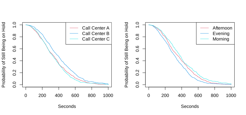
lab-r-callcenter.svg.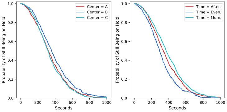
lab-py-callcenter.svg.One feature of this simulation, shared by both editions: a hang-up keeps the call's own answer time as its observed time. A real hang-up would happen before the answer. Marking 10% of the event times as censored at random thins the observed events but leaves the risk sets unchanged, so the hazard of an observed answer is \(0.9\,h(t\given x)\): still proportional, so Cox's coefficients are estimated without bias, but the Kaplan–Meier curves estimate \(S(t)^{0.9}\) rather than \(S(t)\). At 300 seconds the curve of all calls is at 0.570, while the true probability of still waiting is 0.540 (Notes on the book).
Notes on the book
Publication data: impact is measured after the outcome
impact is described as "related to the number of citations". It is 0 for 87 of the 88 unpublished (censored) trials and positive for 146 of the 156 published ones: an unpublished trial has nothing to cite. So it is not a characteristic of the trial at time zero, and its enormous effect in Tables 11.3 and in the lab (\(z=8.7\)), the selection of impact by the lasso, the separation of Figure 11.8 and the C-index of Section 11.7.1 all partly reflect the outcome itself. The book's main conclusion about posres survives without it: with posres, multi, clinend, sampsize and budget only, the coefficient of posres is 0.536 (\(p=0.003\)).
Table 11.3: two coefficients are not estimates
The rows mech[R42] (−14.78, standard error 3414.38) and mech[RC2] (−14.92, 2243.60) belong to funding mechanisms with one trial each, neither published. Their partial likelihood increases without bound as the coefficient decreases, so the maximum likelihood estimate is \(-\infty\); R stops at about −15 and prints the warning "coefficient may be infinite" (Filling the gap 11.14). They should be reported as not estimable, or the two trials removed, which leaves the other rows unchanged.
Figure 11.7: the horizontal axis divides by a norm that does not exist
The axis of Figure 11.7 is \(\|\hat\beta^L_\lambda\|_1/\|\hat\beta\|_1\), with \(\hat\beta\) the unpenalised Cox fit. On these data that fit has coefficients diverging to \(-\infty\) (the previous note), so \(\|\hat\beta\|_1\) is whatever number the optimiser stopped at, at least about 30 from the two diverging coefficients alone. This is why the book's axis runs from \(2\times10^{-4}\) to only 0.2 and the minimum sits at \(1.7\times10^{-3}\): the ratio is not the usual "fraction of the full fit" that runs up to 1. Figure 11.7 here uses \(\lambda\) instead.
"Exactly equal" to the log-rank test needs untied times
Section 11.5.2 states that the score test for a single binary covariate is exactly the log-rank test. That is true for the brain cancer data (1.44049511 in both, the R lab) because no two deaths share a time. With tied times, Cox's partial likelihood needs an approximation, and the score tests of Breslow's and Efron's approximations differ slightly from the log-rank statistic: on the Publication data 0.8430 (Breslow) and 0.8409 (Efron, R's default) against 0.8440. The equality is restored by the exact discrete-time partial likelihood (coxph(..., ties = "exact") gives 0.8440).
The R lab's "additional digits" of the Wald test are still rounded
After noting that the printed tests are rounded, the R lab prints summary(fit.cox)$waldtest[1] as 1.4200000. summary.coxph() stores the Wald statistic already rounded to two decimals; the statistic itself is \((0.407669/0.342004)^2=1.4209\) (fit.cox$wald.test). The likelihood ratio (1.4388222) and score (1.44049511) values are not rounded.
The Python lab compares the wrong test with the log-rank statistic
The Python lab prints the log-rank statistic 1.44 (In[9]) and the Cox likelihood ratio statistic 1.44 (In[11]) and concludes that "the score test from the Cox model is exactly equal to the log rank test statistic". The two printed numbers are 1.4405 and 1.4388; they agree only after rounding. The score test, which the lab never computes, is the one equal to the log-rank statistic (1.44049511).
The Python lab's default confidence level
The Python lab says that KaplanMeierFitter draws "90% confidence intervals" by default. The lifelines documentation gives alpha=0.05 as the default, i.e. 95% intervals, consistent with the lab's own instruction to set alpha to one minus the confidence level.
The Python lab's share of answered calls
Out[28] of the Python lab prints D['Failed'].mean() as 0.8985. The data the lab analyses afterwards have 1815 answered calls, a share of 0.9075: with exactly these data (the same seed and the same wait times as Out[27]) the lab here reproduces the Python edition's log-rank statistics (20.30 and 49.90) and likelihood ratio statistics (20.58 and 48.12) to all printed digits and its Cox coefficients (0.043934, −0.236059, ...) to within \(3\times10^{-6}\) (the optimisers stop at slightly different points), and the observed counts of the log-rank tables add up to 1815.
The simulated hang-ups are not censoring times
Both labs mark 10% of the calls, chosen at random, as hang-ups (censored), but keep the call's answer time as the observed time. A caller who hangs up does so before the call would have been answered, so the observed time of a hang-up should be earlier than the wait. With this scheme the observed answers have hazard \(0.9\,h(t\given x)\): Cox's coefficients are unaffected (the factor 0.9 is absorbed in the baseline), but the Kaplan–Meier curves of the lab estimate \(S(t)^{0.9}\), not the probability of still being on hold. At 300 seconds: 0.570 from Kaplan–Meier, against 0.540 for the true \(S(300)\) averaged over the callers (0.574 for \(S^{0.9}\)). Drawing an independent hang-up time \(C\) and observing \(\min(T,C)\) would follow Definition 11.1.
Exercise 11: the covariate value 11 in Table 11.4
The second row of Table 11.4 has \(X=11\), far from the other values (−0.3 to 2.8); both editions print it so, and it is used as printed here. If it were 1.1, group 2 (\(X\ge2\)) would contain a single censored observation and no death, and the Cox coefficient of part (b) would have no finite estimate (the situation of Filling the gap 11.14).
Figure 11.2: the band is a 95% confidence band
The caption of Figure 11.2 speaks of "standard error bands". The dashed curves are R's default pointwise 95% confidence interval on the log scale, \(\hat S(t)e^{\pm1.96\,\mathrm{se}}\) (Filling the gap 11.4): at 20 months they are at 0.620 and 0.820, while \(\hat S\pm1\) standard error, the band Exercise 10(a) asks for, would be 0.662 and 0.764.
Exercises
Conceptual exercises 1–9 and applied exercises 10–11, in the book's numbering (the two editions have the same exercises). The applied solutions are the last sections of ch11_lab.R and ch11_lab.py.
Exercise 11.1. Is the censoring independent? (a) Patients whose phone number starts with 2 are lost to follow-up. (b) Ages above 99 are lost (known to exceed 99). (c) Very sick patients are transferred to another hospital and lost. (d) People who find work early stop answering an unemployment study. (e) Pre-term deliveries happen more often away from the usual hospital and are censored more often. (f) Residents who study out of town are lost more often and are more likely to attend graduate school. (g) Patients without relapse after five years are considered cured and censored at five years. (h) Components from two factories of equal quality are censored at five and at two years. (i) The same, but the older factory makes better components.
Solution
The question each time: once the predictors are fixed, does the censoring time tell us anything about the survival time? (a) Independent: the first digit of a phone number has nothing to do with relapse. (b) Independent: every person is censored at the same fixed value 99 (like the end of a study), which does not depend on their lifetime; this is ordinary right censoring at a known point. (c) Not independent: those censored are the sickest, so the remaining patients overstate survival. (d) Not independent: censoring is linked to short unemployment, so durations will be overestimated. (e) Not independent: censoring is more likely for short pregnancies. (f) Not independent: those lost to follow-up are those with longer education. (g) Independent: censoring at a fixed five years for everyone is administrative; whether "cured" is the right interpretation is a separate question. (h) Independent: the censoring time depends on the factory, but the factory is unrelated to the failure time. (i) Not independent marginally: the censoring time (through the factory) is related to quality and so to the failure time. It is independent conditional on the factory, so the methods of the chapter apply if the factory is included as a predictor (or as strata).
Exercise 11.2. Four people are followed for two years after buying a phone: (1) replaces it after 1.2 years; (2) has not replaced it at the end of the study; (3) is lost to follow-up at 1.5 years, not having replaced it; (4) replaces it after 0.2 years. For each: (a) censored? (b) \(c_i\)? (c) \(t_i\)? (d) \(y_i\)? (e) \(\delta_i\)?
Solution
\(i\) (a) censored (b) \(c_i\) (c) \(t_i\) (d) \(y_i\) (e) \(\delta_i\) 1 no not observed (at least 1.2; 2 if only the end of the study could have censored it) 1.2 1.2 1 2 yes 2 unknown, \(\gt2\) 2 0 3 yes 1.5 unknown, \(\gt1.5\) 1.5 0 4 no not observed 0.2 0.2 1 \(y_i\) and \(\delta_i\) are always known; exactly one of \(t_i\), \(c_i\) is.
Exercise 11.3. For Exercise 2, give \(K\), the \(d_k\), \(r_k\) and \(q_k\).
Solution
Two replacement times: \(K=2\), \(d_1=0.2\), \(d_2=1.2\). At 0.2 all four are at risk (\(r_1=4\), \(q_1=1\)); at 1.2 participants 1, 2 and 3 are (\(r_2=3\), \(q_2=1\)). Hence \(\hat S(t)=1\) before 0.2, \(3/4\) on \([0.2,1.2)\) and \(3/4\cdot2/3=1/2\) from 1.2 on.
Exercise 11.4. The Kaplan–Meier curve of Figure 11.9 comes from the six observations of Table 11.4: \(y=\) 26.5, 37.2, 57.3, 90.8, 20.2, 89.8 with \(\delta=\) 1, 1, 1, 0, 0, 0. (a) What is the estimated probability of surviving past 50 days? (b) Write out \(\hat S(t)\).
Solution
Deaths at 26.5, 37.2 and 57.3; the censoring at 20.2 removes one patient before the first death. Risk sets 5, 4, 3. (a) \(\hat S(50)=\frac45\cdot\frac34=0.6\). (b)
\[ \hat S(t)=\begin{cases}1&t\lt26.5\\0.8&26.5\le t\lt37.2\\0.6&37.2\le t\lt57.3\\0.4&57.3\le t\ (\text{up to }90.8,\text{ the largest time}).\end{cases} \]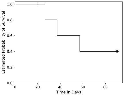
Figure 11.9. Kaplan–Meier curve of the six observations of Table 11.4; + marks censored times. Code: fig_11_9. Reproduces James et al. (2021), Figure 11.9. Download: PDF · SVGExercise 11.5. Sketch \(\hat S(t)=0.8\) for \(t\lt31\), \(0.5\) for \(31\le t\lt77\), \(0.22\) for \(77\le t\).
Solution
A right-continuous step function: a horizontal segment at 0.8 from 0 to 31 (open circle at the right end), a drop to 0.5 at 31 (filled dot at \((31,0.5)\)), flat to 77, a drop to 0.22 at 77, flat afterwards. The conditional survival factors are \(0.5/0.8=0.625\) at 31 and \(0.22/0.5=0.44\) at 77. Unlike a Kaplan–Meier curve it starts at 0.8 rather than 1, as if 20% of the patients had died at time 0; it is an illustration of the shape, as the book says.
Exercise 11.6. For the four patients of Figure 11.1: (a) give \(\delta_i\), \(K\), \(d_k\), \(r_k\), \(q_k\); (b) sketch the Kaplan–Meier curve; (c) the probability that the event occurs within 200 days, and that it does not occur within 310 days; (d) write out \(\hat S(t)\).
Solution
(a) \(\delta=(1,0,1,0)\); the order of the times is \(y_3\lt y_4\lt y_1\lt y_2\). \(K=2\), \(d_1=y_3\), \(d_2=y_1\); at \(y_3\) all four are at risk (\(r_1=4\)), at \(y_1\) only patients 1 and 2 (patient 4 was censored before): \(r_2=2\); \(q_1=q_2=1\).
(b), (d) \(\hat S(t)=1\) for \(t\lt y_3\), \(3/4\) for \(y_3\le t\lt y_1\), \(\frac34\cdot\frac12=3/8\) for \(y_1\le t\le y_2\). The drop at \(y_1\) is larger than at \(y_3\) because the risk set has shrunk.
(c) With \(y_3=150\) and \(y_1=300\) (Figure 11.1): \(\Pr(T\le200)=1-\hat S(200)=1/4\), \(\Pr(T\gt310)=\hat S(310)=3/8\).
Exercise 11.7. (a) Argue that under equal survival \(q_{1k}\) is hypergeometric, and give its parameters. (b) Derive its mean and variance and compare with (11.5)–(11.6).
Solution
See Result 11.2 and Filling the gap 11.6: \(q_{1k}\) is the number of group-1 members among \(q_k\) draws without replacement from \(r_k\) individuals, \(r_{1k}\) of them in group 1; mean \(q_kr_{1k}/r_k\), which is (11.5), and variance \(q_k\frac{r_{1k}}{r_k}\big(1-\frac{r_{1k}}{r_k}\big)\frac{r_k-q_k}{r_k-1}\), which is (11.6).
Exercise 11.8. With \(F=1-S\), show that \(f(t)=dF(t)/dt\) and \(S(t)=\exp\big(-\int_0^th(u)\,du\big)\).
Solution
See Result 11.3 and Filling the gap 11.8.
Exercise 11.9. Exponential survival times. (a) Show \(S(t)=e^{-\lambda t}\). (b) Write the likelihood (11.13) for \(n\) independent times. (c) Show \(\hat\lambda=\sum\delta_i/\sum y_i\). (d) Estimate the mean survival time.
Solution
(a) \(S(t)=1-\int_0^t\lambda e^{-\lambda u}du=e^{-\lambda t}\); equivalently \(h=f/S=\lambda\) and \(S=\exp(-\int_0^t\lambda)\). (b) \(L(\lambda)=\prod_i(\lambda e^{-\lambda y_i})^{\delta_i}(e^{-\lambda y_i})^{1-\delta_i}=\lambda^{\sum\delta_i}e^{-\lambda\sum y_i}\). (c) \(\frac{d}{d\lambda}\log L=\frac{\sum\delta_i}{\lambda}-\sum y_i=0\) gives \(\hat\lambda\); the second derivative \(-\sum\delta_i/\lambda^2\) is negative. (d) The mean of \(\mathrm{Exp}(\lambda)\) is \(1/\lambda\), and by invariance of maximum likelihood its estimate is \(\sum_iy_i/\sum_i\delta_i\): total follow-up time divided by the number of deaths. For the brain cancer data, 69.0 months (Result 11.4). The standard error of \(\hat\lambda\) is about \(\hat\lambda/\sqrt{\sum\delta_i}\): the precision depends on the number of deaths, not on \(n\).
Exercise 11.10. Brain cancer data. (a) Plot the Kaplan–Meier curve with \(\pm1\) standard error bands. (b) Estimate the standard error of the curve at each time by the bootstrap (\(B=200\) resamples of the pairs \((y_i,\delta_i)\)) and compare with (a). (c) Fit a Cox model with all predictors and summarise. (d) Stratify by the Karnofsky index (with ki = 40 merged into ki = 60) and plot the survival curves of the five strata adjusted for the other predictors.
Solution
R
km.se <- summary(fit.surv)$std.err
open_svg("lab-r-ex10a")
plot(fit.surv, conf.int = FALSE, xlab = "Months", ylab = "Estimated Probability of Survival")
lines(stepfun(fit.surv$time, c(1, fit.surv$surv + fit.surv$surv * fit.surv$std.err)), lty = 2,
      do.points = FALSE)
lines(stepfun(fit.surv$time, c(1, fit.surv$surv - fit.surv$surv * fit.surv$std.err)), lty = 2,
      do.points = FALSE)
dev.off()

km_at <- function(time, status, t) {
  f <- survfit(Surv(time, status) ~ 1)
  stepfun(f$time, c(1, f$surv))(t)
}
set.seed(1)
tt <- c(10, 20, 40, 60)
boot <- replicate(200, {
  i <- sample(nrow(BrainCancer), replace = TRUE)
  km_at(BrainCancer$time[i], BrainCancer$status[i], tt)
})
print(rbind(greenwood = summary(fit.surv, times = tt)$std.err, bootstrap = apply(boot, 1, sd)))

BrainCancer$ki5 <- ifelse(BrainCancer$ki == 40, 60, BrainCancer$ki)
fit.ki <- coxph(Surv(time, status) ~ sex + diagnosis + loc + gtv + stereo + strata(ki5),
                data = BrainCancer)
print(fit.ki)
typical <- data.frame(sex = "Female", diagnosis = "Meningioma", loc = "Supratentorial",
                      gtv = mean(BrainCancer$gtv), stereo = "SRT")
surv.ki <- survfit(fit.ki, newdata = typical)
open_svg("lab-r-ex10d")
plot(surv.ki, col = 2:6, xlab = "Months", ylab = "Survival Probability")
legend("bottomleft", paste("ki =", sort(unique(BrainCancer$ki5))), col = 2:6, lty = 1)
dev.off()
Python
# (a) +/- 1 standard error bands
fig, ax = figure()
x = np.r_[0.0, km_all["time"]]
ax.step(x, np.r_[1.0, km_all["surv"]], where="post", color="k", lw=1.4)
for sign in (1, -1):
    ax.step(x, np.r_[1.0, km_all["surv"] + sign * km_all["se_S"]], where="post", color="k", lw=0.9, ls="--")
ax.set(xlabel="Months", ylabel="Estimated Probability of Survival", ylim=(0, 1.02))
common.savefig(fig, 11, "lab-py-ex10a", formats=("svg",))
tt = np.array([10, 20, 40, 60])
greenwood = km_at(km_all, tt, "se_S")

# (b) bootstrap standard errors of S(t), B = 200 resamples of the pairs (y_i, delta_i)
rng = np.random.default_rng(1)
y, delta = BrainCancer["time"].to_numpy(), BrainCancer["status"].to_numpy()
boot = np.array([km_at(km_table(y[i], delta[i]), tt)
                 for i in (rng.integers(0, len(y), len(y)) for _ in range(200))])
print(pd.DataFrame({"greenwood": greenwood, "bootstrap": boot.std(axis=0, ddof=1)}, index=tt).round(4))

# (d) strata of the Karnofsky index (40 merged with 60), adjusted for the other predictors
cc = BrainCancer.dropna().copy()
cc["ki5"] = np.where(cc["ki"] == 40, 60, cc["ki"])
Xs = model_matrix(cc, ["sex", "diagnosis", "loc", "gtv", "stereo"])
model = PHReg(cc["time"].to_numpy(), Xs.to_numpy(), status=cc["status"].to_numpy(),
              strata=cc["ki5"].to_numpy(), ties="efron")
fs = model.fit()
print(pd.DataFrame({"coef": fs.params, "se(coef)": fs.bse}, index=Xs.columns).round(4))
typical = np.zeros(Xs.shape[1])                     # female, meningioma, infratentorial, SRS
typical[list(Xs.columns).index("locSupratentorial")] = 1.0
typical[list(Xs.columns).index("stereoSRT")] = 1.0
typical[list(Xs.columns).index("gtv")] = BrainCancer["gtv"].mean()
fig, ax = figure()
s30 = []
colours = (common.RED, common.GREEN, common.BLUE, common.ORANGE, common.PURPLE)
for level, colour in zip(sorted(cc["ki5"].unique()), colours):
    rows = (cc["ki5"] == level).to_numpy()          # each stratum has its own baseline hazard
    tk, Sk = cox_survival(cc["time"][rows], cc["status"][rows], Xs[rows], fs.params, typical[None, :])
    ax.step(np.r_[0.0, tk], np.r_[1.0, Sk[:, 0]], where="post", color=colour, label="ki = %d" % level)
    s30.append(Sk[np.searchsorted(tk, 30, side="right") - 1, 0] if (tk <= 30).any() else 1.0)
ax.legend(loc="lower left")
ax.set(xlabel="Months", ylabel="Survival Probability", ylim=(0, 1.02))
common.savefig(fig, 11, "lab-py-ex10d", formats=("svg",))
print("Exercise 10(d): S(30 months) by ki stratum", np.round(s30, 4))
standard error of S(t) at 10, 20, 40, 60 months Greenwood (both) 0.0420 0.0509 0.0623 0.0736 bootstrap, R 0.0447 0.0505 0.0642 0.0745 bootstrap, Python 0.0408 0.0495 0.0575 0.0663 (d) coefficients (R = Python): sexMale 0.307, LG glioma 0.858, HG glioma 2.244, Other 1.187, Supratentorial 0.686, gtv 0.032, SRT 0.049 S(30 months) for a typical patient, ki 60 / 70 / 80 / 90 / 100: 0.847 0.860 0.851 0.909 1.000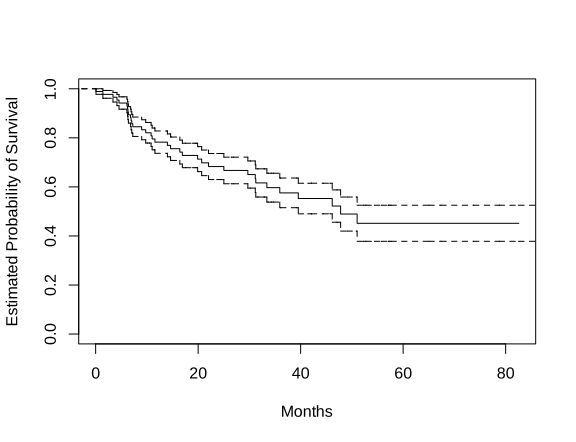
R: (a), lab-r-ex10a.svg.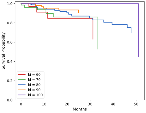
Python: (d), lab-py-ex10d.svg.(a) The \(\pm1\) standard error band is narrower than the 95% band of Figure 11.2 (0.662 to 0.764 at 20 months). (b) The bootstrap standard errors agree with Greenwood's formula to within about 10%. The two languages draw different resamples, and with \(B=200\) a bootstrap standard error has a Monte Carlo error of about \(1/\sqrt{2B}=5\%\) of its value, so differences of this size between the two runs, and between either run and Greenwood, are expected. (c) The fit is Table 11.2: after adjustment, a high-grade glioma multiplies the hazard by 8.6 relative to a meningioma, and each point of the Karnofsky index lowers it by 5%; sex, location, tumour volume and the radiation method show no clear effect (Section 11.5.3). (d) A stratified Cox model (
strata(ki5)) gives each Karnofsky level its own baseline hazard, so no proportionality is assumed between the strata. For a typical patient (female, meningioma, supratentorial, mean tumour volume, SRT) the estimated survival at 30 months is 0.85, 0.86, 0.85, 0.91 and 1.00 for ki = 60, 70, 80, 90 and 100. The strata are small (6 patients in the lowest, 5 in the highest, whose single death is at 51 months), so the curves are rough and show no clean ordering beyond 30 months; the other coefficients change little from (c).Exercise 11.11. Using Table 11.4, with group 1 for \(X\lt2\) and group 2 for \(X\ge2\): (a) plot the two Kaplan–Meier curves; (b) fit Cox's model with the group indicator and interpret the coefficient; (c) run the log-rank test and compare its p-value with the score test of (b).
Solution
R
ex11 <- data.frame(y = c(26.5, 37.2, 57.3, 90.8, 20.2, 89.8),
                   delta = c(1, 1, 1, 0, 0, 0),
                   x = c(0.1, 11, -0.3, 2.8, 1.8, 0.4))
ex11$group <- ifelse(ex11$x < 2, 1, 2)
km11 <- survfit(Surv(y, delta) ~ group, data = ex11)
print(summary(km11))
open_svg("lab-r-ex11")
plot(km11, col = c(2, 4), xlab = "Time in Days", ylab = "Estimated Probability of Survival")
legend("bottomleft", c("Group 1 (X < 2)", "Group 2 (X >= 2)"), col = c(2, 4), lty = 1)
dev.off()
cox11 <- coxph(Surv(y, delta) ~ I(group == 2), data = ex11)
print(summary(cox11))
lr11 <- survdiff(Surv(y, delta) ~ group, data = ex11)
print(lr11)
Python
ex11 = pd.DataFrame({"y": [26.5, 37.2, 57.3, 90.8, 20.2, 89.8], "delta": [1, 1, 1, 0, 0, 0],
                     "x": [0.1, 11, -0.3, 2.8, 1.8, 0.4]})
ex11["group"] = np.where(ex11["x"] < 2, 1, 2)
fig, ax = figure()
for k, colour in ((1, common.RED), (2, common.BLUE)):
    part = ex11[ex11["group"] == k]
    tab = km_table(part["y"], part["delta"])
    print("group %d\n" % k, tab[["time", "n_risk", "n_event", "surv"]])
    step_plot(ax, tab, colour, label="Group %d (%s)" % (k, "X < 2" if k == 1 else "X >= 2"))
ax.legend(loc="lower left")
ax.set(xlabel="Time in Days", ylabel="Estimated Probability of Survival", ylim=(0, 1.02))
common.savefig(fig, 11, "lab-py-ex11", formats=("svg",))
fit11, res11 = coxph(ex11["y"], ex11["delta"], (ex11["group"] == 2).astype(float).to_frame("group2"))
lr11 = logrank_test(ex11["y"], ex11["delta"], ex11["group"])
print(res11["table"].round(4))
print("score test %.6f, log-rank %.6f, p = %.4f" % (res11["tests"]["score"], lr11["chisq"], lr11["p"]))
group 1 (X < 2, 4 observations): S = 0.667 from 26.5, 0.333 from 57.3 group 2 (X >= 2, 2 observations): S = 0.5 from 37.2 Cox: coef -0.340, exp(coef) 0.712, se 1.236, z -0.28, p 0.78 score test 0.076443 = log-rank chi-squared 0.076443, p = 0.782
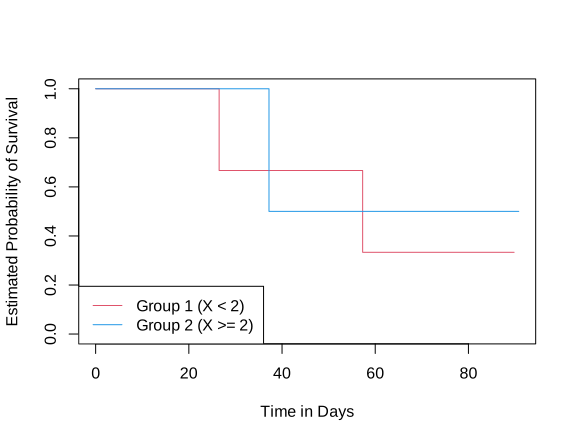
R: lab-r-ex11.svg.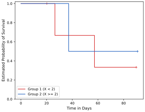
Python: lab-py-ex11.svg.(a) Group 1 ends lower (0.33 against 0.5), but with four and two observations the curves say almost nothing. (b) \(\hat\beta=-0.340\): the estimated hazard in group 2 is \(e^{-0.340}=0.71\) times that of group 1 at every time, a 29% lower instantaneous risk. Its standard error 1.24 (\(p=0.78\)) gives no evidence that the true coefficient differs from 0. (c) The log-rank statistic is 0.0764 with \(p=0.782\), identical to the Cox score test: there are no tied death times, as Result 11.7 requires. The Wald p-value 0.78 is close too. The data as printed have \(X=11\) in the second row (Notes on the book).
Demonstrations for this chapter
Each demonstration runs in the browser on the book's data and links back to these notes. The ▶ Demo boxes above open them already set to the case under discussion.
| Demonstration | What you can see | Sections |
|---|---|---|
| Kaplan–Meier curves with censoring | The curves of the brain cancer data by any grouping, with censoring marks, the 95% band, the risk set and the conditional factor at any time, the two naive estimates and the redistribution of censored mass. Presets: 1 all patients; 2 by sex; 3 by diagnosis; 4 naive estimates at 20 months; 5 redistribution to the right. | 11.3, 11.4 |
| The log-rank test as observed minus expected | The 2×2 table at every death time with its hypergeometric mean and variance, the running sum of observed minus expected deaths with its \(\pm1.96\) standard-deviation envelope, and a permutation distribution. Presets: 1 sex; 2 the first death; 3 high-grade glioma against the rest; 4 publication by result (tied times); 5 permutation test. | 11.4 |
| The Cox partial likelihood for one predictor | The log partial likelihood curve, the probabilities (11.15) of each patient at risk at a chosen death, Newton's steps, and the likelihood ratio, Wald and score tests, with Breslow's or Efron's ties. Presets: 1 sex; 2 the score test is the log-rank test; 3 the Karnofsky index; 4 publication by result, Breslow against Efron; 5 Newton's method for impact. | 11.5.2 |
References
- James, G., Witten, D., Hastie, T. and Tibshirani, R. (2021). An Introduction to Statistical Learning with Applications in R, 2nd edition. Springer, New York. Chapter 11, pp. 461–495. www.statlearning.com.
- James, G., Witten, D., Hastie, T., Tibshirani, R. and Taylor, J. (2023). An Introduction to Statistical Learning with Applications in Python. Springer, Cham. Chapter 11.
- Breslow, N. (1974). Covariance analysis of censored survival data. Biometrics, 30, 89–99.
- Cox, D. R. (1972). Regression models and life-tables (with discussion). Journal of the Royal Statistical Society, Series B, 34, 187–220.
- Cox, D. R. (1975). Partial likelihood. Biometrika, 62, 269–276.
- Efron, B. (1967). The two sample problem with censored data. Proceedings of the Fifth Berkeley Symposium on Mathematical Statistics and Probability, 4, 831–853.
- Efron, B. (1977). The efficiency of Cox's likelihood function for censored data. Journal of the American Statistical Association, 72, 557–565.
- Gordon, D., Taddei-Peters, W., Mascette, A., Antman, M., Kaufmann, P. G. and Lauer, M. S. (2013). Publication of trials funded by the National Heart, Lung, and Blood Institute. New England Journal of Medicine, 369, 1926–1934.
- Greenwood, M. (1926). The natural duration of cancer. Reports on Public Health and Medical Subjects, 33, 1–26.
- Harrell, F. E., Califf, R. M., Pryor, D. B., Lee, K. L. and Rosati, R. A. (1982). Evaluating the yield of medical tests. Journal of the American Medical Association, 247, 2543–2546.
- Heagerty, P. J., Lumley, T. and Pepe, M. S. (2000). Time-dependent ROC curves for censored survival data and a diagnostic marker. Biometrics, 56, 337–344.
- Ishwaran, H., Kogalur, U. B., Blackstone, E. H. and Lauer, M. S. (2008). Random survival forests. Annals of Applied Statistics, 2, 841–860.
- Johansen, S. (1983). An extension of Cox's regression model. International Statistical Review, 51, 165–174.
- Kaplan, E. L. and Meier, P. (1958). Nonparametric estimation from incomplete observations. Journal of the American Statistical Association, 53, 457–481.
- Mantel, N. (1966). Evaluation of survival data and two new rank order statistics arising in its consideration. Cancer Chemotherapy Reports, 50, 163–170.
- Selingerová, I., Doležalová, H., Horáková, I., Katočová, S., Mach, A., Kouba, M. and Kazda, T. (2016). Survival of patients with primary brain tumors: comparison of two statistical approaches. PLoS One, 11(2), e0148733.
- Simon, N., Friedman, J., Hastie, T. and Tibshirani, R. (2011). Regularization paths for Cox's proportional hazards model via coordinate descent. Journal of Statistical Software, 39(5), 1–13.
- Uno, H., Cai, T., Tian, L. and Wei, L. J. (2007). Evaluating prediction rules for t-year survivors with censored regression models. Journal of the American Statistical Association, 102, 527–537.
- Verweij, P. J. M. and van Houwelingen, H. C. (1993). Cross-validation in survival analysis. Statistics in Medicine, 12, 2305–2314.
The numerical statements in the text (the book's printed tables and tests, the Kaplan–Meier, Greenwood, log-rank and Cox formulas, the score test as the log-rank test, the agreement of the R and Python labs, the lasso fits and the exercise results) were confirmed numerically.