Chapter 12. Supervised Learning
In supervised learning the data carry the answer: for every training object we know the property we want to predict (a diabetes type, a developmental stage, a cancer diagnosis), and we learn a rule that predicts it from the other measurements. This chapter of Holmes and Huber (2019) introduces discriminant analysis, shows how a flexible rule learns its training data by heart, how cross-validation exposes this, why many features are a curse, and how penalisation (ridge, lasso, elastic net) and tuning by cross-validation tame it. The book runs MASS::lda, glmnet and caret and states the theory briefly; these notes derive it: the Bayes rule, the Gaussian class models behind LDA and QDA, the counting theorem that explains learning by heart, the bias of cross-validation, the bias-variance decomposition, the closed form of ridge, soft-thresholding and the coordinate-descent path of the lasso, and the selection bias that hides in every data-driven choice.
Ch. 1 Discrete data Ch. 2 Statistical modeling Ch. 3 Data visualization Ch. 4 Mixture models Ch. 5 Clustering Ch. 6 Testing Ch. 7 Multivariate analysis Ch. 8 Count data and GLMs Ch. 9 Heterogeneous data Ch. 10 Networks and trees Ch. 11 Image data Ch. 12 Supervised learning Ch. 13 Experimental design
How to read these notes
They follow the book. Sections carry the book's numbers (12.3.1, 12.6.2, ...), and the displayed equations that appear in the book carry its equation numbers, e.g. (12.6). In-text questions of the book are restated as Question 12.k boxes with a worked answer; the end-of-chapter exercises are in the Exercises section.
Filling the gaps. The book is applied and leaves most of the theory to Hastie et al. (2008). Wherever it states a result without derivation, an orange Filling the gap box or a proof gives the full argument at the level of a graduate statistics course. Derivations start hidden: open one with its bar, or use the button below. A few places where the book's formula or wording is not correct are marked Note on the text.
Figures, code and demonstrations. All 21 figures of the chapter that are computed from data or by simulation are recomputed by the course's R code (code/ch12_supervised_learning.R); four schematics and photographs (Figures 12.2, 12.4, 12.14, 12.18) are not reproduced. Every derivation below is verified against R packages, brute force or simulation. The ▶ Demo boxes open an interactive demonstration already set to the case under discussion.
Main reference
S. Holmes and W. Huber, Modern Statistics for Modern Biology, Cambridge University Press (2019), Chapter 12. Section, equation, figure, question and exercise numbers refer to this book. The book's own pointer for the theory is Hastie, Tibshirani and Friedman (2008), The Elements of Statistical Learning.
The explanations, derivations and code are my own; results of the book are cited by their numbers.
The chapter at a glance
- 12.2–12.3 A classifier is judged by its risk; the Bayes rule (largest posterior probability) is optimal (Result 12.1). Modelling each class as a Gaussian with a shared covariance gives LDA, whose boundaries are hyperplanes (Result 12.2); separate covariances give QDA with quadratic boundaries and many more parameters (Filling the gap 12.3).
- 12.4 With \(p\ge n-1\) features almost every labelling of \(n\) points is linearly separable (Result 12.4), so a flexible rule fits random labels perfectly; the training error is optimistic by \(2\sigma^2p/n\) in regression (Result 12.5). Leave-one-out cross-validation estimates the error of a rule trained on \(n-1\) points without bias (Result 12.6), but only if every data-driven step, feature selection included, is repeated inside the loop (Filling the gap 12.4). Noise features degrade a real signal (Result 12.8), and high-dimensional space is empty, all shell, and has nearly equal distances (Result 12.9).
- 12.5 Loss functions and the rules that minimise them; sensitivity, specificity, predictive values, ROC curves and the AUC as a Mann-Whitney probability (Results 12.10–12.12).
- 12.6 MSE = noise + bias² + variance (Result 12.13); under 0-1 loss bias can be free (Result 12.14). Logistic regression and its penalised versions: ridge has a closed form and always beats least squares for a small enough penalty (Result 12.15), the lasso soft-thresholds (Result 12.16), and the whole path is computed by coordinate descent from \(\lambda_{\max}\) down (Result 12.17, Algorithm 12.2). Applications to the stool microbiome and to mouse embryo cells.
- 12.7 Nearest neighbours (at most twice the Bayes error, Result 12.18), support vector machines and kernels, tuning with
caret, and the optimism of picking the best of many tries (Result 12.19, Algorithm 12.3).
Notation. Training data \((\x_i,y_i)\), \(i=1,\dots,n\), with \(\x_i\in\R^p\); \(\X\) is the \(n\times p\) matrix with rows \(\x_i^\T\). Classes are \(k=1,\dots,K\) with prior probabilities \(\pi_k\), class-conditional densities \(f_k\) and posterior probabilities \(p_k(\x)=\Pr(Y=k\given X=\x)\). A prediction rule is \(\hat f\) (regression) or \(\hat g\) (classification); \(\Phi\) is the standard normal distribution function; \(\one\{\cdot\}\) is an indicator.
Prerequisites. Multivariate normal distributions and maximum likelihood (Chapters 2, 4 and 7 of the book); generalised linear models and the logistic link (Chapter 8); hypothesis tests and p-value histograms (Chapter 6).
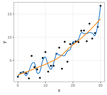
The chapter opens with the central danger of the subject, overfitting. Figure 12.1 fits two smooth curves to the same 31 points: the wiggly one follows the noise and would predict new data worse than the stiff one. Choosing how wiggly a curve may be is a model-selection problem with a tuning parameter (here the loess span), exactly like the penalty \(\lambda\) of Section 12.6.1 (Exercise 12.3).
12.2 What are the data?
The data are a table: one row per object, one column per feature, and one column, the response, singled out to be predicted from the others. A continuous response makes the task regression, a categorical one classification; the difference matters because it changes the loss function (Section 12.5). The book's Figure 12.2 (a schematic, not reproduced) splits the rows into a training set \((X_\ell,Y_\ell)\) used to learn the rule and a test (validation) set \((X_v,Y_v)\) used to judge it.
Definition 12.1 (the supervised learning problem) Section 12.2
Let \((X,Y)\) have a joint distribution \(P\) on \(\R^p\times\mathcal{Y}\), and let the training sample \(D_n=\{(\x_i,y_i)\}_{i=1}^n\) be \(n\) independent draws from \(P\). A learning procedure maps \(D_n\) to a prediction rule \(\hat f=\hat f_{D_n}:\R^p\to\mathcal{Y}\). For a loss \(L(y,\hat y)\ge0\) define
- the risk of a fixed rule \(f\): \(R(f)=\E\,L(Y,f(X))\), the expectation over a new pair \((X,Y)\sim P\);
- the test error (conditional on the training set) \(\Err_{D_n}=R(\hat f_{D_n})\), and its average \(\Err_n=\E_{D_n}\Err_{D_n}\) over training sets of size \(n\);
- the training error \(\err=\frac1n\sum_{i=1}^nL(y_i,\hat f(\x_i))\), which reuses the training points.
Classification uses the 0-1 loss \(L(y,\hat y)=\one\{\hat y\ne y\}\), whose risk is the misclassification rate (12.1); regression uses the squared loss, whose risk is the mean squared error (12.5).
The whole chapter is about the gap between \(\err\), which we can compute, and \(\Err\), which we want. The first question to ask of any data set is how \(n\) compares with \(p\): Section 12.4 shows that when \(p\) approaches \(n\) the training error says nothing at all.
Task (supervised learning elsewhere in the book) Section 12.2
Examples with a categorical response met earlier in the book: classifying a sequence position as inside or outside a CpG island with a Markov chain likelihood ratio (Chapter 2), assigning observations to mixture components when labelled training data are available (Chapter 4), and the single-threshold rule of a hypothesis test, which is a one-feature, two-class classifier with a chosen type I error (Chapter 6).
12.2.1 Motivating examples
Diabetes type. Reaven and Miller (1979) measured five clinical variables on 145 patients in three groups (normal 76, chemical diabetes 36, overt diabetes 33): relative weight rw, fasting plasma glucose fpg, the areas under the glucose and insulin curves of an oral glucose tolerance test (glucose, insulin), and the steady-state plasma glucose sspg. Figure 12.3 shows that single variables already separate the groups partly; the point of discriminant analysis is to combine them.
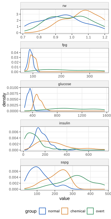
glucose and fpg separate the overt group, sspg separates normal from the two diabetic groups; rw barely differs. Reproduces Holmes and Huber (2019), Figure 12.3. Download: PDF · SVGCellular phenotypes. Neumann et al. (2010) trained a classifier on about 3000 nuclei labelled by an expert and applied it to some \(2\times10^9\) nuclei from genome-wide RNAi time-lapse movies, assigning each to one of 16 morphology classes (the book's Figure 12.4, images from the paper, not reproduced). Two lessons: classification scales an expert's judgement, and the class frequencies are very unbalanced, so the overall misclassification rate is a poor summary (Section 12.5).
Embryonic cell states. The mouse embryo single-cell arrays of Ohnishi et al. (2014), met in Chapters 3, 5 and 7, return in Sections 12.3.2 and 12.6.3: predicting the embryonic day from four genes, and the genotype from all 45,101 probes.
12.3 Linear discrimination
Before any method, the target. If we knew the joint distribution of \((X,Y)\), what would be the best classifier?
Result 12.1 (the Bayes classifier is optimal) Sections 12.3, 12.5, (12.1)
Under 0-1 loss the rule \(g^*(\x)=\argmax_k p_k(\x)\), with \(p_k(\x)=\pi_kf_k(\x)/\sum_l\pi_lf_l(\x)\) by Bayes' theorem, minimises the misclassification risk \(\MCR(g)=\Pr(g(X)\ne Y)\) over all rules \(g\). Its risk, the Bayes risk, is
\[ R^*=\E\big[1-\max_kp_k(X)\big]. \]For two classes, \(g^*(\x)=1\) exactly when \(p_1(\x)>\tfrac12\), equivalently when the likelihood ratio \(f_1(\x)/f_2(\x)\) exceeds \(\pi_2/\pi_1\).
Proof
Condition on \(X=\x\). For any rule \(g\), \(\Pr(g(X)\)
Every classifier of this chapter estimates \(g^*\) somehow. Generative methods (LDA, QDA) model \(\pi_k\) and \(f_k\) and plug them into Bayes' theorem; discriminative methods (logistic regression, Section 12.6.1) model \(p_k(\x)\) directly; nearest neighbours and kernel methods (Section 12.7) estimate the decision directly.
12.3.1 Diabetes data
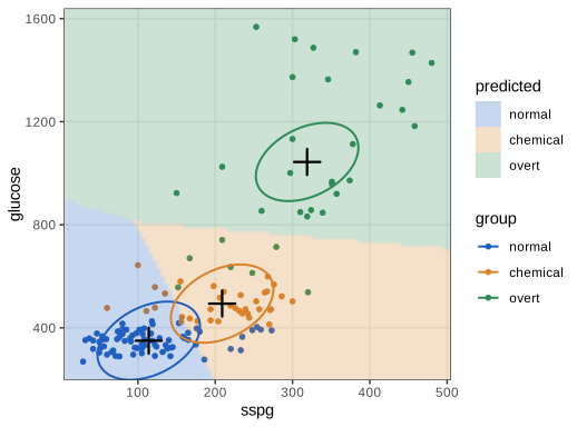
We predict the group from sspg and glucose (Figure 12.5).
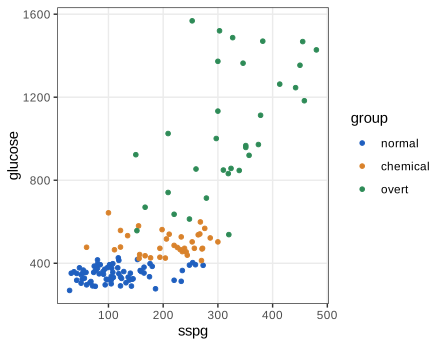
sspg and glucose, coloured by group. Reproduces Holmes and Huber (2019), Figure 12.5. Download: PDF · SVGDefinition 12.2 (Gaussian class models: LDA and QDA) Section 12.3
Assume \(X\given Y=k\sim\N_p(\bm\mu_k,\bm\Sigma_k)\) with priors \(\pi_k\). With \(\bm\Sigma_k=\bm\Sigma\) for all \(k\), the Bayes rule of Result 12.1 becomes "largest linear discriminant"
\[ \delta_k(\x)=\x^\T\bm\Sigma^{-1}\bm\mu_k-\tfrac12\bm\mu_k^\T\bm\Sigma^{-1}\bm\mu_k+\log\pi_k, \]which is linear discriminant analysis (LDA). With class-specific covariances it becomes "largest quadratic discriminant"
\[ \delta_k(\x)=-\tfrac12\log|\bm\Sigma_k|-\tfrac12(\x-\bm\mu_k)^\T\bm\Sigma_k^{-1}(\x-\bm\mu_k)+\log\pi_k, \]which is quadratic discriminant analysis (QDA). In practice the parameters are replaced by the estimates of Filling the gap 12.1.
Derivation
\(\log(\pi_kf_k(\x))\)
Filling the gap 12.1: the estimates that lda plugs in Section 12.3.1
The book calls lda without saying what it estimates. The log-likelihood of the Gaussian class model with a shared covariance, for labelled data, is
and its maximisers are the class fractions \(\hat\pi_k=n_k/n\), the class means \(\hat{\bm\mu}_k=\bar\x_k\), and the pooled within-class covariance \(\hat{\bm\Sigma}\)
Derivation
Priors. \(\sum_i\log\pi_{y_i}=\sum_kn_k\log\pi_k\) under \(\sum_k\pi_k=1\); the Lagrangian \(\sum_kn_k\log\pi_k-\nu(\sum_k\pi_k-1)\) gives \(n_k/\pi_k=\nu\), so \(\pi_k\propto n_k\), \(\hat\pi_k=n_k/n\); it is the maximum because \(\sum n_k\log\pi_k\) is strictly concave.
Means. For fixed \(\bm\Sigma\), the terms with \(\bm\mu_k\) are \(-\tfrac12\sum_{i:y_i=k}(\x_i\)
Covariance. With \(\mathbf{S}\)
What MASS::lda uses. Its default (method = "moment") replaces the divisor \(n\) by \(n-K\), the unbiased version: each class mean uses up one degree of freedom. The class means do not depend on the prior, and neither does the pooled covariance. Plugging these estimates into the LDA discriminants reproduces the classes and posterior probabilities of MASS::lda on the diabetes data to \(10^{-15}\).
On the two variables, LDA misclassifies 26 of the 145 patients (rate 0.1793), with the same confusion table as the book: 69, 24 and 26 correct in the normal, chemical and overt groups. Figure 12.6 shows the regions, the class centres and one ellipse per class.
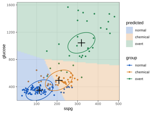
sspg and glucose with the class fractions as priors. The regions are the Bayes rule of the fitted Gaussian model on a 100 × 100 grid; the plus signs are the class means; each ellipse is the set of points at Mahalanobis distance 1 from a class mean under the pooled covariance, so all three have the same size and orientation. Reproduces Holmes and Huber (2019), Figure 12.6. Download: PDF · SVGNote on the text: what the ellipses are
The caption of the book's Figure 12.6 says the ellipses are "contours of equal class membership probability". They are contours of equal class-conditional density: the book builds them as unitcircle %*% solve(scaling), and because the scaling matrix \(\mathbf{S}\) of lda satisfies \(\mathbf{S}^\T\hat{\bm\Sigma}\mathbf{S}=\mathbf{I}\) (checked to \(10^{-16}\)), a row \(\mathbf{u}^\T\mathbf{S}^{-1}\) with \(\|\mathbf{u}\|=1\) has \(\mathbf{u}^\T\mathbf{S}^{-1}\hat{\bm\Sigma}^{-1}\mathbf{S}^{-\T}\mathbf{u}\)
Result 12.2 (LDA boundaries are hyperplanes; how the prior moves them) Questions 12.2, 12.4, 12.7
The LDA boundary between classes \(k\) and \(l\) is the hyperplane
\[ \mathbf{a}_{kl}^\T\x=c_{kl},\qquad \mathbf{a}_{kl}=\bm\Sigma^{-1}(\bm\mu_k-\bm\mu_l),\quad c_{kl}=\tfrac12(\bm\mu_k+\bm\mu_l)^\T\bm\Sigma^{-1}(\bm\mu_k-\bm\mu_l)-\log\frac{\pi_k}{\pi_l}. \](a) Its normal \(\mathbf{a}_{kl}\) is parallel to \(\bm\mu_k-\bm\mu_l\) only if \(\bm\mu_k-\bm\mu_l\) is an eigenvector of \(\bm\Sigma\) (for instance if \(\bm\Sigma\propto\mathbf{I}\)). (b) With equal priors it passes through the midpoint \((\bm\mu_k+\bm\mu_l)/2\). (c) Changing the priors translates it, without rotating it, by \(\log(\pi_k/\pi_l)/\Delta_{kl}\) in Mahalanobis units away from class \(k\), where \(\Delta_{kl}^2\)
Proof
\(\delta_k(\x)-\delta_l(\x)\)
On the diabetes data, the angle between \(\hat{\mathbf{a}}\) and \(\hat{\bm\mu}_\text{normal}-\hat{\bm\mu}_\text{chemical}\) is 46.9°, and points on the explicit line have equal discriminants for normal and chemical to \(10^{-15}\).
Questions 12.1–12.5 Section 12.3.1
12.1 (the printout of lda). "Prior probabilities" are \(\hat\pi_k=n_k/n\) (0.524, 0.248, 0.228); "Group means" are \(\bar\x_k\); "Coefficients of linear discriminants" and "Proportion of trace" are explained in Filling the gap 12.2.
12.2. The chemical-overt boundary is not perpendicular to the line joining the centres because the pooled covariance is not a multiple of the identity (Result 12.2(a)): the boundary is conjugate to the mean difference with respect to \(\hat{\bm\Sigma}\), which is why it is tangent to the tilted ellipses in the direction the book describes.
12.3. Far from all centres the posterior probabilities of the Gaussian model are still near 0 or 1 (they depend only on differences of discriminants, which grow linearly), so the model is overconfident exactly where it has no data. A sensible confidence measure there is the density \(\sum_k\hat\pi_k\hat f_k(\x)\) or the Mahalanobis distance to the nearest centre, not the posterior.
12.4. The normal-chemical boundary is shifted towards the chemical group because \(\hat\pi_\text{normal}\)
12.5. The coloured regions can be drawn for any classifier, even a black box, because they only need predictions on a grid; the centres and ellipses are specific to the Gaussian model.
Filling the gap 12.2: discriminant coordinates, "proportion of trace", and why two coordinates suffice Question 12.1, Figure 12.9
lda also returns Fisher's discriminant coordinates. Let \(\hat{\bm\Sigma}\) be the pooled within-class covariance and \(\mathbf{B}\)
Result 12.3 (the discriminant coordinates carry all the information)
If \(\hat{\bm\Sigma}\) has full rank, the LDA classification of \(\x\) depends on \(\x\) only through its \(r=\min(K-1,p)\) discriminant coordinates \(\mathbf{z}=\mathbf{S}^\T(\x-\bar\x)\): it assigns \(\x\) to the class minimising \(\tfrac12\|\mathbf{z}-\mathbf{m}_k\|^2-\log\pi_k\), where \(\mathbf{m}_k=\mathbf{S}^\T(\bar\x_k-\bar\x)\).
Proof
Let \(\mathbf{A}\) be any \(p\times p\) matrix with \(\mathbf{A}^\T\hat{\bm\Sigma}\mathbf{A}=\mathbf{I}\) (a full sphering); then \(\hat{\bm\Sigma}^{-1}=\mathbf{A}\mathbf{A}^\T\) and, with \(\tilde{\x}=\mathbf{A}^\T(\x-\bar\x)\) and \(\tilde{\mathbf{m}}_k=\mathbf{A}^\T(\bar\x_k-\bar\x)\), the Mahalanobis distance is \((\x-\bar\x_k)^\T\hat{\bm\Sigma}^{-1}(\x-\bar\x_k)\)
The R code uses this to draw the exact LDA regions in the discriminant plane (Figure 12.9). The book instead fits a second LDA to the projected points with the predicted classes as labels, which only approximates the regions. MASS::lda computes \(\mathbf{S}\) by a singular value decomposition that drops directions with singular value below \(10^{-4}\); the course code writes these steps out (lda_mass) and they reproduce MASS::lda to \(10^{-14}\), also when \(p>n\).
Questions 12.6 and 12.7 Section 12.3.1
12.6 (all five variables). The training error falls from 26 to 14 of 145 (0.0966), with the book's table. The honest leave-one-out errors (Section 12.4.1) are 26/145 = 0.179 for two variables and 16/145 = 0.110 for five: the gain is real but smaller than the training error suggests. QDA on the same two variables does much better (7 training errors, 9 leave-one-out errors): the overt group is far more spread out than the others, so a shared covariance is a poor model here.
12.7 (explicit lines). The separating lines are \(\hat{\mathbf{a}}_{kl}^\T\x=\hat c_{kl}\) of Result 12.2 with the plug-in estimates; in the plane \(x_2=(\hat c_{kl}-\hat a_{kl,1}x_1)/\hat a_{kl,2}\). Each line is drawn only where its two classes beat the third.
12.3.2 Predicting embryonic cell state from gene expression
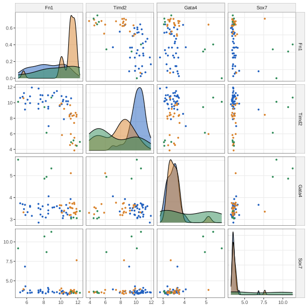
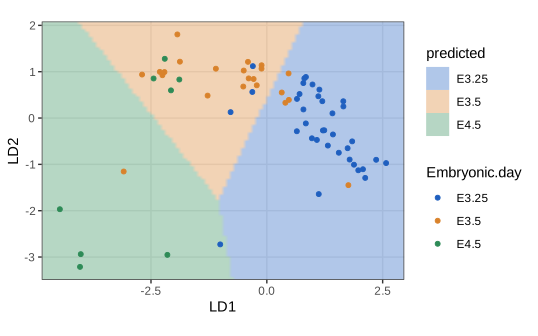
We now predict the embryonic day (E3.25, E3.5, E4.5) of the 66 wild-type cells from the probes for Fn1, Timd2, Gata4 and Sox7 (Figure 12.8). The scaling matrix rounds to the book's values (LD1: \(-0.2, 0.5, -0.1, -0.7\); LD2: \(0.4, 0.0, 0.6, -0.5\)); the training error of LDA is 14 of 66 (0.212).
Filling the gap 12.3: QDA, the number of parameters, and why both methods fail with 1000 genes Questions 12.8, 12.9
Counting parameters. LDA estimates \(K-1\) free priors, \(Kp\) means and one symmetric covariance, \(p(p+1)/2\) entries; QDA estimates \(K\) covariances, \(Kp(p+1)/2\) entries. For \(K=3\), \(p=4\): 24 against 44. For \(p=1000\): about 0.5 million against 1.5 million, from 101 cells.
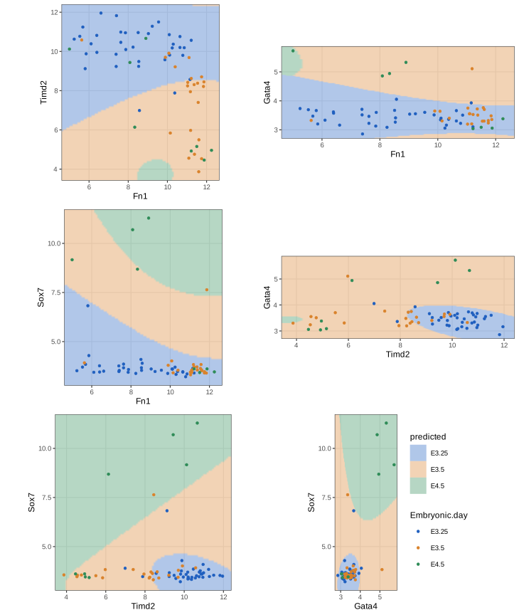
QDA estimates. The maximum likelihood estimates are \(\hat\pi_k=n_k/n\), \(\bar\x_k\) and \(\hat{\bm\Sigma}_k\)MASS::qda uses divisor \(n_k-1\). The boundary \(\{\delta_k=\delta_l\}\) is the zero set of a quadratic polynomial in \(\x\): a conic in the plane (ellipse, parabola, hyperbola or a pair of lines), as Figure 12.10 shows.
Why the high-dimensional fits break down
The sample covariance of class \(k\) is \(\frac1{n_k-1}\mathbf{R}_k^\T\mathbf{R}_k\), where \(\mathbf{R}_k\) is the \(n_k\times p\) matrix of centred rows. The rows of \(\mathbf{R}_k\) sum to zero, so \(\operatorname{rank}\mathbf{R}_k\le n_k-1\), and \(\hat{\bm\Sigma}_k\) is singular whenever \(p\ge n_k\): its inverse and \(\log|\hat{\bm\Sigma}_k|\) do not exist. qda checks this and stops with "some group is too small for 'qda'" (the message the R code records). The pooled covariance has rank at most \(n-K\); with 101 arrays and 1000 genes it is singular too. lda does not stop: its singular value decomposition keeps only the directions with non-negligible within-class variance and warns that "variables are collinear". The fitted rule then lives in a random-looking subspace of dimension at most \(n-K\), which is the mechanism behind Section 12.4.
12.4 Machine learning vs rote learning
A rule that memorises the training data has zero training error and no value. The book makes the point with LDA on pure noise: \(n=20\) objects, \(p\) standard normal features, and labels "apple" or "orange" from fair coin flips, so that no rule can do better than error \(1/2\) on new data. Figure 12.11 averages the training error over 100 such data sets.
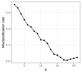
Why can a linear rule fit coin flips? Because in enough dimensions almost every labelling is linearly separable.
Result 12.4 (counting linearly separable labellings)
Call \(n\) points in \(\R^d\) in general position if every subset of at most \(d\) of them is linearly independent. The number of labellings \(y\in\{-1,+1\}^n\) that can be realised as \(y_i=\sgn(\w^\T\x_i)\) by some \(\w\) (a hyperplane through the origin) is
\[ C(n,d)=2\sum_{k=0}^{d-1}\binom{n-1}{k}. \]For affine hyperplanes \(\w^\T\x+b\) in \(\R^p\), apply this to the points \((\x_i,1)\in\R^{p+1}\), so \(d=p+1\). Hence if \(n\) points in general position in \(\R^p\) receive independent fair labels, the probability that the labels are linearly separable is
\[ \Pr(\text{separable})=\frac{C(n,p+1)}{2^n}=\Pr\big(\Bin(n-1,\tfrac12)\le p\big). \]Proof
Boundary values. One point (\(\x_1\ne\mathbf{0}\)) has both labellings, \(C(1,d)=2\). In \(d=1\) the points are non-zero numbers and \(\sgn(wx_i)\) has exactly two patterns (\(w>0\), \(w<0\)): \(C(n,1)=2\). Both agree with the formula.
Recursion \(C(n+1,d)=C(n,d)+C(n,d-1)\). Take a labelling of \(\x_1,\dots,\x_n\) that is realised by some \(\w\). Since general position is an open condition we may perturb \(\w\) so that \(\w^\T\x_{n+1}\ne0\); the labelling therefore extends in at least one way to \(\x_{n+1}\). It extends in both ways if and only if it is realised by some \(\w\) with \(\w^\T\x_{n+1}=0\). Indeed, if \(\w_1,\w_2\) realise the two extensions, then \(\w_1^\T\x_{n+1}>0>\w_2^\T\x_{n+1}\), and a convex combination \(\w=t\w_1+(1-t)\w_2\) has \(\w^\T\x_{n+1}=0\) while still giving every \(\x_i\), \(i\le n\), the common sign of \(\w_1^\T\x_i\) and \(\w_2^\T\x_i\). Conversely, if \(\w^\T\x_{n+1}=0\) and \(\w\) realises the labelling, then \(\w\pm\varepsilon\x_{n+1}\) for small \(\varepsilon>0\) realise it too and put \(\x_{n+1}\) on either side. The vectors \(\w\perp\x_{n+1}\) form a \((d-1)\)-dimensional space, and \(\w^\T\x_i=\w^\T\mathbf{q}_i\) where \(\mathbf{q}_i\) is the projection of \(\x_i\) onto that space; the projected points are in general position in \(\R^{d-1}\), so exactly \(C(n,d-1)\) labellings extend both ways. Counting: \(C(n+1,d)\)
Solution. By induction on \(n\): if \(C(n,d)=2\sum_{k<d}\binom{n-1}{k}\) for all \(d\), then \(C(n,d)+C(n,d-1)\)
We count, by linear programming, the separable labellings of 8 random points in the plane: 58, which is \(C(8,3)=2(1+7+21)\).
For \(n=20\) the probability that random labels are separable is 0.032 with \(p=5\) features, exactly \(1/2\) with \(p=9\), 0.968 with \(p=13\) and 0.9978 with \(p=15\). LDA does not search for a separating hyperplane, but with this much freedom its fitted direction separates the training points too, which is the steady fall in Figure 12.11.
Note on the text: the upturn beyond \(p=18\)
The book attributes the slight rise of the training error for the largest \(p\) to "numerical properties of the lda implementation". There is a structural reason. The pooled within-class scatter of 20 points in 2 classes has rank at most \(n-K=18\) (Filling the gap 12.3). For \(p\le18\) LDA uses all directions; for \(p>18\) lda discards the null directions of the within-class scatter and fits within an 18-dimensional subspace that the data choose, so extra features no longer add freedom and the fit to random labels gets slightly worse. The minimum of Figure 12.11 sits exactly at \(p=n-K=18\).
Question 12.10 (the replicate loop)
Each point of Figure 12.11 is an average over 100 data sets. One data set gives a noisy estimate of the expected training error (its standard deviation is roughly \(\sqrt{e(1-e)/n}\) with \(e\) the error, about 0.1 at \(p=2\)); averaging 100 independent replicates divides that by 10. This is possible only because the data are simulated.
How optimistic is the training error in general? For regression with squared loss there is an exact answer.
Result 12.5 (optimism of the training error)
Let \(y_i=\mu_i+\varepsilon_i\) with fixed \(\x_i\), independent errors of variance \(\sigma^2\), and fitted values \(\hat y_i\). Let \(y_i^0\) be a new response at the same \(\x_i\), independent of the training data, and \(\Err_\text{in}=\frac1n\sum_i\E(y_i^0-\hat y_i)^2\). Then
\[ \E\big[\Err_\text{in}\big]-\E\big[\err\big]=\frac2n\sum_{i=1}^n\cov(\hat y_i,y_i), \]which for a linear smoother \(\hat\y=\mathbf{H}\y\) equals \(2\sigma^2\Tr(\mathbf{H})/n\), and for least squares with \(p\) coefficients \(2\sigma^2p/n\).
Proof
Write \(\hat y_i-\mu_i=e_i\). Since \(y_i^0\) is independent of \(\hat y_i\), \(\E(y_i^0-\hat y_i)^2=\sigma^2+\E e_i^2\). For the training response, \(\E(y_i-\hat y_i)^2\)
We confirm \(2\sigma^2p/n=0.267\) for \(n=30\), \(p=4\) by simulation (0.268). The more a fitted value follows its own observation, the more optimistic the training error; this is the general content of the word "overfitting".
12.4.1 Cross-validation
Definition 12.3 (\(K\)-fold and leave-one-out cross-validation) Section 12.4.1
Split \(\{1,\dots,n\}\) into \(K\) folds \(F_1,\dots,F_K\). For each \(k\), fit the rule \(\hat f^{(-k)}\) on the data outside \(F_k\) and evaluate it on \(F_k\). The cross-validation estimate is
\[ \CV_K=\frac1n\sum_{k=1}^K\sum_{i\in F_k}L\big(y_i,\hat f^{(-k)}(\x_i)\big). \]Leave-one-out (LOO) is \(K=n\): each observation is predicted by the rule fitted to the other \(n-1\).
Result 12.6 (what cross-validation estimates)
If the observations are independent and identically distributed, then exactly
\[ \E\big[\CV_\text{LOO}\big]=\Err_{n-1},\qquad \E\big[\CV_K\big]=\Err_{n-n/K}\ \ (\text{equal folds}), \]where \(\Err_m\) is the expected test error of the procedure trained on \(m\) observations (Definition 12.1). Leave-one-out is therefore unbiased for a training size one less than ours; since learning curves \(\Err_m\) decrease and flatten as \(m\) grows, its bias \(\Err_{n-1}-\Err_n\) is small. \(K\)-fold CV estimates the error at training size \(n(1-1/K)\) and is pessimistic, more so for small \(K\) and steep learning curves.
Proof
Fix \(i\). The rule \(\hat f^{(-i)}\) is a function of \(D^{(-i)}\), a sample of \(n-1\) independent draws from \(P\), and \((\x_i,y_i)\) is a further independent draw. Conditioning on \(D^{(-i)}\), \(\E[L(y_i,\hat f^{(-i)}(\x_i))\given D^{(-i)}]\)
Unbiasedness says nothing about variance. The \(n\) LOO training sets overlap in \(n-2\) points, so the \(n\) terms are strongly correlated and LOO can be quite variable; the book's remark that the LOO training sets are "all very similar" is this. Five- or ten-fold CV is a common compromise. We simulate a one-dimensional nearest-centroid classifier with \(n=20\): mean LOO error 0.2318, mean error of the rules trained on 19 points 0.2324, on 20 points 0.2321.
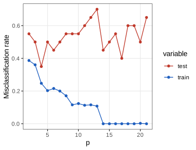
Question 12.11 (why Figure 12.12 is wiggly)
It uses one data set, so each point is a single LOO estimate whose standard deviation is at least \(\sqrt{0.25/20}\approx0.11\) (more, because of the correlation between the terms). Averaging over replicate data sets, as in Figure 12.11, removes the wiggles; the cross-validation demonstration does this when "simulate" is chosen.
Result 12.7 (leave-one-out without refitting, for linear smoothers)
For least squares with hat matrix \(\mathbf{H}=\X(\X^\T\X)^{-1}\X^\T\), leverages \(h_{ii}\) and fitted values \(\hat y_i\), the leave-one-out prediction error is
\[ y_i-\hat y_i^{(-i)}=\frac{y_i-\hat y_i}{1-h_{ii}},\qquad \CV_\text{LOO}=\frac1n\sum_{i=1}^n\Big(\frac{y_i-\hat y_i}{1-h_{ii}}\Big)^2. \]Proof
Let \(\mathbf{A}=\X^\T\X\). Removing row \(i\) gives \(\mathbf{A}-\x_i\x_i^\T\) and \(\X^\T\y-\x_iy_i\). By the Sherman-Morrison formula, \((\mathbf{A}-\x_i\x_i^\T)^{-1}\)
and \(y_i-\hat y_i^{(-i)}\)MASS::lda(CV = TRUE) uses an analogous rank-one downdate of the pooled covariance.
Filling the gap 12.4: every data-driven step belongs inside the loop Sections 12.4.1, 12.6.2, Question 12.23
The book warns that tuning \(\lambda\) by CV and then quoting the CV error is optimistic, and cites Ambroise and McLachlan (2002). The cleanest case is feature selection. Suppose we rank all features by a two-sample \(t\)-statistic on the full data, keep the top \(k\), and then cross-validate a classifier on those \(k\). Result 12.6 needs the held-out point to be independent of the fitted rule; here the rule depends on the held-out labels through the selection step, so the argument fails. The selected features are those on which, by chance, the held-out samples agree with their labels, and they look predictive in every fold.
The R code makes this concrete with pure noise: \(n=40\) samples (20 per class), 500 standard normal features, the top \(k=10\) by \(|t|\), LDA, leave-one-out. Over 50 data sets the mean CV error is 0.163 when the features are selected once on all data, and 0.532 when they are reselected inside each fold; the true error of any rule is 0.5. Selection inside the loop is Algorithm 12.1.
Algorithm 12.1 (cross-validation of a pipeline with feature selection)
- Split the samples into folds \(F_1,\dots,F_K\) (for LOO, \(K=n\)).
- For each \(k\): using only the samples outside \(F_k\), compute the feature scores, select the features, choose transformations, normalisations and tuning parameters, and fit the classifier.
- Apply the resulting pipeline unchanged to the samples in \(F_k\) and record their losses.
- Report the average loss. The selected feature set may differ between folds; the estimate refers to the procedure, not to one feature set.
12.4.2 The curse of dimensionality
Now give the classes a real difference: in each of 100 data sets with \(n=20\) and 20 features, the first six features have mean 1 for apples and 2 for oranges, the rest are noise. Figure 12.13 shows the LOO error first falling (useful features are added) and then rising (noise features are added).
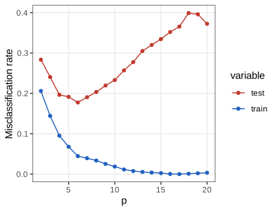
Result 12.8 (the best possible error, and the price of noise features)
(a) Two classes with equal priors and \(X\given Y=k\sim\N(\bm\mu_k,\mathbf{I})\) have Bayes error \(\Phi(-\Delta/2)\), where \(\Delta=\|\bm\mu_1-\bm\mu_2\|\). In the book's example, using the first \(p\) features gives \(\Delta=\sqrt{\min(p,6)}\): Bayes error 0.240 for \(p=2\), 0.110 for \(p\ge6\). Extra noise features cannot lower and do not raise the Bayes error.
(b) The estimated rule pays for every feature. For the nearest-centroid rule (LDA with the covariance known to be \(\mathbf{I}\)), with \(n/2\) training points per class and \(p\) features of which the informative ones give separation \(\Delta\), the test error satisfies, for large \(p\) and \(n\),
\[ \Err\approx\Phi\Big(-\frac{\Delta^2}{2\sqrt{\Delta^2+4p/n}}\Big), \]which tends to \(1/2\) as \(p/n\to\infty\) with \(\Delta\) fixed. Estimating the covariance as well, as LDA does, adds a further penalty that grows as \(p\) approaches \(n-2\).
Proof
(a) By Result 12.1 the Bayes rule compares the two Gaussian densities; with identity covariance it assigns \(\x\) to the nearer mean, i.e. thresholds \(T\)
(b) Let \(\hat{\bm\mu}_k=\bm\mu_k+\mathbf{e}_k\) with independent \(\mathbf{e}_k\sim\N(\mathbf{0},\frac2n\mathbf{I})\), \(\hat{\mathbf{d}}=\hat{\bm\mu}_1-\hat{\bm\mu}_2\) and \(\mathbf{c}=(\hat{\bm\mu}_1+\hat{\bm\mu}_2)/2\). Conditionally on the training data the rule "class 1 if \(\hat{\mathbf{d}}^\T(\x-\mathbf{c})>0\)" errs on a class-1 point with probability \(\Phi\big(-\hat{\mathbf{d}}^\T(\bm\mu_1\)
The middle terms have mean 0 and variance \(O(\Delta^2/n)\); \(\|\mathbf{e}_1\|^2-\|\mathbf{e}_2\|^2\) has mean 0 and variance \(O(p/n^2)\). So the numerator is \(\tfrac12\Delta^2+o_P(1)\) as \(n\to\infty\) with \(p/n\) bounded. In the denominator, \(\|\hat{\mathbf{d}}\|^2\)
A simulation with \(p=n=200\), \(\Delta^2=4\) gives 0.241 against the approximation 0.240 (Bayes error 0.159). In the book's setting (\(n=20\), \(\Delta^2=6\)) the formula gives 0.132 at \(p=6\) and 0.171 at \(p=20\); LDA, which also estimates the covariance, reaches 0.178 and 0.372.
Bellman (1961) coined the name for the related fact that high-dimensional spaces cannot be sampled densely: a grid of spacing 0.1 needs \(10^p\) points, \(10^{100}\) in 100 dimensions. The book's Questions 12.12 to 12.14 make three consequences quantitative.
Result 12.9 (three facts about the unit cube \([0,1]^p\)) Questions 12.12–12.14
(a) Neighbourhoods are not local. With \(N\) uniform points, a sub-cube expected to contain \(k\) of them has side \((k/N)^{1/p}\): \(10^{-5}\) for \(p=1\) but 0.75 for \(p=40\) and 0.97 for \(p=400\) when \(N=10^6\), \(k=10\).
(b) Almost everything is near the boundary. The fraction of the volume within \(\varepsilon\) of the surface is \(1-(1-2\varepsilon)^p\): for \(\varepsilon=0.01\), 2% in one dimension, 64% for \(p=50\), 99.97% for \(p=400\).
(c) Distances concentrate. For independent uniform \(U,V\in[0,1]^p\) and \(D=\|U-V\|\), \(\E D^2=p/6\), \(\var D^2=7p/180\), and the coefficient of variation of \(D\) satisfies \(\sqrt p\cdot\mathrm{sd}(D)/\E D\)
Proof
(a) A sub-cube of side \(s\) has volume \(s^p\) and contains on average \(Ns^p\) points; set \(Ns^p=k\). (b) The points at distance at least \(\varepsilon\) from every face form the cube \([\varepsilon,1-\varepsilon]^p\) of volume \((1-2\varepsilon)^p\). (c) \(D^2=\sum_{j=1}^pW_j\) with \(W_j=(U_j-V_j)^2\) independent. \(U_j-V_j\) has the triangular density \(1-|t|\) on \([-1,1]\), so \(\E W_j\)
Simulation: \(\E D^2=1.669\), \(\var D^2=0.390\) for \(p=10\) (theory 1.667, 0.389); for \(p=10^4\) the simulated CV of Figure 12.17 is 0.00597 against 0.00592. The dashed curve in Figure 12.17 is the approximation; it is already accurate at \(p=10\). This is the "central limit theorem" argument the book alludes to.
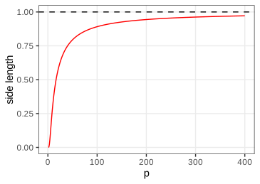
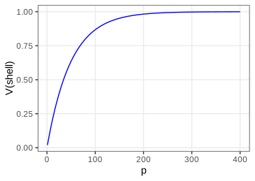
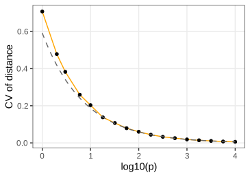
For prediction these facts mean that in high dimension a "local" method such as \(k\)-nearest neighbours averages over neighbours that are not near, most new points require extrapolation, and "nearest" carries little information when all distances are about equal. Methods that work in high dimension do so by assuming structure: linearity, sparsity, or smoothness along few directions.
12.5 Objective functions
The misclassification rate has the population version and the sample version
\[ \MCR=\E\big[\one\{\hat y\ne y\}\big], \tag{12.1} \] \[ \widehat{\MCR}=\frac1n\sum_{i=1}^n\one\{\hat y_i\ne y_i\}. \tag{12.2} \](The HTML edition of the book prints (12.1) twice on one line; it is one formula.) Errors of different kinds can be weighted, and the full picture is the confusion table table(truth, response).
Definition 12.4 (confusion table and derived measures) Section 12.5, Question 12.15, (12.3)
For two classes, call one "positive" (diseased) and count true positives TP, false negatives FN, false positives FP and true negatives TN; P = TP + FN and N = FP + TN are the numbers of actual positives and negatives.
- Sensitivity (true positive rate, recall) \(\mathrm{TPR}=\mathrm{TP}/\mathrm{P}\); specificity (true negative rate) \(\mathrm{SPC}=\mathrm{TN}/\mathrm{N}\).
- Positive predictive value (precision) \(\mathrm{PPV}=\mathrm{TP}/(\mathrm{TP}+\mathrm{FP})\); negative predictive value \(\mathrm{TN}/(\mathrm{TN}+\mathrm{FN})\).
- Jaccard index (12.3) of \(A=\{i:y_i=1\}\) and \(B=\{i:\hat y_i=1\}\): \(J\)
\({}=|A\cap B|/|A\cup B|\) \({}=\mathrm{TP}/(\mathrm{TP}+\mathrm{FP}+\mathrm{FN})\); it ignores TN, which suits rare events. - For a score \(s(\x)\) and threshold \(t\) (call positive if \(s>t\)), the ROC curve is \(t\mapsto(1-\mathrm{SPC}(t),\mathrm{TPR}(t))\), and the AUC is the area under it.
Result 12.11 (misclassification, sensitivity, specificity and prevalence) Questions 12.15, 12.21
The per-class misclassification rates are \(1-\mathrm{TPR}\) (positives called negative) and \(1-\mathrm{SPC}\) (negatives called positive), and with prevalence \(\pi=\Pr(Y=1)\)
\[ \MCR=\pi\,(1-\mathrm{TPR})+(1-\pi)(1-\mathrm{SPC}),\qquad \mathrm{PPV}=\frac{\pi\,\mathrm{TPR}}{\pi\,\mathrm{TPR}+(1-\pi)(1-\mathrm{SPC})}. \]Proof
\(\Pr(\hat Y\)
Note on the text: sensitivity and specificity swapped
The book says that sensitivity "is related to the misclassification of healthy as ill" and specificity to "misclassification of ill as healthy". It is the other way round: by Result 12.11, \(1-\)sensitivity is the rate at which ill (positive) subjects are called healthy, and \(1-\)specificity the rate at which healthy subjects are called ill. The formulas given in the book's answer to Question 12.15 are correct.
Result 12.12 (the AUC is a probability)
Let \(S^+\) and \(S^-\) be the scores of an independent random positive and negative case. Then \(\mathrm{AUC}=\Pr(S^+>S^-)+\tfrac12\Pr(S^+=S^-)\). For a sample, the trapezoidal area under the empirical ROC curve equals the Mann-Whitney statistic \(U/(\mathrm{P}\cdot\mathrm{N})\).
Proof
For continuous scores with survival functions \(\bar F_\pm(t)=\Pr(S^\pm>t)\), the ROC curve is \((\bar F_-(t),\bar F_+(t))\) as \(t\) runs from \(+\infty\) to \(-\infty\), so \(\mathrm{AUC}\)pROC::auc.)
For probabilistic predictions \(\hat p_i=\hat\Pr(Y_i=1\given\x_i)\) the book uses the log loss
\[ \log\text{loss}=-\frac1n\sum_{i=1}^n\big[y_i\log\hat p_i+(1-y_i)\log(1-\hat p_i)\big], \tag{12.4} \]which is minus the average Bernoulli log-likelihood (the binomial deviance of Section 12.6.2 is twice it), and for regression the mean squared error
\[ \widehat{\MSE}=\frac1n\sum_{i=1}^n(\hat Y_i-Y_i)^2. \tag{12.5} \]Each loss has its own optimal prediction:
Result 12.10 (what each loss asks for)
(a) Squared loss: \(\E[(Y-c)^2\given X=\x]\) is minimised by \(c=\E[Y\given X=\x]\), the regression function. (b) Cost-weighted 0-1 loss with cost \(c_\text{FN}\) for a missed positive and \(c_\text{FP}\) for a false alarm: the optimal rule calls positive when \(p_1(\x)>c_\text{FP}/(c_\text{FP}+c_\text{FN})\); equal costs give the Bayes rule. (c) Log loss is proper: if \(Y\given\x\sim\mathrm{Bernoulli}(p)\), the expected loss \(-p\log q-(1-p)\log(1-q)\) is uniquely minimised at \(q=p\). It is infinite when a confident prediction (\(q\in\{0,1\}\)) is wrong.
Proof
(a) \(\E[(Y-c)^2\given\x]\)
A medical test has a threshold that trades sensitivity against specificity; one point of the trade-off is rarely enough, so we report the whole ROC curve (or a precision-recall curve when positives are rare).
12.6 Variance-bias trade-off
The book's Figure 12.18 (two bull's-eye targets, a schematic not reproduced) separates being systematically off target (bias) from scattering around the target (variance). The book writes the decomposition as
\[ \MSE=\underbrace{\var(\hat Y)}_{\text{variance}}+\underbrace{\E[\hat Y-Y]^2}_{\text{bias}}. \tag{12.6} \]Note on the text: the form of (12.6)
As printed, the second term reads as \(\E[(\hat Y-Y)^2]\), which is the MSE itself. What is meant is the squared bias \((\E\hat Y-Y)^2\), with \(Y\) a fixed target (an estimand). When the target is a new random response, as in prediction, a third term appears: the irreducible noise \(\sigma^2\) (Result 12.13).
Result 12.13 (bias-variance decomposition)
(a) For an estimator \(\hat\theta\) of a fixed \(\theta\): \(\E(\hat\theta-\theta)^2\)
(b) For prediction at a fixed \(\x_0\), with \(Y_0=f(\x_0)+\varepsilon_0\), \(\E\varepsilon_0=0\), \(\var\varepsilon_0=\sigma^2\), and \(\varepsilon_0\) independent of the training data that determine \(\hat f\):
\[ \E\big(Y_0-\hat f(\x_0)\big)^2=\sigma^2+\big(f(\x_0)-\E\hat f(\x_0)\big)^2+\var\hat f(\x_0). \]Proof
(a) Add and subtract \(\E\hat\theta\): \(\E(\hat\theta-\E\hat\theta+\E\hat\theta-\theta)^2\)
We verify (b) for a 7-nearest-neighbour average of \(\sin(2\pi x)\) with \(\sigma=0.3\) at \(x_0=0.25\): simulated 0.1037, decomposition 0.1040.
Why accept bias? Because shrinking can cut variance by more than it adds in squared bias. The simplest example: \(\hat\theta\) unbiased with variance \(v\); the shrunken \(c\hat\theta\) has \(\MSE(c)=c^2v+(1-c)^2\theta^2\), minimised at \(c^*=\theta^2/(\theta^2+v)<1\), and \(\MSE'(1)=2v>0\), so some shrinkage always helps. The catch is that \(c^*\) depends on the unknown \(\theta\); in practice the amount of shrinkage is a tuning parameter chosen from the data, by empirical Bayes (Chapter 8 of the book) or by cross-validation (below).
Result 12.14 (under 0-1 loss, bias can be free) Section 12.6, Friedman (1997)
Two classes, \(f(\x)=\Pr(Y=1\given\x)\), and a classifier that calls 1 when an estimate \(\hat f(\x)>\tfrac12\), with \(\hat f\) independent of the test pair. Then
\[ \Pr(\hat Y\ne Y\given\x)=\min\{f,1-f\}+|2f-1|\cdot\Pr\big(\hat Y\ne g^*(\x)\big). \]If \(\hat f(\x)\) is approximately \(\N(\bar f,s^2)\), then \(\Pr(\hat Y\)
Proof
Suppose \(f>\tfrac12\) (so \(g^*=1\)). Since \(Y\) and \(\hat Y\) are conditionally independent given \(\x\), \(\Pr(\hat Y\)
So a biased \(\hat f\) that is pulled towards \(\tfrac12\) but stays on the correct side costs nothing as long as its variance falls proportionally; under squared loss the same bias would always cost. This is the sense in which "the discreteness of the response absorbs certain biases", and why very simple classifiers (naive Bayes, nearest centroids, heavily penalised models) often classify well while estimating probabilities badly.
12.6.1 Penalization
Penalised versions of LDA exist (Clemmensen et al. 2011; Witten and Tibshirani 2011), but the book switches to logistic regression, the natural home of penalisation. With class \(K\) as reference, the multinomial logistic model is
\[ \log\frac{\Pr(Y=i\given X=\x)}{\Pr(Y=K\given X=\x)}=\beta^0_i+\bb_i^\T\x,\qquad i=1,\dots,K-1. \tag{12.7} \](The book writes \(\beta_i x\); for a single observation \(\x\in\R^p\) the term is the inner product \(\bb_i^\T\x\), and for the data matrix it is \(\X\bb_i\).)
Filling the gap 12.5: the logistic likelihood, its score and Hessian, and when the maximum does not exist (12.7)
Solving (12.7) for the probabilities gives the softmax form \(p_i(\x)=e^{\eta_i}/(1+\sum_{l<K}e^{\eta_l})\) with \(\eta_i=\beta^0_i+\bb_i^\T\x\) and \(\eta_K=0\). The choice of reference is immaterial: replacing \(K\) by \(j\) changes the parameters to \(\beta_i-\beta_j\) (all in the same direction) and leaves every probability unchanged. For two classes, with \(y_i\in\{0,1\}\) and \(\eta_i=\beta^0+\bb^\T\x_i\), the log-likelihood is
\[ \ell(\beta^0,\bb)=\sum_{i=1}^n\big[y_i\eta_i-\log(1+e^{\eta_i})\big]. \]Derivation
\(\log\Pr(Y=y\given\x)\)
Separation. If some \((\beta^0,\bb)\) has \(\eta_i>0\) for all \(y_i=1\) and \(\eta_i<0\) for all \(y_i=0\), then along \(t(\beta^0,\bb)\), \(t\to\infty\), every term \(y_i\eta_i-\log(1+e^{\eta_i})\) increases to 0; but \(\ell<0\) at every finite parameter. The supremum 0 is not attained: the maximum likelihood estimate does not exist. By Result 12.4, this is the typical situation once \(p\ge n-1\), which is one reason the unpenalised model is useless for the microbiome data (\(p=1505\), \(n=114\)). We confirm the score equations and the negative definite Hessian at a glm fit.
Filling the gap 12.6: why logistic regression is "more general" than LDA Section 12.6.1
Under the LDA model (Gaussian classes, shared \(\bm\Sigma\)),
\[ \log\frac{p_i(\x)}{p_K(\x)}=\log\frac{\pi_i}{\pi_K}-\tfrac12(\bm\mu_i+\bm\mu_K)^\T\bm\Sigma^{-1}(\bm\mu_i-\bm\mu_K)+\x^\T\bm\Sigma^{-1}(\bm\mu_i-\bm\mu_K), \]which is exactly of the form (12.7). So LDA and logistic regression fit the same family of posterior probabilities. The difference is in what else is assumed. LDA maximises the full likelihood of \((X,Y)\), and needs the Gaussian model for \(X\) within classes; logistic regression maximises the conditional likelihood of \(Y\) given \(X\) and leaves the distribution of \(X\) free, so it remains valid for skewed, discrete or zero-inflated features such as microbial abundances, and it extends directly to penalties and GLM machinery. When the Gaussian assumption holds, LDA uses more information and is somewhat more efficient. (The derivation is the difference of two LDA discriminants, as in Result 12.2; fitting LDA confirms that its log posterior odds are linear in \(\x\) to \(10^{-14}\).)
When \(p\) is large the maximum likelihood estimates become wildly variable or do not exist. The remedy is to penalise. The book writes
\[ \hat\bb=\argmax_{\bb}\ \ell(\bb,\beta^0;\x)+\lambda\pen(\bb). \tag{12.8} \]Note on the text: the sign in (12.8), the norms, and the elastic-net convention
(1) With a convex penalty and \(\lambda\ge0\), adding \(\lambda\pen(\bb)\) to a quantity being maximised rewards large coefficients. The penalty must be subtracted: \(\hat\bb=\argmax\{\ell-\lambda\pen(\bb)\}\), equivalently \(\argmin\{-\ell+\lambda\pen(\bb)\}\). (2) The book defines \(|\bb|^\nu=\sum_i\beta_i^\nu\); the absolute values are needed, \(\sum_i|\beta_i|^\nu\), which is the \(\nu\)-th power of the \(L_\nu\) norm (for \(\nu=1\), \(\sum_i\beta_i\) is not a norm at all). (3) The book's elastic net \((1-\alpha)|\bb|^1+\alpha|\bb|^2\) makes \(\alpha=0\) the lasso; glmnet, used throughout the chapter, has the opposite convention, \(\frac{1-\alpha}2\|\bb\|_2^2+\alpha\|\bb\|_1\), so its default alpha = 1 is the lasso. These notes use the glmnet convention (Definition 12.5).
Definition 12.5 (ridge, lasso and elastic net, as fitted by glmnet) (12.8)
With the features standardised (mean 0, \(\frac1n\sum_ix_{ij}^2=1\)) and the intercept unpenalised, the penalised logistic regression solves
\[ \min_{\beta^0,\bb}\ -\frac1n\ell(\beta^0,\bb)+\lambda\sum_{j=1}^p\Big[\frac{1-\alpha}2\beta_j^2+\alpha|\beta_j|\Big], \]with \(\alpha=0\) ridge, \(\alpha=1\) lasso, \(0<\alpha<1\) elastic net. For regression, \(-\frac1n\ell\) is replaced by \(\frac1{2n}\|\y-\beta^0-\X\bb\|^2\). Coefficients are reported on the original scale (divided by the feature standard deviations).
Result 12.15 (ridge regression: closed form, shrinkage, and why it beats least squares)
For centred \(\y\) and \(\X\), the minimiser of \(\|\y-\X\bb\|^2+\lambda\|\bb\|^2\), \(\lambda>0\), is unique and equals
\[ \hat\bb_\lambda=(\X^\T\X+\lambda\mathbf{I})^{-1}\X^\T\y=\sum_{j}\frac{d_j}{d_j^2+\lambda}\,\mathbf{v}_j\mathbf{u}_j^\T\y, \]where \(\X=\mathbf{U}\mathbf{D}\mathbf{V}^\T\) is the singular value decomposition; it exists even when \(p>n\). The fit shrinks the least-squares coordinates along \(\mathbf{u}_j\) by \(d_j^2/(d_j^2+\lambda)\), most along directions of small variance, and has effective degrees of freedom \(\Tr\mathbf{H}_\lambda=\sum_jd_j^2/(d_j^2+\lambda)\). If \(\y=\X\bb+\bm\varepsilon\) with \(\var\bm\varepsilon=\sigma^2\mathbf{I}\) and \(\X\) of full column rank, then the total mean squared error \(M(\lambda)=\E\|\hat\bb_\lambda-\bb\|^2\) satisfies
\[ M'(0)=-2\sigma^2\sum_jd_j^{-4}<0,\qquad M(\lambda)<M(0)\ \text{for all}\ 0<\lambda<\sigma^2/\max_j\gamma_j^2, \]where \(\bm\gamma=\mathbf{V}^\T\bb\): some ridge estimator always beats least squares.
Proof
The objective has gradient \(-2\X^\T(\y-\X\bb)+2\lambda\bb\) and Hessian \(2(\X^\T\X+\lambda\mathbf{I})\succ0\), so it is strictly convex and the unique minimiser solves \((\X^\T\X+\lambda\mathbf{I})\bb=\X^\T\y\). With \(\X^\T\X=\mathbf{V}\mathbf{D}^2\mathbf{V}^\T\) and \(\X^\T\y=\mathbf{V}\mathbf{D}\mathbf{U}^\T\y\), the solution is \(\mathbf{V}(\mathbf{D}^2\)
MSE. In the rotated coordinates \(\hat\gamma_{\lambda,j}\)
(Differentiate: \(\frac{\d}{\d\lambda}\frac{d^2}{(d^2+\lambda)^2}\)
We compare the closed form with a numerical minimiser (\(10^{-8}\)), the SVD form, the degrees of freedom, and \(M'(0)\) with a finite difference of the exact matrix formula for \(M\).
Result 12.16 (orthonormal design: proportional shrinkage, soft- and hard-thresholding)
Let \(\X^\T\X=n\mathbf{I}\) and \(z_j=\x_j^\T\y/n\) (the least-squares coefficients). The minimiser of \(\frac1{2n}\|\y\)
Ridge (\(\alpha=0\)) gives \(z_j/(1+\lambda)\), never exactly zero; the lasso (\(\alpha=1\)) gives the soft-threshold \(\Sop(z_j,\lambda)\), exactly zero for \(|z_j|\le\lambda\). For comparison, the best-subset penalty \(\lambda\,\#\{j:\beta_j\ne0\}\) gives the hard threshold \(z_j\one\{|z_j|>\sqrt{2\lambda}\}\).
Proof
Expand: \(\frac1{2n}\|\y-\X\bb\|^2\)
We build an orthonormal design with \(\X^\T\X=64\,\mathbf{I}\) and confirm that glmnet returns exactly these values (\(10^{-16}\)) for \(\alpha=1\) and \(\alpha=0.5\).
Filling the gap 12.7: why the lasso selects, what the penalty means, and what the elastic net adds
Geometry. For convex problems the penalised form and the constrained form \(\min-\ell\) subject to \(\pen(\bb)\le t\) have the same solutions (for each \(\lambda\) there is a \(t\) and conversely, by Lagrangian duality). The \(L_1\) ball \(\{\sum|\beta_j|\le t\}\) has corners on the axes; the elliptical contours of the loss typically first touch it at a corner, where some coordinates are 0. The \(L_2\) ball is round and has no preferred points. The analytic version of the same fact is the kink of \(|\beta|\) at 0 in Result 12.16.
Bayesian reading. Minimising \(-\ell+n\lambda\frac12\|\bb\|^2\) is finding the posterior mode under independent \(\N(0,1/(n\lambda))\) priors on the \(\beta_j\); the lasso is the posterior mode under Laplace (double exponential) priors with rate \(n\lambda\). The penalty is a prior belief that most effects are small, or (lasso) that many are zero.
Grouping. If two features are identical, \(\x_j=\x_k\), the lasso cannot tell them apart: any split of a coefficient between them gives the same fit and the same \(|\beta_j|+|\beta_k|\) when the signs agree, so the solution is not unique and in practice one of the two is picked arbitrarily. With \(\alpha<1\) the solution has \(\hat\beta_j=\hat\beta_k\): replacing both by their average leaves the fit unchanged, does not increase \(|\beta_j|+|\beta_k|\) (triangle inequality), and strictly decreases \(\beta_j^2+\beta_k^2\) unless they are equal (strict convexity of the square). For correlated taxa, as in microbiome data, the elastic net therefore tends to keep groups together.
Result 12.17 (optimality conditions and the start of the path)
With standardised features and fitted probabilities \(p_i\), \((\hat\beta^0,\hat\bb)\) minimises the objective of Definition 12.5 if and only if \(\sum_i(y_i-p_i)=0\) and, for every \(j\),
\[ \frac1n\x_j^\T(\y-\mathbf{p})=\lambda(1-\alpha)\hat\beta_j+\lambda\alpha s_j,\qquad s_j=\sgn\hat\beta_j\ \text{if}\ \hat\beta_j\ne0,\quad s_j\in[-1,1]\ \text{if}\ \hat\beta_j=0. \]In particular \(\hat\bb=\mathbf{0}\) (with \(p_i=\bar y\)) exactly when \(\lambda\ge\lambda_{\max}\), where
\[ \lambda_{\max}=\frac{\max_j|\x_j^\T(\y-\bar y\one)|}{n\,\alpha}. \]Proof
The objective is convex (a convex negative log-likelihood plus a convex penalty), so a point is a minimiser iff zero belongs to its subdifferential. The gradient of \(-\frac1n\ell\) with respect to \(\beta^0\) and \(\beta_j\) is \(-\frac1n\sum_i(y_i-p_i)\) and \(-\frac1n\x_j^\T(\y-\mathbf{p})\) (Filling the gap 12.5), and the subdifferential of the penalty term in \(\beta_j\) is \(\lambda(1\)
This is how glmnet starts its path: we confirm that its first \(\lambda\) equals this \(\lambda_{\max}\) on the microbiome data (0.15005 for the species data of the demonstration), and that the conditions hold at a fitted point (35 active coefficients with \(|\x_j^\T(\y-\mathbf{p})|/n=\lambda\), all others below). For ridge (\(\alpha=0\)) the formula would give \(\infty\); glmnet uses \(\alpha=0.001\) in its place.
Algorithm 12.2 (the regularisation path by coordinate descent)
- Standardise the features. Set \(\lambda_1=\lambda_{\max}\) (Result 12.17) and \(\lambda_m=\lambda_{\max}\,r^{(m-1)/99}\), \(m=1,\dots,100\), with \(r=0.01\) if \(n<p\) and \(10^{-4}\) otherwise. Start from \(\bb=\mathbf{0}\), \(\beta^0=\log\frac{\bar y}{1-\bar y}\).
- For each \(\lambda_m\) in turn, starting from the solution at \(\lambda_{m-1}\) (warm start), repeat until the coefficients stop changing:
- Quadratic approximation. Compute \(p_i\), weights \(w_i=p_i(1-p_i)\) and working residuals \(r_i=(y_i-p_i)/w_i\) at the current fit; this replaces \(-\frac1n\ell\) by the weighted least-squares criterion \(\frac1{2n}\sum_iw_i(z_i-\beta^0-\x_i^\T\bb)^2\) with \(z_i=\eta_i+r_i\) (one Newton step, as in IRLS).
- Coordinate descent on that criterion plus the penalty: update \(\beta^0\leftarrow\beta^0+\sum_iw_ir_i/\sum_iw_i\), then for each \(j\) \[ \beta_j\leftarrow\frac{\Sop\big(\tfrac1n\sum_iw_ix_{ij}r_i+v_j\beta_j,\ \lambda\alpha\big)}{v_j+\lambda(1-\alpha)},\qquad v_j=\tfrac1n\sum_iw_ix_{ij}^2, \] updating the residuals \(r_i\) after every change. Sweep over the non-zero coefficients until they settle, then once over all coefficients to check.
- Report the coefficients on the original scale.
Each coordinate update is the one-dimensional problem of Result 12.16 with the other coordinates fixed. The R function enet_logistic and the elastic-net demonstration implement exactly this; the R function agrees with glmnet to \(2\times10^{-5}\) along the first 40 path points, and the browser matches the 100 values of \(\lambda\) to \(10^{-11}\), the number of non-zero coefficients at all 100, and the cross-validated deviance to \(10^{-4}\).
12.6.2 Example: predicting colon cancer from stool microbiome composition
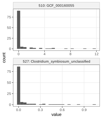
Zeller et al. (2014) sequenced stool samples to look for microbial markers of colorectal cancer. ExperimentHub record EH361 holds 1505 relative abundances (in percent, at all taxonomic levels from kingdom to strain) for 156 samples; we keep the 53 cancer and 61 tumour-free samples. Abundances are very skewed, mostly zero with a long tail (Figure 12.19).
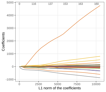
glmnet(x, y, family = "binomial") fits the lasso path of Algorithm 12.2 for 100 values of \(\lambda\) at once. At \(\lambda=0.04\) it classifies the training data almost perfectly (51 of 53 cancers, all 61 controls), but that is training error.
Questions 12.16 and 12.17
12.16. Printing the ExperimentHub object lists its thousands of records with their titles and providers; query(eh, "...") searches them.
12.17 (axes of Figure 12.20). Each curve is one coefficient \(\hat\beta_j(\lambda)\). The horizontal axis is not \(\lambda\) but the \(L_1\) norm of the fitted coefficient vector, a decreasing function of \(\lambda\); the top axis counts the non-zero coefficients. The paths are piecewise smooth, and coefficients enter (and occasionally leave) the active set at the kinks.
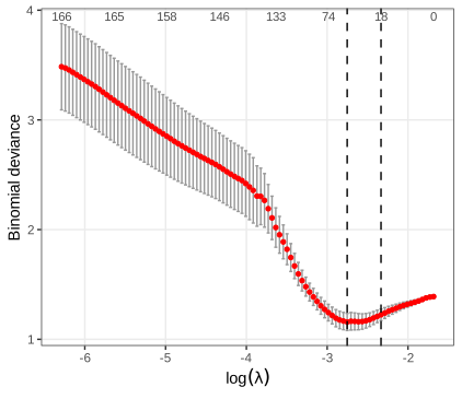
To choose \(\lambda\), cv.glmnet runs ten-fold cross-validation for every \(\lambda\) on the path (Figure 12.21).
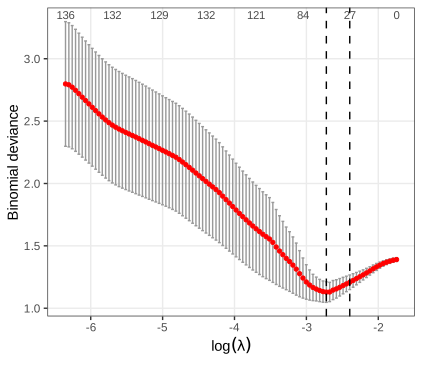
Filling the gap 12.8: what cv.glmnet computes Figures 12.21–12.23
Fix the folds \(F_1,\dots,F_K\) and the \(\lambda\) sequence of the full-data fit. For fold \(k\), fit the path to the other folds (with their own standardisation) and compute, for each held-out \(i\in F_k\), the binomial deviance \(-2[y_i\log\hat p_i+(1-y_i)\log(1-\hat p_i)]\) (twice the log loss (12.4), with \(\hat p_i\) clipped to \([10^{-5},1-10^{-5}]\)), or the misclassification indicator for type.measure = "class". Let \(\bar D_k(\lambda)\) be the mean over fold \(k\). Then
a mean and an estimated standard error over folds. \(\lambda_\text{min}\) minimises cvm; \(\lambda_\text{1se}\) is the largest \(\lambda\) with \(\mathrm{cvm}(\lambda)\)
The rule "one standard error" is a heuristic. Its rationale is the optimism of a minimum (Result 12.19): the curve is noisy, and its minimiser is biased towards too little penalisation, as the book says. Note also that \(\mathrm{cvm}(\lambda_\text{min})\) is itself an optimistic estimate of the error of the tuned procedure; an honest estimate needs an outer loop (Algorithm 12.3).
cv.glmnet.Questions 12.18–12.21
12.18. At \(\lambda_\text{1se}\) the training confusion table is the book's: 37 of 53 cancers and 55 of 61 controls correct (sensitivity 0.698, specificity 0.902, with cancer as positive).
12.19. The three largest coefficients at \(\lambda_\text{1se}\) (18 non-zero) belong to candidate division TM7 single cell isolate TM7b (\(-41.9\)), Subdoligranulum variabile (\(-6.40\)) and Lachnospiraceae bacterium 7_1_58FAA (\(-1.23\)), as in the book. The response level modelled is "n" (normal), so negative coefficients mark taxa that are more abundant in cancer samples. Their sizes are on the abundance scale: a taxon with small abundances needs a large coefficient, so the ranking reflects scale as well as importance (Exercise 12.4).
12.20. After \(\operatorname{asinh}\), which compresses the long tails, the CV curve is similar with a slightly lower minimum (deviance 1.129 against 1.158; \(\lambda_\text{min}=0.0657\), \(\lambda_\text{1se}=0.0910\)), Figure 12.22.
12.21 (screening). No. The samples are roughly half cancers; in a screening population the prevalence might be 1%. With the sensitivity and specificity above (training values, so optimistic), Result 12.11 gives \(\mathrm{PPV}\)
12.6.3 Example: classifying mouse cells from their expression profiles
Now the genotype (wild type or FGF4 knock-out) of the 53 E3.25 cells from all 45,101 probes, with misclassification as the CV measure (Figure 12.23). The error is 0.32 (the null rule, 17 knock-outs in 53) at \(\lambda_{\max}\) and falls to 0 for \(\lambda\le0.050\): the less penalisation, the better.
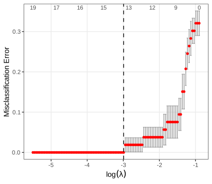
Question 12.22 (why no penalty is needed here)
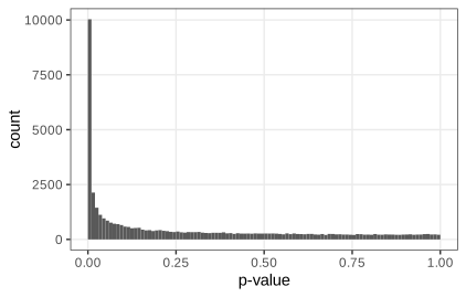
The two genotypes differ in a large fraction of the genes. The per-gene \(t\)-tests (Figure 12.24) give 22% of the p-values below 0.01, where 1% is expected under the null, and the flat right part of the histogram suggests that only about half of the genes are null: the estimate \(\hat\pi_0=\#\{p>0.5\}/(0.5\cdot m)\) (the idea of Storey 2003, Chapter 6) is 0.52. With so many informative features, an average over many of them is a stable classifier and the variance that penalisation fights is small. The one-nearest-neighbour rule on all scaled features confirms it: across all eight sample groups only 18 of the 101 cells have a nearest neighbour from another group, and the E3.25 wild type and knock-out cells are almost perfectly separated (33 of 36 and 15 of 17). Setting the self-distance to infinity, as the book does, makes this table a leave-one-out estimate (it agrees with class::knn.cv), but the scaling used all cells, and as the book notes, truly new data (another lab, another day) may behave differently.
12.7 A large choice of methods
LDA, QDA and penalised logistic regression are three of hundreds of learning algorithms in R: support vector machines (e1071::svm, kernlab::ksvm), trees and forests (rpart, randomForest), boosting (mboost), penalised discriminant analysis, and more. Two of the simplest ideas are worth a closer look, because many others refine them (Exercise 12.5).
Result 12.18 (one nearest neighbour is at most twice as bad as the best rule)
Two classes, \(\eta(\x)=\Pr(Y=1\given X=\x)\) continuous, Bayes risk \(R^*\). As \(n\to\infty\) the error of the one-nearest-neighbour rule converges to
\[ R_\text{NN}=\E\big[2\eta(X)(1-\eta(X))\big],\qquad R^*\le R_\text{NN}\le2R^*(1-R^*)\le2R^*. \]Proof (under the stated continuity)
For a test point \(\x\), its nearest training point \(\x'_n\) converges to \(\x\) almost surely as \(n\to\infty\) (for \(\x\) in the support of \(X\)), so \(\eta(\x'_n)\to\eta(\x)\). The test label \(Y\) and the neighbour's label \(Y'\) are independent given the two locations, so \(\Pr(Y\)
For \(X\) uniform on \([0,1]\) and \(\eta(x)=x\): \(R^*=\tfrac14\), \(R_\text{NN}=\tfrac13\), bound \(0.375\); a simulation with 20,000 training points gives 0.3345. The result needs \(n\) to be large compared with the dimension, which Section 12.4.2 shows is hopeless for large \(p\).
Filling the gap 12.9: support vector machines and kernels, in brief Section 12.7, Exercise 12.1
Margin. For separable data with labels \(y_i\in\{-1,1\}\), scale \((\w,b)\) so that \(\min_iy_i(\w^\T\x_i+b)=1\). The distance from \(\x_i\) to the hyperplane \(\w^\T\x+b=0\) is \(|\w^\T\x_i+b|/\|\w\|\), so the two closest classes are \(2/\|\w\|\) apart. The maximal-margin hyperplane solves \(\min\tfrac12\|\w\|^2\) subject to \(y_i(\w^\T\x_i+b)\ge1\).
Soft margin = hinge loss + ridge penalty. Allowing violations \(\xi_i\ge0\): \(\min\tfrac12\|\w\|^2+C\sum_i\xi_i\) subject to \(y_i(\w^\T\x_i+b)\ge1-\xi_i\). For fixed \((\w,b)\) the best slack is \(\xi_i=(1-y_if(\x_i))_+\), so the problem is
\[ \min_{\w,b}\ \sum_{i=1}^n\big(1-y_if(\x_i)\big)_++\frac1{2C}\|\w\|^2,\qquad f(\x)=\w^\T\x+b: \]a penalised loss exactly like Definition 12.5, with the hinge loss in place of the logistic loss.
Dual problem and kernels
The Lagrangian of the soft-margin problem with multipliers \(\alpha_i\ge0\) (margin constraints) and \(\mu_i\ge0\) (\(\xi_i\ge0\)) is \(\tfrac12\|\w\|^2\)
a convex quadratic programme. Complementary slackness gives \(\alpha_i=0\) for points strictly outside the margin: only the support vectors enter \(\w\). The data appear only through inner products, so replacing \(\x_i^\T\x_j\) by a positive semi-definite kernel \(k(\x_i,\x_j)=\bm\phi(\x_i)^\T\bm\phi(\x_j)\) fits a linear rule in the (possibly infinite-dimensional) feature space of \(\bm\phi\) at the cost of an \(n\times n\) matrix, with decision function \(f(\x)=\sum_i\alpha_iy_ik(\x_i,\x)+b\). Common kernels: linear, polynomial \((1+\x^\T\x')^d\), radial \(\exp(-\sigma\|\x-\x'\|^2\)), Laplace \(\exp(-\sigma\|\x-\x'\|)\). This is the sense of the book's footnote that kernel methods need only similarities between objects (Schölkopf, Tsuda and Vert 2004). We fit a hard-margin linear SVM with kernlab::ksvm and confirm \(\min_iy_if(\x_i)=1\) at the support vectors.
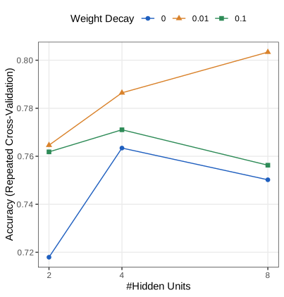
The interfaces of these packages differ, while the tasks around them (resampling, tuning, performance summaries) are the same. caret wraps 239 methods behind one interface. The book tunes a one-hidden-layer neural network (nnet) for the embryonic day from the four genes over a grid of sizes (2, 4, 8 hidden units) and weight decays (0, 0.01, 0.1), by ten-fold cross-validation repeated three times.
Filling the gap 12.10: what caret reports Figure 12.25
Repeated cross-validation. The ten-fold split is drawn three times; each configuration is fitted and evaluated on all 30 train/test splits, and the 30 accuracies are averaged. Repetition reduces the variance that comes from one particular split; it does not remove the optimism of picking the best configuration.
Accuracy and kappa. Accuracy is \(1-\widehat{\MCR}\). Cohen's kappa corrects it for agreement by chance: with \(p_o\) the observed agreement and \(p_e=\sum_k\hat\Pr(\hat Y=k)\hat\Pr(Y=k)\) the agreement expected if predictions were independent of the truth with the same marginal frequencies, \(\kappa=(p_o-p_e)/(1-p_e)\). It is 0 for a rule no better than chance (for example "always predict the largest class") and 1 for perfect prediction, which matters with unbalanced classes.
Weight decay is a ridge penalty. nnet minimises the fitting criterion plus decay times the sum of squared weights: Definition 12.5 with \(\alpha=0\), applied to a non-linear model.
Question 12.23 (will the best accuracy generalise?)
No: 0.803 is the maximum of nine noisy estimates and is biased upwards (Result 12.19). An honest estimate puts the whole tuning procedure inside an outer cross-validation loop (Algorithm 12.3; Ambroise and McLachlan 2002), and even that cannot account for choices that were never written down (Section 12.7.1).
12.7.1 Method hacking
Trying preprocessing variants, methods and tuning parameters until the result looks good is the learning analogue of p-value hacking (Chapter 6). The size of the resulting optimism has a simple bound.
Result 12.19 (the optimism of the best of \(M\) tries)
Let \(\hat A_m=A_m+\varepsilon_m\), \(m=1,\dots,M\), be accuracy estimates of \(M\) configurations, with errors \(\varepsilon_m\) that are each \(\N(0,\sigma^2)\) (or, more generally, sub-Gaussian with variance proxy \(\sigma^2\)), of any dependence. Then
\[ \E\big[\max_m\varepsilon_m\big]\le\sigma\sqrt{2\log M}. \]If all configurations are equally good (\(A_m=A\)), the reported \(\max_m\hat A_m\) overstates \(A\) by \(\E\max_m\varepsilon_m\), which can approach this bound when the estimates are nearly independent.
Proof
For any \(t>0\), by Jensen's inequality and \(e^{t\max_m\varepsilon_m}\le\sum_me^{t\varepsilon_m}\),
\[ e^{t\E\max_m\varepsilon_m}\le\E e^{t\max_m\varepsilon_m}\le\sum_m\E e^{t\varepsilon_m}=Me^{t^2\sigma^2/2}. \]Taking logarithms, \(\E\max\varepsilon_m\le\frac{\log M}t+\frac{t\sigma^2}2\); the choice \(t=\sqrt{2\log M}/\sigma\) gives the bound. ∎ For \(M=100\) independent standard normals the expected maximum is 2.51 against the bound 3.03. With 66 samples a single accuracy estimate has standard deviation around \(\sqrt{0.8\cdot0.2/66}\approx0.05\), so the best of nine configurations can be inflated by several percentage points.
Algorithm 12.3 (nested cross-validation)
- Split the data into outer folds \(O_1,\dots,O_K\).
- For each \(k\): on the data outside \(O_k\), run the entire modelling procedure, including preprocessing, feature selection and an inner cross-validation over the tuning grid, and refit the chosen configuration on all data outside \(O_k\).
- Evaluate that final model on \(O_k\). Average over \(k\).
The average estimates the error of the procedure (tuning included). It does not tell which configuration to use; for that, run the inner procedure once on all data. Choices that were made by looking at the data but are not part of the coded procedure remain outside its reach, which is why the book insists on validation with truly new data and on publishing the complete workflow (Holmes 2018).
Summary
- The target of classification is the Bayes rule; LDA and QDA estimate it with Gaussian class models (linear or quadratic boundaries, priors that shift them), logistic regression with a model of the posterior odds that LDA implies but does not need.
- Training error is optimistic, by \(2\sigma^2p/n\) for least squares, and useless when \(p\) approaches \(n\): almost every labelling is then linearly separable. Cross-validation estimates the error of a procedure trained on slightly fewer points, without bias, provided every data-driven step is inside the loop.
- Irrelevant features cost accuracy even though they do not change the Bayes error; high-dimensional space is empty, mostly boundary, and has nearly constant distances.
- Loss functions determine the optimal prediction; sensitivity, specificity and prevalence together determine predictive values; the AUC is the probability of ranking a random positive above a random negative.
- Penalisation trades bias for variance: ridge shrinks proportionally and always improves on least squares for small \(\lambda\); the lasso soft-thresholds and selects; the elastic net keeps correlated groups. The whole path is computed by coordinate descent from \(\lambda_{\max}\); \(\lambda\) is tuned by cross-validation, and the tuned error must itself be assessed by an outer loop or, better, on new data.
Exercises
The five exercises of Chapter 12 (Holmes and Huber 2019, Section 12.10), restated in my own words, with worked solutions (hidden). Numerical answers come from the course R code (results_ch12 in code/ch12_supervised_learning.R).
Exercise 12.1 (kernel SVM for the microbiome data). Apply a kernel support vector machine from
kernlabto the Zeller microbiome data. Which kernel works well?Solution
Method.
ksvm(x, disease, type = "C-svc", kernel = k, C = 1, cross = 10)with standardised features (constant features removed), for the linear, radial (\(\sigma=1/p\)), polynomial (degree 2) and Laplace (\(\sigma=1/p\)) kernels, on the raw and \(\operatorname{asinh}\) abundances, averaging the ten-fold CV error over five random fold assignments.kernel raw asinh linear 0.231 0.240 radial 0.291 0.278 polynomial, degree 2 0.434 0.435 Laplace 0.480 0.480 Interpretation. The linear kernel works best (about 23% error). With \(p=1505\gg n=114\) the data are already linearly separable (Result 12.4), so a richer feature space only adds variance; the degree-2 and Laplace kernels with default parameters are close to chance (the null rule errs on 46.5%). Kernel parameters and \(C\) should be tuned by an inner cross-validation, and the result assessed in an outer loop (Algorithm 12.3); the numbers above, without tuning, are honest but not optimal.
Exercise 12.2 (ridge versus lasso for regression). Use
glmnetto predict a continuous response: the prostate cancer data used in Chapter 3 of Hastie et al. (2008), the log PSA level (lpsa) of 97 men from eight clinical measurements. Compare ridge and lasso.Solution
Data. The package
ElemStatLearnnamed by the book has been archived; the R code reads the same data file that accompanies Hastie et al. (2008) and uses its split into 67 training and 30 test men. \(\lambda\) is chosen by ten-fold CV on the training set with the one-standard-error rule, and the test MSE is computed once.method \(\lambda\) non-zero test MSE least squares 0 8 0.521 ridge 0.900 8 0.516 lasso 0.198 5 0.473 Interpretation. Both penalties improve slightly on least squares (Result 12.15). Ridge keeps all eight predictors and shrinks them (the
lcavolcoefficient falls from 0.58 to 0.27); the lasso setsage,lcpandgleasonto zero and keepslcavol,lweight,svi,lbphand a tinypgg45, a simpler model with the lowest test error here. With only 30 test cases the differences are within noise (the test MSE has a standard error of roughly 0.1); the point is that the lasso reaches the same accuracy with fewer variables.Exercise 12.3 (smoothing as model selection). Regard the curve fitting of Figure 12.1 as regression with model selection. What plays the role of the penalty \(\lambda\) of (12.8), and how do we choose it?
Solution
For loess the tuning parameter is the span (the fraction of points in each local fit; for kernel smoothers the bandwidth). For smoothing splines it is literally a penalty: \(\hat f\)
\({}=\argmin\sum_i(y_i-f(x_i))^2+\lambda\int f''(t)^2\,\d t\). In all cases the fit is linear in \(\y\), \(\hat\y=\mathbf{H}_\lambda\y\), and \(\Tr\mathbf{H}_\lambda\) is its effective number of parameters, decreasing in the span or \(\lambda\). Choose it by cross-validation; for linear smoothers leave-one-out needs no refitting (Result 12.7), and generalised cross-validation replaces \(h_{ii}\) by \(\Tr\mathbf{H}/n\). On the 31 points of Figure 12.1, brute-force leave-one-out CV of loess falls steadily with the span: 7.61 at span 0.2, 4.79 at 0.5, 4.01 at 0.8 and 3.74 at 1. The data were generated from a quadratic, which a local-quadratic loess with a large span reproduces almost exactly, so CV correctly prefers the stiffest fit; the wiggly blue curve of Figure 12.1 is twice as bad on held-out points. (Hastie et al. 2008, Chapter 5, treat smoothing splines in this way.) Exercise 12.4 (scale invariance). In model (12.7) with \(p\ge2\), rescale one column of the data, \(\x_{\cdot\nu}\mapsto s\,\x_{\cdot\nu}\) with \(s\ne0\). What happens to \(\hat\bb\) of (12.8) without penalty (\(\lambda=0\)) and with one (\(\lambda>0\))?
Solution
Unpenalised. The linear predictor \(\beta^0+\sum_j\beta_jx_{ij}\) with the new column equals the old one under \(\tilde\beta_\nu=\beta_\nu/s\), \(\tilde\beta_j=\beta_j\) otherwise. This is a bijection of parameter spaces that preserves the likelihood, so the maximiser maps to the maximiser: \(\hat{\tilde\beta}_\nu=\hat\beta_\nu/s\), all fitted probabilities are unchanged. The model is equivariant.
Penalised. Under the same bijection the penalty \(|\tilde\beta_\nu|^q=|\beta_\nu|^q/|s|^q\) differs from \(|\beta_\nu|^q\): the new problem is the old problem with feature \(\nu\)'s penalty multiplied by \(|s|^{-q}\). For \(|s|>1\) the feature becomes cheaper and tends to enter earlier and with a larger effect, at the expense of the others; for \(|s|<1\) the reverse. The fitted probabilities change, so the rescaled fit is a different model. This is why
glmnetstandardises the columns before penalising (standardize = TRUE), which restores equivariance with respect to rescaling, and why coefficients of penalised fits must be interpreted with the feature scales in mind (Question 12.19). Numerically, all three facts hold: unpenalised \(\hat\beta_\nu\) scales by exactly \(1/s\); a lasso fit without standardisation changes (\(-0.547\) versus \(-0.317\) for \(s=10\)); with standardisation it scales exactly.Exercise 12.5 (two archetypes). It has been said that all classification methods refine one of two ideas, discriminant analysis and \(k\) nearest neighbours. In what sense is this a useful classification?
Solution
Discriminant analysis embeds objects in \(\R^p\) and partitions the space by boundaries estimated from a global model (Gaussian classes, a linear or quadratic boundary). Refinements change the space (feature expansions, kernels), the shape of the boundary (QDA, trees, neural networks) or the fitting criterion (logistic, hinge loss, penalties). Such methods have low variance and can extrapolate, at the price of model bias.
Nearest neighbours need no coordinates, only a dissimilarity, and decide locally from the training objects nearest to the new one. Kernel methods (the SVM decision function \(\sum_i\alpha_iy_ik(\x_i,\x)\)), kernel density classifiers and ensembles of trees with local leaves refine this. They have low bias but high variance and suffer most from the curse of dimensionality. Result 12.18 shows how good the simplest local rule is with unlimited data (at most twice the Bayes error), and Section 12.4.2 shows why unlimited data are never available in high dimension. The classification is useful because it locates any method on the bias-variance axis of Section 12.6: global-parametric versus local-nonparametric.
Demonstrations for this chapter
Each demonstration runs in the browser on the chapter's data (exported by the R code), with seeded random numbers where there is simulation, and links back to these notes. The ▶ Demo boxes above open them already set to the case under discussion.
| Demonstration | What you can see | Sections |
|---|---|---|
| Discriminant analysis: the Bayes rule with Gaussian classes | LDA and QDA regions on any pair of diabetes variables or all five (in the discriminant plane), the effect of the priors, the covariance ellipses, training and leave-one-out errors and the confusion table; all 44 error counts agree with MASS. Presets: 1 LDA on sspg and glucose (Fig. 12.6); 2 uniform priors (Fig. 12.7); 3 QDA; 4 all five variables (Question 12.6); 5 a weak pair. | 12.3 (Result 12.1, 12.2, 12.3), 12.3.2 |
| Learning by heart, cross-validation and the curse of dimensionality | Training versus leave-one-out error of LDA as features are added, on random labels or with informative features, on the R data sets (exact agreement) or simulated; feature selection inside versus outside the loop. Presets: 1 random labels (Fig. 12.11); 2 one data set (Fig. 12.12); 3 six informative features (Fig. 12.13); 4 more samples; 5 selection bias. | 12.4 (Result 12.4), 12.4.1 (Result 12.6, Gap 12.4), 12.4.2 (Result 12.8) |
| Ridge, lasso and elastic net: penalised logistic regression | Shrinkage functions under orthonormal design; lasso and elastic-net paths, ten-fold CV and the ROC curve for 260 microbiome species, computed in the browser and matching glmnet. Presets: 1 soft-thresholding; 2 lasso path (Fig. 12.20); 3 CV deviance (Fig. 12.21); 4 asinh (Fig. 12.22); 5 threshold and ROC. | 12.5 (Results 12.11, 12.12), 12.6.1 (Results 12.15–12.17, Algorithm 12.2), 12.6.2 |
The R code that produces every figure on this page and the demonstration data is code/ch12_supervised_learning.R (see the code index).
References
- Holmes, S. and Huber, W. (2019). Modern Statistics for Modern Biology. Cambridge University Press. Chapter 12.
- Ambroise, C. and McLachlan, G. J. (2002). Selection bias in gene extraction on the basis of microarray gene-expression data. Proceedings of the National Academy of Sciences, 99(10), 6562–6566. doi:10.1073/pnas.102102699.
- Bellman, R. E. (1961). Adaptive Control Processes: A Guided Tour. Princeton University Press.
- Clemmensen, L., Hastie, T., Witten, D. and Ersbøll, B. (2011). Sparse discriminant analysis. Technometrics, 53, 406–413.
- Friedman, J. H. (1997). On bias, variance, 0/1-loss, and the curse-of-dimensionality. Data Mining and Knowledge Discovery, 1, 55–77.
- Hastie, T., Tibshirani, R. and Friedman, J. (2008). The Elements of Statistical Learning, 2nd edition. Springer.
- Holmes, S. (2018). Statistical proof? The problem of irreproducibility. Bulletin of the American Mathematical Society, 55(1), 31–55.
- James, G., Witten, D., Hastie, T. and Tibshirani, R. (2013). An Introduction to Statistical Learning. Springer.
- Neumann, B., Walter, T., Hériché, J. K., et al. (2010). Phenotypic profiling of the human genome by time-lapse microscopy reveals cell division genes. Nature, 464(7289), 721–727.
- Ohnishi, Y., Huber, W., Tsumura, A., et al. (2014). Cell-to-cell expression variability followed by signal reinforcement progressively segregates early mouse lineages. Nature Cell Biology, 16(1), 27–37.
- Reaven, G. M. and Miller, R. G. (1979). An attempt to define the nature of chemical diabetes using a multidimensional analysis. Diabetologia, 16(1), 17–24.
- Schölkopf, B., Tsuda, K. and Vert, J.-P. (2004). Kernel Methods in Computational Biology. MIT Press.
- Storey, J. D. (2003). The positive false discovery rate: a Bayesian interpretation and the q-value. The Annals of Statistics, 31(6), 2013–2035.
- Witten, D. M. and Tibshirani, R. (2011). Penalized classification using Fisher's linear discriminant. Journal of the Royal Statistical Society: Series B, 73(5), 753–772.
- Zeller, G., Tap, J., Voigt, A. Y., et al. (2014). Potential of fecal microbiota for early-stage detection of colorectal cancer. Molecular Systems Biology, 10(11), 766. doi:10.15252/msb.20145645.
Every number quoted on this page comes from the course R code; the derivations are checked numerically.