Wavelets and Other Adaptive Methods
A function is spatially inhomogeneous when its smoothness changes with \(x\): flat stretches broken by jumps, or slow waves that turn into fast oscillations. A linear smoother with one bandwidth, or an orthogonal series cut at one frequency, must then either blur the rough parts or add wiggles to the smooth parts. Wavelets escape the dilemma because they are localised in both position and scale, so such functions are sparse in a wavelet basis: a few large coefficients carry the jumps, and all the rest are tiny. Thresholding the noisy coefficients (keep the large ones, kill the small ones) then adapts automatically, and comes within a logarithmic factor of an oracle that knows which coefficients matter. The chapter builds the Haar and Daubechies bases, proves the thresholding results, describes the Besov spaces over which these estimators are minimax, and closes with other locally adaptive rules (intersecting confidence intervals, Lepski's method) and an honest discussion of how much adaptation buys in practice.
Ch. 1 Introduction Ch. 2 The cdf and functionals Ch. 3 Bootstrap and jackknife Ch. 4 Smoothing Ch. 5 Regression Ch. 6 Density estimation Ch. 7 Normal means and minimax Ch. 8 Orthogonal functions Ch. 9 Wavelets Ch. 10 Other topics
How to read these notes
They follow the book. Sections carry the book's numbers (9.1 to 9.13), results keep the book's numbers (Theorem 9.6, Definition 9.11, ...), and every displayed equation of the book keeps its number, e.g. \((9.32)\). Equations without a number are steps the book skips.
Filling the gaps. The chapter quotes most of its results from the wavelet literature ("it can be shown", "we will not discuss the details"). For each one an orange Filling the gap box gives a complete argument, or, where the full proof is a research paper (Theorems 9.41, 9.43 and 9.50), the core calculation that explains the result, with its assumptions stated. Derivations start hidden: open one with its bar, or use the button below.
Figures and demonstrations. Every figure of the chapter that is computed is reproduced from scratch by the Python code, with Haar, Daubechies and symmlet filters built by spectral factorisation (no wavelet library). Figure 9.10, a box-and-arrow diagram of the cascade algorithm, is not; Figure 9.9, a sketch in the book, is computed here from real ICI intervals. Supplementary figures (9.S1, 9.S2, ...) illustrate the gaps and the exercises. The ▶ Demo boxes open an interactive demonstration already set to the case being discussed.
Main reference
L. Wasserman, All of Nonparametric Statistics, Springer (2006), Chapter 9, pages 197–225 (book website, with the data: www.stat.cmu.edu/~larry/all-of-nonpar). Section, equation, figure and exercise numbers below refer to this book. Further reading is listed in the references.
The explanations, derivations, figures and code are my own; equations are cited by their numbers in the book.
Companion courses
This chapter is the advanced sequel of the wavelet section of Probability and Statistical Inference (the same author's All of Statistics), and it overlaps two other courses on this site:
- Sections 9.1, 9.3, 9.4, 9.12 (the Haar basis, Haar regression, the noise estimate, the universal threshold, the discrete Haar transform): Probability and Statistical Inference, Section 21.4 (Theorem 21.13 with Filling the gap 21.13, Theorem 21.15, the oracle inequality, Theorem 21.D) and Section 21.5 (the transform is orthogonal and takes O(n) operations), with its Haar multiresolution demo.
- Section 9.4 (SURE and James–Stein): Probability and Statistical Inference, Lemma 12.C (Stein's lemma) and Theorem 12.D; Chapter 7 of this course, Normal Means and Minimax Theory (SURE, Pinsker's theorem, confidence balls), and Chapter 8, Nonparametric Inference Using Orthogonal Functions (REACT).
- Sections 9.3, 9.4, 9.8 (wavelet smoothing, the lasso): Statistical Learning: Theory and Methods, Section 5.9 (wavelet smoothing) with its wavelet shrinkage demo, and Section 3.4 (shrinkage methods, the lasso).
- Sections 9.9 and 9.10 (local bandwidths, comparison with kernel methods): Chapter 5 of this course, Section 5.4 (local regression) and Section 5.6 (variance estimation).
Where a proof there is complete, these notes state the result, sketch the argument and link to it. What this chapter adds, and where the effort goes here: smooth compactly supported wavelets (the multiresolution analysis, the two-scale relation, the Daubechies construction), the oracle inequality with its sharp constants and its limits, SureShrink, Besov spaces and why thresholding beats every linear estimator over them, confidence balls, basis pursuit, and the locally adaptive bandwidth rules of Goldenshluger–Nemirovski and Lepski.
The chapter at a glance
- 9.1 The Haar functions \(\phi,\psi_{jk}\) are an orthonormal basis of \(\Ltwo(0,1)\) (Theorem 9.6); the blocks function has few nonzero Haar coefficients (Figure 9.4), and sparsity is measured by the \(L_1\) norm (Filling the gap 9.1).
- 9.2 A multiresolution analysis gives a father wavelet and, through the two-scale relation, a mother wavelet (Theorem 9.22); Daubechies' filters come from factorising a trigonometric polynomial (Filling the gap 9.7).
- 9.3–9.4 Transform the data, estimate \(\sigma\) by the median absolute deviation, threshold. The universal threshold kills pure noise (Theorem 9.33) and is within \(2\log n+1\) of the oracle (Theorem 9.34, proved in Filling the gap 9.11); SureShrink picks a threshold per level (Filling the gap 9.12).
- 9.5–9.6 Besov norms are weighted \(\ell_p\) norms of wavelet coefficients; thresholding is minimax over Besov balls while linear estimators are not (Theorem 9.41, Filling the gap 9.14). Confidence balls exist but shrink no faster than \(n^{-1/4}\).
- 9.7–9.8 Mirroring at the boundaries; basis pursuit over a redundant dictionary (Filling the gap 9.17).
- 9.9–9.10 Intersecting confidence intervals choose a bandwidth per point with risk within a constant of the oracle (Filling the gap 9.18); adaptive methods win clearly only when the noise is low.
Notation. \(\Z\) the integers; \(f_{jk}(x)=2^{j/2}f(2^jx-k)\) (9.3); \(\langle f,g\rangle=\int fg\), \(\|f\|^2=\langle f,f\rangle\); the Fourier transform \(f^*(t)=\int e^{-ixt}f(x)\,\d x\) (9.1). \(\phi\) and \(\Phi\) are also the standard Normal density and cdf when the context says so, \(\Phib=1-\Phi\). In regression \(x_i=i/n\), \(n=2^J\), and \(\epsilon^2=\sigma^2/n\) is the noise variance of one empirical coefficient in the book's scaling.
Prerequisites. Chapter 7 (the normal means model, SURE, Pinsker's theorem) and Chapter 8 (orthogonal series estimators) of the book; the companion course's Chapter 21 is the gentle version of Sections 9.1 to 9.4.
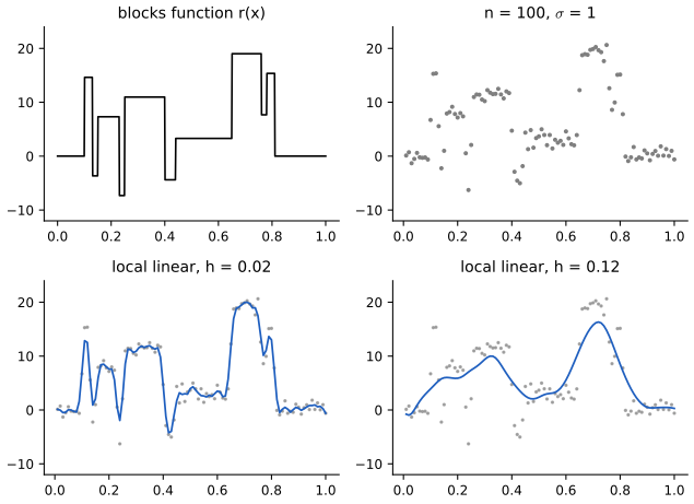
pp. 197–199 The running example is the blocks function of Donoho and Johnstone (Example 9.39): constant except for eleven jumps. With 100 noisy observations (Figure 9.1), a local linear smoother with a small bandwidth finds the jumps but is ragged between them, and one with a large bandwidth is smooth but rounds every jump away. Estimators that adjust their amount of smoothing to the location are called spatially adaptive; estimators that perform well over a large family of function classes at once are globally adaptive. The book's caveat, quoting Loader, deserves to be kept in mind: adaptation helps on problems with plenty of data and little noise, which are the easy ones (Section 9.10).
The unifying idea is sparsity: \(f=\sum_j\beta_j\phi_j\) is sparse in the basis \(\{\phi_j\}\) when most \(\beta_j\) are zero or nearly so. The \(L_2\) norm does not see sparsity: \(a=(1,0,\dots,0)\) and \(b=(n^{-1/2},\dots,n^{-1/2})\) both have \(\|a\|_2=\|b\|_2=1\), but \(\|a\|_1=1\) while \(\|b\|_1=\sqrt n\).
Filling the gap 9.1: why a small \(L_1\) norm means few important coefficients p. 199
Derivation
Let \(\theta\in\R^n\) and order the magnitudes \(|\theta|_{(1)}\ge|\theta|_{(2)}\ge\dots\). Since the \(i\) largest magnitudes are each at least \(|\theta|_{(i)}\), \(i\,|\theta|_{(i)}\le\sum_{l\le i}|\theta|_{(l)}\le\|\theta\|_1\), so \(|\theta|_{(i)}\le\|\theta\|_1/i\). Keeping the \(k\) largest coordinates (call the result \(\theta^{(k)}\)) therefore leaves
\[ \|\theta-\theta^{(k)}\|_2^2=\sum_{i>k}|\theta|_{(i)}^2\le\|\theta\|_1^2\sum_{i>k}\frac1{i^2}\le\|\theta\|_1^2\int_k^\infty\frac{\d u}{u^2}=\frac{\|\theta\|_1^2}{k}. \]So a vector of unit \(L_2\) norm with a small \(L_1\) norm is well approximated by a few of its coordinates, whatever \(n\) is. For \(b\) above the bound is \(n/k\), useless, as it should be: every coordinate of \(b\) matters equally. The same inequality with \(\ell_p\), \(p<2\), in place of \(\ell_1\) gives \(\|\theta-\theta^{(k)}\|_2^2\le C_p\|\theta\|_p^2k^{1-2/p}\), which is the mechanism behind the Besov results of Section 9.5. ∎
The Fourier transform and the dilation notation are fixed once for the chapter:
\[ f^*(t)=\int_{-\infty}^{\infty}e^{-ixt}f(x)\,\d x, \tag{9.1} \] \[ f(x)=\frac1{2\pi}\int_{-\infty}^{\infty}e^{ixt}f^*(t)\,\d t\quad\text{(when \(f^*\) is integrable)}, \tag{9.2} \] \[ f_{jk}(x)=2^{j/2}f(2^jx-k). \tag{9.3} \]The factor \(2^{j/2}\) makes \(\|f_{jk}\|=\|f\|\): substitute \(u=2^jx-k\) in \(\int2^jf(2^jx-k)^2\,\d x\).
9.1 Haar Wavelets
pp. 199–202 The Haar father wavelet (scaling function) and mother wavelet are
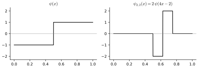
\[ \phi(x)=\begin{cases}1&0\le x<1\\0&\text{otherwise,}\end{cases} \tag{9.4} \] \[ \psi(x)=\begin{cases}-1&0\le x\le\tfrac12\\ 1&\tfrac12<x\le1.\end{cases} \tag{9.5} \]\(\psi_{jk}\) is \(\psi\) squeezed onto \([k2^{-j},(k+1)2^{-j}]\) and raised to height \(2^{j/2}\) (Figure 9.2). Let \(W_j=\{\psi_{jk}:k=0,\dots,2^j-1\}\), the level-\(j\) wavelets on \([0,1]\).
Theorem 9.6 (the Haar basis) p. 200
\(\{\phi,W_0,W_1,W_2,\dots\}\) is an orthonormal basis of \(\Ltwo(0,1)\). Hence every \(f\in\Ltwo(0,1)\) satisfies
\[ f(x)=\alpha\,\phi(x)+\sum_{j=0}^\infty\sum_{k=0}^{2^j-1}\beta_{jk}\psi_{jk}(x),\qquad \alpha=\int_0^1f\phi,\quad\beta_{jk}=\int_0^1f\psi_{jk}, \tag{9.7} \]with convergence in \(\Ltwo\). The scaling coefficient is \(\alpha\), the \(\beta_{jk}\) are the detail coefficients, and the resolution-\(J\) approximation
\[ f_J(x)=\alpha\,\phi(x)+\sum_{j=0}^{J-1}\sum_{k=0}^{2^j-1}\beta_{jk}\psi_{jk}(x) \tag{9.8} \]has \(1+\sum_{j<J}2^j=2^J\) terms.
Filling the gap 9.2: proof of Theorem 9.6 (Exercise 2), sketched; full proof in the companion course p. 200
Proof
Orthonormality. \(\|\psi_{jk}\|=\|\psi\|=1\) by the remark after (9.3). Two wavelets at the same level have disjoint supports. If \(j<j'\), the support of \(\psi_{j'k'}\) is a dyadic interval of length \(2^{-j'}\) that lies inside one half of the support of \(\psi_{jk}\) or outside it, so \(\psi_{jk}\) is constant there and \(\langle\psi_{jk},\psi_{j'k'}\rangle=c\int\psi_{j'k'}=0\). Likewise \(\langle\phi,\psi_{jk}\rangle=\int\psi_{jk}=0\).
Completeness. Let \(V_J\) be the functions on \([0,1)\) that are constant on each \([k2^{-J},(k+1)2^{-J})\), a space of dimension \(2^J\). The \(2^J\) orthonormal functions \(\phi,\psi_{jk}\) (\(j<J\)) all lie in \(V_J\), so they are a basis of it, and \(f_J\) is the orthogonal projection of \(f\) on \(V_J\): the function equal to the average of \(f\) on each dyadic interval of length \(2^{-J}\). Dyadic step functions are dense in \(\Ltwo(0,1)\) (continuous functions are dense, and a continuous function on \([0,1]\) is uniformly continuous, so its dyadic averages converge to it uniformly). Hence \(\|f-f_J\|\to0\), and an orthonormal system whose span is dense is a basis. All steps in full: Probability and Statistical Inference, Filling the gap 21.13; checked numerically in the course code. ∎
See also (companion course): Probability and Statistical Inference, Theorem 21.13 and its Haar multiresolution demo.
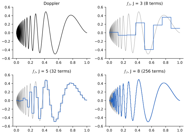
Example 9.9. For the Doppler function, \(f_J\) with \(J=3,5,8\) (Figure 9.3) is the dyadic average of \(f\) at resolution \(2^{-J}\): even 256 terms leave the fastest oscillations near 0 unresolved, because the Haar approximation spends the same resolution everywhere.
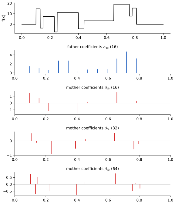
Because \(\psi_{jk}\) is localised, a blip can be added in one place without wiggles elsewhere. The Haar coefficients of blocks (Figure 9.4) are zero except for the wavelets whose support contains a jump: at most one per jump and level.
9.2 Constructing Wavelets
pp. 203–206 Haar wavelets are localised but discontinuous. Smooth, localised wavelets come from a multiresolution analysis. Given \(\phi\), let
\[ V_0=\Big\{f=\sum_{k\in\Z}c_k\phi(x-k):\ \sum_kc_k^2<\infty\Big\},\quad V_1=\{g(2x):g\in V_0\},\quad V_2=\{g(2x):g\in V_1\},\ \dots \tag{9.10} \]Definition 9.11 (multiresolution analysis) p. 203
\(\phi\) generates a multiresolution analysis (MRA) of \(\R\) if
\[ V_j\subset V_{j+1},\ j\ge0, \tag{9.12} \] \[ \textstyle\bigcup_{j\ge0}V_j\ \text{is dense in}\ \Ltwo(\R). \tag{9.13} \]\(\phi\) is then the father wavelet. As used in Lemma 9.14, one also requires (the book leaves it implicit; see Notes on the book) that the translates \(\{\phi(x-k)\}_{k\in\Z}\) are orthonormal.
Lemma 9.14 and Example 9.15 p. 203
If \(\{\phi(\cdot-k)\}\) is orthonormal, \(\{\phi_{jk}:k\in\Z\}\) is an orthonormal basis of \(V_j\). For the Haar \(\phi\), \(V_j\) is the set of \(\Ltwo\) functions constant on every \([k2^{-j},(k+1)2^{-j})\), and these spaces form an MRA.
Filling the gap 9.3: Lemma 9.14, and the Haar MRA (Exercise 3) p. 203
Proof
Lemma 9.14. The dilation \(D_jg(x)=2^{j/2}g(2^jx)\) is a linear bijection of \(\Ltwo(\R)\) that preserves inner products (substitute \(u=2^jx\)). By (9.10), \(V_j=\{g(2^jx):g\in V_0\}=D_jV_0\), and \(D_j\) maps \(\phi(\cdot-k)\) to \(\phi_{jk}\). An isometry maps an orthonormal basis of \(V_0\) to an orthonormal basis of its image, so \(\{\phi_{jk}\}_k\) is an orthonormal basis of \(V_j\). (\(V_0\) is closed: by orthonormality of the translates, \(c\mapsto\sum c_k\phi(\cdot-k)\) is an isometry from \(\ell_2\), whose image is complete.)
Haar. The translates \(\phi(x-k)=I(k\le x<k+1)\) have disjoint supports and unit norm, so they are orthonormal, and \(V_0\) is the set of square-integrable functions constant on each \([k,k+1)\); by dilation \(V_j\) is as stated. Nesting: a function constant on each interval of length \(2^{-j}\) is constant on each half of it, so \(V_j\subset V_{j+1}\). Density: continuous functions with compact support are dense in \(\Ltwo(\R)\); such a \(g\) is uniformly continuous, so its averages over the dyadic intervals of length \(2^{-j}\) (an element of \(V_j\)) converge to \(g\) uniformly on a fixed compact set containing all the supports, hence in \(\Ltwo\). ∎
Since \(\phi\in V_0\subset V_1\) and \(\{\phi_{1k}\}\) is a basis of \(V_1\),
\[ \phi(x)=\sum_k\ell_k\,\phi_{1k}(x)=\sqrt2\sum_k\ell_k\,\phi(2x-k),\qquad\ell_k=\int\phi\,\phi_{1k},\quad\sum_k\ell_k^2<\infty, \tag{9.16} \]the two-scale relation (dilation equation); for Haar \(\ell_0=\ell_1=2^{-1/2}\) and all other \(\ell_k=0\) (Exercise 1). In Fourier terms,
\[ \phi^*(t)=m_0(t/2)\,\phi^*(t/2),\qquad m_0(t)=\frac1{\sqrt2}\sum_k\ell_ke^{-itk}. \tag{9.17} \]Filling the gap 9.4: equation (9.17) (Exercise 4) and the infinite product p. 204
Derivation
Take Fourier transforms term by term in (9.16) (legitimate in \(\Ltwo\), and pointwise if \(\phi\in L_1\) and only finitely many \(\ell_k\neq0\)). With \(u=2x-k\),
\[ \int e^{-ixt}\sqrt2\,\phi(2x-k)\,\d x=\frac{\sqrt2}{2}\int e^{-i(u+k)t/2}\phi(u)\,\d u=\frac{1}{\sqrt2}e^{-ikt/2}\phi^*(t/2). \]Summing with weights \(\ell_k\): \[\phi^*(t)=\big(\tfrac1{\sqrt2}\sum_k\ell_ke^{-ik(t/2)}\big)\phi^*(t/2)=m_0(t/2)\phi^*(t/2)\]. Applying this \(m\) times,
\[ \phi^*(t)=\Big(\prod_{k=1}^m m_0(t/2^k)\Big)\,\phi^*(t/2^m)\ \xrightarrow[m\to\infty]{}\ \Big(\prod_{k=1}^\infty m_0(t/2^k)\Big)\phi^*(0), \]using continuity of \(\phi^*\) at 0 (true for \(\phi\in L_1\)). There is one factor \(m_0(t/2^k)\) per \(k\ge1\); the book's display repeats \(m_0(t/2)\) in front of the product (Notes on the book). If \(\int\phi=\phi^*(0)=1\) this is (9.20). Numerically, for the Daubechies \(N=2\) filter the truncated product at \(t=3\) agrees with the transform of the cascade-computed \(\phi\) to \(2\times10^{-3}\), the resolution of the grid. ∎
Theorem 9.18 (a father wavelet from its scaling coefficients) p. 204
Given \(\{\ell_k\}\) with \(m_0\) as in (9.19), let \(\phi^*(t)=\prod_{j\ge1}m_0(t/2^j)\) (9.20) and let \(\phi\) be its inverse Fourier transform. Suppose \(\tfrac1{\sqrt2}\sum_{k=N_0}^{N_1}\ell_k=1\) (9.21) with \(\ell_k=0\) outside \([N_0,N_1]\), that \(|m_0(t)|^2+|m_0(t+\pi)|^2=1\), that \(m_0(t)\neq0\) for \(|t|\le\pi/2\), and that \(|\phi(x)|\le\Phi(|x|)\) for a bounded, nonincreasing, integrable \(\Phi\). Then \(\phi\) is a compactly supported father wavelet, zero outside \([N_0,N_1]\).
Filling the gap 9.5: where the conditions of Theorem 9.18 come from p. 204
Derivation
(9.21) is \(m_0(0)=1\). The infinite product can converge to a nonzero limit at small \(t\) only if its factors tend to 1, i.e. \(m_0(0)=\tfrac1{\sqrt2}\sum\ell_k=1\). Then \(\phi^*(0)=1\), i.e. \(\int\phi=1\). Since \(m_0\) is a trigonometric polynomial, \(|m_0(s)-1|\le C|s|\), so \(\sum_k|m_0(t/2^k)-1|\le C|t|\) and the product converges uniformly on compacts.
The quadrature-mirror condition is necessary for orthonormal translates. By Plancherel, \[\langle\phi,\phi(\cdot-k)\rangle=\frac1{2\pi}\int|\phi^*(t)|^2e^{ikt}\d t=\frac1{2\pi}\int_0^{2\pi}A(t)e^{ikt}\d t\] with \(A(t)=\sum_{m\in\Z}|\phi^*(t+2\pi m)|^2\). The translates are orthonormal iff all these Fourier coefficients of the \(2\pi\)-periodic \(A\) equal \(\delta_{k0}\), i.e. iff \(A\equiv1\). Insert (9.17), split \(m\) into even and odd, and use that \(m_0\) has period \(2\pi\):
\[ A(2t)=\sum_m|m_0(t+\pi m)|^2|\phi^*(t+\pi m)|^2=|m_0(t)|^2A(t)+|m_0(t+\pi)|^2A(t+\pi). \]With \(A\equiv1\) this is \(|m_0(t)|^2+|m_0(t+\pi)|^2=1\). In terms of the coefficients it says \(\sum_k\ell_k\ell_{k+2m}=\delta_{m0}\): the even translates of the filter are orthonormal (checked numerically for all the filters used here). The remaining conditions (no zero of \(m_0\) on \([-\pi/2,\pi/2]\), the decay bound) are Cohen's sufficient conditions that rule out degenerate solutions such as \(\ell_0=\ell_3=2^{-1/2}\), which satisfies the identity but gives \(\phi=\tfrac13I_{[0,3)}\), whose translates are not orthonormal.
Support. \(\phi\) is the limit of the cascade iteration \(\phi^{(m+1)}(x)=\sqrt2\sum_k\ell_k\phi^{(m)}(2x-k)\) started from the Haar \(\phi^{(0)}\) (this is what (9.20) computes, since each step multiplies the transform by \(m_0(t/2)\)). If \(\phi^{(m)}\) vanishes outside \([a_m,b_m]\), then \(\phi^{(m+1)}\) vanishes outside \([(a_m+N_0)/2,(b_m+N_1)/2]\). The endpoints obey \(b_{m+1}=(b_m+N_1)/2\to N_1\) and \(a_{m+1}\to N_0\), so the limit vanishes outside \([N_0,N_1]\). ∎
Let \(W_j\) be the orthogonal complement of \(V_j\) in \(V_{j+1}\): \(V_{j+1}=V_j\oplus W_j\), hence \[\Ltwo(\R)=\overline{\bigcup_jV_j}=V_0\oplus W_0\oplus W_1\oplus\cdots\]. The mother wavelet is
\[ \psi(x)=\sqrt2\sum_k(-1)^{k+1}\ell_{1-k}\,\phi(2x-k). \]Theorem 9.22 (the wavelet basis) p. 205
\(\{\psi_{jk}:k\in\Z\}\) is an orthonormal basis of \(W_j\), and \(\{\phi_{0k},\psi_{jk}:k\in\Z,\ j\in\Z_+\}\) (9.23) is an orthonormal basis of \(\Ltwo(\R)\):
\[ f=\sum_k\alpha_{0k}\phi_{0k}+\sum_{j\ge0}\sum_k\beta_{jk}\psi_{jk},\qquad\alpha_{0k}=\int f\phi_{0k},\ \beta_{jk}=\int f\psi_{jk}. \tag{9.24} \]Starting at a level \(j_0\) instead of 0 changes nothing.
Filling the gap 9.6: proof of Theorem 9.22 p. 205
Proof
By dilation (as in Filling the gap 9.3) it suffices to treat \(j=0\): show that \(\{\psi(\cdot-k)\}\) is an orthonormal basis of \(W_0\). Every \(f\in V_1\) is \(f(x)=\sqrt2\sum_kc_k\phi(2x-k)\) with \(c\in\ell_2\), so \(f^*(t)=c^\sharp(t/2)\phi^*(t/2)\) where \(c^\sharp(s)=\tfrac1{\sqrt2}\sum c_ke^{-iks}\). Write \(m_1(s)\) for the symbol of \(\psi\): from its definition, \(m_1(s)=e^{-is}\,\overline{m_0(s+\pi)}\) (substitute \(k\to1-k\) and use \(e^{-i\pi k}=(-1)^k\)).
The modulation matrix is unitary. For \(s\in\R\) let \[M(s)=\begin{pmatrix}m_0(s)&m_0(s+\pi)\\m_1(s)&m_1(s+\pi)\end{pmatrix}\]. Its rows have unit length by the quadrature-mirror identity (the second row because \(|m_1(s)|=|m_0(s+\pi)|\)), and they are orthogonal: \[m_0(s)\overline{m_1(s)}+m_0(s+\pi)\overline{m_1(s+\pi)}=e^{is}m_0(s)m_0(s+\pi)-e^{is}m_0(s+\pi)m_0(s)=0\].
Inner products by periodisation. For \(f,g\in V_1\) with symbols \(c^\sharp,d^\sharp\), Plancherel, the substitution \(t=2s\) and the identity \(A\equiv1\) of Filling the gap 9.5 give
\[ \langle f(\cdot-k),g\rangle=\frac1\pi\int_0^{2\pi}e^{-2iks}c^\sharp(s)\overline{d^\sharp(s)}\,\d s=\frac1\pi\int_0^{\pi}e^{-2iks}B(s)\,\d s,\qquad B(s)=c^\sharp\overline{d^\sharp}(s)+c^\sharp\overline{d^\sharp}(s+\pi). \]These are the Fourier coefficients of the \(\pi\)-periodic function \(B\). So the translates of \(f\) are orthonormal iff \(|c^\sharp(s)|^2+|c^\sharp(s+\pi)|^2=1\) (take \(g=f\)), and every translate of \(f\) is orthogonal to \(g\) and its translates iff \(B\equiv0\). With \(c^\sharp=m_1\), \(d^\sharp=m_0\) these are exactly the unitarity relations: the \(\psi(\cdot-k)\) are orthonormal and orthogonal to \(V_0\), so they lie in \(W_0\).
They span \(W_0\). Given \(f\in V_1\) with symbol \(c^\sharp\), solve
\[ \big(c^\sharp(s),c^\sharp(s+\pi)\big)=a(2s)\big(m_0(s),m_0(s+\pi)\big)+b(2s)\big(m_1(s),m_1(s+\pi)\big) \]for \(\pi\)-periodic \(a,b\) (functions of \(2s\)): unitarity of \(M\) gives \(a,b\) explicitly, square-integrable over a period. This writes \(f=\sum a_k\phi(\cdot-k)+\sum b_k\psi(\cdot-k)\), i.e. \(V_1=V_0\oplus\overline{\mathrm{span}}\{\psi(\cdot-k)\}\). Hence the span of the \(\psi(\cdot-k)\) is \(W_0\). Finally \(V_J=V_0\oplus W_0\oplus\dots\oplus W_{J-1}\), and density (9.13) turns the union into \(\Ltwo(\R)\), proving (9.24). ∎
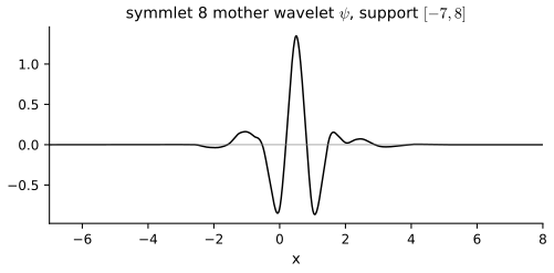
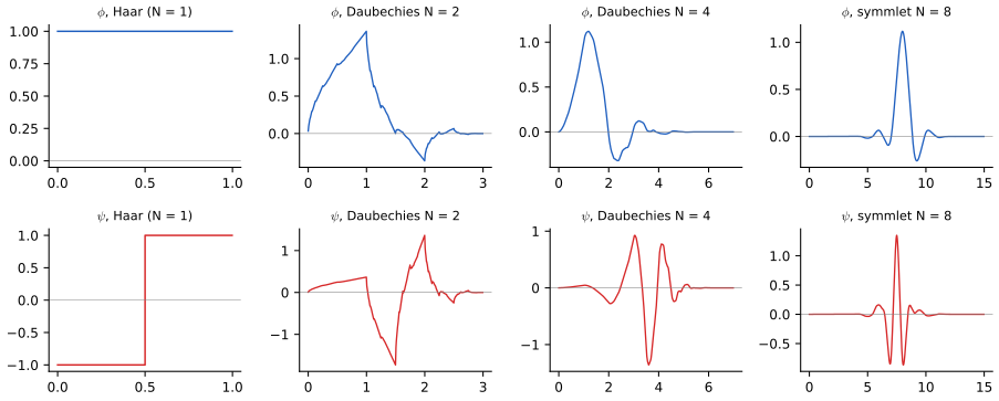
Clever choices of \(\{\ell_k\}\) give useful wavelets. Daubechies' symmlets are smooth, compactly supported and nearly symmetric (no smooth compactly supported orthonormal wavelet is exactly symmetric); the father symmlet of order \(N\) lives on \([0,2N-1]\), the mother on \([-N+1,N]\), the mother has \(N\) vanishing moments \(\int x^p\psi=0\), \(p=0,\dots,N-1\), and smoothness grows with \(N\). The book lists the 16 coefficients of the symmlet 8; the course code constructs them from scratch and recovers the printed values to \(5\times10^{-11}\).
Filling the gap 9.7: the Daubechies construction, vanishing moments and symmlets pp. 205–206
Derivation
Vanishing moments are zeros of \(m_0\) at \(\pi\). \(\psi^*(t)=m_1(t/2)\phi^*(t/2)\) and \(\int x^p\psi(x)\,\d x=i^p(\psi^*)^{(p)}(0)\). Since \(\phi^*(0)=1\), \(\psi^*\) has a zero of order \(N\) at 0 iff \(m_1\) does, iff \(m_0\) has a zero of order \(N\) at \(\pi\) (because \(|m_1(s)|=|m_0(s+\pi)|\)). So write \(m_0(t)=\big(\tfrac{1+e^{-it}}2\big)^NL(t)\) with \(L\) a trigonometric polynomial, \(L(0)=1\).
Reducing to a polynomial identity. With \(y=\sin^2(t/2)\), \(|\tfrac{1+e^{-it}}2|^2=\cos^2(t/2)=1-y\), and \(|L(t)|^2\), being even and real, is a polynomial \(P(y)\). Replacing \(t\) by \(t+\pi\) swaps \(y\) and \(1-y\), so the quadrature-mirror identity becomes
\[ (1-y)^NP(y)+y^NP(1-y)=1,\qquad y\in[0,1]. \]The minimal solution. Expand \[1=\big((1-y)+y\big)^{2N-1}=\sum_{k=0}^{2N-1}\binom{2N-1}{k}y^k(1-y)^{2N-1-k}\]. The terms with \(k\le N-1\) contain \((1-y)^N\), the others contain \(y^N\), and the map \(k\mapsto2N-1-k\) exchanges the two groups while swapping \(y\) and \(1-y\). Hence \(P(y)=\sum_{k=0}^{N-1}\binom{2N-1}{k}y^k(1-y)^{N-1-k}\) solves the identity; it equals \(\sum_{k=0}^{N-1}\binom{N-1+k}{k}y^k\) (both are the unique solution of degree below \(N\), by Bézout's theorem, since \((1-y)^N\) and \(y^N\) are coprime). \(P\ge0\) on \([0,1]\).
Spectral factorisation. It remains to find \(L\) with \(|L(t)|^2=P(\sin^2(t/2))\). Each root \(y_r\) of \(P\) gives, through \(\sin^2(t/2)=(2-z-z^{-1})/4\) with \(z=e^{it}\), a pair of roots \(z_r,1/z_r\) of \(z+z^{-1}=2-4y_r\). Choosing one root from each pair (both members of a complex-conjugate pair together, so that the \(\ell_k\) are real) and setting \(L(t)\propto\prod_r(e^{-it}-z_r)\) gives \(|L|^2\propto P\). Taking all roots inside the unit circle is Daubechies' extremal-phase choice; trying all admissible choices and keeping the one whose phase is closest to linear gives the least asymmetric wavelet, the symmlet. For \(N=8\) there are \(2^4=16\) choices; the one with the most nearly linear phase reproduces the book's coefficients (the code in daubechies_filter). The resulting filter has \(2N\) coefficients, so by Filling the gap 9.5 the father wavelet lives on \([0,2N-1]\), and the mother on an interval of the same length, \([-N+1,N]\) after the shift used in the book. ∎
9.3 Wavelet Regression
pp. 206–208 The model is
\[ Y_i=r(x_i)+\sigma\epsilon_i,\qquad\epsilon_i\sim N(0,1),\quad x_i=i/n,\quad n=2^J. \tag{9.25} \]Approximate \(r\) by \(n\) terms,
\[ r(x)\approx r_n(x)=\sum_{k=0}^{2^{j_0}-1}\alpha_{j_0,k}\phi_{j_0,k}(x)+\sum_{j=j_0}^{J}\sum_{k=0}^{2^j-1}\beta_{jk}\psi_{jk}(x), \tag{9.26} \]and estimate the coefficients by the empirical scaling and detail coefficients
\[ S_k=\frac1n\sum_i\phi_{j_0,k}(x_i)Y_i,\qquad D_{jk}=\frac1n\sum_i\psi_{jk}(x_i)Y_i, \tag{9.27} \]which are approximately \(N(\alpha_{j_0,k},\sigma^2/n)\) and \(N(\beta_{jk},\sigma^2/n)\). In practice (the book's footnote 2) one sets the finest scaling coefficients to \(Y_k/\sqrt n\) and runs the cascade algorithm of Section 9.12; equivalently, one applies the orthonormal discrete wavelet transform to the vector \(\bY\), obtaining coefficients that are \(\sqrt n\) times the above, with noise standard deviation exactly \(\sigma\). The code and the demos use this second scaling. The noise level is estimated robustly from the finest level,
\[ \hs=\sqrt n\times\frac{\median\{|D_{J-1,k}-\median_k D_{J-1,k}|:k=0,\dots,2^{J-1}-1\}}{0.6745}, \]the scaling coefficients are not shrunk, \(\hat\alpha_{j_0,k}=S_k\), and the detail coefficients are thresholded (Section 9.4).
Filling the gap 9.8: why \(Y_k/\sqrt n\) approximates \(\alpha_{J,k}\), and why the noise stays white p. 207, footnote 2
Derivation
The approximation. Let \(\phi\) have support \([0,L]\) and \(\int\phi=1\), and let \(r\) be Lipschitz with constant \(M\). Substituting \(u=nx-k\) in \(\alpha_{J,k}=\int r\,\phi_{J,k}\) with \(2^J=n\),
\[ \sqrt n\,\alpha_{J,k}-r(k/n)=\int_0^L\big[r((u+k)/n)-r(k/n)\big]\phi(u)\,\d u,\qquad\big|\sqrt n\,\alpha_{J,k}-r(k/n)\big|\le\frac{M}{n}\int_0^Lu|\phi(u)|\,\d u. \]So each finest-level coefficient is off by \(O(n^{-3/2})\) in the book's scaling, and the total squared error of the \(n\) of them, which the orthonormal cascade carries unchanged to all other coefficients, is \(O(n\cdot n^{-3})=O(n^{-2})\): negligible against the statistical error. For Haar, \(L=1\) and the bound is \(M/(2n)\); at a jump the error is of the size of the jump but affects only the few coefficients near it.
The noise. The discrete transform is an orthogonal \(n\times n\) matrix \(W\) (Filling the gap 9.22). If \(\epsilon\sim N(0,\sigma^2I)\), then \(W\epsilon\sim N(0,\sigma^2WW^\T)=N(0,\sigma^2I)\): the noise in the empirical coefficients is exactly independent and \(N(0,\sigma^2)\), not merely approximately. Details for Haar: Probability and Statistical Inference, Filling the gap 21.14. ∎
Filling the gap 9.9: the median absolute deviation estimate of \(\sigma\) p. 207
Derivation
If \(Z\sim N(0,\sigma^2)\), the median of \(|Z|\) is \(\sigma\Phi^{-1}(3/4)=0.6745\,\sigma\). At the finest level most \(\beta_{J-1,k}\) are negligible (they decay like \(2^{-J(s+1/2)}\) for a function of smoothness \(s\), Filling the gap 9.13), so the \(m=n/2\) coefficients are mostly pure noise. The sample median of \(|D-\median D|\) is consistent for the population median under such a mixture as long as the fraction of large coefficients tends to 0: a median moves by at most the fraction of contaminated observations divided by the density at the median. A few large coefficients at jumps (a fixed number \(K\)) shift it by \(O(K/n)\), while a standard deviation computed from the same coefficients could be ruined by a single one. On pure noise with \(n=2^{14}\) the estimate is within 3 percent of \(\sigma\) (course code). More: Probability and Statistical Inference, Filling the gap 21.15. ∎
9.4 Wavelet Thresholding
pp. 208–211 Writing
\[ D_{jk}\approx\beta_{jk}+\frac{\sigma}{\sqrt n}\epsilon_{jk}, \tag{9.28} \]the linear shrinkers of Chapters 7 and 8, \(\hb_{jk}=cD_{jk}\), are replaced by thresholding: the hard and soft thresholds
\[ \hb_{jk}=\begin{cases}0&|D_{jk}|<\lambda\\D_{jk}&|D_{jk}|\ge\lambda,\end{cases} \tag{9.29} \] \[ \hb_{jk}=\begin{cases}D_{jk}+\lambda&D_{jk}<-\lambda\\0&-\lambda\le D_{jk}<\lambda\\D_{jk}-\lambda&D_{jk}>\lambda,\end{cases} \tag{9.30} \] \[ \hb_{jk}=\sgn(D_{jk})\,(|D_{jk}|-\lambda)_+. \tag{9.31} \]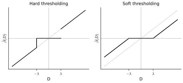
The simplest threshold is the universal threshold
\[ \lambda=\sigma\sqrt{\frac{2\log n}{n}}. \tag{9.32} \]Theorem 9.33 (pure noise is removed) p. 209
If all \(\beta_{jk}=0\), the soft-threshold estimator with the universal threshold satisfies \(\P(\hb_{jk}=0\text{ for all }j,k)\to1\).
Filling the gap 9.10: the proof of Theorem 9.33 with its rate p. 210
Proof
With \(\sigma\) known and the exact transform, the \(n-1\) detail coefficients are independent \(N(0,\sigma^2/n)\) (Filling the gap 9.8), and \(\hb_{jk}=0\) iff \(|D_{jk}|\le\lambda\). Mills' inequality, \(\P(|Z|>t)\le\sqrt{2/\pi}\,e^{-t^2/2}/t\), with \(t=\sqrt n\lambda/\sigma=\sqrt{2\log n}\) (so \(e^{-t^2/2}=1/n\)) and a union bound give
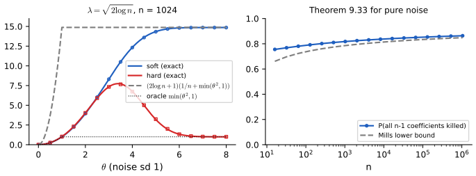
\[ \P\big(\max_{j,k}|D_{jk}|>\lambda\big)\le(n-1)\sqrt{\frac2\pi}\,\frac{1/n}{\sqrt{2\log n}}\le\frac{\sqrt{2/\pi}}{\sqrt{2\log n}}\to0. \](The book's chain writes "=" where Mills' inequality gives "\(\le\)", and the factor \(n\) from the sum cancels the \(1/n\).) The convergence is very slow. By independence the probability is exactly \((1-2\Phib(\sqrt{2\log n}))^{n-1}\): 0.82 for \(n=1024\) and 0.86 for \(n=2^{20}\) (Figure 9.S2, right). With \(\hs\) in place of \(\sigma\), one needs \(\hs/\sigma=1+\OP(n^{-1/2})\) to keep \(\sqrt{2\log n}\,(\hs/\sigma-1)\to0\); see Probability and Statistical Inference, Filling the gap 21.16. ∎
Theorem 9.34 (Donoho and Johnstone 1994: the oracle inequality) p. 210
Let \(X_i=\theta_i+\frac{\sigma}{\sqrt n}\epsilon_i\), \(i=1,\dots,n\). For \(S\subset\{1,\dots,n\}\) the "kill it or keep it" estimator is \(\hat\theta_S=(X_1I(1\in S),\dots,X_nI(n\in S))\), and the oracle risk is
\[ R_n^*=\min_SR(\hat\theta_S,\theta) \tag{9.35} \] \[ \phantom{R_n^*}=\sum_{i=1}^n\Big(\theta_i^2\wedge\frac{\sigma^2}{n}\Big). \tag{9.36} \]If \(\hat\theta=(t(X_1),\dots,t(X_n))\) with \(t(x)=\sgn(x)(|x|-\lambda_n)_+\) and \(\lambda_n=\sigma\sqrt{2\log n/n}\), then for every \(\theta\in\R^n\)
\[ R(\hat\theta,\theta)\le(2\log n+1)\Big(\frac{\sigma^2}{n}+R_n^*\Big). \tag{9.37} \]The book also prints \(R_n^*\le R(\hat\theta,\theta)\) on the left of (9.37); that half is false (Notes on the book).
Filling the gap 9.11: the oracle risk (9.36) and the oracle inequality (9.37) p. 210
Proof
Write \(\epsilon^2=\sigma^2/n\) for the noise variance. (9.36). The risk of \(\hat\theta_S\) is a sum over coordinates: keeping \(i\) costs \(\E(X_i-\theta_i)^2=\epsilon^2\), killing it costs \(\theta_i^2\). The coordinates can be chosen separately, so the best \(S\) keeps exactly the \(i\) with \(\theta_i^2>\epsilon^2\) and \(R_n^*=\sum_i\min(\theta_i^2,\epsilon^2)\). (This is Exercise 7(a).)
One coordinate, unit noise. Let \(X\sim N(\theta,1)\) and \(r(\theta)=\E(t(X)-\theta)^2\) with threshold \(\lambda\). Three facts.
(a) \(r'(\theta)=2\theta\,\P_\theta(|X|\le\lambda)\). Differentiate under the expectation (\(t\) is Lipschitz with \(t'(x)=I(|x|>\lambda)\)): \[r'(\theta)=2\E[(t(X)-\theta)(t'(X)-1)]=-2\E[(t(X)-\theta)I(|X|\le\lambda)]=2\theta\P(|X|\le\lambda)\], because \(t(X)=0\) on that event. So \(r\) is even, increasing in \(|\theta|\), and tends to \(1+\lambda^2\) (for large \(\theta\), \(t(X)=X-\lambda\) with probability near one): \(r(\theta)\le1+\lambda^2\).
(b) \(r(\theta)\le r(0)+\theta^2\): for \(\theta\ge0\), \[r(\theta)-r(0)=\int_0^\theta2u\,\P_u(|X|\le\lambda)\,\d u\le\theta^2\].
(c) \(r(0)\le4\phi(\lambda)/\lambda^3\). At \(\theta=0\), \[r(0)=2\int_\lambda^\infty(z-\lambda)^2\phi(z)\,\d z=2\int_0^\infty w^2\phi(\lambda+w)\,\d w\], and \(\phi(\lambda+w)\le\phi(\lambda)e^{-\lambda w}\), so \[r(0)\le2\phi(\lambda)\int_0^\infty w^2e^{-\lambda w}\d w=4\phi(\lambda)/\lambda^3\].
Assembling. With \(\lambda=\sqrt{2\log n}\), \(\phi(\lambda)=1/(n\sqrt{2\pi})\) and, for \(n\ge2\), \(\lambda^3\ge1.6\), so \(r(0)\le4/(1.6\sqrt{2\pi}\,n)\le1/n\). By (a) and (b), \[r(\theta)\le\min(r(0)+\theta^2,1+\lambda^2)\le r(0)+\min(\theta^2,1+\lambda^2)\le(1+\lambda^2)\big(\tfrac1n+\min(\theta^2,1)\big)\]. For noise level \(\epsilon\), scale: the risk in coordinate \(i\) is \[\epsilon^2r(\theta_i/\epsilon)\le(1+\lambda^2)\big(\epsilon^2/n+\min(\theta_i^2,\epsilon^2)\big)\]. Summing over \(i\): \[R(\hat\theta,\theta)\le(2\log n+1)(\epsilon^2+R_n^*)=(2\log n+1)(\sigma^2/n+R_n^*)\]. ∎
The bound holds for every \(\theta\) and is checked numerically on random sparse vectors in the course code; the exact risk functions are in Figure 9.S2. The same theorem for the Haar setting: Probability and Statistical Inference, Theorem 21.D.
Wavelet regression with the universal threshold is VisuShrink. SureShrink uses a threshold \(\lambda_j\) per level, minimising Stein's unbiased risk estimate
\[ S(\lambda_j)=\sum_{k=1}^{n_j}\Big[\frac{\sigma^2}{n}-2\frac{\sigma^2}{n}I(|D_{jk}|\le\lambda_j)+\min(D_{jk}^2,\lambda_j^2)\Big] \tag{9.38} \]over \(0\le\lambda_j\le(\sigma/\sqrt n)\sqrt{2\log n_j}\), where \(n_j=2^j\) is the number of coefficients at level \(j\) (the book prints \(2^{j-1}\) and \(\sigma/\sqrt{n_j}\); Notes on the book). A hybrid version switches to the universal threshold at levels that look sparse.
Filling the gap 9.12: SURE for soft thresholding, and how to minimise it pp. 210–211, (9.38)
Derivation
Unbiasedness. Let \(X\sim N(\theta,\epsilon^2)\) and \(t(X)=X+g(X)\) with \(g(x)=-\sgn(x)\min(|x|,\lambda)\), which is Lipschitz with \(g'(x)=-I(|x|<\lambda)\) almost everywhere. Stein's lemma, \(\E[(X-\theta)g(X)]=\epsilon^2\E g'(X)\), gives
\[ \E(t(X)-\theta)^2=\epsilon^2+2\E[(X-\theta)g(X)]+\E g(X)^2=\E\big[\epsilon^2-2\epsilon^2I(|X|<\lambda)+\min(X^2,\lambda^2)\big]. \]Summing over the \(n_j\) coefficients of a level gives (9.38) with \(\epsilon^2=\sigma^2/n\) (\(\le\) or \(<\) in the indicator makes no difference with probability one). In a simulation with 200 zero and 30 large coefficients, the average of SURE over 4,000 replications matches the true risk within 3 percent (course code). Stein's lemma itself: Probability and Statistical Inference, Lemma 12.C; SURE in general is in Chapter 7 (Normal Means and Minimax Theory).
Minimisation. In standardised units (\(d_k=D_{jk}/\epsilon\)), \[ S(t)=n_j-2\#\{|d_k|\le t\}+\sum_k\min(d_k^2,t^2). \]. Between two consecutive values of \(|d_k|\) the count is constant and the last sum increases in \(t\), so the minimum over an interval is at its left end. Hence it suffices to evaluate \(S\) at \(t=0\), at each \(|d_k|\) below the upper limit, and at the upper limit: after sorting, this takes \(O(n_j\log n_j)\) operations (sure_threshold in the code; it agrees with a search over a fine grid).
Why the upper limit. At a level with very few nonzero coefficients, SURE is noisy compared with the small risk it estimates, and its minimiser can be too small; capping at the universal value for that level, and the hybrid switch to it, protect sparse levels. ∎
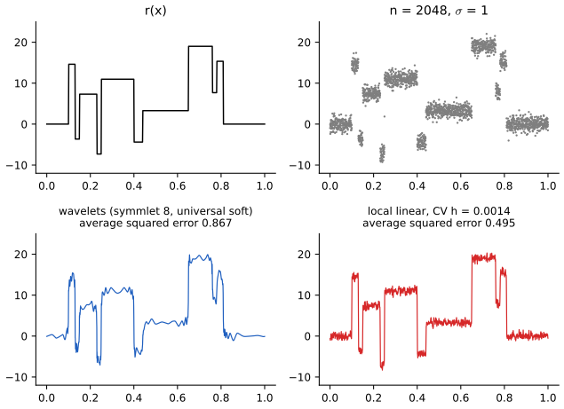
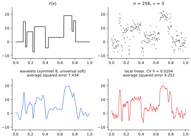
Example 9.39 (blocks). \(r(x)=3.655606\sum_{j=1}^{11}h_jK(x-t_j)\) with \(K(t)=(1+\sgn t)/2\), jump locations and heights
\[ t=(0.10,0.13,0.15,0.23,0.25,0.40,0.44,0.65,0.76,0.78,0.81), \] \[ h=(4,-5,3,-4,5,-4.2,2.1,4.3,-3.1,2.1,-4.2). \]The constant makes the standard deviation of \(r\) over \([0,1]\) equal to 7, so \(\sigma=1\) is a signal-to-noise ratio of 7 (checked numerically).
See also (companion courses): Probability and Statistical Inference, Algorithm 21.C (Haar wavelet regression) and Statistical Learning, Section 5.9 (wavelet smoothing).
9.5 Besov Spaces
pp. 211–214 Let \(\Delta_h^{(r)}f(x)=\sum_{k=0}^r\binom rk(-1)^kf(x+kh)\) be the \(r\)-th difference, \(w_{r,p}(f;t)=\sup_{|h|\le t}\|\Delta_h^{(r)}f\|_p\) the modulus of smoothness, and, for \(r-1\le\varsigma\le r\) (the book's convention),
\[ |f|^\varsigma_{p,q}=\Big(\int_0^\infty\big(h^{-\varsigma}w_{r,p}(f;h)\big)^q\frac{\d h}{h}\Big)^{1/q},\qquad|f|^\varsigma_{p,\infty}=\sup_{0<h<1}\frac{w_{r,p}(f;h)}{h^\varsigma}. \]The Besov ball \(B^\varsigma_{p,q}(c)\) is the set of \(f:[0,1]\to\R\) with \(\|f\|_p<\infty\) and \(|f|^\varsigma_{p,q}\le c\). Special cases: the Sobolev space \(W(m)\) is \(B^m_{2,2}\); \(B^m_{p,1}\subset W_p(m)\subset B^m_{p,\infty}\); the Hölder space of order \(s=m+\delta\) is \(B^s_{\infty,\infty}\); functions of bounded variation lie between \(B^1_{1,1}\) and \(B^1_{1,\infty}\). For sufficiently regular wavelets, \(f\in B^\varsigma_{p,q}(c)\) iff (up to constants) its coefficients satisfy
\[ \|\beta\|^\varsigma_{p,q}=\Bigg(\sum_{j\ge j_0}\Big(2^{j(\varsigma+1/2-1/p)}\Big(\sum_k|\beta_{jk}|^p\Big)^{1/p}\Big)^q\Bigg)^{1/q}\le c. \tag{9.40} \]Filling the gap 9.13: why smoothness is decay of wavelet coefficients (the case \(p=q=\infty\)) p. 213, (9.40)
Derivation
For \(p=q=\infty\), (9.40) says \(\sup_{j,k}2^{j(\varsigma+1/2)}|\beta_{jk}|\le c\). Here is the direction "Hölder implies decay", which is what the estimators use. Let \(f\) be Hölder of order \(\varsigma=m+\delta\) (\(m\) derivatives, \(|f^{(m)}(u)-f^{(m)}(v)|\le M|u-v|^\delta\)), and let \(\psi\) have support of length \(L\) and at least \(m+1\) vanishing moments. On the support \(I_{jk}\) of \(\psi_{jk}\), with \(x_0\) its left end, Taylor's formula gives \(f(x)=T(x)+R(x)\) with \(T\) a polynomial of degree \(m\) and \[|R(x)|\le\frac{M}{m!}|x-x_0|^{\varsigma}\le\frac{M}{m!}(L2^{-j})^\varsigma\]. The vanishing moments kill \(T\): \(\int T\psi_{jk}=0\). Hence
\[ |\beta_{jk}|=\Big|\int R\,\psi_{jk}\Big|\le\frac{M(L2^{-j})^\varsigma}{m!}\int|\psi_{jk}|=\frac{ML^\varsigma\|\psi\|_1}{m!}\,2^{-j\varsigma}\,2^{-j/2}, \]since \(\int|\psi_{jk}|=2^{-j/2}\|\psi\|_1\). So \(|\beta_{jk}|\le C2^{-j(\varsigma+1/2)}\). The converse (decay implies smoothness) needs the wavelet itself to be smoother than \(\varsigma\), and is where the hypothesis "\(r\) continuous derivatives" of Theorem 9.41 enters; see Härdle et al. (1998), Chapter 9.
Sobolev, \(p=q=2\). Then (9.40) is \(\sum_j2^{2j\varsigma}\sum_k\beta_{jk}^2\), the wavelet analogue of the Sobolev ellipsoid \(\sum_jj^{2m}\theta_j^2\) of Chapter 7: the energy at scale \(2^{-j}\) must decay like \(2^{-2j\varsigma}\).
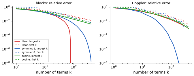
What \(p<2\) adds. For a function with a jump, about one coefficient per level is of size \(2^{-j/2}\) (the jump times \(\int|\psi_{jk}|\)), the rest are tiny. Then \(\big(\sum_k|\beta_{jk}|^p\big)^{1/p}\approx2^{-j/2}\) and the level-\(j\) term of (9.40) is \(2^{j(\varsigma-1/p)}\): bounded for \(\varsigma\le1/p\). With \(p=1\) and \(\varsigma=1\) the blocks function is in \(B^1_{1,\infty}\) (bounded variation), although it is not even continuous. Small \(p\) rewards sparsity, exactly as in Filling the gap 9.1. Numerically (Figure 9.S3), keeping the 77 largest Haar coefficients reproduces the 2048 samples of blocks exactly, while the first 77 leave 6 percent of the energy. ∎
Theorem 9.41 (Donoho and Johnstone 1995) pp. 213–214
Let \(\hr\) be the SureShrink estimator, with \(\psi\) having \(r\) vanishing moments and \(r\) continuous derivatives, \(r>\max\{1,\varsigma\}\). Let \(R_n(p,q,\varsigma,C)\) be the minimax risk over \(B^\varsigma_{p,q}(C)\). Then
\[ \sup_{r\in B^\varsigma_{p,q}(C)}\frac1n\E\sum_i(\hr(x_i)-r(x_i))^2\asymp R_n(p,q,\varsigma,C) \]for all \(1\le p,q\le\infty\), \(C\in(0,\infty)\) and \(\varsigma_0<\varsigma<r\), \(\varsigma_0=\max\{1/p,2(1/p-1/2)_+\}\). No linear estimator achieves the optimal rate over this range; the universal threshold attains it up to \(\log n\) factors.
Filling the gap 9.14: why thresholding beats every linear estimator when \(p<2\) p. 214
Derivation (the single-level calculation behind Theorem 9.41)
The full proof is long; its heart is one level of coefficients. At level \(j\) there are \(m=2^j\) coefficients observed with noise variance \(\epsilon^2=\sigma^2/n\), and by (9.40) they lie in the \(\ell_p\) ball \(\Theta=\{\theta\in\R^m:\sum|\theta_k|^p\le C^p\}\) with \(C=c\,2^{-j(\varsigma+1/2-1/p)}\).
Thresholding. For \(p\le2\) and any \(a\), \(\min(a^2,\epsilon^2)\le|a|^p\epsilon^{2-p}\) (if \(|a|\le\epsilon\), \(a^2=|a|^p|a|^{2-p}\le|a|^p\epsilon^{2-p}\); otherwise \(\epsilon^2\le|a|^p\epsilon^{2-p}\)). Hence the oracle risk satisfies \[\sup_\Theta\sum_k\min(\theta_k^2,\epsilon^2)\le\min(C^p\epsilon^{2-p},m\epsilon^2)\], and by the oracle inequality thresholding achieves this up to \(2\log n+1\).
Linear estimators. For this symmetric set the best linear estimator can be taken diagonal (Donoho, Liu and MacGibbon 1990). A diagonal estimator \(c_kX_k\) has risk \(\sum_k[c_k^2\epsilon^2+(1-c_k)^2\theta_k^2]\), which is linear in \(s_k=\theta_k^2\). Its worst case over \(\Theta\) is therefore its worst case over the convex hull of \(\{s:\sum s_k^{p/2}\le C^p\}\). That set contains the points \(C^2e_k\), and for \(p\le2\) it lies inside \(\{\sum s_k\le C^2\}\) (because \(\sum s_k\le(\sum s_k^{p/2})^{2/p}\)); so the hull is exactly the simplex \(\{\sum s_k\le C^2\}\), i.e. the \(\ell_2\) ball of radius \(C\) (the quadratic hull of \(\Theta\)). On the \(\ell_2\) ball the minimax linear risk is \(m\epsilon^2C^2/(m\epsilon^2+C^2)\asymp\min(C^2,m\epsilon^2)\) (Pinsker's calculation, Chapter 7).
The gap. When \(\epsilon\le C\le\sqrt m\,\epsilon\), thresholding pays \(C^p\epsilon^{2-p}\) and linear rules pay \(C^2\); their ratio is \((\epsilon/C)^{2-p}\), which tends to 0 when \(p<2\). Summing over levels with \(C=c2^{-j(\varsigma+1/2-1/p)}\) and balancing against \(m\epsilon^2=2^j\sigma^2/n\) gives the minimax rate \(n^{-2\varsigma/(2\varsigma+1)}\) for thresholding, while the linear rate is \(n^{-2\varsigma'/(2\varsigma'+1)}\) with \(\varsigma'=\varsigma-1/p+1/2<\varsigma\) (the smoothness of the quadratic hull). The condition \(\varsigma>\varsigma_0\) keeps the high-resolution tail negligible. ∎
9.6 Confidence Sets
pp. 214–215 Practical simultaneous bands for wavelet estimators are not available (a pointwise method is in Picard and Tribouley 2000); confidence balls are. For \(B^\varsigma_{p,q}\) let
\[ \gamma=\begin{cases}\varsigma&p\ge2\\\varsigma+\tfrac12-\tfrac1p&1\le p<2,\end{cases} \tag{9.42} \]let \(B(p,q,\gamma)\) be the corresponding set of coefficient sequences, and let \(\mu_n\) be the first \(n\) wavelet coefficients strung out as one vector, with \(\hat\mu\) their soft-thresholded estimates.
Theorem 9.43 (Genovese and Wasserman) pp. 214–215
Let
\[ D_n=\Big\{\mu_n:\sum_{\ell=1}^n(\hat\mu_\ell-\mu_\ell)^2\le s_n^2\Big\}, \tag{9.44} \] \[ s_n^2=\frac{\sqrt2\,\sigma^2z_\alpha}{\sqrt n}+S_n(\lambda), \tag{9.45} \] \[ S_n(\lambda)=\frac{\sigma^2}{n}2^{j_0}+\sum_{j=j_0}^JS_j(\lambda_j), \tag{9.46} \]with \(S_j\) the SURE of (9.38). Then for every \(\delta>0\), \[\lim_n\sup_{\mu\in\Delta(\delta)}|\P(\mu_n\in D_n)-(1-\alpha)|=0\] (9.47), where \[\Delta(\delta)=\bigcup\{B(p,q,\gamma):p,q\ge1,\gamma>\tfrac12+\delta\}\].
Filling the gap 9.15: where the radius (9.45) comes from p. 214
Derivation (heuristic, conditional on the threshold)
The ball is centred at \(\hat\mu\) and its squared radius estimates the loss \(L_n=\sum_\ell(\hat\mu_\ell-\mu_\ell)^2\) plus a margin. Fix the thresholds (the theorem's proof handles their data dependence by a uniformity argument over \(\lambda\)). The \(2^{j_0}\) unshrunk coefficients contribute \(\sigma^2/n\) each, hence the first term of (9.46); SURE estimates the expected loss of each level. The margin comes from the fluctuation of \(L_n-S_n\). Writing \(X_\ell=\mu_\ell+\epsilon Z_\ell\), \(\epsilon^2=\sigma^2/n\), the difference \(L_n-S_n\) is a sum of \(n\) independent mean-zero terms; for the coordinates that are killed (\(|X_\ell|\le\lambda\)) the term is \(\mu_\ell^2-(X_\ell^2-\epsilon^2)\)-like, for the kept ones \(\epsilon^2(Z_\ell^2-1)\)-like. When the signal is small relative to the noise (the condition \(\gamma>1/2\) ensures \(\sum\mu_\ell^2\) over high levels is negligible), the dominant part is \(\epsilon^2\sum_\ell(Z_\ell^2-1)\), with variance \(2n\epsilon^4=2\sigma^4/n\). By the central limit theorem \(L_n-S_n\approx N(0,2\sigma^4/n)\), so \(\P(L_n\le S_n+z_\alpha\sqrt2\,\sigma^2/\sqrt n)\to1-\alpha\), which is (9.45). The radius is of order \(n^{-1/4}\) at best, in agreement with the lower bound of Chapter 7 (Theorem 7.71, Normal Means and Minimax Theory): no confidence ball for \(\R^n\)-valued means can shrink faster. ∎
9.7 Boundary Corrections and Unequally Spaced Data
p. 215 Restricted to an interval, translated wavelets are no longer orthonormal near the ends. The simplest fix is to mirror the data about the endpoint (transform \((Y_1,\dots,Y_n,Y_n,\dots,Y_1)\) and keep the first half); the periodised transform used above instead wraps the data around. When the design is not equally spaced or \(n\) is not a power of 2, average the data in \(m=2^k\) equal bins, as small as possible subject to every bin being non-empty.
Filling the gap 9.16: what goes wrong at the boundary, and what mirroring fixes p. 215
Derivation
The periodised transform treats \(r\) as a function on the circle. If \(r(0)\neq r(1)\), the circle sees a jump of size \(|r(1)-r(0)|\) at the seam, and by Filling the gap 9.13 every level gets a coefficient of size about \(|r(1)-r(0)|2^{-j/2}\) there: an artificial jump that thresholding must either keep (spending noise) or kill (leaving a visible error near both ends). Mirroring makes the extended signal continuous across the seam (its derivative still flips sign, which costs only coefficients of size \(2^{-3j/2}\)). The variance of the mirrored coefficients is not exactly \(\sigma^2\) near the seam (each noise value appears twice), so the threshold is only approximately calibrated there. Blocks and Doppler both vanish at 0 and 1, so the periodic transform is harmless for them (on the sample of Figure 9.7 mirroring gives 1.01 against 0.87 for VisuShrink); adding the trend \(0.5x\) to the Doppler sample of Exercise 5 makes the ends differ, and then mirroring wins (SureShrink error 0.00158 against 0.00181).
Binning. If bin \(b\) holds \(n_b\) points, its average has mean \(\approx r\)(bin centre) and variance \(\sigma^2/n_b\): the coefficients are then heteroscedastic unless the \(n_b\) are about equal, and the threshold should be scaled accordingly. ∎
9.8 Overcomplete Dictionaries
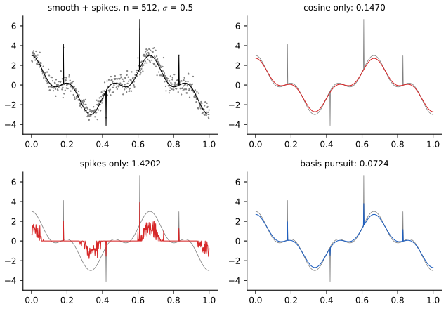
pp. 215–216 Let \(D\) be an \(n\times m\) matrix with \(m>n\) columns (a dictionary), e.g. the \(n\) cosine basis vectors next to the \(n\) "spikes" (unit vectors), so that \(r\) can be "smooth plus spikes". The columns can no longer be orthogonal. Basis pursuit (Chen, Donoho and Saunders 1998) chooses \(\beta\) to minimise
\[ \|Y-D\beta\|_2^2+\lambda\|\beta\|_1, \]which is the lasso (Tibshirani 1996) with the dictionary as design matrix.
Filling the gap 9.17: computing basis pursuit for a union of two orthonormal bases p. 216
Derivation
Let \(D=[C\ \ I]\), \(\beta=(a,b)\), with \(C\) orthogonal. The objective \(F(a,b)=\|Y-Ca-b\|^2+\lambda(\|a\|_1+\|b\|_1)\) is convex. Block updates are exact soft thresholds. For fixed \(b\), since \(C\) is orthogonal, \(\|Y-b-Ca\|^2=\|C^\T(Y-b)-a\|^2\), so minimising over \(a\) separates into scalar problems \(\min_a(z-a)^2+\lambda|a|\), whose solution is \(a=\sgn(z)(|z|-\lambda/2)_+\) (the subgradient condition \(2(a-z)+\lambda\,\partial|a|\ni0\)). So \(a\leftarrow\mathrm{soft}(C^\T(Y-b),\lambda/2)\) and likewise \(b\leftarrow\mathrm{soft}(Y-Ca,\lambda/2)\). Convergence. Each update does not increase \(F\); the non-smooth part is separable across the two blocks, so block coordinate descent converges to a minimiser (Tseng 2001), as in Sardy, Bruce and Tseng's block coordinate relaxation. The code's solution agrees with scikit-learn's lasso to \(10^{-4}\). Choice of \(\lambda\). With \(\lambda/2=\sigma\sqrt{2\log(2n)}\) (the universal threshold for \(2n\) coefficients), pure noise is killed in both bases with high probability, as in Theorem 9.33. The minimiser need not be unique when columns are dependent. ∎
See also (companion course): Statistical Learning, Section 3.4 (the lasso and its computation).
9.9 Other Adaptive Methods
pp. 216–220 Variable-bandwidth kernels, local polynomials with local bandwidths, and free-knot splines are also spatially adaptive. The book outlines the intersecting confidence intervals (ICI) rule of Goldenshluger and Nemirovski (1997). Let \(\hat r_h(x)=\sum_iY_i\ell_i(x,h)\) be a linear smoother, \(h_1<\dots<h_m\) a grid of bandwidths, \(\hat r_j=\hat r_{h_j}(x)\), and \(\sigma\) known. Then \(\hat r_j=\sum_ir(x_i)\ell_i(x,h_j)+\xi_j\) with \(\xi_j\sim N(0,s_j^2)\), \(s_j=\sigma\|\ell(x,h_j)\|\). Let \(\rho_j=\kappa s_j\) with \(\kappa>\sqrt{2\log n}\), form the intervals \(D_j=\hat r_j\pm2\rho_j\), and set
\[ \hat r(x)=\hat r_{j_+}(x), \tag{9.48} \] \[ j_+=\max\Big\{k:\bigcap_{j=1}^kD_j\neq\emptyset\Big\}. \tag{9.49} \]Filling the gap 9.18: the ICI oracle bound, with the monotonicity the right way round pp. 217–218
Proof
Setting. With bandwidths increasing in \(j\), the standard deviation \(s_j\) decreases in \(j\) (more points are averaged) and the bias \(b_j=|\E\hat r_j-r(x)|\) increases in \(j\), as it does for most smoothers and most \(r\). (The book states the opposite monotonicity, which would break the last step below; see Notes on the book.) Let \(j^*=\max\{j:b_j\le\rho_j\}\), the bandwidth balancing bias and noise; \(\rho_{j^*}\) is the oracle accuracy.
The good event. Let \(G=\{|\xi_j|\le\rho_j\text{ for all }j\}\). By a union bound and Mills' inequality, with \(m\le n\) bandwidths,
\[ \P(G^c)\le m\,\P(|Z|>\kappa)\le n\sqrt{\frac2\pi}\frac{e^{-\kappa^2/2}}{\kappa}\le\sqrt{\frac2\pi}\frac{1}{\kappa}\quad\text{if }\kappa\ge\sqrt{2\log n}, \]which tends to 0. On \(G\):
(i) For \(j\le j^*\), \[|\hat r_j-r(x)|\le b_j+|\xi_j|\le b_j+\rho_j\le b_{j^*}+\rho_j\le\rho_{j^*}+\rho_j\le2\rho_j\] (using \(b_j\le b_{j^*}\le\rho_{j^*}\le\rho_j\)). So \(r(x)\in D_j\) for every \(j\le j^*\): these intervals intersect, and \(j_+\ge j^*\).
(ii) By definition of \(j_+\), \(D_1\cap\dots\cap D_{j_+}\neq\emptyset\); in particular \(D_{j_+}\) and \(D_{j^*}\) share a point \(p\). Then \(|\hat r_{j_+}-p|\le2\rho_{j_+}\), \(|p-\hat r_{j^*}|\le2\rho_{j^*}\), and \(|\hat r_{j^*}-r(x)|\le2\rho_{j^*}\) by (i). Since \(j_+\ge j^*\) and \(\rho\) is decreasing, \(\rho_{j_+}\le\rho_{j^*}\), so
\[ |\hat r(x)-r(x)|\le2\rho_{j_+}+2\rho_{j^*}+2\rho_{j^*}\le6\rho_{j^*}. \]So with probability tending to one the ICI estimate is within a constant times the oracle accuracy, without knowing the bias. The price is the factor \(\kappa\approx\sqrt{2\log n}\) inside \(\rho\): a logarithmic loss, which Lepskii (1991) showed to be unavoidable for pointwise adaptation. On the Doppler sample at \(x=0.6\), \(|\hat r-r|=0.145\le6\rho_{j^*}=0.217\) (Figure 9.9). ∎
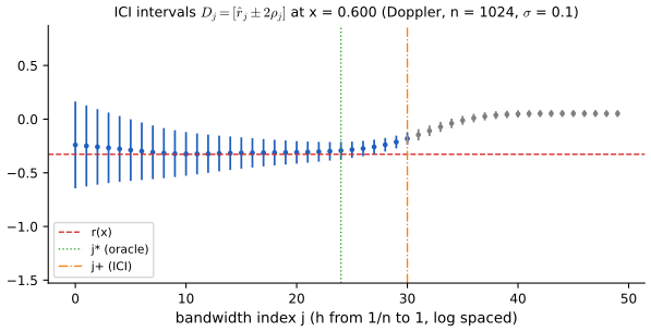
A concrete implementation fits a local polynomial of degree \(m\) on intervals \(\Delta\ni x\), \(\hat r_\Delta(x)=\sum_i\alpha_\Delta(x_i,x)Y_i\), with \(|\alpha_\Delta(x_i)|\le c_m/N_\Delta\) (\(N_\Delta\) points in \(\Delta\)), forms the intervals \(D_\Delta=\hat r_\Delta\pm2\kappa s_\Delta\) with \(s_\Delta^2=\sum_i\alpha_\Delta^2(x_i)\), with \(\kappa_n\) a constant times \(\sigma\sqrt{(m+2)\log n}\), and takes the largest \(\Delta\) such that all \(D_\delta\), \(\delta\subset\Delta\), intersect. Suppose \(r\) has \(\ell\) derivatives on \(\Delta_0=[x-\delta_0,x+\delta_0]\) with \((\int_{\Delta_0}|r^{(\ell)}|^p)^{1/p}\le L\), \(\ell\le m+1\), \(p\ell>1\).
Theorem 9.50 (Goldenshluger and Nemirovski 1997) p. 219
\[ \big(\E|\hat r(x)-r(x)|^2\big)^{1/2}\le CB_n, \tag{9.51} \] \[ B_n=\Big(\frac{\log n}{n}\Big)^{(p\ell-1)/(2p\ell+p-2)}L^{p/(2p\ell+p-2)}+\Big(\frac{\log n}{n\delta_0}\Big)^{1/2}, \tag{9.52} \]with \(C\) depending only on \(m\). Up to the logarithm (unavoidable, Lepskii 1991) this is the best possible rate, achieved without knowing \(p\), \(\ell\) or \(L\).
Filling the gap 9.19: where the exponents of (9.52) come from p. 219
Derivation
By Filling the gap 9.18 the ICI estimate is within a constant of the best interval \(\Delta=[x-h,x+h]\subset\Delta_0\), up to \(\kappa\asymp\sqrt{\log n}\). For a symmetric window of half-width \(h\), \(N_\Delta\asymp nh\) and \(s_\Delta\asymp\sigma/\sqrt{nh}\) (from \(|\alpha|\le c_m/N_\Delta\)), so the stochastic term is \(\asymp\sqrt{\log n/(nh)}\). Bias. A local polynomial of degree \(m\ge\ell-1\) reproduces polynomials of degree \(\ell-1\), so the bias is \(\sum_i\alpha_\Delta(x_i)R(x_i)\), with \(R\) the Taylor remainder of order \(\ell\) at \(x\): \[R(u)=\frac1{(\ell-1)!}\int_x^u(u-t)^{\ell-1}r^{(\ell)}(t)\,\d t\]. By Hölder's inequality with exponents \(p\) and \(p/(p-1)\), \[|R(u)|\le\frac{1}{(\ell-1)!}|u-x|^{\ell-1}|u-x|^{1-1/p}L=C L h^{\ell-1/p}\] for \(|u-x|\le h\). Since \(\sum|\alpha_\Delta|\le c_m\), the bias is at most \(CLh^{\ell-1/p}\) (this needs \(p\ell>1\)). Balance. \(Lh^{\ell-1/p}=\sqrt{\log n/(nh)}\) gives \(h^{2\ell-2/p+1}=\log n/(nL^2)\), i.e. \(h=(\log n/(nL^2))^{p/(2p\ell+p-2)}\), and the error \[Lh^{\ell-1/p}=(\log n/n)^{(p\ell-1)/(2p\ell+p-2)}L^{p/(2p\ell+p-2)}\]: the first term of (9.52). If the balancing \(h\) exceeds \(\delta_0\), the window is capped at \(\delta_0\) and the error is the noise level \(\sqrt{\log n/(n\delta_0)}\): the second term. For \(p=\infty\) the rate is \((\log n/n)^{\ell/(2\ell+1)}\), the familiar pointwise rate for \(\ell\) derivatives. ∎
Lepski's method (a version of Lepski, Mammen and Spokoiny 1997). With bandwidths \(h_j=a^{-j}\) (they use \(a=1.02\)), take the largest \(h\) for which reducing the bandwidth does not change the fit significantly: \[\hat h=\max\{h:|\hat r_h(x)-\hat r_\eta(x)|\le\psi(h,\eta)\text{ for all }\eta<h\}\], with \(\psi(h,\eta)=D\sigma\sqrt{(1+\log(1/\eta))/(n\eta)}\), a multiple of the standard deviation of the smaller-bandwidth estimate inflated by a logarithm. The code uses \(\psi=\Gamma s_\eta\) with a tuning constant \(\Gamma\).
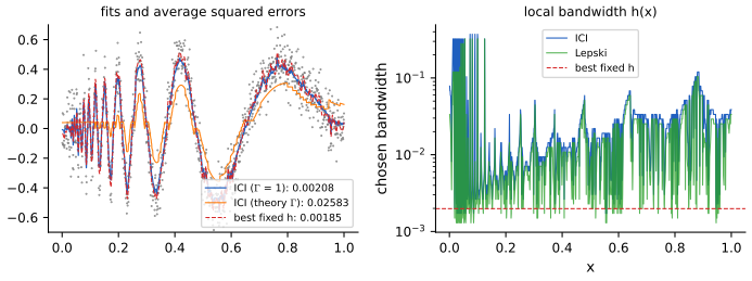
See also: Chapter 5 of this course, Section 5.4, where Doppler data defeat a single cross-validated bandwidth (demo).
9.10 Do Adaptive Methods Work?
pp. 220–221 Let \(r\) be piecewise polynomial of degree \(D\) on intervals \(A_1,\dots,A_L\) partitioning \([0,1]\). With known breakpoints, least squares on each piece is a parametric problem with risk \(O(1/n)\). With unknown breakpoints, a kernel estimator has risk no better than order \(n^{-1/2}\) in general, while Donoho and Johnstone show that the wavelet method achieves \(O(\log n/n)\) (for the ideal risk; the universal threshold gets within one more \(\log n\) by (9.37)). But for inference the picture is different: since \((r(x_1),\dots,r(x_n))\) can still be any vector in \(\R^n\), Theorem 7.71 says no confidence ball can shrink faster than \(n^{-1/4}\). Fast estimation, slow inference.
Filling the gap 9.20: \(n^{-1/2}\) for kernels and \(\log n/n\) for wavelets at a jump p. 220
Derivation
Kernels. Let \(r\) jump by \(a\neq0\) at \(t\). For any kernel estimator with bandwidth \(h\), on the set \(\{x:|x-t|\le h/2\}\) of length \(h\) the window straddles the jump with a fixed fraction of its weight on each side, so the bias is at least \(c|a|\) there (for a symmetric kernel, at \(x=t\) the estimate is near the average of the two levels). The integrated squared bias is therefore \(\ge c^2a^2h\), the integrated variance \(\asymp\sigma^2/(nh)\), and \(\inf_h(c^2a^2h+\sigma^2/(nh))\asymp|a|\sigma n^{-1/2}\), attained at \(h\asymp n^{-1/2}\). Local polynomials of any degree have the same problem.
Wavelets. Take a wavelet with more than \(D\) vanishing moments and support length \(S\). A detail coefficient is nonzero only if the support of \(\psi_{jk}\) contains a breakpoint, i.e. for at most \(S\) values of \(k\) per breakpoint and level, so at most \(LS\log_2n\) of the \(n\) coefficients are nonzero. The oracle risk is then at most \((LS\log_2n)\,\sigma^2/n\), i.e. \(O(\log n/n)\), and (9.37) gives \(O(\log^2n/n)\) for VisuShrink. Figure 9.S8 shows the empirical rates on blocks: from \(n=256\) to 4096 the risk of the best fixed-bandwidth local linear fit falls by a factor of 2.3 (slope about \(-0.30\) on the log scale), Haar VisuShrink by 5.7 (slope \(-0.63\)) and SureShrink by 4.2. ∎
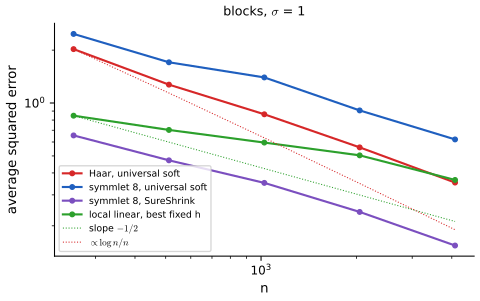
So: when accurate function estimates are needed and the noise is low, adaptive estimators are very effective; for a standard nonparametric regression problem where confidence statements matter, they do not do much better than a fixed-bandwidth local regression. Exercise 5 below quantifies this on Doppler data.
9.11 Bibliographic Remarks
p. 221 Ogden (1997) is an introduction to wavelets in statistics, Härdle, Kerkyacharian, Picard and Tsybakov (1998) an advanced treatment, Daubechies (1992) the mathematical source. The statistical theory is in Donoho and Johnstone (1994, 1995, 1998) and Donoho, Johnstone, Kerkyacharian and Picard (1995); the confidence sets are from Genovese and Wasserman (2005).
9.12 Appendix
pp. 221–223 Localisation. For \(f\) with \(\|f\|=1\) define its centre \(\bar x=\int x|f|^2\) and radius \(\Delta_f=(\int(x-\bar x)^2|f(x)|^2\d x)^{1/2}\) (normalising by \(\|f\|\) in general), and likewise \(\Delta_{f^*}\) for \(f^*\). A cosine is perfectly localised in frequency but not at all in space; a wavelet is localised in both, within the following limit.
Theorem 9.53 (Heisenberg's uncertainty relation) p. 222
\[ \Delta_f\,\Delta_{f^*}\ge\frac12, \tag{9.54} \]with equality when \(f\) is a Normal density.
Filling the gap 9.21: proof of (9.54) p. 222
Proof
Translating \(f\) or modulating it by \(e^{i\omega x}\) changes neither radius, so assume both centres are 0; take \(f\) smooth and rapidly decreasing (the general case follows by density), real for simplicity. Plancherel for (9.1) reads \(\int|f^*|^2=2\pi\int|f|^2\), and \((f')^*(t)=it\,f^*(t)\), so \(\int t^2|f^*(t)|^2\d t=2\pi\int|f'|^2\). Hence \[\Delta_{f^*}^2=\int t^2|f^*|^2/\int|f^*|^2=\int|f'|^2/\int|f|^2\]. Integrating by parts, \(\int f^2=\big[xf^2\big]-\int x\,2ff'=-2\int xff'\), and by Cauchy–Schwarz \(\big(\int f^2\big)^2\le4\int x^2f^2\int f'^2\). Dividing by \(\big(\int f^2\big)^2\): \(1\le4\Delta_f^2\Delta_{f^*}^2\). Equality in Cauchy–Schwarz requires \(f'=-cxf\), i.e. \(f\propto e^{-cx^2/2}\): a Normal density. Numerically: the product is 0.500 for a Gaussian and 0.54 for the triangle function \((1-|x|)_+\). ∎
Fast computation. From \(\phi_{jk}(x)=\sum_r\ell_{r-2k}\phi_{j+1,r}(x)\) and the analogous identity for \(\psi_{jk}\), integrating against \(f\) gives the cascade equations
\[ \alpha_{jk}=\sum_r\ell_{r-2k}\,\alpha_{j+1,r}, \tag{9.55} \] \[ \beta_{jk}=\sum_r(-1)^{r+1}\ell_{-r+2k+1}\,\alpha_{j+1,r}. \tag{9.56} \]In filter language, \((Af)_k=\sum_ra_{r-2k}f_r\) (9.57); with the low-pass filter \(L\) (coefficients \(\ell_k\)) and the high-pass filter \(H\) (coefficients \(h_k=(-1)^{k+1}\ell_{1-k}\)), \(\alpha_{j-1,\cdot}=L\alpha_{j,\cdot}\), \(\alpha_{j-m,\cdot}=L^m\alpha_{j,\cdot}\) (9.58), \(\beta_{j-1,\cdot}=H\alpha_{j,\cdot}\) and \(\beta_{j-m,\cdot}=HL^{m-1}\alpha_{j,\cdot}\) (9.59). Starting from finest-level scaling coefficients computed from the data, this is the discrete wavelet transform, \(O(n)\) operations. Figure 9.10, a diagram of this pyramid, is not reproduced.
Filling the gap 9.22: the cascade equations, and why the transform is orthogonal and \(O(n)\) pp. 222–223
Derivation
(9.55). By (9.16), \(\phi(y)=\sum_r\ell_r\sqrt2\,\phi(2y-r)\). Put \(y=2^jx-k\) and multiply by \(2^{j/2}\): \[\phi_{jk}(x)=\sum_r\ell_r2^{(j+1)/2}\phi(2^{j+1}x-2k-r)=\sum_r\ell_r\phi_{j+1,r+2k}(x)=\sum_r\ell_{r-2k}\phi_{j+1,r}(x)\] (re-indexing \(r+2k\to r\); the book's middle expression has \(\ell+2k\) for \(r+2k\)). Take the inner product with \(f\). (9.56) follows the same way from \(\psi(y)=\sqrt2\sum_r(-1)^{r+1}\ell_{1-r}\phi(2y-r)\): \[\psi_{jk}=\sum_r(-1)^{r+1}\ell_{1-r}\phi_{j+1,r+2k}=\sum_r(-1)^{r+1}\ell_{1-r+2k}\phi_{j+1,r}\] (since \((-1)^{r-2k}=(-1)^r\)).
Orthogonality. One step maps \(\alpha_{j+1,\cdot}\) (length \(2^{j+1}\), periodised) to \((\alpha_{j,\cdot},\beta_{j,\cdot})\). Its rows are the even shifts of \(\ell\) and of \(h\); they are orthonormal because \(\sum_k\ell_k\ell_{k+2m}=\delta_{m0}\), \(\sum_kh_kh_{k+2m}=\delta_{m0}\) and \(\sum_k\ell_kh_{k+2m}=0\), the coefficient forms of the unitarity of Filling the gap 9.6. A square matrix with orthonormal rows is orthogonal, and the full transform is a product of such steps. Cost. A step on a vector of length \(N\) costs \(N\times\)(filter length) operations, and the lengths halve, so the total is at most \(2n\times\)(filter length) \(=O(n)\). The Haar case in full: Probability and Statistical Inference, Filling the gap 21.17. ∎
Notes on the book
The book's website has no errata list. Each point below gives the evidence: a derivation in these notes or a computation.
Page 203, Definition 9.11: orthonormal translates are needed
Lemma 9.14 asserts that \(\{\phi_{jk}\}_k\) is an orthonormal basis of \(V_j\), which requires \(\{\phi(\cdot-k)\}\) to be orthonormal; Definition 9.11 asks only for nesting and density. The hat function \(\phi(x)=(1-|x-1|)_+\) generates nested, dense spaces (continuous piecewise linear functions with dyadic knots) but \(\langle\phi,\phi(\cdot-1)\rangle=1/6\neq0\). The standard definition includes orthonormality (or a Riesz basis) of the translates. See Filling the gap 9.3.
Page 204: one factor too many in the infinite product
Iterating (9.17) gives \(\phi^*(t)=\prod_{k=1}^\infty m_0(t/2^k)\,\phi^*(0)\); the text has an extra \(m_0(t/2)\) in front of the product (it would square the first factor). (9.20) is correct. See Filling the gap 9.4.
Page 210, (9.37): the lower bound \(R_n^*\le R(\hat\theta,\theta)\) is false
The soft-threshold estimator is not a "kill it or keep it" estimator, and its risk can be below the oracle risk. Take \(\theta_i=\sigma/\sqrt n\) for all \(i\) and \(n=1024\): \(R_n^*=\sigma^2\), while the exact risk (Exercise 8) is \(n\cdot\frac{\sigma^2}{n}r(1)=0.99859\,\sigma^2\) with \(\lambda=\sqrt{2\log1024}\). The derivation in Filling the gap 9.11 shows why: \(r(\theta)=r(0)+\int_0^\theta2u\,\P_u(|X|\le\lambda)\d u\) can be slightly below \(\theta^2\). The upper bound, which is Donoho and Johnstone's theorem, is correct. The theorem also writes \(Y_i\) for the data and \(X_i\) inside the estimator.
Pages 210–211, SureShrink: \(n_j=2^j\), and the upper limit uses \(\sigma/\sqrt n\)
With levels indexed as in (9.26), level \(j\) has \(2^j\) coefficients, not \(2^{j-1}\). The noise standard deviation of each \(D_{jk}\) is \(\sigma/\sqrt n\) (9.28), so the universal limit for level \(j\) is \((\sigma/\sqrt n)\sqrt{2\log n_j}\), not \((\sigma/\sqrt{n_j})\sqrt{2\log n_j}\); also the \(\hb_{jk}\) inside (9.38) must be the empirical \(D_{jk}\) (SURE is a function of the data). See Filling the gap 9.12.
Page 211, Example 9.39: the wavelet fit is not better in squared error
On a sample like the book's (\(n=2048\), \(\sigma=1\)), VisuShrink with the symmlet 8 has average squared error 0.867 against 0.495 for cross-validated local linear regression; on three further samples it is 0.86, 0.97 and 0.92. The wavelet fit looks cleaner between the jumps, which is probably what the book judged by eye; the universal soft threshold pays a bias of \(\lambda\) on every kept coefficient. Hard thresholding (0.30 to 0.38 on the same four samples) and SureShrink (0.22 to 0.26) do much better; on the sample of the figure they give 0.320 and 0.232, against 0.495 for local linear regression. See Figure 9.7.
Page 214, Theorem 9.43: the threshold and a stray \(\d x\)
The theorem uses "the universal soft threshold \(\lambda=\sigma\sqrt{\log n/n}\)", which differs from (9.32) by a factor \(\sqrt2\); (9.44) contains a stray \(\d x\) in a finite sum, and (9.46) writes \(S(\lambda_j)\) for the \(S_j(\lambda_j)\) defined just after it.
Pages 217–218, ICI: the monotonicity is reversed
With bandwidths increasing in \(j\) (the book's example \(h_j=j/n\)), the standard deviation \(s_j\) decreases and the bias increases in \(j\); the book says the opposite. With its stated direction, \(j_+\ge j^*\) would give \(\rho_{j_+}\ge\rho_{j^*}\) and the final step \(2\rho_{j_+}+4\rho_{j^*}\le6\rho_{j^*}\) would fail. Also, \(D_{j_+}\cap D_{j^*}\neq\emptyset\) follows from the definition of \(j_+\), not of \(j^*\). For the Nadaraya–Watson estimator on the Doppler design, \(s_j\) is decreasing in \(h_j\) at every point (checked numerically). See Filling the gap 9.18.
Page 222: \(\phi_{j+1,\ell+2k}\) should be \(\phi_{j+1,r+2k}\)
In the derivation of the cascade equations the summation index is \(r\). See Filling the gap 9.22.
Page 224, Exercise 6(a): the sign of \(\hb_{jk}\)
With the mother wavelet (9.5), equal to \(-1\) on the left half, \[\hb_{jk}=\frac{2^{j/2}}n\big(N_{(2k+1)/2^{j+1},(2k+2)/2^{j+1}}-N_{2k/2^{j+1},(2k+1)/2^{j+1}}\big)\]: right count minus left count. The printed formula (left minus right) corresponds to the opposite sign convention for \(\psi\). Checked against \(\frac1n\sum_i\psi_{jk}(X_i)\) on the geyser data.
9.13 Exercises
All 9 exercises of Chapter 9 (pp. 223–225), restated in my own words, with complete solutions (hidden). Computational solutions use the chapter's code.
Exercise 9.1. Show that the Haar scaling coefficients are \(\ell_0=\ell_1=2^{-1/2}\) and \(\ell_k=0\) otherwise.
Solution
\(\ell_k=\int\phi(x)\sqrt2\,\phi(2x-k)\,\d x\). The second factor is \(\sqrt2\) on \([k/2,(k+1)/2)\); this interval lies in \([0,1)\) iff \(k\in\{0,1\}\), where \(\ell_k=\sqrt2\cdot\frac12=2^{-1/2}\); for other \(k\) the supports are disjoint and \(\ell_k=0\). Check: \[\phi(x)=\phi(2x)+\phi(2x-1)=2^{-1/2}\phi_{10}(x)+2^{-1/2}\phi_{11}(x)\].
Exercise 9.2. Prove Theorem 9.6.
Solution
See Filling the gap 9.2: orthonormality from the nested-or-disjoint structure of dyadic intervals and \(\int\psi_{jk}=0\); completeness because the first \(2^J\) functions span the dyadic step functions \(V_J\), whose union is dense in \(\Ltwo(0,1)\).
Exercise 9.3. Prove that the Haar wavelets form an MRA (Example 9.15).
Solution
See Filling the gap 9.3: the integer translates of the indicator of \([0,1)\) are orthonormal, \(V_j\) is the space of square-integrable functions constant on dyadic intervals of length \(2^{-j}\), these spaces are nested, and their union is dense because compactly supported continuous functions are uniform limits of their dyadic averages.
Exercise 9.4. Prove equation (9.17).
Solution
See Filling the gap 9.4: the transform of \(\sqrt2\phi(2x-k)\) is \(2^{-1/2}e^{-ikt/2}\phi^*(t/2)\); summing with weights \(\ell_k\) gives \(\phi^*(t)=m_0(t/2)\phi^*(t/2)\).
Exercise 9.5. Simulate \(Y_i=r(i/n)+\sigma\epsilon_i\) for the Doppler function, \(n=1024\). (a) Fit with wavelets using (i) James–Stein at each level, (ii) universal shrinkage, (iii) SureShrink, for \(\sigma=0.01,0.1,1\), and compare with REACT and with local linear regression. (b) Repeat with outliers: \(\epsilon_i\sim0.95N(0,1)+0.05N(0,4)\).
Solution
Method. Symmlet 8, periodic transform down to \(j_0=5\), \(\hs\) from the MAD; James–Stein: \(\big(1-(n_j-2)/\sum_kd_{jk}^2\big)_+\) on the standardised coefficients of each level; universal: soft at \(\hs\sqrt{2\log n}\); SureShrink: (9.38) per level. REACT: the orthonormal cosine (DCT-II) basis with the nested subset chosen by SURE (Chapter 8). Local linear: tricube kernel, bandwidth by leave-one-out cross-validation over 30 values. 10 replications; \(N(0,4)\) read as variance 4. Average squared errors \(\frac1n\sum(\hr(x_i)-r(x_i))^2\):
noise \(\sigma\) JS per level universal SureShrink REACT local linear Gaussian 0.01 6.9e-5 8.3e-5 2.7e-5 7.4e-5 1.13e-4 Gaussian 0.1 2.01e-3 2.78e-3 1.49e-3 2.68e-3 2.13e-3 Gaussian 1 0.0506 0.0428 0.0636 0.0380 0.0322 contaminated 0.01 7.9e-5 1.00e-4 3.1e-5 9.0e-5 1.19e-4 contaminated 0.1 2.26e-3 3.01e-3 1.79e-3 2.92e-3 2.30e-3 contaminated 1 0.0604 0.0466 0.0866 0.0439 0.0326 Conclusions. At low noise SureShrink is best, by a factor of 4 over local linear regression at \(\sigma=0.01\) and 1.4 at \(\sigma=0.1\) (the fast oscillations near 0 need fine-scale coefficients only there). At \(\sigma=1\) the ordering reverses: the fine structure is invisible, SURE is noisy and keeps too much, and the single cross-validated bandwidth wins; the universal threshold, being conservative, is the best wavelet rule there. The contamination (5 percent of errors with twice the standard deviation) inflates every error, by 1 to 36 percent; the MAD estimate of \(\sigma\) is robust, so the thresholds are hardly affected, but the outliers themselves pass through as noise. This is Section 9.10 in numbers. Figure 9.S4 shows one sample at \(\sigma=0.1\).
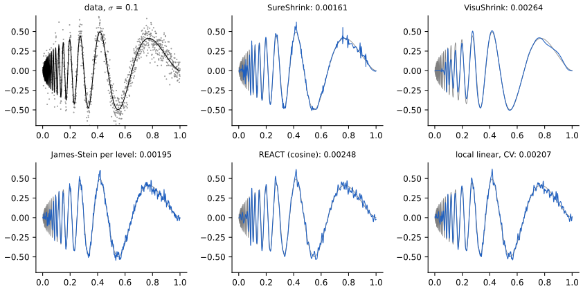
Figure 9.S4. Exercise 5: one Doppler sample (\(\sigma=0.1\)) fitted five ways, with the average squared error of each. Download: PDF · SVG Exercise 9.6. A wavelet histogram. For \(X_1,\dots,X_n\sim f\) on \([0,1]\) write \(f\approx\phi+\sum_{j\le J}\sum_k\beta_{jk}\psi_{jk}\) with Haar wavelets and \(J\approx\log_2(n+1)\); \(\hb_{jk}=\frac1n\sum_i\psi_{jk}(X_i)\) is unbiased for \(\beta_{jk}=\E\psi_{jk}(X)\). (a) Express \(\hb_{jk}\) through the counts \(N_{x,y}=\#\{i:x\le X_i<y\}\). (b) Show \(\hb_{jk}\approx N(\beta_{jk},\sigma_{jk}^2)\) and find \(\sigma_{jk}\). (c) With \(\sigma_{jk}\) known, find the per-level shrinkage \(a_j\) in \(\tilde\beta_{jk}=a_j\hb_{jk}\) that minimises SURE. (d) Estimate \(\sigma_{jk}\), apply to the geyser durations and compare with the histogram whose binwidth is chosen by cross-validation. (e) Since \(\hb_{jk}\) is \(2^{j/2}\) times a difference of two sample proportions, keep only the coefficients for which a test of \(\beta_{jk}=0\) rejects at level \(\alpha\); try several \(\alpha\).
Solution
(a) \(\psi_{jk}=2^{j/2}\) on the right half \([(2k+1)/2^{j+1},(2k+2)/2^{j+1})\) of its support and \(-2^{j/2}\) on the left half, so \[\hb_{jk}=\frac{2^{j/2}}n\big(N_{\text{right}}-N_{\text{left}}\big)\] (the book's display has the opposite sign; Notes on the book).
(b) \(\hb_{jk}\) is an average of the i.i.d. bounded variables \(\psi_{jk}(X_i)\), so by the central limit theorem it is approximately normal with mean \(\beta_{jk}\) and variance \(\sigma_{jk}^2=\Var\psi_{jk}(X)/n=(2^jp_{jk}-\beta_{jk}^2)/n\), where \(p_{jk}=\P(X\in\text{support of }\psi_{jk})\), because \(\psi_{jk}^2=2^j\) on its support. (Checked by simulation from a Beta(2,5) density.)
(c) \(\E(a\hb-\beta)^2=a^2\sigma^2+(1-a)^2\beta^2\), and \(\hb^2-\sigma^2\) is unbiased for \(\beta^2\), so SURE for level \(j\) is \(\sum_k[a^2\sigma_{jk}^2+(1-a)^2(\hb_{jk}^2-\sigma_{jk}^2)]\). Setting the derivative to zero: \(a\sum\sigma_{jk}^2=(1-a)\sum(\hb_{jk}^2-\sigma_{jk}^2)\), i.e. \(a_j=1-\sum_k\sigma_{jk}^2/\sum_k\hb_{jk}^2\), truncated to \([0,1]\).
(d) Plug in \(\hat\sigma_{jk}^2=(2^j\hat p_{jk}-\hb_{jk}^2)/n\) with \(\hat p_{jk}\) the sample proportion. Geyser durations (272 eruptions, rescaled from \([1.5,5.5]\) minutes to \([0,1]\)), \(J=8\): the factors are \(a_j=0.94,0.97,0.95,0.90,0.63,0.09,0,0.42\) for \(j=0,\dots,7\). The finest level is not shrunk to zero because the durations are recorded with many ties (126 distinct values; e.g. 1.75 minutes six times), which creates genuine fine-scale structure in the empirical distribution. The cross-validated histogram (score of Chapter 6, Density Estimation) uses 40 bins. Both show the two modes near 2 and 4.4 minutes; the wavelet estimate is spikier (Figure 9.S5, left) and, like any orthogonal series estimate, can dip slightly below zero.
(e) Under \(\beta_{jk}=0\) the two half-interval probabilities are equal, so, conditionally on \(N_L+N_R\), \(N_R\sim\mathrm{Bin}(N_L+N_R,1/2)\); use \(z=(N_R-N_L)/\sqrt{N_L+N_R}\) and keep \(\hb_{jk}\) if \(|z|>z_{\alpha/2}\). The number of coefficients kept is 7 (\(\alpha=0.01\)), 20 (\(\alpha=0.05\)) and 61 (\(\alpha=0.2\)): small \(\alpha\) gives a coarse two-bump staircase, large \(\alpha\) a noisy one (Figure 9.S5, right). With some 250 tests, \(\alpha=0.01\) to 0.05 is the sensible range (about 2.5 to 12 false inclusions expected at most).
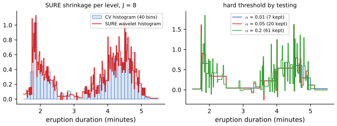
Figure 9.S5. Exercise 6: Haar wavelet histograms of the 272 geyser eruption durations. Left: SURE shrinkage per level against the cross-validated histogram. Right: hard thresholding by testing at three levels. Download: PDF · SVG Exercise 9.7. (a) Show that the oracle risk (9.35) is \(R_n^*=\sum_i(\sigma^2/n\wedge\theta_i^2)\). (b) Compare \(R_n^*\) with the Pinsker bound of Theorem 7.28; for which \(\theta\) is \(R_n^*\) smaller?
Solution
(a) See Filling the gap 9.11: the risk of \(\hat\theta_S\) is \(\sum_{i\in S}\sigma^2/n+\sum_{i\notin S}\theta_i^2\), minimised coordinate by coordinate.
(b) Theorem 7.28 (Chapter 7, Normal Means and Minimax Theory) gives the minimax risk over the ball \(\sum\theta_i^2\le c^2\) as \(R_P=\sigma^2c^2/(\sigma^2+c^2)\). Compare at \(c=\|\theta\|\). Always \[R_n^*\le\min(\|\theta\|^2,n\cdot\sigma^2/n)=\min(c^2,\sigma^2)\le2\sigma^2c^2/(\sigma^2+c^2)=2R_P\], using \(\min(a,b)\le2ab/(a+b)\): the oracle is never worse than twice Pinsker. Spread-out \(\theta\) (all \(\theta_i^2=c^2/n\)): \(R_n^*=\min(c^2,\sigma^2)\ge R_P\), so Pinsker's (linear) bound is smaller, by at most a factor 2. Sparse \(\theta\) (\(k\) coordinates of size at least \(\sigma/\sqrt n\), the rest 0): \(R_n^*=k\sigma^2/n\), while \(R_P\) depends only on \(c\) and is of order \(\min(c^2,\sigma^2)\); e.g. \(k=3\), \(\theta_i=1\), \(\sigma=1\), \(n=1000\): \(R_n^*=0.003\) against \(R_P=0.75\). So \(R_n^*<R_P\) exactly for vectors whose energy is concentrated on few coordinates, which is the situation wavelets create.
Exercise 9.8. Find exact expressions for the risks of the hard and soft threshold rules (\(\sigma\) known).
Solution
Take unit noise, \(X\sim N(\theta,1)\), threshold \(\lambda\); for noise \(\epsilon\) use \(\epsilon^2r(\theta/\epsilon,\lambda/\epsilon)\). Write \(a=\lambda-\theta\), \(b=-\lambda-\theta\), \(Z=X-\theta\), and use \(\int_u^vz\phi=\phi(u)-\phi(v)\), \(\int_u^vz^2\phi=u\phi(u)-v\phi(v)+\Phi(v)-\Phi(u)\).
Hard. \(t(X)-\theta=-\theta\) on \(\{|X|<\lambda\}=\{b<Z<a\}\) and \(=Z\) otherwise. So \[ r_H=\theta^2[\Phi(a)-\Phi(b)]+\E[Z^2;Z\ge a]+\E[Z^2;Z\le b] \], and with the identities,
\[ r_H(\theta,\lambda)=\theta^2\big[\Phi(\lambda-\theta)-\Phi(-\lambda-\theta)\big]+\Phib(\lambda-\theta)+\Phib(\lambda+\theta)+(\lambda-\theta)\phi(\lambda-\theta)+(\lambda+\theta)\phi(\lambda+\theta). \]Soft. \(t(X)-\theta=Z-\lambda\) for \(Z>a\), \(Z+\lambda\) for \(Z<b\), \(-\theta\) in between. Expanding \[\E[(Z-\lambda)^2;Z>a]+\E[(Z+\lambda)^2;Z<b]+\theta^2[\Phi(a)-\Phi(b)]\] and simplifying,
\[ r_S(\theta,\lambda)=1+\lambda^2+(\theta^2-\lambda^2-1)\big[\Phi(\lambda-\theta)-\Phi(-\lambda-\theta)\big]-(\lambda-\theta)\phi(\lambda+\theta)-(\lambda+\theta)\phi(\lambda-\theta). \]Checks: \[r_S(0,\lambda)=2[(1+\lambda^2)\Phib(\lambda)-\lambda\phi(\lambda)]\]; \(r_S\to1+\lambda^2\) and \(r_H\to1\) as \(|\theta|\to\infty\); \[\partial r_S/\partial\theta=2\theta[\Phi(\lambda-\theta)-\Phi(-\lambda-\theta)]\]. Both formulas agree with Monte Carlo (300,000 draws) to within simulation error (Figure 9.S2). For \(\lambda=\sqrt{2\log1024}=3.72\) the hard risk peaks at 7.7 near \(\theta=3.4\), where keeping or killing is close to a coin toss, and returns to 1 for large \(\theta\) (no bias); the soft risk increases all the way to \(1+\lambda^2=14.9\), the price of shrinking every large coefficient by \(\lambda\).
Exercise 9.9. For Doppler data with \(n=1024\), \(\sigma=0.1\), apply the ICI method with a kernel estimator over bandwidths from \(1/n\) to 1, first with \(\sigma\) known, then estimated by a method of Section 5.6; then apply Lepski's method.
Solution
Method. Nadaraya–Watson with a Gaussian kernel at the design points; 50 log-spaced bandwidths from \(1/1024\) to 1 (the full grid \(j/n\), \(j=1,\dots,n\), gives the same picture at 20 times the cost); intervals \(\hat r_j\pm\Gamma s_j\) with \(\Gamma=2\kappa\). \(\sigma\) estimated by the first-difference estimator of Chapter 5 (Filling the gap 5.13): \(\hs=0.1014\). Lepski's rule as in Section 9.9 with \(\psi=\Gamma s_\eta\).
Results (average squared error; the best single bandwidth, \(h=0.0020\), an oracle choice, gives 0.00185):
\(\Gamma\) ICI, \(\sigma\) known Lepski 1 0.00208 0.00159 2 0.00496 0.00272 3 0.00857 0.00464 7.45 (theory) 0.0258 0.0150 With \(\hs\) instead of \(\sigma\) (\(\Gamma=1\)) ICI gives 0.00212: estimating \(\sigma\) costs almost nothing. The theory constant guarantees the \(6\rho_{j^*}\) bound but is far too conservative in practice: the intervals are so wide that they keep intersecting long after the bias has become important. With a practical \(\Gamma\) the ICI bandwidth is a median 2 to 3 design spacings for \(0.02<x<0.1\) and about 30 spacings (0.03) beyond \(x=0.6\); in the first 2 percent of the interval, where the oscillations are faster than the design can resolve, it gives up and smooths heavily (Figure 9.S6). Lepski's rule beats the best fixed bandwidth by 14 percent. The demo lets you vary \(\Gamma\), \(x\) and the noise level.
▶ DemoICI with a practical constantΓ = 1: the bandwidth follows the oscillations; compare with Lepski's rule (preset 3).
Demonstrations for this chapter
| Demonstration | What you can see | Sections and results |
|---|---|---|
| Wavelet thresholding | Blocks, Doppler and heavisine data, any \(n\) and \(\sigma\); Haar, Daubechies and symmlet 8 wavelets; universal soft and hard thresholds (with a multiplier), SureShrink and James–Stein per level; every coefficient level by level with its threshold. Presets: 1 Figure 9.7; 2 hard and SureShrink; 3 Figure 9.8; 4 Haar on blocks; 5 Doppler (Exercise 5). | 9.3, 9.4, Theorems 9.33, 9.34, Example 9.39 |
| Sparsity: the largest coefficients | Linear (first \(k\)) and nonlinear (\(k\) largest) approximation of four functions in four bases, with error curves and the mother wavelets. Presets: 1 blocks in Haar; 2 blocks in cosines; 3 Doppler in symmlets; 4 Haar against symmlet; 5 a smooth function. | 9.1, 9.2, 9.5, Filling the gaps 9.1, 9.13 |
| Intersecting confidence intervals | ICI and Lepski's rule on Doppler data: the intervals at any point, the oracle index, the bandwidth along \(x\), known or estimated \(\sigma\). Presets: 1 Figure 9.9; 2 \(\Gamma=1\); 3 Lepski; 4 near \(x=0\); 5 noisier data. | 9.9, 9.10, Exercise 9 |
Related demonstrations in the companion courses: the Haar multiresolution demo (Probability and Statistical Inference) and the wavelet shrinkage demo (Statistical Learning). The Python code that produces every figure of this page is code/ch09_wavelets_adaptive_methods.py (see the code index).
References
- Wasserman, L. (2006). All of Nonparametric Statistics. Springer, New York. Chapter 9, pp. 197–225. www.stat.cmu.edu/~larry/all-of-nonpar.
- Chen, S. S., Donoho, D. L. and Saunders, M. A. (1998). Atomic decomposition by basis pursuit. SIAM Journal on Scientific Computing, 20, 33–61.
- Cohen, A. (1990). Ondelettes, analyses multirésolutions et filtres miroirs en quadrature. Annales de l'Institut Henri Poincaré, Analyse non linéaire, 7, 439–459.
- Daubechies, I. (1992). Ten Lectures on Wavelets. SIAM, Philadelphia.
- Donoho, D. L. and Johnstone, I. M. (1994). Ideal spatial adaptation by wavelet shrinkage. Biometrika, 81, 425–455.
- Donoho, D. L. and Johnstone, I. M. (1995). Adapting to unknown smoothness via wavelet shrinkage. Journal of the American Statistical Association, 90, 1200–1224.
- Donoho, D. L. and Johnstone, I. M. (1998). Minimax estimation via wavelet shrinkage. Annals of Statistics, 26, 879–921.
- Donoho, D. L., Johnstone, I. M., Kerkyacharian, G. and Picard, D. (1995). Wavelet shrinkage: asymptopia? Journal of the Royal Statistical Society, Series B, 57, 301–369.
- Donoho, D. L., Liu, R. C. and MacGibbon, B. (1990). Minimax risk over hyperrectangles, and implications. Annals of Statistics, 18, 1416–1437.
- Efron, B., Hastie, T., Johnstone, I. and Tibshirani, R. (2004). Least angle regression. Annals of Statistics, 32, 407–499.
- Genovese, C. R. and Wasserman, L. (2005). Confidence sets for nonparametric wavelet regression. Annals of Statistics, 33, 698–729.
- Goldenshluger, A. and Nemirovski, A. (1997). On spatially adaptive estimation of nonparametric regression. Mathematical Methods of Statistics, 6, 135–170.
- Härdle, W., Kerkyacharian, G., Picard, D. and Tsybakov, A. (1998). Wavelets, Approximation, and Statistical Applications. Springer, New York.
- Lepskii, O. V. (1991). On a problem of adaptive estimation in Gaussian white noise. Theory of Probability and its Applications, 35, 454–466.
- Lepski, O. V., Mammen, E. and Spokoiny, V. G. (1997). Optimal spatial adaptation to inhomogeneous smoothness: an approach based on kernel estimates with variable bandwidth selectors. Annals of Statistics, 25, 929–947.
- Loader, C. (1999). Local Regression and Likelihood. Springer, New York.
- Ogden, R. T. (1997). Essential Wavelets for Statistical Applications and Data Analysis. Birkhäuser, Boston.
- Picard, D. and Tribouley, K. (2000). Adaptive confidence interval for pointwise curve estimation. Annals of Statistics, 28, 298–335.
- Sardy, S., Bruce, A. G. and Tseng, P. (2000). Block coordinate relaxation methods for nonparametric wavelet denoising. Journal of Computational and Graphical Statistics, 9, 361–379.
- Stein, C. M. (1981). Estimation of the mean of a multivariate normal distribution. Annals of Statistics, 9, 1135–1151.
- Tibshirani, R. (1996). Regression shrinkage and selection via the lasso. Journal of the Royal Statistical Society, Series B, 58, 267–288.
- Tseng, P. (2001). Convergence of a block coordinate descent method for nondifferentiable minimization. Journal of Optimization Theory and Applications, 109, 475–494.
The numerical statements in the text (the construction of the symmlet filter, the orthogonality of the transforms, the exact threshold risks and the oracle inequality, the unbiasedness of SURE, the agreement of basis pursuit with a library lasso, the ICI bound, the uncertainty relation, and the numbers of the figures and exercises) were confirmed numerically.