Introduction
Nonparametric inference estimates an unknown distribution, density or regression function while assuming as little as possible about it, which usually means working in an infinite-dimensional model. This first chapter fixes the language of the whole course: the five problems the book studies, the probability tools (modes of convergence, the laws of large numbers, the central limit theorem, Slutsky's theorem and the delta method), the likelihood quantities of parametric inference, three increasingly demanding notions of a confidence set, and a toolbox of probability inequalities. The confidence-set definitions matter most: a nonparametric model is so large that an interval can have the right coverage for each distribution separately and still fail badly for some distribution at every sample size.
Ch. 1 Introduction Ch. 2 The cdf and functionals Ch. 3 Bootstrap and jackknife Ch. 4 Smoothing Ch. 5 Regression Ch. 6 Density estimation Ch. 7 Normal means and minimax Ch. 8 Orthogonal functions Ch. 9 Wavelets Ch. 10 Other topics
How to read these notes
They follow the book. Sections carry the book's numbers (1.1 to 1.6), and every displayed equation that the book numbers carries the same number, e.g. \((1.23)\), so you can read these notes next to the book. Equations without a number are steps the book skips.
Filling the gaps. The chapter is a summary of background and states almost everything without proof. Each such statement gets an orange Filling the gap box with a complete argument. Where the companion course Probability and Statistical Inference already proves a result in full, the box gives a short proof and links the full one. Proofs start hidden: open one with its bar, or use the button below.
Figures and demonstrations. The chapter has no figures (only Table 1.1, a table of notation). Five supplementary figures (1.S1 to 1.S5) illustrate the gaps and the exercises; all are computed by the Python code. The ▶ Demo boxes open an interactive demonstration already set to the case being discussed.
Main reference
L. Wasserman, All of Nonparametric Statistics, Springer (2006), Chapter 1, pages 1–11 (book website: www.stat.cmu.edu/~larry/all-of-nonpar). Section, equation and exercise numbers below refer to this book. Further reading is listed in the references.
The explanations, derivations, figures and code are my own; equations are cited by their numbers in the book.
Companion courses
This chapter condenses material that the companion course Probability and Statistical Inference (Wasserman 2004, same author and notation) develops at length. The overlap is:
- Section 1.2, convergence, the laws of large numbers, the CLT, Slutsky and the delta method: Chapter 5, with proofs of the implications between the modes (Filling the gap 5.2, 5.13), Slutsky (5.4), the CLT (5.7), Berry-Esseen (5.9) and the delta method (5.11, 5.12).
- Section 1.2, likelihood, score and Fisher information: Chapter 9, Section 9.7 (Filling the gap 9.8, 9.9); bias, variance and mse: Chapter 6, Theorem 6.9.
- Section 1.3, confidence sets and pointwise against uniform coverage: Chapter 6, Section 6.3.2 and Filling the gap 6.15.
- Section 1.4, inequalities: Chapter 4 (Markov, Chebyshev, Hoeffding with Hoeffding's lemma, Mill, Cauchy-Schwarz, Jensen). Demonstrations of the same ideas: Hoeffding's interval, Berry-Esseen, the delta method, Jensen.
- Density estimation from a machine-learning angle: Bayesian and Probabilistic Machine Learning, Section 2.5.
New here: the precise relation between the three kinds of confidence sets and the sample size \(n(\delta)\) (Filling the gap 1.8), Bernstein's two inequalities with proofs (1.14), the constant in Berry-Esseen and why the rate \(n^{-1/2}\) cannot be improved (1.13), a proof that the book's smoothness model is infinite-dimensional (1.1), and Exercise 1.5, where the usual interval for a mean is shown not to be uniform over any model containing all bounded-variance distributions, with the finite-variance condition that part (a) actually needs.
The chapter at a glance
- 1.1 Five problems: the cdf, functionals, densities, regression functions and the normal means model. The model \(\F\) is a large, infinite-dimensional class (Definition 1.1, Filling the gap 1.1).
- 1.2 Notation (Table 1.1), the three modes of convergence and their implications (Result 1.1), continuous mapping and Slutsky (1.2), the laws of large numbers and the CLT (1.3), the delta method (1.4), the score, Fisher information and the MLE (1.5, 1.6), and the bias-variance decomposition (1.7).
- 1.3 Finite-sample, uniform asymptotic and pointwise asymptotic confidence sets, balls and bands (Definition 1.11); finite implies uniform implies pointwise, and uniform means one \(n(\delta)\) for all \(F\) (1.8). The Wald interval for a proportion is pointwise only; Hoeffding's is finite-sample (1.9).
- 1.4 Markov and Chebyshev, Hoeffding (1.11), Mill (1.12), Berry-Esseen (1.13), Bernstein (1.14), Cauchy-Schwarz and Jensen (1.15).
Notation. \(X_1,\dots,X_n\) are iid with cdf \(F\); \(\Xb=n^{-1}\sum_iX_i\); \(\Phi,\phi\) are the standard Normal cdf and density; \(z_\alpha=\Phi^{-1}(1-\alpha)\). \(\P_F\) and \(\E_F\) show the distribution under which a probability is computed. \(\I(A)\) is the indicator of \(A\).
Prerequisites. Probability and mathematical statistics at the level of the companion course Probability and Statistical Inference, Chapters 1 to 9.
1.1 What Is Nonparametric Inference?
pp. 1–2 The aim is to learn an unknown quantity from data while assuming as little as possible. In practice that means a statistical model too large to be indexed by finitely many real parameters: "infinite-dimensional inference" would be the more accurate name. The book studies five problems, each in later chapters:
- The distribution function. From \(X_1,\dots,X_n\sim F\) iid, estimate \(F(x)=\P(X\le x)\) (Chapter 2).
- Functionals. Estimate a number \(T(F)\) such as the mean \(\int x\,\d F(x)\) (Chapters 2 and 3).
- Density estimation. Estimate \(f=F'\) (Chapters 4, 6 and 8).
- Nonparametric regression. From pairs \((X_i,Y_i)\), estimate \(r(x)=\E(Y\given X=x)\) (Chapters 4, 5, 8 and 9).
- Normal means. From \(Y_i\sim\N(\theta_i,\sigma^2)\), \(i=1,\dots,n\), estimate the whole vector \(\theta=(\theta_1,\dots,\theta_n)\). The number of parameters grows with the sample size, and this model turns out to contain most of the others (Chapter 7).
Chapter 7 also develops general theory, and Chapter 10 treats measurement error, inverse problems and testing.
Definition 1.1 (statistical model) p. 2
A statistical model is a set \(\F\) of distributions (or densities, or regression functions) assumed to contain the truth. The book's running example for densities on \(\R\) is the class of densities that are "not too wiggly",
\[ \F=\Big\{g:\ \int (g''(x))^2\,\d x\le c^2\Big\}, \]with \(g\) ranging over twice-differentiable probability densities. It is called nonparametric when it cannot be described by finitely many real parameters.
Filling the gap 1.1: the smoothness model is infinite-dimensional, and some restriction is needed p. 2
The book asserts that such models are infinite-dimensional. Here is a proof for the class above (with any \(c>0\)), and the reason a restriction of this kind cannot be dropped.
Proof
A centre. Let \(f_0\) be the \(\N(0,s^2)\) density. A direct computation (substitute \(x=sz\)) gives \(\int (f_0'')^2=3/(8\sqrt\pi\,s^5)\), which is below \(c^2/4\) once \(s\) is large. Fix such an \(s\).
Directions. Let \(\psi\) be a twice continuously differentiable function supported in \([0,1]\) with \(\int\psi=0\) and \(\psi\ne0\) (for example \(\psi(x)=\sin(2\pi x)\,x^3(1-x)^3\), which is odd about \(1/2\)), and put \(\psi_j(x)=\psi(x-j)\), \(j=1,2,\dots\). These have disjoint supports, so any finitely many of them are linearly independent. On \([0,k+1]\), \(f_0\ge m_k>0\).
A \(k\)-dimensional family inside \(\F\). For \(\theta\in\R^k\) put \(g_\theta=f_0+\sum_{j=1}^k\theta_j\psi_j\). Each \(g_\theta\) integrates to 1. If \(\max_j|\theta_j|\le\eta\) with \(\eta\sup|\psi|\le m_k\), then \(g_\theta\ge0\). By the triangle inequality in \(L^2\),
\[ \Big(\int (g_\theta'')^2\Big)^{1/2}\le \Big(\int (f_0'')^2\Big)^{1/2}+\eta\,k^{1/2}\Big(\int(\psi'')^2\Big)^{1/2}, \]using disjoint supports for the second term. The first term is below \(c/2\), so for \(\eta\) small enough every \(g_\theta\) lies in \(\F\). The map \(\theta\mapsto g_\theta\) is injective (linear independence). The map is also continuous into \(L^2\), so on the compact cube \(\max_j|\theta_j|\le\eta\) it is a homeomorphism onto its image. Hence \(\F\), with the \(L^2\) distance, contains a copy of a \(k\)-dimensional cube for every \(k\), and has infinite topological dimension. A family \(\{f(\cdot;\theta):\theta\in\Theta\}\) with \(\Theta\subset\R^d\) compact and \(\theta\mapsto f(\cdot;\theta)\) continuous and injective is homeomorphic to \(\Theta\) and has dimension at most \(d\), so \(\F\) is not of that form for any \(d\). This is one precise meaning of "not finitely many parameters" (the companion course discusses others in Filling the gap 6.1). ∎
Why not drop the restriction? Over the class of all continuous densities no estimator of \(f(x_0)\) has risk tending to zero uniformly: one can hide a narrow spike of any height at \(x_0\) that the sample almost never visits. The companion course proves this in Filling the gap 6.2. A bound such as \(\int(g'')^2\le c^2\) rules out such spikes, and the size of \(c\) will appear in every rate of convergence of Chapters 4 to 6.
1.2 Notation and Background
pp. 2–5 For a cdf \(F\) with density (or mass function) \(f\) and a function \(a\),
\[ \E(a(X))=\int a(x)\,\d F(x)=\begin{cases}\int a(x)f(x)\,\d x & \text{continuous case}\\ \sum_j a(x_j)f(x_j) & \text{discrete case.}\end{cases} \]The variance is \(\V(X)=\E(X-\E X)^2\). The empirical distribution \(\Fn\) puts mass \(1/n\) on each observation, so \(\int a\,\d\Fn=n^{-1}\sum_i a(X_i)\): every sample average is an integral against \(\Fn\). This is the starting point of Chapter 2.
| Symbol | Meaning |
|---|---|
| \(x_n=o(a_n)\) | \(x_n/a_n\to0\) |
| \(x_n=O(a_n)\) | \(|x_n/a_n|\) is bounded for all large \(n\) |
| \(a_n\sim b_n\) | \(a_n/b_n\to1\) |
| \(a_n\asymp b_n\) | \(a_n/b_n\) and \(b_n/a_n\) are both bounded for all large \(n\) |
| \(X_n\wto X\), \(X_n\toP X\), \(X_n\toas X\) | convergence in distribution, in probability, almost surely |
| \(\hth\) | an estimator of \(\theta\) |
| \(\bias\), \(\se\), \(\hse\), \(\mse\) | \(\E(\hth)-\theta\); \(\sqrt{\V(\hth)}\); an estimate of \(\se\); \(\E(\hth-\theta)^2\) |
| \(\Phi\), \(z_\alpha\) | standard Normal cdf; \(z_\alpha=\Phi^{-1}(1-\alpha)\) |
The content of Table 1.1 of the book, in my own layout.
Definition 1.2 (probability space and random variable) p. 3
A \(\sigma\)-field on a sample space \(\Omega\) is a class \(\A\) of subsets with \(\emptyset\in\A\), closed under complements and countable unions. A probability measure on \(\A\) is \(\P:\A\to[0,1]\) with \(\P(\Omega)=1\) and \(\P(\bigcup_iA_i)=\sum_i\P(A_i)\) for disjoint \(A_1,A_2,\dots\in\A\). A random variable is a map \(X:\Omega\to\R\) with \(\{\omega:X(\omega)\le x\}\in\A\) for every real \(x\).
Definition 1.3 (modes of convergence) pp. 3–4, (1.1)–(1.4)
Let \(X\) have cdf
\[ F(x)=\P(X\le x). \tag{1.2} \]\(X_n\) converges in distribution to \(X\), written \(X_n\wto X\), if
\[ \P(X_n\le x)\to\P(X\le x)\quad\text{at every } x \text{ where } F \text{ is continuous;} \tag{1.1} \]in probability, \(X_n\toP X\), if for every \(\epsilon>0\)
\[ \P(|X_n-X|>\epsilon)\to0; \tag{1.3} \]almost surely, \(X_n\toas X\), if
\[ \P\big(\lim_{n\to\infty}|X_n-X|=0\big)=1. \tag{1.4} \]Only continuity points are required in (1.1) because otherwise \(X_n=1/n\) would not converge in distribution to \(X=0\) (\(\P(X_n\le0)=0\) for all \(n\), while \(\P(X\le0)=1\)). The companion course discusses this in Filling the gap 5.1.
Result 1.1 (implications between the modes) p. 4, (1.5)
\[ X_n\toas X\ \Longrightarrow\ X_n\toP X\ \Longrightarrow\ X_n\wto X. \tag{1.5} \]Neither arrow can be reversed in general; if \(X=c\) is a constant, then \(X_n\wto c\) implies \(X_n\toP c\).
Filling the gap 1.2: proof of (1.5), and counterexamples p. 4
Proof
a.s. implies in probability. Fix \(\epsilon>0\) and let \(B_n=\bigcup_{m\ge n}\{|X_m-X|>\epsilon\}\). The sets \(B_n\) decrease to \(B=\{|X_m-X|>\epsilon\text{ for infinitely many }m\}\), which is contained in the event that \(X_m\not\to X\). So \(\P(B)=0\), and by continuity of \(\P\) along decreasing sequences \(\P(|X_n-X|>\epsilon)\le\P(B_n)\downarrow\P(B)=0\).
In probability implies in distribution. Let \(x\) be a continuity point of \(F\) and \(\epsilon>0\). If \(X_n\le x\) then either \(X\le x+\epsilon\) or \(|X_n-X|>\epsilon\); if \(X\le x-\epsilon\) then either \(X_n\le x\) or \(|X_n-X|>\epsilon\). Hence
\[ F(x-\epsilon)-\P(|X_n-X|>\epsilon)\le\P(X_n\le x)\le F(x+\epsilon)+\P(|X_n-X|>\epsilon). \]Let \(n\to\infty\): the limit points of \(\P(X_n\le x)\) lie in \([F(x-\epsilon),F(x+\epsilon)]\). Let \(\epsilon\downarrow0\) and use continuity of \(F\) at \(x\).
Constant limits. If \(X_n\wto c\), then \(c\pm\epsilon\) are continuity points of the limit cdf, so \(\P(|X_n-c|>\epsilon)\le\P(X_n\le c-\epsilon)+1-\P(X_n\le c+\epsilon)\to0+1-1=0\).
The arrows do not reverse. (i) \(X\sim\N(0,1)\), \(X_n=-X\): every \(X_n\) has the law of \(X\), so \(X_n\wto X\), but \(|X_n-X|=2|X|\) does not go to 0 in probability. (ii) Independent \(X_n\sim\Bern(1/n)\): \(\P(|X_n|>\epsilon)=1/n\to0\), but \(\sum_n1/n=\infty\), so by the second Borel-Cantelli lemma \(X_n=1\) infinitely often with probability one, and \(X_n\not\toas0\). More counterexamples are in the companion course, Filling the gap 5.2 and 5.13. ∎
Result 1.2 (continuous mapping and Slutsky's theorem) p. 4
Let \(g\) be continuous. If \(X_n\wto X\) then \(g(X_n)\wto g(X)\); if \(X_n\toP X\) then \(g(X_n)\toP g(X)\); if \(X_n\toas X\) then \(g(X_n)\toas g(X)\). Slutsky: if \(X_n\wto X\) and \(Y_n\wto c\), a constant, then \(X_n+Y_n\wto X+c\) and \(X_nY_n\wto cX\).
Filling the gap 1.3: proof of the continuous mapping theorem and of Slutsky's theorem p. 4
We use the standard characterisation (portmanteau lemma): \(X_n\wto X\) if and only if \(\E h(X_n)\to\E h(X)\) for every bounded Lipschitz \(h\), equivalently for every bounded continuous \(h\). It is proved in the companion course, Filling the gap 5.3.
Proof
Almost surely. On the probability-one event where \(X_n(\omega)\to X(\omega)\), continuity gives \(g(X_n(\omega))\to g(X(\omega))\).
In probability. Fix \(\epsilon,\eta>0\). Choose \(k\) with \(\P(|X|>k)\lt \eta\). The function \(g\) is uniformly continuous on \([-k-1,k+1]\), so there is \(\delta\in(0,1)\) with \(|g(x)-g(y)|\lt \epsilon\) whenever \(|x|\le k\) and \(|x-y|\lt \delta\). Then \(\{|g(X_n)-g(X)|\ge\epsilon\}\subset\{|X|>k\}\cup\{|X_n-X|\ge\delta\}\), so \(\limsup_n\P(|g(X_n)-g(X)|\ge\epsilon)\le\eta\). As \(\eta\) is arbitrary, the limit is 0.
In distribution. If \(h\) is bounded and continuous, so is \(h\circ g\); hence \(\E h(g(X_n))\to\E h(g(X))\).
Slutsky. By Result 1.1, \(Y_n\toP c\). First, \((X_n,Y_n)\wto(X,c)\) as a pair: for \(h\) bounded by \(K\) and \(L\)-Lipschitz on \(\R^2\),
\[ |\E h(X_n,Y_n)-\E h(X,c)|\le L\epsilon+2K\,\P(|Y_n-c|>\epsilon)+|\E h(X_n,c)-\E h(X,c)|, \]and the last term tends to 0 because \(x\mapsto h(x,c)\) is bounded and Lipschitz. Let \(n\to\infty\) and then \(\epsilon\to0\). Then apply the continuous mapping theorem (the same argument works on \(\R^2\)) to \((x,y)\mapsto x+y\) and \((x,y)\mapsto xy\). ∎
Slutsky fails without a constant limit: with \(X\sim\N(0,1)\), \(X_n=X\) and \(Y_n=-X\) both converge in distribution to \(\N(0,1)\), but \(X_n+Y_n=0\), not \(\N(0,2)\).
Result 1.3 (laws of large numbers and the central limit theorem) p. 4, (1.6)–(1.7)
Let \(X_1,X_2,\dots\sim F\) iid and \(Y_i=g(X_i)\). If \(\E|g(X_1)|\lt \infty\), then \(\overline Y_n\toP\E g(X_1)\) (weak law) and \(\overline Y_n\toas\E g(X_1)\) (strong law). If \(\E g^2(X_1)\lt \infty\), then with \(\mu=\E Y_1\) and \(\sigma^2=\V(Y_1)\),
\[ \sqrt n\,(\overline Y_n-\mu)\wto\N(0,\sigma^2). \tag{1.6} \]More generally, \((X_n-\mu)/\sigma_n\wto\N(0,1)\) is abbreviated as
\[ X_n\approx\N(\mu,\sigma_n^2). \tag{1.7} \]Proofs: the weak law with a finite mean, Filling the gap 5.5; the strong law (Etemadi's proof), 5.14; the CLT by Lindeberg's replacement method, 5.7, all in the companion course. Note that the abbreviation (1.7) is a statement about the standardised variable only; it says nothing about the moments of \(X_n\), which need not exist.
See also (companion course): Section 5.3, the law of large numbers and Section 5.4, the central limit theorem.
Result 1.4 (the delta method) pp. 4–5, (1.8)–(1.9)
If \(\sqrt n(X_n-\mu)\wto\N(0,\sigma^2)\) and \(g\) is differentiable at \(\mu\) with \(g'(\mu)\ne0\), then
\[ \sqrt n(X_n-\mu)\wto\N(0,\sigma^2)\ \Longrightarrow\ \sqrt n\big(g(X_n)-g(\mu)\big)\wto\N\big(0,(g'(\mu))^2\sigma^2\big). \tag{1.8} \]For random vectors with \(\sqrt n(X_n-\mu)\wto\N(0,\Sigma)\) and \(g:\R^k\to\R\) differentiable at \(\mu\) with gradient \(\nabla_\mu\ne0\),
\[ \sqrt n\big(g(X_n)-g(\mu)\big)\wto\N\big(0,\nabla_\mu^\T\Sigma\nabla_\mu\big). \tag{1.9} \]Filling the gap 1.4: proof of the delta method, and what \(g'(\mu)\ne0\) is for pp. 4–5
Proof
Differentiability at \(\mu\) means \(g(x)=g(\mu)+\nabla_\mu^\T(x-\mu)+r(x)\,\|x-\mu\|\) with \(r(x)\to0\) as \(x\to\mu\); set \(r(\mu)=0\), so \(r\) is continuous at \(\mu\). Write \(Z_n=\sqrt n(X_n-\mu)\). Then
\[ \sqrt n\big(g(X_n)-g(\mu)\big)=\nabla_\mu^\T Z_n+r(X_n)\,\|Z_n\|. \](i) \(X_n-\mu=Z_n/\sqrt n\to0\) in probability, by Slutsky (\(Z_n\wto\N(0,\Sigma)\) and \(1/\sqrt n\to0\)). (ii) Hence \(r(X_n)\toP0\): given \(\epsilon\), choose \(\delta\) with \(|r(x)|\lt \epsilon\) for \(\|x-\mu\|\lt \delta\); then \(\P(|r(X_n)|\ge\epsilon)\le\P(\|X_n-\mu\|\ge\delta)\to0\). (iii) \(\|Z_n\|\wto\|Z\|\) by continuous mapping, so \(r(X_n)\|Z_n\|\wto0\) by Slutsky. (iv) \(\nabla_\mu^\T Z_n\wto\nabla_\mu^\T Z\sim\N(0,\nabla_\mu^\T\Sigma\nabla_\mu)\) by continuous mapping of a linear map. (v) Slutsky adds (iii) and (iv). The scalar case (1.8) is \(k=1\). ∎
The role of \(g'(\mu)\ne0\). The proof never uses it: if \(\nabla_\mu=0\) the conclusion still holds, with the degenerate limit \(\N(0,0)\), which says only that \(\sqrt n(g(X_n)-g(\mu))\toP0\). That is useless for confidence intervals, and the right scaling is then \(n\): for \(g(x)=x^2\) and \(\mu=0\), \(n\,g(X_n)\wto\sigma^2\chi^2_1\). The companion course works this out in Filling the gap 5.11. Note also that (1.9) needs differentiability of \(g\) as a function of \(k\) variables, not just partial derivatives.
See also (companion course): Section 5.5, the delta method, and the delta method demo.
Statistical concepts
Definition 1.4 (likelihood, score and Fisher information) p. 5
For a parametric model \(\F=\{f(x;\theta):\theta\in\Theta\}\) and iid data, the likelihood is \(L_n(\theta)=\prod_{i=1}^nf(X_i;\theta)\) and the log-likelihood \(\ell_n(\theta)=\log L_n(\theta)\). The maximum likelihood estimator (mle) \(\hth\) maximises \(L_n\). The score is \(s(x;\theta)=\partial\log f(x;\theta)/\partial\theta\) and the Fisher information
\[ I(\theta)=\V_\theta\big(s(X;\theta)\big)=\E_\theta\big(s^2(X;\theta)\big)=-\E_\theta\Big(\frac{\partial^2\log f(X;\theta)}{\partial\theta^2}\Big). \]The information in \(n\) observations is \(I_n(\theta)=nI(\theta)\).
Result 1.5 (the score has mean zero; the information identity) p. 5
Under regularity conditions, \(\E_\theta s(X;\theta)=0\), the three expressions for \(I(\theta)\) agree, and \(I_n=nI\).
Filling the gap 1.5: the regularity conditions, and a model where the score does not have mean zero p. 5
Proof
Conditions. \(\Theta\) is an open interval; the support \(\{x:f(x;\theta)>0\}\) does not depend on \(\theta\); \(f\) is twice differentiable in \(\theta\); and \(\int f\,\d x=1\) may be differentiated twice under the integral sign (for instance, \(|\partial_\theta f|\) and \(|\partial^2_\theta f|\) are bounded near each \(\theta\) by integrable functions of \(x\), so dominated convergence applies).
Mean zero. Differentiate \(\int f(x;\theta)\,\d x=1\): \(0=\int\partial_\theta f\,\d x=\int\frac{\partial_\theta f}{f}\,f\,\d x=\E_\theta s(X;\theta)\). Hence \(\V_\theta(s)=\E_\theta(s^2)\).
Information identity. Differentiate \(\int s\,f\,\d x=0\) once more: \(0=\int(\partial_\theta s)\,f\,\d x+\int s\,\partial_\theta f\,\d x=\E_\theta(\partial_\theta s)+\E_\theta(s^2)\), and \(\partial_\theta s=\partial^2_\theta\log f\).
\(n\) observations. The score of the sample is \(\sum_is(X_i;\theta)\), a sum of iid mean-zero terms, so its variance is \(nI(\theta)\). ∎
When the support moves. For \(\mathrm{Uniform}(0,\theta)\), \(f=\theta^{-1}\) on \((0,\theta)\), so \(s=-1/\theta\) for every \(x\) in the support: \(\E_\theta s=-1/\theta\ne0\). The mle \(\max_iX_i\) then converges at rate \(1/n\), not \(1/\sqrt n\). The companion course discusses this in Filling the gap 9.8.
Result 1.6 (asymptotic normality of the mle) p. 5
Under regularity conditions, \(\sqrt n(\hth-\theta)\wto\N(0,\tau^2(\theta))\) with \(\tau^2(\theta)=1/I(\theta)\), and \((\hth-\theta)/\hse\wto\N(0,1)\) with \(\hse^2=1/(nI(\hth))=1/I_n(\hth)\).
Filling the gap 1.6: why the mle is asymptotically Normal, and why \(\hse\) may replace \(\se\) p. 5
Proof sketch
Assume, in addition to the conditions of Filling the gap 1.5, that \(\hth\toP\theta\) (consistency), \(0\lt I(\theta)\lt \infty\), and \(|\partial^3_\theta\log f(x;t)|\le M(x)\) for \(t\) near \(\theta\), with \(\E_\theta M(X)\lt \infty\). Then \(\ell_n'(\hth)=0\) with probability tending to one, and a Taylor expansion of \(\ell_n'\) about \(\theta\) gives
\[ \sqrt n(\hth-\theta)=\frac{n^{-1/2}\ell_n'(\theta)}{-n^{-1}\ell_n''(\theta)-\tfrac12(\hth-\theta)\,n^{-1}\ell_n'''(\tilde\theta)} \]for some \(\tilde\theta\) between \(\theta\) and \(\hth\). The numerator is \(n^{-1/2}\sum_is(X_i;\theta)\wto\N(0,I(\theta))\) by the CLT and Result 1.5. In the denominator, \(-n^{-1}\ell_n''(\theta)\toP I(\theta)\) by the weak law and the information identity, and the remainder is at most \(\tfrac12|\hth-\theta|\,n^{-1}\sum_iM(X_i)=o_P(1)\cdot O_P(1)\). Slutsky gives \(\N(0,I)/I=\N(0,1/I)\). For the standardised form, \(I(\hth)\toP I(\theta)\) when \(I\) is continuous (continuous mapping), so \(\hse/\se\toP1\) and Slutsky again finishes. The complete proof, including consistency, is in the companion course, Filling the gap 9.9. ∎
Result 1.7 (bias-variance decomposition) p. 5, (1.10)
The bias of \(\hth\) is \(\E(\hth)-\theta\) and its mean squared error is \(\mse=\E(\hth-\theta)^2\). If \(\E\hth^2\lt \infty\),
\[ \mse=\bias^2(\hth)+\V(\hth). \tag{1.10} \]Proof (Filling the gap 1.7)
Write \(\hth-\theta=(\hth-\E\hth)+(\E\hth-\theta)\). The second term is a constant and the first has mean zero, so the cross term vanishes on taking expectations: \(\E(\hth-\theta)^2=\V(\hth)+(\E\hth-\theta)^2\). ∎
In nonparametric problems this identity is the central trade-off: smoothing more lowers the variance and raises the bias, and the best amount of smoothing balances the two (Chapters 4 to 6). The companion course states it as Theorem 6.9.
A slip in the book: missing hats p. 5
On p. 5 the bias is printed as \(\E(\theta)-\theta\) and the mse as \(\E(\theta-\theta)^2\), which are identically zero; the estimator's hat is missing in both. The intended definitions, consistent with Table 1.1, are \(\E(\hth)-\theta\) and \(\E(\hth-\theta)^2\), as above. Similarly the Fisher information is written with a lower-case \(x\) inside \(\V_\theta(s(x;\theta))\), where a random \(X\) is meant.
1.3 Confidence Sets
pp. 5–7 An estimate is of little use without a statement of its accuracy. Let \(\F\) be a class of distributions, \(\theta=\theta(F)\) the quantity of interest (a number, such as a mean, or a function, such as \(F\) itself or its density), and \(C_n\) a set of possible values of \(\theta\) computed from \(X_1,\dots,X_n\).
Definition 1.11 (three kinds of confidence set; balls and bands) p. 6, (1.12)–(1.16)
\(C_n\) is a finite sample \(1-\alpha\) confidence set if
\[ \inf_{F\in\F}\P_F(\theta\in C_n)\ge1-\alpha\quad\text{for all } n; \tag{1.12} \]a uniform asymptotic \(1-\alpha\) confidence set if
\[ \liminf_{n\to\infty}\ \inf_{F\in\F}\P_F(\theta\in C_n)\ge1-\alpha; \tag{1.13} \]a pointwise asymptotic \(1-\alpha\) confidence set if
\[ \text{for every } F\in\F,\quad \liminf_{n\to\infty}\P_F(\theta\in C_n)\ge1-\alpha. \tag{1.14} \]For a function \(f\), an estimate \(\widehat f_n\) and a norm \(\|\cdot\|\), a confidence ball is
\[ C_n=\big\{f\in\F:\ \|f-\widehat f_n\|\le s_n\big\} \tag{1.15} \]with a radius \(s_n\) that may depend on the data. For \(f\) defined on \(\mathcal X\), a pair of functions \((\ell,u)\) is a \(1-\alpha\) confidence band (or envelope) if
\[ \inf_{f\in\F}\P\big(\ell(x)\le f(x)\le u(x)\ \text{for all } x\in\mathcal X\big)\ge1-\alpha. \tag{1.16} \]Balls and bands, too, can be finite-sample, uniform or pointwise asymptotic. When \(\theta\) is real, \(C_n\) is a confidence interval.
Filling the gap 1.8: finite implies uniform implies pointwise; uniform means one \(n(\delta)\) for all \(F\) p. 6
Write \(c_n(F)=\P_F(\theta\in C_n)\). For each \(F\) and \(\delta>0\) let \(n_F(\delta)\) be the smallest \(N\) such that \(c_n(F)\ge1-\alpha-\delta\) for all \(n\ge N\) (infinite if there is none). Then:
- (1.12) implies (1.13), and (1.13) implies (1.14).
- \(C_n\) is pointwise asymptotic if and only if \(n_F(\delta)\lt \infty\) for every \(F\) and \(\delta\).
- \(C_n\) is uniform asymptotic if and only if \(\sup_{F\in\F}n_F(\delta)\lt \infty\) for every \(\delta\).
Proof
(1) If \(\inf_Fc_n(F)\ge1-\alpha\) for all \(n\), its liminf is also \(\ge1-\alpha\). And for every \(F_0\), \(c_n(F_0)\ge\inf_Fc_n(F)\), so \(\liminf_nc_n(F_0)\ge\liminf_n\inf_Fc_n(F)\).
(2) \(\liminf_nc_n(F)\ge1-\alpha\) means: for every \(\delta>0\), \(c_n(F)\ge1-\alpha-\delta\) for all large \(n\), i.e. \(n_F(\delta)\lt \infty\).
(3) Apply (2) to the single sequence \(m_n=\inf_Fc_n(F)\): (1.13) holds iff for every \(\delta\) there is \(N(\delta)\) with \(m_n\ge1-\alpha-\delta\) for \(n\ge N(\delta)\). If so, \(n_F(\delta)\le N(\delta)\) for every \(F\). Conversely if \(N(\delta)=\sup_Fn_F(\delta)\lt \infty\), then for \(n\ge N(\delta)\), \(c_n(F)\ge1-\alpha-\delta\) for every \(F\), so \(m_n\ge1-\alpha-\delta\). ∎
Why it matters. With a pointwise interval, the sample size needed for nearly correct coverage is \(n_F(\delta)\), which depends on the unknown \(F\). Since we do not know \(F\), we cannot know whether our \(n\) is large enough. This is the book's remark that "there may not exist a finite \(n(\delta)\)". In nonparametric models, where \(\F\) is huge, pointwise intervals are common and uniform ones are hard; Exercise 1.5 shows a striking case.
Example 1.17 (a proportion) p. 7, (1.18)–(1.19)
Let \(X_1,\dots,X_n\sim\Bern(p)\) and \(\hp=n^{-1}\sum_iX_i\). The Wald interval
\[ \hp\pm z_{\alpha/2}\sqrt{\frac{\hp(1-\hp)}{n}} \tag{1.18} \]is a pointwise asymptotic \(1-\alpha\) interval, and Hoeffding's inequality (1.24) gives the finite-sample interval
\[ \hp\pm\sqrt{\frac{1}{2n}\log\Big(\frac2\alpha\Big)}. \tag{1.19} \]Filling the gap 1.9: the Wald interval is pointwise but not uniform; Hoeffding's is finite-sample p. 7
Proof
Pointwise. Fix \(p\in(0,1)\). By the CLT, \(\sqrt n(\hp-p)/\sqrt{p(1-p)}\wto\N(0,1)\). By the weak law and continuous mapping, \(\hp(1-\hp)\toP p(1-p)>0\), so by Slutsky \(T_n=\sqrt n(\hp-p)/\sqrt{\hp(1-\hp)}\wto\N(0,1)\) (on the event \(\hp\in\{0,1\}\), whose probability tends to 0, define \(T_n\) arbitrarily). The Wald interval covers iff \(|T_n|\le z_{\alpha/2}\), and \(\pm z_{\alpha/2}\) are continuity points of the Normal, so the coverage tends to \(1-\alpha\). For \(p\in\{0,1\}\) the data are constant, \(\hp=p\), the interval is \(\{p\}\) and the coverage is 1.
Not uniform. If all \(X_i=0\) then \(\hp=0\) and the interval is \(\{0\}\), which misses every \(p>0\). Hence for every \(n\) and \(p\in(0,1)\)
\[ \P_p(p\in C_n)\le1-(1-p)^n. \]With \(p_n=1/n^2\), \((1-p_n)^n\ge1-n\,p_n=1-1/n\to1\), so \(\inf_p\P_p(p\in C_n)\le1/n\to0\). The liminf in (1.13) is 0.
Finite-sample. By (1.24) with \(\epsilon_n=\sqrt{\log(2/\alpha)/(2n)}\), \(\P_p(|\hp-p|>\epsilon_n)\le2e^{-2n\epsilon_n^2}=\alpha\) for every \(p\) and \(n\), so the closed interval \(\hp\pm\epsilon_n\) covers \(p\) with probability at least \(1-\alpha\). ∎
How large is \(n_p(\delta)\)? Figure 1.S2(b) computes it exactly for \(\alpha=0.05\), \(\delta=0.01\): 194 at \(p=1/2\), 292 at \(p=0.2\), 1387 at \(p=0.05\), and beyond 3000 at \(p=0.01\). The coverage of the Wald interval also oscillates in \(n\), because \(\hp\) lives on a lattice; Brown, Cai and DasGupta (2001) give a thorough account.
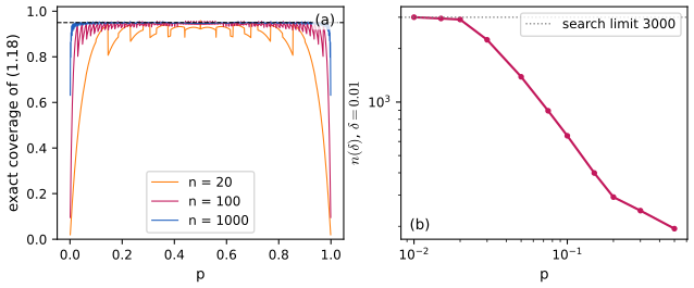
fig_1_s2. Download: PDF · SVGSee also (companion course): the exact coverage of the Wald interval and why it oscillates, and what Hoeffding's interval costs.
Example 1.20 (parametric models) p. 7
For a scalar parametric model with mle \(\hth\) and \(\hse=(I_n(\hth))^{-1/2}\), \(\hth\pm z_{\alpha/2}\hse\) is a pointwise asymptotic interval. For \(\tau=g(\theta)\), the mle is \(\widehat\tau_n=g(\hth)\) and the delta method gives \(\hse(\widehat\tau_n)=\hse(\hth)\,|g'(\hth)|\) and the interval
\[ \widehat\tau_n\pm z_{\alpha/2}\,\hse(\hth)\,|g'(\hth)|. \]Filling the gap 1.10: why the delta-method interval works, and why it is typically only pointwise p. 7
Proof
Assume the conditions of Filling the gap 1.6, that \(g\) is continuously differentiable near \(\theta\) and \(g'(\theta)\ne0\). By Result 1.6 and the delta method, \(\sqrt n(\widehat\tau_n-\tau)\wto\N(0,g'(\theta)^2/I(\theta))\). Also \(\sqrt n\,\hse(\hth)\,|g'(\hth)|=|g'(\hth)|/\sqrt{I(\hth)}\toP|g'(\theta)|/\sqrt{I(\theta)}\) by consistency and continuous mapping. By Slutsky the ratio \((\widehat\tau_n-\tau)/\hse(\widehat\tau_n)\wto\N(0,1)\), and the coverage tends to \(1-\alpha\) at each \(\theta\). ∎
Only pointwise. Every step is a limit at a fixed \(\theta\), and the speed depends on \(\theta\) through the remainder terms. Unless those bounds hold uniformly (for example, \(\Theta\) compact and the derivatives bounded uniformly), the coverage need not converge uniformly; the Bernoulli model, where \(I(p)=1/(p(1-p))\) blows up at the boundary, is the example of Filling the gap 1.9. If \(g'(\theta)=0\) the interval has length \(o_P(n^{-1/2})\) at that \(\theta\) and its coverage need not tend to \(1-\alpha\) there.
The order of preference is: a finite-sample set if one exists, otherwise a uniform asymptotic set, and only as a last resort a pointwise asymptotic set.
1.4 Useful Inequalities
pp. 8–10 Finite-sample confidence sets and the risk bounds of later chapters rest on probability inequalities. The book collects them here for reference; the boxes prove each one.
See also (companion course): Chapter 4, probability inequalities and inequalities for expectations.
Markov's and Chebyshev's inequalities p. 8, (1.21)–(1.22)
If \(X\ge0\) and \(\E X\) exists, then for \(t>0\)
\[ \P(X>t)\le\frac{\E(X)}{t}. \tag{1.21} \]If \(\mu=\E X\) and \(\sigma^2=\V(X)\), then
\[ \P(|X-\mu|\ge t)\le\frac{\sigma^2}{t^2}. \tag{1.22} \]Proof
Since \(X\ge t\,\I(X>t)\), taking expectations gives \(\E X\ge t\,\P(X>t)\). For Chebyshev apply the same inequality, \(\E Y\ge t^2\P(Y\ge t^2)\), to \(Y=(X-\mu)^2\) (with \(\ge\) in place of \(>\), by \(Y\ge t^2\I(Y\ge t^2)\)), and note \(\{|X-\mu|\ge t\}=\{Y\ge t^2\}\). Both are attained by two-point distributions; see the companion course, Filling the gap 4.1 and 4.3. ∎
Hoeffding's inequality p. 8, (1.23)–(1.24)
Let \(Y_1,\dots,Y_n\) be independent with \(\E(Y_i)=0\) and \(a_i\le Y_i\le b_i\). Then for any \(\epsilon>0\) and any \(t>0\)
\[ \P\Big(\sum_{i=1}^nY_i\ge\epsilon\Big)\le e^{-t\epsilon}\prod_{i=1}^ne^{t^2(b_i-a_i)^2/8}. \tag{1.23} \]For \(X_1,\dots,X_n\sim\Bern(p)\) and any \(\epsilon>0\),
\[ \P\big(|\Xb-p|>\epsilon\big)\le2e^{-2n\epsilon^2}. \tag{1.24} \]Filling the gap 1.11: Hoeffding's lemma, the inequality, and the best \(t\) p. 8
Proof
Lemma (Hoeffding). If \(\E Y=0\) and \(a\le Y\le b\), then \(\E e^{tY}\le e^{t^2(b-a)^2/8}\) for all real \(t\).
Proof of the lemma. If \(a=b\) then \(Y=0\). Otherwise \(a\le0\le b\). By convexity of \(y\mapsto e^{ty}\), for \(y\in[a,b]\)
\[ e^{ty}\le\frac{b-y}{b-a}e^{ta}+\frac{y-a}{b-a}e^{tb}. \]Take expectations and use \(\E Y=0\): \(\E e^{tY}\le\frac{b}{b-a}e^{ta}-\frac{a}{b-a}e^{tb}\). Put \(\gamma=-a/(b-a)\in[0,1]\) and \(u=t(b-a)\); the right side is \(e^{G(u)}\) with \(G(u)=-\gamma u+\log(1-\gamma+\gamma e^u)\). Then \(G(0)=0\), \(G'(u)=-\gamma+\rho(u)\) with \(\rho(u)=\gamma e^u/(1-\gamma+\gamma e^u)\), so \(G'(0)=0\), and \(G''(u)=\rho(u)(1-\rho(u))\le1/4\). By Taylor's theorem with the Lagrange remainder, \(G(u)\le u^2/8=t^2(b-a)^2/8\). \(\square\)
(1.23). For \(t>0\), \(\I(\sum Y_i\ge\epsilon)\le e^{t(\sum Y_i-\epsilon)}\). Take expectations, use independence to factor \(\E e^{t\sum Y_i}=\prod\E e^{tY_i}\), and apply the lemma to each factor.
The best \(t\). The exponent \(-t\epsilon+t^2S/8\), with \(S=\sum(b_i-a_i)^2\), is smallest at \(t=4\epsilon/S\), which gives the usable form
\[ \P\Big(\sum_{i=1}^nY_i\ge\epsilon\Big)\le\exp\Big(-\frac{2\epsilon^2}{\sum_i(b_i-a_i)^2}\Big). \](1.24). Put \(Y_i=X_i-p\in[-p,1-p]\), an interval of length 1. With \(n\epsilon\) in place of \(\epsilon\), \(\P(\Xb-p\ge\epsilon)\le e^{-2n^2\epsilon^2/n}=e^{-2n\epsilon^2}\). Applying this to \(-Y_i\) bounds the lower tail by the same number, and a union bound gives (1.24), even with \(\ge\) in place of \(>\). ∎
Hoeffding's bound uses only the range. Its exponent \(2\epsilon^2\) matches the CLT exponent \(\epsilon^2/(2\sigma^2)\) only when \(\sigma^2\) takes its largest possible value \(1/4\); for small variances Bernstein's inequality is much sharper (Filling the gap 1.14). The companion course proves the lemma in the same way, Result 4.12.
Mill's inequality p. 8, (1.25)–(1.27)
If \(Z\sim\N(0,1)\) and \(t>0\),
\[ \P(|Z|>t)\le\frac{2\phi(t)}{t}, \tag{1.25} \] \[ \Big(\frac1t-\frac1{t^3}\Big)\phi(t)\lt \P(Z>t)\lt \frac1t\,\phi(t), \tag{1.26} \] \[ \P(Z>t)\lt \tfrac12e^{-t^2/2}. \tag{1.27} \]Filling the gap 1.12: proofs of Mill's inequalities p. 8
Proof
All three use \(\phi'(z)=-z\phi(z)\).
Upper bound in (1.26). On \((t,\infty)\), \(z/t>1\), so \(\P(Z>t)=\int_t^\infty\phi(z)\,\d z\lt \int_t^\infty\frac zt\phi(z)\,\d z=\frac{\phi(t)}t\). Then (1.25) follows by symmetry, \(\P(|Z|>t)=2\P(Z>t)\).
Lower bound in (1.26). Differentiation gives \(\big(\phi(z)/z\big)'=-\phi(z)\big(1+z^{-2}\big)\) and \(\big(\phi(z)/z^3\big)'=-\phi(z)\big(z^{-2}+3z^{-4}\big)\). Integrating from \(t\) to \(\infty\):
\[ \frac{\phi(t)}t=\P(Z>t)+\int_t^\infty\frac{\phi(z)}{z^2}\,\d z,\qquad \int_t^\infty\frac{\phi(z)}{z^2}\,\d z=\frac{\phi(t)}{t^3}-3\int_t^\infty\frac{\phi(z)}{z^4}\,\d z\lt \frac{\phi(t)}{t^3}. \]Hence \(\P(Z>t)>\phi(t)/t-\phi(t)/t^3\). (For \(t\le1\) the lower bound is not positive and says nothing.) Continuing the integration by parts gives the asymptotic series \(\P(Z>t)\sim\frac{\phi(t)}t\big(1-t^{-2}+3t^{-4}-\dots\big)\), whose partial sums alternate between upper and lower bounds.
(1.27). Substitute \(z=t+u\): \(\phi(t+u)=\phi(t)e^{-tu}e^{-u^2/2}\), so
\[ \P(Z>t)=\phi(t)\int_0^\infty e^{-tu-u^2/2}\,\d u\lt \phi(t)\int_0^\infty e^{-u^2/2}\,\d u=\phi(t)\sqrt{\pi/2}=\tfrac12e^{-t^2/2}. \]The Chernoff bound \(\P(Z>t)\le\inf_se^{-st}\E e^{sZ}=e^{-t^2/2}\) is twice as large; (1.26) is sharper still for \(t>\sqrt{2/\pi}\approx0.8\), where \(\phi(t)/t\lt \frac12e^{-t^2/2}\). ∎
Mill's inequality is the tool for Normal maxima: for \(Z_1,\dots,Z_n\) iid \(\N(0,1)\), a union bound and (1.26) give \(\P(\max_i|Z_i|>\sqrt{2\log n})\le2n\phi(\sqrt{2\log n})/\sqrt{2\log n}=1/\sqrt{\pi\log n}\to0\). This is the "universal threshold" of wavelet thresholding in Chapter 9.
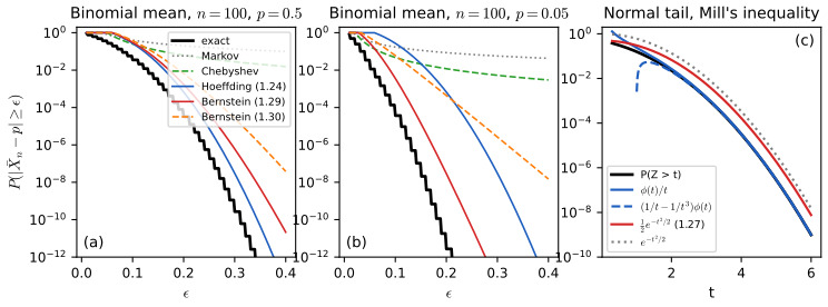
fig_1_s3. Download: PDF · SVGThe Berry-Esseen bound p. 9, (1.28)
Let \(X_1,\dots,X_n\) be iid with mean \(\mu\), variance \(\sigma^2>0\) and \(\E|X_1|^3\lt \infty\), and \(Z_n=\sqrt n(\Xb-\mu)/\sigma\). Then
\[ \sup_z\big|\P(Z_n\le z)-\Phi(z)\big|\le\frac{33}{4}\,\frac{\E|X_1-\mu|^3}{\sqrt n\,\sigma^3}. \tag{1.28} \]Filling the gap 1.13: the constant, the rate, and how the bound is proved p. 9
The constant. (1.28) is true with \(33/4\) (an early published value), but much smaller constants are known: the inequality holds with \(C=0.4748\) in place of \(33/4\) (Shevtsova 2011), and no constant below \(C_0=(\sqrt{10}+3)/(6\sqrt{2\pi})\approx0.4097\) can work (Esseen 1956). So the book's bound is valid but about 17 times too generous. Figure 1.S4 compares both constants with the exact distance.
The rate \(n^{-1/2}\) is optimal (proof), and the structure of the proof of (1.28)
The rate cannot be improved. Take \(X_i\sim\Bern(1/2)\), \(n=2m\) even. Then \(Z_n\) has an atom at \(0\) of mass \(\binom{2m}m2^{-2m}\ge1/(2\sqrt m)\) (a standard bound, e.g. by Wallis' product). Because \(\Phi\) is continuous, \(|\P(Z_n\le z)-\Phi(z)|\) is at least half the jump either just left of 0 or at 0: the distance is at least \(1/(4\sqrt m)=1/(2\sqrt{2n})\). So no bound of smaller order than \(n^{-1/2}\) can hold for all distributions with three moments.
How (1.28) is proved. The classical proof has two steps. (i) Esseen's smoothing inequality: for a cdf \(G\) with \(|G'|\le m\) and any cdf \(H\) with characteristic functions \(\gamma,\eta\), and any \(T>0\),
\[ \sup_z|H(z)-G(z)|\le\frac1\pi\int_{-T}^T\Big|\frac{\eta(s)-\gamma(s)}{s}\Big|\,\d s+\frac{24m}{\pi T}. \]It comes from convolving both cdfs with a smooth kernel whose Fourier transform vanishes outside \([-T,T]\) and controlling what the smoothing loses. (ii) A Taylor expansion of the characteristic function of \((X_1-\mu)/\sigma\) to third order, with \(\rho=\E|X_1-\mu|^3/\sigma^3\), shows that for \(|s|\le\sqrt n/(4\rho)\),
\[ \big|\eta_n(s)-e^{-s^2/2}\big|\le\frac{16\rho}{\sqrt n}|s|^3e^{-s^2/3}, \]where \(\eta_n\) is the characteristic function of \(Z_n\). Putting (ii) into (i) with \(T=\sqrt n/(4\rho)\) gives a bound \(C\rho/\sqrt n\) with an explicit \(C\). Feller (1971, Section XVI.5) carries this out in full; the companion course discusses the constant and the shape of the error in Filling the gap 5.9. The sharper constants above require a much finer analysis. \(\square\)
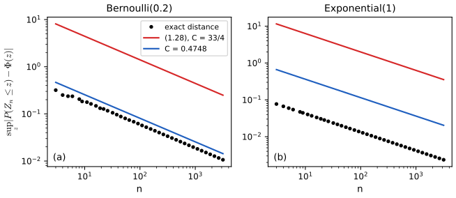
fig_1_s4. Download: PDF · SVGSee also (companion course): the Berry-Esseen demo.
Bernstein's inequalities p. 9, (1.29)–(1.30)
Let \(X_1,\dots,X_n\) be independent with mean zero and \(-M\le X_i\le M\). Then for \(t>0\)
\[ \P\Big(\Big|\sum_{i=1}^nX_i\Big|>t\Big)\le2\exp\Big\{-\frac12\,\frac{t^2}{v+Mt/3}\Big\},\qquad v\ge\sum_{i=1}^n\V(X_i). \tag{1.29} \]Moment version. If instead the \(X_i\) are independent with mean zero and \(\E|X_i|^m\le m!\,M^{m-2}v_i/2\) for all \(m\ge2\), then with \(v=\sum_iv_i\)
\[ \P\Big(\Big|\sum_{i=1}^nX_i\Big|>t\Big)\le2\exp\Big\{-\frac12\,\frac{t^2}{v+Mt}\Big\}. \tag{1.30} \]Filling the gap 1.14: proofs of Bernstein's inequalities, and when they beat Hoeffding p. 9
Proof
Step 1: the moment generating function under the moment condition. For \(0\le\lambda\lt 1/M\), expanding the exponential (the interchange of sum and expectation is justified by \(\E e^{\lambda|X_i|}\lt \infty\), which the moment condition implies),
\[ \E e^{\lambda X_i}=1+\lambda\E X_i+\sum_{m\ge2}\frac{\lambda^m\E X_i^m}{m!}\le1+\frac{\lambda^2v_i}2\sum_{m\ge2}(\lambda M)^{m-2}=1+\frac{\lambda^2v_i}{2(1-\lambda M)}\le\exp\Big\{\frac{\lambda^2v_i}{2(1-\lambda M)}\Big\}. \]Step 2: Chernoff. By independence, \(\P(\sum_iX_i>t)\le e^{-\lambda t}\prod_i\E e^{\lambda X_i}\le\exp\{-\lambda t+\lambda^2v/(2(1-\lambda M))\}\). Choose \(\lambda=t/(v+Mt)\), which is below \(1/M\). Then \(1-\lambda M=v/(v+Mt)\), so
\[ -\lambda t+\frac{\lambda^2v}{2(1-\lambda M)}=-\frac{t^2}{v+Mt}+\frac{t^2}{2(v+Mt)}=-\frac{t^2}{2(v+Mt)}. \]The variables \(-X_i\) satisfy the same condition, which bounds the lower tail; adding the two gives (1.30).
Bounded variables, (1.29). If \(|X_i|\le M\) then \(\E|X_i|^m\le M^{m-2}\E X_i^2=M^{m-2}\sigma_i^2\). Since \(m!\ge2\cdot3^{m-2}\) for \(m\ge2\) (equality at \(m=2,3\); each further factor is at least 4), we get \(\E|X_i|^m\le m!\,(M/3)^{m-2}\sigma_i^2/2\): the moment condition holds with \(M/3\) in place of \(M\) and \(v_i=\sigma_i^2\). So (1.30) with \(M/3\) gives (1.29) with \(v=\sum_i\sigma_i^2\); and the bound only grows if \(v\) is replaced by anything larger. ∎
Comparison with Hoeffding. For the mean of \(n\) variables with \(|X_i-\mu|\le M\) and variance \(\sigma^2\), (1.29) with \(t=n\epsilon\) gives the exponent \(-n\epsilon^2/(2\sigma^2+2M\epsilon/3)\). For small \(\epsilon\) this is about \(-n\epsilon^2/(2\sigma^2)\), the CLT exponent; Hoeffding gives \(-n\epsilon^2/(2M^2)\), using the range \(2M\). So Bernstein wins when \(\sigma^2\ll M^2\) and \(\epsilon\) is not too large. With no information on the variance (\(\sigma^2\le M^2\) is all one knows) Bernstein is never better than Hoeffding: Figure 1.S5(b) and Exercise 1.5(c).
The Cauchy-Schwarz and Jensen inequalities pp. 9–10, (1.31)–(1.33)
If \(X\) and \(Y\) have finite variances,
\[ \E|XY|\le\sqrt{\E(X^2)\,\E(Y^2)}. \tag{1.31} \]A function \(g\) is convex if \(g(\alpha x+(1-\alpha)y)\le\alpha g(x)+(1-\alpha)g(y)\) for all \(x,y\) and \(\alpha\in[0,1]\), and concave if \(-g\) is convex. If \(g\) is convex and \(\E|X|\), \(\E|g(X)|\) are finite, then
\[ \E g(X)\ge g(\E X), \tag{1.32} \]and if \(g\) is concave,
\[ \E g(X)\le g(\E X). \tag{1.33} \]Filling the gap 1.15: Cauchy-Schwarz, the tangent-line property and Jensen pp. 9–10
Proof
Cauchy-Schwarz. Put \(U=|X|\), \(W=|Y|\). If \(\E W^2=0\) then \(W=0\) almost surely and both sides are 0. Otherwise, for every real \(s\), \(0\le\E(U-sW)^2=\E U^2-2s\E(UW)+s^2\E W^2\). A quadratic in \(s\) that is never negative has a non-positive discriminant: \((\E UW)^2\le\E U^2\,\E W^2\).
\(g''\ge0\) implies convexity. Let \(x\lt y\), \(z=\alpha x+(1-\alpha)y\). By the mean value theorem there are \(\xi_1\in(x,z)\), \(\xi_2\in(z,y)\) with \(g(z)-g(x)=g'(\xi_1)(z-x)\) and \(g(y)-g(z)=g'(\xi_2)(y-z)\). As \(g'\) is nondecreasing, \(g'(\xi_1)\le g'(\xi_2)\); multiply the first identity by \(\alpha\), the second by \(1-\alpha\), use \(\alpha(z-x)=(1-\alpha)(y-z)\), and subtract to get \(\alpha g(x)+(1-\alpha)g(y)-g(z)\ge0\).
The tangent line ("it can be shown"). Let \(g\) be convex on \(\R\) and fix \(x_0\). Convexity is equivalent to the slopes \(\sigma(u,v)=(g(v)-g(u))/(v-u)\) being nondecreasing in each argument (apply the definition to three points \(u\lt w\lt v\)). Hence the left derivative \(g'_-(x_0)=\lim_{u\uparrow x_0}\sigma(u,x_0)\) and the right derivative \(g'_+(x_0)=\lim_{v\downarrow x_0}\sigma(x_0,v)\) exist, are finite and satisfy \(\sigma(u,x_0)\le g'_-(x_0)\le g'_+(x_0)\le\sigma(x_0,v)\) for \(u\lt x_0\lt v\). Take any \(c\in[g'_-(x_0),g'_+(x_0)]\). For \(v>x_0\), \(g(v)-g(x_0)\ge c(v-x_0)\); for \(u\lt x_0\), \(g(x_0)-g(u)\le c(x_0-u)\). Together: \(g(x)\ge g(x_0)+c(x-x_0)\) for all \(x\). (When \(g\) is differentiable, \(c=g'(x_0)\) and the line is the tangent.)
Jensen. Take \(x_0=\E X\) and integrate the line: \(\E g(X)\ge g(\E X)+c(\E X-\E X)=g(\E X)\). For concave \(g\) apply this to \(-g\). ∎
Jensen gives, for example, \(\E\log X\le\log\E X\) and \(\big(\E|X|\big)^2\le\E X^2\), and Gibbs' inequality \(\mathrm{KL}\ge0\) (companion course, Result 4.10).
See also (companion course): the Cauchy-Schwarz inequality, Jensen's inequality and the Jensen demo.
Two small points in Section 1.4 pp. 9–10
(i) The inequality (1.31) is printed under the name "Cauchy-Schwartz"; the second name is Schwarz (Hermann Amandus Schwarz). (ii) Jensen's inequality, as printed, has no integrability condition; it needs \(\E|X|\lt \infty\) and \(\E g(X)\) to be defined (possibly \(+\infty\) for convex \(g\)), as stated above. Neither affects any result.
1.5 Bibliographic Remarks
p. 10 For probability inequalities and their use in statistics and pattern recognition the book points to Devroye, Györfi and Lugosi (1996) and van der Vaart and Wellner (1996); for a review of probability and mathematical statistics, to Casella and Berger (2002), van der Vaart (1998) and Wasserman (2004), the last being the text of the companion course Probability and Statistical Inference. For the proportion interval of Example 1.17, Brown, Cai and DasGupta (2001) is the standard reference; Bahadur and Savage (1956) is the classical source for the impossibility result behind Exercise 1.5(b).
1.6 Exercises
All five exercises of Chapter 1 (Wasserman, 2006, pp. 10–11), restated in my own words, with complete solutions (hidden). Computational answers come from ch01_introduction.py.
Exercise 1.1. In Example 1.17, show that the Wald interval (1.18) is a pointwise asymptotic confidence interval and that Hoeffding's interval (1.19) is a uniform one.
Solution
Both parts are proved in Filling the gap 1.9. In brief: for each fixed \(p\in(0,1)\) the CLT, the weak law and Slutsky give \(\sqrt n(\hp-p)/\sqrt{\hp(1-\hp)}\wto\N(0,1)\), so the Wald coverage tends to \(1-\alpha\); at \(p\in\{0,1\}\) it is 1. Hoeffding's inequality (1.24) with \(\epsilon_n=\sqrt{\log(2/\alpha)/(2n)}\) gives \(\P_p(|\hp-p|>\epsilon_n)\le\alpha\) for every \(p\) and every \(n\). This is the finite-sample property (1.12), which is stronger than what the exercise asks: by Filling the gap 1.8 it implies (1.13). The Wald interval is not uniform: its coverage at \(p=1/n^2\) is at most \(1/n\).
Exercise 1.2 (computer experiment). For \(p=0.2\) and \(\alpha=0.05\), compare the coverage and length of (1.18) and (1.19) for several \(n\). How large must \(n\) be for the Wald interval to have accurate coverage, and how do the lengths compare at that \(n\)?
Solution
Rather than simulate, sum over the Binomial(\(n,0.2\)) law: the coverage is \(\sum_k\binom nk0.2^k0.8^{n-k}\I(p\in C_n(k))\) exactly, and similarly the expected length (functions
coverage_exactandexpected_length).\(n\) Wald coverage Hoeffding coverage Wald mean length Hoeffding length 10 0.886 0.999 0.400 0.859 20 0.921 0.999 0.326 0.607 50 0.938 0.999 0.218 0.384 100 0.933 0.999 0.156 0.272 200 0.941 0.999 0.110 0.192 500 0.949 0.999 0.070 0.122 1000 0.947 0.999 0.050 0.086 How large? Because the coverage oscillates in \(n\) (Figure 1.S1(a)), "accurate" must mean "stays accurate". Taking it as "coverage at least 0.94 for every larger \(n\)" (\(\delta=0.01\)), the answer is \(n=292\) (checked up to \(n=3000\)); below that the coverage dips to 0.82 at \(n=15\) and to about 0.93 near \(n=100\).
Lengths. At \(n=292\) Hoeffding's interval has length 0.159 and the Wald interval mean length 0.092: a ratio of 1.74. The ratio tends to \(\sqrt{\log(2/\alpha)/2}\,/\,\big(z_{\alpha/2}\sqrt{p(1-p)}\big)=1.358/0.784=1.73\), so for \(p=0.2\) the guarantee costs about 73% more length, at every large \(n\). Meanwhile Hoeffding's coverage is 0.999: it is conservative, because it must protect against \(p=1/2\) and uses only the range.
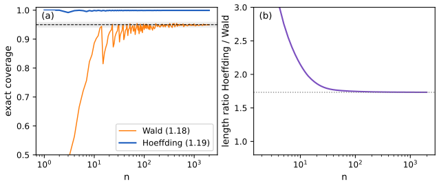
Figure 1.S1 (supplementary). Exercise 1.2: \(p=0.2\), \(\alpha=0.05\). (a) Exact coverage of (1.18) and (1.19); the grey band is \(0.95\pm0.01\). (b) Length of (1.19) divided by the expected length of (1.18); the dotted line is the limit 1.73. Not a figure of the book. Code: ch01_introduction.py, fig_1_s1. Download: PDF · SVGExercise 1.3. For \(X_1,\dots,X_n\sim\N(\mu,1)\), is \(C_n=\Xb\pm z_{\alpha/2}/\sqrt n\) a finite-sample, uniform asymptotic or pointwise asymptotic confidence set for \(\mu\)?
Solution
Finite-sample (hence also the other two). \(\Xb\sim\N(\mu,1/n)\) exactly, so \(\sqrt n(\Xb-\mu)\sim\N(0,1)\) for every \(\mu\) and \(n\), and \(\P_\mu(\mu\in C_n)=\P(|Z|\le z_{\alpha/2})=1-\alpha\) exactly. The infimum over \(\mu\in\R\) is \(1-\alpha\) for every \(n\).
Exercise 1.4. For \(X_1,\dots,X_n\sim\N(\mu,\sigma^2)\), with \(S_n^2=\sum_i(X_i-\Xb)^2/(n-1)\), is \(C_n=\Xb\pm z_{\alpha/2}S_n/\sqrt n\) finite-sample, uniform asymptotic or pointwise asymptotic for \(\mu\)?
Solution
Uniform asymptotic, but not finite-sample. The statistic \(T=\sqrt n(\Xb-\mu)/S_n\) has Student's \(t\) distribution with \(n-1\) degrees of freedom, whatever \(\mu\) and \(\sigma\) (independence of \(\Xb\) and \(S_n\) for Normal data). So the coverage \(\P(|t_{n-1}|\le z_{\alpha/2})\) does not depend on \((\mu,\sigma)\): the infimum over the model equals the coverage itself. The \(t\) law has heavier tails than the Normal, so the coverage is below \(1-\alpha\) for every \(n\): 0.878 at \(n=5\) and 0.944 at \(n=50\) for \(\alpha=0.05\). As \(n\to\infty\), \(t_{n-1}\wto\N(0,1)\), so the coverage, which is also the infimum, tends to \(1-\alpha\). (Replacing \(z_{\alpha/2}\) by the \(t_{n-1}\) quantile gives a finite-sample interval with coverage exactly \(1-\alpha\).)
Exercise 1.5. Let \(X_1,\dots,X_n\sim F\) with mean \(\mu\), and \(C_n=\Xb\pm z_{\alpha/2}\hse\) with \(\hse^2=S_n^2/n\), \(S_n^2=n^{-1}\sum_i(X_i-\Xb)^2\). (a) Show that \(C_n\) is a pointwise asymptotic \(1-\alpha\) interval. (b) Show that it is not uniform. (Hint: with \(a_n\to\infty\), \(\epsilon_n\to0\), let \(G_n=(1-\epsilon_n)F+\epsilon_n\delta_{a_n}\).) (c) If \(\P(|X_i|\le B)=1\) for a known \(B\), use Bernstein's inequality (1.29) to build a finite-sample interval.
Solution
(a) Suppose \(0\lt \sigma^2=\V_F(X)\lt \infty\). By the CLT \(\sqrt n(\Xb-\mu)/\sigma\wto\N(0,1)\); by the weak law applied to \(X_i\) and \(X_i^2\), \(S_n^2=n^{-1}\sum X_i^2-\Xb^2\toP\sigma^2\); by Slutsky \(\sqrt n(\Xb-\mu)/S_n\wto\N(0,1)\), and the coverage tends to \(1-\alpha\). (If \(\sigma^2=0\), \(X_i=\mu\) and the coverage is 1.)
A correction: a finite mean is not enough. The exercise says "assuming that the mean exists", but the argument needs a finite variance (more precisely, \(F\) must lie in the domain of attraction of the Normal law, which allows some infinite-variance laws with slowly growing truncated second moment: Giné, Götze and Mason 1997). For laws in the domain of attraction of a stable law of index \(1\lt \gamma\lt 2\), which have a mean but no variance, the self-normalised mean \(\sqrt n(\Xb-\mu)/S_n\) converges to a non-Normal limit (Logan, Mallows, Rice and Shepp 1973), and the coverage does not tend to 0.95. Numerically, for the Pareto law with \(\P(X>x)=x^{-1.5}\), \(x\ge1\) (mean 3), the coverage of the 95% interval is 0.70, 0.75 and 0.79 at \(n=10^2,10^3,10^4\) (Monte Carlo, 20 000, 10 000 and 3000 samples).
(b) Let \(F\) have a finite variance and \(G_n=(1-\epsilon_n)F+\epsilon_n\delta_{a_n}\), with \(n\epsilon_n\to0\) and \(\epsilon_na_n\to\infty\); for instance \(\epsilon_n=n^{-3/2}\), \(a_n=n^2\). Each \(G_n\) has finite variance, so it belongs to any model that contains all finite-variance laws. Its mean is \(\mu_n=(1-\epsilon_n)\mu_F+\epsilon_na_n\to\infty\). Let \(E_n\) be the event that no observation equals \(a_n\) (more precisely, that every observation came from the \(F\) component); \(\P(E_n)=(1-\epsilon_n)^n\ge1-n\epsilon_n\to1\). On \(E_n\) the sample is an iid sample from \(F\), so \(\Xb\) and \(S_n\) have their \(F\)-distributions and the interval is \(\Xb\pm z_{\alpha/2}S_n/\sqrt n\), which lies in a bounded region with high probability (\(\Xb\toP\mu_F\), \(S_n\toP\sigma_F\)) and so excludes \(\mu_n\to\infty\). Precisely: for any \(K\),
\[ \P_{G_n}(\mu_n\in C_n)\le\P(E_n^c)+\P_F\big(\Xb+z_{\alpha/2}S_n/\sqrt n\ge\mu_n\big)\to0. \]Hence \(\inf_{G}\P_G(\mu(G)\in C_n)\to0\), and \(C_n\) is not uniform. No other interval does better: by a theorem of Bahadur and Savage (1956), any interval whose coverage of the mean is at least \(1-\alpha\) for every distribution in such a class must be unbounded with probability at least \(1-\alpha\) under every distribution in the class. Figure 1.S5(a) computes the coverage exactly for \(F=\Bern(0.3)\): 0.95 for \(F\), but 0.28 at \(n=10\) and 0.049 at \(n=398\) along \(G_n\).
(c) Put \(Y_i=X_i-\mu\). Then \(|Y_i|\le2B\) and \(\V(Y_i)\le\E X_i^2\le B^2\), so (1.29) applies with \(M=2B\) and \(v=nB^2\). Setting \(L=\log(2/\alpha)\) and solving \(t^2=2L(v+Mt/3)\) for the positive root,
\[ t_n=\frac{2BL}{3}+\sqrt{\Big(\frac{2BL}{3}\Big)^2+2nB^2L},\qquad C_n=\Xb\pm\frac{t_n}{n}, \]and \(\P(\mu\notin C_n)=\P(|\sum Y_i|>t_n)\le\alpha\) for every \(F\) with support in \([-B,B]\) and every \(n\). Its half-width is \(B\sqrt{2L/n}+O(1/n)\). Hoeffding's inequality with range \(2B\) gives the half-width \(B\sqrt{2L/n}\) exactly, which is never larger: without information on the variance Bernstein brings nothing. If a bound \(\sigma^2\le s^2\) with \(s\ll B\) is known, replacing \(v=nB^2\) by \(ns^2\) gives a half-width close to \(s\sqrt{2L/n}\), much shorter (Figure 1.S5(b)). The same bounded-support assumption is what rescues uniformity in (b): \(G_n\) has support up to \(a_n\to\infty\), which the bound \(B\) excludes.
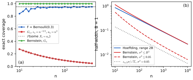
fig_1_s5. Download: PDF · SVGDemonstrations for this chapter
Each demonstration runs in the browser and links back to these notes. The ▶ Demo boxes above open them already set to the case under discussion.
| Demonstration | What you can see | Sections and results |
|---|---|---|
| Pointwise and uniform coverage | The exact coverage of the Wald and Hoeffding intervals against \(p\) and against \(n\), the worst case over \(p\), and \(n(\delta)\). Presets: 1 \(n=20\); 2 \(n=1000\); 3 Exercise 1.2; 4 \(p=0.01\); 5 \(\alpha=0.1\). | Section 1.3; 1.8, 1.9; Exercises 1.1, 1.2 |
| Tail inequalities against exact tails | Markov, Chebyshev, Hoeffding and both Bernstein bounds against the exact Binomial tail; Mill's bounds against the Normal tail. Presets: 1 fair coin; 2 rare event; 3 small deviations; 4 \(n=1000\); 5 Mill at \(t=3\). | Section 1.4; 1.11, 1.12, 1.14 |
| The interval for a mean under contamination | The exact coverage of \(\Xb\pm z\,\hse\), Hoeffding's and Bernstein's intervals for a contaminated Bernoulli population, and along the sequence \(G_n\). Presets: 1 no contamination; 2 1% at 50; 3 the sequence \(G_n\); 4 larger \(n\); 5 Bernstein with the true variance. | Section 1.3; Exercise 1.5; 1.14 |
Related demonstrations in the companion course Probability and Statistical Inference: Hoeffding's interval for a proportion, coverage of confidence intervals, the Berry-Esseen bound, the delta method, modes of convergence and Jensen's inequality. The Python code that produces every figure of this page is code/ch01_introduction.py; see the code index.
References
- Wasserman, L. (2006). All of Nonparametric Statistics. Springer, New York. Chapter 1, pp. 1–11. www.stat.cmu.edu/~larry/all-of-nonpar.
- Bahadur, R. R. and Savage, L. J. (1956). The nonexistence of certain statistical procedures in nonparametric problems. The Annals of Mathematical Statistics, 27(4), 1115–1122.
- Berry, A. C. (1941). The accuracy of the Gaussian approximation to the sum of independent variates. Transactions of the American Mathematical Society, 49(1), 122–136.
- Brown, L. D., Cai, T. T. and DasGupta, A. (2001). Interval estimation for a binomial proportion. Statistical Science, 16(2), 101–133.
- Casella, G. and Berger, R. L. (2002). Statistical Inference, 2nd edition. Duxbury, Pacific Grove.
- Devroye, L., Györfi, L. and Lugosi, G. (1996). A Probabilistic Theory of Pattern Recognition. Springer, New York.
- Esseen, C.-G. (1942). On the Liapounoff limit of error in the theory of probability. Arkiv för Matematik, Astronomi och Fysik, 28A(9), 1–19.
- Esseen, C.-G. (1956). A moment inequality with an application to the central limit theorem. Skandinavisk Aktuarietidskrift, 39, 160–170.
- Feller, W. (1971). An Introduction to Probability Theory and Its Applications, Volume II, 2nd edition. Wiley, New York.
- Giné, E., Götze, F. and Mason, D. M. (1997). When is the Student \(t\)-statistic asymptotically standard normal? The Annals of Probability, 25(3), 1514–1531.
- Hoeffding, W. (1963). Probability inequalities for sums of bounded random variables. Journal of the American Statistical Association, 58(301), 13–30.
- Logan, B. F., Mallows, C. L., Rice, S. O. and Shepp, L. A. (1973). Limit distributions of self-normalized sums. The Annals of Probability, 1(5), 788–809.
- Shevtsova, I. G. (2011). On the absolute constants in the Berry-Esseen type inequalities for identically distributed summands. Preprint, arXiv:1111.6554.
- van der Vaart, A. W. (1998). Asymptotic Statistics. Cambridge University Press, Cambridge.
- van der Vaart, A. W. and Wellner, J. A. (1996). Weak Convergence and Empirical Processes. Springer, New York.
- Wasserman, L. (2004). All of Statistics: A Concise Course in Statistical Inference. Springer, New York.
The numerical statements in the text (the exact coverages and lengths of Exercise 1.2, the sample sizes \(n(\delta)\), the tail probabilities and bounds of Section 1.4, the Berry-Esseen distances, the Student-\(t\) coverages of Exercise 1.4, and the contamination coverages of Exercise 1.5) were confirmed numerically.