Smoothing: General Concepts
Every curve estimator in the rest of the course, whether a histogram, a kernel density estimate, a local regression or a wavelet fit, has a knob that sets how much it averages. This chapter introduces the two problems (density estimation and regression), shows on real data what happens when the knob is set too low or too high, and explains why: the risk splits into a squared bias that grows with smoothing and a variance that shrinks with it. It then fixes the vocabulary used later (kernels, loss functions, integrated risk, confidence balls and bands) and ends with the statistical curse of dimensionality: the rate \(n^{-4/(4+d)}\) that makes local smoothing hopeless in high dimensions.
Ch. 1 Introduction Ch. 2 The cdf and functionals Ch. 3 Bootstrap and jackknife Ch. 4 Smoothing Ch. 5 Regression Ch. 6 Density estimation Ch. 7 Normal means and minimax Ch. 8 Orthogonal functions Ch. 9 Wavelets Ch. 10 Other topics
How to read these notes
They follow the book. Sections carry the book's numbers (4.1, 4.2, ...) and every displayed equation that appears in the book carries the book's own equation number, e.g. \((4.10)\), so you can read these notes next to the book. Equations without a number are steps that the book skips. The examples before Section 4.1 are grouped under an unnumbered heading.
Filling the gaps. Wherever the book states a result without proof, leaves it to an exercise or quotes it from the literature, a Filling the gap box or a proof gives the full argument. Proofs and derivations start hidden: open one with its bar, or use the button below.
Figures and demonstrations. Every figure of the chapter that is computed from data or a model is reproduced from scratch by the Python code, including Figure 4.9, which the book draws as a schematic and which is computed here exactly. The ▶ Demo boxes open an interactive demonstration already set to the case being discussed.
Main reference
L. Wasserman, All of Nonparametric Statistics, Springer (2006), Chapter 4, pages 43–60 (book website, with the data sets: www.stat.cmu.edu/~larry/all-of-nonpar). Section, equation, figure and exercise numbers below refer to this book. Further reading is listed in the references.
The explanations, derivations, figures and code are my own; equations are cited by their numbers in the book.
Companion courses
This chapter is the general introduction to smoothing; several companion courses on this site cover parts of it at an easier or a different level:
- Probability and Statistical Inference (Wasserman 2004, same author and notation), Chapter 20: the bias–variance decomposition (Section 20.1), histograms and their cross-validation score on the same galaxy data (20.2, Figure 20.3), kernel density estimation (20.3) and kernel regression (20.4); Fisher information in Section 9.7.
- Statistical Learning: Theory and Methods: local methods in high dimensions (Section 2.5), kernel smoothers and local likelihood (Sections 6.1 and 6.5), the bias–variance decomposition and cross-validation (Sections 7.3 and 7.10), additive models and backfitting (Section 9.1).
- Bayesian and Probabilistic Machine Learning: histograms, kernel density estimators and nearest neighbours (Section 2.5).
- Demonstrations of the same ideas: histogram cross-validation and kernel regression with a band (Probability and Statistical Inference), curse of dimensionality and kernel density bandwidth (Statistical Learning), bias and variance (Bayesian and Probabilistic Machine Learning).
Where a proof there is complete, these notes give the statement and a short argument and link to it. New here: the exact binomial analysis of Example 4.16 with its remainder terms and what happens at a cusp, the constants of the four kernels, the invariance of the \(L_1\) loss and the tail sensitivity of the Kullback–Leibler loss, the relation between bands and balls, a corrected sample-size formula for the curse of dimensionality, and the \(d\)-dimensional version of Example 4.16.
The chapter at a glance
- Examples 4.3–4.7 Density estimation (galaxy redshifts) and regression (CMB spectrum, LIDAR, BPD, rock permeability): each estimator has a smoothing parameter, and the picture depends on it (Figures 4.1–4.8).
- 4.1 Risk = bias\(^2\) + variance, pointwise and integrated (Result 4.10); the average risk equals the predictive risk minus \(\sigma^2\) (Result 4.14); for the counting estimator of \(f(0)\) the mse is \(Ah^4+B/(nh)\), with best \(h\propto n^{-1/5}\) and mse \(\propto n^{-4/5}\) (Result 4.16).
- 4.2 Kernels and the local average (4.23)–(4.24): the constants \(\sigma_K^2\) and \(\int K^2\) of the four standard kernels (Filling the gap 4.3).
- 4.3 \(L_1\) is invariant under changes of variable, \(L_2\) is not; Kullback–Leibler loss can be infinite because of the tails (Filling the gap 4.4).
- 4.4 Confidence balls and bands; a band gives a ball (Filling the gap 4.5).
- 4.5 Small neighbourhoods are empty in high dimensions; the sample size for a fixed accuracy grows like \(\delta^{-(4+d)/4}\) (Filling the gap 4.6).
Notation. \(X_1,\dots,X_n\sim f\) for density estimation; \(Y_i=r(x_i)+\epsilon_i\) with \(\E\epsilon_i=0\) for regression; \(\hf_n\), \(\hr_n\) estimators; \(h\) a smoothing parameter (bin width or bandwidth); \(\phi\) and \(\Phi\) the standard Normal density and cdf; \(\I(\cdot)\) an indicator.
Prerequisites. Expectation and variance, the binomial distribution, Taylor's theorem with remainder, and the basic smoothing ideas of Chapter 20 of the companion course.
Two problems, five examples
p. 43 The book studies two estimation problems.
Definition 4.1 (the two smoothing problems) p. 43, (4.1)–(4.2)
Density estimation. Observe \(X_1,\dots,X_n\) independent with common density \(f\),
\[ X_1,\dots,X_n\sim f, \tag{4.1} \]and estimate the function \(f\).
Regression. Observe pairs \((x_1,Y_1),\dots,(x_n,Y_n)\) with
\[ Y_i=r(x_i)+\epsilon_i,\qquad \E(\epsilon_i)=0, \tag{4.2} \]and estimate the regression function \(r\). With random covariates, \(r(x)=\E(Y\given X=x)\).
In both problems the target is a whole function, not a finite list of parameters, and only weak assumptions (smoothness, typically) are made about it. An estimate is obtained by smoothing: averaging the data that are close to the point of interest. How far "close" extends is the smoothing parameter.
Example 4.3: galaxy redshifts (density estimation)
pp. 43–45 The data are redshifts of galaxies along a narrow "pencil beam" from the Sloan Digital Sky Survey. Redshift measures distance, and clusters of galaxies show up as peaks of the density \(f\) of the redshifts. Keeping the 1266 galaxies with redshift below 0.2, a histogram with bins of width \(h\) estimates \(f\) by the proportion of points in each bin divided by \(h\). Many narrow bins give a spiky, noisy estimate (undersmoothing: small bias, large variance); a few wide bins blur the clusters away (oversmoothing: large bias, small variance). The lower right panel of Figure 4.1 shows an estimate of the risk as a function of the number of bins, computed from the data alone by leave-one-out cross-validation (Filling the gap 4.7).
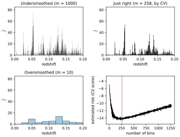
fig_4_1. Reproduces Wasserman (2006), Figure 4.1. Download: PDF · SVGFigure 4.2 of the book is a sketch of the pencil-beam geometry and Figure 4.4 is the WMAP satellite map of the sky; neither is computed from data, so neither is reproduced.
A kernel density estimator (Chapter 6) replaces the fixed bins by a smooth bump of width \(h\) centred at every observation, \(\hf_n(x)=n^{-1}\sum_i h^{-1}K((x-X_i)/h)\). Figure 4.3 shows the same trade-off. The cross-validated bandwidth is small, because the galaxy clusters are narrow and \(n\) is large enough to resolve them.
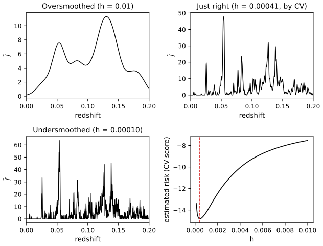
fig_4_3, kde_lscv. Reproduces Wasserman (2006), Figure 4.3. Download: PDF · SVGSee also (companion courses): histograms and kernel density estimation in Probability and Statistical Inference, with the histogram cross-validation demo.
Example 4.4: the cosmic microwave background (regression)
pp. 45–47 The temperature of the microwave background varies slightly across the sky; its power spectrum \(r(x)\), the strength of the fluctuations at multipole (frequency) \(x\), carries information about the composition of the early universe. After a long reduction the WMAP data become pairs \((x_i,Y_i)\), \(Y_i=r(x_i)+\epsilon_i\), with \(Y_i\) an estimate of the power at \(x_i\). For the first 400 multipoles the noise variance is roughly constant. Figure 4.5 shows a local linear fit (Chapter 5) with three bandwidths.
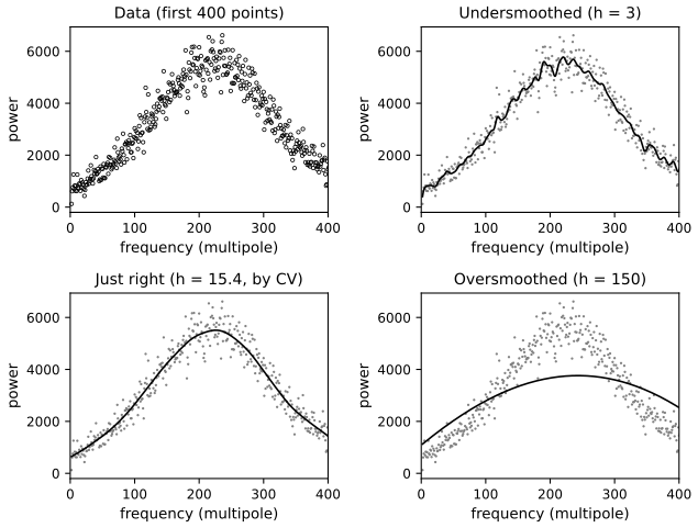
fig_4_5, local_linear_matrix, loocv_linear. Reproduces Wasserman (2006), Figure 4.5. Download: PDF · SVGExample 4.5: LIDAR and the regressogram
p. 48 In a light detection and ranging experiment, the response is the log ratio of the light received from two lasers, and the covariate is the distance travelled (range), for 221 observations. The regressogram cuts the covariate axis into bins of width \(h\) and averages the \(Y_i\) in each bin: it is the regression analogue of the histogram.
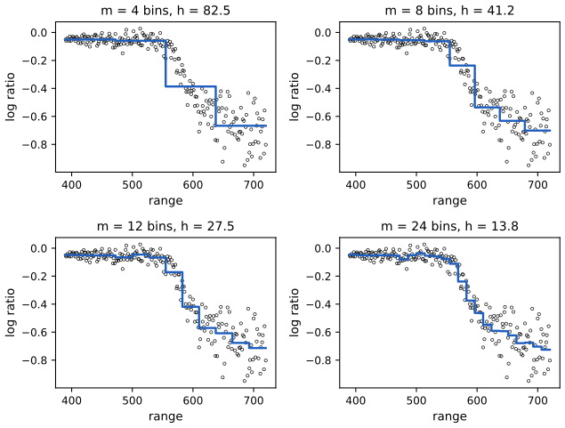
fig_4_6, regressogram. Reproduces Wasserman (2006), Figure 4.6. Download: PDF · SVGExample 4.6: bronchopulmonary dysplasia (binary regression)
pp. 48–49 For 223 babies, \(Y=1\) if the baby has bronchopulmonary dysplasia (BPD) and \(x\) is the birth weight in grams. Here \(r(x)=\P(Y=1\given X=x)\). The parametric benchmark is logistic regression,
\[ r(x;\beta_0,\beta_1)\equiv\P(Y=1\given X=x)=\frac{e^{\beta_0+\beta_1x}}{1+e^{\beta_0+\beta_1x}}, \]fitted by maximum likelihood; Newton's method gives \(\hat\beta_0=4.034\), \(\hat\beta_1=-0.00423\) per gram. Two nonparametric alternatives are a local linear regression of the 0/1 responses and local likelihood: at each \(x_0\), fit the logistic model with linear predictor \(a+b(x-x_0)\) by maximising the kernel-weighted log-likelihood \(\sum_iK((x_i-x_0)/h)\,\ell(a+b(x_i-x_0);Y_i)\), and report \(e^{\hat a}/(1+e^{\hat a})\). Local likelihood always gives a value in \([0,1]\); a local linear fit of 0/1 data need not.
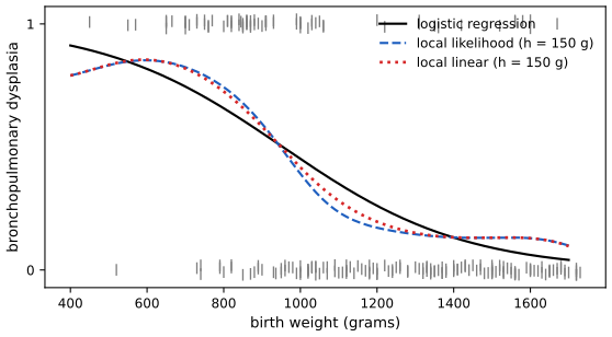
fig_4_7, logistic_irls, local_logistic. Reproduces Wasserman (2006), Figure 4.7. Download: PDF · SVGSee also (companion course): local likelihood in Statistical Learning: Theory and Methods.
Example 4.7: rock permeability (an additive model)
pp. 49–50 For 48 rock samples from a petroleum reservoir, the response is permeability and the covariates are the pore area, the pore perimeter and the shape (perimeter divided by the square root of area). A fully nonparametric model \(Y=r(x_1,x_2,x_3)+\epsilon\) is hard to fit with 48 points in three dimensions (Section 4.5); the additive model \(Y=\alpha+r_1(x_1)+r_2(x_2)+r_3(x_3)+\epsilon\) replaces one three-dimensional function by three one-dimensional ones. It is fitted by backfitting: cycle over \(j\), smoothing the partial residuals \(Y-\hat\alpha-\sum_{k\ne j}\hr_k(x_k)\) against \(x_j\) and centring the result, until nothing changes.
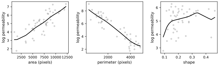
fig_4_8, backfit. Reproduces Wasserman (2006), Figure 4.8. Download: PDF · SVGFilling the gap 4.8: backfitting is a Gauss–Seidel iteration p. 50
The book shows the fitted components without saying how they are computed. Why does cycling over the components make sense?
Derivation
Let \(S_j\) be the \(n\times n\) smoothing matrix of the chosen smoother against \(x_j\), and \(\mathbf{f}_j=(r_j(x_{1j}),\dots,r_j(x_{nj}))^\T\). If each component were known except \(\mathbf{f}_j\), the natural estimate is \(\mathbf{f}_j=S_j(\mathbf{Y}-\alpha\mathbf{1}-\sum_{k\ne j}\mathbf{f}_k)\). Requiring this for all \(j\) at once gives the linear system
\[ \begin{pmatrix} I & S_1 & S_1\\ S_2 & I & S_2\\ S_3 & S_3 & I\end{pmatrix}\begin{pmatrix}\mathbf{f}_1\\ \mathbf{f}_2\\ \mathbf{f}_3\end{pmatrix}=\begin{pmatrix}S_1\\ S_2\\ S_3\end{pmatrix}(\mathbf{Y}-\alpha\mathbf{1}). \]Backfitting solves the \(j\)-th block row for \(\mathbf{f}_j\) using the newest values of the others: this is exactly the block Gauss–Seidel method. With \(\hat\alpha=\bar Y\), centring each \(\mathbf{f}_j\) removes the one obvious non-identifiability (constants can move between components). For symmetric smoothers with eigenvalues in \([0,1]\) (smoothing splines, for example) the iteration converges for any starting value; this is the theorem of Buja, Hastie and Tibshirani (1989). Local linear smoothers are not symmetric and there is no general guarantee, but on these data the iteration converged (largest change below \(10^{-10}\)) after 234 sweeps. ∎
See also (companion course): additive models and backfitting in Statistical Learning: Theory and Methods.
4.1 The Bias–Variance Tradeoff
See also (companion course): Section 20.1 of Probability and Statistical Inference, where the integrated decomposition is proved in full.
Definition 4.8 (loss, risk, integrated risk) pp. 50–52, (4.8), (4.9), (4.12), (4.13)
The squared error (or \(L_2\)) loss of \(\hf_n(x)\) as an estimate of \(f(x)\), and its average, the risk or mean squared error:
\[ L\big(f(x),\hf_n(x)\big)=\big(f(x)-\hf_n(x)\big)^2, \tag{4.8} \] \[ \mse=R\big(f(x),\hf_n(x)\big)=\E\Big(L\big(f(x),\hf_n(x)\big)\Big). \tag{4.9} \]The expectation is over the data, on which \(\hf_n\) depends. Over all \(x\): the integrated risk for densities and the average risk for regression,
\[ R(f,\hf_n)=\int R\big(f(x),\hf_n(x)\big)\,\d x, \tag{4.12} \] \[ R(r,\hr_n)=\frac1n\sum_{i=1}^nR\big(r(x_i),\hr_n(x_i)\big). \tag{4.13} \]Result 4.10 (risk = bias\(^2\) + variance; Exercise 4.2) p. 51, (4.10)–(4.11)
If \(\E\hf_n(x)^2\lt\infty\), then with \(\bias_x=\E(\hf_n(x))-f(x)\) and \(V_x=\V(\hf_n(x))\),
\[ R\big(f(x),\hf_n(x)\big)=\bias_x^2+V_x, \tag{4.10} \]in words, risk = mse = bias\(^2\) + variance (4.11). Integrating (by Tonelli's theorem, since everything is non-negative), \(R(f,\hf_n)=\int\bias_x^2\,\d x+\int V_x\,\d x\).
Result 4.14 (average risk and predictive risk) p. 53, (4.14)–(4.15)
Let \(Y_i^*=r(x_i)+\epsilon_i^*\) be new responses at the same \(x_i\), with \(\E\epsilon_i^*=0\) and the \(\epsilon_i^*\) independent of the data used to build \(\hr_n\). Then
\[ \E\Big(\frac1n\sum_{i=1}^n\big(Y_i^*-\hr_n(x_i)\big)^2\Big)=R(r,\hr_n)+c,\qquad c=\frac1n\sum_{i=1}^n\E\big((\epsilon_i^*)^2\big), \tag{4.14} \]and \(c=\sigma^2\) when every \(\epsilon_i^*\) has variance \(\sigma^2\) (4.15).
Filling the gap 4.1: proofs of (4.10) and (4.14), and the role of independence pp. 51–53
The book leaves (4.10) as Exercise 4.2 and states (4.14) after a one-line computation. Both rest on a cross term that vanishes, for different reasons.
Proof
(4.10). Fix \(x\) and write \(m=\E\hf_n(x)\). Then \(f(x)-\hf_n(x)=(f(x)-m)+(m-\hf_n(x))\), and squaring,
\[ \E\big(f(x)-\hf_n(x)\big)^2=(f(x)-m)^2+2(f(x)-m)\,\E\big(m-\hf_n(x)\big)+\E\big(m-\hf_n(x)\big)^2. \]The middle term is zero because \(f(x)-m\) is a constant and \(\E(m-\hf_n(x))=0\); the first term is \(\bias_x^2\) and the last is \(V_x\). The assumption \(\E\hf_n(x)^2\lt\infty\) makes every term finite.
(4.14). Expand \((Y_i^*-\hr_n(x_i))^2=(\epsilon_i^*)^2+2\epsilon_i^*\big(r(x_i)-\hr_n(x_i)\big)+\big(r(x_i)-\hr_n(x_i)\big)^2\). Because \(\epsilon_i^*\) is independent of \(\hr_n(x_i)\) and has mean zero, the cross term has expectation \(\E(\epsilon_i^*)\,\E(r(x_i)-\hr_n(x_i))=0\). Averaging over \(i\) gives (4.14). ∎
Why independence matters. If the same responses are used to fit and to evaluate (\(\epsilon_i^*=\epsilon_i\)), the cross term is \(-2\,\E(\epsilon_i\hr_n(x_i))=-2\cov(\epsilon_i,\hr_n(x_i))\), which is negative for every sensible smoother. For a linear smoother \(\hr_n(x_i)=\sum_jL_{ij}Y_j\) it equals \(-2\sigma^2L_{ii}\), so the training error underestimates the predictive risk by \(2\sigma^2\Tr(L)/n\) on average. This is why the risk must be estimated by cross-validation (or by adding back such a penalty), and why the leave-one-out scores of Figures 4.1, 4.3 and 4.5 leave each point out of its own fit.
When the data are oversmoothed the bias is large and the variance small; when undersmoothed, the reverse. Minimising the risk balances the two. The next example makes this exact.
Result 4.16 (Example 4.16: estimating \(f(0)\) by counting) pp. 53–55, (4.17)–(4.21)
Let \(p_h=\P(-h/2\lt X\lt h/2)=\int_{-h/2}^{h/2}f(x)\,\d x\), let \(N\) be the number of observations in \((-h/2,h/2)\), so \(N\sim\) Binomial\((n,p_h)\), and let
\[ \hf_n(0)=\frac{\hat p_h}{h}=\frac{N}{nh}. \tag{4.17} \]If \(f\) is twice continuously differentiable near 0, then as \(h\to0\),
\[ \bias=\E(\hf_n(0))-f(0)\approx\frac{f''(0)h^2}{24}, \tag{4.19} \] \[ \V(\hf_n(0))\approx\frac{f(0)}{nh}, \tag{4.20} \] \[ \mse\approx\frac{(f''(0))^2h^4}{576}+\frac{f(0)}{nh}\equiv Ah^4+\frac{B}{nh}. \tag{4.21} \](The book writes the count as \(X\); here it is \(N\) to avoid a clash with the observations.)
Filling the gap 4.2: Example 4.16 with exact formulas, remainders and the optimal width pp. 53–55
The book's derivation uses "\(\approx\)" three times and stops at (4.21). Here are the exact quantities, the size of each neglected term, the optimal \(h\) and the resulting rate, and what fails at a cusp.
Derivation
Exact formulas. Since \(N\sim\) Binomial\((n,p_h)\), \(\E N=np_h\) and \(\V N=np_h(1-p_h)\), so exactly
\[ \bias(h)=\frac{p_h}{h}-f(0),\qquad \V(\hf_n(0))=\frac{p_h(1-p_h)}{nh^2}. \]The bias. Assume \(f\) has a continuous second derivative on a neighbourhood of 0. Taylor's theorem with the Lagrange remainder gives, for \(|x|\le h/2\), \(f(x)=f(0)+xf'(0)+\tfrac12x^2f''(\xi_x)\) with \(\xi_x\) between 0 and \(x\). Integrating over \((-h/2,h/2)\), the linear term vanishes by symmetry and \(\int_{-h/2}^{h/2}x^2\,\d x=h^3/12\), so
\[ p_h=hf(0)+\frac{h^3}{24}f''(0)+\frac12\int_{-h/2}^{h/2}x^2\big(f''(\xi_x)-f''(0)\big)\,\d x. \]The last term is at most \(\tfrac{h^3}{24}\omega(h/2)\) in absolute value, where \(\omega(t)=\sup_{|u|\le t}|f''(u)-f''(0)|\to0\). Dividing by \(h\): \(\bias(h)=f''(0)h^2/24+o(h^2)\), which is (4.19). If \(f\) has four continuous derivatives the same argument with two more terms shows the error is \(O(h^4)\) (the cubic term also integrates to zero).
The variance. From the exact formula and \(p_h=hf(0)+O(h^3)\),
\[ \V(\hf_n(0))=\frac{p_h}{nh^2}-\frac{p_h^2}{nh^2}=\frac{f(0)}{nh}+O\Big(\frac hn\Big)-\frac{(f(0)+O(h^2))^2}{n}=\frac{f(0)}{nh}-\frac{f(0)^2}{n}+O\Big(\frac hn\Big). \]So (4.20) holds with a relative error \(O(h)\): the neglected \(-f(0)^2/n\) is smaller than the main term \(f(0)/(nh)\) by the factor \(hf(0)\). The book's intermediate expression \(f(0)/(nh)+f''(0)h/(24n)\) drops \(-f(0)^2/n\), which is of larger order than the term it keeps; the conclusion (4.20) is unaffected.
The optimal width. Write \(M(h)=Ah^4+B/(nh)\) with \(A=f''(0)^2/576\gt0\) and \(B=f(0)\gt0\). Then \(M'(h)=4Ah^3-B/(nh^2)\) vanishes only at
\[ h_*=\Big(\frac{B}{4An}\Big)^{1/5}=\Big(\frac{144\,f(0)}{f''(0)^2\,n}\Big)^{1/5}, \]and \(M\) is decreasing before and increasing after, so \(h_*\) is the minimiser. At \(h_*\) the identity \(4Ah_*^4=B/(nh_*)\) gives
\[ M(h_*)=Ah_*^4+4Ah_*^4=5Ah_*^4=\frac54\,B^{4/5}(4A)^{1/5}\,n^{-4/5}. \]At the optimum the squared bias is one quarter of the variance, and the mse decreases like \(n^{-4/5}\), slower than the \(n^{-1}\) of parametric problems. For the standard Normal density and \(n=10\,000\), \(h_*=0.515\); the exact mse, computed from the binomial formulas, is minimised at \(h=0.518\) (Figure 4.9).
Consistency. From the exact formulas, \(\hf_n(0)\to f(0)\) in mean square if and only if \(p_h/h\to f(0)\) and \(p_h(1-p_h)/(nh^2)\to0\); when \(f\) is continuous at 0 with \(f(0)\gt0\) this means \(h\to0\) and \(nh\to\infty\): the window must shrink, but more slowly than \(1/n\), so that it still catches infinitely many points.
Two cases outside the book's assumptions. (i) If \(f''(0)=0\) the leading bias is of order \(h^4\) and the best rate improves to \(n^{-8/9}\). (ii) If \(f\) has a cusp at 0, such as the Laplace density \(\tfrac12e^{-|x|}\), then \(p_h=1-e^{-h/2}\) and \(\bias(h)=(1-e^{-h/2})/h-\tfrac12=-h/8+O(h^2)\): the bias is of order \(h\), not \(h^2\). Then \(\mse\approx h^2/64+1/(2nh)\), the best width is \((16/n)^{1/3}\) and the best mse decreases only like \(n^{-2/3}\). Smoothness of the target, not the estimator, sets the rate; this theme returns in Chapters 7 to 9. ∎
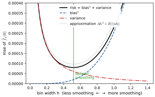
fig_4_9, ex416_exact. Reproduces Wasserman (2006), Figure 4.9. Download: PDF · SVGSee also (companion courses): the bias–variance demo of Bayesian and Probabilistic Machine Learning and Section 7.3 of Statistical Learning: Theory and Methods.
4.2 Kernels
Definition 4.22 (kernel) p. 55, (4.22)
A kernel is a smooth function \(K\) with
\[ K(x)\ge0,\qquad\int K(x)\,\d x=1,\qquad\int xK(x)\,\d x=0,\qquad\sigma_K^2\equiv\int x^2K(x)\,\d x\gt0. \tag{4.22} \]With \(I(x)=\I(|x|\le1)\), the standard examples are the boxcar \(\tfrac12I(x)\), the Gaussian \((2\pi)^{-1/2}e^{-x^2/2}\), the Epanechnikov \(\tfrac34(1-x^2)I(x)\) and the tricube \(\tfrac{70}{81}(1-|x|^3)^3I(x)\). (The boxcar is not smooth; the book includes it anyway.)
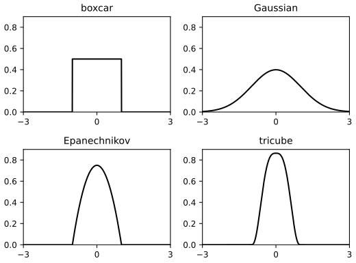
fig_4_10. Reproduces Wasserman (2006), Figure 4.10. Download: PDF · SVGKernels turn averages into local averages. Given pairs \((x_1,Y_1),\dots,(x_n,Y_n)\), the kernel-weighted average of the responses near \(x\) is
\[ \sum_{i=1}^nY_i\,\ell_i(x), \tag{4.23} \] \[ \ell_i(x)=\frac{K\big(\frac{x_i-x}{h}\big)}{\sum_{j=1}^nK\big(\frac{x_j-x}{h}\big)}. \tag{4.24} \]With the boxcar kernel this is the plain average of the \(Y_i\) with \(|x_i-x|\le h\); other kernels give weights that fade with distance, and smoother kernels give smoother estimates. Unlike the regressogram, whose bins are fixed in advance, the window moves with \(x\).
Filling the gap 4.3: the four kernels satisfy (4.22), their constants, and the local average as a least-squares fit pp. 55–56
The book lists the kernels without checking (4.22) or giving the two numbers that appear in every risk formula of later chapters: \(\sigma_K^2\) and \(R(K)=\int K^2\).
Derivation
Each kernel is even, so \(\int xK=0\) whenever \(\int|x|K\lt\infty\), which holds for all four. The integrals over \([-1,1]\) reduce to elementary ones on \([0,1]\) by symmetry.
Boxcar. \(\int_{-1}^1\tfrac12=1\), \(\sigma_K^2=\int_{-1}^1\tfrac12x^2=\tfrac13\), \(R(K)=\int_{-1}^1\tfrac14=\tfrac12\).
Gaussian. \(\int K=1\) and \(\sigma_K^2=1\) are the mean-zero, variance-one facts for \(\N(0,1)\); \(R(K)=\int\frac{1}{2\pi}e^{-x^2}\d x=\frac{\sqrt\pi}{2\pi}=\frac{1}{2\sqrt\pi}\approx0.2821\).
Epanechnikov. \(2\cdot\tfrac34\int_0^1(1-x^2)=\tfrac32\cdot\tfrac23=1\); \(\sigma_K^2=\tfrac32\int_0^1(x^2-x^4)=\tfrac32\big(\tfrac13-\tfrac15\big)=\tfrac15\); \(R(K)=2\cdot\tfrac{9}{16}\int_0^1(1-x^2)^2=\tfrac98\cdot\tfrac{8}{15}=\tfrac35\).
Tricube. Substitute \(u=x^3\), \(\d x=\tfrac13u^{-2/3}\d u\), so \(\int_0^1x^{a}(1-x^3)^b\,\d x=\tfrac13B\big(\tfrac{a+1}3,b+1\big)\) with \(B\) the beta function. Then
\[ \int_{-1}^1(1-|x|^3)^3\d x=\tfrac23B\big(\tfrac13,4\big)=\tfrac23\cdot\frac{\Gamma(\frac13)\,3!}{\Gamma(\frac{13}3)}=\tfrac23\cdot\frac{6}{\frac{10}3\cdot\frac73\cdot\frac43\cdot\frac13}=\frac{81}{70}, \]which is why the constant is \(70/81\). The same substitution gives \(\int_{-1}^1x^2(1-|x|^3)^3\d x=\tfrac23B(1,4)=\tfrac16\), so \(\sigma_K^2=\tfrac{70}{81}\cdot\tfrac16=\tfrac{35}{243}\approx0.1440\), and \(\int_{-1}^1(1-|x|^3)^6\d x=\tfrac23B(\tfrac13,7)=\tfrac{6561}{6916}\), so \(R(K)=\big(\tfrac{70}{81}\big)^2\tfrac{6561}{6916}=\tfrac{175}{247}\approx0.7085\).
| kernel | \(\sigma_K^2\) | \(R(K)=\int K^2\) | support |
|---|---|---|---|
| boxcar | 1/3 | 1/2 | \([-1,1]\) |
| Gaussian | 1 | \(1/(2\sqrt\pi)\) | \(\R\) |
| Epanechnikov | 1/5 | 3/5 | \([-1,1]\) |
| tricube | 35/243 | 175/247 | \([-1,1]\) |
All values were confirmed by numerical integration. Because \(\sigma_K\) differs between kernels, the same \(h\) means different amounts of smoothing for different kernels: a Gaussian with \(h=1\) is about as wide as an Epanechnikov kernel with \(h=\sqrt5\approx2.2\). That is why the cross-validated bandwidths of the local average demo differ between kernels while the fits look alike.
The local average is a least-squares fit. For fixed \(x\), the constant \(c\) that minimises \(\sum_iK((x_i-x)/h)(Y_i-c)^2\) solves \(\sum_iK((x_i-x)/h)(Y_i-c)=0\), i.e. \(c=\sum_i\ell_i(x)Y_i\), the estimate (4.23)–(4.24), provided the denominator in (4.24) is positive. Replacing the constant by a line \(a+b(x_i-x)\) gives the local linear estimator of Figure 4.5; this is the starting point of Chapter 5. The weights sum to one, \(\sum_i\ell_i(x)=1\), so a constant function is reproduced exactly. ∎
See also (companion courses): one-dimensional kernel smoothers in Statistical Learning: Theory and Methods, and the choice of kernel in Filling the gap 20.6 of Probability and Statistical Inference (the Epanechnikov kernel is optimal, but only slightly).
4.3 Which Loss Function?
p. 57 Instead of squared error one can use the \(L_p\) loss \(\big(\int|f(x)-\hf_n(x)|^p\d x\big)^{1/p}\). The \(L_1\) loss is resistant to outliers and invariant under one-to-one transformations, but for \(p\ne2\) the mathematics is much harder, so \(L_2\) remains the default. Another candidate is the Kullback–Leibler loss
\[ L(f,\hf_n)=\int f(x)\log\frac{f(x)}{\hf_n(x)}\,\d x, \]which maximum likelihood implicitly uses; but in smoothing it is dominated by the tails (Hall 1987). Both claims deserve a proof.
Filling the gap 4.4: why \(L_1\) is invariant, why maximum likelihood is Kullback–Leibler, and why the tails ruin it p. 57
Three statements made in one paragraph of the book.
Proof
(a) Invariance of \(L_1\). Let \(g\) be a strictly monotone, continuously differentiable map with inverse \(g^{-1}\), and let \(X\) have density \(f\). Then \(g(X)\) has density \(f_g(y)=f(g^{-1}(y))\,|(g^{-1})'(y)|\), and an estimate \(\hf\) transforms the same way. Changing variables \(y=g(x)\),
\[ \int|f_g(y)-\hf_g(y)|\,\d y=\int|f(g^{-1}(y))-\hf(g^{-1}(y))|\,|(g^{-1})'(y)|\,\d y=\int|f(x)-\hf(x)|\,\d x. \]For \(L_2\) the Jacobian appears squared inside the integral and only once in \(\d y\), so a factor \(|(g^{-1})'(y)|\) remains: \(\int(f_g-\hf_g)^2\d y=\int(f-\hf)^2(x)\,|g'(x)|^{-1}\d x\), which depends on \(g\). The \(L_1\) distance also has a scale-free interpretation (Scheffé's identity): \(\int|f-\hf|=2\sup_A|\int_Af-\int_A\hf|\), twice the largest difference in probability that the two densities give to any set.
(b) Maximum likelihood and KL. For a parametric family \(f_\theta\), \(\int f\log(f/f_\theta)=\int f\log f-\E_f\log f_\theta(X)\). The first term does not involve \(\theta\), and the average log-likelihood \(n^{-1}\sum_i\log f_\theta(X_i)\) estimates \(\E_f\log f_\theta(X)\) without bias. So maximising the likelihood is minimising an unbiased estimate of the KL loss, up to a constant.
(c) Tail sensitivity. The KL loss is infinite as soon as \(\hf_n=0\) on a set where \(f\gt0\), however small its probability. A kernel estimator with a compactly supported kernel is zero beyond \(\max_iX_i+h\), so its KL loss is infinite for every density with unbounded support. Even with a Gaussian kernel: if the truth is a Cauchy density, \(f(x)\sim1/(\pi x^2)\), the estimate has Gaussian tails, \(\log\hf_n(x)\approx-x^2/(2h^2)\), and the integrand \(f\log(f/\hf_n)\) behaves like \(1/(2\pi h^2)\) for large \(|x|\): it is not integrable, and the loss is infinite whatever the data. Its estimate by leave-one-out likelihood cross-validation is driven by the few most extreme observations, and the chosen bandwidth can be badly wrong for the bulk of the density; this is Hall's (1987) point. Squared error and \(L_1\) loss weight the tails by the (tiny) densities themselves and do not have this problem. ∎
How the three losses relate to each other is the subject of Exercise 4.5.
4.4 Confidence Sets
p. 57 An estimate without a measure of its uncertainty is of limited use. Later chapters construct confidence sets of two kinds: a ball
\[ B_n=\Big\{f:\int\big(f(x)-\hf_n(x)\big)^2\d x\le s_n^2\Big\} \]with radius \(s_n\), or a band (envelope) \(B_n=\{f:\ell(x)\le f(x)\le u(x)\text{ for all }x\}\) given by two functions \(\ell\le u\). Either way one wants
\[ \P_f(f\in B_n)\ge1-\alpha\quad\text{for all }f\in\F, \tag{4.25} \]for some large class \(\F\) of functions; in practice (4.25) often holds only approximately, for instance as \(n\to\infty\).
Filling the gap 4.5: pointwise versus uniform coverage, bands versus balls pp. 57
Two remarks that the book's short section takes for granted, and that recur in Chapters 5 to 9.
Proof
A band gives a ball. Suppose \(\ell\le\hf_n\le u\) and \(\P_f(\ell\le f\le u\text{ everywhere})\ge1-\alpha\). On that event \(|f(x)-\hf_n(x)|\le w(x)\equiv\max\{u(x)-\hf_n(x),\hf_n(x)-\ell(x)\}\) for every \(x\), so \(\int(f-\hf_n)^2\le\int w^2\). Hence the ball with \(s_n^2=\int w^2\) has coverage at least \(1-\alpha\) too. The converse fails: an \(L_2\) ball contains functions with arbitrarily tall narrow spikes, so it does not bound \(f(x)\) at any single \(x\).
"For all \(x\)" matters. If for each fixed \(x\) an interval \(C(x)\) has \(\P(f(x)\in C(x))\ge1-\alpha\), the intervals together need not cover the whole curve with probability \(1-\alpha\). At \(m\) points, the union bound gives \(\P(f(x_j)\notin C(x_j)\text{ for some }j)\le\sum_j\P(f(x_j)\notin C(x_j))\), so intervals at level \(1-\alpha/m\) each give simultaneous coverage \(\ge1-\alpha\) at the \(m\) points (Bonferroni). Passing from a grid to all \(x\) needs control of the curve between grid points, which is what the tube formulas and the effective number of independent windows of later chapters supply.
"For all \(f\in\F\)" matters. Coverage uniformly over a class is much harder than coverage at each fixed \(f\). A band centred at \(\hf_n\) with width proportional to its standard deviation covers \(\E\hf_n\), not \(f\); the difference is the bias, which is unknown and can be as large as the width for some \(f\) in the class. The usual remedies (undersmoothing, bias correction, or covering a smoothed version of \(f\)) are discussed in Chapter 5. ∎
See also (companion course): the confidence envelope for a histogram and the band for kernel regression in Probability and Statistical Inference, Theorem 20.10 and the kernel regression band demo.
4.5 The Curse of Dimensionality
pp. 58–59 Bellman's (1961) phrase covers two things: the computational curse, where the cost of a method grows exponentially with the dimension \(d\), and the statistical curse, the subject here: the sample size needed for a given accuracy grows exponentially with \(d\). The reason is that smoothing averages over a neighbourhood of \(x\), and in high dimensions neighbourhoods are empty unless they are large. The book states that for twice-differentiable targets the mse of a nonparametric estimator typically behaves like \(c\,n^{-4/(4+d)}\), and gives a counting example.
Filling the gap 4.6: where \(n^{-4/(4+d)}\) comes from, the sample size it implies, and the counting example pp. 58–59
The book quotes the rate from later chapters, solves for \(n\) with a slip in the exponent, and computes a volume with a misprinted cube. Here is the full argument.
Derivation
The rate. Estimate \(f(0)\) for a density on \(\R^d\) by counting the points in the cube \(Q_h=[-h/2,h/2]^d\): \(\hf_n(0)=N/(nh^d)\). This is Example 4.16 in \(d\) dimensions, worked out in Exercise 4.6: the bias is \(h^2\Delta f(0)/24+o(h^2)\) (\(\Delta\) the Laplacian) and the variance is \(f(0)/(nh^d)\,(1+O(h))\). The bias does not depend on \(d\) but the variance does: a cube of side \(h\) has volume \(h^d\), so it holds about \(nh^df(0)\) points. Minimising \(Ah^4+B/(nh^d)\) gives \(h_*\propto n^{-1/(4+d)}\) and
\[ \mse(h_*)=\Big(1+\frac4d\Big)Ah_*^4=C_d\,n^{-4/(4+d)}. \]That no estimator can do better, uniformly over the class of densities with bounded second derivatives, is a minimax lower bound proved later in the course (Stone 1980).
The sample size. Setting \(c\,n^{-4/(4+d)}=\delta\) and solving,
\[ n=\Big(\frac c\delta\Big)^{(4+d)/4}, \]not \((c/\delta)^{d/4}\) as printed. The two differ by the factor \(c/\delta\), which does not depend on \(d\), so the book's conclusion stands: the exponent grows linearly in \(d\) and \(n\) grows exponentially. Compare a parametric model, where \(\mse\approx c/n\) and \(n=c/\delta\) in every dimension. Concretely, for the counting estimator and the standard Normal density in \(d\) dimensions, a relative mse \(\mse/f(0)^2=0.1\) requires about 17 observations in one dimension, 440 in four, 6600 in six and 3.2 million in ten (Exercise 4.6).
The counting example. For \(n\) points uniform on \([-1,1]\), the interval \([-0.1,0.1]\) has probability \(0.2/2=0.1\) and holds about \(n/10\) points. For points uniform on the cube \([-1,1]^{10}\) (the book writes \([0,1]^{10}\), which does not contain \([-0.1,0.1]^{10}\); the formula it uses is the one for \([-1,1]^{10}\)), the sub-cube \([-0.1,0.1]^{10}\) has probability \((0.2/2)^{10}=10^{-10}\). Even a billion points leave it empty with probability \((1-10^{-10})^{10^9}\approx e^{-0.1}\approx0.90\).
Neighbourhoods are not local. Turning the question round: to hold a fraction \(q\) of uniform data, a sub-cube of \([-1,1]^d\) needs half-width \(q^{1/d}\). For \(q=1\%\) and \(d=10\) that is \(0.01^{1/10}=0.63\): the "neighbourhood" spans 63% of the range of every coordinate, and an average over it is no longer local, so its bias is large. Similarly, for \(n\) points uniform in the unit ball of \(\R^d\), \(\P(\text{all points farther than }t\text{ from the centre})=(1-t^d)^n\), so the median distance from the centre to the nearest point is \((1-2^{-1/n})^{1/d}\): for \(n=500\) and \(d=10\) it is 0.52, more than half-way to the boundary. ∎
The conclusion of the book is worth repeating: a smoother can be computed in high dimensions, but it will not be accurate, and an honest confidence set will be very wide. That is a correct statement about the difficulty of the problem, not a failure of the method. Structure (additivity as in Example 4.7, sparsity, low intrinsic dimension) is what makes high-dimensional smoothing possible.
See also (companion course): local methods in high dimensions in Statistical Learning: Theory and Methods, with its curse of dimensionality demo.
4.6 Bibliographic Remarks
p. 59 Book-length treatments of smoothing include Silverman (1986), Scott (1992), Simonoff (1996), Fan and Gijbels (1996) and Ruppert, Wand and Carroll (2003). Hall (1987) discusses the problems of Kullback–Leibler loss, and Hastie, Tibshirani and Friedman (2001) discuss the curse of dimensionality at length. Full entries are in the references.
4.7 Exercises
All 7 exercises of Chapter 4 (Wasserman 2006, pp. 59–60), restated in my own words, with complete solutions (hidden).
Exercise 4.1. Let \(X_1,\dots,X_n\) be iid with density \(f\), and let the likelihood of \(f\) be \(L_n(f)=\prod_{i=1}^nf(X_i)\). If the model is the set of all probability densities, what is the maximum likelihood estimator of \(f\)?
Solution
There is none: the likelihood is unbounded. Assume the \(X_i\) are distinct (which happens with probability one). For \(\varepsilon\gt0\) let \(f_\varepsilon(x)=\frac1n\sum_{j=1}^n\varepsilon^{-1}\phi((x-X_j)/\varepsilon)\), a density. Keeping only the \(j=i\) term,
\[ L_n(f_\varepsilon)=\prod_{i=1}^nf_\varepsilon(X_i)\ge\prod_{i=1}^n\frac{1}{n\varepsilon\sqrt{2\pi}}=\big(n\varepsilon\sqrt{2\pi}\big)^{-n}\to\infty\quad(\varepsilon\to0). \]So \(\sup_fL_n(f)=\infty\) and no density attains it. The maximising sequence concentrates on the data and converges (weakly) to the empirical distribution \(\hat P_n=\frac1n\sum_i\delta_{X_i}\), which has no density: unrestricted maximum likelihood "estimates" \(f\) by spikes at the observations, the ultimate undersmoothed estimate. This is why density estimation needs a smoothing parameter, or a restriction of the model (bounded densities, monotone densities, log-concave densities, or a penalty on roughness), before likelihood methods can work.
Exercise 4.2. Prove (4.10).
Solution
See the proof in Filling the gap 4.1: add and subtract \(m=\E\hf_n(x)\), expand the square, and note that the cross term \(2(f(x)-m)\E(m-\hf_n(x))\) is zero. The integrated version follows by integrating over \(x\).
Exercise 4.3. Let \(X_1,\dots,X_n\) be iid \(\N(\theta,1)\) with density \(f_\theta(x)=(2\pi)^{-1/2}e^{-(x-\theta)^2/2}\), and estimate the density by the plug-in \(\hf(x)=f_{\hat\theta}(x)\) with \(\hat\theta=\bar X_n\). Find its risk.
Solution
Use the integrated squared error risk (4.12). Two Gaussian identities do all the work: for constants \(a,b\), \(\int\phi(x-a)\phi(x-b)\,\d x=\frac{1}{2\sqrt\pi}e^{-(a-b)^2/4}\) (the density of \(\N(0,2)\) at \(a-b\)), and for \(D\sim\N(0,s^2)\) and \(c\gt0\), \(\E e^{-cD^2}=(1+2cs^2)^{-1/2}\). With \(D=\hat\theta-\theta\),
\[ \int(f_{\hat\theta}-f_\theta)^2=\int\phi^2+\int\phi^2-2\int\phi(x-\hat\theta)\phi(x-\theta)\,\d x=\frac{1}{\sqrt\pi}\Big(1-e^{-D^2/4}\Big). \]Since \(D\sim\N(0,1/n)\), \(\E e^{-D^2/4}=(1+\frac{1}{2n})^{-1/2}\), and
\[ R(f_\theta,\hf)=\frac{1}{\sqrt\pi}\Big(1-\big(1+\tfrac1{2n}\big)^{-1/2}\Big)=\frac{1}{4\sqrt\pi\,n}+O(n^{-2}). \](The first-order term: \(1-(1+u)^{-1/2}=u/2+O(u^2)\) with \(u=1/(2n)\).) For \(n=10\) the formula gives 0.013597; a simulation of 200 000 data sets gave the same value to three digits. The risk falls like \(1/n\): when the parametric model is right, the plug-in estimator beats every nonparametric density estimator, whose risk falls like \(n^{-4/5}\) at best. The price is that if the model is wrong, the risk does not go to zero at all.
For the risk at a single point the same method gives \(\E(\phi(x-\hat\theta)-\phi(x-\theta))^2\) in closed form; to first order it is \(\phi(x-\theta)^2(x-\theta)^2/n\) by the delta method, which vanishes at \(x=\theta\) where the density is flat in \(\theta\).
Exercise 4.4. The Kullback–Leibler distance between densities \(f\) and \(g\) is \(D(f,g)=\int f\log(f/g)\). In a one-parameter model \(\{f_\theta:\theta\in\R\}\), show that \(D(f_\theta,f_\psi)\approx(\theta-\psi)^2I(\theta)/2\) for \(\psi\) close to the true value \(\theta\), where \(I(\theta)\) is the Fisher information.
Solution
Assume the usual regularity conditions: the support of \(f_\psi\) does not depend on \(\psi\), \(\log f_\psi(x)\) is three times differentiable in \(\psi\), and differentiation under the integral sign is allowed (dominated by an integrable function near \(\theta\)). Let \(g(\psi)=D(f_\theta,f_\psi)=\int f_\theta\log f_\theta-\int f_\theta\log f_\psi\). Then \(g(\theta)=0\),
\[ g'(\psi)=-\int f_\theta(x)\,\frac{\partial}{\partial\psi}\log f_\psi(x)\,\d x,\qquad g'(\theta)=-\E_\theta[s_\theta(X)]=0, \]because the score \(s_\theta=\partial_\theta\log f_\theta\) has mean zero (\(\int\partial_\theta f_\theta=\partial_\theta\int f_\theta=0\)). Next \(g''(\theta)=-\E_\theta[\partial_\theta^2\log f_\theta(X)]=I(\theta)\), the information identity. Taylor's theorem gives
\[ D(f_\theta,f_\psi)=\tfrac12I(\theta)(\psi-\theta)^2+O(|\psi-\theta|^3). \]So near the truth the KL loss of a parameter estimate is half the Fisher-weighted squared error: it is an \(L_2\) loss on the parameter, measured in the metric in which the parameter is hard to estimate. For \(\N(\theta,1)\) the relation is exact, \(D=(\theta-\psi)^2/2\); for the exponential density \(\theta e^{-\theta x}\), \(D=\log(\theta/\psi)+\psi/\theta-1\) and \(I(\theta)=1/\theta^2\), and the ratio of the two sides tends to 1 as \(\psi\to\theta\) (it is 0.987 at \(\psi=1.02\theta\)). The Fisher information is defined and discussed in Section 9.7 of the companion course.
Exercise 4.5. What is the relationship between \(L_1\) loss, \(L_2\) loss and Kullback–Leibler loss?
Solution
Write \(\|f-g\|_1=\int|f-g|\), \(\|f-g\|_2^2=\int(f-g)^2\) and \(D(f,g)=\int f\log(f/g)\) for densities \(f,g\).
(i) KL controls \(L_1\) (Pinsker's inequality): \(\|f-g\|_1\le\sqrt{2D(f,g)}\). Proof. Let \(A=\{f\gt g\}\), \(p=\int_Af\), \(q=\int_Ag\); then \(\|f-g\|_1=2(p-q)\) (Scheffé). By the log-sum inequality applied on \(A\) and on \(A^c\), \(D(f,g)\ge p\log\frac pq+(1-p)\log\frac{1-p}{1-q}\equiv d(p,q)\). For fixed \(p\), \(k(q)=d(p,q)-2(p-q)^2\) has \(k(p)=0\) and \(k'(q)=(q-p)\big(\frac{1}{q(1-q)}-4\big)\), which is \(\le0\) for \(q\le p\) because \(q(1-q)\le\frac14\). So \(k(q)\ge0\) for \(q\le p\), i.e. \(D\ge d(p,q)\ge2(p-q)^2=\tfrac12\|f-g\|_1^2\). The converse fails: \(D\) can be infinite while \(\|f-g\|_1\) is tiny (Filling the gap 4.4).
(ii) \(L_2\) controls KL when \(g\) is bounded below: since \(\log u\le u-1\),
\[ D(f,g)=\int f\log\frac fg\le\int f\Big(\frac fg-1\Big)=\int\frac{(f-g)^2}{g}\le\frac{\|f-g\|_2^2}{\inf_xg(x)}, \]the middle term being the \(\chi^2\) distance (the identity uses \(\int f=\int g=1\)).
(iii) \(L_1\) versus \(L_2\): \(\|f-g\|_2^2\le\|f-g\|_\infty\|f-g\|_1\le(\sup f+\sup g)\|f-g\|_1\), and if both densities live on an interval of length \(\ell\), Cauchy–Schwarz gives \(\|f-g\|_1\le\sqrt\ell\,\|f-g\|_2\).
Summary. For densities on a bounded set, bounded above and below, all three losses are equivalent up to constants and squares: \(\tfrac12\|f-g\|_1^2\le D\le\|f-g\|_2^2/\inf g\) and \(\|f-g\|_1\le\sqrt\ell\|f-g\|_2\). Without those conditions, \(L_1\) is the weakest requirement (always finite, at most 2), \(L_2\) can be infinite for unbounded densities, and KL can be infinite because of the tails. For two Normal densities \(\N(0,1)\) and \(\N(0.5,1)\): \(\|f-g\|_1=0.3949\), \(\sqrt{2D}=0.5\), and \(\|f-g\|_2^2=0.0342\); the inequalities were confirmed numerically for this and other pairs.
Exercise 4.6. Repeat the derivation leading to (4.21) for \(d\)-dimensional \(X\), using a small \(d\)-dimensional cube instead of \([-h/2,h/2]\). Find the \(h\) that minimises the mse, and how large \(n\) must be for the mse to equal 0.1.
Solution
Let \(Q_h=[-h/2,h/2]^d\), \(p_h=\int_{Q_h}f\), \(N\sim\) Binomial\((n,p_h)\) the number of points in \(Q_h\), and \(\hf_n(0)=N/(nh^d)\). Assume \(f\) has continuous second partial derivatives near 0.
Bias. Taylor: \(f(x)=f(0)+\nabla f(0)^\T x+\tfrac12x^\T Hx+o(\|x\|^2)\), \(H\) the Hessian at 0. Over the symmetric cube, \(\int_{Q_h}x_j=0\), \(\int_{Q_h}x_jx_k=0\) for \(j\ne k\), and \(\int_{Q_h}x_j^2=h^{d-1}\cdot h^3/12=h^{d+2}/12\). Hence
\[ p_h=h^df(0)+\frac{h^{d+2}}{24}\Delta f(0)+o(h^{d+2}),\qquad\bias=\frac{p_h}{h^d}-f(0)=\frac{h^2}{24}\Delta f(0)+o(h^2), \]with \(\Delta f(0)=\sum_jf_{jj}(0)\) the Laplacian.
Variance. \(\V\hf_n(0)=p_h(1-p_h)/(nh^{2d})=f(0)/(nh^d)\,\big(1+O(h^2)+O(h^d)\big)\).
Optimum. \(\mse\approx Ah^4+B/(nh^d)\) with \(A=(\Delta f(0))^2/576\), \(B=f(0)\). Setting the derivative \(4Ah^3-dB/(nh^{d+1})\) to zero,
\[ h_*=\Big(\frac{dB}{4An}\Big)^{1/(4+d)},\qquad\mse(h_*)=\Big(1+\frac4d\Big)Ah_*^4=c_d\,n^{-4/(4+d)}, \]where \(c_d=(1+4/d)A\,(dB/(4A))^{4/(4+d)}\). For \(d=1\) this is Filling the gap 4.2.
Sample size. \(\mse(h_*)=\delta\) when \(n=(c_d/\delta)^{(4+d)/4}\). With absolute mse 0.1 the answer depends on the scale of \(f\) and is meaningless for many densities: for the standard Normal density in \(d\) dimensions, \(f(0)=(2\pi)^{-d/2}\) and \(f(0)^2\lt0.1\) already, so the trivial estimate 0 has mse below 0.1 and the formula returns \(n\lt1\) for \(d\ge2\). A meaningful target is a relative mse, \(\mse/f(0)^2=0.1\). For the standard Normal, \(\Delta f(0)=-d\,f(0)\), and the required \(n\) is:
\(d\) 1 2 3 4 5 6 8 10 \(n\) for relative mse 0.1 17 43 129 439 1635 6593 129 879 3 156 685 \(n\) for relative mse 0.01 302 1360 7272 43 865 290 817 2 084 840 1.3e8 1.0e10 These are first-order approximations (for large \(d\) the optimal cube is not small, and higher-order terms make the true numbers larger), but the exponential growth is unmistakable: each extra dimension multiplies \(n\) by a factor between about 2.5 and 5 here, and a tenfold gain in accuracy costs a factor \(10^{(4+d)/4}\).
Exercise 4.7. Download the data sets of this chapter from the book's website, write programs for histograms and regressograms, and try them on the data.
Solution
The functions
hist_counts,hist_cv,regressogramandregressogram_loocvin the chapter's code do this, with the number of bins chosen by leave-one-out cross-validation (for the regressogram: the average squared error of predicting each \(Y_i\) by the mean of the other points in its bin; points alone in their bin are skipped).- Galaxy redshifts (histogram on \([0,0.2]\), \(n=1266\)): the score is minimised at 258 bins (width 0.00078); it is within 3% of its minimum for every number of bins from 80 to 335 (Figure 4.1).
- LIDAR (regressogram, \(n=221\)): 14 bins of width 23.6, with leave-one-out mean squared error 0.00707, compared with a response variance of 0.0794.
- CMB, first 400 points (regressogram): 21 bins of width 19, with leave-one-out mean squared error \(1.78\times10^5\), against a response variance of \(2.60\times10^6\) (the local linear fit of Figure 4.5 does slightly better, \(1.72\times10^5\)).
- BPD (regressogram of a 0/1 response, \(n=223\)): the score is very flat and noisy (between 0.158 and 0.18 for almost every number of bins from 2 to 60), so its minimiser (43 bins) means little. A binary response carries little information about the shape of \(r\), and a smooth parametric or local likelihood fit is preferable here (Figure 4.7).
▶ DemoBPD as a local proportionRegressograms and kernel averages of all three regression data sets, with the cross-validation score.
Filling the gap 4.7: the three cross-validation scores used in Figures 4.1, 4.3 and 4.5 pp. 44–47
The book calls the lower right panels of Figures 4.1 and 4.3 "estimated mse" and defers the details to Chapters 5 and 6. Here is what was computed, and why each formula is right. In each case the score estimates the risk up to a term that does not depend on the smoothing parameter.
Derivation
Densities. The integrated risk is \(\int(\hf_n-f)^2=\int\hf_n^2-2\int\hf_nf+\int f^2\). The last term does not depend on \(h\), and \(\int\hf_nf=\E_X[\hf_n(X)]\) for a new \(X\sim f\), which is estimated by \(n^{-1}\sum_i\hf_{(-i)}(X_i)\), with \(\hf_{(-i)}\) built without \(X_i\). So the score is
\[ \hat J(h)=\int\hf_n^2-\frac2n\sum_{i=1}^n\hf_{(-i)}(X_i), \]and \(\E\hat J(h)=\E\int(\hf_n-f)^2-\int f^2\) up to the difference between \(n\) and \(n-1\) points. Histogram, \(m\) bins of width \(h\) with proportions \(\hat p_j\): the score simplifies to \(\hat J(h)=\frac{2}{(n-1)h}-\frac{n+1}{(n-1)h}\sum_j\hat p_j^2\); the proof is in Filling the gap 20.4 of the companion course, and the formula was checked against the definition. Gaussian kernel: \(\int\phi_h(x-a)\phi_h(x-b)\,\d x=\phi_{h\sqrt2}(a-b)\) (the convolution of two Normal densities), so
\[ \int\hf_n^2=\frac{1}{n^2}\sum_{i,j}\phi_{h\sqrt2}(X_i-X_j),\qquad\hf_{(-i)}(X_i)=\frac{1}{n-1}\sum_{j\ne i}\phi_h(X_i-X_j), \]with \(\phi_s\) the \(\N(0,s^2)\) density; the score needs only the \(n^2\) pairwise differences.
Regression with a local linear smoother. The score is \(n^{-1}\sum_i(Y_i-\hr_{(-i)}(x_i))^2\), whose expectation is the predictive risk (4.14) of the fit from \(n-1\) points. It needs only one fit: if \(\hr_n(x_i)=\sum_jL_{ij}Y_j\) is the local linear smoother, then
\[ Y_i-\hr_{(-i)}(x_i)=\frac{Y_i-\hr_n(x_i)}{1-L_{ii}}. \]Proof. At the target \(x_i\), \(\hr_n(x_i)=e_1^\T(X^\T WX)^{-1}X^\T WY\), where row \(j\) of \(X\) is \((1,x_j-x_i)\) and \(W=\diag(K((x_j-x_i)/h))\). Write \(z=(1,0)^\T\), the row of \(X\) for \(j=i\), and \(w=K(0)\), its weight. Deleting point \(i\) replaces \(G=X^\T WX\) by \(G-wzz^\T\) and \(X^\T WY\) by \(X^\T WY-wzY_i\). By the Sherman–Morrison formula, \((G-wzz^\T)^{-1}=G^{-1}+\frac{wG^{-1}zz^\T G^{-1}}{1-wz^\T G^{-1}z}\). Note \(L_{ii}=wz^\T G^{-1}z\) and \(\hr_n(x_i)=z^\T G^{-1}X^\T WY\). Multiplying out,
\[ \hr_{(-i)}(x_i)=z^\T(G-wzz^\T)^{-1}(X^\T WY-wzY_i)=\frac{\hr_n(x_i)-L_{ii}Y_i}{1-L_{ii}}, \]and \(Y_i-\hr_{(-i)}(x_i)=(Y_i-\hr_n(x_i))/(1-L_{ii})\). The same argument covers any local polynomial fit, and the kernel local average (4.23)–(4.24) is the constant case. The shortcut agreed with brute-force refitting to machine precision on the CMB data. ∎
Notes on the book
The book's website has no errata list. The points below are mine, each with the evidence.
Figure 4.8 (p. 52): the panels plot shifted columns of the rock data
The data file has columns area, perimeter, shape and permeability, with ranges 1016–12212, 308–4864, 0.090–0.464 and 6.3–1300. The book's panels are labelled area, perimeter and shape with horizontal ranges of about 1000–5000, 0.1–0.4 and 0–1000, and a vertical axis "log permeability" running from 7 to 9. These ranges match perimeter, shape and permeability on the horizontal axes, and \(\log(\text{area})\) (6.9 to 9.4) on the vertical axis, much better than the labelled variables (log permeability runs from 1.8 to 7.2). It appears that the columns were read one place off. Figure 4.8 above uses the variables the text describes.
Page 58: the sample size is \((c/\delta)^{(4+d)/4}\), not \((c/\delta)^{d/4}\)
Solving \(c\,n^{-4/(4+d)}=\delta\) gives \(n=(c/\delta)^{(4+d)/4}\). The printed exponent \(d/4\) drops a factor \(c/\delta\) that does not depend on \(d\), so the conclusion (exponential growth in \(d\)) is unaffected (Filling the gap 4.6).
Page 58: the cube \([0,1]^{10}\) should be \([-1,1]^{10}\)
The example puts the points in \([0,1]^{10}\) and counts those in \([-0.1,0.1]^{10}\), which is not inside \([0,1]^{10}\). The fraction \((0.2/2)^{10}\) used in the book is the one for points uniform on \([-1,1]^{10}\), consistent with the one-dimensional example on \([-1,1]\). (For \([0,1]^{10}\) and the corner cube \([0,0.1]^{10}\) the answer is the same \(10^{-10}\).) Also on that page, "the mean squared of any nonparametric estimator" is missing the word "error".
Page 55, (4.20): a dropped term of larger order
The middle expression of (4.20), \(f(0)/(nh)+f''(0)h/(24n)\), keeps a term of order \(h/n\) but drops \(-p_h^2/(nh^2)=-f(0)^2/n+O(h^2/n)\), which is of larger order. Both are negligible next to \(f(0)/(nh)\), so the final approximation is right (Filling the gap 4.2).
Pages 44 and 56: two small differences
Example 4.3 says the cross-validated histogram has 308 bins; with the score of Filling the gap 4.7 on \([0,0.2]\) the minimiser is 258, and 308 is inside the flat region of the score (Figure 4.1), so the difference is within the noise of the criterion and may come from a different bin grid. In (4.24) the kernel is evaluated at \((X_i-x)/h\) with a capital \(X\), although the covariates were written \(x_i\) in (4.23); the two mean the same.
Demonstrations for this chapter
Each demonstration runs in the browser, with seeded random numbers where there is randomness, and links back to these notes. The ▶ Demo boxes above open them already set to the case under discussion.
| Demonstration | What you can see | Sections and results |
|---|---|---|
| The bias–variance trade-off at a point | The counting estimator of \(f(0)\) for a Normal, a bimodal and a Laplace density: the exact distribution of the estimate, the exact squared bias, variance and mse against \(h\), the approximation \(Ah^4+B/(nh)\) and the optimal width, for \(n\) from 10 to a million. Presets: 1 Figure 4.9; 2 undersmoothing; 3 oversmoothing; 4 more data; 5 a cusp. | 4.1; Result 4.16, Filling the gap 4.2 |
| Regressograms and kernel local averages | The LIDAR, CMB and BPD data with a regressogram or a boxcar, Gaussian, Epanechnikov or tricube local average; the weights at a chosen point; the leave-one-out score against \(h\). Presets: 1 Figure 4.6; 2 boxcar; 3 tricube; 4 CMB undersmoothed; 5 BPD. | Examples 4.4–4.6, 4.2; Filling the gaps 4.3, 4.7, Exercise 4.7 |
| The curse of dimensionality | Simulated uniform points in up to 20 dimensions: how many fall in a small cube, the width needed to hold a fixed fraction, and the sample size for a relative mse \(\delta\) from Exercise 4.6. Presets: 1 one dimension; 2 ten dimensions; 3 non-local neighbourhoods; 4 sample sizes; 5 ten times the accuracy. | 4.5; Filling the gap 4.6, Exercise 4.6 |
The Python code that produces every figure of this page is code/ch04_smoothing_concepts.py (see the code index).
References
- Wasserman, L. (2006). All of Nonparametric Statistics. Springer, New York. Chapter 4, pp. 43–60. www.stat.cmu.edu/~larry/all-of-nonpar.
- Bellman, R. (1961). Adaptive Control Processes: A Guided Tour. Princeton University Press.
- Buja, A., Hastie, T. and Tibshirani, R. (1989). Linear smoothers and additive models. Annals of Statistics, 17(2), 453–510.
- Fan, J. and Gijbels, I. (1996). Local Polynomial Modelling and Its Applications. Chapman and Hall, London.
- Hall, P. (1987). On Kullback–Leibler loss and density estimation. Annals of Statistics, 15(4), 1491–1519.
- Hastie, T., Tibshirani, R. and Friedman, J. (2001). The Elements of Statistical Learning. Springer, New York.
- Pagano, M. and Gauvreau, K. (1993). Principles of Biostatistics. Duxbury Press, Belmont.
- Ruppert, D., Wand, M. P. and Carroll, R. J. (2003). Semiparametric Regression. Cambridge University Press.
- Scott, D. W. (1992). Multivariate Density Estimation: Theory, Practice, and Visualization. Wiley, New York.
- Silverman, B. W. (1986). Density Estimation for Statistics and Data Analysis. Chapman and Hall, London.
- Simonoff, J. S. (1996). Smoothing Methods in Statistics. Springer, New York.
- Stone, C. J. (1980). Optimal rates of convergence for nonparametric estimators. Annals of Statistics, 8(6), 1348–1360.
- Venables, W. N. and Ripley, B. D. (2002). Modern Applied Statistics with S, 4th edition. Springer, New York.
The numerical statements in the text (the cross-validated bin numbers and bandwidths, the kernel constants, the exact and approximate bias–variance curves, the leave-one-out shortcut, the risk in Exercise 4.3, the inequalities of Exercise 4.5 and the sample sizes of Exercise 4.6) were confirmed numerically.