Estimating the cdf and Statistical Functionals
Before densities and regression functions, the simplest nonparametric object: the distribution function itself. The empirical cdf estimates it at the parametric rate \(1/\sqrt n\), uniformly in \(x\) and with an explicit, distribution-free confidence band. Most quantities of interest (means, variances, quantiles, correlations) are functionals \(T(F)\) of the cdf, estimated by plugging in the empirical cdf; their standard errors come from a derivative of \(T\), the influence function, which turns a nonlinear estimator into an average plus a small remainder. The chapter closes with Vapnik–Chervonenkis theory, which extends the uniform control of the empirical cdf from half-lines to any class of sets of finite combinatorial complexity.
Ch. 1 Introduction Ch. 2 The cdf and functionals Ch. 3 Bootstrap and jackknife Ch. 4 Smoothing Ch. 5 Regression Ch. 6 Density estimation Ch. 7 Normal means and minimax Ch. 8 Orthogonal functions Ch. 9 Wavelets Ch. 10 Other topics
How to read these notes
They follow the book. Sections carry the book's numbers (2.1 to 2.7), results keep the book's numbering (Theorem 2.4, Example 2.35, ...), and displayed equations that appear in the book carry its equation numbers, e.g. \((2.5)\). Unnumbered equations are steps the book leaves out.
Filling the gaps. Wherever the book states a result without proof, quotes it from the literature or leaves it as an exercise, an orange Filling the gap box gives a complete argument. Proofs start hidden: open one with its bar, or use the button below.
Figures and demonstrations. The chapter's only figure computed from data (Figure 2.1) is reproduced by the Python code, together with four supplementary figures (numbered 2.S1 to 2.S4). The ▶ Demo boxes open an interactive demonstration already set to the case under discussion.
Main reference
L. Wasserman, All of Nonparametric Statistics, Springer (2006), Chapter 2, pages 13–25 (book website: www.stat.cmu.edu/~larry/all-of-nonpar, where the data sets used below are available). Section, equation, figure and exercise numbers refer to this book; further reading is in the references.
The explanations, derivations, figures and code are my own; equations are cited by their numbers in the book.
Companion courses
This chapter is the advanced sequel to Chapter 7 of the companion course Probability and Statistical Inference (Wasserman, 2004, same author and notation). Where a proof there is complete, these notes give the statement, a short argument and a link:
- Section 2.1 (empirical cdf, Glivenko–Cantelli, DKW band): Section 7.1, with proofs of Theorem 7.3, the Glivenko–Cantelli theorem and a DKW-type inequality; demo: the DKW band.
- Sections 2.2 and 2.3 (plug-in estimators, influence functions): Section 7.2, including the correlation, sample quantiles and the influence function and nonparametric delta method; the bootstrap alternative is Chapter 8 there and Chapter 3 here.
- Hoeffding's inequality, used in Section 2.4: Theorem 4.4 and Theorem 4.5 of the same course.
- Section 2.4 (VC dimension): Statistical Learning: Theory and Methods, Section 7.9, where the VC dimension is used for model assessment.
- Exercise 2.13 needs a density estimate: Bayesian and Probabilistic Machine Learning, Section 2.5.1 on kernel density estimators (and Chapter 6 of this course).
New here: the Glivenko–Cantelli theorem as a consequence of the VC inequality (Filling the gap 2.1), the complete proof of Theorem 2.22 (2.4), the functional delta method under Hadamard differentiability and why the mean escapes it (2.5), the influence function of the skewness (2.6), a full proof of the Vapnik–Chervonenkis inequality (2.9), Sauer's lemma with the bound \(n^v+1\) (2.10), and proofs of the VC dimensions of Examples 2.45 to 2.48 and of discs (2.11, Exercise 2.14).
The chapter at a glance
- 2.1 At each \(x\), \(\Fn(x)\) is a binomial proportion (Theorem 2.4); uniformly in \(x\) it converges almost surely, and the DKW inequality (2.5) gives the band \(\Fn\pm\eps_n\) of Theorem 2.6, valid for every \(F\) and every \(n\).
- 2.2 A functional \(T(F)\) is estimated by \(T(\Fn)\) (Definition 2.8); linear functionals give sample averages (2.10), and smooth functions of averages give the variance, skewness and correlation.
- 2.3 The Gateaux derivative in the direction of a point mass is the influence function (Definition 2.18). For linear functionals \(T(\Fn)-T(F)\) is exactly an average of influence values (Theorem 2.22); for Hadamard differentiable functionals it is one up to \(o_P(n^{-1/2})\) (Theorem 2.27). Either way \(\hse=\widehat\tau/\sqrt n\) with \(\widehat\tau^2=n^{-1}\sum\widehat L^2(X_i)\): the nonparametric delta method (2.31).
- 2.4 The VC inequality (Theorem 2.41) bounds \(\sup_{A\in\cA}|\Pn(A)-P(A)|\) through the shatter coefficient, which is polynomial when the VC dimension is finite (Theorem 2.43). Half-lines, intervals, half-planes, rectangles and discs have VC dimensions 1, 2, 3, 4 and 3.
Notation. \(X_1,\dots,X_n\) are independent with cdf \(F\) (or law \(P\)); \(\Fn\) is the empirical cdf and \(\Pn\) the empirical measure; \(\I(\cdot)\) is an indicator; \(\delta_x\) is the point mass at \(x\) (as a cdf, \(\delta_x(y)=\I(y\ge x)\)); \(\|G\|_\infty=\sup_x|G(x)|\); \(z_\alpha\) is the upper \(\alpha\) quantile of \(\N(0,1)\); \(\convd\) is convergence in distribution.
Prerequisites. The law of large numbers, the central limit theorem, Slutsky's theorem and the delta method (the companion course's Chapter 5), and Hoeffding's inequality (its Chapter 4).
2.1 The cdf
p. 13 We observe \(X_1,\dots,X_n\) independent with an unknown cdf \(F(x)=\Prob(X\le x)\) on the real line and make no assumption at all about \(F\). The natural estimate puts equal mass on each observation.
See also (companion course): Probability and Statistical Inference, Section 7.1.
Definition 2.1 (empirical distribution function) p. 13, (2.2)
The empirical cdf \(\Fn\) is the cdf of the distribution that puts mass \(1/n\) at each \(X_i\):
\[ \Fn(x)=\frac1n\sum_{i=1}^n\I(X_i\le x). \tag{2.2} \]It is a right-continuous step function, 0 left of the smallest observation, 1 from the largest on, with a jump of \(k/n\) at a value observed \(k\) times. Integrals against it are averages: \(\int a\,\d\Fn=n^{-1}\sum_ia(X_i)\).
Example 2.3 (nerve data). p. 14 Cox and Lewis (1966) recorded 799 waiting times between successive pulses along a nerve fibre. Figure 2.1 shows the empirical cdf with a 95% band.
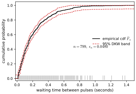
fig_2_1. Download: PDF · SVGTheorem 2.4 (properties of the empirical cdf) p. 14, (2.5)
Let \(X_1,\dots,X_n\sim F\) be independent.
- For each fixed \(x\): \(\E\,\Fn(x)=F(x)\) and \(\V\,\Fn(x)=F(x)(1-F(x))/n\); hence the mean squared error tends to 0 and \(\Fn(x)\convp F(x)\).
- (Glivenko–Cantelli) \(\sup_x|\Fn(x)-F(x)|\convas0\).
- (Dvoretzky–Kiefer–Wolfowitz) For every \(\eps>0\), \[ \Prob\Big(\sup_x|F(x)-\Fn(x)|>\eps\Big)\le2e^{-2n\eps^2}. \tag{2.5} \]
Filling the gap 2.1: proof of Theorem 2.4 (Exercise 2.2) p. 14
Proof
(1) The indicators \(\I(X_i\le x)\) are independent Bernoulli variables with success probability \(F(x)\), so \(n\Fn(x)\sim\mathrm{Binomial}(n,F(x))\): mean \(nF(x)\) and variance \(nF(x)(1-F(x))\). Divide by \(n\) and \(n^2\). Since \(\Fn(x)\) is unbiased, its MSE is its variance, at most \(1/(4n)\to0\), and Chebyshev's inequality gives \(\Prob(|\Fn(x)-F(x)|>\eps)\le1/(4n\eps^2)\to0\).
(3) This is a deep result: Dvoretzky, Kiefer and Wolfowitz (1956) proved it with an unspecified constant \(C\) in front of \(e^{-2n\eps^2}\), and Massart (1990) showed that \(C=2\) works (he proves it when \(e^{-2n\eps^2}\le1/2\); otherwise the right side of (2.5) exceeds 1 and there is nothing to prove). The constant cannot be lowered, because \(\Prob(\sqrt n\sup|\Fn-F|>t)\) tends to Kolmogorov's \(2\sum_{k\ge1}(-1)^{k-1}e^{-2k^2t^2}\sim2e^{-2t^2}\) for continuous \(F\). The companion course proves a DKW-type inequality with an elementary argument and explains the constant: Filling the gap 7.5 there. Here we only need (2.5) as stated.
(2) from (3). Fix \(\eps>0\). By (2.5), \(\sum_n\Prob(\sup_x|\Fn-F|>\eps)\) \(\le\sum_n2e^{-2n\eps^2}\) \(\lt\infty\), so by the first Borel–Cantelli lemma, with probability one \(\sup_x|\Fn-F|>\eps\) happens for only finitely many \(n\). Taking \(\eps=1/k\), \(k=1,2,\dots\), and intersecting the countably many probability-one events gives \(\limsup_n\sup_x|\Fn-F|=0\) almost surely.
(2) without DKW. The VC inequality of Section 2.4 gives the same conclusion with a bound that is proved completely in these notes: by Example 2.45 the half-lines have VC dimension 1, so (2.44) gives \(\Prob(\sup_x|\Fn-F|>\eps)\) \(\le8(n+1)e^{-n\eps^2/32}\), still summable in \(n\), and the Borel–Cantelli argument above applies word for word. (A classical direct proof, which uses only the strong law at finitely many points and the monotonicity of \(F\), is in the companion course: Filling the gap 7.3 there.)
A useful reduction. If \(U_1,\dots,U_n\) are Uniform(0,1) and \(X_i=F^{-1}(U_i)\) with the quantile function \(F^{-1}(u)=\inf\{x:F(x)\ge u\}\), then \(X_i\sim F\), and \(X_i\le x\iff U_i\le F(x)\). Hence \(\Fn(x)=G_n(F(x))\), where \(G_n\) is the empirical cdf of the \(U_i\), and \(\sup_x|\Fn(x)-F(x)|\) \(=\sup_{u\in F(\R)}|G_n(u)-u|\) \(\le\sup_{u}|G_n(u)-u|\), with equality when \(F\) is continuous (then \(F(\R)\supseteq(0,1)\)). So the law of the sup-distance is the same for every continuous \(F\), and is stochastically smaller for discrete \(F\). ∎
p. 15 The DKW inequality turns into a confidence set for the whole function \(F\). Solve \(2e^{-2n\eps^2}=\alpha\) for \(\eps\):
Theorem 2.6 (a nonparametric confidence band) p. 15
Let \(\eps_n=\sqrt{\log(2/\alpha)/(2n)}\), \(L(x)=\max\{\Fn(x)-\eps_n,0\}\) and \(U(x)=\min\{\Fn(x)+\eps_n,1\}\). For every \(F\) and every \(n\),
\[ \Prob\big(L(x)\le F(x)\le U(x)\ \text{for all }x\big)\ge1-\alpha. \]Filling the gap 2.2: from (2.5) to the band, and how conservative it is p. 15
Derivation
If \(\sup_x|\Fn(x)-F(x)|\le\eps_n\) then for every \(x\), \(\Fn(x)-\eps_n\le F(x)\le\Fn(x)+\eps_n\), and since \(0\le F(x)\le1\) also \(L(x)\le F(x)\le U(x)\). So the event of the theorem contains \(\{\sup_x|\Fn-F|\le\eps_n\}\), whose probability is at least \(1-2e^{-2n\eps_n^2}=1-\alpha\) by (2.5). Clipping to \([0,1]\) costs nothing because \(F\) itself lies in \([0,1]\).
How close to \(1-\alpha\)? For continuous \(F\) the coverage is \(\Prob(D_n\le\eps_n)\), where \(D_n=\sup_u|G_n(u)-u|\) for uniforms (Filling the gap 2.1); it does not depend on \(F\) and can be computed exactly. For \(n=100\) and \(\alpha=0.05\) it is 0.9547; as \(n\to\infty\) it tends to \(1-2\sum_{k\ge1}(-1)^{k-1}(\alpha/2)^{k^2}\), which for \(\alpha=0.05\) is \(0.95+2(0.025)^4-\dots\approx0.9500\). The band is therefore essentially exact for continuous data, and conservative for discrete data (where the sup is over fewer points).
Simultaneous against pointwise. At a single \(x\), Theorem 2.4(1) and the CLT give the narrower pointwise interval \(\Fn(x)\pm z_{\alpha/2}\sqrt{\Fn(x)(1-\Fn(x))/n}\), of half-width at most \(z_{\alpha/2}/(2\sqrt n)=0.098\) for \(n=100\), against \(\eps_n=0.136\). But these intervals hold at each \(x\) separately; read together as a band, they miss \(F\) somewhere most of the time. The price of a statement about all \(x\) at once is the factor \(\sqrt{\log(2/\alpha)/2}\big/(z_{\alpha/2}/2)\approx1.39\) at \(\alpha=0.05\).
Example 2.7. p. 15 For the nerve data, \(n=799\) and \(\alpha=0.05\) give \(\eps_n=\sqrt{\log 40/1598}=0.0480\): the dashed lines of Figure 2.1. The book notes that tighter bands exist; the DKW band is used because it is simple and needs no assumption.
2.2 Estimating Statistical Functionals
p. 15 A statistical functional \(T(F)\) is any function of \(F\): the mean \(\mu=\int x\,\d F(x)\), the variance \(\sigma^2=\int(x-\mu)^2\d F(x)\), the median \(F^{-1}(1/2)\), and so on.
See also (companion course): Probability and Statistical Inference, Section 7.2.
Definition 2.8 (plug-in estimator) p. 15, (2.9)
The plug-in estimator of \(\theta=T(F)\) is
\[ \widehat\theta_n=T(\Fn). \tag{2.9} \]A functional of the form \(T(F)=\int a(x)\,\d F(x)\) is linear; its plug-in estimator is the sample average
\[ T(\Fn)=\int a(x)\,\d\Fn(x)=\frac1n\sum_{i=1}^na(X_i). \tag{2.10} \]p. 16 Often \(T(\Fn)\) is approximately Normal,
\[ T(\Fn)\approx\N\big(T(F),\hse^2\big), \tag{2.11} \]for some estimated standard error \(\hse\), and then
\[ T(\Fn)\pm z_{\alpha/2}\,\hse \tag{2.12} \]is an approximate \(1-\alpha\) confidence interval, the Normal-based interval. Section 2.3 gives a general recipe for \(\hse\); Chapter 3 gives two more (jackknife and bootstrap).
Example 2.13 (the mean). p. 16 \(\widehat\mu=\int x\,\d\Fn=\overline X_n\), with \(\se=\sigma/\sqrt n\), estimated by \(\widehat\sigma/\sqrt n\); the interval is \(\overline X_n\pm z_{\alpha/2}\widehat\sigma/\sqrt n\).
Example 2.14 (the variance). pp. 16–17 \(\widehat\sigma^2\) \(=\int x^2\d\Fn-(\int x\,\d\Fn)^2\) \(=n^{-1}\sum_i(X_i-\overline X_n)^2\), which is \((n-1)/n\) times the unbiased \(S_n^2\).
Example 2.15 (the skewness). p. 17 \(\kappa=\E(X-\mu)^3/\sigma^3\) has plug-in estimate \(\widehat\kappa\) \(=n^{-1}\sum_i(X_i-\widehat\mu)^3/\widehat\sigma^3\).
Example 2.16 (correlation). p. 17 With \(Z=(X,Y)\), \(\rho=a(T_1,\dots,T_5)\) where \(T_1,\dots,T_5\) are the linear functionals \(\int x\), \(\int y\), \(\int xy\), \(\int x^2\), \(\int y^2\) (all \(\d F(z)\)) and \(a(t_1,\dots,t_5)\) \(=(t_3-t_1t_2)/\sqrt{(t_4-t_1^2)(t_5-t_2^2)}\). Plugging in gives the sample correlation
\[ \widehat\rho=\frac{\sum_i(X_i-\overline X_n)(Y_i-\overline Y_n)}{\sqrt{\sum_i(X_i-\overline X_n)^2}\sqrt{\sum_i(Y_i-\overline Y_n)^2}}. \]Example 2.17 (quantiles). p. 17 For \(F\) strictly increasing with density \(f\), \(T(F)=F^{-1}(p)\) is the \(p\)th quantile. Since \(\Fn\) is a step function, define \(\Fn^{-1}(p)=\inf\{x:\Fn(x)\ge p\}\), the \(p\)th sample quantile: it is the order statistic \(X_{(\lceil np\rceil)}\). (For \(n=26\) and \(p=1/2\) it is \(X_{(13)}\), not the average of \(X_{(13)}\) and \(X_{(14)}\) that most software reports; this matters in Exercise 2.13.)
Filling the gap 2.3: what the plug-in examples rely on pp. 16–17
Details
Linear functionals. By (2.10), \(T(\Fn)\) is an average of the independent variables \(a(X_i)\), so it is unbiased for \(T(F)\), consistent by the law of large numbers whenever \(\E|a(X)|\lt\infty\), and \(\sqrt n(T(\Fn)-T(F))\convd\N(0,\V a(X))\) by the CLT whenever \(\E a(X)^2\lt\infty\). This is (2.11) with \(\hse^2\) \(=n^{-1}\cdot n^{-1}\sum_i(a(X_i)-T(\Fn))^2\).
The variance. \(\E\widehat\sigma^2=\frac{n-1}n\sigma^2\): write \(\sum(X_i-\overline X)^2\) \(=\sum(X_i-\mu)^2-n(\overline X-\mu)^2\) and take expectations, \(n\sigma^2-\sigma^2\). The bias \(-\sigma^2/n\) is of smaller order than the standard error, which is of order \(n^{-1/2}\); this is why "in practice there is little difference" between \(\widehat\sigma^2\) and \(S_n^2\).
Smooth functions of averages. The variance, skewness and correlation are \(a(T_1(F),\dots,T_m(F))\) with linear \(T_j\) and smooth \(a\). Their plug-in estimates are \(a\) of a vector of sample averages, so the multivariate delta method gives asymptotic normality with variance \(\nabla a^\top\Sigma\nabla a/n\), \(\Sigma\) the covariance of \((a_1(X),\dots,a_m(X))\). Section 2.3 reaches the same answer through the chain rule (2.33) for influence functions.
Sample quantiles. The definition \(\Fn^{-1}(p)=\inf\{x:\Fn(x)\ge p\}\) makes the "switching relation" exact: for every \(x\), \(\Fn^{-1}(p)\le x\iff\Fn(x)\ge p\). (\(\Leftarrow\) is the definition of the infimum; \(\Rightarrow\) holds because \(\Fn\) is right-continuous and non-decreasing, so the infimum is attained.) Since \(\Fn(x)\ge p\) means at least \(\lceil np\rceil\) observations are \(\le x\), the sample quantile is the order statistic \(X_{(\lceil np\rceil)}\). The switching relation is what turns statements about \(\Fn\) into statements about quantiles: Filling the gap 2.8 uses it for asymptotic normality.
The Glivenko–Cantelli theorem says \(\Fn\to F\) uniformly; it suggests that \(T(\Fn)\to T(F)\) whenever \(T\) is continuous for the sup-norm (Exercise 2.5), and that \(T(\Fn)\) is asymptotically Normal when \(T\) is suitably differentiable. That is the subject of the next section.
2.3 Influence Functions
p. 18 The influence function measures how a functional responds to a small amount of contamination at one point. It plays the role for plug-in estimators that the score function plays for maximum likelihood: its variance is the asymptotic variance.
See also (companion course): Probability and Statistical Inference, the influence function and the nonparametric delta method.
Definition 2.18 (Gateaux derivative and influence function) p. 18, (2.19)–(2.21)
The Gateaux derivative of \(T\) at \(F\) in the direction of the distribution \(G\) is
\[ L_F(G)=\lim_{\eps\to0}\frac{T\big((1-\eps)F+\eps G\big)-T(F)}{\eps}. \tag{2.19} \]For \(G=\delta_x\) write \(L_F(x)\equiv L_F(\delta_x)\), the influence function:
\[ L_F(x)=\lim_{\eps\to0}\frac{T\big((1-\eps)F+\eps\delta_x\big)-T(F)}{\eps}. \tag{2.20} \]The empirical influence function is \(\widehat L(x)=L_{\Fn}(x)\):
\[ \widehat L(x)=\lim_{\eps\to0}\frac{T\big((1-\eps)\Fn+\eps\delta_x\big)-T(\Fn)}{\eps}. \tag{2.21} \](Only \(\eps\downarrow0\) makes sense, since \((1-\eps)F+\eps G\) must be a distribution.)
Theorem 2.22 (linear functionals) p. 18, (2.23)–(2.26)
Let \(T(F)=\int a(x)\,\d F(x)\). Then:
- \(L_F(x)=a(x)-T(F)\) and \(\widehat L(x)=a(x)-T(\Fn)\).
- For every distribution \(G\), \[ T(G)=T(F)+\int L_F(x)\,\d G(x). \tag{2.23} \]
- \(\int L_F(x)\,\d F(x)=0\).
- Let \(\tau^2\) \(=\int L_F^2(x)\,\d F(x)\) \(=\int(a(x)-T(F))^2\d F(x)\). If \(\tau^2\lt\infty\), \[ \sqrt n\big(T(F)-T(\Fn)\big)\convd\N(0,\tau^2). \tag{2.24} \]
- Let \[ \widehat\tau^2=\frac1n\sum_{i=1}^n\widehat L^2(X_i)=\frac1n\sum_{i=1}^n\big(a(X_i)-T(\Fn)\big)^2. \tag{2.25} \] Then \(\widehat\tau^2\convp\tau^2\) and \(\hse/\se\convp1\), where \(\hse=\widehat\tau/\sqrt n\) and \(\se=\sqrt{\V(T(\Fn))}\).
- \[ \frac{\sqrt n\big(T(F)-T(\Fn)\big)}{\widehat\tau}\convd\N(0,1). \tag{2.26} \]
Filling the gap 2.4: the complete proof of Theorem 2.22 (Exercise 2.1) pp. 18–19
Proof
(1) A linear functional is affine along mixtures: \(T((1-\eps)F+\eps\delta_x)\) \(=(1-\eps)\int a\,\d F+\eps\int a\,\d\delta_x\) \(=(1-\eps)T(F)+\eps a(x)\). The difference quotient in (2.20) is therefore \(a(x)-T(F)\) for every \(\eps\in(0,1]\), and so is the limit. The same computation with \(\Fn\) in place of \(F\) gives \(\widehat L\).
(2) \(\int L_F\,\d G\) \(=\int a\,\d G-T(F)\int\d G\) \(=T(G)-T(F)\), because \(G\) has total mass 1. (Here \(a\) must be \(G\)-integrable.)
(3) Take \(G=F\) in (2): \(\int L_F\,\d F=T(F)-T(F)=0\).
(4) Take \(G=\Fn\) in (2): \(T(\Fn)-T(F)\) \(=\int L_F\,\d\Fn\) \(=n^{-1}\sum_iL_F(X_i)\). The \(L_F(X_i)\) are independent, identically distributed, with mean 0 by (3) and variance \(\tau^2\lt\infty\), so the CLT gives \(\sqrt n(T(\Fn)-T(F))\convd\N(0,\tau^2)\). The book writes \(T(F)-T(\Fn)\); since \(\N(0,\tau^2)\) is symmetric, the two statements are the same.
(5) Write \(b_i=a(X_i)-T(F)=L_F(X_i)\) and \(\bar b=n^{-1}\sum b_i=T(\Fn)-T(F)\). Then \(a(X_i)-T(\Fn)=b_i-\bar b\), so
\[ \widehat\tau^2=\frac1n\sum_i(b_i-\bar b)^2=\frac1n\sum_ib_i^2-\bar b^2. \]By the strong law, \(n^{-1}\sum b_i^2\to\E b_1^2=\tau^2\) and \(\bar b\to\E b_1=0\) almost surely, hence \(\widehat\tau^2\to\tau^2\) almost surely, and in probability. Because \(T(\Fn)\) is an average, its exact variance is \(\se^2=\tau^2/n\), so \(\hse/\se=\widehat\tau/\tau\convp1\) when \(\tau>0\) (continuous mapping, \(t\mapsto\sqrt t\)).
(6) \(\sqrt n(T(F)-T(\Fn))\convd\N(0,\tau^2)\) and \(\tau/\widehat\tau\convp1\); by Slutsky's theorem the product converges to \(\N(0,\tau^2)/\tau=\N(0,1)\). ∎
The analogy with the score. For a smooth parametric model \(f(x;\theta)\), the score \(s_\theta(x)=\partial_\theta\log f(x;\theta)\) has \(\int s_\theta f\,\d x=0\), and the MLE satisfies \(\widehat\theta-\theta\approx I(\theta)^{-1}n^{-1}\sum s_\theta(X_i)\). For a plug-in estimator, \(T(\Fn)-T(F)\approx n^{-1}\sum L_F(X_i)\) with \(\int L_F\,\d F=0\): the influence function is the "standardised score" of the nonparametric problem, and \(\V(T(\Fn))\approx\int L_F^2\,\d F/n\).
p. 19 For a nonlinear \(T\), (2.23) no longer holds exactly, but it may hold up to a small remainder, and then the same conclusions follow.
Theorem 2.27 (Hadamard differentiable functionals) pp. 19–20, (2.28)–(2.30)
If \(T\) is Hadamard differentiable at \(F\) with respect to \(d(F,G)=\sup_x|F(x)-G(x)|\) (Section 2.6), then
\[ \sqrt n\big(T(\Fn)-T(F)\big)\convd\N(0,\tau^2), \tag{2.28} \]where \(\tau^2=\int L_F(x)^2\d F(x)\). Also
\[ \frac{T(\Fn)-T(F)}{\hse}\convd\N(0,1), \tag{2.29} \]where \(\hse=\widehat\tau/\sqrt n\) and
\[ \widehat\tau^2=\frac1n\sum_{i=1}^n\widehat L^2(X_i). \tag{2.30} \]The book prints (2.30) as "\(\widehat\tau=\dots\)"; the left side must be \(\widehat\tau^2\), as in (2.25) and (2.31). See Notes on the text.
The nonparametric delta method p. 20, (2.31)
A \(1-\alpha\), pointwise asymptotic confidence interval for \(T(F)\) is
\[ T(\Fn)\pm z_{\alpha/2}\,\hse,\qquad \hse=\frac{\widehat\tau}{\sqrt n},\qquad\widehat\tau^2=\frac1n\sum_{i=1}^n\widehat L^2(X_i). \tag{2.31} \]"Pointwise" because it is a statement about one functional at a time, as opposed to the simultaneous band of Theorem 2.6.
Filling the gap 2.5: why Hadamard differentiability gives (2.28), and what (2.29) needs in addition pp. 19–20, 23–24
Proof
Setting. Let \(\ell^\infty(\R)\) be the bounded functions on \(\R\) with the sup norm, \(\cF\subset\ell^\infty(\R)\) the cdfs. Following Section 2.6, \(T\) is Hadamard differentiable at \(F\) (tangentially to a set \(\cD_0\)) if there is a continuous linear map \(L_F:\ell^\infty(\R)\to\R\) such that
\[ \frac{T(F+t_nD_n)-T(F)}{t_n}\to L_F(D)\quad\text{whenever }t_n\downarrow0,\ \|D_n-D\|_\infty\to0,\ D\in\cD_0,\ F+t_nD_n\in\cF. \]Its value at \(D=\delta_x-F\) is the influence function: \((1-\eps)F+\eps\delta_x=F+\eps(\delta_x-F)\), so taking \(D_n\equiv\delta_x-F\) gives \(L_F(x)=L_F(\delta_x-F)\).
Step 1 (Donsker's theorem). The empirical process \(\mathbb G_n=\sqrt n(\Fn-F)\) converges in distribution in \(\ell^\infty(\R)\) to \(\mathbb G=B\circ F\), where \(B\) is a Brownian bridge on \([0,1]\) (Donsker, 1952; van der Vaart, 1998, Theorem 19.3). Its paths lie in \(\cD_0=\{h\circ F\}\), with \(h\) continuous on \([0,1]\) and \(h(0)=h(1)=0\), and we take Hadamard differentiability tangentially to this set.
Step 2 (the key step). Define \(g_n(h)=\sqrt n\{T(F+h/\sqrt n)-T(F)\}\). Hadamard differentiability with \(t_n=1/\sqrt n\) says exactly: if \(h_n\to h\in\cD_0\) then \(g_n(h_n)\to L_F(h)\). Now \(\sqrt n(T(\Fn)-T(F))=g_n(\mathbb G_n)\). By the almost sure representation theorem (Dudley; van der Vaart, 1998, Theorem 18.9) there are versions \(\tilde{\mathbb G}_n\) and \(\tilde{\mathbb G}\) with the same laws as \(\mathbb G_n\) and \(\mathbb G\) such that \(\tilde{\mathbb G}_n\to\tilde{\mathbb G}\) uniformly, almost surely. Applying the deterministic statement path by path gives \(g_n(\tilde{\mathbb G}_n)\) \(\to L_F(\tilde{\mathbb G})\) almost surely, hence \(g_n(\mathbb G_n)\convd L_F(\mathbb G)\). (Equivalently: the extended continuous mapping theorem, van der Vaart, 1998, Theorem 18.11.)
Step 3 (the limit is \(\N(0,\tau^2)\)). \(L_F\) is continuous and linear, so \(L_F(\mathbb G_n)\convd L_F(\mathbb G)\) by the continuous mapping theorem. By linearity, \(L_F(\mathbb G_n)\) \(=\sqrt n\,L_F(\Fn-F)\) \(=n^{-1/2}\sum_iL_F(\delta_{X_i}-F)\) \(=n^{-1/2}\sum_iL_F(X_i)\), a normalised sum of i.i.d. variables. Assume \(\tau^2=\E L_F(X)^2\lt\infty\). If \(m=\E L_F(X)\) were nonzero, \(n^{-1/2}\sum_iL_F(X_i)=\sqrt n\,m+O_P(1)\) would diverge, contradicting convergence in distribution; so \(m=0\), the CLT gives the limit \(\N(0,\tau^2)\), and the two limits agree: \(L_F(\mathbb G)\sim\N(0,\tau^2)\). This proves (2.28), and shows that \(T(\Fn)=T(F)\) \({}+n^{-1}\sum_iL_F(X_i)\) \({}+o_P(n^{-1/2})\): the nonlinear functional behaves like the linear one of Theorem 2.22.
Why Hadamard and not Gateaux. The direction in which we perturb \(F\) is the random, \(n\)-dependent function \(\mathbb G_n\). Gateaux differentiability controls the remainder only along each fixed direction, so it says nothing about \(g_n(\mathbb G_n)\). Hadamard differentiability asks for the remainder to vanish along converging sequences of directions, which is uniformity over compact sets; that is exactly what Step 2 uses. (Fréchet differentiability, uniformity over bounded sets, would also work but fails for quantiles.)
What (2.29) needs. (2.29) follows from (2.28) by Slutsky once \(\widehat\tau^2\convp\tau^2\). For linear \(T\) this is Theorem 2.22(5). In general it is an extra condition: it holds when \(\widehat L=L_{\Fn}\) is close to \(L_F\) in mean square, e.g. for smooth functions of means (\(\widehat L\) is a continuous function of sample moments, so the law of large numbers applies) and for quantiles with a consistent density estimate in (2.36). It does not follow from Hadamard differentiability alone, so (2.29) should be read with this proviso.
Which functionals qualify. The \(p\)-quantile is Hadamard differentiable tangentially to \(\cD_0\) at any \(F\) that is differentiable at \(\theta=F^{-1}(p)\) with \(f(\theta)>0\) (van der Vaart, 1998, Lemma 21.3), with \(L_F(D)=-D(\theta)/f(\theta)\). Smooth functions of finitely many sample means are covered when the underlying \(a_j\) are bounded. But the mean itself is not Hadamard (not even continuously) dependent on \(F\) in the sup norm when the support is unbounded: \(F_\eps=(1-\eps)F+\eps\delta_{1/\eps^2}\) has \(\|F_\eps-F\|_\infty\le\eps\) while its mean is \((1-\eps)\mu+1/\eps\to\infty\). Theorem 2.27 therefore does not cover Example 2.32; Theorem 2.22 does, needing only a finite variance. ∎
Example 2.32 (the mean). p. 20 \(T((1-\eps)F+\eps\delta_x)=(1-\eps)\theta+\eps x\), so \(L(x)=x-\theta\), \(\widehat L(x)=x-\overline X_n\) and \(\hse^2=\widehat\sigma^2/n\) with \(\widehat\sigma^2\) \(=n^{-1}\sum(X_i-\overline X_n)^2\); a 95% interval is \(\overline X_n\pm2\,\hse\).
p. 20 If \(T(F)=a(T_1(F),\dots,T_m(F))\) for a differentiable \(a\), the chain rule gives
\[ L(x)=\sum_{i=1}^m\frac{\partial a}{\partial t_i}L_i(x),\qquad L_i(x)=\lim_{\eps\to0}\frac{T_i((1-\eps)F+\eps\delta_x)-T_i(F)}{\eps}. \tag{2.33} \]Filling the gap 2.6: the chain rule (2.33), and the influence functions of the variance and the skewness p. 20
Derivation
Chain rule. Put \(\phi(\eps)=(T_1(F_\eps),\dots,T_m(F_\eps))\) with \(F_\eps=(1-\eps)F+\eps\delta_x\). If each \(T_i(F_\eps)\) is differentiable from the right at \(\eps=0\) with derivative \(L_i(x)\) and \(a\) is differentiable at \(\phi(0)\), then \(\eps\mapsto a(\phi(\eps))\) is right-differentiable at 0 with derivative \(\nabla a(\phi(0))^\top\phi'(0)\) \(=\sum_i\partial_ia\,L_i(x)\): the ordinary chain rule for a function of one real variable.
Central moments. Let \(\mu_\eps\) be the mean of \(F_\eps\): \(\mu_\eps=\mu+\eps(x-\mu)\). The \(k\)th central moment is \(m_k(\eps)\) \(=(1-\eps)\E(X-\mu_\eps)^k+\eps(x-\mu_\eps)^k\). Differentiating at \(\eps=0\) (with \(\mu_0'=x-\mu\) and \(m_1=0\)):
\[ m_k'(0)=-m_k+(x-\mu)^k-k\,m_{k-1}(x-\mu). \]For \(k=2\): \(L_{\sigma^2}(x)=(x-\mu)^2-\sigma^2\). For \(k=3\): \(L_{m_3}(x)=(x-\mu)^3-m_3-3\sigma^2(x-\mu)\).
Skewness. \(\kappa=m_3/(\sigma^2)^{3/2}\), so by the chain rule
\[ L_\kappa(x)=\frac{(x-\mu)^3-m_3-3\sigma^2(x-\mu)}{\sigma^3}-\frac32\,\kappa\,\frac{(x-\mu)^2-\sigma^2}{\sigma^2}. \]At \(F=\N(0,1)\) this is \(x^3-3x\), the third Hermite polynomial, with \(\tau^2=\E(X^3-3X)^2=6\): the familiar \(\V(\widehat\kappa)\approx6/n\) for Normal data. The cubic growth of \(L_\kappa\) means that \(\tau^2\) involves the sixth moment, and that \(\widehat\tau^2\) is a very noisy estimate of it; Figure 2.S3 shows the consequence. The book's formula for \(\widehat\kappa\) uses exactly these plug-in moments, and the closed forms above were confirmed numerically against difference quotients of the weighted plug-in.
Example 2.34 (correlation). pp. 20–21 With \(T_1,\dots,T_5\) and \(a\) as in Example 2.16, (2.33) gives
\[ L(x,y)=\tilde x\,\tilde y-\tfrac12T(F)\big(\tilde x^2+\tilde y^2\big),\qquad \tilde x=\frac{x-\int x\,\d F}{\sqrt{\int x^2\d F-(\int x\,\d F)^2}},\quad \tilde y=\frac{y-\int y\,\d F}{\sqrt{\int y^2\d F-(\int y\,\d F)^2}}. \]Filling the gap 2.7: the correlation influence function (Exercise 2.9) p. 21
Derivation
Write \(\mu_x,\mu_y,\sigma_x^2,\sigma_y^2,\sigma_{xy}\) for the moments of \(F\), \(\rho=\sigma_{xy}/(\sigma_x\sigma_y)\), and \(a=(t_3-t_1t_2)(v_xv_y)^{-1/2}\) with \(v_x=t_4-t_1^2\), \(v_y=t_5-t_2^2\). The influence functions of the linear pieces are \(L_1=x-\mu_x\), \(L_2=y-\mu_y\), \(L_3=xy-\E XY\), \(L_4=x^2-\E X^2\), \(L_5=y^2-\E Y^2\) (Theorem 2.22(1)). The partial derivatives at \(T(F)\) are
\[ \partial_1a=-\frac{\mu_y}{\sigma_x\sigma_y}+\rho\frac{\mu_x}{\sigma_x^2},\quad \partial_2a=-\frac{\mu_x}{\sigma_x\sigma_y}+\rho\frac{\mu_y}{\sigma_y^2},\quad \partial_3a=\frac1{\sigma_x\sigma_y},\quad \partial_4a=-\frac{\rho}{2\sigma_x^2},\quad \partial_5a=-\frac{\rho}{2\sigma_y^2}. \]Group the terms. Those with \(\sigma_x\sigma_y\) in the denominator give \(\{xy-\E XY-\mu_y(x-\mu_x)\) \({}-\mu_x(y-\mu_y)\}/(\sigma_x\sigma_y)\) \(=\{(x-\mu_x)(y-\mu_y)-\sigma_{xy}\}/(\sigma_x\sigma_y)\) \(=\tilde x\tilde y-\rho\). Those with \(\sigma_x^2\) give \(\rho\{\mu_x(x-\mu_x)-\tfrac12(x^2-\E X^2)\}/\sigma_x^2\); since \(\E X^2=\sigma_x^2+\mu_x^2\), the brace equals \(-\tfrac12(x-\mu_x)^2+\tfrac12\sigma_x^2\), so this group is \(-\tfrac\rho2(\tilde x^2-1)\). Likewise for \(y\). Adding,
\[ L(x,y)=\tilde x\tilde y-\rho-\tfrac\rho2(\tilde x^2-1)-\tfrac\rho2(\tilde y^2-1)=\tilde x\tilde y-\tfrac\rho2(\tilde x^2+\tilde y^2), \]which is the book's formula. For a bivariate Normal, \(\tau^2=\E L^2=(1-\rho^2)^2\) (expand with \(\E\tilde x^4=3\), \(\E\tilde x^2\tilde y^2=1+2\rho^2\), \(\E\tilde x^3\tilde y=3\rho\)), the classical asymptotic variance of \(\sqrt n(\widehat\rho-\rho)\). ∎
Example 2.35 (quantiles). p. 21, (2.36) Let \(F\) be strictly increasing with positive density \(f\) and \(\theta=T(F)=F^{-1}(p)\). Then
\[ L(x)=\begin{cases}\dfrac{p-1}{f(\theta)}, & x\le\theta,\\[2mm] \dfrac{p}{f(\theta)}, & x>\theta,\end{cases} \]and the asymptotic variance of \(T(\Fn)\) is
\[ \tau_n^2=\frac1n\int L^2(x)\,\d F(x)=\frac{p(1-p)}{nf^2(\theta)}. \tag{2.36} \]To use (2.36) we must estimate \(f(\theta)\); Chapter 3 shows that the bootstrap avoids this.
Filling the gap 2.8: the quantile influence function (Exercise 2.10) and a direct proof of asymptotic normality p. 21
Derivation
The influence function. Assume \(f\) is continuous and positive near \(\theta\). Let \(F_\eps(y)=(1-\eps)F(y)+\eps\I(y\ge x)\) and \(\theta_\eps=F_\eps^{-1}(p)\). Case \(x>\theta\). For small \(\eps\), \(\theta_\eps\lt x\), so \(\theta_\eps\) solves \((1-\eps)F(\theta_\eps)=p\), i.e. \(\theta_\eps=F^{-1}(p/(1-\eps))\). By the inverse function theorem \(\frac{\d}{\d\eps}\theta_\eps|_0\) \(=\frac{p}{f(\theta)}\). Case \(x\lt\theta\). For small \(\eps\), \(\theta_\eps>x\) and \((1-\eps)F(\theta_\eps)+\eps=p\), so \(\theta_\eps=F^{-1}((p-\eps)/(1-\eps))\), with derivative \(\frac{p-1}{f(\theta)}\) at 0. (This is the book's hint: differentiate \(p=F_\eps(T(F_\eps))\) implicitly, \(0=-F(\theta)+f(\theta)\theta'+\I(\theta\ge x)\).) At \(x=\theta\) the quantile does not move (\(\theta_\eps=\theta\) for all small \(\eps\)), so \(L(\theta)=0\) rather than \((p-1)/f(\theta)\); a single point has probability zero under \(F\) and changes nothing below.
(2.36). \(\int L^2\d F\) \(=\frac{(p-1)^2}{f^2}F(\theta)+\frac{p^2}{f^2}(1-F(\theta))\) \(=\frac{(1-p)^2p+p^2(1-p)}{f^2}\) \(=\frac{p(1-p)}{f^2(\theta)}\). For the median of \(\N(0,1)\) this is \(\pi/2\): the sample median needs about \(\pi/2\approx1.57\) times as many Normal observations as the mean for the same precision.
Asymptotic normality directly. Let \(\widehat\theta=\Fn^{-1}(p)\), fix \(t\in\R\) and put \(x_n=\theta+t/\sqrt n\), \(p_n=F(x_n)\). By the switching relation (Filling the gap 2.3), \(\{\sqrt n(\widehat\theta-\theta)\) \(\le t\}\) \(=\{\Fn(x_n)\) \(\ge p\}\), and \(n\Fn(x_n)\sim\mathrm{Binomial}(n,p_n)\). Then
\[ \Prob\big(\sqrt n(\widehat\theta-\theta)\le t\big)=\Prob\Big(\frac{\sqrt n(\Fn(x_n)-p_n)}{\sqrt{p_n(1-p_n)}}\ge\frac{\sqrt n(p-p_n)}{\sqrt{p_n(1-p_n)}}\Big). \]By differentiability, \(\sqrt n(p_n-p)\) \(=\sqrt n(F(\theta+t/\sqrt n)-F(\theta))\) \(\to tf(\theta)\), and \(p_n\to p\). The standardised binomial on the left converges to \(\N(0,1)\) by the Lindeberg CLT for triangular arrays (bounded summands, variance \(p_n(1-p_n)\to p(1-p)>0\)), and uniformly in the threshold by Pólya's theorem, since the limit is continuous. So the probability tends to \(1-\Phi\big(-tf(\theta)/\sqrt{p(1-p)}\big)\) \(=\Phi\big(tf(\theta)/\sqrt{p(1-p)}\big)\): \(\sqrt n(\widehat\theta-\theta)\) \(\convd\N(0,p(1-p)/f^2(\theta))\), in agreement with (2.36). (The companion course gives the same argument in its Filling the gap 7.11.) ∎
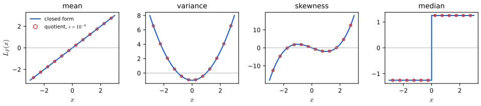
fig_2_s1. Download: PDF · SVG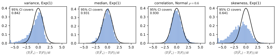
fig_2_s3. Download: PDF · SVG2.4 Empirical Probability Distributions
p. 21 The book marks this section as optional; it generalises the DKW inequality from half-lines to arbitrary classes of sets. Let \(X_1,\dots,X_n\) be independent with law \(P\) (on \(\R\) or \(\R^d\)) and define the empirical probability distribution
\[ \Pn(A)=\frac{\#\{i:X_i\in A\}}{n}. \tag{2.37} \]For one fixed set \(A\), \(n\Pn(A)\sim\mathrm{Binomial}(n,P(A))\), and Hoeffding's inequality (bounded summands in \([0,1]\)) gives
\[ \Prob\big(|\Pn(A)-P(A)|>\eps\big)\le2e^{-2n\eps^2}. \tag{2.38} \]See also (companion courses): Hoeffding's inequality in Probability and Statistical Inference, Theorem 4.5; the VC dimension in Statistical Learning: Theory and Methods, Section 7.9.
We want the same kind of statement for \(\sup_{A\in\cA}|\Pn(A)-P(A)|\) over a whole class \(\cA\). DKW is the case \(\cA=\{(-\infty,t]:t\in\R\}\), but it is special to one dimension. A union bound over infinitely many sets is useless; the way out is that, on \(n\) points, an infinite class acts only through the finitely many subsets it can cut out. For a finite set \(R=\{x_1,\dots,x_n\}\) let
\[ N_\cA(R)=\#\big\{R\cap A:\ A\in\cA\big\} \tag{2.39} \]be the number of subsets of \(R\) picked out by \(\cA\). \(R\) is shattered by \(\cA\) if \(N_\cA(R)=2^n\). The shatter coefficient is
\[ s(\cA,n)=\max_{R\in F_n}N_\cA(R), \tag{2.40} \]where \(F_n\) is the collection of all sets of \(n\) points.
Theorem 2.41 (Vapnik and Chervonenkis, 1971) p. 22, (2.42)
For any \(P\), \(n\) and \(\eps>0\),
\[ \Prob\Big(\sup_{A\in\cA}|\Pn(A)-P(A)|>\eps\Big)\le8\,s(\cA,n)\,e^{-n\eps^2/32}. \tag{2.42} \]Filling the gap 2.9: a complete proof of the Vapnik–Chervonenkis inequality p. 22
Proof
We assume the suprema below are measurable (true when a countable subclass gives the same supremum, as for all the classes in this chapter). The argument has three steps: replace \(P\) by a second sample, replace the difference of the two samples by random signs, and then condition on the data, where only finitely many sets matter. The proof follows Devroye, Györfi and Lugosi (1996, Theorem 12.5).
Step 0. If \(n\eps^2\lt2\), the right side is at least \(8e^{-1/16}>1\) and there is nothing to prove. Assume \(n\eps^2\ge2\).
Step 1 (symmetrisation by a ghost sample). Let \(X_1',\dots,X_n'\) be an independent copy of the sample, with empirical measure \(\Pn'\). We show
\[ \Prob\Big(\sup_A|\Pn(A)-P(A)|>\eps\Big)\le2\,\Prob\Big(\sup_A|\Pn(A)-\Pn'(A)|>\tfrac\eps2\Big). \]On the event \(E=\{\sup_A|\Pn(A)-P(A)|>\eps\}\) choose a set \(A^*\) (depending on \(X_1,\dots,X_n\) only) with \(|\Pn(A^*)-P(A^*)|>\eps\). Conditionally on \(X_1,\dots,X_n\), \(\Pn'(A^*)\) is a binomial proportion with variance at most \(1/(4n)\), so by Chebyshev
\[ \Prob\big(|\Pn'(A^*)-P(A^*)|\le\tfrac\eps2\,\big|\,X_1,\dots,X_n\big)\ge1-\frac{1/(4n)}{\eps^2/4}=1-\frac1{n\eps^2}\ge\frac12. \]When both \(|\Pn(A^*)-P(A^*)|>\eps\) and \(|\Pn'(A^*)-P(A^*)|\le\eps/2\) hold, the triangle inequality gives \(|\Pn(A^*)-\Pn'(A^*)|>\eps/2\). Hence \(\Prob(\sup_A|\Pn-\Pn'|>\eps/2)\) \(\ge\E\big[\I_E\cdot\tfrac12\big]\) \(=\tfrac12\Prob(E)\).
Step 2 (random signs). Let \(\sigma_1,\dots,\sigma_n\) be independent signs, \(\pm1\) with probability \(\tfrac12\), independent of both samples. Swapping \(X_i\) and \(X_i'\) does not change the joint law of the two samples, and it changes the sign of \(\I_A(X_i)-\I_A(X_i')\) for every \(A\) at once. So the process \(\big(\sum_i(\I_A(X_i)-\I_A(X_i'))\big)_{A}\) has the same law as \(\big(\sum_i\sigma_i(\I_A(X_i)-\I_A(X_i'))\big)_{A}\), and
\[ \Prob\Big(\sup_A|\Pn(A)-\Pn'(A)|>\tfrac\eps2\Big)=\Prob\Big(\sup_A\Big|\frac1n\sum_i\sigma_i\big(\I_A(X_i)-\I_A(X_i')\big)\Big|>\tfrac\eps2\Big)\le2\,\Prob\Big(\sup_A\Big|\frac1n\sum_i\sigma_i\I_A(X_i)\Big|>\tfrac\eps4\Big), \]where the last step splits the sum by the triangle inequality (if the difference exceeds \(\eps/2\), one of the two parts exceeds \(\eps/4\)) and uses that the two parts have the same law.
Step 3 (condition on the data; union bound; Hoeffding). Fix \(X_1=x_1,\dots,X_n=x_n\). The vector \((\I_A(x_1),\dots,\I_A(x_n))\) depends on \(A\) only through \(A\cap\{x_1,\dots,x_n\}\), so as \(A\) ranges over \(\cA\) it takes at most \(N_\cA(\{x_1,\dots,x_n\})\le s(\cA,n)\) values (if some \(x_i\) coincide there are fewer distinct points, and \(s(\cA,\cdot)\) is non-decreasing). For each such value, \(\sum_i\sigma_i\I_A(x_i)\) is a sum of independent, mean-zero terms with values in \([-1,1]\), and Hoeffding's inequality gives
\[ \Prob\Big(\Big|\sum_i\sigma_i\I_A(x_i)\Big|>\frac{n\eps}4\Big)\le2\exp\Big(-\frac{2(n\eps/4)^2}{n\cdot2^2}\Big)=2e^{-n\eps^2/32}. \]A union bound over the at most \(s(\cA,n)\) distinct vectors bounds the conditional probability by \(2s(\cA,n)e^{-n\eps^2/32}\), and integrating over the data keeps the bound. Collecting the factors \(2\cdot2\cdot2\) of the three steps gives (2.42). ∎
Remarks. The constants 8 and 32 come from this crude argument; sharper versions exist (e.g. with \(s(\cA,2n)\) and exponent \(n\eps^2/8\)), and for half-lines the DKW inequality is far better (Example 2.45). The proof never uses the dimension of the space: only the combinatorics of \(\cA\) on finite sets enter.
p. 22 Theorem 2.41 is useful only if \(s(\cA,n)\) grows slower than \(e^{n\eps^2/32}\). If \(s(\cA,n)=2^n\) for all \(n\), set \(\VC(\cA)=\infty\); otherwise the Vapnik–Chervonenkis dimension \(\VC(\cA)\) is the largest \(k\) with \(s(\cA,k)=2^k\), i.e. the size of the largest set shattered by \(\cA\).
Theorem 2.43 (polynomial growth) p. 22, (2.44)
If \(\cA\) has finite VC dimension \(v\), then \(s(\cA,n)\le n^v+1\), and therefore
\[ \Prob\Big(\sup_{A\in\cA}|\Pn(A)-P(A)|>\eps\Big)\le8(n^v+1)e^{-n\eps^2/32}. \tag{2.44} \]Filling the gap 2.10: Sauer's lemma, and the bound \(n^v+1\) p. 22
Proof
Sauer's lemma (Sauer, 1972; Vapnik and Chervonenkis, 1971): if \(\VC(\cA)=v\) then \(s(\cA,n)\le\Phi_v(n):=\sum_{i=0}^v\binom ni\).
Fix \(R\) with \(|R|=n\) and let \(\mathcal C=\{R\cap A:A\in\cA\}\), a family of subsets of \(R\). We prove the stronger statement (Pajor's lemma): \(|\mathcal C|\) is at most the number of subsets of \(R\) shattered by \(\mathcal C\). Since \(\mathcal C\) shatters only sets that \(\cA\) shatters, all of size at most \(v\), and there are \(\Phi_v(n)\) subsets of \(R\) of size at most \(v\), Sauer's lemma follows.
Induction on \(n\). For \(n=0\), \(\mathcal C\) is \(\emptyset\) or \(\{\emptyset\}\), and in the second case \(\emptyset\) is shattered: the claim holds. For \(n\ge1\) pick \(x\in R\), let \(R'=R\setminus\{x\}\) and define two families on \(R'\):
\[ \mathcal C_0=\{B\subseteq R':B\in\mathcal C\ \text{or}\ B\cup\{x\}\in\mathcal C\},\qquad \mathcal C_1=\{B\subseteq R':B\in\mathcal C\ \text{and}\ B\cup\{x\}\in\mathcal C\}. \]Each \(B\in\mathcal C_0\) accounts for one or two members of \(\mathcal C\), two exactly when \(B\in\mathcal C_1\); so \(|\mathcal C|=|\mathcal C_0|+|\mathcal C_1|\). By induction \(|\mathcal C_j|\) \(\le\#\{S\subseteq R':S\text{ shattered by }\mathcal C_j\}\). If \(S\subseteq R'\) is shattered by \(\mathcal C_0\), it is shattered by \(\mathcal C\) (each trace on \(S\) is realised by \(B\) or \(B\cup\{x\}\), which have the same trace on \(S\)). If \(S\) is shattered by \(\mathcal C_1\), then \(S\cup\{x\}\) is shattered by \(\mathcal C\) (each trace on \(S\) comes with both choices at \(x\)). The sets of the first kind do not contain \(x\) and those of the second kind do, so they are different, and \(\mathcal C\) shatters at least \(|\mathcal C_0|+|\mathcal C_1|=|\mathcal C|\) sets. Maximising over \(R\) gives the lemma.
From \(\Phi_v(n)\) to \(n^v+1\). We show \(\Phi_v(n)\le n^v+1\) for all \(n\ge0\), \(v\ge0\) (with \(0^0=1\)). For \(v=0\): \(1\le2\). For \(v=1\): \(1+n=n^1+1\). For \(n\le1\): \(\Phi_v(n)\le2\le n^v+1\) when \(n=1\), and \(=1\) when \(n=0\). For \(v\ge2\), \(n\ge2\), induct on \(v\): \(\Phi_v(n)\) \(=\Phi_{v-1}(n)+\binom nv\) \(\le n^{v-1}+1+\binom nv\), and
\[ \binom nv\le\frac{n(n-1)\,n^{v-2}}{v!}\le\frac{n^{v-1}(n-1)}2\le n^{v-1}(n-1)=n^v-n^{v-1}, \]so \(\Phi_v(n)\le n^v+1\). (Checked numerically for all \(n\lt300\), \(v\lt25\).) Inserting into (2.42) gives (2.44). ∎
Consequence. With finite VC dimension the right side of (2.44) is summable in \(n\) for every \(\eps>0\), so \(\sup_{A\in\cA}|\Pn(A)-P(A)|\to0\) almost surely (Borel–Cantelli, as in Filling the gap 2.1): a uniform law of large numbers over \(\cA\), the Glivenko–Cantelli property. Solving \(8(n^v+1)e^{-n\eps^2/32}=\alpha\) gives the half-width \(\eps_n=\sqrt{32\log(8(n^v+1)/\alpha)/n}\), of order \(\sqrt{v\log n/n}\).
Example 2.45. p. 22 \(\cA=\{(-\infty,x]:x\in\R\}\) shatters every one-point set but no two-point set, so \(\VC(\cA)=1\). Since \(P((-\infty,x])=F(x)\) and \(\Pn((-\infty,x])=\Fn(x)\), (2.44) gives \(\Prob(\sup_x|\Fn(x)-F(x)|>\eps)\) \(\le8(n+1)e^{-n\eps^2/32}\), which is much looser than DKW: for the nerve data (\(n=799\), \(\alpha=0.05\)) the corresponding band has half-width 0.686, against 0.048 (Figure 2.S4, right). The VC bound is not the tightest possible; its value is its generality.
Example 2.46. p. 23 Closed intervals shatter any two points but no three: with \(x\lt y\lt z\), an interval containing \(x\) and \(z\) contains \(y\). So \(\VC=2\).
Example 2.47. p. 23 Half-planes in \(\R^2\) shatter any three points not on a line, but no four points, so \(\VC=3\); in \(\R^d\), half-spaces have VC dimension \(d+1\).
Example 2.48. p. 23 Axis-parallel rectangles shatter some four-point sets (a "diamond") but no five-point set, so \(\VC=4\).
Filling the gap 2.11: proofs for Examples 2.45 to 2.48, and how the demonstration counts picked-out sets pp. 22–23
Proofs
Half-lines. \(\{x\}\) is shattered: \((-\infty,x-1]\) picks \(\emptyset\), \((-\infty,x]\) picks \(\{x\}\). For \(x\lt y\), any \((-\infty,t]\ni y\) has \(t\ge y>x\), so \(\{y\}\) alone is never picked out. On \(n\) points half-lines pick exactly the \(n+1\) "initial segments" of the sorted points: \(s(\cA,n)=n+1=\Phi_1(n)\).
Intervals. For \(x\lt y\), the four subsets come from an empty interval, \([x,x]\), \([y,y]\) and \([x,y]\). For \(x\lt y\lt z\), an interval is convex, so it contains \(y\) if it contains \(x\) and \(z\). Intervals pick out exactly the runs of consecutive sorted points: \(1+n+\binom n2=\Phi_2(n)\) subsets.
Half-planes. Three points \(a,b,c\) not on a line: \(\emptyset\) and \(\{a,b,c\}\) are trivial; a single vertex is separated from the line through the other two by a parallel line between them, which also picks the complementary pair. No four points \(a,b,c,d\) are shattered. Either (i) three are on a line, say \(b\) between \(a\) and \(c\): a half-plane is convex, so it cannot contain \(a,c\) without \(b\); or (ii) one point, say \(d\), lies in the triangle \(abc\): a half-plane containing \(a,b,c\) contains their convex hull and so \(d\); or (iii) the four are in convex position, labelled around the hull, so the diagonals \(ac\) and \(bd\) cross at a point \(o\). If a half-plane \(H\) picked out \(\{a,c\}\), then \(o\in[a,c]\subset H\) while \(b,d\) lie in the complement, an open half-plane, which is convex and so contains \(o\in[b,d]\): a contradiction. These cases are exhaustive.
Rectangles. A diamond is shattered. Take four points, each strictly extreme in one of the four directions (highest, lowest, leftmost, rightmost), such as \((0,1),(-1,0),(1,0),(0,-1)\). For a subset \(S\), the smallest rectangle containing \(S\) (its bounding box) excludes every other point, since that point is strictly beyond all of \(S\) in its own direction. No five points are shattered. Among five points choose a leftmost, a rightmost, a highest and a lowest one (at most four points). At least one point \(z\) remains, and it lies in the bounding box of the chosen ones. Any rectangle containing all points but \(z\) contains that bounding box, hence \(z\). So \(\VC=4\). In general a set \(S\) is picked out by a rectangle if and only if its bounding box contains no other point, which is how the code and the demonstration count.
Counting for half-planes and discs. The code and the demonstration enumerate picked-out sets exactly, for points in general position (no three on a line, no four on a circle). Half-planes: if a closed half-plane picks out \(S\ne\emptyset,R\), translate its boundary line until it touches a point, then rotate it about that point until it touches a second one, never letting a point cross the line. The final line passes through two points \(x_i,x_j\), and \(S\) is the set of points strictly on one side plus a subset of \(\{x_i,x_j\}\). Conversely every such combination is picked out by a small perturbation of the line. Discs: shrink a disc that picks out \(S\) about its centre until a point of \(S\) is on its boundary, then shrink it towards that point (internally tangent discs, which only lose points) until a second point is on the boundary; then move the centre along the bisector of the two boundary points until a third point of \(R\) reaches the circle, in whichever direction this happens first. So \(S\) is the interior of a circle through one point (radius 0), two points (as a diameter, if no third point is met) or three points, plus some of the points on that circle, and conversely each of these combinations is realised by a perturbed circle (three non-collinear points: the map from (centre, radius) to the three signed powers is locally onto). The enumeration agrees with a linear-programming test of every subset on random point sets (for discs via the lifting \((x,y)\mapsto(x,y,x^2+y^2)\), under which discs become lower half-spaces).
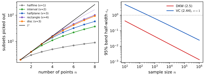
fig_2_s4. Download: PDF · SVG2.5 Bibliographic Remarks
p. 23 The book points to Serfling (1980), Davison and Hinkley (1997), Shao and Tu (1995), Fernholz (1983) and van der Vaart (1998) for statistical functionals, and to Devroye, Györfi and Lugosi (1996), van der Vaart (1998) and van der Vaart and Wellner (1996) for VC theory. The proofs in Filling the gap 2.5 follow van der Vaart (1998, Chapters 18 to 21), and those in 2.9 and 2.10 follow Devroye, Györfi and Lugosi (1996, Chapters 12 and 13).
2.6 Appendix
pp. 23–24 Let \(\cF\) be the set of all distribution functions and \(\cD\) the linear space they span. Writing \(T((1-\eps)F+\eps G)=T(F+\eps D)\) with \(D=G-F\in\cD\), the Gateaux derivative \(L_F(D)\) is defined by
\[ \lim_{\eps\downarrow0}\Big|\frac{T(F+\eps D)-T(F)}{\eps}-L_F(D)\Big|=0, \]so that \(T(F+\eps D)-T(F)=\eps L_F(D)+o(\eps)\) along each fixed direction \(D\). Equip \(\cD\) with a metric \(d\). \(T\) is Hadamard differentiable at \(F\) if there is a linear functional \(L_F\) on \(\cD\) such that for every \(\eps_n\to0\) and \(D,D_1,D_2,\dots\in\cD\) with \(d(D_n,D)\to0\) and \(F+\eps_nD_n\in\cF\),
\[ \lim_{n\to\infty}\Big|\frac{T(F+\eps_nD_n)-T(F)}{\eps_n}-L_F(D_n)\Big|=0. \]When \(L_F\) is continuous (as it must be in the theory), \(L_F(D_n)\) may be replaced by \(L_F(D)\), which is the form used in Filling the gap 2.5; that box explains why this uniformity over converging directions is exactly what the proof of Theorem 2.27 needs, and which functionals have it.
Notes on the text
Points where the printed text needs care (the book's website has no errata list; the evidence is given in each case).
Page 20, (2.30): \(\widehat\tau\) should be \(\widehat\tau^2\)
(2.30) reads \(\widehat\tau=n^{-1}\sum_i\widehat L^2(X_i)\). The right side is a mean of squares, an estimate of \(\tau^2=\int L_F^2\,\d F\), and \(\hse=\widehat\tau/\sqrt n\) only gives the right scale if \(\widehat\tau^2\) equals it; (2.25) and the box (2.31) both have \(\widehat\tau^2\). For the mean of the Old Faithful waiting times, \(n^{-1}\sum\widehat L^2=184.1\), whose square root 13.57 over \(\sqrt{272}\) is the correct \(\hse=0.823\).
Theorem 2.27 and (2.29): consistency of \(\widehat\tau\) is an extra assumption
Hadamard differentiability gives (2.28), but (2.29) also needs \(\widehat\tau^2\convp\tau^2\), which the theorem asserts without a condition. It holds in the book's examples (smooth functions of means; quantiles with a consistent density estimate) but not for every Hadamard differentiable \(T\). Also, the mean of Example 2.32 is not Hadamard differentiable for the sup norm when the support is unbounded (it is not even continuous), so it is covered by Theorem 2.22, not by Theorem 2.27 (Filling the gap 2.5).
Page 23, Section 2.6: a missing \(-T(F)\)
The appendix writes \(T(F+\eps D)\approx\eps L_F(D)+o(\eps)\); the left side should be \(T(F+\eps D)-T(F)\), as the preceding display defining \(L_F(D)\) shows.
Example 2.35: the value at \(x=\theta\)
The displayed influence function gives \((p-1)/f(\theta)\) at \(x=\theta\), but contamination exactly at the quantile does not move it, so the derivative there is 0 (Filling the gap 2.8). This changes nothing in (2.36), since \(\{\theta\}\) has probability zero.
Exercises 2.4 and 2.13
Exercise 2.4 is printed with a garbled symbol; from context (and the matching exercise in the author's earlier book) it asks for the limiting distribution of \(\sqrt{\Fn(x)}\). The address given in Exercise 2.13 for the cloud seeding data no longer works; the data are clouds.dat on the book's website.
2.7 Exercises
All 15 exercises of Chapter 2 (pp. 24–25), restated in my own words, with complete solutions (hidden). Numerical answers come from the chapter's code (exercise_numbers) on the book's data.
Exercise 2.1. Give the details of the proof of Theorem 2.22.
Solution
See Filling the gap 2.4: each of the six claims is proved there in full, together with the remark on the sign convention in (2.24) and (2.26).
Exercise 2.2. Prove Theorem 2.4.
Solution
See Filling the gap 2.1: part 1 from the binomial law of \(n\Fn(x)\); part 2 from part 3 (or from the VC inequality, proved in Filling the gap 2.9) by the Borel–Cantelli lemma; part 3 is Massart's form of the DKW inequality, with a complete elementary DKW-type proof in the companion course.
Exercise 2.3 (computer experiment). Draw 100 observations from \(\N(0,1)\), compute the 95% band for \(F\), repeat 1000 times and record how often the band contains the true \(F\). Repeat with Cauchy data.
Solution
With independent Normal and Cauchy samples (numpy generator, seeds 23 and 24) the band contained \(F\) in 949 and 958 of the 1000 repetitions. Both are consistent with the exact coverage 0.9547 (Monte Carlo standard error \(\sqrt{0.95\cdot0.05/1000}=0.007\)). The point of the exercise is that heavy tails do not matter: by the reduction in Filling the gap 2.1, \(\sup_x|\Fn-F|\) has the same law for every continuous \(F\). If both populations are generated from the same uniforms, \(X_i=F^{-1}(U_i)\), the band covers in exactly the same repetitions: the demonstration does this and finds 944 of 1000 for both. (Containment is checked exactly: \(\sup_x|\Fn-F|\) is the largest of the numbers \(i/n-F(X_{(i)})\) and \(F(X_{(i)})-(i-1)/n\) for continuous \(F\).)
Exercise 2.4. For fixed \(x\), find the limiting distribution of \(\sqrt{\Fn(x)}\).
Solution
Let \(F=F(x)\). If \(0\lt F\lt1\), the CLT gives \(\sqrt n(\Fn(x)-F)\convd\N(0,F(1-F))\), and the delta method with \(g(t)=\sqrt t\), \(g'(F)=1/(2\sqrt F)\), gives
\[ \sqrt n\big(\sqrt{\Fn(x)}-\sqrt{F}\big)\convd\N\Big(0,\frac{F(1-F)}{4F}\Big)=\N\Big(0,\frac{1-F}4\Big). \]The variance-stabilising transformation for a proportion is \(\arcsin\sqrt t\) (limit variance \(1/4\) whatever \(F\)); \(\sqrt t\) only removes the factor \(F\). If \(F=0\) or \(F=1\), \(\Fn(x)=F\) almost surely and the limit is degenerate. (With \(n=400\), \(F=0.3\): simulated \(n\V\sqrt{\Fn}=0.175\), against \(0.7/4=0.175\).)
Exercise 2.5. Suppose \(|T(F)-T(G)|\le C\|F-G\|_\infty\) for some \(0\lt C\lt\infty\) (2.49). Show that \(T(\Fn)\to T(F)\) almost surely, and that the mean satisfies (2.49) when \(|X|\le M\).
Solution
\(|T(\Fn)-T(F)|\) \(\le C\sup_x|\Fn(x)-F(x)|\) \(\to0\) almost surely by Glivenko–Cantelli: Lipschitz continuity in the sup norm transfers uniform consistency of \(\Fn\) to \(T(\Fn)\).
For distributions on \([-M,M]\), integration by parts (or Fubini) gives \(\int x\,\d F(x)\) \(=\int_0^M(1-F(x))\d x-\int_{-M}^0F(x)\d x\) \(=M-\int_{-M}^MF(x)\,\d x\). Hence
\[ \Big|\int x\,\d F-\int x\,\d G\Big|=\Big|\int_{-M}^M(G(x)-F(x))\,\d x\Big|\le2M\|F-G\|_\infty, \]so (2.49) holds with \(C=2M\) on the class of distributions supported in \([-M,M]\), which contains \(\Fn\). Without bounded support the mean is not continuous in the sup norm at all (Filling the gap 2.5).
Exercise 2.6. For distinct points \(x\) and \(y\), find \(\Cov(\Fn(x),\Fn(y))\).
Solution
\(\Cov(\Fn(x),\Fn(y))\) \(=n^{-2}\sum_{i,j}\Cov(\I(X_i\) \(\le x),\I(X_j\) \(\le y))\); terms with \(i\ne j\) vanish by independence, and for \(i=j\), \(\E[\I(X\le x)\I(X\le y)]=F(\min(x,y))\). So
\[ \Cov\big(\Fn(x),\Fn(y)\big)=\frac{F(\min(x,y))-F(x)F(y)}{n}=\frac{F(x\wedge y)\,(1-F(x\vee y))}{n}, \]which is positive: the empirical cdf is high (or low) over whole stretches at once. Up to the factor \(1/n\) this is the covariance of the Brownian bridge \(B(F(x))\), the limit in Donsker's theorem (Filling the gap 2.5).
Exercise 2.7. Let \(X_1,\dots,X_n\sim\) Bernoulli\((p)\) and, independently, \(Y_1,\dots,Y_m\sim\) Bernoulli\((q)\). Find the plug-in estimator, estimated standard error and an approximate 90% interval for \(p\), and then for \(p-q\).
Solution
\(p=\int x\,\d F\) is linear, so \(\widehat p=\overline X_n\), \(\widehat L(x)=x-\widehat p\) and \(\widehat\tau^2\) \(=n^{-1}\sum(X_i-\widehat p)^2\) \(=\widehat p(1-\widehat p)\) (since \(X_i^2=X_i\)). Thus \(\hse(\widehat p)\) \(=\sqrt{\widehat p(1-\widehat p)/n}\) and a 90% interval is \(\widehat p\pm1.645\,\hse\). For \(\theta=p-q\), \(\widehat\theta=\overline X_n-\overline Y_m\); the two samples are independent, so variances add: \(\hse(\widehat\theta)\) \(=\sqrt{\widehat p(1-\widehat p)/n+\widehat q(1-\widehat q)/m}\), and the interval is \(\widehat\theta\pm1.645\,\hse(\widehat\theta)\). (The approximation needs \(np\), \(n(1-p)\), \(mq\), \(m(1-q)\) not too small.)
Exercise 2.8. For fixed \(a\lt b\), let \(\theta=T(F)=F(b)-F(a)\) and \(\widehat\theta=\Fn(b)-\Fn(a)\). Find the influence function, the estimated standard error and an approximate \(1-\alpha\) interval.
Solution
\(\theta=\int\I(a\lt x\le b)\,\d F(x)\) is linear with \(a(x)=\I(a\lt x\le b)\), so by Theorem 2.22, \(L(x)=\I(a\lt x\le b)-\theta\) and \(\widehat L(x)=\I(a\lt x\le b)-\widehat\theta\). Then \(\widehat\tau^2\) \(=n^{-1}\sum_i(\I(a\) \(\lt X_i\) \(\le b)-\widehat\theta)^2\) \(=\widehat\theta(1-\widehat\theta)\), \(\hse=\sqrt{\widehat\theta(1-\widehat\theta)/n}\), and the interval is \(\widehat\theta\pm z_{\alpha/2}\hse\). (Exact alternative: \(n\widehat\theta\) is binomial. Simultaneous alternative, valid for all \(a,b\) at once: \([\max(L(b)-U(a),0),\ U(b)-L(a)]\) from the DKW band, wider.) For the nerve data, \(\widehat F(0.6)-\widehat F(0.4)=0.0926\) with \(\hse=0.0103\) and 95% interval \((0.0725,0.1127)\).
Exercise 2.9. Verify the influence function of Example 2.34.
Solution
See Filling the gap 2.7, which also gives \(\tau^2=(1-\rho^2)^2\) for Normal data.
Exercise 2.10. Verify the influence function of Example 2.35, by differentiating \(p=F_\eps(T(F_\eps))\) with respect to \(\eps\) at \(\eps=0\), where \(F_\eps=(1-\eps)F+\eps\delta_x\).
Solution
See Filling the gap 2.8 (including the value at \(x=\theta\) and a direct proof of the asymptotic normality of the sample quantile).
Exercise 2.11. For the magnitudes of the earthquakes near Fiji (book website), estimate \(F\), plot a 95% confidence envelope, and find an approximate 95% interval for \(F(4.9)-F(4.3)\).
Solution
\(n=1000\), so the DKW half-width is \(\eps_n=\sqrt{\log40/2000}=0.0429\); Figure 2.S2 shows \(\Fn\) and the band. \(\Fn(4.9)=0.802\) and \(\Fn(4.3)=0.276\), so \(\widehat\theta=0.526\); by Exercise 2.8, \(\hse=\sqrt{0.526\cdot0.474/1000}=0.0158\) and the 95% interval is \((0.495,\,0.557)\). About half of these earthquakes have magnitudes in \((4.3,4.9]\).
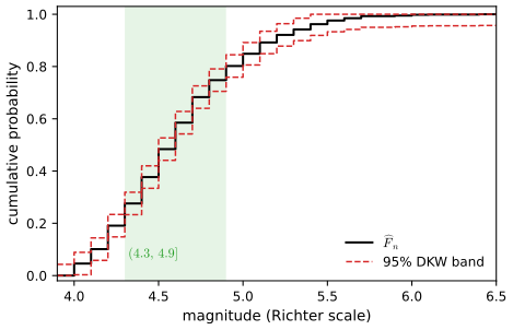
Figure 2.S2 (supplementary). Exercise 2.11: the empirical cdf of the Fiji earthquake magnitudes (recorded to one decimal, hence the large steps) with the 95% DKW band (\(\eps_n=0.0429\)); the shaded interval is \((4.3,4.9]\). Not a figure of the book. Code: ch02_estimating_cdf_functionals.py, fig_2_s2. Download: PDF · SVG▶ DemoExercise 2.11 interactivelyMove \(a\) and \(b\), change \(\alpha\), compare with pointwise intervals.Exercise 2.12. For the Old Faithful waiting times (book website), estimate the mean waiting time with a standard error and a 90% interval; then estimate the median waiting time.
Solution
\(n=272\). \(\overline X=70.90\) minutes and \(\widehat\sigma=13.57\) (plug-in, divisor \(n\)), so \(\hse=13.57/\sqrt{272}=0.823\) and the 90% interval is \(70.90\pm1.645\cdot0.823=(69.54,\,72.25)\). The sample median \(\Fn^{-1}(1/2)=X_{(136)}\) is 76 minutes. The mean lies well below the median because the waiting times are bimodal (short waits after short eruptions), which also makes the median's standard error depend on the density at 76 minutes, a peak of the distribution: (2.36) with a kernel estimate gives \(\hse=0.97\) (demonstration), and Chapter 3 gives the bootstrap answer.
Exercise 2.13. In a 1975 experiment, 26 of 52 clouds, chosen at random, were seeded with silver nitrate. Let \(\theta\) be the difference between the median rainfall of seeded and unseeded clouds. Estimate \(\theta\), its standard error using (2.36) with some estimate of the density, and give a 95% interval.
Solution
Estimate. With the book's sample quantile \(X_{(13)}\): seeded median 200.7, unseeded median 41.1 acre-feet, so \(\widehat\theta=159.6\). (With the more common average of \(X_{(13)}\) and \(X_{(14)}\): \(221.6-44.2=177.4\).)
Standard error. The groups are independent, so \(\hse(\widehat\theta)^2=\hse_1^2+\hse_2^2\), each from (2.36) with \(p=1/2\): \(\hse_j\) \(=1/(2\sqrt{26}\,\widehat f_j(\widehat m_j))\). The density at the median must be estimated:
- Kernel estimate on the raw scale (Gaussian kernel, bandwidth \(0.9\min(s,\mathrm{IQR}/1.34)n^{-1/5}\)): \(\widehat f=0.00168\) (seeded) and \(0.00501\) (unseeded), \(\hse_j=58.3\) and \(19.6\), \(\hse(\widehat\theta)=61.5\), interval \(159.6\pm1.96\cdot61.5=(39.0,\,280.2)\).
- Kernel estimate on the log scale. Rainfall is extremely skewed (from 1 to 2746), so one bandwidth cannot suit the dense low values and the sparse high ones. On the log scale the data are roughly symmetric; the median commutes with the monotone map \(\log\), and the change of variables gives \(f(m)=g(\log m)/m\), with \(g\) the density of \(\log X\). This gives \(\widehat f=0.00154\) and \(0.00615\), \(\hse(\widehat\theta)=65.8\), interval \((30.6,\,288.6)\).
- The bootstrap (Chapter 3), no density needed: 4000 resamples of each group give \(\hse=63.9\).
The three standard errors agree to within about 7%, and all intervals exclude 0: seeding raised the median rainfall. A symmetric Normal interval is crude here (the sampling distribution of a difference of medians from 26 skewed observations is itself skewed); an interval for the ratio of medians on the log scale would be more natural for these data.
Exercise 2.14. Let \(\cA\) be the set of discs \(\{(x,y):(x-a)^2+(y-b)^2\le c^2\}\) in the plane. Find \(\VC(\cA)\).
Solution
\(\VC(\cA)=3\).
Three points are shattered. Take \(a,b,c\) not on a line. \(\emptyset\) and singletons: tiny discs. All three: a large disc. A pair, say \(\{a,b\}\): by Example 2.47 a closed half-plane \(H=\{z:u\cdot z\le t\}\) contains \(a,b\) with \(u\cdot a,u\cdot b\lt t\) and has \(u\cdot c>t\). The discs \(D_R\) with centre \(z_0-Ru\) and radius \(R\), where \(z_0\) is a point on the line \(u\cdot z=t\), increase to the open half-plane \(\{u\cdot z\lt t\}\) as \(R\to\infty\) and never contain \(c\); for \(R\) large they contain \(a\) and \(b\).
No four points are shattered. As for half-planes there are three cases. (i) Three on a line: a disc is convex, so it cannot take the two outer points without the middle one. (ii) One point inside the triangle of the others: a disc containing the three contains their convex hull. (iii) Convex position \(a,b,c,d\) (in order around the hull), diagonals crossing at \(o\). Suppose discs \(D_1\) and \(D_2\) pick out \(\{a,c\}\) and \(\{b,d\}\). Write \(D_j=\{z:\pi_j(z)\le0\}\) with \(\pi_j(z)=|z-m_j|^2-r_j^2\). Then \(\pi_1\le0\lt\pi_2\) at \(a\) and \(c\), and \(\pi_2\le0\lt\pi_1\) at \(b\) and \(d\), so \(h=\pi_1-\pi_2\) is negative at \(a,c\) and positive at \(b,d\). But \(|z|^2\) cancels in \(h\), which is therefore affine (the "radical axis" of the two circles is \(h=0\)): the open half-planes \(\{h\lt0\}\ni a,c\) and \(\{h>0\}\ni b,d\) are convex and disjoint, yet both contain \(o\). Contradiction. So at least one of the two diagonal pairs is lost, and four points give at most 15 subsets (the demonstration shows 15 for a kite, where only one diagonal pair is lost).
Sauer's lemma then gives \(s(\cA,n)\le1+n+\binom n2+\binom n3\), and this is attained by points in general position (Figure 2.S4: 93 for \(n=8\)). Equivalently, the lifting \((x,y)\mapsto(x,y,x^2+y^2)\) turns discs into the lower half-spaces of \(\R^3\) restricted to a paraboloid.
Exercise 2.15. The empirical cdf as a nonparametric maximum likelihood estimator: for data on \([0,1]\), divide the interval into bins of width \(\Delta\), find the MLE among distributions with constant density on each bin, and show that its cdf converges to \(\Fn\) as \(\Delta\to0\).
Solution
Let \(m=1/\Delta\) be an integer, \(B_j=((j-1)\Delta,j\Delta]\) (with 0 put in \(B_1\)) and \(N_j=\#\{i:X_i\in B_j\}\). A density constant on the bins is \(f=\sum_j(\theta_j/\Delta)\I_{B_j}\) with \(\theta_j\ge0\), \(\sum_j\theta_j=1\). The log-likelihood is \(\sum_jN_j\log\theta_j-n\log\Delta\). By Gibbs' inequality (\(\sum_j\widehat\theta_j\log(\theta_j/\widehat\theta_j)\) \(\le\log\sum_j\theta_j\) \(=0\) by Jensen, with \(\widehat\theta_j=N_j/n\)), it is maximised by \(\widehat\theta_j=N_j/n\): the histogram. Its cdf at \(x\in B_k\) is
\[ \widehat F_\Delta(x)=\sum_{j\lt k}\frac{N_j}n+\frac{N_k}n\cdot\frac{x-(k-1)\Delta}{\Delta},\qquad\text{while}\qquad\Fn(x)=\sum_{j\lt k}\frac{N_j}n+\frac{\#\{i:X_i\in B_k,\ X_i\le x\}}n. \]So \(|\widehat F_\Delta(x)-\Fn(x)|\le N_k/n\), the mass of the bin containing \(x\). If \(x\) is not one of the data points, then for \(\Delta\lt\min_i|x-X_i|\) the bin containing \(x\) holds no observation, \(N_k=0\), and \(\widehat F_\Delta(x)=\Fn(x)\) exactly. Hence \(\widehat F_\Delta\to\Fn\) at every point except the \(n\) observations, i.e. at every continuity point of \(\Fn\): convergence in distribution. The convergence is not uniform: \(\widehat F_\Delta\) is continuous and \(\Fn\) jumps by at least \(1/n\) at each \(X_i\), so \(\sup_x|\widehat F_\Delta-\Fn|\ge1/(2n)\) for every \(\Delta\). In this sense \(\Fn\) is the limit of maximum likelihood estimators over ever richer models: the "nonparametric MLE".
Demonstrations for this chapter
Each demonstration runs in the browser on the book's data, with seeded random numbers, and links back to these notes. The ▶ Demo boxes above open them already set to the case under discussion; the numbers they show are those of the Python code.
| Demonstration | What you can see | Sections and results |
|---|---|---|
| Confidence bands for a cdf: DKW against VC | The nerve, Fiji and Old Faithful data with the DKW band, the VC band and pointwise intervals; an interval for \(F(b)-F(a)\); coverage of the band for Normal, Cauchy and Exponential samples. Presets: 1 Figure 2.1; 2 Exercise 2.11; 3 Exercise 2.3, Normal; 4 Cauchy; 5 Example 2.45. | 2.1, 2.4; Theorem 2.6, Exercises 2.3, 2.8, 2.11 |
| Influence functions and the delta method | The empirical influence function of the mean, variance, skewness, quantiles and correlation over the data; the difference quotient (2.21) as \(\eps\to0\); standard errors and intervals (2.31). Presets: 1 mean; 2 variance; 3 median; 4 correlation; 5 skewness. | 2.3; Theorems 2.22, 2.27, Filling the gaps 2.6–2.8 |
| Shattering and the VC dimension | Click points into the plane; every subset is shown as a tile, green if half-lines, intervals, half-planes, rectangles or discs pick it out; Sauer's bound; a search over random point sets. Presets: 1 half-lines; 2 intervals; 3 half-planes; 4 rectangles; 5 discs. | 2.4; Theorem 2.43, Filling the gap 2.11, Exercise 2.14 |
Related demonstrations in the companion course Probability and Statistical Inference: the DKW band, Glivenko–Cantelli and the delta method. The Python code for every figure of this page is code/ch02_estimating_cdf_functionals.py (see the code index).
References
- Cox, D. R. and Lewis, P. A. W. (1966). The Statistical Analysis of Series of Events. Methuen, London.
- Davison, A. C. and Hinkley, D. V. (1997). Bootstrap Methods and Their Application. Cambridge University Press.
- Devroye, L., Györfi, L. and Lugosi, G. (1996). A Probabilistic Theory of Pattern Recognition. Springer, New York.
- Donsker, M. D. (1952). Justification and extension of Doob's heuristic approach to the Kolmogorov–Smirnov theorems. Annals of Mathematical Statistics, 23, 277–281.
- Dvoretzky, A., Kiefer, J. and Wolfowitz, J. (1956). Asymptotic minimax character of the sample distribution function and of the classical multinomial estimator. Annals of Mathematical Statistics, 27, 642–669.
- Fernholz, L. T. (1983). von Mises Calculus for Statistical Functionals. Lecture Notes in Statistics 19, Springer, New York.
- Hampel, F. R. (1974). The influence curve and its role in robust estimation. Journal of the American Statistical Association, 69, 383–393.
- Massart, P. (1990). The tight constant in the Dvoretzky–Kiefer–Wolfowitz inequality. Annals of Probability, 18, 1269–1283.
- Pajor, A. (1985). Sous-espaces \(\ell_1^n\) des espaces de Banach. Hermann, Paris.
- Sauer, N. (1972). On the density of families of sets. Journal of Combinatorial Theory, Series A, 13, 145–147.
- Serfling, R. J. (1980). Approximation Theorems of Mathematical Statistics. Wiley, New York.
- Shao, J. and Tu, D. (1995). The Jackknife and Bootstrap. Springer, New York.
- Simpson, J., Olsen, A. and Eden, J. C. (1975). A Bayesian analysis of a multiplicative treatment effect in weather modification. Technometrics, 17, 161–166.
- van der Vaart, A. W. (1998). Asymptotic Statistics. Cambridge University Press.
- van der Vaart, A. W. and Wellner, J. A. (1996). Weak Convergence and Empirical Processes. Springer, New York.
- Vapnik, V. N. and Chervonenkis, A. Ya. (1971). On the uniform convergence of relative frequencies of events to their probabilities. Theory of Probability and Its Applications, 16, 264–280.
- Wasserman, L. (2004). All of Statistics: A Concise Course in Statistical Inference. Springer, New York.
- Wasserman, L. (2006). All of Nonparametric Statistics. Springer, New York. Chapter 2, pp. 13–25. www.stat.cmu.edu/~larry/all-of-nonpar.
The numerical statements in the text (the band half-widths and coverage, the influence functions against difference quotients, the asymptotic variances, the exercise answers and the counts of picked-out subsets) were confirmed numerically.