Normal Means and Minimax Theory
Observe \(Z_i=\theta_i+\sn\epsilon_i\) for \(i=1,\dots,n\), with as many unknown means as observations. This innocent-looking model is the common core of nonparametric regression, density estimation and the white noise model: expand the unknown function in an orthonormal basis and its coefficients become many Normal means. The chapter asks how well the means can be estimated in the worst case (Pinsker's theorem and the minimax rate \(n^{-2m/(2m+1)}\) over Sobolev ellipsoids), which estimators achieve this without knowing the smoothness (James–Stein, blockwise James–Stein), how to estimate the risk of an estimator from the data (Stein's unbiased risk estimate), how small a confidence ball can be (no smaller than order \(\sn n^{1/4}\)), and why thresholding comes within a factor \(2\log n\) of an oracle for sparse vectors.
Ch. 1 Introduction Ch. 2 The cdf and functionals Ch. 3 Bootstrap and jackknife Ch. 4 Smoothing Ch. 5 Regression Ch. 6 Density estimation Ch. 7 Normal means and minimax Ch. 8 Orthogonal functions Ch. 9 Wavelets Ch. 10 Other topics
How to read these notes
They follow the book. Sections carry the book's numbers (7.1, 7.2, ...) and every displayed equation that appears in the book carries the book's own equation number, e.g. \((7.19)\), so you can read these notes next to the book. Equations without a number are steps that the book skips.
Filling the gaps. This chapter states many results without proof or quotes them from the literature, and its appendix proofs skip steps. Each Filling the gap box gives a complete argument: assumptions stated, every step justified. Where a result is a deep theorem of the research literature (Theorems 7.50, 7.82 and 7.85, and the lower bound in (7.91)), the box gives a precise statement, the idea of the proof and the reference. Proofs start hidden: open one with its bar, or use the button below.
Figures and demonstrations. Figure 7.2 and Table 7.1 are reproduced from scratch by the Python code; Figure 7.1 is a schematic and is described in words. Eight supplementary figures (numbered 7.S1–7.S8) illustrate results the book states without a picture. The ▶ Demo boxes open an interactive demonstration already set to the case being discussed.
Main reference
L. Wasserman, All of Nonparametric Statistics, Springer (2006), Chapter 7, pages 145–182 (book website, with the data sets: www.stat.cmu.edu/~larry/all-of-nonpar). Section, equation, figure and exercise numbers below refer to this book. Further reading is listed in the references; the standard monograph on this material is Johnstone's Gaussian Estimation: Sequence and Wavelet Models, which the book cites as Johnstone (2003).
The explanations, derivations, figures and code are my own; equations are cited by their numbers in the book.
Companion courses
This chapter is the advanced sequel to material in two companion courses on this site:
- Probability and Statistical Inference (Wasserman 2004, same author and notation), Chapter 12: risk, Bayes and minimax rules (Section 12.4, with "a Bayes rule with constant risk is minimax", Theorem 12.11), the minimax risk \(\sigma^2c^2/(\sigma^2+c^2)\) of many Normal means over a ball (Filling the gap 12.13), and Stein's paradox (Section 12.7): Stein's lemma (Lemma 12.C), the James–Stein estimator dominates the MLE for \(k\ge3\) (Theorem 12.D), and James–Stein as empirical Bayes (Filling the gap 12.19). Chapter 21: orthonormal bases, Parseval's identity and the cosine basis (Section 21.1), orthogonal series regression (Section 21.3).
- Statistical Learning: Theory and Methods: ridge regression and the lasso as penalised least squares (Section 3.4), \(C_p\), AIC and BIC (Sections 7.5 and 7.7), the effective number of parameters, which is the divergence term of SURE (Section 7.6).
- Demonstrations of the same ideas: Stein's paradox and mean squared error of shrinkage (Probability and Statistical Inference).
Where those notes prove a result completely (Stein's lemma, the domination of the MLE for \(k\ge3\), the minimax value over a ball by a Bayes argument), these notes give the statement, a short argument and the link. New here: SURE for general covariance and for thresholding, the exact risk of James–Stein, Pinsker's theorems for ellipsoids with the constant, the minimax rate over Sobolev classes, adaptive blockwise estimation, the three confidence balls and the lower bounds on their size, and the oracle inequality for thresholding.
The chapter at a glance
- 7.1–7.3 The model \(Z_i=\theta_i+\sn\epsilon_i\); orthonormal bases, Parseval, Sobolev spaces and ellipsoids (Theorem 7.11); regression becomes a Normal means problem with \(\sn^2=\sigma^2/n\) (Figure 7.S1).
- 7.4 SURE: \(\E\sure(Z)=R(\hth,\theta)\) for any weakly differentiable estimator (Theorem 7.17); the formulas for linear shrinkage and soft thresholding (Figure 7.S2).
- 7.5 Minimax risk: \(\sigma^2c^2/(\sigma^2+c^2)\) over a ball (Theorem 7.28); rate \(n^{-2m/(2m+1)}\) and Pinsker's constant over Sobolev ellipsoids (Theorems 7.32 and 7.36); linear estimators are asymptotically minimax.
- 7.6 James–Stein loses at most \(2\sn^2\) to the best linear shrinkage, for every \(\theta\) (Theorem 7.47), and is asymptotically minimax over balls without knowing the radius (Theorem 7.48).
- 7.7 Blockwise James–Stein is adaptively minimax over all Sobolev ellipsoids (Theorem 7.50).
- 7.8–7.10 Confidence balls: the \(\chi^2\) ball, pre-testing, Baraud's ball (Theorem 7.59), the pivotal ball (Figure 7.2, Table 7.1); no honest ball can have radius below order \(\sn n^{1/4}\) (Theorem 7.74), and bands cannot adapt at all.
- 7.11 Ridge, soft and hard thresholding as penalised least squares (Theorem 7.88); soft thresholding at \(\sn\sqrt{2\log n}\) is within \(2\log n+1\) of the oracle (Theorem 7.90).
Notation. \(\|v\|^2=\sum_iv_i^2\); \(\phi,\Phi\) the standard Normal density and cdf; \(z_\alpha=\Phi^{-1}(1-\alpha)\); \(\chi^2_{k}\) and \(\chi^2_{\delta,k}\) central and noncentral chi-square with \(k\) degrees of freedom and noncentrality \(\delta\); \((a)_+=\max(a,0)\); \(R(\hth,\theta)=\E_\theta\|\hth-\theta\|^2\).
Prerequisites. Multivariate Normal distributions, Bayes and minimax rules (Chapter 12 of the companion course), orthonormal bases (Chapter 21 of the companion course), and Chapter 5 of this course for linear smoothers.
7.1 The Normal Means Model
Definition 7.1 (the many Normal means model) pp. 145–146, (7.1)–(7.2)
Observe \(Z^n=(Z_1,\dots,Z_n)\) with
\[ Z_i=\theta_i+\sn\epsilon_i,\qquad i=1,\dots,n, \tag{7.1} \]where \(\epsilon_1,\dots,\epsilon_n\) are independent \(N(0,1)\), \(\theta^n=(\theta_1,\dots,\theta_n)\in\R^n\) is unknown and \(\sn\) is known. Typically \(\sn=\sigma/\sqrt n\). The infinite version is
\[ Z_i=\theta_i+\sn\epsilon_i,\qquad i=1,2,\dots, \tag{7.2} \]with unknown \(\theta=(\theta_1,\theta_2,\dots)\). The loss is \(L(\hth,\theta)=\|\hth-\theta\|^2\) and the risk \(R(\hth,\theta)=\E_\theta\|\hth-\theta\|^2\).
The number of parameters grows with the number of observations, which is what makes the problem nonparametric. Example 7.3 gives the simplest source of such data: a one-way layout \(X_{ij}=\theta_i+\sigma\delta_{ij}\), \(1\le i,j\le n\), with \(n\) replicates of each of \(n\) means; the row averages \(Z_i=n^{-1}\sum_jX_{ij}\) satisfy (7.1) with \(\sn=\sigma/\sqrt n\). Figure 7.1 of the book is a schematic of this array (a table of symbols) and is not reproduced.
The obvious estimator \(\hth=Z\) is the maximum likelihood estimator, the minimum variance unbiased estimator and the Bayes rule under a flat prior, and its risk is
\[ R(Z,\theta)=\sum_{i=1}^n\E_\theta(Z_i-\theta_i)^2=n\sn^2 \]for every \(\theta\). With \(\sn^2=\sigma^2/n\) this is \(\sigma^2\): it does not go to zero. The rest of the chapter shows how much better one can do, and that "better" depends on what is assumed about \(\theta\).
See also (companion course): Stein's paradox in Probability and Statistical Inference: for \(n\ge3\) the MLE is inadmissible.
7.2 Function Spaces
pp. 147–149 \(L_2(a,b)\) is the space of functions with \(\int_a^bf^2\lt \infty\), with inner product \(\int fg\) and norm \(\|f\|=(\int f^2)^{1/2}\) (the book's display omits the square root; the norm is the square root). A sequence \(\phi_1,\phi_2,\dots\) is orthonormal if \(\|\phi_j\|=1\) and \(\int\phi_i\phi_j=0\) for \(i\ne j\), and complete if only the zero function is orthogonal to all of them. Unless stated otherwise \([a,b]=[0,1]\).
Theorem 7.4 (expansion and Parseval) p. 147, (7.5)–(7.7)
If \(\{\phi_j\}\) is a complete orthonormal sequence and \(f\in L_2(a,b)\), then
\[ f=\sum_{j=1}^\infty\theta_j\phi_j, \tag{7.5} \] \[ \theta_j=\int_a^bf(x)\phi_j(x)\,\d x, \tag{7.6} \] \[ \int_a^bf^2(x)\,\d x=\sum_{j=1}^\infty\theta_j^2, \tag{7.7} \]where (7.5) means \(\|f-f_N\|\to0\) for the partial sums \(f_N=\sum_{j\le N}\theta_j\phi_j\).
Proof sketch. By orthonormality \(\|f-f_N\|^2=\|f\|^2-\sum_{j\le N}\theta_j^2\ge0\) (Bessel's inequality), so \(\sum\theta_j^2\lt \infty\) and \(f_N\) is a Cauchy sequence in the complete space \(L_2\), with a limit \(g\). The function \(f-g\) is orthogonal to every \(\phi_j\), hence zero by completeness; then \(\|f-f_N\|^2\to0\) is (7.7). The full argument is in the companion course, Section 21.1.
Examples: the cosine basis \(\phi_0=1\), \(\phi_j(x)=\sqrt2\cos(2\pi jx)\) is orthonormal but not complete on \(L_2(0,1)\) (it misses the sines; the cosines \(\sqrt2\cos(\pi jx)\) of Chapter 8 are complete); the Legendre polynomials \(P_n(x)=(2^nn!)^{-1}\frac{\d^n}{\d x^n}(x^2-1)^n\) are orthogonal on \((-1,1)\) with \(\int P_n^2=2/(2n+1)\), so \(Q_n=\sqrt{(2n+1)/2}\,P_n\) are orthonormal.
Definition 7.8 and (7.9), Definition 7.10 (Sobolev spaces and ellipsoids) pp. 148–149
With \(D^jf\) the \(j\)th weak derivative (appendix), the Sobolev space of order \(m\) is \(W(m)=\{f\in L_2(0,1):D^mf\in L_2(0,1)\}\); the Sobolev class of radius \(c\) is \(W(m,c)=\{f\in W(m):\|D^mf\|^2\le c^2\}\), and the periodic class is
\[ \widetilde W(m,c)=\{f\in W(m,c):D^jf(0)=D^jf(1),\ j=0,\dots,m-1\}. \]An ellipsoid is
\[ \Theta=\Big\{\theta:\sum_{j=1}^\infty a_j^2\theta_j^2\le c^2\Big\}, \tag{7.9} \]with \(a_j\to\infty\). If \(a_j^2\sim(\pi j)^{2m}\) it is a Sobolev ellipsoid \(\Theta(m,c)\).
Theorem 7.11 (periodic Sobolev classes are ellipsoids) p. 149, (7.12)
Let \(\phi_1=1\), \(\phi_{2j}(x)=\sqrt2\cos(2\pi jx)\), \(\phi_{2j+1}(x)=\sqrt2\sin(2\pi jx)\), \(j\ge1\) (the book prints \(1/\sqrt2\); see the note). Then
\[ \widetilde W(m,c)=\Big\{f=\sum_j\theta_j\phi_j:\ \sum_ja_j^2\theta_j^2\le c^2\Big\}, \tag{7.12} \]with \(a_j=(\pi j)^m\) for even \(j\) and \(a_j=(\pi(j-1))^m\) for odd \(j\). So \(a_j^2\sim(\pi j)^{2m}\): a periodic Sobolev class is a Sobolev ellipsoid.
Filling the gap 7.1: the bases are orthonormal, and the proof of Theorem 7.11 pp. 148–149
The Fourier functions need the factor \(\sqrt2\), the Legendre polynomials have \(\int P_n^2=2/(2n+1)\), and differentiation of a periodic function multiplies its Fourier coefficients by \(2\pi j\).
Proof
Fourier basis. For integers \(j,k\ge1\), \(\int_0^1\cos(2\pi jx)\cos(2\pi kx)\,\d x=\tfrac12\int_0^1[\cos(2\pi(j-k)x)+\cos(2\pi(j+k)x)]\d x\), which is \(\tfrac12\) if \(j=k\) and \(0\) otherwise, because \(\int_0^1\cos(2\pi lx)\d x=0\) for every integer \(l\ne0\). The same computation works for sines and for mixed products (\(\int\sin\cos\) is a sum of integrals of sines over whole periods, which vanish). Hence \(\|\cos(2\pi j\cdot)\|^2=\tfrac12\) and \(\sqrt2\cos(2\pi jx)\), \(\sqrt2\sin(2\pi jx)\) have norm one; with \(1/\sqrt2\) the norm squared would be \(\tfrac14\). Completeness of the trigonometric system in \(L_2(0,1)\) is a standard theorem (Fejér's theorem gives uniform approximation of continuous periodic functions by trigonometric polynomials, and continuous periodic functions are dense in \(L_2\)).
Legendre. Let \(u=(x^2-1)^n\), so \(P_n=c_nu^{(n)}\) with \(c_n=1/(2^nn!)\). For \(k\lt n\), \(u^{(k)}\) vanishes at \(\pm1\) (each derivative of order below \(n\) still contains a factor \(x^2-1\)). Integrating by parts \(n\) times, for any polynomial \(q\) of degree below \(n\), \(\int_{-1}^1q\,u^{(n)}=(-1)^n\int_{-1}^1q^{(n)}u=0\): orthogonality. For the norm, \(\int P_n^2=c_n^2\int u^{(n)}u^{(n)}=c_n^2(-1)^n\int u^{(2n)}u=c_n^2(2n)!\int_{-1}^1(1-x^2)^n\d x\), and \(\int_{-1}^1(1-x^2)^n\d x=2^{2n+1}(n!)^2/(2n+1)!\) (substitute \(x=2t-1\) and use the Beta integral \(B(n+1,n+1)\)). Hence \(\int P_n^2=(2n)!\,2^{2n+1}(n!)^2/((2^nn!)^2(2n+1)!)=2/(2n+1)\).
Theorem 7.11, "\(\subseteq\)". Let \(f\in\widetilde W(m,c)\) and \(g=D^mf\in L_2\). Write the complex coefficients \(\hat f(k)=\int_0^1f(x)e^{-2\pi ikx}\d x\). Since \(D^{m-1}f\) is absolutely continuous with derivative \(g\) and the boundary values agree, integration by parts gives \(\hat g(k)=\int_0^1D(D^{m-1}f)e^{-2\pi ikx}\d x=[D^{m-1}fe^{-2\pi ikx}]_0^1+2\pi ik\int D^{m-1}fe^{-2\pi ikx}\d x=(2\pi ik)\widehat{D^{m-1}f}(k)\), the boundary term vanishing by periodicity. Repeating \(m\) times, \(\hat g(k)=(2\pi ik)^m\hat f(k)\). In the real basis, \(\theta_{2j}=\sqrt2\,\mathrm{Re}\hat f(j)\) and \(\theta_{2j+1}=-\sqrt2\,\mathrm{Im}\hat f(j)\), so \(\theta_{2j}^2+\theta_{2j+1}^2=2|\hat f(j)|^2\), and Parseval (7.7) applied to \(g\) gives
\[ \|D^mf\|^2=\sum_{k\ne0}|\hat g(k)|^2=\sum_{j\ge1}2(2\pi j)^{2m}|\hat f(j)|^2=\sum_{j\ge1}(2\pi j)^{2m}(\theta_{2j}^2+\theta_{2j+1}^2). \]With \(a_{2j}=a_{2j+1}=(2\pi j)^m\), i.e. \(a_i=(\pi i)^m\) for even \(i\) and \((\pi(i-1))^m\) for odd \(i\), and \(a_1=0\), this is \(\sum a_i^2\theta_i^2\le c^2\).
"\(\supseteq\)". If \(\sum a_i^2\theta_i^2\le c^2\), the series \(g=\sum_{k\ne0}(2\pi ik)^m\hat f(k)e^{2\pi ikx}\) converges in \(L_2\); define \(F_{m-1}(x)=\int_0^xg\), which is periodic because \(\hat g(0)=0\), and integrate \(m\) times (subtracting means), checking coefficient by coefficient that the result has Fourier coefficients \(\hat f(k)\) for \(k\ne0\). Hence \(f\) equals, up to its mean \(\theta_1\), an \(m\)-times weakly differentiable periodic function with \(\|D^mf\|^2=\sum a_i^2\theta_i^2\le c^2\). The non-periodic class \(W(m,c)\) also corresponds to an ellipsoid in a suitable basis, with \(a_j\asymp j^m\), but the argument is harder (Nussbaum 1985).
Large \(j\) means high frequency, and on a Sobolev ellipsoid \(\theta_j\) must be small when \(a_j\) is large. So smoothing a function amounts to shrinking its high-frequency coefficients towards zero. Besov spaces, which include less regular functions, are treated in Chapter 9.
7.3 Connection to Regression and Density Estimation
pp. 149–150 Consider the regression model
\[ Y_i=f(i/n)+\sigma\epsilon_i,\qquad i=1,\dots,n, \tag{7.13} \]with \(\epsilon_i\sim N(0,1)\), \(\sigma\) known and \(f=\sum_j\theta_j\phi_j\in L_2(0,1)\). Define
\[ Z_j=\frac1n\sum_{i=1}^nY_i\,\phi_j(i/n),\qquad j=1,\dots,n. \tag{7.14} \]Each \(Z_j\) is Normal, with mean \(n^{-1}\sum_if(i/n)\phi_j(i/n)\approx\int f\phi_j=\theta_j\) and variance \(\sigma^2n^{-1}\cdot n^{-1}\sum_i\phi_j^2(i/n)\approx\sigma^2/n\), and the covariances are approximately zero:
\[ Z_j\approx N(\theta_j,\sn^2),\qquad \sn^2=\frac{\sigma^2}{n}. \tag{7.15} \]By Parseval, the loss of \(\hat f_n=\sum_j\hth_j\phi_j\) equals the loss of the coefficients:
\[ \|\hat f_n-f\|^2=\int(\hat f_n-f)^2=\sum_{j=1}^\infty(\hth_j-\theta_j)^2=\|\hth-\theta\|^2. \tag{7.16} \]Filling the gap 7.2: when (7.15) is exact, and how large the approximation errors are p. 150
On a grid where the basis vectors are exactly orthogonal, the \(Z_j\) are exactly independent \(N(\E Z_j,\sigma^2/n)\); the only approximation is in the mean, and it is small for smooth \(f\).
Derivation
Let \(\Phi\) be the \(n\times n\) matrix \(\Phi_{ij}=\phi_j(x_i)\). Then \(Z=n^{-1}\Phi^\T Y\) with \(Y\sim N(F,\sigma^2I)\), \(F_i=f(x_i)\), so \(Z\) is Gaussian with covariance \(\sigma^2n^{-2}\Phi^\T\Phi\). If the columns are discretely orthonormal, \(n^{-1}\Phi^\T\Phi=I\), then \(\cov(Z)=(\sigma^2/n)I\) exactly, so the \(Z_j\) are independent with variance \(\sigma^2/n\). This holds for the cosine basis \(\phi_1=1\), \(\phi_j=\sqrt2\cos((j-1)\pi x)\) on the midpoint grid \(x_i=(i-\tfrac12)/n\) (the discrete cosine transform of type II), and for the Fourier basis of Theorem 7.11 on \(x_i=i/n\) for frequencies below \(n/2\): both follow from \(\sum_{i}e^{2\pi i l x_i}=0\) for \(l\not\equiv0\pmod n\), a geometric sum. On these grids (7.15) holds exactly for the variances and covariances.
The mean. Split \(f=f_n+r\) with \(f_n=\sum_{j\le n}\theta_j\phi_j\) and the tail \(r=\sum_{k>n}\theta_k\phi_k\). On a discretely orthonormal grid \(n^{-1}\Phi^\T\Phi=I\), so \(\E Z=n^{-1}\Phi^\T(\Phi\theta^{(n)}+r(x))=\theta^{(n)}+n^{-1}\Phi^\T r(x)\), where \(\theta^{(n)}=(\theta_1,\dots,\theta_n)\). Because \(\Phi/\sqrt n\) is an orthogonal matrix, the total squared bias is
\[ \sum_{j\le n}(\E Z_j-\theta_j)^2=\frac1n\sum_{i=1}^nr(x_i)^2\le\sup_x|r(x)|^2\le2\Big(\sum_{k>n}|\theta_k|\Big)^2. \]The only error is aliasing: frequencies above \(n\) are folded back onto low ones. On a Sobolev ellipsoid with \(m>1/2\), Cauchy–Schwarz gives \(\sum_{k>n}|\theta_k|\le(\sum_{k>n}a_k^2\theta_k^2)^{1/2}(\sum_{k>n}a_k^{-2})^{1/2}=O(cn^{1/2-m})\), so the squared bias is \(O(n^{1-2m})\). This is negligible next to the minimax rate \(n^{-2m/(2m+1)}\) of Section 7.5 as soon as \(2m-1>2m/(2m+1)\), i.e. \(m>(1+\sqrt5)/4\approx0.81\). Figure 7.S1 shows the computation for a Doppler function: on the midpoint grid the cosine vectors are orthogonal to machine precision, and \(Z_j\) scatters around \(\theta_j\) with standard deviation \(\sigma/\sqrt n\).
Covariance on a general grid. Without exact orthogonality, \(\cov(Z_j,Z_k)=(\sigma^2/n)\cdot n^{-1}\sum_i\phi_j(x_i)\phi_k(x_i)\), and the inner sum is a Riemann sum for \(\int\phi_j\phi_k=\delta_{jk}\), with error \(O(\max(j,k)/n)\) for trigonometric functions. So "approximately independent" means: up to relative errors of order \(j/n\).
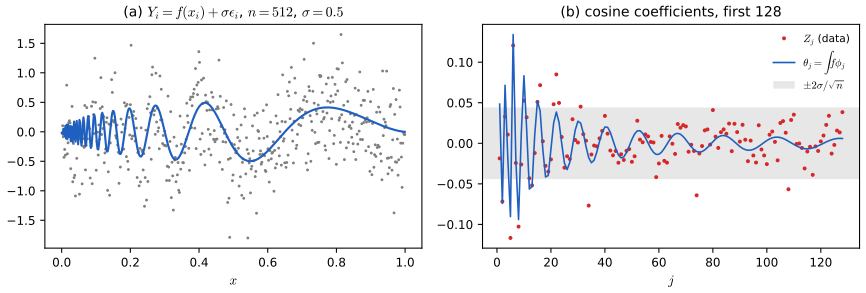
fig_7_S1, regression_coefficients. Supplementary figure (the book has no figure here). Download: PDF · SVGDensity estimation also reduces to the Normal means model, but for the square root of the density (Nussbaum 1996a); the white noise model of the appendix is the cleanest continuous version. In the precise sense of Le Cam's deficiency distance these experiments are asymptotically equivalent (Brown and Low 1996; Nussbaum 1996a), so minimax results proved for the sequence model transfer to them.
See also (companion course): orthogonal series regression in Probability and Statistical Inference.
7.4 Stein's Unbiased Risk Estimator (SURE)
pp. 150–153 Cross-validation estimates risk by refitting; in the Normal means model there is an exact, refit-free alternative.
Theorem 7.17 (Stein 1981) p. 151, (7.18)–(7.19)
Let \(Z\sim N_n(\theta,V)\), let \(\hth=\hth(Z)\) and \(g(z)=\hth(z)-z\), a map \(\R^n\to\R^n\). Let \(D\) be the matrix \(D_{ij}=\partial g_i/\partial z_j\) and
\[ \sure(z)=\Tr(V)+2\Tr(VD)+\sum_ig_i^2(z). \tag{7.18} \]If \(g\) is weakly differentiable (and \(\E_\theta|\partial_jg_i(Z)|\lt \infty\)), then \(\E_\theta\sure(Z)=R(\hth,\theta)\). In the model (7.1), \(V=\sn^2I\) and
\[ \sure(z)=n\sn^2+2\sn^2\sum_{i=1}^nD_{ii}+\sum_{i=1}^ng_i^2. \tag{7.19} \]Filling the gap 7.3: Stein's lemma (Exercise 4) and the proof of Theorem 7.17 for general \(V\) pp. 151–152
The whole theorem rests on one integration by parts: \(\E[g(X)(X-\mu)]=\sigma^2\E g'(X)\) for \(X\sim N(\mu,\sigma^2)\). The book proves the case \(V=\sigma^2I\); here is the general case.
Proof
Stein's lemma. Let \(X\sim N(\mu,\sigma^2)\) with density \(\varphi\), and let \(g\) be weakly differentiable (absolutely continuous on bounded intervals, with derivative \(g'\)) with \(\E|g'(X)|\lt \infty\). Since \(\varphi'(x)=-\frac{x-\mu}{\sigma^2}\varphi(x)\),
\[ \E[g(X)(X-\mu)]=-\sigma^2\int g(x)\varphi'(x)\,\d x. \]Write \(g(x)=g(\mu)+\int_\mu^xg'(t)\d t\). The constant contributes \(-\sigma^2g(\mu)\int\varphi'=0\). For the rest, by Fubini (justified by \(\E|g'(X)|\lt \infty\), see below),
\[ -\int_\mu^\infty\!\!\int_\mu^xg'(t)\,\d t\,\varphi'(x)\,\d x=\int_\mu^\infty g'(t)\Big(-\int_t^\infty\varphi'(x)\d x\Big)\d t=\int_\mu^\infty g'(t)\varphi(t)\,\d t, \]and the same on \((-\infty,\mu)\). Together, \(\E[g(X)(X-\mu)]=\sigma^2\int g'\varphi=\sigma^2\E g'(X)\). Fubini applies because \(\int_\mu^\infty\int_\mu^x|g'(t)||\varphi'(x)|\d t\,\d x=\int_\mu^\infty|g'(t)|\varphi(t)\d t\lt \infty\) (on \(x>\mu\), \(\varphi'\lt 0\) and \(\int_t^\infty|\varphi'|=\varphi(t)\)). This is Exercise 4; the companion course proves it the same way (Lemma 12.C).
Multivariate version. If \(Z\sim N_n(\theta,\sigma^2I)\), apply the lemma to coordinate \(i\) conditionally on the others: \(\E[g_i(Z)(Z_i-\theta_i)]=\sigma^2\E[\partial g_i/\partial z_i]\). For general \(V\) (positive definite), write \(Z=\theta+V^{1/2}W\), \(W\sim N(0,I)\). For a scalar weakly differentiable \(h\), \(\E[h(Z)W]=\E[\nabla_w h(\theta+V^{1/2}W)]=V^{1/2}\E\nabla h(Z)\) by the identity-covariance case, hence \(\E[h(Z)(Z-\theta)]=V^{1/2}\E[h(Z)W]=V\E\nabla h(Z)\). Applying this to \(h=g_i\) and summing the \(i\)th components gives
\[ \E[g(Z)^\T(Z-\theta)]=\sum_{i,j}V_{ij}\E\,\partial_jg_i(Z)=\E\Tr(VD). \]Unbiasedness. Expand \(\|\hth-\theta\|^2=\|g(Z)+(Z-\theta)\|^2=\|g\|^2+2g^\T(Z-\theta)+\|Z-\theta\|^2\). Taking expectations, \(\E\|Z-\theta\|^2=\Tr V\) and \(\E[2g^\T(Z-\theta)]=2\E\Tr(VD)\), so \(R(\hth,\theta)=\E[\Tr V+2\Tr(VD)+\|g\|^2]=\E\sure(Z)\). (The book's display writes \(\Tr(V)\) where it means the constant \(\Tr V\), and its proof uses \(n\sigma^2\) for \(n\sn^2\); the argument is the one above.)
Example 7.20: SURE for three estimators
p. 152 With \(V=\sn^2I\) (write \(\sigma=\sn\)):
- \(\hth=Z\): \(g=0\), \(\sure=n\sigma^2\), the true risk.
- \(\hth=bZ\): \(g=(b-1)Z\), \(D_{ii}=b-1\), so \(\sure=(2b-1)n\sigma^2+(1-b)^2\sum_iZ_i^2\).
- Soft thresholding,
has SURE (Exercise 5)
\[ \sure(Z)=\sum_{i=1}^n\big[\sigma^2-2\sigma^2\I(|Z_i|\le\lambda)+\min(Z_i^2,\lambda^2)\big]. \tag{7.22} \]Hard thresholding,
\[ \hth_i=\begin{cases}Z_i,&|Z_i|>\lambda\\0,&|Z_i|\le\lambda,\end{cases} \tag{7.23} \]jumps at \(\pm\lambda\), so it is not weakly differentiable (Exercise 6) and (7.19) does not apply: the "derivative" contains point masses at \(\pm\lambda\) that the formula would miss.
Why (7.22) holds Exercise 5
For soft thresholding \(g_i=-\lambda\sign(Z_i)\) when \(|Z_i|>\lambda\) and \(g_i=-Z_i\) when \(|Z_i|\le\lambda\), so \(g_i^2=\min(Z_i^2,\lambda^2)\). The function \(z\mapsto\sign(z)(|z|-\lambda)_+-z\) is continuous and piecewise linear, hence weakly differentiable, with derivative \(D_{ii}=-\I(|Z_i|\le\lambda)\) (the value at the two kinks is irrelevant). Substituting in (7.19) gives (7.22). Figure 7.S2(b) shows that SURE tracks the exact risk of Exercise 7 as a function of \(\lambda\), and that its minimiser is close to the best threshold.
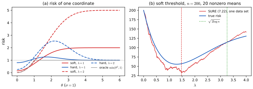
fig_7_S2, sure_soft, risk_soft, risk_hard. Supplementary figure. Download: PDF · SVGExample 7.24: model selection
pp. 152–153 For \(S\subset\{1,\dots,n\}\) let
\[ \hth_S=(Z_i\I(i\in S))_{i=1}^n, \tag{7.25} \]the estimator under the submodel "\(\theta_i=0\) for \(i\notin S\)". Its risk is \(R(\hth_S,\theta)=\sn^2|S|+\sum_{i\notin S}\theta_i^2\) (variance of the kept coordinates plus squared bias of the killed ones). Replacing \(\theta_i^2\) by its unbiased estimate \(Z_i^2-\sn^2\) gives
\[ \sure_S=\sn^2|S|+\sum_{i\in S^c}(Z_i^2-\sn^2), \tag{7.26} \]which is (7.19) for this estimator (\(g_i=-Z_i\I(i\notin S)\), \(D_{ii}=-\I(i\notin S)\)) and is Mallows' \(C_p\) up to a constant. Minimising \(\sure_S\) over a class \(\mathcal S\) of subsets is model selection: over the nested class \(\{\emptyset,\{1\},\{1,2\},\dots\}\) it chooses a cut-off; over all subsets it keeps exactly the coordinates with \(Z_i^2>2\sn^2\), a hard threshold at \(\sqrt2\sn\). Unbiasedness for each fixed \(S\) does not make the minimum over many \(S\) reliable; Exercise 10 quantifies the uniform error.
See also (companion course): \(C_p\) and AIC and the effective number of parameters, \(\sum_i\partial\hth_i/\partial Z_i\), in Statistical Learning: Theory and Methods.
7.5 Minimax Risk and Pinsker's Theorem
pp. 153–155 For \(\Theta_n\subset\R^n\) the minimax risk is
\[ R_n\equiv R(\Theta_n)\equiv\inf_{\hth}\sup_{\theta\in\Theta_n}R(\hth,\theta), \tag{7.27} \]the infimum running over all estimators. The first case is the \(L_2\) ball \(\Theta_n(c)=\{\theta\in\R^n:\sum_i\theta_i^2\le c^2\}\).
Theorem 7.28 (Pinsker's theorem for the ball) p. 153, (7.29)
In model (7.1) with \(\sn^2=\sigma^2/n\), for every \(c>0\),
\[ \liminf_{n\to\infty}\ \inf_{\hth}\sup_{\theta\in\Theta_n(c)}R(\hth,\theta)=\frac{\sigma^2c^2}{\sigma^2+c^2}. \tag{7.29} \]In fact \(R_n\le\sigma^2c^2/(\sigma^2+c^2)\) for every \(n\), so the limit exists and equals the right side. The MLE has risk \(\sigma^2\), strictly larger.
The idea: the linear estimator \(\hth_j=c^2Z_j/(\sigma^2+c^2)\) has worst-case risk
\[ R_n\le\frac{\sigma^2c^2}{\sigma^2+c^2}, \tag{7.30} \]and if a prior \(\pi\) on \(\Theta_n(c)\) had Bayes risk equal to this value, then for every estimator
\[ \frac{\sigma^2c^2}{\sigma^2+c^2}=\int R(\hth_\pi,\theta)\,\d\pi(\theta)\le\int R(\hth,\theta)\,\d\pi(\theta)\le\sup_{\theta\in\Theta_n}R(\hth,\theta), \tag{7.31} \]and taking the infimum over \(\hth\) would give \(R_n\) exactly. No prior on the ball does this for finite \(n\), but the Gaussian prior \(\theta_i\sim N(0,c^2\delta^2/n)\) nearly lives on the ball for large \(n\), because \(\|\theta\|^2\) concentrates at \(c^2\delta^2\lt c^2\).
Filling the gap 7.4: a complete proof of Theorem 7.28 pp. 153–154 and 174–176
The book's appendix proof follows Nussbaum (1996b). Three steps need justification: why one may restrict to estimators with values in the ball, the chi-square deviation inequality, and the bookkeeping of the error terms.
Proof
Upper bound, for every \(n\). Let \(w=c^2/(\sigma^2+c^2)\) and \(\hth=wZ\). Each coordinate has bias \(-(1-w)\theta_j\) and variance \(w^2\sigma^2/n\), so
\[ R(\hth,\theta)=(1-w)^2\|\theta\|^2+w^2\sigma^2=\frac{\sigma^4\|\theta\|^2+\sigma^2c^4}{(\sigma^2+c^2)^2}\le\frac{\sigma^4c^2+\sigma^2c^4}{(\sigma^2+c^2)^2}=\frac{\sigma^2c^2}{\sigma^2+c^2} \]on \(\|\theta\|\le c\). Hence \(R_n\le\sigma^2c^2/(\sigma^2+c^2)\).
Step 1: estimators with values in the ball suffice. Let \(P\) be the Euclidean projection onto the closed convex set \(\Theta_n(c)\), \(P(v)=v\min(1,c/\|v\|)\). Projection onto a closed convex set is 1-Lipschitz and fixes its points, so for \(\theta\in\Theta_n(c)\), \(\|P(\hth)-\theta\|=\|P(\hth)-P(\theta)\|\le\|\hth-\theta\|\). Hence \(\sup_{\Theta_n}R(P\hth,\theta)\le\sup_{\Theta_n}R(\hth,\theta)\), and \(R_n\) is also the infimum over estimators with values in \(\Theta_n(c)\).
Step 2: a Bayes lower bound. Fix \(\delta\in(1/\sqrt2,1)\) and let \(\pi_n\) make \(\theta_1,\dots,\theta_n\) iid \(N(0,\tau^2)\), \(\tau^2=c^2\delta^2/n\). The posterior of \(\theta_j\) given \(Z\) is Normal with mean \(\tau^2Z_j/(\tau^2+\sn^2)=c^2\delta^2Z_j/(c^2\delta^2+\sigma^2)\) and variance \(\tau^2\sn^2/(\tau^2+\sn^2)\), so the Bayes risk is
\[ B(\pi_n)=n\cdot\frac{\tau^2\sn^2}{\tau^2+\sn^2}=\frac{\sigma^2c^2\delta^2}{\sigma^2+c^2\delta^2}. \]For any estimator \(\tilde\theta\) with values in \(\Theta_n(c)\), splitting the integral over \(\Theta_n\) and its complement,
\[ B(\pi_n)\le\int R(\tilde\theta,\theta)\,\d\pi_n\le\sup_{\theta\in\Theta_n}R(\tilde\theta,\theta)+\int_{\Theta_n^c}\E_\theta\|\tilde\theta-\theta\|^2\,\d\pi_n(\theta). \]Since \(\|\tilde\theta\|\le c\), \(\|\tilde\theta-\theta\|^2\le2c^2+2\|\theta\|^2\), and by Cauchy–Schwarz
\[ \int_{\Theta_n^c}\E_\theta\|\tilde\theta-\theta\|^2\d\pi_n\le2c^2\pi_n(\Theta_n^c)+2\sqrt{\pi_n(\Theta_n^c)}\,\sqrt{\E_{\pi_n}\|\theta\|^4}=:\Delta_n, \]which does not depend on \(\tilde\theta\). Taking the infimum over \(\tilde\theta\) and using Step 1, \(R_n\ge B(\pi_n)-\Delta_n\). (The book takes a supremum over all estimators of the second term, which is infinite unless the estimators are restricted as in Step 1.)
Step 3: \(\Delta_n\to0\). Under \(\pi_n\), \(\|\theta\|^2=\tau^2W\) with \(W\sim\chi^2_n\), so \(\E\|\theta\|^4=\tau^4(n^2+2n)=c^4\delta^4(1+2/n)\), bounded. And \(\pi_n(\Theta_n^c)=\P(W>n/\delta^2)=\P(W/n-1>t)\) with \(t=1/\delta^2-1\in(0,1)\). The deviation inequality used in the book,
\[ \P\Big(\Big|\frac1n\sum_{j=1}^n(\xi_j^2-1)\Big|>t\Big)\le2e^{-nt^2/8},\qquad 0\lt t\lt 1,\ \xi_j\ \text{iid}\ N(0,1), \]follows from Chernoff's bound. For \(0\lt \lambda\lt 1/2\), \(\log\E e^{\lambda(\xi^2-1)}=-\lambda-\tfrac12\log(1-2\lambda)=\sum_{k\ge2}(2\lambda)^k/(2k)\le\sum_{k\ge2}(2\lambda)^k/4=\lambda^2/(1-2\lambda)\). Markov's inequality then gives \(\P(\frac1n\sum(\xi_j^2-1)>t)\le\exp(-n[\lambda t-\lambda^2/(1-2\lambda)])\); with \(\lambda=t/4\le1/4\), \(\lambda^2/(1-2\lambda)\le2\lambda^2=t^2/8\) and the exponent is at least \(n(t^2/4-t^2/8)=nt^2/8\). For the lower tail, \(\log\E e^{-\lambda(\xi^2-1)}=\lambda-\tfrac12\log(1+2\lambda)=\sum_{k\ge2}(-1)^k(2\lambda)^k/(2k)\le\lambda^2\) (alternating series with decreasing terms), and \(\lambda=t/2\) gives \(e^{-nt^2/4}\le e^{-nt^2/8}\). So \(\pi_n(\Theta_n^c)\le e^{-nt^2/8}\to0\) exponentially fast, and \(\Delta_n\to0\).
Conclusion. \(\liminf_nR_n\ge\sigma^2c^2\delta^2/(\sigma^2+c^2\delta^2)\) for every \(\delta\lt 1\); let \(\delta\uparrow1\) and combine with the upper bound. The same Bayes-plus-concentration argument, with a fixed number of means and no concentration step, is the companion course's Filling the gap 12.13.
Now the smooth-function version: by Theorem 7.11, a class of periodic functions with \(\|D^mf\|\le c\) is a Sobolev ellipsoid of coefficients.
Theorem 7.32 (Pinsker's theorem for Sobolev ellipsoids) p. 154, (7.33)–(7.35)
Let
\[ Z_j=\theta_j+\frac{\sigma}{\sqrt n}\epsilon_j,\qquad j=1,2,\dots, \tag{7.33} \]with \(\theta\in\Theta(m,c)\). The minimax risk \(R_n\) over \(\Theta(m,c)\) satisfies
\[ \lim_{n\to\infty}n^{2m/(2m+1)}R_n=\Big(\frac{\sigma^2}{\pi}\Big)^{2m/(2m+1)}c^{2/(2m+1)}P_m, \tag{7.34} \] \[ P_m=\Big(\frac{m}{m+1}\Big)^{2m/(2m+1)}(2m+1)^{1/(2m+1)}, \tag{7.35} \]the Pinsker constant. (The book prints \((\sigma/\pi)^{2m/(2m+1)}\); the correct power of \(\sigma\) is 2, see Filling the gap 7.6 and the note.) Hence the minimax rate is \(n^{-2m/(2m+1)}\): \(0\lt \lim n^{2m/(2m+1)}R_n\lt \infty\).
Theorem 7.36 (Pinsker's theorem for ellipsoids) pp. 154–155
Let \(\Theta=\{\theta:\sum_ja_j^2\theta_j^2\le c^2\}\) with \(a_j\ge0\), \(a_j\to\infty\) (the book writes \(\sum_ja_j\theta_j^2\); the formulas below hold with \(a_j^2\), as in (7.9)), and observations \(Z_j=\theta_j+\sn\epsilon_j\). Let \(R_n^L=\inf_{\hth\in\mathcal L}\sup_\Theta R(\hth,\theta)\) be the minimax risk over linear estimators \(\hth=(w_1Z_1,w_2Z_2,\dots)\). Then
- linear estimators are asymptotically minimax: \(R_n\sim R_n^L\) as \(\sn\to0\);
- \(\displaystyle R_n^L=\sn^2\sum_i\Big(1-\frac{a_i}{\mu}\Big)_+\), where \(\mu\) solves \(\displaystyle\sn^2\sum_ia_i(\mu-a_i)_+=c^2\);
- the linear minimax estimator is \(\hth_i=w_iZ_i\), \(w_i=(1-a_i/\mu)_+\);
- it is the Bayes estimator for independent \(\theta_i\sim N(0,\tau_i^2)\), \(\tau_i^2=\sn^2(\mu/a_i-1)_+\).
Filling the gap 7.5: proof of Theorem 7.36 pp. 154–155
Parts (2)–(4) are an exact finite computation: the worst case of a linear estimator over an ellipsoid puts all the energy on one coordinate, and minimising the resulting max-plus-sum gives the "water-filling" weights. Part (1) repeats the Bayes-plus-concentration argument of Filling the gap 7.4 with the prior of part (4).
Proof
Worst case of a linear estimator. For \(\hth_i=w_iZ_i\), \(R(\hth,\theta)=\sum_i(1-w_i)^2\theta_i^2+\sn^2\sum_iw_i^2\). Put \(u_i=a_i^2\theta_i^2\ge0\) with \(\sum u_i\le c^2\); the first sum is \(\sum_iu_i(1-w_i)^2/a_i^2\), a linear function of \(u\) on a simplex, maximised by putting all of \(c^2\) on the largest coefficient. So
\[ \sup_{\theta\in\Theta}R(\hth,\theta)=\sn^2\sum_iw_i^2+c^2\sup_i\frac{(1-w_i)^2}{a_i^2} \](with the convention that a coordinate with \(a_i=0\) forces \(w_i=1\), otherwise the supremum is infinite).
Minimising. Fix the value \(M=\sup_i(1-w_i)^2/a_i^2=1/\mu^2\). The constraint is \(|1-w_i|\le a_i/\mu\) for every \(i\), and \(\sum w_i^2\) is smallest when each \(w_i\) is as close to 0 as allowed: \(w_i=(1-a_i/\mu)_+\). The risk becomes
\[ F(\mu)=\sn^2\sum_i\Big(1-\frac{a_i}{\mu}\Big)_+^2+\frac{c^2}{\mu^2}, \]a finite sum for each \(\mu\) because \(a_i\to\infty\). Differentiating (each term is \(C^1\) in \(\mu\)), \(F'(\mu)=\frac{2}{\mu^3}\big[\sn^2\sum_ia_i(\mu-a_i)_+-c^2\big]\). The bracket is continuous, strictly increasing once \(\mu\) exceeds the smallest \(a_i\), zero for small \(\mu\) and unbounded, so \(F\) decreases then increases and its minimiser is the unique root of \(\sn^2\sum a_i(\mu-a_i)_+=c^2\): this is (2)–(3). At the root, \(c^2/\mu^2=\sn^2\sum_i(a_i/\mu)(1-a_i/\mu)_+\), and adding,
\[ R_n^L=F(\mu)=\sn^2\sum_i\Big(1-\frac{a_i}{\mu}\Big)_+\Big[\Big(1-\frac{a_i}{\mu}\Big)+\frac{a_i}{\mu}\Big]=\sn^2\sum_i\Big(1-\frac{a_i}{\mu}\Big)_+. \](4) Bayes. Under \(\theta_i\sim N(0,\tau_i^2)\) independently, the posterior mean is \(\frac{\tau_i^2}{\tau_i^2+\sn^2}Z_i\), and with \(\tau_i^2=\sn^2(\mu/a_i-1)_+\) the weight is \(\frac{\mu/a_i-1}{\mu/a_i}=1-a_i/\mu\) when positive, and 0 otherwise. The Bayes risk is \(\sum_i\tau_i^2\sn^2/(\tau_i^2+\sn^2)=\sn^2\sum_i(1-a_i/\mu)_+=R_n^L\), and the prior satisfies \(\E\sum a_i^2\theta_i^2=\sn^2\sum_ia_i(\mu-a_i)_+=c^2\): it sits on the boundary of the ellipsoid on average. It is the least favourable Gaussian prior.
(1) Asymptotic minimaxity. Clearly \(R_n\le R_n^L\). For the lower bound fix \(\delta\lt 1\) and use the prior \(\theta_i\sim N(0,\delta^2\tau_i^2)\). Its Bayes risk is \(\sum_i\delta^2\tau_i^2\sn^2/(\delta^2\tau_i^2+\sn^2)\ge\delta^2R_n^L\). As in Filling the gap 7.4 (project estimators onto the convex set \(\Theta\); bound the risk off \(\Theta\) with Cauchy–Schwarz), \(R_n\ge\delta^2R_n^L-\Delta_n\) with \(\Delta_n\) controlled by \(\pi(\Theta^c)\) and \(\E\|\theta\|^4\). Now \(\sum a_i^2\theta_i^2\) has mean \(\delta^2c^2\) and variance \(2\delta^4\sum_ia_i^4\tau_i^4\le2\delta^4c^2\max_ia_i^2\tau_i^2\). For Sobolev ellipsoids the number of nonzero \(\tau_i\) grows like \(n^{1/(2m+1)}\) and \(\max_ia_i^2\tau_i^2/c^2\to0\), so by Chebyshev \(\pi(\Theta^c)=\P(\sum a_i^2\theta_i^2>c^2)\to0\); the same weighted-chi-square Chernoff bound as before makes it small compared with \(R_n^L\). Hence \(\liminf R_n/R_n^L\ge\delta^2\) for every \(\delta\lt 1\). The argument is Pinsker's (1980); Johnstone's monograph gives it in this form.
A remark on the book's display. If the ellipsoid is written \(\sum a_j\theta_j^2\le c^2\), as in the book's statement, the formulas hold with \(\sqrt{a_j}\) in place of \(a_j\); taken literally with \(a_j\) they give a different (wrong) answer. This was confirmed numerically: on a test ellipsoid, the worst-case risk of the weights \((1-a_j/\mu)_+\) equals \(\sn^2\sum(1-a_j/\mu)_+\) exactly for the constraint \(\sum a_j^2\theta_j^2\le c^2\), and no random perturbation of the weights does better.
Filling the gap 7.6: Theorem 7.32 from Theorem 7.36, and where the Pinsker constant comes from p. 154
Replace the sums in Theorem 7.36 by integrals: the active coefficients are those with \(a_j\lt \mu\), about \(\mu^{1/m}/\pi\) of them.
Derivation
Take \(a_j\approx(\pi j)^m\) (the pairing \(a_{2j}=a_{2j+1}\) of Theorem 7.11 changes nothing to first order, since the number of indices with \(a_j\lt \mu\) is still \(\mu^{1/m}/\pi+O(1)\)). Let \(J=\mu^{1/m}/\pi\), \(\varepsilon^2=\sigma^2/n\). Comparing sums with integrals of monotone functions, with relative error \(O(1/J)\),
\[ \sum_ja_j(\mu-a_j)_+\approx\int_0^J(\pi x)^m\big(\mu-(\pi x)^m\big)\d x=\frac{\mu^{(2m+1)/m}}{\pi}\Big(\frac1{m+1}-\frac1{2m+1}\Big)=\frac{m\,\mu^{(2m+1)/m}}{\pi(m+1)(2m+1)}. \]Setting \(\varepsilon^2\) times this equal to \(c^2\) gives \(\mu^{1/m}=\big[\pi c^2(m+1)(2m+1)/(m\varepsilon^2)\big]^{1/(2m+1)}\to\infty\), so \(J\to\infty\) and the approximation becomes exact in the limit. Similarly
\[ R_n^L=\varepsilon^2\sum_j\Big(1-\frac{a_j}{\mu}\Big)_+\approx\varepsilon^2\int_0^J\Big(1-\frac{(\pi x)^m}{\mu}\Big)\d x=\varepsilon^2J\frac{m}{m+1}. \]Substituting \(J\):
\[ R_n^L\approx\frac{\varepsilon^2}{\pi}\frac{m}{m+1}\Big[\frac{\pi c^2(m+1)(2m+1)}{m\varepsilon^2}\Big]^{\frac1{2m+1}}=\Big(\frac{\varepsilon^2}{\pi}\Big)^{\frac{2m}{2m+1}}c^{\frac2{2m+1}}\Big(\frac m{m+1}\Big)^{\frac{2m}{2m+1}}(2m+1)^{\frac1{2m+1}}. \]With \(\varepsilon^2=\sigma^2/n\) this is \(n^{-2m/(2m+1)}(\sigma^2/\pi)^{2m/(2m+1)}c^{2/(2m+1)}P_m\), and by Theorem 7.36(1) \(R_n\sim R_n^L\). The power of \(\sigma\) is \(2\cdot\frac{2m}{2m+1}\): the book's \((\sigma/\pi)^{2m/(2m+1)}\) is right only when \(\sigma=1\). Figure 7.S4(b) computes \(n^{2m/(2m+1)}R_n^L\) exactly for \(\sigma=2\) and shows it converging to the \(\sigma^2/\pi\) limit (1.067 for \(m=1\), 1.210 for \(m=2\)), not to the book's (0.672 and 0.695).
Reading the rate. The estimator keeps about \(J\asymp(nc^2/\sigma^2)^{1/(2m+1)}\) coefficients, each with variance \(\sigma^2/n\), and the bias from the rest is of the same order: \(J\sigma^2/n\asymp n^{-2m/(2m+1)}\). For \(m=2\) this is the familiar \(n^{-4/5}\) of kernel smoothing (Chapters 5 and 6).
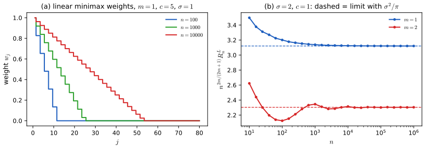
fig_7_S4, pinsker_linear, pinsker_limit. Supplementary figure. Download: PDF · SVGSee also (companion course): a Bayes rule with constant risk is minimax and the ball version of this argument in Probability and Statistical Inference.
7.6 Linear Shrinkage and the James–Stein Estimator
pp. 155–158 Back to model (7.1). A linear shrinkage estimator is \(\hth=bZ\), \(b\in[0,1]\); the class is \(\mathcal L=\{bZ:b\in[0,1]\}\). By the bias–variance decomposition,
\[ R(bZ,\theta)=(1-b)^2\|\theta\|_n^2+nb^2\sn^2, \tag{7.37} \]with \(\|\theta\|_n^2=\sum_{i=1}^n\theta_i^2\). This quadratic in \(b\) is minimised at \(b_*=\|\theta\|_n^2/(n\sn^2+\|\theta\|_n^2)\), the ideal linear estimator, with risk
\[ R(b_*Z,\theta)=\frac{n\sn^2\|\theta\|_n^2}{n\sn^2+\|\theta\|_n^2}. \tag{7.38} \]Theorem 7.39 (the linear oracle risk) p. 155, (7.40)
\[ \inf_{\hth\in\mathcal L}R(\hth,\theta)=\frac{n\sn^2\|\theta\|_n^2}{n\sn^2+\|\theta\|_n^2}. \tag{7.40} \](Setting the derivative \(-2(1-b)\|\theta\|^2+2nb\sn^2\) to zero gives \(b_*\in[0,1)\); substituting gives (7.38).) Only an oracle that knows \(\|\theta\|\) can use \(b_*\).
The James–Stein estimator estimates \(b_*\) from the data:
\[ \hth^{\JS}=\Big(1-\frac{(n-2)\sn^2}{\sum_{i=1}^nZ_i^2}\Big)Z. \tag{7.41} \]Theorem 7.42 (risk bound for James–Stein) p. 156, (7.43)–(7.44)
For \(n\ge3\) and every \(\theta\in\R^n\), the exact risk is
\[ R(\hth^{\JS},\theta)=n\sn^2-(n-2)^2\sn^4\,\E_\theta\Big(\frac1{\sum_iZ_i^2}\Big), \tag{7.44} \]and it satisfies
\[ R(\hth^{\JS},\theta)\le2\sn^2+\frac{(n-2)\sn^2\|\theta\|_n^2}{(n-2)\sn^2+\|\theta\|_n^2}\le2\sn^2+\frac{n\sn^2\|\theta\|_n^2}{n\sn^2+\|\theta\|_n^2}. \tag{7.43} \]Filling the gap 7.7: the exact risk of James–Stein, the Poisson mixture, and the positive part pp. 156–157
Three facts the proof quotes: SURE for (7.41), the representation of a noncentral chi-square as a Poisson mixture of central ones, and \(\E(1/\chi^2_k)=1/(k-2)\). With them, the risk (7.44) can be computed exactly; Figure 7.S3 plots it.
Proof
SURE. Write \(\hth^{\JS}=Z+g(Z)\), \(g(z)=-(n-2)\sn^2z/S\), \(S=\sum_kz_k^2\). Then \(\partial g_i/\partial z_i=-(n-2)\sn^2\big(1/S-2z_i^2/S^2\big)\), and summing over \(i\), \(\sum_iD_{ii}=-(n-2)\sn^2(n-2)/S\). With \(\sum g_i^2=(n-2)^2\sn^4/S\), (7.19) gives
\[ \sure(Z)=n\sn^2-\frac{2(n-2)^2\sn^4}{S}+\frac{(n-2)^2\sn^4}{S}=n\sn^2-\frac{(n-2)^2\sn^4}{S}. \]The function \(g\) is smooth away from 0 and \(\E|D_{ii}|\le C\E(1/S)\lt \infty\) for \(n\ge3\), so Theorem 7.17 applies and (7.44) follows. In particular \(R(\hth^{\JS},\theta)\lt n\sn^2\) for every \(\theta\): James–Stein dominates the MLE for \(n\ge3\) (Stein's paradox; the companion course proves this in Theorem 12.D).
The Poisson mixture. \(S/\sn^2=\sum_i(\theta_i/\sn+\epsilon_i)^2\) is noncentral \(\chi^2_{\delta,n}\) with \(\delta=\|\theta\|^2/\sn^2\). Rotate so that the mean vector points along the first axis (the distribution of \(\epsilon\) is rotation invariant): \(S/\sn^2\overset d=(\sqrt\delta+\epsilon_1)^2+\chi^2_{n-1}\). For \(s\lt 1/2\), completing the square,
\[ \E e^{s(\sqrt\delta+\epsilon_1)^2}=\frac{1}{\sqrt{1-2s}}\exp\Big(\frac{\delta s}{1-2s}\Big)=\frac{e^{-\delta/2}}{\sqrt{1-2s}}\exp\Big(\frac{\delta/2}{1-2s}\Big)=\sum_{k\ge0}e^{-\delta/2}\frac{(\delta/2)^k}{k!}(1-2s)^{-(2k+1)/2}. \]Multiplying by the moment generating function \((1-2s)^{-(n-1)/2}\) of \(\chi^2_{n-1}\), the mgf of \(S/\sn^2\) is \(\sum_k\P(K=k)(1-2s)^{-(n+2k)/2}\), \(K\sim\mathrm{Poisson}(\delta/2)\): the mgf of \(\chi^2_{n+2K}\). Moment generating functions finite on an interval determine the distribution, so \(S/\sn^2\overset d=\chi^2_{n+2K}\).
The inverse moment. For \(k>2\), \(\E(1/\chi^2_k)=\int_0^\infty x^{k/2-2}e^{-x/2}\d x\big/\big(2^{k/2}\Gamma(k/2)\big)=2^{k/2-1}\Gamma(k/2-1)/(2^{k/2}\Gamma(k/2))=1/(k-2)\). Hence, conditioning on \(K\),
\[ \E_\theta\frac1S=\frac1{\sn^2}\E\Big[\frac1{n-2+2K}\Big]\ge\frac1{\sn^2}\cdot\frac1{n-2+\delta}=\frac1{(n-2)\sn^2+\|\theta\|^2}, \]by Jensen's inequality (\(x\mapsto1/(n-2+2x)\) is convex and \(\E K=\delta/2\)). Substituting in (7.44) gives \(R\le n\sn^2-(n-2)^2\sn^4/((n-2)\sn^2+\|\theta\|^2)\), and writing \(n\sn^2=2\sn^2+(n-2)\sn^2\) and combining the last two terms gives the first inequality of (7.43). The second holds because \(x\mapsto x\|\theta\|^2/(x+\|\theta\|^2)\) is increasing in \(x\). The exact series \(\sum_kP(K=k)/(n-2+2k)\) is what the code and the demonstration evaluate; it agrees with simulation to Monte Carlo accuracy. At \(\theta=0\) it gives \(R=n\sn^2-(n-2)\sn^2=2\sn^2\) exactly.
Remark 7.45: the positive part cannot hurt. Let \(b(Z)=1-c/\|Z\|^2\) and \(b_+=\max(b,0)\). Then
\[ \|bZ-\theta\|^2-\|b_+Z-\theta\|^2=(b^2-b_+^2)\|Z\|^2-2(b-b_+)\theta^\T Z, \]which is zero when \(b\ge0\) and equals \(b^2\|Z\|^2-2b\,\theta^\T Z\) when \(b\lt 0\). The event \(\{b\lt 0\}\) depends on \(Z\) only through \(\|Z\|\), and given \(\|Z\|=r\) the conditional law of \(Z\) on the sphere has density proportional to \(\exp(\theta^\T z/\sn^2)\), a tilt towards \(\theta\), so \(\E[\theta^\T Z\given\|Z\|=r]\ge0\) (the tilted mean of \(\theta^\T z\) under a symmetric base law is nonnegative, by the covariance inequality for the increasing functions \(u\mapsto u\) and \(u\mapsto e^{u/\sn^2}\) of \(u=\theta^\T z\)). Since \(-2b>0\) on \(\{b\lt 0\}\), the expected difference is nonnegative: the positive-part estimator (7.46) has risk no larger than the plain one, for any \(c\). The simulated positive-part risk in Figure 7.S3's demonstration lies below the exact James–Stein curve, most visibly near \(\theta=0\).
Remark 7.45 (modified James–Stein) p. 157, (7.46)
\[ \hth=\Big(1-\frac{n\sn^2}{\sum_iZ_i^2}\Big)_+Z. \tag{7.46} \]Replacing \(n-2\) by \(n\) changes little for large \(n\), and the positive part never increases the risk (proof in Filling the gap 7.7). This is the version used in practice and in Exercise 1.
Theorem 7.47 (James–Stein oracle inequality) p. 157
With \(\mathcal L=\{bZ:b\in\R\}\), for every \(\theta\in\R^n\), \(n\ge3\),
\[ \inf_{\hth\in\mathcal L}R(\hth,\theta)\le R(\hth^{\JS},\theta)\le2\sn^2+\inf_{\hth\in\mathcal L}R(\hth,\theta). \]The right inequality is (7.43) combined with (7.40). The left one is not automatic, because \(\hth^{\JS}=\hat bZ\) uses a data-dependent \(\hat b\), and a data-dependent factor could in principle beat the best fixed one; the book says it "follows from (7.38) and Theorem 7.42", but neither gives a lower bound. Filling the gap 7.8 proves it.
Another view of James–Stein: SURE for \(bZ\) is \(n\sn^2+2n\sn^2(b-1)+(b-1)^2\sum_iZ_i^2\), minimised at \(\hat b=1-n\sn^2/\sum_iZ_i^2\). Plugging in gives \((1-n\sn^2/\sum Z_i^2)Z\): James–Stein with \(n\) in place of \(n-2\), i.e. the estimator (7.46) without the positive part. So James–Stein is the SURE-optimal linear shrinkage.
Theorem 7.48 (James–Stein is asymptotically minimax) p. 157
With \(\sn^2=\sigma^2/n\),
\[ \lim_{n\to\infty}\sup_{\theta\in\Theta_n(c)}R(\hth^{\JS},\theta)=\frac{\sigma^2c^2}{\sigma^2+c^2}. \]Remark 7.49 (adaptivity) p. 158
James–Stein achieves the minimax risk over every ball \(\Theta_n(c)\) without knowing \(c\). It is essentially the best linear shrinkage for every \(\theta\), and asymptotically the best of all estimators over balls; in particular the minimax and the linear minimax risks over balls coincide asymptotically.
Filling the gap 7.8: the left inequality of Theorem 7.47, and the proof of Theorem 7.48 pp. 157–158
The left inequality reduces to an inequality for a Poisson expectation, proved with the Poisson identity \(\lambda\E h(K+1)=\E[Kh(K)]\).
Proof
Left inequality of Theorem 7.47. Write \(\sigma=\sn\), \(t^2=\|\theta\|^2\), \(\delta=t^2/\sigma^2\), \(m=n-2\ge1\), \(K\sim\mathrm{Poisson}(\lambda)\), \(\lambda=\delta/2\). By (7.44) and Filling the gap 7.7, \(R(\hth^{\JS},\theta)=n\sigma^2-m^2\sigma^2\E[1/(m+2K)]\), and by (7.38) \(\inf_{\mathcal L}R=n\sigma^2-n^2\sigma^2/(n+\delta)\). So the claim is
\[ (n+\delta)\,\E\Big[\frac1{m+2K}\Big]\le\frac{n^2}{m^2}. \]For any \(h\), \(\lambda\E h(K+1)=\sum_k e^{-\lambda}\lambda^{k+1}h(k+1)/k!=\E[Kh(K)]\). With \(h(k)=1/(m-2+2k)\) (only \(k\ge1\) matters) this gives \(\E[\delta/(m+2K)]=\E[2K/(m-2+2K)]\), with the \(K=0\) term read as 0. Since \(n=m+2\),
\[ (n+\delta)\E\Big[\frac1{m+2K}\Big]=\E\,g(2K),\qquad g(x)=\frac{m+2}{m+x}+\frac{x}{m-2+x}. \]A short computation gives \(g(x)-1=\frac{4x}{(m+x)(m-2+x)}\) for \(x>0\) (and \(g(0)=(m+2)/m\)). For \(m\ge2\), the maximum of \(4x/((m+x)(m-2+x))\) over \(x>0\) is \(4/(\sqrt m+\sqrt{m-2})^2\le4/(4m-6)\), using \(\sqrt{m(m-2)}\ge m-2\); for \(m=1\) only \(x\ge2\) occurs and \(4x/((1+x)(x-1))\le8/3\). In all cases \(\sup_xg(x)\le1+4/m+4/m^2=(m+2)^2/m^2=n^2/m^2\) (for \(m\ge2\): \(4/(4m-6)\le4/m\) when \(m\ge2\); for \(m=1\): \(1+8/3\lt 9\)). Hence \(\E g(2K)\le n^2/m^2\), which is the claim. Numerically, the gap \(R(\hth^{\JS},\theta)-\inf_{\mathcal L}R\) is positive for all \(n\) from 3 to 1000 on a fine grid of \(\|\theta\|\), with its smallest value about \(0.43\sn^2\).
Theorem 7.48. The bound (7.43) is increasing in \(\|\theta\|^2\), so on \(\Theta_n(c)\) with \(\sn^2=\sigma^2/n\),
\[ \sup_{\|\theta\|\le c}R(\hth^{\JS},\theta)\le\frac{2\sigma^2}{n}+\frac{\sigma^2c^2}{\sigma^2+c^2}. \]Conversely \(\sup_{\Theta_n}R(\hth^{\JS},\theta)\ge R_n\), and \(R_n\to\sigma^2c^2/(\sigma^2+c^2)\) by Theorem 7.28. The two bounds meet in the limit. In fact the exact risk is increasing in \(\|\theta\|\) (as \(\E[1/(m+2K)]\) decreases in \(\lambda\)), so the supremum is attained on the sphere \(\|\theta\|=c\); the demonstration plots it, and for \(c=\sigma=1\) it is within \(2\sigma^2/n\) of \(1/2\).
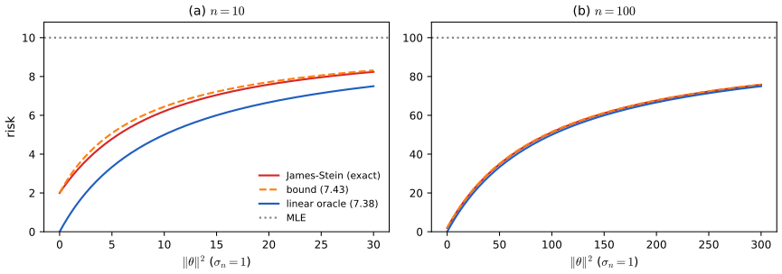
fig_7_S3, js_risk, js_bound, oracle_linear. Supplementary figure. Download: PDF · SVGSee also (companion course): Stein's paradox and the James–Stein estimator, with its empirical Bayes interpretation, in Probability and Statistical Inference, and the James–Stein demonstration there.
7.7 Adaptive Estimation Over Sobolev Spaces
p. 158 Pinsker's estimator needs \(m\) and \(c\). Efromovich and Pinsker (1984) showed that one estimator can be asymptotically minimax over every \(\Theta(m,c)\) at once: it is adaptively asymptotically minimax. The idea is to split the coefficients into blocks and apply James–Stein in each block, so that the shrinkage factor is estimated locally in frequency.
The scheme of Cai, Low and Zhao (2000): let \([a]\) be the integer part, \(b=1+1/\log n\), and \(K_0\) an integer with \([b^{K_0}]\ge3\) and \([b^k]-[b^{k-1}]\ge3\) for \(k\ge K_0+1\). The blocks are \(B_0=\{Z_i:1\le i\le[b^{K_0}]\}\) and \(B_k=\{Z_i:[b^{k-1}]\lt i\le[b^k]\}\) for \(k\ge K_0+1\); apply James–Stein within each block, and set \(\hth_i=0\) for \(i>[b^{K_1}]\), \(K_1=[\log_b n]-1\). For \(n=1000\) this gives 29 blocks, the first of 19 coefficients and the last ending at index 862.
Theorem 7.50 (Cai, Low and Zhao 2000) p. 158
Let \(\Theta(m,c)=\{\theta:\sum_ia_i^2\theta_i^2\le c^2\}\) with \(a_1=1\), \(a_{2i}^2=a_{2i+1}^2=1+(2i\pi)^{2m}\) (the book writes \(a_{2i}=a_{2i+1}=1+(2i\pi)^{2m}\); these are the squares), and let \(R_n(m,c)\) be its minimax risk. For all \(m>0\), \(c>0\),
\[ \lim_{n\to\infty}\frac{\sup_{\theta\in\Theta(m,c)}R(\hth,\theta)}{R_n(m,c)}=1. \]Filling the gap 7.9: why blockwise James–Stein adapts p. 158
Within a block, James–Stein loses at most \(2\sn^2\) to the best constant weight on that block (Theorem 7.47), and Pinsker's weights are nearly constant on each block because the blocks are short on the scale of the taper. The total loss, \(2\sn^2\) times the number of blocks, is of smaller order than the minimax risk.
Argument
Let \(B_0,\dots,B_K\) be the blocks, \(L_k=|B_k|\), and \(\hth\) blockwise James–Stein. Apply Theorem 7.47 in each block (the blocks are independent): for every \(\theta\),
\[ R(\hth,\theta)\le\sum_k\Big[2\sn^2+\min_{w}\sum_{i\in B_k}\big((1-w)^2\theta_i^2+w^2\sn^2\big)\Big]+\sum_{i>[b^{K_1}]}\theta_i^2. \]Blockwise constant weights are almost as good as Pinsker's. Let \(w_i=(1-a_i/\mu)_+\) be Pinsker's weights and \(\bar w_k\) the best constant weight on \(B_k\). Because the block endpoints grow geometrically with ratio \(b=1+1/\log n\), the ratio \(a_{\max}/a_{\min}\) within a block is at most about \(b^m\to1\), so the \(w_i\) vary by a factor \(1+O(m/\log n)\) relative to \(1-w_i\) within a block (except in the single block containing the cut-off \(a_i=\mu\), whose contribution is of smaller order). Hence \(\sum_k\min_w(\cdots)\le(1+o(1))\sum_i\big((1-w_i)^2\theta_i^2+w_i^2\sn^2\big)\le(1+o(1))R_n^L\) uniformly over \(\Theta(m,c)\).
The price of adaptation. The number of blocks is about \(\log_b n=\log n/\log(1+1/\log n)\approx(\log n)^2\), so the James–Stein penalties add up to \(2\sn^2(\log n)^2=2\sigma^2(\log n)^2/n\), which is \(o(n^{-2m/(2m+1)})\) for every \(m>0\). The tail. Coefficients beyond \([b^{K_1}]\approx n/b^2\) contribute at most \(c^2/a^2_{n/b^2}=O(n^{-2m})\), again negligible. Since \(R_n\sim R_n^L\) (Theorem 7.36), the ratio tends to 1. The details, including the first block and blocks shorter than 3, are in Cai, Low and Zhao (2000). These \(o(\cdot)\) terms are slow: \((\log n)^2/n\) against \(n^{-2/3}\) for \(m=1\) is only small for very large \(n\), as Figure 7.S8 shows.
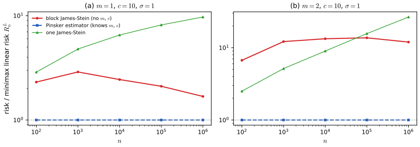
fig_7_S8, clz_blocks, block_js, block_js_study. Supplementary figure. Download: PDF · SVG7.8 Confidence Sets
pp. 159–166 A set \(B_n\subset\R^n\) is a \(1-\alpha\) confidence set if
\[ \inf_{\theta\in\R^n}\P_\theta(\theta\in B_n)\ge1-\alpha. \tag{7.51} \]Coverage must hold for every \(\theta\): this "honesty" is what makes small sets hard to build.
Method I: the \(\chi^2\) ball
Since \(\|Z-\theta\|^2/\sn^2\sim\chi^2_n\),
\[ B_n=\{\theta\in\R^n:\|Z-\theta\|^2\le\sn^2\chi^2_{n,\alpha}\} \tag{7.52} \]has coverage exactly \(1-\alpha\) for every \(\theta\), with \(\chi^2_{n,\alpha}\) the upper \(\alpha\) quantile. Its radius \(\sn\sqrt{\chi^2_{n,\alpha}}\approx\sn\sqrt n\) (the book's "expected radius \(n\sn^2\)" is the squared radius) is fixed; with \(\sn=\sigma/\sqrt n\) it does not shrink as \(n\to\infty\).
Improving the \(\chi^2\) ball by pre-testing
Test \(H_0:\theta=0\) with \(T_n=\sum_iZ_i^2\), rejecting when \(T_n>c_n^2\), \(\P(\chi^2_n>c_n^2/\sn^2)=\alpha/2\); by the Normal approximation \(c_n^2\approx\sn^2(n+\sqrt{2n}\,z_{\alpha/2})\). Let \(\varphi=1\) if the test rejects and set
\[ R_n=\begin{cases}B_n,&\varphi=1,\\\{\theta:\|\theta\|\le\Delta_n\},&\varphi=0,\end{cases}\qquad\Delta_n=\big(2\sqrt2\,z_{\alpha/2}\big)^{1/2}n^{1/4}\sn, \]with \(B_n\) the \(\chi^2\) ball at level \(\alpha/2\). If \(\theta=0\) or \(\|\theta\|\le\Delta_n\), the set fails only if \(\theta\notin B_n\), probability at most \(\alpha/2\). If \(\|\theta\|>\Delta_n\), it fails only if the test accepts (type II error) or \(\theta\notin B_n\): probability at most \(\beta(\theta)+\alpha/2\). So coverage is \(1-\alpha\) as long as the test has power at least \(1-\alpha/2\) beyond \(\Delta_n\). When the test accepts, the radius is \(\Delta_n\asymp\sn n^{1/4}\), far below \(\sn n^{1/2}\): a random-radius ball can be much smaller than the fixed one at some \(\theta\).
Filling the gap 7.10: the power of the pre-test, done carefully p. 160
The book's power calculation has a step with the inequality in the wrong direction. The conclusion is right to first order, and becomes exact if \(\Delta_n\) is enlarged slightly.
Derivation
Write \(Z_i=\theta_i+\sn\epsilon_i\). Then \(T_n=\|\theta\|^2+2\sn\sum\theta_i\epsilon_i+\sn^2\sum\epsilon_i^2\) has mean \(\|\theta\|^2+n\sn^2\) and variance \(4\sn^2\|\theta\|^2+2n\sn^4\) (the two random terms are uncorrelated because \(\E\epsilon^3=0\)). With \(u=\|\theta\|^2/(\sqrt n\sn^2)\) and the Normal approximation,
\[ \P_\theta(T_n>c_n^2)\approx\P\Big(N(0,1)>\frac{\sqrt2z_{\alpha/2}-u}{\sqrt{2+4u/\sqrt n}}\Big). \]The book bounds the threshold by replacing the denominator with \(\sqrt2\). When the numerator \(\sqrt2z_{\alpha/2}-u\) is negative (which is the relevant case), a larger denominator gives a threshold closer to zero, i.e. larger, so the probability is smaller, and the book's "\(\ge\)" goes the wrong way. The correct requirement for power \(\ge1-\alpha/2\) is \(\frac{u-\sqrt2z_{\alpha/2}}{\sqrt{2+4u/\sqrt n}}\ge z_{\alpha/2}\). As \(n\to\infty\) with \(u\) bounded the denominator tends to \(\sqrt2\), and the condition becomes \(u\ge2\sqrt2z_{\alpha/2}\), i.e. \(\|\theta\|\ge\Delta_n\): the book's \(\Delta_n\) is the right first-order answer. For finite \(n\) one needs \(u\) slightly larger: solving the quadratic, \(u\ge2\sqrt2z+4z^2/\sqrt n+O(1/n)\) with \(z=z_{\alpha/2}\). Numerically, with \(n=400\) and \(\alpha=0.05\), the exact power (noncentral \(\chi^2\)) at \(\|\theta\|=\Delta_n\) is 0.940, not the 0.975 needed; enlarging \(\Delta_n^2\) by the \(4z^2\sn^2\) term fixes it. The book also prints \(\|\theta\|^2n\sn^2\) for \(\|\theta\|^2+n\sn^2\) in the second line of the display.
Method II: Baraud's confidence set
Baraud (2004), building on Lepski (1999), generalises the pre-test to a family \(\mathcal S\) of linear subspaces of \(\R^n\), with \(\R^n\in\mathcal S\). For \(S\in\mathcal S\) let \(\Pi_S\) be the orthogonal projection, \(d(S)\) the dimension, \(e(S)=n-d(S)\), and
\[ B_S=\{\theta:\|\theta-\Pi_SZ\|\le\rho_S\}. \tag{7.53} \]Test whether \(\theta\) is close to \(S\) with \(\|Z-\Pi_SZ\|^2\), and use the smallest \(B_S\) among the subspaces not rejected. The radii are chosen so that
\[ \max_\theta\P_\theta\big(S\text{ is not rejected and }\theta\notin B_S\big)\le\alpha_S, \tag{7.54} \]with \(\sum_S\alpha_S\le\alpha\); a union bound then gives coverage \(1-\alpha\). Notation: \(\chi^2_{d,k}\) is noncentral chi-square with noncentrality \(d\) and \(k\) degrees of freedom, \(G_{d,k}\) its cdf, \(q_{d,k}(\alpha)=G_{d,k}^{-1}(1-\alpha)\) its upper \(\alpha\) quantile, and \(q_{d,k}(\alpha)=-\infty\) for \(\alpha\ge1\). Fix \(\alpha\in(0,1)\), \(\gamma\in(0,1-\alpha)\), and let
\[ \mathcal A=\Big\{S:\frac{\|Z-\Pi_SZ\|^2}{\sn^2}\le c(S)\Big\}, \tag{7.55} \] \[ c(S)=q_{0,e(S)}(\gamma), \tag{7.56} \]the subspaces not rejected by level-\(\gamma\) tests (\(\R^n\in\mathcal A\) always). The radii are
\[ \rho_S^2=\sn^2\times\begin{cases}\inf_{z>0}\{z:G_{z,n}(q_{0,n}(\gamma))\le\alpha_S\},&d(S)=0,\\[2pt]\sup_{z>0}\Big\{z+q_{0,d(S)}\Big(\dfrac{\alpha_S}{G_{z,e(S)}(c(S))}\Big)\Big\},&0\lt d(S)\lt n,\\[2pt]q_{0,n}(\alpha_S),&d(S)=n.\end{cases} \tag{7.57} \]Let \(\hat S=\argmin_{S\in\mathcal A}\rho_S\), \(\hth=\Pi_{\hat S}Z\), \(\hat\rho=\rho_{\hat S}\), and
\[ B_n=\{\theta\in\R^n:\|\hth-\theta\|^2\le\hat\rho^2\}. \tag{7.58} \]Theorem 7.59 (Baraud 2004) p. 163, (7.60)
\[ \inf_{\theta\in\R^n}\P_\theta(\theta\in B_n)\ge1-\alpha. \tag{7.60} \]Filling the gap 7.11: proof of Theorem 7.59, the two facts it uses, and Lemma 7.80 pp. 163–164, 169
The proof needs (i) that for a subspace \(S\) the two statistics in (7.61) are independent with explicit laws, by Pythagoras, and (ii) that the noncentral chi-square cdf decreases in the noncentrality. The book's proof misnames one statistic; here is the corrected version.
Proof
Reduction. \(\theta\notin B_n\) implies \(\theta\notin B_S\) for the selected \(S\in\mathcal A\), so
\[ \P_\theta(\theta\notin B_n)\le\sum_{S\in\mathcal S}a(S),\qquad a(S)=\P_\theta\big(\|\theta-\Pi_SZ\|>\rho_S,\ \|Z-\Pi_SZ\|^2\le\sn^2c(S)\big). \tag{7.61} \]It suffices to show \(a(S)\le\alpha_S\) for every \(\theta\).
Fact (i): Pythagoras. Write \(Z=\theta+\sn\epsilon\). Then \(\theta-\Pi_SZ=(\theta-\Pi_S\theta)-\sn\Pi_S\epsilon\), a sum of a vector orthogonal to \(S\) and a vector in \(S\), so
\[ \frac{\|\theta-\Pi_SZ\|^2}{\sn^2}=z+\|\Pi_S\epsilon\|^2=:A,\qquad z=\frac{\|\theta-\Pi_S\theta\|^2}{\sn^2}, \]with \(\|\Pi_S\epsilon\|^2\sim\chi^2_{d(S)}\). And \(Z-\Pi_SZ=(I-\Pi_S)\theta+\sn(I-\Pi_S)\epsilon\), so \(B:=\|Z-\Pi_SZ\|^2/\sn^2\sim\chi^2_{z,e(S)}\) (the book writes \(B=\|\theta-Z\|^2/\sn^2\), which is not the test statistic). Since \(\Pi_S\epsilon\) and \((I-\Pi_S)\epsilon\) are uncorrelated Gaussian vectors, \(A\) and \(B\) are independent.
Fact (ii): monotonicity. \(G_{z,k}(u)=\P(\chi^2_{z,k}\le u)\) is decreasing in \(z\). Indeed \(\chi^2_{z,k}\overset d=(\sqrt z+\xi)^2+\chi^2_{k-1}\) with independent pieces, and for fixed \(v\ge0\), \(\P((\sqrt z+\xi)^2\le v)=\P(\xi\in[-\sqrt v-\sqrt z,\sqrt v-\sqrt z])\), the probability that a standard Normal lies in an interval of fixed length whose centre \(-\sqrt z\) moves away from 0; by symmetry and unimodality of \(\phi\) this decreases in \(z\). Condition on \(\chi^2_{k-1}\).
Case \(0\lt d(S)\lt n\). By independence,
\[ a(S)=\P\Big(z+\chi^2_{d(S)}>\frac{\rho_S^2}{\sn^2}\Big)\,\P\big(\chi^2_{z,e(S)}\le c(S)\big)=\Big[1-G_{0,d(S)}\Big(\frac{\rho_S^2}{\sn^2}-z\Big)\Big]G_{z,e(S)}(c(S)). \tag{7.63} \]If \(G_{z,e(S)}(c(S))\le\alpha_S\) we are done. Otherwise the definition (7.57) gives \(\rho_S^2/\sn^2-z\ge q_{0,d(S)}(\alpha_S/G_{z,e(S)}(c(S)))\), and since \(1-G_{0,d}(q_{0,d}(p))=p\),
\[ 1-G_{0,d(S)}\Big(\frac{\rho_S^2}{\sn^2}-z\Big)\le\frac{\alpha_S}{G_{z,e(S)}(c(S))}, \tag{7.64} \]so \(a(S)\le\alpha_S\). Case \(d(S)=0\) (\(S=\{0\}\), \(\Pi_SZ=0\)): if \(\|\theta\|\le\rho_S\) then \(a(S)=0\); otherwise \(a(S)=\P(\|Z\|^2\le\sn^2q_{0,n}(\gamma))=G_{\|\theta\|^2/\sn^2,n}(q_{0,n}(\gamma))\le G_{\rho_S^2/\sn^2,n}(q_{0,n}(\gamma))\le\alpha_S\) by (ii) and the definition of \(\rho_S\). Case \(d(S)=n\): \(\|\theta-Z\|^2/\sn^2\sim\chi^2_n\), so \(a(S)\le\P(\chi^2_n>q_{0,n}(\alpha_S))=\alpha_S\).
The supremum in (7.57) is over a bounded range: once \(G_{z,e}(c(S))\le\alpha_S\) the quantile is \(-\infty\). In the code it is found by locating that endpoint with a root finder, scanning a grid and refining the maximiser; a direct simulation of \(a(S)\) for a 10-dimensional subspace at several \(z\) stays below \(\alpha_S\).
Lemma 7.80 (Section 7.9): if \(\theta\in S\) then \(z=0\) and \(\|Z-\Pi_SZ\|^2/\sn^2\sim\chi^2_{e(S)}\), so \(\P_\theta(S\in\mathcal A)=1-\gamma\) exactly; on that event \(\hat\rho\le\rho_S\). Hence \(\inf_{\theta\in S}\P_\theta(\hat\rho\le\rho_S)\ge1-\gamma\).
Unknown \(\sigma\). If \(\sn\) is only known to lie in \(I=[\sqrt{1-\eta_n}\tau_n,\tau_n]\), the radii become
\[ \rho_S^2=\begin{cases}\inf_{z>0}\{z:\sup_{\sn\in I}G_{z/\sn^2,n}(q_{0,n}(\gamma)\tau_n^2/\sn^2)\le\alpha_S\},&d(S)=0,\\\sup_{z>0,\sn\in I}\{z\sn^2+\sn^2q_{0,d(S)}(h_S(z,\sn))\},&0\lt d(S)\lt n,\\q_{0,n}(\alpha_S)\tau_n^2,&d(S)=n,\end{cases} \tag{7.65} \] \[ h_S(z,\sigma)=\frac{\alpha_S}{G_{z,e(S)}\big(q_{0,e(S)}(\gamma)\tau_n^2/\sigma^2\big)}, \tag{7.66} \] \[ \mathcal A=\{S\in\mathcal S:\|Z-\Pi_SZ\|^2\le q_{0,e(S)}(\gamma)\tau_n^2\}. \tag{7.67} \](The book's (7.66) has a doubled \(G_{z,e(S)}\); the version above is the one the proof of Theorem 7.59 needs.) The proof is the same, taking the worst \(\sn\in I\) at each step.
The Beran–Dümbgen–Stein pivotal method
Stein (1981), Li (1989), Beran and Dümbgen (1998) and Genovese and Wasserman (2005) use the nested subspaces \(S_j=\{\theta:\theta_{j+1}=\dots=\theta_n=0\}\), estimators \(\hth_m=(Z_1,\dots,Z_m,0,\dots,0)\), loss \(L_m=\|\hth_m-\theta\|^2\), SURE \(\hat R_m=m\sn^2+\sum_{j>m}(Z_j^2-\sn^2)\) and the pivot
\[ V_m=\sqrt n(L_m-\hat R_m). \tag{7.68} \]With \(\hat m\) minimising \(\hat R_m\), Beran and Dümbgen show \(V_{\hat m}/\hat\tau\rightsquigarrow N(0,1)\), where
\[ \tau_m^2=\V(V_m)=2n\sn^2\Big(n\sn^2+2\sum_{j>m}\theta_j^2\Big),\qquad \hat\tau^2=2n\sn^2\Big(n\sn^2+2\sum_{j>\hat m}(Z_j^2-\sn^2)\Big). \]The ball \(\{\theta:\|\hth_{\hat m}-\theta\|^2\le r_n^2\}\), \(r_n^2=\hat R_{\hat m}+\hat\tau z_\alpha/\sqrt n\), has asymptotic coverage \(1-\alpha\). Negative values of \(\sum_{j>\hat m}(Z_j^2-\sn^2)\) are replaced by 0, which can only enlarge the ball.
Filling the gap 7.12: the variance of the pivot p. 165
The formula for \(\tau_m^2\) is a two-line computation; it shows why the pivot has an \(n^{1/4}\)-scale radius.
Derivation
\(L_m=\sn^2\sum_{j\le m}\epsilon_j^2+\sum_{j>m}\theta_j^2\) and \(Z_j^2-\sn^2=\theta_j^2+2\sn\theta_j\epsilon_j+\sn^2(\epsilon_j^2-1)\), so
\[ L_m-\hat R_m=\sn^2\sum_{j\le m}(\epsilon_j^2-1)-\sum_{j>m}\big(2\sn\theta_j\epsilon_j+\sn^2(\epsilon_j^2-1)\big), \]a sum of independent mean-zero terms (\(\E L_m=\E\hat R_m\): SURE is unbiased). Using \(\V(\epsilon^2)=2\) and \(\cov(\epsilon,\epsilon^2)=0\), its variance is \(2m\sn^4+\sum_{j>m}(4\sn^2\theta_j^2+2\sn^4)=2n\sn^4+4\sn^2\sum_{j>m}\theta_j^2\). Multiplying by \(n\) gives \(\tau_m^2\). With \(\sn^2=\sigma^2/n\), \(\tau_m^2/n=O(1/n)\), so the radius correction \(\hat\tau z_\alpha/\sqrt n\) is \(O(\sn^2\sqrt n)\), and when \(\hat R_{\hat m}\) is small the squared radius is of order \(\sn^2\sqrt n\): radius of order \(\sn n^{1/4}\), the optimal order of Section 7.9. A simulation with \(n=30\) confirms the variance formula and the zero mean. The Normal limit for the data-chosen \(\hat m\) is the content of Beran and Dümbgen (1998); it is an approximation, and Table 7.1 and the demonstration show it can fail badly for a dense \(\theta\).
Example 7.69, Figure 7.2 and Table 7.1
p. 166 Nested subspaces \(S_0=\{0\},S_1,\dots,S_n\), \(\alpha=0.05\), \(n=100\), \(\sn=1/\sqrt n\), \(\alpha_S=\alpha/(n+1)\). Figure 7.2 shows \(\rho_S\) against \(d(S)\) for four values of \(\gamma\).
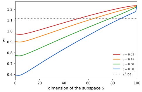
fig_7_2, baraud_kappa, baraud_table. Reproduces Wasserman (2006), Figure 7.2. Download: PDF · SVGLarge \(\gamma\) makes \(\rho_S\) small (the tests reject more easily, so the event "accepted and not covered" is rarer), but the true subspace is then rejected with probability \(\gamma\) (Lemma 7.80), and the ball falls back on a larger one. The book's sentence that large \(\gamma\) "increases the set \(\mathcal A\)" has the direction reversed: large \(\gamma\) shrinks \(\mathcal A\). The ratio \(\rho_0/\rho_n\) is of order \(n^{-1/4}\),
\[ \frac{\rho_0}{\rho_n}=O(n^{-1/4}), \tag{7.70} \]which is Exercise 12. The simulation uses \(\theta=(10,10,10,10,10,0,\dots,0)\) and 1000 data sets.
| Method | coverage | mean radius | book: coverage | book: radius |
|---|---|---|---|---|
| \(\chi^2\) | 0.955 | 1.115 | 0.950 | 1.115 |
| Baraud, \(\gamma=0.90\) | 0.996 | 1.062 | 1.000 | 0.973 |
| Baraud, \(\gamma=0.50\) | 1.000 | 0.898 | 1.000 | 0.904 |
| Baraud, \(\gamma=0.15\) | 1.000 | 0.922 | 1.000 | 0.779 |
| Baraud, \(\gamma=0.05\) | 1.000 | 0.974 | 0.996 | 0.605 |
| Pivotal | 1.000 | 0.585 | 0.998 | 0.582 |
The \(\chi^2\) and pivotal rows agree with the book. The Baraud rows do not, and cannot under the procedure as stated. With \(\sn=0.1\) the first five coordinates are 100 standard deviations from zero, so every \(S_d\) with \(d\lt 5\) is rejected and \(S_5\) is accepted with probability exactly \(1-\gamma\). The smallest possible radius is therefore about \(\min_{d\ge5}\rho_{S_d}\), namely 0.969, 0.899, 0.774 and 0.598 for \(\gamma=0.05,0.15,0.50,0.90\) (Figure 7.2). The book's four radii, 0.605, 0.779, 0.904 and 0.973 listed from \(\gamma=0.05\) to \(0.90\), are these minima in the reverse order of \(\gamma\), plus a little. So the book's table looks as if the \(\gamma\) labels were reversed and \(S_5\) were (almost) always accepted; with level-\(\gamma\) tests, \(S_5\) is rejected a fraction \(\gamma\) of the time and the mean radius grows, to 1.06 at \(\gamma=0.9\). Either way the conclusions of the example stand: the pivotal ball is about half the \(\chi^2\) ball, and Baraud's is in between.
See also: confidence balls and bands in general, Section 4.4 of these notes.
7.9 Optimality of Confidence Sets
pp. 166–170 How small can an honest ball be? If \(B_n\) has radius \(s_n\) then \(\E_\theta(s_n)\ge C_1\sn n^{1/4}\) for every \(\theta\) and \(\E_\theta(s_n)\ge C_2\sn n^{1/2}\) for some \(\theta\). The \(\chi^2\) ball has \(\sn n^{1/2}\) everywhere; Baraud's ball reaches \(\sn n^{1/4}\) at some points. Compare with estimation: the rate \(n^{-2m/(2m+1)}\) is achievable adaptively (Theorem 7.50), but a ball cannot adapt in the same way: without smoothness assumptions its radius is at least of order \(\sn n^{1/4}=O(n^{-1/4})\) when \(\sn=\sigma/\sqrt n\), and only limited adaptivity is possible (Robins and van der Vaart 2005; Juditsky and Lambert-Lacroix 2003; Cai and Low 2005).
Theorem 7.71 (Li 1989) p. 168, (7.72)–(7.73)
Let \(B_n=\{\theta^n:\|\hth^n-\theta^n\|\le s_n\}\), with any estimator \(\hth^n\) and radius \(s_n=s_n(Z^n)\), satisfy
\[ \liminf_{n\to\infty}\inf_{\theta^n\in\R^n}\P_{\theta^n}(\theta^n\in B_n)\ge1-\alpha. \tag{7.72} \]Then for any sequence \(\theta^n\) and any \(c_n\to0\),
\[ \limsup_{n\to\infty}\P_{\theta^n}(s_n\le c_n\sn n^{1/4})\le\alpha. \tag{7.73} \]Theorem 7.74 (Cai and Low) p. 168, (7.75)–(7.76)
In model (7.1), fix \(0\lt \alpha\lt 1/2\) and let \(B_n=\{\theta:\|\hth-\theta\|\le s_n\}\) satisfy \(\inf_\theta\P_\theta(\theta\in B_n)\ge1-\alpha\). For every \(0\lt \epsilon\lt 1/2-\alpha\),
\[ \inf_{\theta\in\R^n}\E_\theta(s_n)\ge\tfrac12\,\sn(1-2\alpha-2\epsilon)\,n^{1/4}\big(\log(1+\epsilon^2)\big)^{1/4}. \tag{7.75} \](The book's (7.75) has no factor \(\tfrac12\); the argument in its appendix only gives the bound with \(\tfrac12\), see Filling the gap 7.13.) With \(\sn=\sigma/\sqrt n\), \(\inf_\theta\E_\theta(s_n)\ge C/n^{1/4}\), \(C=\tfrac12\sigma(1-2\alpha-2\epsilon)(\log(1+\epsilon^2))^{1/4}\), the bound (7.76).
Filling the gap 7.13: proof of Theorem 7.74 (and Li's theorem) pp. 176–179
The idea is a two-point test in disguise: the point \(0\) and a uniform mixture over the \(2^n\) vertices of a small cube are statistically almost indistinguishable, so an honest ball must contain both with high probability, which forces its radius to be at least half their distance.
Proof
Let \(a=\sn n^{-1/4}(\log(1+\epsilon^2))^{1/4}\), \(\Omega=\{\theta:|\theta_i|=a,\ i=1,\dots,n\}\) (\(2^n\) points), \(f_\theta\) the \(N(\theta,\sn^2I)\) density and \(q=2^{-n}\sum_{\theta\in\Omega}f_\theta\).
Step 1: \(q\) is close to \(f_0\) in \(L_1\). By Cauchy–Schwarz,
\[ \int|f_0-q|=\int\frac{|f_0-q|}{\sqrt{f_0}}\sqrt{f_0}\le\Big(\int\frac{(f_0-q)^2}{f_0}\Big)^{1/2}=\Big(\int\frac{q^2}{f_0}-1\Big)^{1/2}. \](The book's display drops the square root and writes \(g\) for \(q\).) Expanding the square,
\[ \int\frac{q^2}{f_0}=\frac{1}{4^n}\sum_{\theta,\nu\in\Omega}\E_0\Big[\frac{f_\theta f_\nu}{f_0^2}(X)\Big],\qquad \frac{f_\theta f_\nu}{f_0^2}(x)=\exp\Big(\frac{x^\T(\theta+\nu)}{\sn^2}-\frac{\|\theta\|^2+\|\nu\|^2}{2\sn^2}\Big). \]Under \(f_0\), \(\E_0e^{x^\T v/\sn^2}=e^{\|v\|^2/(2\sn^2)}\), so each term equals \(\exp(\theta^\T\nu/\sn^2)\). Averaging over independent uniform \(\theta,\nu\in\Omega\), \(\theta_i\nu_i=a^2E_i\) with \(E_i=\pm1\) independent fair signs, so
\[ \int\frac{q^2}{f_0}=\prod_{i=1}^n\E e^{a^2E_i/\sn^2}=\cosh\Big(\frac{a^2}{\sn^2}\Big)^n\le\exp\Big(\frac{na^4}{2\sn^4}\Big)\le\exp\Big(\frac{na^4}{\sn^4}\Big)=1+\epsilon^2, \]using \(\cosh y\le e^{y^2/2}\) (compare the Taylor series term by term: \(y^{2k}/(2k)!\le y^{2k}/(2^kk!)\)) and \(na^4/\sn^4=\log(1+\epsilon^2)\). Hence \(\int|f_0-q|\le\epsilon\), and for every event \(A\), \(|Q(A)-P_0(A)|\le\epsilon\) (the book's (7.95)).
Step 2: two events. Let \(A=\{0\in B_n\}\) and \(B=\{\Omega\cap B_n\ne\emptyset\}\). Honest coverage gives \(P_0(A)\ge1-\alpha\) and \(P_\theta(B)\ge P_\theta(\theta\in B_n)\ge1-\alpha\) for each \(\theta\in\Omega\), hence \(Q(B)\ge1-\alpha\). Then
\[ P_0(A\cap B)\ge Q(A\cap B)-\epsilon\ge Q(A)+Q(B)-1-\epsilon\ge(P_0(A)-\epsilon)+(1-\alpha)-1-\epsilon\ge1-2\alpha-2\epsilon. \]Step 3: geometry. On \(A\cap B\) the ball contains \(0\) and some \(\theta\in\Omega\), with \(\|\theta\|=\sqrt na=\sn n^{1/4}(\log(1+\epsilon^2))^{1/4}=:c_n\). Both are within \(s_n\) of the centre \(\hth\), so \(c_n=\|\theta-0\|\le2s_n\): \(A\cap B\subseteq\{s_n\ge c_n/2\}\). (The book writes \(\{s_n\ge c_n\}\), which would need the centre to be one of the two points.) By Markov's inequality, \(\E_0s_n\ge\frac{c_n}2P_0(s_n\ge c_n/2)\ge\frac{c_n}2(1-2\alpha-2\epsilon)\). The same argument with \(\Omega\) translated to \(\theta_0+\Omega\) gives the bound at every \(\theta_0\), because the model is translation invariant. This proves (7.75) with the factor \(\tfrac12\).
Li's theorem 7.71 is the asymptotic form of the same argument: if \(\P_{\theta^n}(s_n\le c_n\sn n^{1/4})\) stayed above \(\alpha+\eta\), take \(a=\kappa\sn n^{-1/4}\) with \(\kappa\) so small that \(\int|f_{\theta^n}-q|\le\eta/2\) (around \(\theta^n\)); the ball must then contain points at distance \(\kappa\sn n^{1/4}\gg c_n\sn n^{1/4}\) with probability bounded away from zero, a contradiction.
Theorem 7.77 (Cai and Low) p. 169, (7.78)–(7.79)
Under the same assumptions, for every \(0\lt \epsilon\lt \tfrac12(\tfrac12-\alpha)\) (so that \(z_{\alpha+2\epsilon}>0\); the book's range \(\epsilon\lt \tfrac12-\alpha\) includes values where the bound is negative and empty),
\[ \sup_{\theta\in\R^n}\E_\theta(s_n)\ge\epsilon\,\sn z_{\alpha+2\epsilon}\sqrt n\sqrt{\frac{\epsilon}{1-\alpha-\epsilon}}. \tag{7.78} \]With \(\sn=\sigma/\sqrt n\), \(\sup_\theta\E_\theta(s_n)\ge C\), a constant: somewhere the radius cannot shrink at all (7.79).
Filling the gap 7.14: proof of Theorem 7.77 pp. 179–180
A Bayes argument with a counting loss shows that some \(\theta\) forces a constant fraction of coordinates to be missed by \(a=\sn z_{\alpha+2\epsilon}\); honesty then forces the radius to cover that error.
Proof
A counting loss. Let \(a=\sn z_{\alpha+2\epsilon}\), \(\Omega=\{\theta:|\theta_i|=a\}\), \(\pi\) uniform on \(\Omega\), and \(L(\hth,\theta)=\sum_i\I(|\hth_i-\theta_i|\ge a)\). The posterior factorises, \(\P(\theta_i=a\given y_i)=e^{2ay_i/\sn^2}/(1+e^{2ay_i/\sn^2})\), and the posterior expected loss \(\sum_i\P(|\hth_i-\theta_i|\ge a\given y_i)\) is minimised by \(\hth_i=a\,\sign(y_i)\) (any value at distance \(\lt a\) from one support point is at distance \(\ge a\) from the other, so the best choice is the more probable point). This rule errs on coordinate \(i\) exactly when \(y_i\) has the wrong sign, probability \(\Phi(-a/\sn)=\alpha+2\epsilon\), for every \(\theta\in\Omega\), so its Bayes risk is \(n(\alpha+2\epsilon)\). For any estimator \(\hth\), the maximum of \(\E_\theta L\) over the finite set \(\Omega\) is at least its \(\pi\)-average, which is at least the Bayes risk: \(\max_{\theta\in\Omega}\E_\theta L\ge n(\alpha+2\epsilon)\). (The book phrases this through "a constant-risk Bayes rule is minimax", Theorem 12.11 of the companion course; the averaging argument is all that is needed.)
From expectation to probability. Let \(\gamma=\epsilon/(1-\alpha-\epsilon)\), take \(\theta\in\Omega\) attaining the maximum, and let \(p=\P_\theta(L\ge\gamma n)\). Since \(L\le n\) always and \(L\lt \gamma n\) off that event, \(n(\alpha+2\epsilon)\le\E_\theta L\le\gamma n(1-p)+np\), so \(p\ge(\alpha+2\epsilon-\gamma)/(1-\gamma)=\alpha+\epsilon\), the last equality being direct algebra with the chosen \(\gamma\).
From the loss to the radius. If \(L\ge\gamma n\) then at least \(\gamma n\) coordinates are off by \(a\) or more, so \(\|\hth-\theta\|^2\ge\gamma na^2\). At the same \(\theta\), coverage gives \(\P_\theta(s_n^2\ge\|\hth-\theta\|^2)\ge1-\alpha\), so
\[ \P_\theta(s_n^2\ge\gamma na^2)\ge\P_\theta(s_n^2\ge\|\hth-\theta\|^2\ge\gamma na^2)\ge(1-\alpha)+(\alpha+\epsilon)-1=\epsilon. \](The book writes this with suprema on both sides, which is only valid because the same \(\theta\) is used.) Markov's inequality gives \(\E_\theta s_n\ge\epsilon a\sqrt{\gamma n}\), which is (7.78).
The lower bound of Theorem 7.74 (order \(\sn n^{1/4}\)) is smaller than that of Theorem 7.77 (order \(\sn n^{1/2}\)), which leaves room for adaptation: a ball can be small at some \(\theta\) as long as it is large elsewhere. Baraud's ball does this.
Lemma 7.80 p. 169, (7.81)
With \(\mathcal S,\alpha,\gamma,(\rho_S)\) as in Theorem 7.59, for each \(S\in\mathcal S\),
\[ \inf_{\theta\in S}\P_\theta(\hat\rho\le\rho_S)\ge1-\gamma. \tag{7.81} \]Proof at the end of Filling the gap 7.11.
Theorems 7.82 and 7.85 (Baraud 2004: the radii are essentially optimal) p. 170, (7.83)–(7.87)
Lower bound (7.82). Let \(B=\{\theta:\|\hth-\theta\|^2\le r^2\}\) be a \(1-\alpha\) ball, \(2\alpha+\gamma\lt 1-e^{-1/36}\), \(d(S)\le n/2\), and suppose
\[ \inf_{\theta\in S}\P_\theta(r\le r_S)\ge1-\gamma. \tag{7.83} \]Then for some \(C=C(\alpha,\gamma)>0\),
\[ r_S^2\ge C\sn^2\max\{d(S),\sqrt n\}. \tag{7.84} \]Upper bound (7.85). If \(d(S)\le n/2\) for every \(S\ne\R^n\), there is a universal \(C\) with
\[ \rho_S^2\le C\sn^2\max\{d(S),\sqrt{n\log(1/\alpha_S)},\log(1/\alpha_S)\}. \tag{7.86} \]With \(\sn\) only known to lie in \([\sqrt{1-\eta_n}\tau_n,\tau_n]\), the lower bound becomes
\[ r_S^2\ge C\tau_n^2\max\{\eta_nn/2,\ d(S)(1-\eta_n),\ \sqrt{n-d(S)}(1-\eta_n)\}, \tag{7.87} \]so knowing \(\sigma^2\) to within \(\eta_n=O(n^{-1/2})\) is needed to keep the \(\max\{\sqrt n,d(S)\}\) order.
Filling the gap 7.15: what Theorems 7.82 and 7.85 say, and where the terms come from p. 170
These are research results (Baraud 2004); here is how each term arises.
Explanation
The \(\sqrt n\) term in (7.84) is Theorem 7.74 again: inside any subspace, including \(\{0\}\), the mixture argument of Filling the gap 7.13 forces a radius of order \(\sn n^{1/4}\), i.e. \(r_S^2\gtrsim\sn^2\sqrt n\). The \(d(S)\) term: if \(\theta\) ranges over all of a \(d\)-dimensional subspace, the ball must cover a \(d\)-dimensional Normal mean, which needs squared radius of order \(d\sn^2\) (the \(\chi^2_d\) ball is optimal there). Taking \(S\) a single point recovers Theorem 7.74; taking \(S=\R^n\) recovers Theorem 7.77. The upper bound (7.86) follows from (7.57) with the Normal approximation of Exercise 12: the quantile \(q_{0,d}(\alpha_S/G)\) is \(d+O(\sqrt{d\log(1/\alpha_S)}+\log(1/\alpha_S))\), and the supremum over \(z\) is reached where the test with \(e(S)\) degrees of freedom starts to have power, \(z\asymp\sqrt{e(S)\log(1/\alpha_S)}\). With \(\alpha_S=\alpha/(n+1)\) for nested subspaces, the price for searching over \(n+1\) models is only a \(\sqrt{\log n}\) factor in the \(\sqrt n\) term. (7.87): an error \(\eta_n\) in \(\sigma^2\) shifts \(\|Z-\Pi_SZ\|^2\) by about \(\eta_n(n-d)\sn^2\), which a test cannot distinguish from signal; so the ball must allow for it.
7.10 Random Radius Bands?
pp. 170–171 For bands (sup-norm balls) the answer is no: Low (1997) shows, for estimating a density at a point, that any confidence interval valid over a smoothness class must have expected length, at every function in the class, at least of the order of the fixed-length minimax interval; the same holds for regression and for bands. The reason is that a sup-norm error is driven by one coordinate (one location), and a single Normal mean admits no adaptation: the two-point argument of Filling the gap 7.13, applied to one coordinate instead of a cube, gives a constant lower bound with no gain from averaging. For \(L_p\) balls,
\[ \|\theta\|_p=\begin{cases}\big(\sum_i|\theta_i|^p\big)^{1/p},&p\lt \infty,\\\max_i|\theta_i|,&p=\infty,\end{cases} \]the cases \(2\lt p\lt \infty\) are intermediate: some adaptivity, less than for \(L_2\). Testing has the same structure (Ingster and Suslina 2003). Exercise 9 builds the exact sup-norm ball around \(Z\).
7.11 Penalization, Oracles and Sparsity
pp. 171–172 Minimising \(\sum_i(Z_i-\theta_i)^2\) gives the MLE \(Z\). Adding a penalty gives the other estimators of this chapter.
Theorem 7.88 (penalised least squares) p. 171
Let \(J:\R^n\to[0,\infty)\), \(\lambda\ge0\), and let \(\hth\) minimise \(M=\sum_{i=1}^n(Z_i-\theta_i)^2+\lambda J(\theta)\). Then:
- \(\lambda=0\): \(\hth=Z\);
- \(J(\theta)=\sum\theta_i^2\): \(\hth_i=Z_i/(1+\lambda)\), linear shrinkage;
- \(J(\theta)=\sum|\theta_i|\): \(\hth_i=\sign(Z_i)(|Z_i|-\lambda/2)_+\), soft thresholding at \(\lambda/2\);
- \(J(\theta)=\#\{i:\theta_i\ne0\}\): \(\hth_i=Z_i\I(|Z_i|>\sqrt\lambda)\), hard thresholding at \(\sqrt\lambda\).
The book states the threshold as \(\lambda\) in both thresholding cases; with its normalisation of \(M\) the thresholds are \(\lambda/2\) and \(\sqrt\lambda\) (Filling the gap 7.16). Soft thresholding at \(\lambda\) is obtained with the penalty \(2\lambda\sum|\theta_i|\).
Filling the gap 7.16: proof of Theorem 7.88 p. 171
All four penalties are sums over coordinates, so \(M\) separates and each coordinate is a one-dimensional problem.
Proof
Write \(m(t)=(z-t)^2+\lambda j(t)\) for one coordinate.
Ridge, \(j(t)=t^2\): \(m'(t)=-2(z-t)+2\lambda t=0\) gives \(t=z/(1+\lambda)\); \(m\) is strictly convex.
Lasso, \(j(t)=|t|\): \(m\) is strictly convex, so \(t\) is the minimiser iff \(0\in\partial m(t)=\{-2(z-t)+\lambda s:s\in\partial|t|\}\). For \(t>0\) this reads \(t=z-\lambda/2\), valid iff \(z>\lambda/2\); for \(t\lt 0\), \(t=z+\lambda/2\), valid iff \(z\lt -\lambda/2\); \(t=0\) requires \(2z\in[-\lambda,\lambda]\), i.e. \(|z|\le\lambda/2\). Together, \(t=\sign(z)(|z|-\lambda/2)_+\). So the minimiser of (7.89) is the soft threshold at \(\lambda/2\), not at \(\lambda\).
\(L_0\), \(j(t)=\I(t\ne0)\): if \(t=0\) the cost is \(z^2\); if \(t\ne0\) the best choice is \(t=z\), with cost \(\lambda\). So \(t=z\) iff \(z^2>\lambda\): the hard threshold at \(\sqrt\lambda\).
A brute-force minimisation over a fine grid of \(t\), for 33 values of \(z\) and \(\lambda=1.4\), agrees with these three formulas.
The \(\ell_1\) criterion
\[ \sum_{i=1}^n(Z_i-\theta_i)^2+\lambda\sum_{i=1}^n|\theta_i| \tag{7.89} \]is the lasso (Tibshirani 1996) and basis pursuit (Chen, Donoho and Saunders 1998) in the orthonormal-design case; Chapter 9 uses soft thresholding for wavelets.
See also (companion course): ridge regression and the lasso in Statistical Learning: Theory and Methods, where the orthonormal-design formulas appear with the same factor of 2.
Oracles and sparsity. For one coordinate, estimating \(\theta_i\) by \(Z_i\) costs \(\sn^2\) and by 0 costs \(\theta_i^2\). An oracle that knows which is better has risk \(\min(\sn^2,\theta_i^2)\), and for the whole vector
\[ R_{\rm oracle}=\sum_{i=1}^n\min(\sn^2,\theta_i^2). \]Theorem 7.90 (Donoho and Johnstone 1994) p. 172, (7.91)
Let \(\lambda=\sn\sqrt{2\log n}\) and \(\hth_\lambda\) the soft threshold. For every \(\theta\in\R^n\), \(n\ge2\),
\[ \E_\theta\|\hth_\lambda-\theta\|^2\le(2\log n+1)(\sn^2+R_{\rm oracle}). \]No estimator does substantially better: as \(n\to\infty\),
\[ \inf_{\hth}\sup_{\theta\in\R^n}\frac{\E_\theta\|\hth-\theta\|^2}{\sn^2+R_{\rm oracle}}\sim2\log n. \tag{7.91} \]Filling the gap 7.17: proof of the oracle inequality p. 172
Three one-dimensional facts about the soft-threshold risk \(r(\lambda,\theta)\) (with \(\sn=1\)) give the bound: it is at most \(1+\lambda^2\); it grows by at most \(\theta^2\) from its value at 0; and at 0 it is tiny when \(\lambda=\sqrt{2\log n}\).
Proof
By scaling, take \(\sn=1\) and let \(r(\lambda,\theta)=\E(\hth(\theta+\epsilon)-\theta)^2\) for one coordinate; the full risk is \(\sum_ir(\lambda,\theta_i)\).
(a) \(r\le1+\lambda^2\). By (7.22), \(r=\E[1-2\I(|Z|\le\lambda)+\min(Z^2,\lambda^2)]\le1+\lambda^2\).
(b) \(r(\lambda,\theta)\le r(\lambda,0)+\theta^2\). The soft threshold \(s\) is 1-Lipschitz, so we may differentiate under the expectation: \(\partial_\theta r=2\E[(s(\theta+\epsilon)-\theta)(s'(\theta+\epsilon)-1)]\). Since \(s'-1=-\I(|\theta+\epsilon|\le\lambda)\) and \(s=0\) on that event, \(\partial_\theta r=2\theta\,\P(|\theta+\epsilon|\le\lambda)\in[0,2\theta]\) for \(\theta\ge0\). Integrating, \(r(\lambda,\theta)-r(\lambda,0)\le\theta^2\); \(r\) is even in \(\theta\).
(c) \(r(\lambda,0)\le4\phi(\lambda)/\lambda^3\). At \(\theta=0\) the error is \((|\epsilon|-\lambda)_+\), so \(r(\lambda,0)=2\int_0^\infty u^2\phi(\lambda+u)\d u\le2\phi(\lambda)\int_0^\infty u^2e^{-\lambda u}\d u=4\phi(\lambda)/\lambda^3\), using \(\phi(\lambda+u)=\phi(\lambda)e^{-\lambda u-u^2/2}\le\phi(\lambda)e^{-\lambda u}\). With \(\lambda=\sqrt{2\log n}\), \(\phi(\lambda)=1/(n\sqrt{2\pi})\), and \(4/(\sqrt{2\pi}\lambda^3)\le1\) as soon as \(\lambda\ge1.17\), true for every \(n\ge2\). So \(r(\lambda,0)\le1/n\).
Combine. By (a) and (b), \(r\le\min(r(\lambda,0)+\theta^2,1+\lambda^2)\le r(\lambda,0)+\min(\theta^2,1+\lambda^2)\le\frac1n+(1+\lambda^2)\min(\theta^2,1)\le(1+\lambda^2)\big(\frac1n+\min(\theta^2,1)\big)\). Summing over \(i\), and restoring \(\sn\), \(\E\|\hth_\lambda-\theta\|^2\le(2\log n+1)(\sn^2+\sum_i\min(\theta_i^2,\sn^2))\). Figure 7.S5(a) computes the worst-case ratio exactly: it never exceeds \(2\log n+1\) and approaches it for large \(n\).
The lower bound (7.91) (Donoho and Johnstone 1994) uses sparse two-point priors: independently, \(\theta_i=\mu_n\) with probability \(\varepsilon_n\) and \(0\) otherwise, with \(\mu_n\approx\sn\sqrt{2\log(1/\varepsilon_n)}\), at the boundary where a nonzero coordinate can just not be detected. Under this prior the oracle risk is about \(n\varepsilon_n\sn^2\) (each nonzero coordinate costs \(\min(\mu_n^2,\sn^2)=\sn^2\)), while the Bayes risk is about \(n\varepsilon_n\mu_n^2\approx n\varepsilon_n\sn^2\cdot2\log(1/\varepsilon_n)\), because no rule can separate the rare nonzero coordinates from the noise. Taking for example \(\varepsilon_n=(\log n)/n\), so that \(n\varepsilon_n\to\infty\) and \(\log(1/\varepsilon_n)\sim\log n\), the ratio is \(\sim2\log n\), and a Bayes risk bounds the minimax risk from below.
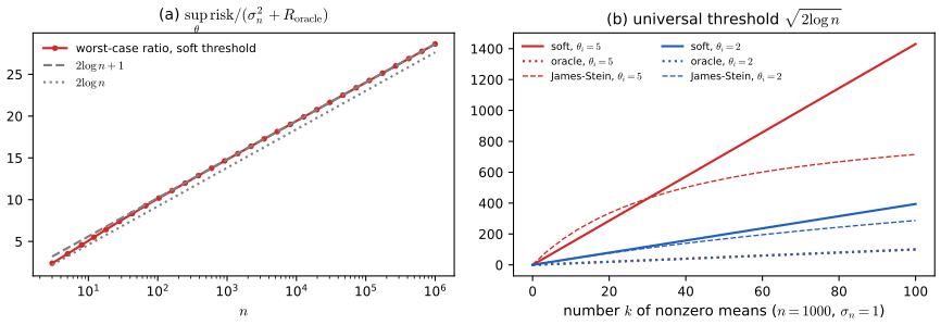
fig_7_S5, dj_ratio. Supplementary figure. Download: PDF · SVGIf \(\theta\) is zero except for \(k\ll n\) large components, \(R_{\rm oracle}=k\sn^2\); with \(\sn^2=O(1/n)\) in function estimation, this is \(O(k/n)\), small when \(k\) is small, and thresholding achieves it up to \(2\log n\).
7.12 Bibliographic Remarks
p. 172 Reducing nonparametric problems to Normal means (or white noise) goes back at least to Ibragimov and Has'minskii (1977) and Efromovich and Pinsker (1982); asymptotic equivalence was made precise by Brown and Low (1996) and Nussbaum (1996a). Johnstone's monograph (cited by the book as Johnstone 2003) treats Gaussian decision theory and its relation to nonparametric problems in depth; for hypothesis testing in this framework see Ingster and Suslina (2003).
7.13 Appendix
The white noise model
p. 173 A standard Brownian motion \(W(t)\), \(0\le t\le1\), has \(W(0)=0\), increments \(W(s+t)-W(s)\sim N(0,t)\), and independent increments over disjoint intervals. With \(Z_i=f(i/n)+\sigma\epsilon_i\), let
\[ Z_n(t)=\frac1n\sum_{i=1}^{[nt]}Z_i=\frac1n\sum_{i=1}^{[nt]}f(i/n)+\frac{\sigma}{\sqrt n}\cdot\frac1{\sqrt n}\sum_{i=1}^{[nt]}\epsilon_i \](the book writes \(Z_i\) in the last sum, where it means \(\epsilon_i\)). The first term tends to \(\int_0^tf\) and the normalised partial sums of the noise tend to Brownian motion (for one \(t\) this is the central limit theorem; as a process, Donsker's theorem). This suggests
\[ \d Z(t)=f(t)\,\d t+\frac{\sigma}{\sqrt n}\,\d W(t), \tag{7.92} \]the white noise model. Projecting on an orthonormal basis, \(Z_i=\int\phi_i\,\d Z=\theta_i+(\sigma/\sqrt n)\epsilon_i\) with \(\epsilon_i=\int\phi_i\,\d W\).
Filling the gap 7.18: why \(\int\phi_i\,\d W\) are iid \(N(0,1)\), and weak derivatives pp. 173–174
The stochastic integral of a deterministic function against Brownian motion is Gaussian with variance \(\int\phi^2\) (the Wiener isometry); orthonormal functions give independent coordinates.
Derivation
Wiener integral. For a step function \(\phi=\sum_kc_k\I_{(t_{k-1},t_k]}\) define \(\int\phi\,\d W=\sum_kc_k(W(t_k)-W(t_{k-1}))\): a sum of independent Normals, so Gaussian with mean 0 and variance \(\sum_kc_k^2(t_k-t_{k-1})=\int\phi^2\). The map \(\phi\mapsto\int\phi\,\d W\) is therefore an isometry from step functions in \(L_2(0,1)\) to \(L_2(\P)\), and extends uniquely to all of \(L_2(0,1)\); limits of Gaussian variables in \(L_2\) are Gaussian. By polarisation, \(\cov(\int\phi\,\d W,\int\psi\,\d W)=\int\phi\psi\), and any finite collection of such integrals is jointly Gaussian. For orthonormal \(\phi_i\) the \(\epsilon_i=\int\phi_i\,\d W\) are jointly Gaussian with identity covariance, hence iid \(N(0,1)\). Then \(\int\phi_i\,\d Z=\int\phi_if+\frac{\sigma}{\sqrt n}\epsilon_i=\theta_i+\frac{\sigma}{\sqrt n}\epsilon_i\): the sequence model (7.2), exactly.
Weak differentiability. \(f\), integrable on bounded intervals, is weakly differentiable if there is \(f'\), integrable on bounded intervals, with \(\int_x^yf'(s)\d s=f(y)-f(x)\) for \(x\le y\); equivalently \(\int f\varphi'=-\int f'\varphi\) for every smooth compactly supported \(\varphi\) (Härdle et al. 1998). The first form shows that a weakly differentiable function is continuous (absolutely continuous), which is why the hard threshold (7.23), which jumps at \(\pm\lambda\), is not (Exercise 6). For a vector function \(g:\R^n\to\R^n\), Theorem 7.17 needs each \(g_i\) to be weakly differentiable in each coordinate, i.e. absolutely continuous along almost every line parallel to the axes, with integrable partial derivatives.
Proofs of Theorems 7.28, 7.74 and 7.77
pp. 174–180 The book's appendix proves Pinsker's Theorem 7.28 (following Nussbaum 1996b) and Theorems 7.74 and 7.77. These notes give the complete proofs where the theorems are stated: Filling the gap 7.4 (Theorem 7.28, with the projection step that the book's "taking the infimum over estimators with values in \(\Theta_n\)" needs, and the chi-square deviation inequality \(\P(|n^{-1}\sum(\xi_j^2-1)|>t)\le2e^{-nt^2/8}\)), Filling the gap 7.13 (Theorem 7.74, with the factor \(\tfrac12\)) and Filling the gap 7.14 (Theorem 7.77). The Bayes-estimator facts used there, that the posterior mean minimises the Bayes risk for squared error and \(\argmin_a\E[L(a,\theta)\given Z]\) in general, are standard (the companion course's Section 12.3). The book's (7.93) defines \(B(\pi_n)=\inf_{\hth}B(\hth,\pi_n)\), and in its computation of \(\E_{\pi_n}(\sum_j\theta_j^2)^2\) the cross term has \(n(n-1)\) pairs, not \(\binom n2\); the conclusion \(O(1)\) is unaffected.
7.14 Exercises
Exercise 7.1. Let \(\theta_i=1/i^2\), \(i=1,\dots,n=1000\), and \(Z_i\sim N(\theta_i,1)\). Compute the risk of the MLE and of \(bZ\) as a function of \(b\), and the optimal \(b_*\). Simulate the modified James–Stein factor \(\hat b=(1-n/\sum_iZ_i^2)_+\) and compare it with \(b_*\); compare the risks of the MLE and of James–Stein (by simulation) with the Pinsker bound.
Solution
Here \(\sn=1\). The MLE has risk \(n=1000\) (a simulation gives 996.9). By (7.37), \(R(bZ,\theta)=(1-b)^2\|\theta\|^2+1000b^2\) with \(\|\theta\|^2=\sum_{i\le1000}i^{-4}=1.08232\) (equal to \(\pi^4/90\) to eight digits). So \(b_*=1.08232/1001.08=0.001081\) and the oracle risk (7.38) is \(1.0812\). The Pinsker bound for the ball of radius \(c=\|\theta\|\) with \(n\sn^2=1000\) is the same number, \(n\sn^2c^2/(n\sn^2+c^2)=1.0812\). In 1000 simulations the James–Stein factor was exactly 0 in 51% of them (\(\sum Z_i^2\lt n\)) and averaged 0.016; its histogram (Figure 7.S6) is a spike at 0 with a tail to about 0.08, so \(\hat b\) is a noisy estimate of the tiny \(b_*\) but always small. The simulated risk of the positive-part estimator is \(1.90\pm0.06\), within the oracle inequality \(R\le2+1.08\); the plain estimator (7.41) has exact risk 3.08 by (7.44). Both are about 500 times better than the MLE. Code:
ex1,fig_7_S6.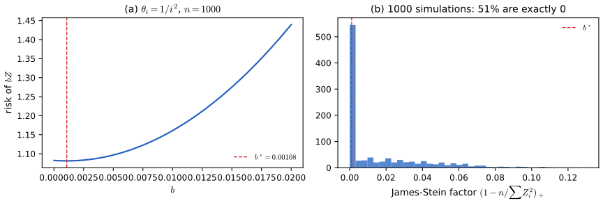
Figure 7.S6. Exercise 1: the risk of \(bZ\) against \(b\), and the simulated modified James–Stein factors. Code: fig_7_S6. Supplementary figure. Download: PDF · SVGExercise 7.2. The curved soft threshold \(\hth_i=-(Z_i+\lambda)^2\) for \(Z_i\lt -\lambda\), \(0\) for \(|Z_i|\le\lambda\), \((Z_i-\lambda)^2\) for \(Z_i>\lambda\). (a) Find its risk (hint: \(R=\E(\text{SURE})\)). (b) In the setting of Exercise 1, choose \(\lambda\) by SURE and compare with James–Stein; repeat for \(\theta=(10,\dots,10,0,\dots,0)\) with ten 10's and 990 zeros.
Solution
(a) With \(\sn=\sigma\), \(\hth_i=\sign(Z_i)(|Z_i|-\lambda)_+^2\) is continuous (it is 0 at \(\pm\lambda\)) and piecewise smooth, so weakly differentiable, with derivative \(2(|Z_i|-\lambda)_+\). Hence \(D_{ii}=2(|Z_i|-\lambda)_+-1\), and by (7.19)
\[ \sure=n\sigma^2+2\sigma^2\sum_i\big(2(|Z_i|-\lambda)_+-1\big)+\sum_ig_i^2,\qquad g_i=\sign(Z_i)(|Z_i|-\lambda)_+^2-Z_i. \]The risk is its expectation, \(\sum_ir(\theta_i)\) with \(r(\theta)=\E\big[-\sigma^2+4\sigma^2(|Z|-\lambda)_++g^2\big]\), \(Z\sim N(\theta,\sigma^2)\), an integral of polynomials against a Normal density over \(|z|>\lambda\), expressible with \(\Phi\) and \(\phi\) (the code evaluates it by quadrature, and a simulation confirms both the unbiasedness of SURE and the risk). (b) Averaging 200 simulations, with \(\lambda\) minimising SURE over a grid on \([0,12]\): for \(\theta_i=1/i^2\) the curved threshold has risk 2.77 against 2.07 for positive-part James–Stein (and 7.25 for soft thresholding with the SURE threshold); for ten 10's, 301 against 500 for James–Stein and 65 for SURE soft thresholding. The curved estimator squares the excess over \(\lambda\), which is not a sensible shape: for large means it needs \(\lambda\approx\theta-\sqrt\theta\) to be unbiased and then multiplies the noise by about \(2\sqrt\theta\). It beats James–Stein on the sparse vector only because James–Stein cannot exploit sparsity at all. Code:
curved_soft,sure_curved,risk_curved,ex2.Exercise 7.3. Let \(J=J_n\to\infty\) and \(\hat\sigma^2=\frac nJ\sum_{i=n-J+1}^nZ_i^2\), \(Z_i\sim N(\theta_i,\sigma^2/n)\). Show that \(\hat\sigma^2\) is uniformly consistent for \(\sigma^2\) over a Sobolev ellipsoid of order \(m>1/2\).
Solution
Assume also \(J\le n/2\) (the highest-frequency half; otherwise low-frequency signal enters the estimate and the claim fails). Since \(\E Z_i^2=\theta_i^2+\sigma^2/n\) and \(\V(Z_i^2)=2\sigma^4/n^2+4\theta_i^2\sigma^2/n\),
\[ \E\hat\sigma^2-\sigma^2=\frac nJ\sum_{i>n-J}\theta_i^2=:b_n(\theta),\qquad \V(\hat\sigma^2)=\frac{2\sigma^4}J+\frac{4\sigma^2}{J}b_n(\theta). \]On \(\Theta(m,c)\), \(\sum_{i>n-J}\theta_i^2\le c^2/a_{n-J}^2\le c^2/(\pi n/2-\pi)^{2m}\), so \(\sup_\theta b_n(\theta)\le\frac nJc^2(\pi(n/2-1))^{-2m}=O(n^{1-2m})\to0\) for \(m>1/2\) (already with \(J\ge1\)). Hence \(\sup_\theta\E(\hat\sigma^2-\sigma^2)^2=\sup(b_n^2+\V)\le O(n^{2-4m})+2\sigma^4/J+O(n^{1-2m}/J)\to0\), and Chebyshev gives \(\sup_\theta\P_\theta(|\hat\sigma^2-\sigma^2|>\varepsilon)\to0\) for every \(\varepsilon>0\).
Exercise 7.4. Prove Stein's lemma: if \(X\sim N(\mu,\sigma^2)\) then \(\E(g(X)(X-\mu))=\sigma^2\E g'(X)\).
Solution
See Filling the gap 7.3: write \((x-\mu)\varphi(x)=-\sigma^2\varphi'(x)\) and integrate by parts, in the form of Fubini's theorem applied to \(g(x)-g(\mu)=\int_\mu^xg'\), which needs only weak differentiability and \(\E|g'(X)|\lt \infty\). A quadrature check with \(g(t)=\sin t+t^3\), \(\mu=0.7\), \(\sigma=1.3\) gives the two sides equal to ten digits.
Exercise 7.5. Verify (7.22).
Solution
See the box after Example 7.20: \(g_i^2=\min(Z_i^2,\lambda^2)\) and \(D_{ii}=-\I(|Z_i|\le\lambda)\), substituted in (7.19). The closed form agrees with a finite-difference SURE (7.19) to six digits, and its average over 40000 simulated data sets agrees with the exact risk of Exercise 7.
Exercise 7.6. Show that the hard threshold estimator (7.23) is not weakly differentiable.
Solution
Let \(h(z)=z\I(|z|>\lambda)\). If \(h\) were weakly differentiable, \(h(y)-h(x)=\int_x^yh'(s)\d s\) with \(h'\) integrable near \(\lambda\), so \(h(y)-h(x)\to0\) as \(x\uparrow\lambda\), \(y\downarrow\lambda\) (absolute continuity of the integral). But \(h(x)=0\) for \(x\le\lambda\) and \(h(y)=y>\lambda\) for \(y>\lambda\), so the difference tends to \(\lambda\ne0\). Equivalently, the distributional derivative of \(h\) is \(\I(|z|>\lambda)+\lambda(\delta_\lambda+\delta_{-\lambda})\), which contains point masses and is not a function. Using (7.19) with \(D_{ii}=\I(|Z_i|>\lambda)-1\) ignores these masses and underestimates the risk by \(2\sigma\lambda\sum_i[\phi((\lambda-\theta_i)/\sigma)+\phi((\lambda+\theta_i)/\sigma)]\) in expectation (checked by numerical integration).
Exercise 7.7. Compute the risk functions of the soft threshold (7.21) and the hard threshold (7.23).
Solution
By scaling take \(\sigma=1\), one coordinate, \(Z=\theta+\epsilon\). Use \(\int_a^\infty x\phi=\phi(a)\) and \(\int_a^\infty x^2\phi=1-\Phi(a)+a\phi(a)\).
Hard threshold. The error is \(-\theta\) when \(|Z|\le\lambda\) and \(\epsilon\) otherwise. \(\P(|Z|\le\lambda)=\Phi(\lambda-\theta)-\Phi(-\lambda-\theta)\), and \(\E[\epsilon^2;\epsilon>\lambda-\theta]+\E[\epsilon^2;\epsilon\lt -\lambda-\theta]=[1-\Phi(\lambda-\theta)+(\lambda-\theta)\phi(\lambda-\theta)]+[\Phi(-\lambda-\theta)+(\lambda+\theta)\phi(\lambda+\theta)]\). So
\[ r_H(\lambda,\theta)=\theta^2[\Phi(\lambda-\theta)-\Phi(-\lambda-\theta)]+1-\Phi(\lambda-\theta)+\Phi(-\lambda-\theta)+(\lambda-\theta)\phi(\lambda-\theta)+(\lambda+\theta)\phi(\lambda+\theta). \]Soft threshold. By (7.22), \(r_S=\E[1-2\I(|Z|\le\lambda)+\min(Z^2,\lambda^2)]=1+\lambda^2-(2+\lambda^2)p+\E[Z^2;|Z|\le\lambda]\) with \(p=\P(|Z|\le\lambda)\). Computing \(\E[Z^2;|Z|\le\lambda]=\E[(\theta+\epsilon)^2;-\lambda-\theta\le\epsilon\le\lambda-\theta]\) with the two integrals above gives
\[ r_S(\lambda,\theta)=1+\lambda^2+(\theta^2-\lambda^2-1)[\Phi(\lambda-\theta)-\Phi(-\lambda-\theta)]-(\lambda-\theta)\phi(\lambda+\theta)-(\lambda+\theta)\phi(\lambda-\theta). \]Both formulas agree with numerical integration to ten digits. Figure 7.S2(a) plots them: \(r_S\) increases from \(r_S(\lambda,0)\) to \(1+\lambda^2\); \(r_H\) overshoots near \(\theta\approx\lambda\) (to about 2.5 when \(\lambda=2\)) and returns to 1 for large \(\theta\). With general \(\sigma\), \(r(\lambda,\theta;\sigma)=\sigma^2r(\lambda/\sigma,\theta/\sigma)\).
Exercise 7.8. Generate \(Z_i\sim N(\theta_i,1)\), \(i=1,\dots,100\), \(\theta_i=1/i\). Compute 95% balls by the \(\chi^2\), Baraud and pivotal methods; repeat 1000 times and compare the radii.
Solution
With \(\sn=1\), nested subspaces, \(\alpha_S=0.05/101\) and \(\gamma=0.5\): the \(\chi^2\) ball has radius \(\sqrt{124.34}=11.15\) and coverage 0.960; Baraud's ball has mean radius 8.93 and coverage 1.000; the pivotal ball has mean radius 5.46 and coverage 0.999. Only \(\theta_1=1\) is at the noise level, so low-dimensional subspaces are accepted; Baraud's radius is bimodal (about 7.7 when a small subspace is accepted, 10–12.4 otherwise), and the pivotal radius is concentrated near 5. Code:
ex8,fig_7_S7.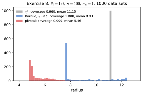
Figure 7.S7. Exercise 8: radii of the three confidence balls over 1000 simulated data sets, \(\theta_i=1/i\), \(n=100\), \(\sn=1\). Code: fig_7_S7. Supplementary figure. Download: PDF · SVGExercise 7.9. Construct \(B_n=\{\theta:\|\theta-Z\|_\infty\le c_n\}\) with \(\P_\theta(\theta\in B_n)\ge1-\alpha\) for all \(\theta\), under (7.1) with \(\sn=\sigma/\sqrt n\), and find its diameter.
Solution
\(\theta\in B_n\) iff \(\max_i|\epsilon_i|\le c_n/\sn\), which has probability \((2\Phi(c_n/\sn)-1)^n\), the same for every \(\theta\). Setting it to \(1-\alpha\):
\[ c_n=\frac{\sigma}{\sqrt n}\,\Phi^{-1}\Big(\frac{1+(1-\alpha)^{1/n}}2\Big). \](Bonferroni, \(c_n=\sn z_{\alpha/(2n)}\), is slightly conservative.) The sup-norm diameter is \(2c_n\) (deterministic). Since \(1-(1-\alpha)^{1/n}\approx-\log(1-\alpha)/n\), \(c_n/\sn\approx\sqrt{2\log n}\) and the diameter is \(\approx2\sigma\sqrt{2\log n/n}\). For \(\sigma=1\), \(\alpha=0.05\): \(c_{100}=0.347\), \(c_{1000}=0.128\). Each coordinate is pinned down to within \(O(\sqrt{\log n/n})\), but the \(L_2\) radius of this box is \(\sqrt n\,c_n\approx\sigma\sqrt{2\log n}\), larger than the \(\chi^2\) ball's \(\approx\sigma\): boxes and balls answer different questions.
Exercise 7.10. In Example 7.24 let \(\delta=\max_{S\in\mathcal S}\sup_\theta|\sure_S-R(\hth_S,\theta)|\). Bound \(\delta\) when (i) \(\mathcal S\) is a single model, (ii) nested models, (iii) all subsets.
Solution
With \(W_i=Z_i^2-\sn^2-\theta_i^2=2\sn\theta_i\epsilon_i+\sn^2(\epsilon_i^2-1)\), \(\sure_S-R(\hth_S,\theta)=\sum_{i\notin S}W_i\). As written, the supremum over \(\theta\in\R^n\) is infinite (the term \(2\sn\theta_i\epsilon_i\) is unbounded in \(\theta\)), so restrict to \(\|\theta\|\le c\) and bound \(\E\delta\). Note \(\E W_i=0\), \(\V(W_i)=4\sn^2\theta_i^2+2\sn^4\).
(i) One model: \(\E|\sum_{i\notin S}W_i|\le(\sum\V W_i)^{1/2}\le\sqrt{2n\sn^4+4\sn^2c^2}\), of order \(\sn^2\sqrt n+\sn c\). (ii) Nested: the tail sums \(T_m=\sum_{i>m}W_i\) form a martingale in reverse time, and Doob's \(L^2\) maximal inequality gives \(\E\max_m|T_m|\le2(\E T_0^2)^{1/2}\le2\sqrt{2n\sn^4+4\sn^2c^2}\): the same order as one model. (iii) All subsets: \(\max_S|\sum_{i\notin S}W_i|=\max(\sum_iW_i^+,\sum_iW_i^-)\ge\frac12\sum_i|W_i|\), which grows like \(n\): at \(\theta=0\), \(\E\sum_iW_i^+=n\sn^2\E(\epsilon^2-1)^+=2\phi(1)n\sn^2\approx0.48n\sn^2\). Simulation at \(\theta=0\), \(\sn=1\): \(\E\delta=11.0,\ 16.5,\ 54.0\) for (i), (ii), (iii) with \(n=100\), and \(21.7,\ 33.7,\ 204.5\) with \(n=400\): the first two double (\(\sqrt n\)), the last quadruples (\(n\)). So SURE is uniformly reliable over nested models but not over all subsets, where its minimum is biased downwards by order \(n\sn^2\), the size of the risk itself. Code:
ex10.Exercise 7.11. Find \(\mathrm{BIC}_B=\ell_B-\frac{|B|}2\log n\) explicitly in the Normal means model, and compare selection by maximising BIC with selection by minimising SURE: risk, and probability of selecting the true submodel.
Solution
For the submodel \(B\) (\(\theta_i=0\) for \(i\notin B\)) the MLE is \(\hth_B\) of (7.25) and \(\ell_B=-\frac1{2\sn^2}\sum_{i\notin B}Z_i^2+\const\). So \(\mathrm{BIC}_B=\const-\sum_{i\notin B}\frac{Z_i^2}{2\sn^2}-\frac{|B|}2\log n\), maximised by including \(i\) iff \(Z_i^2>\sn^2\log n\): hard thresholding at \(\sn\sqrt{\log n}\). Minimising SURE (7.26) (equivalently \(C_p\) or AIC) over all subsets includes \(i\) iff \(Z_i^2>2\sn^2\): hard thresholding at \(\sqrt2\sn\). Simulations with \(\sn=1\), \(k=10\) nonzero means of size \(\mu\), 500 data sets (risk; probability of exactly the true model; mean number of misclassified coordinates):
\(n\), \(\mu\) BIC risk BIC exact BIC errors SURE risk SURE exact SURE errors 100, 2 45.0 0.000 8.3 67.6 0.000 16.9 100, 5 28.5 0.068 2.8 61.5 0.000 14.2 1000, 2 107.7 0.000 15.8 579.5 0.000 157.8 1000, 5 84.8 0.000 8.5 572.9 0.000 155.0 SURE keeps every noise coordinate with \(|Z_i|>\sqrt2\), about 16% of them, and pays about \(0.16\cdot\E[\epsilon^2\given|\epsilon|>\sqrt2]\approx0.57\) per noise coordinate: for sparse vectors BIC wins on risk too. Neither finds the exact model reliably, because some of \(n-k\) noise coordinates always exceed the threshold; BIC is consistent for the model only in the limit (and slowly, since the false-positive rate per coordinate is \(\approx2\phi(\sqrt{\log n})/\sqrt{\log n}\), which times \(n\) grows like \(\sqrt{n/\log n}\)). For dense vectors with many moderate means, SURE's lower threshold has smaller risk: selecting the model and estimating \(\theta\) are different goals (Wasserman 2000). Code:
ex11,ex11_table.See also (companion course): BIC in Statistical Learning: Theory and Methods.
Exercise 7.12. Using a Normal approximation to the noncentral \(\chi^2\), approximate \(\rho_0\) and \(\rho_n\) in Example 7.69 and prove (7.70).
Solution
Approximate \(\chi^2_{z,k}\approx N(k+z,2k+4z)\) and \(q_{0,k}(p)\approx k+z_p\sqrt{2k}\). For \(d=n\): \(\rho_n^2/\sn^2=q_{0,n}(\alpha_S)\approx n+z_{\alpha_S}\sqrt{2n}\). For \(d=0\), the condition defining \(\rho_0\) becomes
\[ G_{z,n}(q_{0,n}(\gamma))\approx\Phi\Big(\frac{z_\gamma\sqrt{2n}-z}{\sqrt{2n+4z}}\Big)\le\alpha_S\iff z-z_\gamma\sqrt{2n}\ge z_{\alpha_S}\sqrt{2n+4z}. \]The solution has \(z=O(\sqrt n)\), so \(4z\ll2n\) and to leading order
\[ \frac{\rho_0^2}{\sn^2}\approx\sqrt{2n}\,(z_\gamma+z_{\alpha_S}),\qquad \frac{\rho_0}{\rho_n}\approx\Big(\frac{\sqrt{2n}(z_\gamma+z_{\alpha_S})}{n}\Big)^{1/2}=\Big(\frac2n\Big)^{1/4}(z_\gamma+z_{\alpha_S})^{1/2}. \]For fixed \(\alpha_S\) this is \(O(n^{-1/4})\), which is (7.70). With \(\alpha_S=\alpha/(n+1)\), \(z_{\alpha_S}\sim\sqrt{2\log n}\) and the ratio is \(O((\log n)^{1/4}n^{-1/4})\): (7.70) holds up to this logarithmic factor. Exact values (\(\gamma=0.5\)): \(\rho_0/\rho_n=0.626,\ 0.486,\ 0.367\) for \(n=100,400,1600\); times \(n^{1/4}\) this is \(1.98,\ 2.17,\ 2.32\), growing slowly as the \((\log n)^{1/4}\) factor predicts. For \(n=400\) the approximation \(\sqrt{2n}(z_\gamma+z_{\alpha_S})\) is within 25% of the exact \(\rho_0^2/\sn^2=120.8\) (the neglected \(4z\) term matters at this \(n\)), and \(n+z_{\alpha_S}\sqrt{2n}\) is within 3% of \(\rho_n^2/\sn^2=512.0\).
Notes on the book
Slips found while writing these notes, with the evidence. The book's website has no errata list.
Page 149, Theorem 7.11: the Fourier basis needs \(\sqrt2\), and \(a_j^2\sim(\pi j)^{2m}\)
The basis is printed as \(\phi_{2j}=\frac1{\sqrt2}\cos(2j\pi x)\), \(\phi_{2j+1}=\frac1{\sqrt2}\sin(2j\pi x)\); these have \(\int\phi^2=\tfrac14\), so the factor must be \(\sqrt2\) (Filling the gap 7.1, confirmed numerically). The sentence after (7.12), "a Sobolev ellipsoid with \(a_j\sim(\pi j)^{2m}\)", should read \(a_j^2\sim(\pi j)^{2m}\), consistent with Definition 7.10.
Page 154, (7.34): \(\sigma^2/\pi\), not \(\sigma/\pi\)
The Pinsker limit is \((\sigma^2/\pi)^{2m/(2m+1)}c^{2/(2m+1)}P_m\). Derivation in Filling the gap 7.6; numerically, for \(\sigma=2\), \(c=1\), \(n=10^6\), the exact minimax linear risk times \(n^{2m/(2m+1)}\) is within 2% of the \(\sigma^2\) version (1.067 for \(m=1\), 1.210 for \(m=2\)) and more than 20% away from the printed one (0.672, 0.695). The two agree only when \(\sigma=1\).
Page 154, Theorem 7.36: the ellipsoid should be \(\sum a_j^2\theta_j^2\le c^2\)
The formulas \(R_n^L=\sn^2\sum(1-a_i/\mu)_+\), \(\sn^2\sum a_i(\mu-a_i)_+=c^2\) and \(w_i=(1-a_i/\mu)_+\) are correct for \(\{\sum a_j^2\theta_j^2\le c^2\}\), the form (7.9); for the printed \(\{\sum a_j\theta_j^2\le c^2\}\) one must replace \(a_j\) by \(\sqrt{a_j}\). Also, in Theorem 7.50 the numbers \(1+(2i\pi)^{2m}\) are \(a_{2i}^2\), not \(a_{2i}\).
Page 157, Theorem 7.47: the lower inequality needs a proof
"This follows from (7.38) and Theorem 7.42" covers only the upper inequality; the lower one, \(\inf_{\mathcal L}R\le R(\hth^{\JS},\theta)\), is true but needs the Poisson argument of Filling the gap 7.8, since a data-dependent shrinkage factor could in principle beat the best fixed one.
Page 160: the power calculation of the pre-test
The step \(\P(Z>N/\sqrt{2+4u/\sqrt n})\ge\P(Z>N/\sqrt2)\) is reversed when the numerator \(N\) is negative, which is the case of interest; also "\(\|\theta\|^2n\sn^2\)" should be "\(\|\theta\|^2+n\sn^2\)". The conclusion holds to first order; for finite \(n\) the separation \(\Delta_n\) must be slightly larger. With \(n=400\), \(\alpha=0.05\), the exact power at \(\|\theta\|=\Delta_n\) is 0.940 rather than the required 0.975 (Filling the gap 7.10).
Page 164, proof of Theorem 7.59: the second statistic, and (7.66)
The statistic is \(B=\|Z-\Pi_SZ\|^2/\sn^2\sim\chi^2_{z,e(S)}\), not \(\|\theta-Z\|^2/\sn^2\), and the sum defining \(A\) runs to \(d(S)\), not \(m\) (Filling the gap 7.11). In (7.66) the denominator should be \(G_{z,e(S)}(q_{0,e(S)}(\gamma)\tau_n^2/\sigma^2)\), with a single \(G\).
Pages 166–167, Example 7.69 and Table 7.1: the Baraud rows
Under the stated procedure \(S_5\) is accepted with probability exactly \(1-\gamma\), so the mean radius cannot fall below about \(\rho_{S_5}\) = 0.969, 0.899, 0.774, 0.598 for \(\gamma=0.05,0.15,0.50,0.90\). The book's radii 0.973, 0.904, 0.779, 0.605 match these minima in the opposite order of \(\gamma\), as if the labels were reversed and \(S_5\) always accepted. A simulation of 1000 data sets gives 0.974, 0.922, 0.898, 1.062 (see Table 7.1); the \(\chi^2\) and pivotal rows agree with the book. Relatedly, a large \(\gamma\) makes the set \(\mathcal A\) of accepted subspaces smaller, not larger as the text says.
Page 168, Theorem 7.74: a missing factor \(\tfrac12\)
The proof shows that the ball contains two points at distance \(c_n\); the radius is then at least \(c_n/2\), not \(c_n\) (the book's \(A\cap B\subset\{s_n\ge c_n\}\)). The bound (7.75) holds with an extra factor \(\tfrac12\); the rate \(\sn n^{1/4}\) is unaffected (Filling the gap 7.13). The first display of the proof also drops a square root (Cauchy–Schwarz gives \(\int|f_0-q|\le(\int q^2/f_0-1)^{1/2}\)) and writes \(g\) for \(q\).
Page 169, Theorem 7.77: the range of \(\epsilon\)
The bound uses \(z_{\alpha+2\epsilon}\), which is positive only if \(\alpha+2\epsilon\lt \tfrac12\), i.e. \(\epsilon\lt \tfrac12(\tfrac12-\alpha)\), the range used in the proof; for larger \(\epsilon\) in the stated range \(\epsilon\lt \tfrac12-\alpha\) the bound is negative and says nothing.
Page 171, Theorem 7.88 and (7.89): the thresholds are \(\lambda/2\) and \(\sqrt\lambda\)
Minimising \(\sum(Z_i-\theta_i)^2+\lambda\sum|\theta_i|\) gives the soft threshold at \(\lambda/2\); with the count penalty, the hard threshold at \(\sqrt\lambda\). Proof in Filling the gap 7.16, confirmed by brute-force minimisation.
Pages 173–176, appendix: three small slips
In the white noise derivation, \(n^{-1/2}\sum_{i\le[nt]}Z_i\) should be \(n^{-1/2}\sum_{i\le[nt]}\epsilon_i\). In the proof of Pinsker's theorem, "taking the infimum over all estimators that take values in \(\Theta_n\)" needs the projection argument of Filling the gap 7.4 (otherwise the supremum over estimators of the second term is infinite), and \(\E(\sum\theta_j^2)^2\) has \(n(n-1)\) cross terms, not \(\binom n2\).
Demonstrations
| Demonstration | What you can see | Sections and results |
|---|---|---|
| SURE and thresholding | Soft and hard thresholding of up to 1000 Normal means (sparse spikes, ten 10's, \(1/i^2\), \(1/i\), dense): the data and the estimate, SURE against the exact risk as a function of \(\lambda\), the SURE and universal thresholds, the oracle and James–Stein. Presets: 1 Figure 7.S2(b); 2 a very sparse vector; 3 Exercise 1's vector; 4 hard thresholding; 5 a dense vector. | 7.4, 7.11, Exercises 5–7 |
| James–Stein, the oracle and Pinsker's bound | Exact risks of James–Stein, the bound (7.43) and the linear oracle against \(\|\theta\|^2\) for \(n\) from 3 to 1000, the simulated positive-part estimator, and the worst-case risk over a ball converging to \(\sigma^2c^2/(\sigma^2+c^2)\). Presets: 1–2 Figure 7.S3; 3 \(n=3\); 4–5 Theorem 7.48. | 7.5, 7.6 |
| Pinsker's theorem on a Sobolev ellipsoid | The linear minimax weights for \(m=1,2,3\), any \(c\), \(\sigma\) and \(n\), the rescaled risk converging to the Pinsker constant, and the best projection estimator. Presets: 1 Figure 7.S4(a); 2 the constant with \(\sigma=2\); 3 taper versus cut-off; 4 \(m=3\); 5 a large class. | 7.2, 7.5 |
| Confidence balls for many Normal means | Baraud's radii (Figure 7.2) and the radii and coverage of the \(\chi^2\), Baraud and pivotal balls over 200 or 1000 data sets, for five mean vectors and four values of \(\gamma\). Presets: 1 Table 7.1; 2 Exercise 8; 3 \(\theta=0\); 4 a dense vector; 5 a smooth vector. | 7.8, 7.9, Exercise 8 |
The Python code that produces every figure of this page is code/ch07_normal_means_minimax.py (see the code index).
References
- Wasserman, L. (2006). All of Nonparametric Statistics. Springer, New York. Chapter 7, pp. 145–182. www.stat.cmu.edu/~larry/all-of-nonpar.
- Baraud, Y. (2004). Confidence balls in Gaussian regression. Annals of Statistics, 32(2), 528–551.
- Beran, R. and Dümbgen, L. (1998). Modulation of estimators and confidence sets. Annals of Statistics, 26(5), 1826–1856.
- Brown, L. D. and Low, M. G. (1996). Asymptotic equivalence of nonparametric regression and white noise. Annals of Statistics, 24(6), 2384–2398.
- Cai, T. T. and Low, M. G. (2006). Adaptive confidence balls. Annals of Statistics, 34(1), 202–228 (cited by the book as 2005).
- Cai, T. T., Low, M. G. and Zhao, L. H. (2000). Sharp adaptive estimation by a blockwise method. Technical report (cited by the book).
- Chen, S. S., Donoho, D. L. and Saunders, M. A. (1998). Atomic decomposition by basis pursuit. SIAM Journal on Scientific Computing, 20(1), 33–61.
- Donoho, D. L. and Johnstone, I. M. (1994). Ideal spatial adaptation by wavelet shrinkage. Biometrika, 81(3), 425–455.
- Efromovich, S. and Pinsker, M. S. (1984). Learning algorithm for nonparametric filtering. Automation and Remote Control, 45.
- Genovese, C. R. and Wasserman, L. (2005). Confidence sets for nonparametric wavelet regression. Annals of Statistics, 33(2), 698–729.
- Ibragimov, I. A. and Has'minskii, R. Z. (1977). On the estimation of an infinite-dimensional parameter in Gaussian white noise. Soviet Mathematics Doklady, 18.
- Ingster, Yu. I. and Suslina, I. A. (2003). Nonparametric Goodness-of-Fit Testing under Gaussian Models. Springer, New York.
- James, W. and Stein, C. (1961). Estimation with quadratic loss. Proceedings of the Fourth Berkeley Symposium, 1, 361–379.
- Johnstone, I. M. (2003). Function Estimation and Gaussian Sequence Models. Unpublished monograph (later expanded as Gaussian Estimation: Sequence and Wavelet Models).
- Juditsky, A. and Lambert-Lacroix, S. (2003). Nonparametric confidence set estimation. Mathematical Methods of Statistics, 12.
- Lepski, O. V. (1999). How to improve the accuracy of estimation. Mathematical Methods of Statistics, 8.
- Li, K.-C. (1989). Honest confidence regions for nonparametric regression. Annals of Statistics, 17(3), 1001–1008.
- Low, M. G. (1997). On nonparametric confidence intervals. Annals of Statistics, 25(6), 2547–2554.
- Nussbaum, M. (1985). Spline smoothing in regression models and asymptotic efficiency in \(L_2\). Annals of Statistics, 13(3), 984–997.
- Nussbaum, M. (1996a). Asymptotic equivalence of density estimation and Gaussian white noise. Annals of Statistics, 24(6), 2399–2430.
- Pinsker, M. S. (1980). Optimal filtering of square-integrable signals in Gaussian noise. Problems of Information Transmission, 16, 120–133.
- Robins, J. and van der Vaart, A. (2006). Adaptive nonparametric confidence sets. Annals of Statistics, 34(1), 229–253 (cited by the book as 2005).
- Stein, C. M. (1981). Estimation of the mean of a multivariate normal distribution. Annals of Statistics, 9(6), 1135–1151.
- Tibshirani, R. (1996). Regression shrinkage and selection via the lasso. Journal of the Royal Statistical Society, Series B, 58(1), 267–288.
- Wasserman, L. (2000). Bayesian model selection and model averaging. Journal of Mathematical Psychology, 44, 92–107.
The numerical statements in the text (Figure 7.2 and Table 7.1, the exact James–Stein and thresholding risks, SURE's unbiasedness, the Pinsker constants, the oracle inequality, the confidence-ball probabilities and the exercise results) were confirmed numerically.