The Bootstrap and the Jackknife
A statistic is computed from data; how far is it from what it estimates? The jackknife answers by deleting one observation at a time, the bootstrap by resampling the data with replacement. Both replace an intractable calculation under the unknown distribution \(F\) by a computable one under the empirical distribution \(\Fn\). These notes prove when each replacement works (the jackknife for smooth statistics, the bootstrap under Hadamard differentiability), show where the jackknife fails (quantiles), explain why studentized intervals are an order of magnitude more accurate than the others through Edgeworth expansions, and write out the two classical proofs of bootstrap consistency for the mean.
Ch. 1 Introduction Ch. 2 The cdf and functionals Ch. 3 Bootstrap and jackknife Ch. 4 Smoothing Ch. 5 Regression Ch. 6 Density estimation Ch. 7 Normal means and minimax Ch. 8 Orthogonal functions Ch. 9 Wavelets Ch. 10 Other topics
How to read these notes
They follow the book. Sections carry the book's numbers (3.1, …, 3.8) and displayed equations that appear in the book carry its equation numbers, e.g. \((3.15)\). Numbered results keep the book's numbers (Theorem 3.5, Example 3.17); the two unnumbered boxes of the book are lettered (Algorithm 3.A, and Figure 3.1 given as Algorithm 3.B).
Filling the gaps. Wherever the book says "it can be shown", quotes a result without proof or leaves a step implicit, an orange Filling the gap box gives the argument. Derivations start hidden: open one with its bar, or use the button below.
Figures and demonstrations. The chapter's only figure, Figure 3.1, is pseudo-code; it is given as Algorithm 3.B. Six supplementary figures (3.S1 to 3.S6) illustrate the theory and the exercises; all are computed by the Python code. The ▶ Demo boxes open an interactive demonstration set to the case under discussion.
Main reference
L. Wasserman, All of Nonparametric Statistics, Springer (2006), Chapter 3, pages 27–41 (book website: www.stat.cmu.edu/~larry/all-of-nonpar, which hosts the nerve data). Section, equation, example and exercise numbers below refer to this book. Further reading is in the references.
The explanations, derivations, figures and code are my own; equations are cited by their numbers in the book.
Companion courses
This chapter is the sequel of Chapter 8 of the course Probability and Statistical Inference (same author, simpler level). Where a proof there is complete, these notes give a short argument and link to it:
- Section 8.2 (bootstrap variance estimation) and Filling the gap 8.2 (how large \(B\) must be); Section 8.3 (Normal, pivotal and percentile intervals), with a proof of consistency for smooth functions of means (8.7) and the side on which intervals miss (8.8);
- Section 8.5.1 (the jackknife): exactness for the mean and consistency for smooth statistics (8.10), failure for the median (8.11); the influence function of the skewness (8.5); the parametric bootstrap and the uniform maximum (8.12);
- Chapter 2 of this course, Section 2.2: statistical functionals, plug-in estimators and the influence function used throughout this chapter.
Other courses on the site: Applied Statistical Learning in R and Python, Section 5.2 (the bootstrap standard error); Statistical Methods for Modern Biology, Section 4.3 (the empirical distribution and the nonparametric bootstrap); Statistical Learning: Theory and Methods, Section 7.11 (bootstrap estimates of prediction error) and Section 8.2 (the parametric bootstrap and maximum likelihood).
New here: where the bias expansion (3.2) comes from (Filling the gap 3.1), the exact jackknife bias of \(1/\overline X\) (3.2), a self-contained proof of Theorem 3.5 (3.3), the limit law of \(\vjack\) for the median for odd and even \(n\) (3.4), the jackknife as an approximate delta method (3.5), the studentized interval (3.9), Hadamard differentiability and the functional delta method (3.11), Edgeworth expansions and second-order accuracy (3.12, 3.13), and the two consistency proofs of the appendix with every fact about Mallows' metric proved (3.14, 3.15).
The chapter at a glance
- 3.1 The jackknife bias estimate \(\bjack=(n-1)(\overline T_n-T_n)\) removes the \(1/n\) term of the bias; \(\vjack\) is the variance of the pseudo-values divided by \(n\). Consistent for smooth functions of the mean (Theorem 3.5), not for quantiles (Theorem 3.7). It is a finite-difference version of the influence function.
- 3.2–3.3 The bootstrap estimates \(\V_F(T_n)\) by \(\V_{\Fn}(T_n)\), computed by resampling; the parametric bootstrap resamples from a fitted model instead.
- 3.4 Normal, basic pivotal (3.15), studentized pivotal and percentile intervals.
- 3.5 Consistency (Theorems 3.19 and 3.21); the studentized interval is second-order accurate, the others first-order (Edgeworth expansions (3.23)–(3.26)).
- 3.7 Two proofs that the bootstrap works for the mean: Mallows' metric (Bickel and Freedman) and the Berry–Esseen bound (Singh).
Notation. \(X_1,\dots,X_n\) are iid with cdf \(F\), mean \(\mu\) and variance \(\sigma^2\); \(\Fn\) puts mass \(1/n\) on each observation. \(T_n=T(X_1,\dots,X_n)\) is a statistic, often a plug-in estimate \(T(\Fn)\) of a functional \(\th=T(F)\). \(T_{(-i)}\) is the statistic computed without \(X_i\), and \(\overline T_n=n^{-1}\sum_iT_{(-i)}\). Bootstrap quantities carry a star; \(\Ps,\Es,\Vs\) are probability, expectation and variance over resampling with the data fixed. \(\hs^2=n^{-1}\sum_i(X_i-\Xbar)^2\) (divisor \(n\)), \(S_n^2=\frac n{n-1}\hs^2\). \(\Phi,\phi\) are the standard Normal cdf and density, \(z_\beta=\Phi^{-1}(1-\beta)\).
Prerequisites. Chapter 1 (convergence, Slutsky, the delta method, the Berry–Esseen inequality) and Chapter 2 (the empirical cdf, plug-in estimators, influence functions). The AoS course proves the needed limit theorems (Berry–Esseen, Theorem 5.11; the delta method, Theorem 5.13).
3.1 The Jackknife
pp. 27–28 The jackknife (Quenouille 1949; Tukey 1958) approximates the bias and the variance of an estimator \(T_n\) of \(\th\), with \(\bias(T_n)=\E(T_n)-\th\), using only the \(n\) leave-one-out values \(T_{(-i)}\).
Definition 3.1 (jackknife bias estimate and bias-corrected estimator) p. 27, (3.1)
\[ \bjack=(n-1)\big(\overline T_n-T_n\big),\qquad \overline T_n=\frac1n\sum_{i=1}^nT_{(-i)},\qquad \Tjack=T_n-\bjack. \tag{3.1} \]The factor \(n-1\) comes from an expansion of the bias in powers of \(1/n\): for many statistics
\[ \bias(T_n)=\frac an+\frac b{n^2}+O\Big(\frac1{n^3}\Big) \tag{3.2} \]for constants \(a,b\) that depend on \(F\). For the plug-in variance \(\hs^2\), \(\E\hs^2=\frac{n-1}n\sigma^2\), so \(a=-\sigma^2\) and \(b=0\).
Filling the gap 3.1: where the expansion (3.2) comes from p. 27
Let \(T_n=g(\Xbar)\), with \(g\) four times continuously differentiable and bounded with bounded derivatives (or \(X\) with enough moments that the remainders below are integrable). Write \(\sigma^2\), \(\mu_3\), \(\mu_4\) for the central moments of \(X\). Then (3.2) holds with
\[ a=\tfrac12g''(\mu)\sigma^2,\qquad b=\tfrac16g'''(\mu)\mu_3+\tfrac18g''''(\mu)\sigma^4 . \]Proof
Put \(D=\Xbar-\mu\). Its moments are \(\E D=0\), \(\E D^2=\sigma^2/n\), \(\E D^3=\mu_3/n^2\), \(\E D^4=3\sigma^4/n^2+(\mu_4-3\sigma^4)/n^3\) (expand \((\sum_i(X_i-\mu))^k\) and keep the terms in which no index appears exactly once; for \(k=4\) these are the \(n\) terms \(i=j=k=l\) and the \(3n(n-1)\) pairings). Moreover \(\E|D|^5=O(n^{-5/2})\) and \(\E D^6=O(n^{-3})\) by the Marcinkiewicz–Zygmund inequality. Taylor's theorem with remainder gives
\[ g(\Xbar)=g(\mu)+g'(\mu)D+\tfrac12g''(\mu)D^2+\tfrac16g'''(\mu)D^3+\tfrac1{24}g''''(\mu)D^4+R,\qquad |R|\le C|D|^5 \](with a five-times differentiable \(g\); with only four derivatives the remainder is \(o(D^4)\) and the conclusion holds with \(o(n^{-2})\)). Taking expectations, the linear term vanishes and
\[ \E g(\Xbar)-g(\mu)=\frac{g''(\mu)\sigma^2}{2n}+\frac1{n^2}\Big(\frac{g'''(\mu)\mu_3}6+\frac{3g''''(\mu)\sigma^4}{24}\Big)+O(n^{-5/2}). \]So \(a\) and \(b\) are as stated. The \(O(n^{-5/2})\) improves to \(O(n^{-3})\) when the odd moments of order 5 vanish to that order, which is the usual statement; for the jackknife argument any remainder \(o(n^{-2})\) is enough. Two exact cases used in the figures: for \(X\sim\Exp(1)\) and \(g(x)=1/x\), \(n\Xbar\sim\Gam(n,1)\) gives \(\E(1/\Xbar)=n/(n-1)\), so \(\bias=1/(n-1)=1/n+1/n^2+\dots\) (\(a=b=1\)); for \(X\sim\N(0,1)\) and \(g=\exp\), \(\E e^{\Xbar}=e^{1/(2n)}\), so \(a=1/2\), \(b=1/8\). ∎
p. 28 If (3.2) holds for every sample size, each \(T_{(-i)}\), being the same statistic on \(n-1\) observations, satisfies
\[ \bias(T_{(-i)})=\frac a{n-1}+\frac b{(n-1)^2}+O\Big(\frac1{n^3}\Big), \tag{3.3} \]and so does \(\overline T_n\). From this the book derives \(\E(\bjack)=\bias(T_n)+O(n^{-2})\) and \(\bias(\Tjack)=-b/(n(n-1))+O(n^{-2})\).
Filling the gap 3.2: the bias of \(\bjack\) and of \(\Tjack\), and an exact example p. 28
Under (3.2), \(\E\bjack=\bias(T_n)+O(n^{-2})\) and \(\bias(\Tjack)=O(n^{-2})\): the jackknife turns an \(O(1/n)\) bias into an \(O(1/n^2)\) one. If the expansion has no \(1/n^2\) term and stops (\(\bias=a/n\) exactly), \(\Tjack\) is exactly unbiased.
Proof
Since \(\E\overline T_n=\th+\bias(T_{(-1)})\) and \(\E T_n=\th+\bias(T_n)\),
\[ \E\bjack=(n-1)\big(\bias(T_{(-1)})-\bias(T_n)\big)=(n-1)\Big[\Big(\frac1{n-1}-\frac1n\Big)a+\Big(\frac1{(n-1)^2}-\frac1{n^2}\Big)b\Big]+(n-1)\,O(n^{-3}). \]Now \((n-1)(\frac1{n-1}-\frac1n)=\frac1n\) and \((n-1)(\frac1{(n-1)^2}-\frac1{n^2})=\frac{2n-1}{n^2(n-1)}\), so
\[ \E\bjack=\frac an+\frac{(2n-1)b}{n^2(n-1)}+O(n^{-2})=\bias(T_n)+O(n^{-2}). \]For \(\Tjack\), keep the exact coefficients: \[ \bias(\Tjack)=\bias(T_n)-\E\bjack=\frac b{n^2}-\frac{(2n-1)b}{n^2(n-1)}+(n-1)O(n^{-3})=-\frac{b}{n(n-1)}+O(n^{-2}) \]. Note that the remainder \((n-1)O(n^{-3})\) is of the same order \(n^{-2}\) as the leading term; the statement "\(\bias(\Tjack)=O(n^{-2})\)" is what survives. When (3.2) is exact with \(b=0\) and no remainder, every step is an identity and \(\E\Tjack=\th\). ∎
Exact example. For \(X_i\sim\Exp(1)\) and \(T_n=1/\Xbar\) (\(\th=1\)), \(\E T_{(-i)}=(n-1)/(n-2)\), so
\[ \bias(\Tjack)=\frac{n^2}{n-1}-\frac{(n-1)^2}{n-2}-1=-\frac{1}{(n-1)(n-2)}, \]which is \(-b/(n(n-1))\) with \(b=1\) up to a factor \(n/(n-2)\to1\). At \(n=10\) the bias drops from \(0.111\) to \(-0.0139\), at \(n=80\) from \(0.0127\) to \(-0.00016\) (Figure 3.S1(a)). The plug-in variance is the case \(b=0\) with no remainder: there \(\Tjack=S_n^2\), the unbiased sample variance.
The corrected estimator is the average of the pseudo-values \(T_i=nT_n-(n-1)T_{(-i)}\): indeed \[ n^{-1}\sum_iT_i=nT_n-(n-1)\overline T_n=T_n-\bjack \]. Tukey's idea was to treat the pseudo-values as if they were iid, which suggests the variance estimate
\[ \vjack=\frac{s^2}n,\qquad s^2=\frac{\sum_{i=1}^n\big(T_i-\frac1n\sum_{j}T_j\big)^2}{n-1}. \tag{3.4} \]Since \(T_i-\overline{T}_{\cdot}=-(n-1)(T_{(-i)}-\overline T_n)\), an equivalent form is \(\vjack=\frac{n-1}n\sum_i(T_{(-i)}-\overline T_n)^2\).
Theorem 3.5 (consistency of the jackknife for smooth functions of the mean) pp. 28–29, (3.6)
Let \(\mu=\E X_1\), \(\sigma^2=\V(X_1)<\infty\), and \(T_n=g(\Xbar)\) where \(g\) has a derivative that is continuous and nonzero at \(\mu\). Then \((T_n-g(\mu))/\sigma_n\convd\N(0,1)\) with \(\sigma_n^2=g'(\mu)^2\sigma^2/n\), and
\[ \frac{\vjack}{\sigma_n^2}\convas1. \tag{3.6} \]Filling the gap 3.3: proof of Theorem 3.5 p. 29
The first claim is the delta method. For the second, a short self-contained argument; the companion course gives the same proof through a two-term expansion (Filling the gap 8.10).
Proof
Step 1: deleting one point moves the mean little, uniformly in \(i\). \(\overline X_{(-i)}-\Xbar=(\Xbar-X_i)/(n-1)\). Since \(\E|X_1|<\infty\), \[ \sum_n\P(|X_n|>\epsilon n)=\sum_n\P(|X_1|>\epsilon n)\le\E|X_1|/\epsilon<\infty \], so by Borel–Cantelli \(|X_n|\le\epsilon n\) eventually, which gives \(\max_{i\le n}|X_i|/n\to0\) almost surely. Together with \(\Xbar\to\mu\) a.s., \(M_n=\max_i|\overline X_{(-i)}-\Xbar|\to0\) a.s.
Step 2: linearise. By the mean value theorem, \(T_{(-i)}-T_n=g'(\xi_i)(\Xbar-X_i)/(n-1)\) with \(\xi_i\) between \(\overline X_{(-i)}\) and \(\Xbar\). Write \(g'(\xi_i)=g'(\mu)+\delta_i\); by Step 1 and the continuity of \(g'\) at \(\mu\), \(\Delta_n=\max_i|\delta_i|\to0\) a.s. Put \[ c_i=(n-1)(T_{(-i)}-T_n)=(g'(\mu)+\delta_i)(\Xbar-X_i) \]. Then
\[ n\,\vjack=(n-1)\sum_i(T_{(-i)}-\overline T_n)^2=\frac1{n-1}\sum_i(c_i-\bar c)^2=\frac1{n-1}\sum_ic_i^2-\frac n{n-1}\bar c^{\,2}. \]Step 3: limits. \(\frac1{n-1}\sum_ic_i^2=g'(\mu)^2S_n^2+E_n\) with \(|E_n|\le(2|g'(\mu)|\Delta_n+\Delta_n^2)S_n^2\to0\), and \(S_n^2\to\sigma^2\) a.s. by the strong law. Also \(\bar c=n^{-1}\sum_i\delta_i(\Xbar-X_i)\) because \(\sum_i(\Xbar-X_i)=0\), so \(|\bar c|\le\Delta_n\,n^{-1}\sum_i|X_i-\Xbar|\to0\). Hence \(n\vjack\to g'(\mu)^2\sigma^2\) a.s., and dividing by \(n\sigma_n^2=g'(\mu)^2\sigma^2>0\) gives (3.6). ∎
Theorem 3.7 (Efron 1982: the jackknife fails for quantiles) p. 29
If \(T(F)=F^{-1}(p)\), the jackknife variance estimate is inconsistent. For the median (\(p=1/2\)), \(\vjack/\sigma_n^2\convd(\chi^2_2/2)^2\), where \(\sigma_n^2=1/(4nf(m)^2)\) is the asymptotic variance of the sample median and \(m\) the population median.
Filling the gap 3.4: the leave-one-out medians take only two or three values p. 29
Assume \(F\) has a density \(f\) continuous and positive at the median \(m\). For even \(n\) the limit is \((\chi^2_2/2)^2=E^2\) with \(E\sim\Exp(1)\), as stated (mean 2, so \(\vjack\) overestimates by a factor 2 on average). For odd \(n\) the limit is \((G/2)^2\) with \(G\sim\Gam(2,1)\), equivalently \((\chi^2_4/4)^2\) (mean 1.5). Either way the ratio does not converge to 1. The companion course gives a detailed proof with simulations (Filling the gap 8.11); here is the core.
Proof sketch
Even \(n=2m\). \(T_n=(X_{(m)}+X_{(m+1)})/2\). Deleting one of the \(m\) smallest observations leaves \(2m-1\) values whose median is \(X_{(m+1)}\); deleting one of the \(m\) largest leaves median \(X_{(m)}\). So the \(T_{(-i)}\) take two values, each \(m\) times, \(\overline T_n=T_n\), and with \(D_n=X_{(m+1)}-X_{(m)}\),
\[ \vjack=\frac{n-1}n\cdot n\Big(\frac{D_n}2\Big)^2=\frac{(n-1)D_n^2}4. \]The middle spacing satisfies \(nf(m)D_n\convd E\sim\Exp(1)\) (by the Rényi representation of uniform spacings and the quantile transform \(X=F^{-1}(U)\), whose derivative at \(1/2\) is \(1/f(m)\)). Hence \[ \vjack/\sigma_n^2=(n-1)D_n^2\cdot4nf(m)^2/4\convd E^2 \].
Odd \(n=2m+1\). \(T_n=X_{(m+1)}\). Deleting a point below the median gives \((X_{(m+1)}+X_{(m+2)})/2\) (\(m\) times), deleting a point above gives \((X_{(m)}+X_{(m+1)})/2\) (\(m\) times), and deleting the median gives \((X_{(m)}+X_{(m+2)})/2\). The two values that occur \(m\) times differ by \((X_{(m+2)}-X_{(m)})/2\), so \(\vjack\approx n(X_{(m+2)}-X_{(m)})^2/16\), and \(nf(m)(X_{(m+2)}-X_{(m)})\convd G\), a sum of two independent \(\Exp(1)\) spacings. Hence \(\vjack/\sigma_n^2\convd G^2/4\). ∎
The book's statement is the even case, which is also the case usually quoted (Efron 1982; Shao and Tu 1995). The bootstrap variance of the median, by contrast, is consistent (Ghosh et al. 1984), as noted in Section 3.5.
Example 3.8 (the mean). p. 29 For \(T_n=\Xbar\), \(T_{(-i)}=(n\Xbar-X_i)/(n-1)\), so the pseudo-values are \(T_i=n\Xbar-(n\Xbar-X_i)=X_i\). Hence \(\Tjack=T_n\), \(\bjack=0\) and \(\vjack=S_n^2/n\), the usual estimate (with divisor \(n-1\)).
p. 29, (3.9) The jackknife is closely related to the influence function
\[ L_F(x)=\lim_{\epsilon\to0}\frac{T((1-\epsilon)F+\epsilon\delta_x)-T(F)}\epsilon . \tag{3.9} \]Taking \(F=\Fn\) and \(\epsilon=-1/(n-1)\) in the difference quotient gives \(L_F(X_i)\approx(n-1)(T_n-T_{(-i)})\equiv\ell_i\), and then \(\bjack=-\frac1n\sum_i\ell_i\) and \(\vjack=\frac1{n(n-1)}\big(\sum_i\ell_i^2-n\bjack^2\big)\): the jackknife is an approximate nonparametric delta method.
Filling the gap 3.5: why \(\epsilon=-1/(n-1)\), and the two identities p. 29
Derivation
The mixture is the leave-one-out empirical distribution. With \(\epsilon=-1/(n-1)\), \((1-\epsilon)\Fn+\epsilon\delta_{X_i}=\frac n{n-1}\Fn-\frac1{n-1}\delta_{X_i}\). This puts mass \(\frac n{n-1}\cdot\frac1n=\frac1{n-1}\) on every \(X_j\), \(j\ne i\), and \(\frac1{n-1}-\frac1{n-1}=0\) on \(X_i\) (if the values are distinct): it is \(\widehat F_{(-i)}\), the empirical cdf of the other \(n-1\) points. So for a plug-in statistic the difference quotient is \[ (T(\widehat F_{(-i)})-T(\Fn))/\epsilon=(n-1)(T_n-T_{(-i)})=\ell_i \], a one-sided finite difference of step \(1/(n-1)\) in the direction of removing \(X_i\).
The identities. \[ \bar\ell=n^{-1}\sum_i\ell_i=(n-1)(T_n-\overline T_n)=-\bjack \]. The pseudo-values are \(T_i=nT_n-(n-1)T_{(-i)}=T_n+\ell_i\), so their sample variance is \[ s^2=\frac1{n-1}\sum_i(\ell_i-\bar\ell)^2=\frac1{n-1}(\sum_i\ell_i^2-n\bar\ell^{\,2}) \], and \(\vjack=s^2/n\) is the stated formula.
Comparison with the delta method. The nonparametric delta method estimates \(\V(T_n)\) by \(\widehat\tau^2/n=n^{-2}\sum_iL_{\Fn}(X_i)^2\), using \(\sum_iL_{\Fn}(X_i)=0\). The jackknife replaces the derivative \(L_{\Fn}(X_i)\) by the finite difference \(\ell_i\) and centres it, with divisor \(n(n-1)\) instead of \(n^2\). For smooth \(T\), \(\ell_i=L_{\Fn}(X_i)+O(1/n)\) times a second derivative, which is why the two standard errors agree to first order (Figure 3.S1(b)). The full theory of influence functions is in Chapter 2 of this course and in the companion course (Filling the gap 7.12).
Example 3.10 (the skewness of the nerve data). p. 29 The 799 waiting times between nerve pulses have plug-in skewness \[ T(\Fn)=n^{-1}\sum_i(X_i-\Xbar)^3/\hs^3=1.761 \] (book 1.76). Our jackknife gives \(\sejack=0.172\) (book 0.17) and \(\bjack=-0.017\); the interval \(1.76\pm2(0.17)\) is \((1.42,2.10)\), as in the book. The influence function gives \(\hse=\sqrt{\sum_iL_{\Fn}(X_i)^2}/n=0.164\) with the correct influence function (Exercise 3.1), and 0.180 with the expression printed in the book, which lacks one term (notes on the book): the book's 0.18 is reproduced by its expression, the correct value is 0.164, closer still to the jackknife's 0.172 and the ideal bootstrap's 0.163.
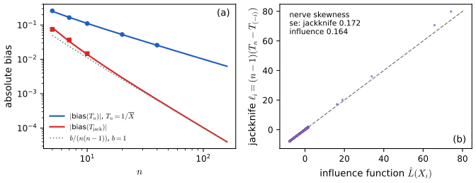
fig_3_s1. Download: PDF · SVG3.2 The Bootstrap
See also Probability and Statistical Inference, Section 8.2: bootstrap variance estimation, with the Monte Carlo and statistical errors measured.
pp. 30–31 The bootstrap (Efron 1979) estimates the variance and the distribution of \(T_n=g(X_1,\dots,X_n)\). Its variance \(\V_F(T_n)\) depends on \(F\); for the mean, \(\V_F(\Xbar)=\big(\int x^2\d F-(\int x\,\d F)^2\big)/n\). The bootstrap uses the plug-in estimate \(\V_{\Fn}(T_n)\), and since that is rarely computable in closed form, approximates it by simulation.
Algorithm 3.A (bootstrap variance estimation) p. 30, (3.11)
- Draw \(X_1^*,\dots,X_n^*\sim\Fn\), i.e. draw \(n\) points with replacement from the data.
- Compute \(T_n^*=g(X_1^*,\dots,X_n^*)\).
- Repeat steps 1 and 2 \(B\) times, giving \(T^*_{n,1},\dots,T^*_{n,B}\).
- Return
By the strong law of large numbers applied to the iid (given the data) replications, \(\vboot\to\V_{\Fn}(T_n)\) almost surely as \(B\to\infty\), and \(\seboot=\sqrt{\vboot}\). The book summarises the two approximations as \(\V_F(T_n)\approx\V_{\Fn}(T_n)\) with an error of order \(O(1/\sqrt n)\), and \(\V_{\Fn}(T_n)\approx\vboot\) with an error of order \(O(1/\sqrt B)\).
Filling the gap 3.6: the two error terms of the bootstrap p. 30
The orders refer to relative errors, for a smooth statistic: \(\V_{\Fn}(T_n)/\V_F(T_n)=1+\OP(n^{-1/2})\), and \(\vboot/\V_{\Fn}(T_n)=1+\OP(B^{-1/2})\).
Derivation
Statistical error. For the mean, \(\V_{\Fn}(\Xbar)=\hs^2/n\) exactly (each \(X_i^*\) has mean \(\Xbar\) and variance \(\hs^2\) under \(\Fn\)), and \(\V_F(\Xbar)=\sigma^2/n\). If \(\E X^4<\infty\), the central limit theorem gives \(\sqrt n(\hs^2-\sigma^2)\convd\N(0,\mu_4-\sigma^4)\), so the relative error is \(\hs^2/\sigma^2-1=\OP(n^{-1/2})\). For \(T_n=g(\Xbar)\) the leading terms are \(g'(\Xbar)^2\hs^2/n\) and \(g'(\mu)^2\sigma^2/n\), whose ratio is again \(1+\OP(n^{-1/2})\) because \(g'(\Xbar)-g'(\mu)=\OP(n^{-1/2})\). For the median the relative error is only \(\OP(n^{-1/4})\) (Hall and Martin 1988), so the \(O(n^{-1/2})\) of the diagram is the smooth case.
Monte Carlo error. Given the data, \(\vboot\) is the divisor-\(B\) variance of \(B\) iid draws from the bootstrap distribution, with kurtosis \(\kappa^*\). By the central limit theorem and the delta method, \(\sqrt B(\vboot/\V_{\Fn}(T_n)-1)\convd\N(0,\kappa^*-1)\), and the relative error of \(\seboot\) is about \(\sqrt{(\kappa^*-1)/(4B)}\): 2.2% at \(B=1000\) for a Normal-shaped bootstrap distribution. The full derivation is in the companion course (Filling the gap 8.2). Since \(B\) is ours to choose, the statistical error dominates.
Drawing from \(\Fn\) is drawing with replacement from the data, because \(\Fn\) gives probability \(1/n\) to each data point (with multiplicities if there are ties).
Algorithm 3.B (bootstrapping the median; the book's Figure 3.1) p. 31, Example 3.12
T     = median(X)                     # X = (X_1, ..., X_n)
Tboot = vector of length B
for b in 1, ..., B:
    Xstar    = n draws from X with replacement
    Tboot[b] = median(Xstar)
se = sqrt(variance(Tboot))
The book's pseudo-code loops to N where it means B. In the Python code, boot_reps(x, np.median, B, rng) followed by np.std is this algorithm.
The bootstrap also approximates the whole cdf \(G_n(t)=\P(T_n\le t)\) of the statistic:
\[ \widehat G^*_n(t)=\frac1B\sum_{b=1}^BI\big(T^*_{n,b}\le t\big). \tag{3.13} \]3.3 Parametric Bootstrap
See also Statistical Learning: Theory and Methods, Section 8.2: the parametric bootstrap agrees with maximum likelihood in Gaussian models.
p. 31 If \(F=F_\th\) belongs to a parametric family and \(\widehat\th\) estimates \(\th\), the parametric bootstrap draws the resamples from \(F_{\widehat\th}\) instead of \(\Fn\). It replaces the analytic work of the delta method by simulation, and when the model is right it is as accurate. When the model is wrong it estimates the variability of the wrong thing: in Exercise 3.5 a lognormal fit to the nerve data gives replications of the skewness centred near 5.4 for a sample skewness of 1.76. Where the nonparametric bootstrap fails (the maximum of uniform data, Exercise 3.11), a correct parametric model can rescue it.
Example 3.14 (the nerve data). p. 31 With \(B=1000\) nonparametric resamples, the bootstrap standard error of the skewness is 0.16 in the book; our run gives 0.165 (the ideal value, from \(10^5\) replications, is 0.163), close to the jackknife's 0.172. Despite its placement in Section 3.3, this example uses the ordinary, nonparametric bootstrap.
3.4 Bootstrap Confidence Intervals
See also Probability and Statistical Inference, Section 8.3: the Normal, pivotal and percentile intervals and their coverage.
pp. 32–34 Normal interval. \(T_n\pm z_{\alpha/2}\seboot\). It is accurate only if \(T_n\) is close to Normal.
Pivotal interval. Let \(\th=T(F)\), \(\hth=T(\Fn)\), and let \(H(r)=\P_F(R_n\le r)\) be the cdf of the pivot \(R_n=\hth-\th\). The interval \(C_n^\star=(a,b)\) with \(a=\hth-H^{-1}(1-\alpha/2)\) and \(b=\hth-H^{-1}(\alpha/2)\) has coverage exactly \(1-\alpha\). The bootstrap estimates \(H\) by \(\widehat H(r)=B^{-1}\sum_bI(R^*_{n,b}\le r)\) with \(R^*_{n,b}=\th^*_{n,b}-\hth\), and with \(\th^*_\beta\) the \(\beta\) sample quantile of the replications this yields
\[ C_n=\Big(2\hth-\th^*_{((1-\alpha/2)B)},\;2\hth-\th^*_{((\alpha/2)B)}\Big). \tag{3.15} \]Filling the gap 3.7: the exact pivotal interval, and the reflection in (3.15) pp. 32–33
Derivation
Exactness needs \(H\) continuous. \[ \P(a\le\th\le b)=\P(\hth-b\le R_n\le\hth-a)=\P(H^{-1}(\alpha/2)\le R_n\le H^{-1}(1-\alpha/2)) \]. If \(H\) is continuous and strictly increasing, \(H(H^{-1}(u))=u\) and \(\P(R_n=r)=0\), so this is \((1-\alpha/2)-\alpha/2=1-\alpha\). (The book's chain of equalities writes \(H(\hth-a)-H(\hth-b)\), with \(\hth\) treated as fixed; the correct reading is the one above, with \(H^{-1}(\cdot)\) fixed numbers.) If \(H\) has atoms, as for statistics of discrete data, the coverage is only \(\ge1-\alpha\) with the generalised inverse.
The reflection. The \(\beta\) sample quantile of \(R^*_{n,b}=\th^*_{n,b}-\hth\) is \(r^*_\beta=\th^*_\beta-\hth\), because subtracting a constant shifts all order statistics. So \(a=\hth-r^*_{1-\alpha/2}=2\hth-\th^*_{1-\alpha/2}\) and \(b=2\hth-\th^*_{\alpha/2}\): the percentile interval reflected about \(\hth\). The two coincide exactly when the replications are symmetric about \(\hth\). This interval is called "basic" by Davison and Hinkley (1997).
Theorem 3.16 (the pivotal interval is asymptotically exact) p. 33
If \(T\) is Hadamard differentiable and \(C_n\) is (3.15), then \(\P_F(T(F)\in C_n)\to1-\alpha\).
The proof, from Theorem 3.21, is Exercise 3.4; the interval is pointwise and asymptotic.
Studentized pivotal interval. Let \(Z_n=(T_n-\th)/\seboot\) and \(Z^*_{n,b}=(T^*_{n,b}-T_n)/\hse^*_b\), where \(\hse^*_b\) is a standard error of \(T^*_{n,b}\) computed from the \(b\)-th resample alone. With \(z^*_\beta\) the \(\beta\) quantile of the \(Z^*_{n,b}\), the interval is
\[ \Big(T_n-z^*_{1-\alpha/2}\,\seboot,\;T_n-z^*_{\alpha/2}\,\seboot\Big). \]Filling the gap 3.9: what the studentized interval needs, and the se inside each resample pp. 33–35
Derivation
The coverage calculation is the pivotal one with \(Z_n\) in place of \(R_n\): \(\P(\th\in C_n)=\P(z^*_{\alpha/2}\le Z_n\le z^*_{1-\alpha/2})\), which is close to \(1-\alpha\) if the bootstrap law of \(Z^*\) is close to the law of \(Z_n\). Two choices matter.
The scale of \(Z^*\) must be computed like the scale of \(Z_n\). In the real world the denominator is a function of the data; in the bootstrap world it must be the same function of the resample, \(\hse^*_b=\hse(X^*_{b,1},\dots,X^*_{b,n})\). Dividing \(T^*-T_n\) by the fixed \(\seboot\) would just rescale the pivotal interval. This is why one needs a standard error for each replication: by a second-level bootstrap (\(B\times B_2\) evaluations), or, as in Example 3.17, by a formula. For the skewness the formula is the nonparametric delta method on the resample, \(\hse^*_b=n^{-1}\big(\sum_iL_{\widehat F^*_b}(X^*_{b,i})^2\big)^{1/2}\), with the influence function of Exercise 3.1 evaluated at the resample's own mean, variance and skewness.
Which denominator for \(Z_n\). Theory (Section 3.5) prefers \(Z_n=(T_n-\th)/\hse\) with \(\hse\) the same formula applied to the data; the book uses \(\seboot\), which differs from it by \(\OP(n^{-1/2})\) relatively plus Monte Carlo error. For the nerve skewness the two are 0.165 and 0.164, and the intervals agree to two decimals. In the accuracy experiment of Figure 3.S4 the formula is used for both, so that the pivot is exactly studentized.
A caveat. If some resamples have a tiny \(\hse^*\), their \(Z^*\) is huge and the interval can become absurdly wide: for the law school correlation with \(n=15\), resamples with nearly collinear points do this (Exercise 3.2).
Percentile interval. \(C_n=\big(T^*_{(B\alpha/2)},T^*_{(B(1-\alpha/2))}\big)\), the \(\alpha/2\) and \(1-\alpha/2\) quantiles of the replications. The book justifies it by assuming a monotone transformation \(U=m(T)\) with \(U\sim\N(\phi,c^2)\), \(\phi=m(\th)\).
Filling the gap 3.8: the percentile interval, with the bootstrap quantiles centred correctly p. 34
Assume an increasing \(m\) with \(m(T_n)\sim\N(\phi,c^2)\) under \(F\), and that the same holds in the bootstrap world: \(m(T^*)\sim\N(m(T_n),c^2)\) under \(\Fn\). Then the percentile interval has coverage \(1-\alpha\) (exactly, for \(B=\infty\)).
Proof
Put \(U=m(T_n)\) and \(U^*=m(T^*)\). An increasing map preserves quantiles, so the \(\beta\) quantile of the \(U^*\) is \(m(T^*_{(B\beta)})\). In the bootstrap world the centre is \(U\), the transformed estimate, not the unknown \(\phi\): \(U^*_{(B\alpha/2)}=U-z_{\alpha/2}c\) and \(U^*_{(B(1-\alpha/2))}=U+z_{\alpha/2}c\). (The book writes \(\phi-z_{\alpha/2}c\approx U-z_{\alpha/2}c\); the first expression is not correct, the second is the right one and is exact under the assumption.) Therefore
\[ \P\big(T^*_{(B\alpha/2)}\le\th\le T^*_{(B(1-\alpha/2))}\big)=\P\big(U-z_{\alpha/2}c\le\phi\le U+z_{\alpha/2}c\big)=\P\Big(\Big|\frac{U-\phi}c\Big|\le z_{\alpha/2}\Big)=1-\alpha. \]We never need to know \(m\). What we do need is that the bootstrap reproduces the normalising transformation and the scale \(c\); when \(c\) depends on \(\phi\) or \(U\) has a bias, the argument fails, and the bias-corrected and accelerated (BC\(_a\)) interval of Efron (1987) adjusts for both. The companion course discusses the same correction (Filling the gap 8.9). ∎
Example 3.17 (the nerve-data skewness). pp. 34–35 The four 95% intervals, from the book and from our run (\(B=1000\), the resamples of the demonstration page with seed 1; studentized with the delta-method \(\hse^*\) of each resample):
| Method | book | our run |
|---|---|---|
| Normal | (1.44, 2.09) | (1.44, 2.08) |
| percentile | (1.42, 2.03) | (1.43, 2.06) |
| pivotal | (1.48, 2.11) | (1.46, 2.09) |
| studentized | (1.45, 2.28) | (1.47, 2.31) |
The first three agree with the book to within the Monte Carlo variation of \(B=1000\) (about 0.02 for an endpoint). The studentized interval is longer on the right, because the studentized replications have a long left tail (Figure 3.S2(b)): a resample with a large skewness also has a large \(\hse^*\), so \(Z^*\) is compressed on the right and stretched on the left, and the interval, which reflects the quantiles of \(Z^*\), reaches further to the right.
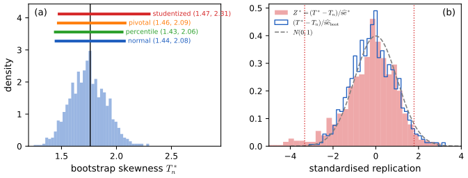
fig_3_s2. Download: PDF · SVG3.5 Some Theory
p. 35 Let \(\P_{\Fn}\) denote probability under resampling with the data held fixed, and let \(T_n=T(\Fn)\), \(T^*_n=T(\widehat F^*_n)\) with \(\widehat F^*_n\) the empirical cdf of a resample. Then, for \(u=\sqrt n(t-T(\Fn))\),
\[ \widehat G^*_n(t)=\P_{\Fn}\big(T(\widehat F^*_n)\le t\big)=\P_{\Fn}\big(\sqrt n(T(\widehat F^*_n)-T(\Fn))\le u\big), \tag{3.18} \](the book writes \(T(F)\) in the last expression, which with its \(u=\sqrt n(t-T(F))\) is the same event; the form above is the one compared with the sampling law in (3.20)). Consistency of the bootstrap means that the bootstrap law of \(\sqrt n(T^*_n-T_n)\) is close to the sampling law of \(\sqrt n(T_n-T(F))\), uniformly.
Theorem 3.19 (bootstrap consistency for smooth functions of the mean) p. 35, (3.20)
Suppose \(\E X_1^2<\infty\), \(T_n=g(\Xbar)\) with \(g\) continuously differentiable at \(\mu=\E X_1\) and \(g'(\mu)\ne0\). Then
\[ \sup_u\Big|\P_{\Fn}\big(\sqrt n(T(\widehat F^*_n)-T(\Fn))\le u\big)-\P_F\big(\sqrt n(T(\Fn)-T(F))\le u\big)\Big|\convas0. \tag{3.20} \]Filling the gap 3.10: from the mean (the appendix) to \(g(\Xbar)\) p. 35
Proof
The appendix proves the case \(g(x)=x\): \(\sup_x|\widehat H_n(x)-H_n(x)|\to0\) a.s., where \(H_n\) is the law of \(\sqrt n(\Xbar-\mu)\) and \(\widehat H_n\) the bootstrap law of \(\sqrt n(\overline X^*_n-\Xbar)\) (Filling the gap 3.14). Both converge to \(\N(0,\sigma^2)\): \(H_n\) by the central limit theorem, and then \(\widehat H_n\) a.s. by the appendix result and the triangle inequality.
Now apply the delta method in each world. Real world: \[ \sqrt n(g(\Xbar)-g(\mu))=g'(\mu)\sqrt n(\Xbar-\mu)+o_{\mathrm P}(1)\convd\N(0,g'(\mu)^2\sigma^2) \]. Bootstrap world, for almost every data sequence: \(\overline X^*_n-\Xbar=O_{\P_*}(n^{-1/2})\) because \(\widehat H_n\) converges, and \(\Xbar\to\mu\); since \(g'\) is continuous at \(\mu\), the mean value theorem gives \[ \sqrt n(g(\overline X^*_n)-g(\Xbar))=g'(\mu)\sqrt n(\overline X^*_n-\Xbar)+o_{\P_*}(1)\convd\N(0,g'(\mu)^2\sigma^2) \]. Two sequences of distributions converging weakly to the same continuous limit converge to it uniformly (Pólya's theorem: pointwise convergence of cdfs to a continuous cdf is uniform), so the supremum in (3.20) tends to 0, almost surely. The condition \(g'(\mu)\ne0\) makes the limit nondegenerate, hence continuous. ∎
Definition (Hadamard differentiability) p. 35, used in Theorem 3.21
A functional \(T\) is Hadamard differentiable at \(F\) with respect to \(d(F,G)=\sup_x|F(x)-G(x)|\) if there is a continuous linear map \(L_F\) such that for every \(t_k\downarrow0\) and every sequence \(D_k\) with \(d(D_k,D)\to0\) and \(F+t_kD_k\) a distribution,
\[ \frac{T(F+t_kD_k)-T(F)}{t_k}\to L_F(D). \]Writing \(L_F(D)=\int L_F(x)\,\d D(x)\), the function \(L_F(x)\) is the influence function (3.9).
Theorem 3.21 (bootstrap consistency for Hadamard differentiable functionals) p. 35, (3.22)
If \(T\) is Hadamard differentiable with respect to \(d\) and \(0<\int L_F^2(x)\,\d F(x)<\infty\), then
\[ \sup_u\Big|\P_{\Fn}\big(\sqrt n(T(\widehat F^*_n)-T(\Fn))\le u\big)-\P_F\big(\sqrt n(T(\Fn)-T(F))\le u\big)\Big|\convp0. \tag{3.22} \]Filling the gap 3.11: the functional delta method in both worlds p. 35
The proof combines three facts: Donsker's theorem for \(\sqrt n(\Fn-F)\), its bootstrap version for \(\sqrt n(\widehat F^*_n-\Fn)\), and the functional delta method. Here is the argument with the empirical-process facts quoted (van der Vaart 1998, Theorems 19.3, 20.8 and 23.7).
Proof
Real world. Donsker: \(\mathbb G_n=\sqrt n(\Fn-F)\convd\mathbb G\), a Brownian bridge composed with \(F\), in the space of bounded functions with the sup norm. Put \(t_n=n^{-1/2}\), \(D_n=\mathbb G_n\); then \(\Fn=F+t_nD_n\), and Hadamard differentiability with the continuous mapping theorem (in its "extended" form for converging sequences of maps) gives
\[ \sqrt n(T(\Fn)-T(F))=\frac{T(F+t_n\mathbb G_n)-T(F)}{t_n}\convd L_F(\mathbb G)=\N\Big(0,\int L_F^2\,\d F\Big). \]The variance: \(L_F(\mathbb G)\) is the limit of \(\sqrt n\,n^{-1}\sum_i L_F(X_i)\), which has mean 0 (\(\int L_F\,\d F=0\)) and variance \(\int L_F^2\,\d F\).
Bootstrap world. Conditionally on the data, \(\mathbb G^*_n=\sqrt n(\widehat F^*_n-\Fn)\convd\mathbb G\) in probability (Giné and Zinn 1990; this is where the convergence in (3.22) is only in probability, without extra conditions). Since \(\widehat F^*_n=\Fn+t_n\mathbb G^*_n\) and \(\Fn=F+t_n\mathbb G_n\), Hadamard differentiability at \(F\) applied twice, \[ T(\widehat F^*_n)-T(\Fn)=[T(F+t_n(\mathbb G_n+\mathbb G^*_n))-T(F)]-[T(F+t_n\mathbb G_n)-T(F)] \], gives \(\sqrt n(T(\widehat F^*_n)-T(\Fn))=L_F(\mathbb G^*_n)+o(1)\) in conditional probability, which converges to the same Normal law.
Uniformity. The common limit is continuous because \(\int L_F^2\,\d F>0\), so Pólya's theorem turns the two weak convergences into (3.22). ∎
Examples. Smooth functions of finitely many moments (mean, variance, skewness, correlation) are Hadamard differentiable when the moments involved exist; quantiles \(F^{-1}(p)\) are Hadamard differentiable at \(F\) with a positive density at the quantile, which is why the bootstrap, unlike the jackknife, works for the median. The maximum is not: its "derivative" is not continuous in \(d\), and the bootstrap fails (Exercise 3.11).
Results like these are why the bootstrap "works", and why it should not be applied blindly: they need regularity conditions. Under some conditions on \(T\) the bootstrap variance estimate is also consistent; the conditions are weaker than for the jackknife (the median is the standard example).
p. 36 Accuracy. A one-sided interval \([\th_\alpha,\infty)\) with nominal level \(1-\alpha\) is first-order accurate if \(\P(\th\le\th_\alpha)=\alpha+O(n^{-1/2})\), and second-order accurate if the error is \(O(n^{-1})\). The Normal, basic pivotal and percentile intervals are first-order accurate; the studentized pivotal and the adjusted percentile (BC\(_a\)) intervals are second-order accurate. The explanation is an Edgeworth expansion: with \(Z_n=\sqrt n(T_n-\th)/\sigma\),
\[ \P_F(Z_n\le z)=\Phi(z)+\frac1{\sqrt n}a(z)\phi(z)+O\Big(\frac1n\Big) \tag{3.23} \]for a polynomial \(a\) involving the skewness, and the bootstrap version satisfies
\[ \P_{\Fn}(Z^*_n\le z)=\Phi(z)+\frac1{\sqrt n}\hat a(z)\phi(z)+\OP\Big(\frac1n\Big),\qquad \hat a(z)-a(z)=\OP(n^{-1/2}). \tag{3.24} \]Filling the gap 3.12: the Edgeworth expansion of a standardised and of a studentized mean p. 36
Let \(X\) have mean \(\mu\), variance \(\sigma^2\), skewness \(\gamma=\E(X-\mu)^3/\sigma^3\), \(\E X^4<\infty\), and a nonlattice distribution (Cramér's condition \(\limsup_{|t|\to\infty}|\E e^{itX}|<1\)). Then
\[ \P\Big(\frac{\sqrt n(\Xbar-\mu)}\sigma\le z\Big)=\Phi(z)-\frac{\gamma(z^2-1)}{6\sqrt n}\phi(z)+o\Big(\frac1{\sqrt n}\Big),\qquad \P\Big(\frac{\sqrt n(\Xbar-\mu)}{\hs}\le z\Big)=\Phi(z)+\frac{\gamma(2z^2+1)}{6\sqrt n}\phi(z)+o\Big(\frac1{\sqrt n}\Big), \]uniformly in \(z\); with more moments the \(o(n^{-1/2})\) is \(O(n^{-1})\). So \(a(z)=-\gamma(z^2-1)/6\) for the standardised mean and \(a(z)=\gamma(2z^2+1)/6\) for the studentized one.
Derivation
Standardised mean. Let \(Y=(X-\mu)/\sigma\) and \(Z_n=n^{-1/2}\sum_iY_i\). The cumulants of \(Z_n\) are \(\kappa_1=0\), \(\kappa_2=1\), \(\kappa_3=\gamma/\sqrt n\), \(\kappa_4=O(1/n)\), because cumulants add over independent terms and scale as \(\kappa_r(cY)=c^r\kappa_r(Y)\). Its characteristic function is therefore
\[ \E e^{itZ_n}=\exp\Big(-\frac{t^2}2+\frac{\gamma(it)^3}{6\sqrt n}+O\Big(\frac{t^4}n\Big)\Big)=e^{-t^2/2}\Big(1+\frac{\gamma(it)^3}{6\sqrt n}\Big)+O\Big(\frac{(|t|^4+|t|^6)e^{-t^2/4}}n\Big)\quad\text{for }|t|\le\epsilon\sqrt n. \]Now \(e^{-t^2/2}\) is the Fourier transform of \(\phi\), and \((it)^3e^{-t^2/2}\) is that of \(-\phi'''\) (each derivative of the density multiplies the transform by \(-it\)). Inverting, the density expansion is \(\phi(z)-\frac\gamma{6\sqrt n}\phi'''(z)\), and integrating, \(\P(Z_n\le z)\approx\Phi(z)-\frac\gamma{6\sqrt n}\phi''(z)\). Since \(\phi''(z)=(z^2-1)\phi(z)\), this is the stated expansion. Making the inversion rigorous (Esseen's smoothing lemma, splitting the \(t\)-integral at \(\epsilon\sqrt n\) and using Cramér's condition for large \(|t|\)) is done in Hall (1992), Section 2.4.
Studentized mean. Write \(\hs^2=\sigma^2(1+\Delta)\) with \[ \Delta=n^{-1}\sum_i(Y_i^2-1)-\bar Y^2=W/\sqrt n+\OP(n^{-1}) \], where \(W=n^{-1/2}\sum_i(Y_i^2-1)\). Then the studentized statistic is \[ t_n=Z_n(1+\Delta)^{-1/2}=Z_n-Z_nW/(2\sqrt n)+\OP(n^{-1}) \]. The pair \((Z_n,W)\) is asymptotically jointly Normal with \(\E Z_n^2=1\) and \(\E(Z_nW)=\E[Y(Y^2-1)]=\gamma\). To order \(n^{-1/2}\):
- mean: \(\E t_n=-\E(Z_nW)/(2\sqrt n)=-\gamma/(2\sqrt n)\);
- variance: \(1+O(n^{-1})\);
- third moment: \[ \E t_n^3=\E Z_n^3-\tfrac3{2\sqrt n}\E(Z_n^3W)=\tfrac{\gamma}{\sqrt n}-\tfrac{9\gamma}{2\sqrt n}=-\tfrac{7\gamma}{2\sqrt n} \], using \(\E Z_n^3=\gamma/\sqrt n\) and the Gaussian moment identity \(\E(Z^3W)=3\E(Z^2)\E(ZW)\) to leading order;
- third cumulant: \[ \kappa_3=\E t_n^3-3\E t_n\,\E t_n^2+2(\E t_n)^3=-\tfrac{7\gamma}{2\sqrt n}+\tfrac{3\gamma}{2\sqrt n}=-\tfrac{2\gamma}{\sqrt n} \].
A statistic with mean \(m\), variance \(1+O(n^{-1})\) and third cumulant \(\kappa_3\), with \(m,\kappa_3\) of order \(n^{-1/2}\), has \[ \P(t_n\le z)=\Phi(z)-m\phi(z)-\frac{\kappa_3}6(z^2-1)\phi(z)+o(n^{-1/2}) \] by the same inversion. Here this is
\[ \Phi(z)+\frac{\gamma}{2\sqrt n}\phi(z)+\frac{2\gamma}{6\sqrt n}(z^2-1)\phi(z)=\Phi(z)+\frac{\gamma}{6\sqrt n}\big(3+2z^2-2\big)\phi(z), \]which is \(\Phi(z)+\gamma(2z^2+1)\phi(z)/(6\sqrt n)\). The sign is opposite to the standardised case: for right-skewed data, \(\hs\) is large exactly when \(\Xbar\) is large, which pulls the studentized statistic to the left. Both expansions are confirmed numerically for exponential data (Figure 3.S4(b) shows the first against the exact Gamma law).
Subtracting (3.24) from (3.23),
\[ \P_F(Z_n\le z)-\P_{\Fn}(Z^*_n\le z)=\OP\Big(\frac1n\Big). \tag{3.25} \]For the unstudentized \(V_n=\sqrt n(T_n-\th)\), on the other hand, \[ \P_F(V_n\le z)=\Phi(z/\sigma)+n^{-1/2}b(z/\sigma)\phi(z/\sigma)+O(n^{-1}) \] while the bootstrap gives the same with \(\hs\) for \(\sigma\), and since \(\hs=\sigma+\OP(n^{-1/2})\),
\[ \P_F(V_n\le z)-\P_{\Fn}(V^*_n\le z)=\OP\Big(\frac1{\sqrt n}\Big). \tag{3.26} \]Filling the gap 3.13: from (3.25) and (3.26) to the coverage of one-sided bounds pp. 36–37
Derivation
Why (3.26) is only \(n^{-1/2}\). The leading term of the difference is \(\Phi(z/\sigma)-\Phi(z/\hs)\approx\phi(z/\sigma)\frac z{\sigma^2}(\hs-\sigma)\), and \(\hs-\sigma\) is of exact order \(n^{-1/2}\) (it has a nondegenerate Normal limit after multiplying by \(\sqrt n\)). The bootstrap of an unstudentized statistic must estimate the scale, and pays a first-order price for it. A studentized statistic has scale 1 in both worlds; only the polynomial \(a\) has to be estimated, and it enters already multiplied by \(n^{-1/2}\).
Coverage of the studentized lower bound. Let \(\th_\alpha=T_n-\hse\,z^*_{1-\alpha}\), with \(z^*_{1-\alpha}\) the bootstrap quantile. Then \(\P(\th<\th_\alpha)=\P(Z_n>z^*_{1-\alpha})\). By (3.24), \(z^*_{1-\alpha}=z_\alpha-n^{-1/2}\hat a(z_\alpha)+\OP(n^{-1})\) (a Cornish–Fisher inversion), and by (3.23) the true quantile is the same expression with \(a\); they differ by \(\OP(n^{-1})\). A careful version of this argument (Hall 1992, Section 3.5, which handles the dependence between \(Z_n\) and \(z^*_{1-\alpha}\)) gives \(\P(\th<\th_\alpha)=\alpha+O(n^{-1})\).
Coverage of the others. The Normal bound uses \(z_\alpha\) in place of the true quantile \(z_\alpha-n^{-1/2}a(z_\alpha)\), an error of order \(n^{-1/2}\) that does not vanish unless \(a(z_\alpha)=0\) (no skewness). The basic pivotal bound uses the bootstrap law of \(V^*_n\), which by (3.26) is off by order \(n^{-1/2}\). The percentile bound uses the quantile of \(T^*\), i.e. of \(V^*\) reflected, and the sign of the skewness term is reversed, again an \(n^{-1/2}\) error. For two-sided equal-tailed intervals the \(n^{-1/2}\) terms cancel between the two tails (\(a\) is even), and all four have coverage error \(O(n^{-1})\); the difference is in where the misses fall, which matters for one-sided bounds and tests.
Numerical confirmation. For the mean of \(\Exp(1)\) data, Figure 3.S4(a) estimates \(\P(\mu<\th_{.05})\) with 20 000 data sets per \(n\). The errors of the Normal, pivotal and percentile bounds fall from about 0.023 to 0.011 as \(n\) goes from 10 to 160, a slope near \(-1/2\); the studentized error falls from 0.021 to below the Monte Carlo resolution (0.003) by \(n=40\).
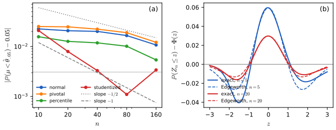
fig_3_s4. Download: PDF · SVG3.6 Bibliographic Remarks
p. 37 The jackknife is due to Quenouille (1949) and Tukey (1958), the bootstrap to Efron (1979). Book-length treatments: Efron and Tibshirani (1993), Davison and Hinkley (1997), Hall (1992) and Shao and Tu (1995); the empirical-process view is in Section 3.6 of van der Vaart and Wellner (1996).
3.7 Appendix
pp. 37–39 Two proofs that the bootstrap is consistent for the mean, following Section 3.1 of Shao and Tu (1995). Let \(H_n(t)=\P_F(\sqrt n(\Xbar-\mu)\le t)\) and \(\widehat H_n(t)=\P_{\Fn}(\sqrt n(\overline X^*_n-\Xbar)\le t)\). The goal is \(\sup_t|\widehat H_n(t)-H_n(t)|\to0\) almost surely.
Mallows' metric (Bickel and Freedman 1981). For random variables \(X\sim F\) and \(Y\sim G\), \(d_r(F,G)=\inf(\E|X-Y|^r)^{1/r}\), the infimum over all joint laws with marginals \(F\) and \(G\). The book lists its properties and the chain
\[ d_2(\widehat H_n,H_n)\le d_2(X_1^*-\Xbar,\,X_1-\mu)=\sqrt{d_2(\Fn,F)^2-(\mu-\Xbar)^2}\convas0. \]Filling the gap 3.14: the facts about Mallows' metric, proved, and the passage to the sup norm pp. 37–38
Proof
(i) Scaling. A coupling \((X,Y)\) gives the coupling \((aX,aY)\) of the scaled laws and conversely, with \(\E|aX-aY|^r=|a|^r\E|X-Y|^r\); take infima.
(ii) Centring identity. For any coupling, \[ \E(X-Y)^2=\E\big((X-\E X)-(Y-\E Y)\big)^2+(\E X-\E Y)^2 \], since the cross term has a mean-zero factor. The couplings of \((X,Y)\) and of the centred pair are the same, so taking infima gives \[ d_2(X,Y)^2=d_2(X-\E X,Y-\E Y)^2+(\E X-\E Y)^2 \].
(iii) Sums of independent mean-matched terms. Let \(X_1,\dots,X_m\) be independent, \(Y_1,\dots,Y_m\) independent, \(\E X_j=\E Y_j\). For each \(j\) take an optimal (or \(\epsilon\)-optimal) coupling \((X_j',Y_j')\), independently over \(j\). Then \((\sum X_j',\sum Y_j')\) couples the two sums, and the differences \(X_j'-Y_j'\) are independent with mean 0, so \(\E(\sum_j(X_j'-Y_j'))^2=\sum_j\E(X_j'-Y_j')^2\). Hence \(d_2(\sum X_j,\sum Y_j)^2\le\sum_jd_2(X_j,Y_j)^2\).
(iv) \(d_2(\Fn,F)\to0\) a.s. when \(\E X^2<\infty\). In one dimension the optimal coupling is the quantile coupling, \(d_2(F,G)^2=\int_0^1(F^{-1}(u)-G^{-1}(u))^2\d u\). By Glivenko–Cantelli, \(\Fn\to F\) uniformly a.s., hence \(\Fn^{-1}(u)\to F^{-1}(u)\) at every continuity point \(u\) of \(F^{-1}\), i.e. for almost every \(u\). By the strong law, \[ \int(\Fn^{-1})^2\d u=n^{-1}\sum_iX_i^2\to\E X^2=\int(F^{-1})^2\d u \]. Pointwise convergence plus convergence of the \(L^2\) norms implies \(L^2\) convergence (the Riesz–Scheffé argument applied to \(f_n^2\)), so \(d_2(\Fn,F)\to0\) a.s.
The chain. \(\sqrt n(\overline X^*_n-\Xbar)=n^{-1/2}\sum_i(X_i^*-\Xbar)\) and \(\sqrt n(\Xbar-\mu)=n^{-1/2}\sum_i(X_i-\mu)\) are scaled sums of independent mean-zero terms (given the data for the first). By (i) and (iii), \[ d_2(\widehat H_n,H_n)^2\le n^{-1}\sum_id_2(X_i^*-\Xbar,X_i-\mu)^2=d_2(X^*_1-\Xbar,X_1-\mu)^2 \]. By (ii), with \(\Es X_1^*=\Xbar\), this equals \(d_2(\Fn,F)^2-(\Xbar-\mu)^2\), which tends to 0 a.s. by (iv) and the strong law.
From \(d_2\) to the sup norm. \(d_2\)-convergence implies weak convergence (by Markov's inequality on a near-optimal coupling, \(\P(|X_n-Y_n|>\epsilon)\to0\)). \(H_n\to\N(0,\sigma^2)\) by the central limit theorem, so \(\widehat H_n\to\N(0,\sigma^2)\) weakly a.s., and Pólya's theorem (the limit is continuous) makes both convergences uniform. Hence \(\sup_t|\widehat H_n(t)-H_n(t)|\to0\) a.s. ∎
Rates. Figure 3.S6(a) shows that for exponential data \(d_2(\Fn,F)\) decreases more slowly than \(n^{-1/2}\), close to \(\sqrt{\log n/n}\): the quantile coupling is dominated by the largest observations. The bootstrap error in the sup norm (panel (b)) does decrease like \(n^{-1/2}\), as Singh's argument and the Edgeworth expansion predict.
The Berry–Esseen route (Singh 1981). The Berry–Esseen bound states that for iid data with \(\E|X_1|^3<\infty\) and \(Z_n=\sqrt n(\Xbar-\mu)/\sigma\),
\[ \sup_z|\P(Z_n\le z)-\Phi(z)|\le\frac{33}4\,\frac{\E|X_1-\mu|^3}{\sqrt n\,\sigma^3}. \tag{3.27} \]Applied in the bootstrap world, to \(Z^*_n=\sqrt n(\overline X^*_n-\Xbar)/\hs\) (the book's display omits the factor \(\sqrt n\)),
\[ \sup_z|\P_{\Fn}(Z^*_n\le z)-\Phi(z)|\le\frac{33}4\,\frac{\sum_{i=1}^n|X_i-\Xbar|^3}{n^{3/2}\hs^{\,3}}. \tag{3.28} \]With \(d(F,G)=\sup_x|F(x)-G(x)|\) and \(\Phi_a(x)=\Phi(x/a)\), the left side of (3.28) is \(d(\widehat H_n,\Phi_{\hs})\), and
\[ d(\widehat H_n,H_n)\le d(\widehat H_n,\Phi_{\hs})+d(\Phi_{\hs},\Phi_\sigma)+d(\Phi_\sigma,H_n). \tag{3.29} \]Filling the gap 3.15: the three terms of (3.29), and the Marcinkiewicz strong law p. 39
Proof
Third term. \(d(\Phi_\sigma,H_n)\to0\) by the central limit theorem and Pólya's theorem. Second term. \(\hs\to\sigma\) a.s., and \(a\mapsto\Phi_a\) is continuous in \(d\) for \(a>0\): \[ d(\Phi_a,\Phi_b)=\sup_x|\Phi(x/a)-\Phi(x/b)|\le\frac{|b-a|}{\min(a,b)}\sup_yy\phi(y) \], by the mean value theorem in the scale.
First term. It is at most the right side of (3.28). Since \(\hs\to\sigma>0\) a.s., it suffices that \(n^{-3/2}\sum_i|X_i-\Xbar|^3\to0\) a.s. Using \(|X_i-\Xbar|^3\le4(|X_i|^3+|\Xbar|^3)\) and \(\Xbar\to\mu\), it suffices that \(n^{-3/2}\sum_i|X_i|^3\to0\). Apply the lemma below to \(Y_i=|X_i|^3\) with \(\delta=2/3\): \(\E Y^\delta=\E X^2<\infty\), and \(n^{-1/\delta}\sum_iY_i=n^{-3/2}\sum_i|X_i|^3\).
Lemma (Marcinkiewicz). If \(Y_i\ge0\) are iid with \(\E Y_1^\delta<\infty\) for some \(0<\delta<1\), then \(n^{-1/\delta}\sum_{i=1}^nY_i\to0\) a.s.
Proof. \(\sum_n\P(Y_n^\delta>n)\le\E Y_1^\delta<\infty\), so by Borel–Cantelli \(Y_n\le n^{1/\delta}\) eventually; only finitely many terms are truncated, which does not affect the limit. Let \(W_i=Y_iI(Y_i\le i^{1/\delta})\). Then
\[ \sum_{i\ge1}\frac{\E W_i}{i^{1/\delta}}=\E\Big[Y_1\sum_{i\ge\max(1,Y_1^\delta)}i^{-1/\delta}\Big]\le C\,\E\Big[Y_1\max(1,Y_1^\delta)^{1-1/\delta}\Big]\le C\,\big(\E Y_1^\delta+1\big)<\infty, \]using \(\sum_{i\ge k}i^{-1/\delta}\le Ck^{1-1/\delta}\) for real \(k\ge1\) (as \(1/\delta>1\)); when \(Y_1\ge1\) the bracket is \(Y_1\cdot Y_1^{\delta-1}=Y_1^\delta\), and when \(Y_1<1\) it is at most 1. So \(\sum_iW_i/i^{1/\delta}\) converges a.s. (a series of nonnegative terms with finite mean), and Kronecker's lemma, with the increasing weights \(i^{1/\delta}\), gives \(n^{-1/\delta}\sum_{i\le n}W_i\to0\). ∎
All three terms vanish, so \(d(\widehat H_n,H_n)\to0\) a.s. With \(\E|X|^3<\infty\) the first term is \(O(n^{-1/2})\) a.s., the second \(O(\sqrt{\log\log n/n})\) by the law of the iterated logarithm, and the third \(O(n^{-1/2})\) by Berry–Esseen: Singh's route gives a rate as well as consistency. The constant \(33/4\) is very conservative; in Figure 3.S6(b) the bound (3.28) exceeds 1 up to \(n=320\), while the actual distance is 0.12 at \(n=10\) and 0.02 at \(n=640\).
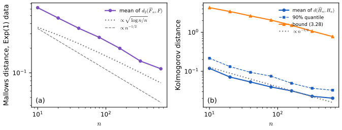
fig_3_s6. Download: PDF · SVGNotes on the book
The book's website has no errata list. Each item below gives the evidence.
Example 3.10 and Exercise 3.1: the influence function of the skewness lacks a term
The printed \[ L_F(x)=\frac{(x-\mu)^3}{\sigma^3}-T(F)\big(1+\frac32\frac{(x-\mu)^2-\sigma^2}{\sigma^2}\big) \] omits \(-3(x-\mu)/\sigma\), which comes from the dependence of the third central moment on the mean (Exercise 3.1). Both expressions have mean zero under \(F\), so that is no test; the derivative is. For \(F=\Exp(1)\) (\(\mu=\sigma=1\), \(T=2\)) and \(x=3\), the difference quotient \((T(F_\epsilon)-T(F))/\epsilon\) with \(\epsilon=10^{-6}\), computed from the exact moments of the mixture, is \(-8.99997\); the correct formula gives \(-9\) and the printed one \(-3\). On the nerve data the printed expression gives \(\hse=0.180\), the book's 0.18; the correct one gives 0.164.
Theorem 3.7: the limit law is for even \(n\)
\((\chi^2_2/2)^2\) is the limit along even sample sizes; along odd sizes it is \((\chi^2_4/4)^2\) (Filling the gap 3.4). Both have been confirmed by simulation (for the median of exponential data, the mean of \(\vjack/\sigma_n^2\) is close to 2 for even and 1.5 for odd \(n\)).
Page 34: the bootstrap quantiles are centred at \(U\), not \(\phi\)
In the justification of the percentile interval, \(U^*_{(B\alpha/2)}=\phi-z_{\alpha/2}c\) should read \(U-z_{\alpha/2}c\): in the bootstrap world \(U^*\sim\N(U,c^2)\). The conclusion is unchanged (Filling the gap 3.8).
Pages 35 and 38: two small slips
In (3.20) a closing parenthesis is missing after \(T(F)\). On page 38, \(Z^*_n=(\overline X^*_n-\Xbar)/\hs\) should be \(\sqrt n(\overline X^*_n-\Xbar)/\hs\), as (3.28) and the next display require.
Exercise 3.2: the last GPA should be 2.96
The last law school's GPA is printed as 3.96, which is above every other value and outside the range of Efron's data. With 3.96 the correlation is 0.546; with 2.96 it is 0.776, the value quoted for these data in the companion book (Wasserman 2004, Example 8.6) and by Efron and Tibshirani (1993).
Exercise 3.3: the formula for \(\vboot\) is missing a term, and \(\hat\alpha_3\) must be signed
The ideal bootstrap variance of \(\overline X^{*2}_n\) is \(\frac{4\Xbar^2\hat\alpha_2}n+\frac{4\Xbar\hat\alpha_3}{n^2}+\frac{\hat\alpha_4}{n^3}+\frac{(2n-3)\hat\alpha_2^2}{n^3}\), with \(\hat\alpha_3=n^{-1}\sum_i(X_i-\Xbar)^3\) (no absolute value). Exact enumeration of all \(4^4\) resamples of (1, 2.5, 4, 7.5) gives 92.414, which this formula reproduces exactly; the printed formula with absolute moments gives 100.44 (Exercise 3.3).
Example 3.14 is a nonparametric bootstrap
It sits in Section 3.3 (parametric bootstrap) but resamples the data; its standard error 0.16 is reproduced by the nonparametric bootstrap (0.165 with \(B=1000\); ideal 0.163).
3.8 Exercises
All thirteen exercises of Chapter 3 (pp. 39–41), restated in my own words, with complete solutions (hidden). Computational answers come from ch03_bootstrap_jackknife.py.
Exercise 3.1. Find the influence function of the skewness \(T(F)=\int(x-\mu)^3\,\d F(x)/\sigma^3\).
Solution
Let \(F_\epsilon=(1-\epsilon)F+\epsilon\delta_x\) and differentiate at \(\epsilon=0\). The mean \(\mu_\epsilon=\mu+\epsilon(x-\mu)\) has derivative \(x-\mu\). For a central moment \(\mu_k(F_\epsilon)=\int(y-\mu_\epsilon)^k\d F_\epsilon(y)\), the product rule gives two terms: moving the measure contributes \((x-\mu)^k-\mu_k\), moving the centre contributes \(-k\mu_{k-1}(x-\mu)\). So
\[ L_{\sigma^2}(x)=(x-\mu)^2-\sigma^2\quad(\mu_1=0),\qquad L_{\mu_3}(x)=(x-\mu)^3-\mu_3-3\sigma^2(x-\mu). \]With \(T=\mu_3(\sigma^2)^{-3/2}\) the chain rule gives \(L_T=\sigma^{-3}L_{\mu_3}-\frac32\mu_3\sigma^{-5}L_{\sigma^2}\):
\[ L_F(x)=\frac{(x-\mu)^3}{\sigma^3}-\frac{3(x-\mu)}\sigma-T(F)\Big(1+\frac32\,\frac{(x-\mu)^2-\sigma^2}{\sigma^2}\Big). \]It has mean 0 under \(F\), as every influence function must, and the term \(-3(x-\mu)/\sigma\) is the one missing in the book's display. A numerical derivative confirms it (notes on the book), and the nerve-data standard error is \(\hse=0.164\). The companion course derives the same formula (Filling the gap 8.5).
Exercise 3.2. For Efron's law school data (15 schools, average LSAT and GPA), find the plug-in correlation; estimate its standard error by (i) the influence function, (ii) the jackknife and (iii) the bootstrap; then compute a 95% studentized pivotal interval, which needs a standard error of \(T^*\) for every resample.
Solution
With the last GPA read as 2.96 (notes on the book), \(r=0.776\). (i) The influence function of the correlation, with \(u,v\) the standardised coordinates, is \(L(x,y)=uv-\frac r2(u^2+v^2)\); then \(\hse=\sqrt{\sum_iL_i^2}/n=0.124\). (ii) \(\sejack=0.143\). (iii) With \(B=2000\), \(\seboot=0.133\). The intervals: Normal (0.52, 1.04), percentile (0.46, 0.97), pivotal (0.59, 1.09).
The studentized interval, with \(\hse^*_b\) the influence-function standard error of each resample, is (\(-0.69\), 1.01). Its lower end is absurd. The reason is visible in the demonstration: with 15 points, some resamples consist of few distinct schools that lie nearly on a line; their \(r^*\) is near 1 and their \(\hse^*\) near 0, so \(Z^*=(r^*-r)/\hse^*\) is enormous, the upper quantile \(z^*_{.975}\) explodes, and \(T_n-z^*_{.975}\seboot\) runs far to the left. Second-order accuracy is a large-sample property; at \(n=15\) for a bounded, skewed statistic, the variance-stabilised scale (Fisher's \(z=\operatorname{artanh}r\)) is the better place to studentize, giving \[ \tanh(\operatorname{artanh}r\pm1.96/\sqrt{12})=(0.44,0.92) \].
Exercise 3.3. For \(T_n=\Xbar^{\,2}\), with sample central moments \(\hat\alpha_k=n^{-1}\sum_i(X_i-\Xbar)^k\), compute the ideal bootstrap variance \(\vboot=\Vs(\overline X^{*2}_n)\).
Solution
Let \(D=\overline X^*_n-\Xbar\), a mean of \(n\) iid draws of \(X^*-\Xbar\), which has moments \(0,\hat\alpha_2,\hat\alpha_3,\hat\alpha_4\) under \(\Fn\). As in Filling the gap 3.1, \(\Es D^2=\hat\alpha_2/n\), \(\Es D^3=\hat\alpha_3/n^2\), \(\Es D^4=\hat\alpha_4/n^3+3(n-1)\hat\alpha_2^2/n^3\). Since \(\overline X^{*2}_n=\Xbar^2+2\Xbar D+D^2\),
\[ \Vs(\overline X^{*2}_n)=4\Xbar^2\Vs(D)+4\Xbar\Cov_*(D,D^2)+\Vs(D^2)=\frac{4\Xbar^2\hat\alpha_2}n+\frac{4\Xbar\hat\alpha_3}{n^2}+\frac{\hat\alpha_4}{n^3}+\frac{(2n-3)\hat\alpha_2^2}{n^3}, \]using \(\Cov_*(D,D^2)=\Es D^3\) and \(\Vs(D^2)=\Es D^4-(\Es D^2)^2\) with \(\frac{3(n-1)}{n^3}-\frac1{n^2}=\frac{2n-3}{n^3}\). The book's answer has no last term and uses absolute moments; the last term is of order \(n^{-2}\), the same order as the second. Exact enumeration of the \(4^4=256\) equally likely resamples of (1, 2.5, 4, 7.5) gives 92.414, equal to the formula above; the book's formula gives 100.44. For the nerve data the two differ in the fifth significant figure, because there \(n=799\).
Exercise 3.4. Prove Theorem 3.16.
Solution
Let \(\tau^2=\int L_F^2\,\d F\in(0,\infty)\), and let \(K_n\) and \(\widehat K_n\) be the cdfs of \(\sqrt n(\hth-\th)\) and of \(\sqrt n(\th^*_n-\hth)\) under resampling. By Filling the gap 3.11, \(K_n\to\Phi_\tau\) uniformly and, by Theorem 3.21, \(\sup_u|\widehat K_n(u)-K_n(u)|\convp0\); hence \(\sup_u|\widehat K_n(u)-\Phi_\tau(u)|\convp0\).
Quantiles converge. Fix \(\beta\in(0,1)\) and \(\epsilon>0\). Since \(\Phi_\tau\) is continuous and strictly increasing, \[ \eta=\min\{\beta-\Phi_\tau(\tau z_{1-\beta}-\epsilon),\Phi_\tau(\tau z_{1-\beta}+\epsilon)-\beta\}>0 \], where \(\tau z_{1-\beta}=\Phi_\tau^{-1}(\beta)\). On the event \(\sup|\widehat K_n-\Phi_\tau|<\eta\), whose probability tends to 1, the \(\beta\) quantile \(\hat k_\beta\) of \(\widehat K_n\) lies within \(\epsilon\) of \(\Phi_\tau^{-1}(\beta)\). So \(\hat k_\beta\convp\Phi_\tau^{-1}(\beta)\). (With finite \(B\), the empirical quantile of \(B\) replications adds an error that vanishes as \(B\to\infty\); the theorem is about the ideal bootstrap.)
Coverage. The pivotal interval is \(\hth-\hat k_{1-\alpha/2}/\sqrt n\le\th\le\hth-\hat k_{\alpha/2}/\sqrt n\), i.e. \(\hat k_{\alpha/2}\le\sqrt n(\hth-\th)\le\hat k_{1-\alpha/2}\). Since \(\sqrt n(\hth-\th)\convd\N(0,\tau^2)\) and the random endpoints converge in probability to constants, Slutsky's theorem gives
\[ \P_F(\th\in C_n)\to\Phi_\tau(\Phi_\tau^{-1}(1-\alpha/2))-\Phi_\tau(\Phi_\tau^{-1}(\alpha/2))=1-\alpha, \]where the limit at the endpoints is legitimate because \(\Phi_\tau\) is continuous. ∎
Exercise 3.5. Redo Example 3.17 with a parametric bootstrap that assumes the nerve data are lognormal: fit \(Y=\log X\sim\N(\mu,\sigma^2)\), draw \(Y^*_i\) from the fit and set \(X^*_i=e^{Y^*_i}\).
Solution
The fit is \(\hat\mu=-2.004\), \(\hat\sigma=1.080\) (divisor \(n\)). A lognormal law with \(\sigma=1.080\) has skewness \((e^{\sigma^2}+2)\sqrt{e^{\sigma^2}-1}=7.74\), far from the sample skewness 1.76. With \(B=2000\) parametric resamples, the replications of the skewness have mean 5.42 and standard deviation 2.51. The resulting 95% intervals around \(T_n=1.76\) are meaningless: Normal (\(-3.16\), 6.68), percentile (3.03, 12.38), pivotal (\(-8.85\), 0.49), studentized (\(-19.3\), \(-4.6\)). The percentile interval does not even contain the estimate.
The lesson: a parametric bootstrap estimates the sampling distribution under the fitted model, and is only as good as the model. The nerve times are much closer to exponential (skewness 2, a Gamma shape) than to lognormal; a log transform of such data is far from Normal (it is left-skewed), and the lognormal fit inflates the upper tail. The nonparametric bootstrap needs no such assumption.
Exercise 3.6 (computer experiment). With \(n=50\), \(Y_i\sim\N(0,1)\) and \(X_i=e^{Y_i}\), and \(T(F)\) the skewness of \(X\), build the four bootstrap 95% intervals, repeat many times, and estimate the true coverage of each.
Solution
The true skewness is \(\th=(e+2)\sqrt{e-1}=6.18\). With 500 data sets and \(B=500\) (Figure 3.S3), the coverages at \(n=50\) are Normal 0.11, pivotal 0.14, percentile 0.01, studentized 0.36. All are far below 0.95, and almost every miss is on the same side: the interval lies below \(\th\). Studentizing helps the most, but not enough.
The reason is structural. The skewness of a lognormal is driven by rare, very large values that a sample of 50 rarely contains, and the sample skewness is bounded: by the Cauchy–Schwarz inequality, \(|T(\Fn)|\le(n-2)/\sqrt{n-1}=6.86\) for \(n=50\). The plug-in estimate is therefore biased far downwards, its bootstrap distribution inherits the same limitation, and no interval built from it can reach 6.18 often. Increasing \(n\) helps slowly: at \(n=200\) the coverages are 0.22, 0.23, 0.15 and 0.48.
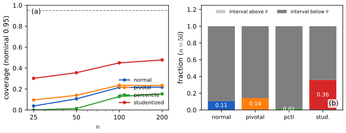
Figure 3.S3 (supplementary). Exercise 3.6: coverage of the four bootstrap intervals for the skewness of lognormal data, 500 data sets and \(B=500\) per \(n\); the studentized interval uses the influence-function standard error of each resample. (b) At \(n=50\), the fractions of intervals that cover \(\th\), lie above it, and lie below it. Not a figure of the book. Code: ch03_bootstrap_jackknife.py, fig_3_s3. Download: PDF · SVGExercise 3.7 (computer experiment). With \(n=25\), \(X_i\sim t_3\) and \(\th=(q_{.75}-q_{.25})/1.34\), compare by simulation the coverage and length of (i) the Normal interval with jackknife standard error, (ii) the Normal interval with bootstrap standard error, (iii) the percentile interval.
Solution
Here \(\th=2t_{3,.75}/1.34=1.142\). With 1000 data sets and \(B=500\) (sample quantiles by linear interpolation), the coverages are (i) 0.850, (ii) 0.946, (iii) 0.970, with mean lengths 1.22, 1.35 and 1.31. The jackknife interval undercovers, as Theorem 3.7 predicts: \(\vjack\) for a quantile does not converge to the true variance, and its ratio to the true variance keeps a nondegenerate spread as \(n\) grows, so it is often much too small, which costs coverage. The bootstrap standard error is consistent, and both bootstrap intervals are close to nominal.
Exercise 3.8. If \(X_1,\dots,X_n\) are distinct, show that there are \(\binom{2n-1}n\) distinct bootstrap samples.
Solution
A bootstrap sample, as an unordered multiset (which is all a symmetric statistic sees), is determined by the counts \((m_1,\dots,m_n)\) of how often each \(X_i\) is drawn, with \(m_i\ge0\) and \(\sum_im_i=n\); distinct data make distinct count vectors give distinct samples. Represent a count vector by a row of \(n\) balls and \(n-1\) bars separating the \(n\) buckets: every arrangement of \(2n-1\) symbols with \(n\) balls is one count vector and conversely. So there are \(\binom{2n-1}n\) of them. For \(n=4\): \(\binom74=35\); for \(n=10\): 92 378, against \(10^{10}\) ordered resamples.
Exercise 3.9. For distinct observations and a bootstrap sample with mean \(\overline X^*_n\), find \(\E(\overline X^*_n\given X_1,\dots,X_n)\), \(\V(\overline X^*_n\given X_1,\dots,X_n)\), \(\E(\overline X^*_n)\) and \(\V(\overline X^*_n)\).
Solution
Given the data, the \(X^*_i\) are iid from \(\Fn\), with mean \(\Xbar\) and variance \(\hs^2\). So \(\E(\overline X^*_n\given X)=\Xbar\) and \(\V(\overline X^*_n\given X)=\hs^2/n\). Unconditionally, \(\E\overline X^*_n=\E\Xbar=\mu\), and by the law of total variance, with \(\E\hs^2=(n-1)\sigma^2/n\),
\[ \V(\overline X^*_n)=\E\Big(\frac{\hs^2}n\Big)+\V(\Xbar)=\frac{(n-1)\sigma^2}{n^2}+\frac{\sigma^2}n=\frac{(2n-1)\sigma^2}{n^2}, \]almost twice \(\V(\Xbar)=\sigma^2/n\).
Exercise 3.10 (computer experiment). With \(X_i\sim\N(\mu,1)\), \(\th=e^\mu\) and the MLE \(\hth=e^{\Xbar}\), simulate \(n=100\) observations with \(\mu=5\). (a) Find the standard error and a 95% interval by the delta method, the parametric bootstrap and the nonparametric bootstrap. (b) Plot histograms of the parametric and nonparametric replications, compare them with the delta-method Normal approximation and with the true sampling distribution of \(\hth\), and say which is closest.
Solution
(a) In our sample \(\Xbar=4.806\), so \(\hth=122.2\) (the true \(\th=e^5=148.4\); this sample's mean happens to be 1.9 standard errors low). Delta method: \(\hse=e^{\Xbar}/\sqrt n=12.22\), interval (98.3, 146.2). Parametric bootstrap (\(B=4000\), \(X^*\sim\N(\Xbar,1)\)): \(\seboot=11.93\), percentile interval (100.3, 147.8). Nonparametric bootstrap: \(\seboot=10.46\), percentile interval (103.8, 144.6). All three intervals just miss \(\th\), as an interval of a 1.9-standard-error-low sample would.
(b) The true law of \(\hth\) is lognormal, \(\log\hth\sim\N(5,1/100)\), with a slight right skew. The parametric replications follow the same shape around \(\hth\) (they are exactly lognormal with parameters \((\Xbar,1/100)\)); the nonparametric ones are narrower here because the plug-in variance of this data set is 0.69 rather than 1; the delta method misses the skew. In shape, the parametric bootstrap is closest, because the model is correct. All three are centred at \(\hth\), not \(\th\) (Figure 3.S5(a)): a bootstrap estimates the spread and shape of the sampling distribution, never its location.
Exercise 3.11. Let \(X_i\sim\Unif(0,\th)\), with MLE \(\hth=X_{\max}\); generate 50 observations with \(\th=1\). (a) Find the distribution of \(\hth\) and compare it with histograms of parametric and nonparametric bootstrap replications. (b) Show that \(\P(\hth^*=\hth)=0\) for the parametric bootstrap but \(\approx0.632\) for the nonparametric one.
Solution
(a) \(\P(\hth\le t)=\P(\text{all }X_i\le t)=(t/\th)^n\), density \(nt^{n-1}/\th^n\) on \([0,\th]\). Parametric replications (maxima of 50 draws from \(\Unif(0,\hth)\)) have the same shape scaled by \(\hth\); the nonparametric replications are concentrated on the few largest data values, with a spike of about 63% at \(\hth\) itself (Figure 3.S5(b)).
(b) Under the parametric bootstrap \(\hth^*\) has a continuous law, so \(\P(\hth^*=\hth)=0\). Under the nonparametric one, \(\hth^*=\hth\) exactly when the resample contains the largest observation, so \[ \P_*(\hth^*=\hth)=1-(1-1/n)^n\to1-e^{-1}=0.632 \]; for \(n=50\) it is 0.636, and our 4000 replications give 0.634. The true law has no atom: \(n(\th-\hth)\) converges to an exponential law with mean \(\th\), so the bootstrap distribution of \(n(\hth-\hth^*)\) cannot converge to it: the nonparametric bootstrap is inconsistent for the maximum (the functional is not Hadamard differentiable). The companion course works this out in detail (Filling the gap 8.12).
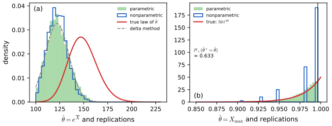
Figure 3.S5 (supplementary). Parametric against nonparametric bootstrap, 4000 replications each. (a) Exercise 3.10: \(\hth=e^{\Xbar}\) for 100 \(\N(5,1)\) observations; the true sampling density of \(\hth\) is centred at \(\th\), the bootstrap histograms and the delta-method curve at \(\hth\). (b) Exercise 3.11: the maximum of 50 \(\Unif(0,1)\) observations. Not a figure of the book. Code: ch03_bootstrap_jackknife.py, fig_3_s5. Download: PDF · SVGExercise 3.12. Fifty patients receive a placebo and fifty a new treatment; 30 placebo and 40 treated patients improve. Let \(\tau=p_2-p_1\). (a) Find the MLE of \(\tau\), its standard error and a 90% interval by the delta method. (b) Do the same with the bootstrap.
Solution
(a) \(\hat p_1=0.6\), \(\hat p_2=0.8\), \(\hat\tau=0.2\). The two groups are independent, so
\[ \hse=\sqrt{\frac{\hat p_1(1-\hat p_1)}{50}+\frac{\hat p_2(1-\hat p_2)}{50}}=\sqrt{0.0048+0.0032}=0.0894, \]and the 90% interval is \(0.2\pm1.645(0.0894)=(0.053,0.347)\).
(b) Resampling each group separately (keeping the design: 50 and 50), \(B=4000\) gives \(\seboot=0.0913\), Normal interval (0.050, 0.350) and percentile interval (0.04, 0.34). The bootstrap reproduces the delta method up to Monte Carlo error; the exact ideal value is \(\sqrt{0.6\cdot0.4/50+0.8\cdot0.2/50}=0.0894\) as well, since for a binomial proportion \(\V_{\Fn}\) is the plug-in variance. All intervals exclude 0.
Exercise 3.13. Each bootstrap draw \(X^*_i\) has the same marginal distribution \(F\) as \(X_i\) (since \(\P(X^*_i\le x)=\E\Fn(x)=F(x)\)), yet Exercise 3.9 showed \(\V(\overline X^*_n)\ne\V(\Xbar)\). Explain.
Solution
The marginals agree, but the joint law does not: \(X^*_1,\dots,X^*_n\) are independent only conditionally on the data. Unconditionally they are exchangeable but positively correlated, because they are all drawn from the same data set. For \(i\ne j\),
\[ \Cov(X^*_i,X^*_j)=\E\Cov(X^*_i,X^*_j\given X)+\Cov\big(\E(X^*_i\given X),\E(X^*_j\given X)\big)=0+\V(\Xbar)=\frac{\sigma^2}n. \]Hence \[ \V(\overline X^*_n)=\frac1{n^2}\big(n\sigma^2+n(n-1)\frac{\sigma^2}n\big)=\frac{(2n-1)\sigma^2}{n^2} \], matching Exercise 3.9. The variance of a mean depends on the joint law, not only on the marginals. This is also why the bootstrap is used conditionally: \(\V(\overline X^*_n\given X)=\hs^2/n\) estimates \(\V(\Xbar)\), while the unconditional \(\V(\overline X^*_n)\) mixes in the sampling variability of the data.
Demonstrations for this chapter
Each demonstration runs in the browser and links back to these notes.
| Demonstration | What you can see | Sections and results |
|---|---|---|
| The jackknife bias correction | Bias of \(T_n\) and \(\Tjack\) against \(n\), simulated and exact, for four statistics; leave-one-out values and pseudo-values of one data set. Presets: 1 \(1/\overline X\); 2 plug-in variance; 3 \(\exp(\overline X)\); 4 correlation, small \(n\); 5 one data set, \(n=80\). | Section 3.1; Filling the gaps 3.1, 3.2, 3.5 |
| Four bootstrap intervals | Replications, the Normal, percentile, pivotal and studentized intervals, and the studentized pivot, on the nerve data and the law school data. Presets: 1 Example 3.17; 2 Exercise 3.2; 3 the mean; 4 small \(B\); 5 99%. | Section 3.4; Filling the gaps 3.7, 3.8, 3.9; Exercise 3.2 |
| First- and second-order accuracy | Miss rates of the four one-sided bounds for a mean against \(n\), and the Edgeworth corrections. Presets: 1 exponential; 2 \(\chi^2_1\); 3 lognormal; 4 uniform; 5 Edgeworth at \(n=5\). | Section 3.5; Filling the gaps 3.12, 3.13 |
Related demonstrations in the companion course Probability and Statistical Inference: coverage of the three bootstrap intervals, the jackknife against the bootstrap and how many replications. The Python code for every figure on this page is code/ch03_bootstrap_jackknife.py; see the code index.
References
- Wasserman, L. (2006). All of Nonparametric Statistics. Springer, New York. Chapter 3, pp. 27–41. www.stat.cmu.edu/~larry/all-of-nonpar.
- Wasserman, L. (2004). All of Statistics: A Concise Course in Statistical Inference. Springer, New York. Chapter 8.
- Bickel, P. J. and Freedman, D. A. (1981). Some asymptotic theory for the bootstrap. The Annals of Statistics, 9(6), 1196–1217.
- Cox, D. R. and Lewis, P. A. W. (1966). The Statistical Analysis of Series of Events. Methuen, London.
- Davison, A. C. and Hinkley, D. V. (1997). Bootstrap Methods and Their Application. Cambridge University Press.
- Efron, B. (1979). Bootstrap methods: another look at the jackknife. The Annals of Statistics, 7(1), 1–26.
- Efron, B. (1982). The Jackknife, the Bootstrap and Other Resampling Plans. SIAM, Philadelphia.
- Efron, B. (1987). Better bootstrap confidence intervals. Journal of the American Statistical Association, 82(397), 171–185.
- Efron, B. and Tibshirani, R. J. (1993). An Introduction to the Bootstrap. Chapman and Hall, New York.
- Ghosh, M., Parr, W. C., Singh, K. and Babu, G. J. (1984). A note on bootstrapping the sample median. The Annals of Statistics, 12(3), 1130–1135.
- Giné, E. and Zinn, J. (1990). Bootstrapping general empirical measures. The Annals of Probability, 18(2), 851–869.
- Hall, P. (1992). The Bootstrap and Edgeworth Expansion. Springer, New York.
- Hall, P. and Martin, M. A. (1988). Exact convergence rate of bootstrap quantile variance estimator. Probability Theory and Related Fields, 80(2), 261–268.
- Quenouille, M. H. (1949). Approximate tests of correlation in time-series. Journal of the Royal Statistical Society, Series B, 11(1), 68–84.
- Shao, J. and Tu, D. (1995). The Jackknife and Bootstrap. Springer, New York.
- Singh, K. (1981). On the asymptotic accuracy of Efron's bootstrap. The Annals of Statistics, 9(6), 1187–1195.
- Tukey, J. W. (1958). Bias and confidence in not-quite large samples (abstract). The Annals of Mathematical Statistics, 29(2), 614.
- van der Vaart, A. W. (1998). Asymptotic Statistics. Cambridge University Press.
- van der Vaart, A. W. and Wellner, J. A. (1996). Weak Convergence and Empirical Processes. Springer, New York.
The numerical statements in the text (the nerve-data and law-school estimates and intervals, the exact jackknife biases, the influence-function standard errors, the corrected formula of Exercise 3.3, the coverage studies of Exercises 3.6 and 3.7, the Edgeworth expansions and the jackknife limit laws for the median) were confirmed numerically.