Nonparametric Inference Using Orthogonal Functions
Expand the unknown function in an orthonormal basis and the data turn into noisy coefficients: regression on an equally spaced design becomes, almost exactly, the many normal means problem of Chapter 7. That reduction does all the work in this chapter. A modulator shrinks the coefficients, Stein's unbiased risk estimate chooses the amount of shrinkage (the react method of Beran), the noise level is read off the highest coefficients, a pivot gives a confidence ball and the tube formula a band. Irregular designs are handled by orthonormalising the basis at the data points, densities by taking sample means of the basis functions, and several covariates by tensor products. The estimators are linear smoothers, so everything of Chapter 5 applies, and they are kernel smoothers in disguise, with a kernel that reflects at the end points.
Ch. 1 Introduction Ch. 2 The cdf and functionals Ch. 3 Bootstrap and jackknife Ch. 4 Smoothing Ch. 5 Regression Ch. 6 Density estimation Ch. 7 Normal means and minimax Ch. 8 Orthogonal functions Ch. 9 Wavelets Ch. 10 Other topics
How to read these notes
They follow the book. Sections carry the book's numbers (8.1 to 8.8), results keep the book's numbers (Lemma 8.4, Theorem 8.13, ...), and every displayed equation of the book keeps its number, e.g. \((8.18)\). Equations without a number are steps the book skips.
Filling the gaps. The chapter is short and states most of its results without proof: Lemma 8.4, Theorem 8.13 and equations (8.19) and (8.26) are left as exercises, the consistency of the noise estimate is asserted, and Theorems 8.17 and 8.23 are quoted from Beran and Dümbgen (1998). For each an orange Filling the gap box gives a complete argument with its assumptions. Two of them correct the book: the noise estimate (8.12) as printed is not consistent, and the variance in the confidence ball of Theorem 8.23 misses the contribution of the estimated noise level (Notes on the book). Proofs start hidden: open one with its bar, or use the button below.
Figures and demonstrations. Figures 8.1 and 8.2, the only figures of the chapter, are reproduced from scratch by the Python code. Supplementary figures (8.S1, 8.S2, ...) illustrate the gaps and the exercises. The ▶ Demo boxes open an interactive demonstration set to the case being discussed.
Main reference
L. Wasserman, All of Nonparametric Statistics, Springer (2006), Chapter 8, pages 183–195 (book website, with the data: www.stat.cmu.edu/~larry/all-of-nonpar). Section, equation, figure and exercise numbers below refer to this book. Further reading is listed in the references.
The explanations, derivations, figures and code are my own; equations are cited by their numbers in the book.
Companion courses
This chapter is the advanced sequel of Chapter 21 of Probability and Statistical Inference (the same author's All of Statistics), which develops the same estimators with a fixed number of terms:
- Section 8.2 (the cosine basis, the coefficients, the noise estimate, the risk estimate, the band): Probability and Statistical Inference, Section 21.1 (completeness of the cosine basis, Filling the gap 21.2; smoothness and decay, 21.4) and Section 21.3 (exact variances on the grid, Filling the gap 21.9; the noise level, 21.10), with its cosine regression band demo.
- Section 8.4 (density estimation, surgery): Probability and Statistical Inference, Section 21.2 (Filling the gaps 21.5 to 21.7) and its cosine density demo.
- The James–Stein estimator behind the constant modulator: Probability and Statistical Inference, Section 12.7 (Stein's paradox); SURE as Mallows' \(C_p\): Statistical Learning: Theory and Methods, Section 7.5.
- Section 8.6 (tensor products): Statistical Learning, Section 5.7 (multidimensional splines); kernel density estimates (Exercise 11): Bayesian and Probabilistic Machine Learning, Section 2.5.
Within this course, the chapter builds on Chapter 5 (linear smoothers, bands by the tube formula) and on Chapter 7 (normal means, Sobolev ellipsoids, SURE, Pinsker's theorem, confidence balls). Where a companion proof is complete, these notes state the result, sketch the argument and link to it. The effort here goes to what this chapter adds: data-driven choice of the modulator and why it works uniformly, the monotone modulator and the PAV algorithm, the noise estimate and its consistency, the confidence ball, irregular designs and tensor products.
The chapter at a glance
- 8.2 On the design \(x_i=i/n\) the cosine coefficients \(Z_j=n^{-1}\sum_iY_i\phi_j(x_i)\) are nearly independent \(\N(\th_j,\sigma^2/n)\); truncating at \(n\) terms costs \(O(n^{-2m})\) over a Sobolev ellipsoid (Lemma 8.4). A modulator \(b\) gives \(\hth=bZ\), with risk \(\sum\th_j^2(1-b_j)^2+\sigma^2n^{-1}\sum b_j^2\) (Theorem 8.13); minimising its unbiased estimate over nested, monotone or constant modulators is react, and the estimated risk is uniformly close to the true one (Theorem 8.17, Filling the gap 8.5). The monotone fit is weighted isotonic regression (Filling the gap 8.6).
- 8.2 \(\sigma^2\) is estimated from the top quarter of the coefficients, which on a smooth function contain only noise (Filling the gap 8.3); a pivot gives a confidence ball for the coefficients (Theorem 8.23, Filling the gap 8.7) and the tube formula a band (Filling the gap 8.8).
- 8.3–8.4 On an irregular design, Gram–Schmidt makes the coefficients exactly independent (Filling the gap 8.9). For densities the coefficients are sample means (Filling the gap 8.10).
- 8.5–8.6 A cosine series estimator is a kernel smoother whose kernel is reflected at the end points (Filling the gap 8.12); tensor products give a basis on the square with an ANOVA structure (Filling the gap 8.13).
Notation. \(\phi_1,\phi_2,\dots\) is the cosine basis (8.2); \(\th_j=\int_0^1\phi_jr\); \(Z=(Z_1,\dots,Z_n)\) are the empirical coefficients (8.6); \(s=\sigma^2/n\) is their variance and \(\hat s=\hs^2/n\) its estimate; a modulator is a vector \(b\in[0,1]^n\); \(R(b)\) is the risk (8.14), \(\Rh(b)\) the modified estimate (8.15) and \(\Rt(b)\) its unbiased version without the positive part. \(\phi\) without an index (in \(2\phi(1)\)) is the standard Normal density.
Prerequisites. Chapters 5 and 7 of the book; \(L_2\) spaces and orthonormal bases at the level of Probability and Statistical Inference, Section 21.1.
8.1 Introduction
p. 183 The plan of the chapter in one sentence: choose an orthonormal basis, compute the coefficients of the data in it, and treat those coefficients as a normal means problem, so that the estimators and confidence sets of Chapter 7 apply. For regression the resulting estimators are linear smoothers in the sense of Section 5.2. Wavelets, the other main family of orthogonal bases, are the subject of Chapter 9.
8.2 Nonparametric Regression
pp. 183–184 The version developed here is Beran's react (Risk Estimation and Adaptation after Coordinate Transformation; Beran 2000, Beran and Dümbgen 1998); related ideas are in Efromovich (1999), and the basic idea goes back to Čencov (1962). The model is
\[ Y_i=r(x_i)+\sigma\epsilon_i,\qquad \epsilon_i\sim\N(0,1)\ \text{iid}, \tag{8.1} \]with the regular design \(x_i=i/n\), \(i=1,\dots,n\). The basis is the cosine basis
\[ \phi_1(x)\equiv1,\qquad \phi_j(x)=\sqrt2\cos\big((j-1)\pi x\big),\quad j\ge2, \tag{8.2} \]which is orthonormal and complete in \(\Ltwo(0,1)\) (proved in Probability and Statistical Inference, Filling the gap 21.2). So
\[ r(x)=\sum_{j=1}^\infty\th_j\phi_j(x),\qquad \th_j=\int_0^1\phi_j(x)r(x)\,\d x . \tag{8.3} \]The first step replaces \(r\) by its projection \(r_n=\sum_{j\le n}\th_j\phi_j\) on the first \(n\) basis functions (more generally, on the first \(p(n)\to\infty\)). By Parseval's relation, this costs the integrated squared bias
\[ B_n(\th)=\int_0^1\big(r(x)-r_n(x)\big)^2\d x=\sum_{j=n+1}^\infty\th_j^2 . \]Lemma 8.4 (the truncation bias over a Sobolev ellipsoid) p. 184, (8.5); Exercise 1
Let \(\Theta(m,c)=\{\th:\sum_ja_j^2\th_j^2\le c^2\}\) be a Sobolev ellipsoid, with \(a_j^2\sim(\pi j)^{2m}\) (Definition 7.10 of the book). Then
\[ \sup_{\th\in\Theta(m,c)}B_n(\th)=O\Big(\frac1{n^{2m}}\Big), \tag{8.5} \]and in particular \(\sup_{\Theta(m,c)}B_n(\th)=o(1/n)\) when \(m\gt 1/2\).
Filling the gap 8.1: the proof of Lemma 8.4, and why the bound is sharp
Proof
Since \(a_j^2\sim(\pi j)^{2m}\to\infty\), there is \(j_0\) with \(a_j^2\ge\tfrac12(\pi j)^{2m}\) for \(j\ge j_0\). For \(n\ge j_0\) and any \(\th\in\Theta(m,c)\),
\[ B_n(\th)=\sum_{j\gt n}\th_j^2=\sum_{j\gt n}\frac{a_j^2\th_j^2}{a_j^2}\le\frac1{\min_{j\gt n}a_j^2}\sum_{j\gt n}a_j^2\th_j^2\le\frac{c^2}{\min_{j\gt n}a_j^2}\le\frac{2c^2}{(\pi(n+1))^{2m}} , \]which is (8.5). The bound is attained up to the constant: the sequence with \(\th_{n+1}=c/a_{n+1}\) and all other coordinates 0 lies in \(\Theta(m,c)\) and has \(B_n(\th)=c^2/a_{n+1}^2\). Finally \(n^{-2m}=o(n^{-1})\) exactly when \(2m\gt 1\). The point of \(m\gt 1/2\): the estimation error of \(n\) coefficients each of variance \(\sigma^2/n\) is of order 1 at worst and of order \(n^{-2m/(2m+1)}\gg n^{-1}\) at best (Pinsker), so a bias \(o(1/n)\) is negligible against any of them. ∎
Filling the gap 8.2: the cosine basis, smoothness and the end points
"If \(r\) is smooth, the bias is small" needs a qualification for the cosine basis: smoothness and zero slope at the end points. Suppose \(r'\) is absolutely continuous on \([0,1]\) with \(r''\in\Ltwo\). For \(j\ge2\) and \(k=j-1\),
\[ \th_j=\frac{\sqrt2\,\big((-1)^kr'(1)-r'(0)\big)}{(k\pi)^2}-\frac{\sqrt2}{(k\pi)^2}\int_0^1r''(x)\cos(k\pi x)\,\d x , \]and the last integral tends to 0 (it is a cosine coefficient of \(r''\)). So unless \(r'(0)=r'(1)=0\), \(|\th_j|\) is of exact order \(j^{-2}\) along a subsequence, \(B_J=\sum_{j\gt J}\th_j^2\) is of order \(J^{-3}\), and \(r\) lies in \(\Theta(m,c)\) only for \(m\lt 3/2\), however many derivatives it has. For \(r(x)=x\) the coefficients are \(\th_j=\sqrt2((-1)^{j-1}-1)/((j-1)\pi)^2\) and \(B_J\,J^3\to4/(3\pi^4)\), confirmed numerically.
Derivation and interpretation
Integrate by parts twice. First,
\[ \int_0^1r\cos(k\pi x)\,\d x=\big[r\sin(k\pi x)/(k\pi)\big]_0^1-\frac1{k\pi}\int_0^1r'\sin(k\pi x)\,\d x, \]and the bracket vanishes because \(\sin(0)=\sin(k\pi)=0\). Second,
\[ -\frac1{k\pi}\int_0^1r'\sin(k\pi x)\,\d x=\frac1{(k\pi)^2}\big[r'\cos(k\pi x)\big]_0^1-\frac1{(k\pi)^2}\int_0^1r''\cos(k\pi x)\,\d x, \]and \(\cos(k\pi)=(-1)^k\). Multiply by \(\sqrt2\). The remaining integral is \(1/\sqrt2\) times the \((k+1)\)-th cosine coefficient of \(r''\in\Ltwo\), which tends to 0 by Bessel's inequality.
Interpretation. The cosine series of \(r\) is the Fourier series of the even, 2-periodic extension of \(r\) (reflect \(r\) about 0, then repeat with period 2). The extension is continuous, but its derivative jumps from \(-r'(0)\) to \(r'(0)\) at 0 (and similarly at 1) unless \(r'(0)=0\): a kink, hence coefficients of order \(j^{-2}\). Note also that every \(\phi_j\) has \(\phi_j'(0)=\phi_j'(1)=0\), so every finite cosine series has zero slope at the ends: a truncated fit of \(r(x)=x\) must bend flat at 0 and 1, which is the cosine version of boundary bias (Filling the gap 8.12). If \(r'(0)=r'(1)=0\) the two boundary terms vanish and one more integration by parts gives order \(j^{-4}\) coefficients when \(r'''\) is integrable; a function whose even extension is smooth (such as \(e^{\cos2\pi x}\)) has coefficients that decay faster than any power. A jump in \(r\) itself gives order \(j^{-1}\) and \(B_J\asymp J^{-1}\). The general relation between smoothness and decay is Probability and Statistical Inference, Filling the gap 21.4. ∎
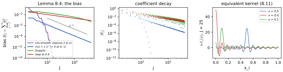
fig_8_S1. Download: PDF · SVGpp. 184–185 The bias is ignored from now on, and the target becomes \(r_n\), that is \(\th=(\th_1,\dots,\th_n)\). Its empirical coefficients are
\[ Z_j=\frac1n\sum_{i=1}^nY_i\,\phi_j(x_i),\qquad j=1,\dots,n, \tag{8.6} \]and, as in equation (7.15) of Chapter 7,
\[ Z_j\approx\N\Big(\th_j,\frac{\sigma^2}n\Big). \tag{8.7} \]What "\(\approx\)" means is exact enough to state: \(Z\) is Normal with mean \(n^{-1}\sum_ir(x_i)\phi_j(x_i)\) (a Riemann sum for \(\th_j\)), every variance is exactly \(\sigma^2/n\), and the correlations are at most \(2/n\), because \(n^{-1}\sum_i\phi_j(x_i)\phi_k(x_i)\) is 1 for \(j=k\) and \(0\), \(-2/n\) or \(-\sqrt2/n\) otherwise. On the midpoint grid \(x_i=(i-\tfrac12)/n\) the vectors \((\phi_j(x_i))_i\) are exactly orthogonal (the type II discrete cosine transform), and then the \(Z_j\) are exactly independent. Proofs: Probability and Statistical Inference, Filling the gap 21.9.
See also (companion course): Probability and Statistical Inference, Theorem 21.8 (the distribution of the coefficients).
The maximum likelihood estimator \(\hth=Z\) has risk \(n\cdot\sigma^2/n=\sigma^2\), which does not go to 0. The James–Stein estimator (7.41) does better by minimising estimated risk over the shrinkers \((bZ_1,\dots,bZ_n)\); react minimises over larger classes.
Definition (modulators) p. 185, (8.8)
A modulator is a vector \(b=(b_1,\dots,b_n)\) with \(0\le b_j\le1\); the modulation estimator is
\[ \hth=bZ=(b_1Z_1,\dots,b_nZ_n). \tag{8.8} \]The classes: constant modulators \((b,\dots,b)\) (\(\Mcons\)); nested subset selection modulators \((1,\dots,1,0,\dots,0)\) (\(\Mnss\)); monotone modulators \(1\ge b_1\ge\dots\ge b_n\ge0\) (\(\Mmon\)). Note \(\Mnss\subset\Mmon\) and \(\Mcons\subset\Mmon\).
Given \(b\), the function estimate is
\[ \hr(x)=\sum_{j=1}^n\hth_j\phi_j(x)=\sum_{j=1}^nb_jZ_j\phi_j(x), \tag{8.9} \]and substituting (8.6) shows that it is a linear smoother,
\[ \hr(x)=\sum_{i=1}^nY_i\,\ell_i(x), \tag{8.10} \] \[ \ell_i(x)=\frac1n\sum_{j=1}^nb_j\phi_j(x)\phi_j(x_i). \tag{8.11} \]Shrinking the high-frequency coefficients smooths the curve, so choosing \(b\) plays the role of choosing a bandwidth; here the choice is made by Stein's unbiased risk estimate (Section 7.4) instead of cross-validation.
p. 186 The risk of \(\hth=bZ\) is \(R(b)=\E_\th\sum_{j=1}^n(b_jZ_j-\th_j)^2\). It involves \(\sigma\), which has to be estimated. The book's estimator uses the last \(J_n\) coefficients; as printed, (8.12) reads \((n-J_n)^{-1}\sum_{i=n-J_n+1}^nZ_i^2\), which estimates \(J_n\sigma^2/(n(n-J_n))\), not \(\sigma^2\) (Notes on the book). The consistent version, used throughout these notes and the code, is
\[ \hs^2=\frac n{J_n}\sum_{j=n-J_n+1}^nZ_j^2 \tag{8.12} \]with the default \(J_n=n/4\). For the Doppler data of Figure 8.1 it gives \(\hs=0.0970\) (true value 0.1); the printed formula gives 0.0018.
Filling the gap 8.3: why the top coefficients contain only noise, and the consistency of (8.12) (Exercises 5 and 6) p. 186
Work on the midpoint grid, where the \(Z_j\) are exactly independent \(\N(\beta_j,\sigma^2/n)\) with \(\beta_j=n^{-1}\sum_ir(x_i)\phi_j(x_i)\) (on the grid \(i/n\) the same holds up to correlations of order \(1/n\)). Then
\[ \E\hs^2=\sigma^2+\frac n{J_n}\sum_{j\gt n-J_n}\beta_j^2,\qquad \V\hs^2=\frac{2\sigma^4}{J_n}+\frac{4\sigma^2n}{J_n^2}\sum_{j\gt n-J_n}\beta_j^2 . \]If \(r\) is absolutely continuous with \(\int_0^1r'^2\le c^2\), then
\[ \frac n{J_n}\sum_{j\gt n-J_n}\beta_j^2\le\frac{c^2}{4J_n\,n\,\sin^2\!\big(\pi(n-J_n)/(2n)\big)} . \]Hence \(\hs^2\to\sigma^2\) in mean square, uniformly over \(\{r:\int r'^2\le c^2\}\) (in the cosine basis this set is exactly the Sobolev ellipsoid \(\sum_j(\pi(j-1))^2\th_j^2\le c^2\), so this covers \(\Theta(m,c)\) for \(m\ge1\)), whenever \(J_n\to\infty\) and \(n-J_n\to\infty\): the two conditions of the book. With \(J_n=n/4\) the bias is at most \(c^2/(0.85\,n^2)\) and the standard deviation about \(\sigma^2\sqrt{8/n}\).
Proof
Moments. \(\E Z_j^2=\beta_j^2+\sigma^2/n\) and, for a Normal variable, \(\V Z_j^2=2(\sigma^2/n)^2+4\beta_j^2\sigma^2/n\). Sum the \(J_n\) independent terms and multiply by \(n/J_n\) (or its square).
The top coefficients see only differences. Let \(D\) be the \((n-1)\times n\) first-difference matrix, \((Dv)_i=v_{i+1}-v_i\). The vectors \(v_k=(\cos(k\pi(i-\tfrac12)/n))_{i=1}^n\), \(k=0,\dots,n-1\), are eigenvectors of \(D^\T D\) (the path-graph Laplacian with free ends) with eigenvalues \(\lambda_k=4\sin^2(k\pi/(2n))\): this is checked directly from the identity \(\cos(\alpha+h)+\cos(\alpha-h)=2\cos h\cos\alpha\) in the interior rows and from \(\cos(k\pi/(2n))=\cos(-k\pi/(2n))\) in the two end rows. They are orthogonal with \(\norm{v_k}^2=n/2\) for \(k\ge1\). Write \(\mathbf r=(r(x_i))_i\). Since \(\phi_j(x_i)=\sqrt2\,v_{j-1,i}\), we have \(\ip{\mathbf r}{v_{j-1}}^2/\norm{v_{j-1}}^2=n\beta_j^2\), and expanding \(\mathbf r\) in the eigenbasis,
\[ \norm{D\mathbf r}^2=\sum_k\lambda_k\frac{\ip{\mathbf r}{v_k}^2}{\norm{v_k}^2}\ \ge\ \lambda_{n-J_n}\sum_{j\gt n-J_n}n\beta_j^2 , \]because \(\lambda_k\) increases in \(k\). Finally, by Cauchy–Schwarz,
\[ (r(x_{i+1})-r(x_i))^2=(\int_{x_i}^{x_{i+1}}r')^2\le n^{-1}\int_{x_i}^{x_{i+1}}r'^2, \]so \(\norm{D\mathbf r}^2\le c^2/n\). Combine: \(\sum_{j\gt n-J_n}\beta_j^2\le c^2/(n^2\lambda_{n-J_n})\). Multiply by \(n/J_n\) to get the displayed bound. When \(n-J_n\to\infty\), \(\sin(\pi(n-J_n)/(2n))\ge(n-J_n)/n\), so the bias is at most \(c^2n/(4J_n(n-J_n)^2)\to0\); the variance \(2\sigma^4/J_n+\dots\to0\) when \(J_n\to\infty\). Both bounds depend on \(r\) only through \(c\): the convergence is uniform.
The Sobolev ellipsoid. For absolutely continuous \(r\), \(r'=-\sum_{k\ge1}\sqrt2\,k\pi\,\th_{k+1}\sin(k\pi x)\) in \(\Ltwo\) (integrate the sine series term by term), and \(\{\sqrt2\sin(k\pi x)\}\) is orthonormal and complete, so \(\int r'^2=\sum_{j\ge2}(\pi(j-1))^2\th_j^2\). No boundary condition is needed for one derivative.
Intuition. On the grid \(i/n\), \(\phi_{n-k+1}(i/n)=(-1)^i\phi_{k+1}(i/n)\): the top coefficients are alternating-sign sums, which cancel a smooth \(r\) and keep the noise, much like the difference-based variance estimators of Section 5.6. The same consistency argument, with the factor \(n/J_n\) included, is in Probability and Statistical Inference, Filling the gap 21.10. ∎
Theorem 8.13 (the risk of a modulator, and its estimate) p. 186, (8.14)–(8.15); Exercise 2
If the \(Z_j\) are independent \(\N(\th_j,\sigma^2/n)\), the risk of \(\hth=bZ\) is
\[ R(b)=\sum_{j=1}^n\th_j^2(1-b_j)^2+\frac{\sigma^2}n\sum_{j=1}^nb_j^2 . \tag{8.14} \]The (modified) SURE of \(R(b)\) is
\[ \Rh(b)=\sum_{j=1}^n\Big(Z_j^2-\frac{\hs^2}n\Big)_+(1-b_j)^2+\frac{\hs^2}n\sum_{j=1}^nb_j^2 , \tag{8.15} \]with \(\hs^2\) consistent, such as (8.12). Without the positive part and with \(\sigma\) known, the estimate \(\Rt(b)\) is unbiased: \(\E\Rt(b)=R(b)\) for every fixed \(b\).
Proof
\(b_jZ_j-\th_j=b_j(Z_j-\th_j)-(1-b_j)\th_j\). Square and take expectations: the cross term has mean 0 since \(\E(Z_j-\th_j)=0\), and \(\E(Z_j-\th_j)^2=\sigma^2/n\). So \(\E(b_jZ_j-\th_j)^2=b_j^2\sigma^2/n+(1-b_j)^2\th_j^2\); sum over \(j\) (independence is not even needed for the risk). For the estimate, \(\E Z_j^2=\th_j^2+\sigma^2/n\), so \(Z_j^2-\sigma^2/n\) is unbiased for \(\th_j^2\); replace each \(\th_j^2\) in (8.14) by it. This is SURE (Theorem 7.17) applied to \(\hth=bZ\): \(g_j=(b_j-1)Z_j\), \(D_j=b_j-1\), and (7.19) gives \(n\sigma_n^2+2\sigma_n^2\sum(b_j-1)+\sum(1-b_j)^2Z_j^2\), which rearranges to the same expression. ∎
Filling the gap 8.4: what the positive part does to the risk estimate p. 186, footnote 3
The footnote says the positive part "usually improves the risk estimate". It keeps every term non-negative, but it biases the level of \(\Rh\) upwards: since \(x\mapsto x_+\) is convex, Jensen's inequality gives \(\E(Z_j^2-s)_+\ge(\E Z_j^2-s)_+=\th_j^2\), and for a pure-noise coordinate (\(\th_j=0\), \(Z_j^2/s\sim\chi^2_1\))
\[ \E\big(Z_j^2-s\big)_+=s\,\E(\chi^2_1-1)_+=2\phi(1)\,s=0.484\,s . \]For the Doppler data about 840 of the 1000 coefficients are noise, so \(\Rh\) at the chosen \(J\) is about \(840\times0.484\times10^{-5}=0.004\) above the true risk: \(\Rh=0.0061\) against \(R=0.0025\) and \(\Rt=0.0026\). The choice of \(J\) for nested modulators is less affected: \(\Rh(J)-\Rh(J-1)=s-(Z_J^2-s)_+\) and \(\Rt(J)-\Rt(J-1)=2s-Z_J^2\) are negative for exactly the same \(J\) (when \(Z_J^2\gt 2s\)), a Mallows \(C_p\) rule for each coefficient, although the two curves can still have different minimisers. The same remarks for the companion course's estimator are in Probability and Statistical Inference, Filling the gap 21.5.
Derivation of \(2\phi(1)\)
For \(Z\sim\N(0,1)\),
\[ \E(Z^2-1)_+=2\int_1^\infty(z^2-1)\phi(z)\,\d z. \]Since \(z\phi(z)=-\phi'(z)\), integration by parts gives
\[ \int_1^\infty z^2\phi=\big[-z\phi\big]_1^\infty+\int_1^\infty\phi=\phi(1)+1-\Phi(1), \]and \(\int_1^\infty\phi=1-\Phi(1)\). The difference is \(\phi(1)\), so \(\E(Z^2-1)_+=2\phi(1)=0.4839\). ∎
Definition 8.16 (react) p. 187
Given a class \(\Mc\) of modulators, the modulation estimator is \(\hth=(\hat b_1Z_1,\dots,\hat b_nZ_n)\), where \(\hat b\) minimises \(\Rh(b)\) over \(\Mc\); the react function estimate is \(\hr(x)=\sum_j\hat b_jZ_j\phi_j(x)\).
Theorem 8.17 (Beran and Dümbgen, 1998) p. 187
Let \(\Mc\) be \(\Mcons\), \(\Mnss\) or \(\Mmon\), let \(b^*\) minimise the true risk \(R(b)\) over \(\Mc\) and \(\hat b\) the estimated risk. Then \(|R(\hat b)-R(b^*)|\to0\) as \(n\to\infty\). For \(\Mcons\) and \(\Mmon\), \(\hth=\hat bZ\) achieves the Pinsker bound (7.29).
Filling the gap 8.5: the uniform closeness of estimated and true risk, with a proof for nested and monotone modulators
The theorem rests on one fact: the estimated risk is close to the true risk uniformly over the class, so the minimiser of one nearly minimises the other. Here is a complete proof in the setting \(Z_j\sim\N(\th_j,s)\) independent, \(s=\sigma^2/n\) known, and the unbiased \(\Rt\):
\[ \E\sup_{b\in\Mmon}\big|\Rt(b)-R(b)\big|\le2\Big(\frac{2\sigma^4}n+\frac{4\sigma^2}n\norm{\th}^2\Big)^{1/2},\qquad 0\le R(\hat b)-R(b^*)\le2\sup_{b\in\Mc}|\Rt(b)-R(b)| , \]for \(\Mc=\Mnss\) or \(\Mmon\) and \(\hat b\) minimising \(\Rt\) over \(\Mc\). So \(R(\hat b)-R(b^*)=\OP(n^{-1/2})\), uniformly over \(\norm\th\le C\).
Proof
Reduction. \(\Rt(b)-R(b)=\sum_j\xi_j(1-b_j)^2\) with \(\xi_j=Z_j^2-s-\th_j^2=2\th_j\sqrt s\,\epsilon_j+s(\epsilon_j^2-1)\): independent, mean 0, \(\V\xi_j=4s\th_j^2+2s^2\). The coefficients \(w_j=(1-b_j)^2\) are non-decreasing in \(j\) and lie in \([0,1]\) when \(b\in\Mmon\). Any such sequence is a mixture of tail indicators: \(w_j=\sum_{J=0}^{n-1}\pi_J\,1\{j\gt J\}\) with \(\pi_0=w_1\), \(\pi_J=w_{J+1}-w_J\ge0\) and \(\sum_J\pi_J=w_n\le1\). Hence
\[ |\Rt(b)-R(b)|=\Big|\sum_J\pi_J\,T_J\Big|\le\max_{0\le J\lt n}|T_J|,\qquad T_J=\sum_{j\gt J}\xi_j . \]Maximal inequality. The tail sums \(T_{n-1},T_{n-2},\dots,T_0\) are partial sums of independent mean-zero variables taken from the end, so by Kolmogorov's (or Doob's \(L^2\)) maximal inequality
\[ \E\max_J T_J^2\le4\E T_0^2=4\sum_j\V\xi_j=4(2ns^2+4s\norm\th^2). \]Jensen's inequality gives the bound on \(\E\max|T_J|\), and \(ns^2=\sigma^4/n\), \(s=\sigma^2/n\).
Oracle inequality.
\[ R(\hat b)-R(b^*)=[R(\hat b)-\Rt(\hat b)]+[\Rt(\hat b)-\Rt(b^*)]+[\Rt(b^*)-R(b^*)]; \]the middle bracket is \(\le0\) because \(\hat b\) minimises \(\Rt\), and each outer bracket is at most the supremum. ∎
What this does not give. The minimax risk over \(\Theta(m,c)\) is of order \(n^{-2m/(2m+1)}\), which is smaller than \(n^{-1/2}\) when \(m\gt 1/2\); the bound above shows the difference vanishes, not that it is small relative to the risk. That stronger statement, and the Pinsker efficiency for \(\Mmon\) (whose minimiser over the ellipsoid is the Pinsker estimator of Chapter 7, a monotone modulator), need the sharper empirical-process bounds of Beran and Dümbgen (1998); with \(\hs\) estimated and the positive part, one adds the consistency of Filling the gap 8.3. The proof shows why the class must be small: for arbitrary modulators the coefficients \(w_j\) are no longer monotone, the reduction to \(n\) tail sums fails, and the supremum of \(|\Rt-R|\) is of order 1 (Exercise 12).
p. 187 Computing \(\hat b\). Over \(\Mcons\), the minimiser of \(\Rt\) is \(b=(1-n\hat s/\sum_jZ_j^2)_+\), the positive-part James–Stein factor (with \(n\) in place of \(n-2\)); the minimiser of \(\Rh\) with the positive part is \(S/(S+n\hat s)\), \(S=\sum_j(Z_j^2-\hat s)_+\). Over \(\Mnss\), compute
\[ \Rh(J)=\frac{J\hs^2}n+\sum_{j=J+1}^n\Big(Z_j^2-\frac{\hs^2}n\Big)_+ \tag{8.18} \]for every \(J\) and take the smallest (and plot it). Over \(\Mmon\), write
\[ \Rt(b)=\sum_{i=1}^n(b_i-g_i)^2Z_i^2+\frac{\hs^2}n\sum_{i=1}^ng_i,\qquad g_i=\frac{Z_i^2-\hs^2/n}{Z_i^2}, \tag{8.19} \]so that one minimises \(\sum_i(b_i-g_i)^2Z_i^2\) subject to \(b_1\ge\dots\ge b_n\): a weighted least squares problem with a monotonicity constraint, solved by the pooled-adjacent-violators (PAV) algorithm (Robertson, Wright and Dykstra 1988).
Filling the gap 8.6: equation (8.19), the PAV algorithm, and the constraint \(0\le b\le1\) (Exercise 3)
(a) (8.19) is an identity for the unbiased estimate \(\Rt\) (no positive part); with the positive part of (8.15) it is false in general. (b) PAV returns the weighted non-increasing least squares fit \(f\) of \(g\). (c) The monotone modulator is \(\hat b=\min(\max(f,0),1)\): clipping the unconstrained isotonic fit solves the problem with the box constraint as well. Our PAV implementation agrees with scikit-learn's isotonic regression to \(10^{-10}\), and the clipped solution agrees with a general constrained optimiser.
Proofs
(a) Write \(\hat s=\hs^2/n\) and expand, using \(g_iZ_i^2=Z_i^2-\hat s\):
\[ (b_i-g_i)^2Z_i^2+\hat sg_i=b_i^2Z_i^2-2b_i(Z_i^2-\hat s)+g_i(Z_i^2-\hat s)+\hat sg_i=b_i^2Z_i^2-2b_i(Z_i^2-\hat s)+(Z_i^2-\hat s), \]using \(g_i(Z_i^2-\hat s)+\hat sg_i=g_iZ_i^2\). On the other side,
\[ (Z_i^2-\hat s)(1-b_i)^2+\hat sb_i^2=(Z_i^2-\hat s)-2b_i(Z_i^2-\hat s)+b_i^2Z_i^2. \]They agree term by term. With \((Z_i^2-\hat s)_+\) in place of \(Z_i^2-\hat s\) the first expression no longer matches when \(Z_i^2\lt\hat s\).
Characterisation. Let \(K\) be the cone of non-increasing vectors and \(\ip uv_w=\sum_iw_iu_iv_i\) with \(w_i=Z_i^2\gt0\). The weighted projection \(f\) of \(g\) on the closed convex cone \(K\) is characterised by: \(f\in K\), \(\ip{f-g}f_w=0\) and \(\ip{f-g}c_w\ge0\) for all \(c\in K\). Every \(c\in K\) is \(c=c_n\mathbf 1+\sum_{k\lt n}(c_k-c_{k+1})\mathbf 1_{[1,k]}\) with non-negative increments, and \(\pm\mathbf1\in K\); so the conditions reduce to: the prefix sums \(P_k=\sum_{i\le k}w_i(f_i-g_i)\) are \(\ge0\) for all \(k\), \(P_n=0\), and \(\ip{f-g}f_w=0\).
(b) PAV. PAV scans left to right, keeps blocks of consecutive indices with value equal to the weighted mean of \(g\) on the block, and merges the last two blocks while their values increase. At the end the block values are non-increasing, so \(f\in K\); \(f\) is constant on blocks and \(\sum_{i\in B}w_i(f_i-g_i)=0\) on each block, which gives \(P_n=0\) and \(\ip{f-g}f_w=0\). For the prefix sums it suffices that every prefix \(B'\) of a block \(B\) has weighted mean of \(g\) at most the mean of \(B\) (then \(\sum_{i\in B'}w_i(f_i-g_i)=W_{B'}(\bar g_B-\bar g_{B'})\ge0\), and complete blocks contribute 0). This holds for single indices and is preserved by a merge: blocks \(A\), \(B\) are merged only when \(\bar g_A\lt\bar g_B\); a prefix inside \(A\) has mean \(\le\bar g_A\lt\bar g_{A\cup B}\), and a prefix \(A\cup B'\) has mean
\[ (W_A\bar g_A+W_{B'}\bar g_{B'})/(W_A+W_{B'})\le(W_A\bar g_A+W_{B'}\bar g_B)/(W_A+W_{B'})\le\bar g_{A\cup B}, \]because \(\bar g_{B'}\le\bar g_B\), \(W_{B'}\le W_B\) and \(\bar g_A\lt\bar g_B\).
(c) Clipping. Let \(\hat b=\min(\max(f,0),1)\) and let \(c\in K\cap[0,1]^n\). The objective \(F(b)=\sum_iw_i(b_i-g_i)^2\) is convex, so it suffices that \(\sum_iw_i(\hat b_i-g_i)(c_i-\hat b_i)\ge0\). Split \(\hat b-g=(f-g)+(\hat b-f)\). First, \(\ip{f-g}c_w\ge0\) by the characterisation, and \(\ip{f-g}{\hat b}_w=0\) because \(\hat b\) is constant on the blocks of \(f\) and \(f-g\) has zero weighted sum on each block. Second, \((\hat b_i-f_i)(c_i-\hat b_i)\ge0\) for each \(i\): it is 0 where \(0\le f_i\le1\); where \(f_i\gt1\), \(\hat b_i-f_i\lt0\) and \(c_i-1\le0\); where \(f_i\lt0\), \(\hat b_i-f_i\gt0\) and \(c_i\ge0\). ∎
Summary of react p. 188
- Compute \(Z_j=n^{-1}\sum_iY_i\phi_j(x_i)\) for \(j=1,\dots,n\), and \(\hs^2\) from (8.12).
- Find \(\hat J\) minimising \(\Rh(J)\) of (8.18).
- Estimate \(\hr(x)=\sum_{j=1}^{\hat J}Z_j\phi_j(x)\).
Monotone modulators usually give fits close to the nested ones, and the nested version is the simplest; the book recommends it as the default. Code: react, nss_risk, mon_modulator, const_modulator.
Example 8.20 (Doppler function) p. 188
\(r(x)=\sqrt{x(1-x)}\sin\big(2.1\pi/(x+0.05)\big)\), \(n=1000\), \(\sigma=0.1\), \(x_i=i/n\). On our sample (the same one as Figure 5.6), \(\hs=0.0970\) and the estimated risk (8.18) is smallest at \(\hat J=157\) (the book's sample: 187 terms kept, 813 dropped). The fit resolves the oscillations down to about \(x=0.05\) and is slightly rough on the smooth right half: like local linear regression with one bandwidth, one global \(J\) cannot suit both ends of a spatially inhomogeneous function.
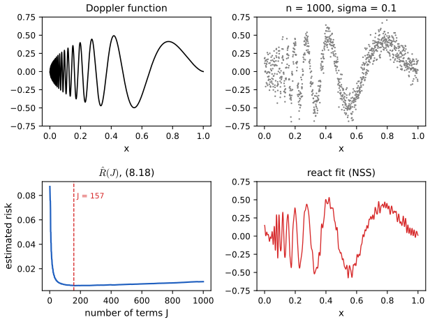
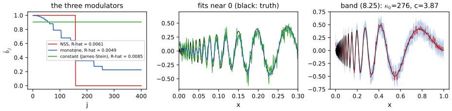
fig_8_S2. Download: PDF · SVGExample 8.21 (CMB data) p. 188
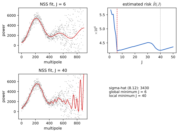
The 899 WMAP power-spectrum estimates (multipoles 2 to 900), treated as a regular design. The estimated risk of the nested modulator is smallest at \(J=6\), with a second local minimum at \(J=40\) whose estimated risk is only 0.5% larger. The 6-term fit is close to the local regression fits of Chapter 5; the 40-term fit follows the noise on the right, where the variance is largest. The constant-variance model is wrong here, as the book notes: \(\hs=3430\) averages a small noise level on the left and a very large one on the right.
pp. 188–189 Confidence sets. If \(B_n\) is a confidence ball for \(\th\in\R^n\) (Section 7.8), then
\[ C_n=\Big\{r=\sum_{j=1}^n\th_j\phi_j:\ (\th_1,\dots,\th_n)\in B_n\Big\} \tag{8.22} \]is a confidence ball for \(r_n\) (in \(\Ltwo\), by Parseval). The pivotal method of Section 7.8 gives the following.
Theorem 8.23 (Beran and Dümbgen, 1998) pp. 188–189, (8.24)
Let \(\hth\) be the monotone or nested react estimator and \(\hs^2\) the estimate (8.12). Let
\[ B_n=\Big\{\th\in\R^n:\ \sum_{j=1}^n(\hth_j-\th_j)^2\le s_n^2\Big\},\qquad s_n^2=\Rh(\hat b)+\frac{\hat\tau\,z_\alpha}{\sqrt n} , \tag{8.24} \]with \(\hat\tau\) an estimate of the standard deviation of \(\sqrt n\,(L-\Rh)\), \(L=\norm{\hth-\th}^2\). Then for any \(c\gt0\) and \(m\gt1/2\),
\[ \lim_n\sup_{\th\in\Theta(m,c)}|\P_\th(\th\in B_n)-(1-\alpha)|=0. \]The book's expression for \(\hat\tau^2\) leaves out part of the variability of \(\hs\); the variance derived below is the one used in these notes and the code (Notes on the book).
Filling the gap 8.7: the variance of the pivot, with the noise level estimated
Fix \(b\), let \(Z_j\sim\N(\th_j,s)\) independent with \(s=\sigma^2/n\), let \(\hat s=\hs^2/n\) with \(\hs^2\) from (8.12), so that \(\hat s=J_n^{-1}\sum_{j\in T}Z_j^2\) over the top block \(T\) of \(J_n\) coordinates, and let \(\Rt(b)\) be the unbiased risk estimate with \(\hat s\) in place of \(s\). Put \(A=\sum_k(2b_k-1)\) and \(c_j=1/J_n\) for \(j\in T\), 0 otherwise. If \(\th_j=0\) on \(T\), then \(\E(L-\Rt)=0\) and
\[ \V\big(L-\Rt\big)=2s^2\sum_{j=1}^n\big((2b_j-1)-Ac_j\big)^2+4s\sum_{j=1}^n\th_j^2\big((1-b_j)+Ac_j\big)^2 , \]estimated by putting \(Z_j^2-\hat s\) for \(\th_j^2\). The terms with \(A\) come from the error in \(\hat s\); since a nested fit has \(b_j=0\) for most \(j\), \(A\approx2\hat J-n\) is of order \(-n\), and these terms are not small. In the book's expression \(A\) is replaced by \(2b_j-1\). With \(b\) fixed at \(J=150\) on the Doppler model, the derived standard deviation matches 1500 simulations within 1.3%, and the printed one is 16% too small. With \(\sigma\) known (\(c_j=0\)), both reduce to the formula \(\tau^2=2n\sigma_n^2(n\sigma_n^2+2\sum_{j\gt m}\th_j^2)\) of Section 7.8.
Derivation
Write \(Z_j=\th_j+\sqrt s\,\epsilon_j\). Then
\[ L=\sum_j\big((b_j-1)\th_j+b_j\sqrt s\epsilon_j\big)^2 \]and
\[ \Rt=\sum_j(Z_j^2-\hat s)(1-b_j)^2+\hat s\sum_jb_j^2=\sum_j Z_j^2(1-b_j)^2+\hat s A, \]since \(\sum_j\{b_j^2-(1-b_j)^2\}=\sum_j(2b_j-1)=A\). Expanding the squares, the \(\th_j^2(1-b_j)^2\) terms cancel and
\[ L-\Rt=-2\sqrt s\sum_j\th_j(1-b_j)\epsilon_j+s\sum_j\big(b_j^2-(1-b_j)^2\big)\epsilon_j^2-\hat sA . \]With \(\th=0\) on \(T\), \(\hat s=s\sum_jc_j\epsilon_j^2\), so the last two terms combine into \(s\sum_j\{(2b_j-1)-Ac_j\}\epsilon_j^2\), whose mean is \(s\{A-A\}=0\). The linear and quadratic parts are uncorrelated (\(\E\epsilon^3=0\)), \(\V\epsilon_j=1\), \(\V\epsilon_j^2=2\), and the coordinates are independent, which gives the variance with \(Ac_j=0\) in the second sum. If \(\th\ne0\) on \(T\), \(\hat s\) also contains \(J_n^{-1}\sum_T(\th_j^2+2\sqrt s\th_j\epsilon_j)\): this adds the linear coefficients \(-2\sqrt s\,\th_jAc_j\) (hence the \(+Ac_j\) in the second sum) and a bias \(-A J_n^{-1}\sum_T\th_j^2\), which is small exactly when \(\hs\) is consistent (Filling the gap 8.3). As the sum of \(n\) independent terms, none dominant, \((L-\Rt)/\sqrt{\V}\) is asymptotically Normal (Lyapunov), so \(\P(L\le\Rt+z_\alpha\sqrt{\V})\to1-\alpha\) for fixed \(b\).
With \(\hat b\) chosen from the data, the minimum of \(\Rt\) is biased downwards, so the pivot is shifted to the right: in 1000 simulations of the Doppler model with the nested modulator, the ball with the derived variance covered \(\th\) in 87.5% of cases and the printed one in 83.2% (nominal 95%; Figure 8.S3). The uniform statement of the theorem is asymptotic and controls this shift through the uniform bound of Filling the gap 8.5; at \(n=1000\) the Doppler function, far from smooth near 0, is a hard case. ∎
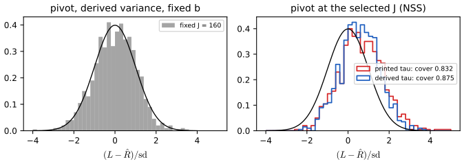
fig_8_S3, ball_coverage. Download: PDF · SVGp. 189 Bands. Since \(\hr\) is a linear smoother, the band of Section 5.7, (5.99), applies:
\[ I(x)=\Big(\hr(x)-c\,\hs\norm{\ell(x)},\ \hr(x)+c\,\hs\norm{\ell(x)}\Big), \tag{8.25} \] \[ \norm{\ell(x)}^2\approx\frac1n\sum_{j=1}^nb_j^2\phi_j^2(x), \tag{8.26} \]with \(c\) from the tube formula (5.102). Like every band of Chapter 5, it covers the mean of the estimator, here \(\sum_jb_j\E(Z_j)\phi_j\), not \(r\).
Filling the gap 8.8: equation (8.26), and the variance at the end points (Exercise 4)
Exactly, with \(G_{jk}=n^{-1}\sum_i\phi_j(x_i)\phi_k(x_i)\),
\[ \norm{\ell(x)}^2=\frac1n\sum_{j,k}b_jb_k\phi_j(x)\phi_k(x)G_{jk}. \]So (8.26) is exact when \(G=I\) (the midpoint grid, or an irregular design after Gram–Schmidt), and on the grid \(i/n\), where \(|G_{jk}-\delta_{jk}|\le2/n\), the error is at most \(2n^{-2}(\sum_j b_j|\phi_j(x)|)^2\). For the 157-term Doppler fit the relative error of \(\norm{\ell(x)}\) is at most 9%, near the end points. For a nested modulator, (8.26) is \(n^{-1}\big(J+\sum_{k=1}^{J-1}\cos(2k\pi x)\big)\): about \(J/n\) inside the interval and exactly \((2J-1)/n\) at \(x=0\) and \(x=1\). The variance doubles at the end points, the price of the reflection in Filling the gap 8.12.
Proof
\[ \norm{\ell(x)}^2=\sum_i\ell_i(x)^2=n^{-2}\sum_i\big(\sum_jb_j\phi_j(x)\phi_j(x_i)\big)^2=n^{-2}\sum_{j,k}b_jb_k\phi_j(x)\phi_k(x)\sum_i\phi_j(x_i)\phi_k(x_i), \]which is the display. The error bound:
\[ |\sum_{j,k}b_jb_k\phi_j\phi_k(G_{jk}-\delta_{jk})|\le\frac2n\big(\sum_jb_j|\phi_j(x)|\big)^2. \]For the end points, \(\phi_j^2(x)=1+\cos(2(j-1)\pi x)\) for \(j\ge2\), so \(\sum_{j\le J}\phi_j^2(x)=J+\sum_{k=1}^{J-1}\cos(2k\pi x)\), which equals \(2J-1\) at \(x\in\{0,1\}\) and is \(J+O(1/\sin(\pi x))\) inside (a Dirichlet sum). The band's \(c\) comes from the tube formula exactly as in Filling the gap 5.16, with \(\kappa_0\) computed from the weights (8.11). ∎
See also: Chapter 5, Filling the gap 5.16 (the tube formula) and the tube formula demo; Probability and Statistical Inference, Theorem 21.11 (a cruder band for a fixed \(J\)).
8.3 Irregular Designs
pp. 189–190 For an irregular design, use a basis that is orthonormal for the empirical distribution \(P_n=n^{-1}\sum_i\delta_{x_i}\), with
\[ \ip fg=\int fg\,\d P_n=\frac1n\sum_{i=1}^nf(x_i)g(x_i),\qquad \norm f^2=\frac1n\sum_{i=1}^nf^2(x_i). \]Starting from convenient functions \(g_1,g_2,\dots\) (here the cosines at the rescaled design), Gram–Schmidt gives \(\phi_1=g_1/\norm{g_1}\) and, for \(r\ge2\), \(\phi_r=\psi_r/\norm{\psi_r}\) with \(\psi_r=g_r-\sum_{j\lt r}a_{r,j}\phi_j\), \(a_{r,j}=\ip{g_r}{\phi_j}\). Then
\[ Z_j=\frac1n\sum_{i=1}^nY_i\,\phi_j(x_i),\qquad j=1,\dots,n, \tag{8.27} \]and \(Z_j\approx\N(\th_j,\sigma^2/n)\), so everything above applies.
Filling the gap 8.9: Gram–Schmidt for the empirical measure, what is estimated, ties, and the noise level
- Exact orthonormality and independence. The \(\phi_j\) are orthonormal for \(P_n\) by induction; equivalently, the matrix \(\Phi=(\phi_j(x_i))\) satisfies \(\Phi^\T\Phi/n=I\) (it is \(\sqrt n\) times the \(Q\) of a QR decomposition of \((g_j(x_i))\)). So \(\Cov(Z)=\sigma^2n^{-2}\Phi^\T\Phi=(\sigma^2/n)I\) exactly, and with Normal errors the \(Z_j\) are exactly independent \(\N(\th_j,\sigma^2/n)\), where now \(\th_j=\ip r{\phi_j}=n^{-1}\sum_ir(x_i)\phi_j(x_i)\). Nothing is approximated, but the target changes: by the discrete Parseval relation the loss is \(\sum_j(\hth_j-\th_j)^2=n^{-1}\sum_i(\hr(x_i)-r(x_i))^2\), the average squared error at the design points.
- How many functions. \(\Ltwo(P_n)\) has dimension equal to the number of distinct \(x_i\), so with ties at most that many \(\phi_j\) exist; numerically, high-order cosines on clustered data are nearly dependent. The code orthonormalises at most \(n/2\) cosines and stops at the first one whose remaining norm is below \(10^{-3}\) of its original norm (glass data: 48 functions; motorcycle: 47). The \(\phi_j\) are functions, not only vectors: \(\phi(x)=g(x)R^{-1}\) with the triangular \(R\) of the decomposition, which is how fits and bands are drawn between the design points.
- The noise level. Complete the \(q\) functions by any orthonormal basis of the rest of \(\R^n\); those \(n-q\) coordinates have mean \(\approx0\) when \(r\) is captured by the first \(q\) functions, and the sum of their squares is \(\mathrm{RSS}_q/n\), the residual sum of squares after regressing \(Y\) on all \(q\) functions. When \(n-q\ge J_n\), (8.12) on these coordinates is the familiar \(\hs^2=\mathrm{RSS}_q/(n-q)\). The nested risk estimate is \[ J\hat s+\sum_{J\lt j\le q}(Z_j^2-\hat s)_++(\mathrm{RSS}_q/n-(n-q)\hat s)_+ \] .
Proof of orthonormality
Suppose \(\phi_1,\dots,\phi_{r-1}\) are orthonormal. Then
\[ \ip{\psi_r}{\phi_k}=\ip{g_r}{\phi_k}-\sum_{j\lt r}a_{r,j}\ip{\phi_j}{\phi_k}=a_{r,k}-a_{r,k}=0 \]for \(k\lt r\), and \(\norm{\psi_r}\gt0\) as long as \(g_r\) is not in the span of \(g_1,\dots,g_{r-1}\) at the design points; dividing by the norm gives a unit vector. In floating point the classical recursion loses orthogonality when columns are nearly dependent; the code subtracts the projections one at a time and repeats the sweep once ("twice is enough"), which restores orthogonality to rounding level (checked against numpy's Householder QR). ∎
See also (companion course): Probability and Statistical Inference, Filling the gap 21.12 (designs that are not equally spaced).
8.4 Density Estimation
p. 191 Let \(X_1,\dots,X_n\) be iid with density \(f\in\Ltwo(0,1)\), \(f=\sum_j\th_j\phi_j\). The coefficients are expectations, so
\[ Z_j=\frac1n\sum_{i=1}^n\phi_j(X_i),\qquad j=1,\dots,n, \tag{8.28} \]has \(\E Z_j=\int\phi_jf=\th_j\) and \(\V Z_j=n^{-1}\big(\int\phi_j^2f-\th_j^2\big)\equiv\sigma_j^2\). With \(\th_j=0\) for \(j\gt n\) and a modulation estimator \(\hth=bZ\), the risk is
\[ R(b)=\sum_{j=1}^nb_j^2\sigma_j^2+\sum_{j=1}^n(1-b_j)^2\th_j^2 . \tag{8.29} \]With \(\hat\sigma_j^2=n^{-2}\sum_i(\phi_j(X_i)-Z_j)^2\) and \(\th_j^2\) estimated by \(Z_j^2-\hat\sigma_j^2\),
\[ \Rh(b)=\sum_{j=1}^nb_j^2\hat\sigma_j^2+\sum_{j=1}^n(1-b_j)^2\big(Z_j^2-\hat\sigma_j^2\big)_+ , \tag{8.30} \]minimised over a class of modulators.
Filling the gap 8.10: the risk (8.29) and what (8.30) estimates
(a) (8.29) holds exactly, without Normality or independence of the \(Z_j\). (b) For the cosine basis \(\phi_j^2=1+\phi_{2j-1}/\sqrt2\) (\(j\ge2\)), so \(\sigma_j^2=n^{-1}(1+\th_{2j-1}/\sqrt2-\th_j^2)\le2/n\), and \(\sigma_1^2=0\) because \(Z_1=\th_1=1\). (c) \(\E\hat\sigma_j^2=(1-1/n)\sigma_j^2\) and \(\E(Z_j^2-\hat\sigma_j^2)=\th_j^2+\sigma_j^2/n\): before the positive part, the estimate of each term is biased by a factor or term of relative order \(1/n\). (d) Unlike regression, the \(Z_j\) are correlated (\(\Cov(Z_j,Z_k)=n^{-1}(\int\phi_j\phi_kf-\th_j\th_k)\)), which does not affect the risk but matters for confidence sets.
Proof
(a)
\[ \E(b_jZ_j-\th_j)^2=b_j^2\V Z_j+(b_j\E Z_j-\th_j)^2=b_j^2\sigma_j^2+(1-b_j)^2\th_j^2, \]using only \(\E Z_j=\th_j\); sum over \(j\); only the variance of each coordinate enters, so correlations between coordinates do not matter. (b) \(2\cos^2u=1+\cos2u\) with \(u=(j-1)\pi x\), and \(\sqrt2\cos(2(j-1)\pi x)=\phi_{2j-1}(x)\); \(|\th_{2j-1}|\le\sqrt2\) since \(|\phi|\le\sqrt2\) and \(\int f=1\). (c) \(n\hat\sigma_j^2\) is the sample variance with divisor \(n\) of the iid \(\phi_j(X_i)\), whose mean is \((n-1)/n\) times \(\V\phi_j(X)=n\sigma_j^2\); and \(\E Z_j^2=\th_j^2+\sigma_j^2\). (d) \(\Cov(Z_j,Z_k)=n^{-1}\Cov(\phi_j(X),\phi_k(X))\). The companion course proves the same facts for a fixed number of terms in Theorems 21.4 and 21.5. ∎
The estimate can be negative. Surgery removes the negative part and renormalises to integrate to 1; better repairs are in Glad, Hjort and Ushakov (2003).
Filling the gap 8.11: surgery never makes the error larger than a constant times the original error
Let \(\hat f^+=\max(\hat f,0)\), \(m=\int\hat f^+\) and \(f^*=\hat f^+/m\). Then \(\norm{\hat f^+-f}\le\norm{\hat f-f}\) pointwise in the integrand (where \(\hat f\lt0\), \(|0-f|=f\le f-\hat f\)), and \(\norm{f^*-f}\le(1+\norm{\hat f^+})\norm{\hat f-f}\) because \(m-1=\int_{\{\hat f\lt0\}}(-\hat f)\le\norm{\hat f-f}\) when \(\int\hat f=1\) (true for the cosine estimator, since \(Z_1=1\) and \(\int\phi_j=0\) for \(j\ge2\)). Full proof: Probability and Statistical Inference, Filling the gap 21.7. In all six cases of Exercise 11 surgery lowered the integrated squared error.
8.5 Comparison of Methods
p. 192 Local regression, splines and orthogonal series behave much alike: each has a bias–variance tradeoff governed by one smoothing parameter, and differences between them are rarely large relative to the width of the confidence bands. Local polynomials correct boundary bias automatically; orthogonal series can be modified to do so (Efromovich 1999); orthogonal series turn the problem into normal means, which is convenient for theory. Formally, an orthogonal series estimator is a kernel estimator with a particular kernel and conversely (Härdle, Kerkyacharian, Picard and Tsybakov 1998).
Filling the gap 8.12: the cosine series estimator is a kernel smoother with a reflected kernel
For the nested modulator with \(J\) terms, (8.11) is \(\ell_i(x)=n^{-1}K_J(x,x_i)\) with
\[ K_J(x,y)=\sum_{j=1}^J\phi_j(x)\phi_j(y)=D_J(x-y)+D_J(x+y),\qquad D_J(t)=\frac12+\sum_{k=1}^{J-1}\cos(k\pi t)=\frac{\sin\big((J-\frac12)\pi t\big)}{2\sin(\pi t/2)} . \]\(D_J\) is a Dirichlet kernel: a peak of height \(J-\frac12\) and width about \(2/J\) at \(t=0\), with slowly decaying ripples of both signs. So: (i) the bandwidth is \(h\approx1/J\), and \(J\asymp n^{1/5}\) corresponds to \(h\asymp n^{-1/5}\); (ii) the ripples (negative weights) cause the Gibbs overshoot at jumps; smoother modulators (monotone, or tapers such as \(b_j=1-j/J\), the Fejér kernel) damp them; (iii) the second term \(D_J(x+y)\) is the kernel centred at the mirror image \(-x\): the estimator smooths the data reflected about 0 (and about 1). Reflection keeps the weights summing to 1 near the boundary (no loss of mass, unlike a plain kernel average) but forces \(\hr'(0)=\hr'(1)=0\), so the bias at the ends is of order \(|r'(0)|/J\) rather than the \(O(h^2)\) of local linear regression (Theorem 5.65), and at \(x=0\) the two kernels coincide, doubling the variance (Filling the gap 8.8).
Derivation
For \(j\ge2\), with \(k=j-1\),
\[ \phi_j(x)\phi_j(y)=2\cos(k\pi x)\cos(k\pi y)=\cos(k\pi(x-y))+\cos(k\pi(x+y)), \]and \(\phi_1\phi_1=1=\frac12+\frac12\). Summing over \(j\le J\) gives \(D_J(x-y)+D_J(x+y)\). For the closed form, multiply \(D_J(t)\) by \(2\sin(\pi t/2)\) and use \(2\sin a\cos b=\sin(a+b)-\sin(b-a)\): the sum telescopes to \(\sin((J-\frac12)\pi t)\). Since \(\int_0^1\phi_j=0\) for \(j\ge2\), \(\int_0^1K_J(x,y)\,\d y=1\) for every \(x\), and \(n^{-1}\sum_iK_J(x,x_i)\approx1\) on a fine grid. Finally \(\phi_j'(x)=-\sqrt2(j-1)\pi\sin((j-1)\pi x)\) vanishes at 0 and 1 for every \(j\), so every finite cosine series has zero slope at the ends. ∎
8.6 Tensor Product Models
pp. 192–193 For a function of two variables on \([0,1]^2\), if \(\phi_0,\phi_1,\dots\) is an orthonormal basis of \(\Ltwo(0,1)\) (here indexed from 0, with \(\phi_0=1\)), the products \(\phi_{j,k}(x_1,x_2)=\phi_j(x_1)\phi_k(x_2)\) form an orthonormal basis of \(\Ltwo([0,1]^2)\), the tensor product basis, and
\[ r(x_1,x_2)=\beta_0+\sum_{j\ge1}\beta_{j,0}\phi_j(x_1)+\sum_{k\ge1}\beta_{0,k}\phi_k(x_2)+\sum_{j,k\ge1}\beta_{j,k}\phi_j(x_1)\phi_k(x_2), \]an ANOVA-like decomposition into a mean, two main effects and an interaction. Stronger smoothness assumptions on the interaction give better rates (Lin 2000; Wahba, Wang, Gu, Klein and Klein 1995; Gao, Wahba, Klein and Klein 2001; Lin, Wahba, Xiang, Gao, Klein and Klein 2000).
Filling the gap 8.13: the tensor product basis is orthonormal and complete; the ANOVA pieces; the cost in \(d\) dimensions
(a) Orthonormality and completeness in \(\Ltwo([0,1]^2)\). (b) With \(\phi_0=1\), the main effect \(\sum_j\beta_{j,0}\phi_j(x_1)\) equals \(\int r(x_1,x_2)\,\d x_2-\beta_0\), the interaction integrates to 0 in each variable separately, and the four pieces are mutually orthogonal. (c) Keeping \(J\) functions per coordinate in \(d\) dimensions costs \(J^d\sigma^2/n\) in variance; with bias \(O(J^{-2m})\) per coordinate the best \(J\asymp n^{1/(2m+d)}\) gives the rate \(n^{-2m/(2m+d)}\): the curse of dimensionality of Section 4.5. An additive model (main effects only) costs \(dJ\sigma^2/n\) and keeps the one-dimensional rate.
Proof
(a) By Fubini, \(\ip{\phi_{j,k}}{\phi_{j',k'}}=\ip{\phi_j}{\phi_{j'}}\ip{\phi_k}{\phi_{k'}}=\delta_{jj'}\delta_{kk'}\). For completeness, let \(f\in\Ltwo([0,1]^2)\) be orthogonal to every product. By Fubini, \(f(x_1,\cdot)\in\Ltwo(0,1)\) for almost every \(x_1\), and \(h_k(x_1)=\int f(x_1,x_2)\phi_k(x_2)\,\d x_2\) is in \(\Ltwo(0,1)\) (Cauchy–Schwarz) with \(\ip{h_k}{\phi_j}=\ip f{\phi_{j,k}}=0\) for all \(j\); completeness in one variable gives \(h_k=0\) almost everywhere. So for almost every \(x_1\), \(f(x_1,\cdot)\) is orthogonal to every \(\phi_k\), hence 0 in \(\Ltwo\); then \(\norm f^2=\int\!\!\int f^2=0\). (b) Integrate the expansion over \(x_2\): every term with \(k\ge1\) vanishes since \(\int\phi_k=0\). Orthogonality of the pieces is (a). (c) There are \(J^d\) coefficients each of variance \(\sigma^2/n\); for the bias, a function in a product Sobolev class has \(\sum\beta^2\) outside the \(J^d\) cube of order \(dJ^{-2m}\); balance \(J^d/n\) against \(J^{-2m}\). ∎
8.7 Bibliographic Remarks
p. 193 React is developed in Beran (2000) and Beran and Dümbgen (1998); Efromovich (1999) gives a different orthogonal series approach. The confidence sets are extended to non-constant variance by Genovese, Miller, Nichol, Arjunwadkar and Wasserman (2004), to wavelets by Genovese and Wasserman (2005), and to density estimation by Jang, Genovese and Wasserman (2004).
Notes on the book
The book's website has no errata list. Each point below gives its evidence: a derivation in these notes or a computation.
Page 184, footnote 2: the Sobolev ellipsoid is Definition 7.10
The footnote refers to "Definition 7.2"; Sobolev ellipsoids \(\Theta(m,c)\) are defined in Definition 7.10 (and the ellipsoid in (7.9)).
Page 186, (8.12): the noise estimate needs the factor \(n/J_n\)
As printed, \(\hs^2=(n-J_n)^{-1}\sum_{i=n-J_n+1}^nZ_i^2\) has \(J_n\) terms each of mean about \(\sigma^2/n\), so it estimates \(J_n\sigma^2/(n(n-J_n))\), which tends to 0. The displayed check below it ("\(\E\hs^2\approx\sigma^2\)") does not hold for the formula as printed. The consistent estimator is \(\hs^2=(n/J_n)\sum_{j=n-J_n+1}^nZ_j^2\) (Filling the gap 8.3), which is also the companion book's (21.26). On the Doppler data: 0.0970 against 0.0018 for \(\sigma=0.1\).
Pages 186–187: the constant modulator and equation (8.19)
"Minimizing \(\Rh(b)\) over \(\Mcons\) yields the James–Stein estimator" holds for the unbiased estimate \(\Rt\), where the minimiser is the positive-part factor \(1-n\hat s/\sum Z_j^2\) (with \(n\) instead of the James–Stein \(n-2\)); with the positive part of (8.15) the minimiser is \(S/(S+n\hat s)\), \(S=\sum(Z_j^2-\hat s)_+\). Likewise (8.19) is an identity for \(\Rt\), not for \(\Rh\) of (8.15) (Filling the gap 8.6).
Pages 188–189, Theorem 8.23: the variance \(\tau^2\)
In the expression for \(\hat\tau^2\), the terms that account for the estimation of \(\sigma\) by (8.12) have \((2b_j-1)c_j\) where the derivation gives \(A\,c_j\) with \(A=\sum_k(2b_k-1)\) (the error in \(\hat s\) multiplies the whole sum \(\sum_k(2b_k-1)\) in the risk estimate, not one coordinate). Filling the gap 8.7 derives the variance; at a fixed nested modulator on the Doppler model, the derived standard deviation is within 1.3% of a simulation of 1500 data sets and the printed one 16% too small, and with \(\hat J\) chosen from the data the printed ball covers 83% instead of 88% (nominal 95%).
Page 190: \(\norm{\phi_j}=1\), and the starting functions
The normalisation should read \(\norm{\phi_j}=1\) (not \(\norm{\phi_j^2}=1\)). The \(g_1,\dots,g_n\) must be functions (so that \(\hr(x)\) can be evaluated off the design), linearly independent at the design points; "any convenient orthonormal basis for \(\R^n\)" only gives vectors, and an orthonormal basis of \(\R^n\) would already be orthonormal for \(P_n\) after scaling by \(\sqrt n\). With ties there are at most as many functions as distinct design points (Filling the gap 8.9).
Page 195, Exercise 13: the design \(x_{1i}=x_{2i}=i/n\) cannot identify a function of two variables
With both covariates equal, only \(t\mapsto r(t,t)\) is identifiable and the tensor product design matrix is singular (rank 5 instead of 9 for \(J_1=J_2=3\)). The solution below uses independent uniform covariates, presumably what is intended.
8.8 Exercises
All 14 exercises of Chapter 8 (pp. 193–195), restated in my own words, with complete solutions (hidden). Computational solutions use the chapter's code.
Exercise 8.1. Prove Lemma 8.4.
Solution
See Filling the gap 8.1: \(\sum_{j\gt n}\th_j^2\le c^2/\min_{j\gt n}a_j^2=O(n^{-2m})\), attained by putting all the mass of the ellipsoid on coordinate \(n+1\).
Exercise 8.2. Prove Theorem 8.13.
Solution
See the proof under Theorem 8.13: \(\E(b_jZ_j-\th_j)^2=b_j^2\sigma^2/n+(1-b_j)^2\th_j^2\), and \(Z_j^2-\sigma^2/n\) is unbiased for \(\th_j^2\). The effect of the positive part and of an estimated \(\sigma\) is in Filling the gap 8.4.
Exercise 8.3. Prove equation (8.19).
Solution
Expand both sides (Filling the gap 8.6, part (a)): both equal \(\sum_i\{b_i^2Z_i^2-2b_i(Z_i^2-\hat s)+(Z_i^2-\hat s)\}\). The identity holds for the risk estimate without the positive part; that is the version the monotone modulator minimises.
Exercise 8.4. Prove equation (8.26).
Solution
\(\norm{\ell(x)}^2=n^{-1}\sum_{j,k}b_jb_k\phi_j(x)\phi_k(x)G_{jk}\) with \(G=n^{-1}\Phi^\T\Phi\); (8.26) is the case \(G=I\), exact on the midpoint grid and accurate to \(O(1/n)\) entrywise on the grid \(i/n\) (Filling the gap 8.8).
Exercise 8.5. Show that the estimator (8.12) is consistent.
Solution
With the factor \(n/J_n\): \(\E\hs^2=\sigma^2+(n/J_n)\sum_{j\gt n-J_n}\beta_j^2\) and \(\V\hs^2=2\sigma^4/J_n+(4\sigma^2n/J_n^2)\sum_{j\gt n-J_n}\beta_j^2\). The variance tends to 0 when \(J_n\to\infty\); the bias tends to 0 when \(n-J_n\to\infty\), because the top coefficients of a function with \(\int r'^2\lt\infty\) are bounded through its first differences (Filling the gap 8.3). Mean-square convergence implies convergence in probability. A simulation with 20,000 replicates confirms both moment formulas.
Exercise 8.6. Show that (8.12) is uniformly consistent over Sobolev ellipsoids.
Solution
Case \(m\ge1\). Write
\[ \Delta_n=\frac n{J_n}\sum_{j\gt n-J_n}\beta_j^2 \]for the bias. Over \(\{r:\int r'^2\le c^2\}\), which in the cosine basis is the ellipsoid \(\sum_j(\pi(j-1))^2\th_j^2\le c^2\), Filling the gap 8.3 gives \(\Delta_n\le\bar\Delta_n=c^2n/(4J_n(n-J_n)^2)\) and
\[ \E(\hs^2-\sigma^2)^2=\Delta_n^2+\V\hs^2\le\bar\Delta_n^2+2\sigma^4/J_n+4\sigma^2\bar\Delta_n/J_n. \]The right side depends only on \(c\) and tends to 0, and Chebyshev's inequality gives \(\sup_\th\P(|\hs^2-\sigma^2|\gt\varepsilon)\to0\).
Case \(1/2\lt m\lt1\), on the midpoint grid, through aliasing. For \(l\gt n\) write \(l-1=2qn\pm k\) with \(0\le k\le n\); since
\[ \cos\big((2qn\pm k)\pi(i-\frac12)/n\big)=(-1)^q\cos\big(k\pi(i-\frac12)/n\big), \]the vector \((\phi_l(x_i))_i\) equals \(\pm\phi_{k+1}(x_i)\) up to a factor at most \(\sqrt2\) (and is 0 when \(k=n\)). Hence \(\beta_j=\th_j+\sum_{l\in A_j}\pm c_l\th_l\), \(|c_l|\le\sqrt2\), where the alias set \(A_j\) contains at most two indices \(l\gt(2q-1)n\) for each \(q\ge1\). By Cauchy–Schwarz,
\[ \Big(\sum_{l\in A_j}|c_l\th_l|\Big)^2\le2\Big(\sum_{l\in A_j}a_l^2\th_l^2\Big)\Big(\sum_{l\in A_j}a_l^{-2}\Big),\qquad \sum_{l\in A_j}a_l^{-2}\le C\sum_{q\ge1}\big((2q-1)n\big)^{-2m}=O(n^{-2m}), \]where the series converges because \(2m\gt1\). The alias sets are disjoint, so
\[ \sum_j(\beta_j-\th_j)^2=O(n^{-2m})\sum_la_l^2\th_l^2=O(c^2n^{-2m}), \]and \(\sum_{j\gt n-J_n}\th_j^2\le c^2/a_{n-J_n}^2=O(n^{-2m})\) when \(J_n=n/4\) (Lemma 8.4). So \(\Delta_n=(n/J_n)\,O(c^2n^{-2m})\to0\) uniformly, and the variance bound is as before. This is where \(m\gt1/2\) enters.
Exercise 8.7. Glass fragments: regress refractive index on aluminium content with react and with local linear smoothing; estimate the variance; give 95 percent bands.
Solution
Method: the design (214 fragments, many ties) is irregular, so the cosines at the rescaled aluminium values are orthonormalised for \(P_n\) (Filling the gap 8.9): 48 functions survive. The other coordinates give \(\hs=2.41\) (Rice's difference estimator: 2.46; the local linear residual estimator (5.86): 2.56). The estimated risk is almost flat beyond \(J=10\) and its global minimum is at \(J=39\), driven by a few outlying fragments; searching \(J\le\sqrt n=14\) (the restriction of Probability and Statistical Inference, Filling the gap 21.6) gives \(J=10\). Local linear: cross-validated \(h=0.528\).
method tuning \(\hs\) \(\kappa_0\) \(c\) react (NSS) J = 10 2.41 16.3 3.06 local linear h = 0.528 2.56 12.0 2.97 The two fits agree closely (Figure 8.S4): a rise to about 5 near aluminium 0.75, a fall to about 0 by 1.2, a plateau and a decline beyond 2.5. The react band is a little wider at the extremes, where the reflected kernel doubles the variance.
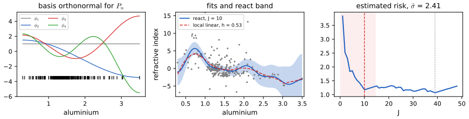
Figure 8.S4 (supplementary). Exercise 7. Left: \(\phi_1,\dots,\phi_4\) after Gram–Schmidt for the glass design. Middle: react (\(J=10\)) with its 95% band, and local linear regression. Right: estimated risk; the shaded range is \(J\le\sqrt n\). Not a figure of the book. Code: fig_8_S4. Download: PDF · SVGExercise 8.8. Motorcycle data (acceleration against time after impact): fit by react, give a 95 percent band and a 95 percent confidence ball, and find a way to display the ball.
Solution
The website's file has \(n=94\) observations at 94 distinct times. Gram–Schmidt keeps \(q=47\) functions; the remaining 47 coordinates give \(\hs=23.7\) (Rice: 23.9). The nested modulator keeps \(J=9\) functions; the band (8.25) has \(\kappa_0=14.6\) and \(c=3.03\). The ball (8.24), with the variance of Filling the gap 8.7, has radius \(s_n=12.8\).
Displaying the ball. On an irregular design the coordinates are exactly coefficients in \(\Ltwo(P_n)\), so the ball is the set of curves \(\tilde r\) whose root-mean-square distance from the fit over the 94 design times is at most 12.8 g. Two displays follow from that: (i) draw members of the ball, curves \(\hth+s_nu\) with \(u\) a random unit vector; to keep the picture readable, restrict \(u\) to the first \(2J=18\) coordinates (a slice of the ball through its smooth directions, Figure 8.S5 right); (ii) state the radius as an average error: a curve that stays within 12.8 g of the fit at every time is in the ball, while a curve may leave any pointwise band and still be in the ball if it does so only briefly. The noise variance grows after impact, which a constant-\(\sigma\) ball and band ignore, so both are too wide early and too narrow late.
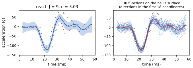
Figure 8.S5 (supplementary). Exercise 8. Left: react fit with \(J=9\) and its 95% band. Right: 30 functions on the surface of the 95% confidence ball (8.24), directions in the first 18 coordinates. Not a figure of the book. Code: fig_8_S5. Download: PDF · SVGExercise 8.9. Simulate \(n=1000\) observations of the Doppler model with \(\sigma=0.1\), 1 and 3; fit local linear regression and react, each with a 95 percent band, and compare.
Solution
One set of Normal errors, scaled by \(\sigma\); local linear with the tricube kernel and \(h\) by cross-validation over 50 values from 0.002 to 0.3; react with the nested modulator; bands with \(c\) from the tube formula. ISE is the average squared error on 600 grid points.
\(\sigma\) react: \(J\), ISE, \(c\) local linear: \(h\), ISE, \(c\) 0.1 249, 0.0032, 3.95 0.0056, 0.0021, 3.86 1 10, 0.035, 3.07 0.065, 0.029, 3.23 3 1, 0.084, 1.96 0.300, 0.080, 2.78 Both estimators lose the high-frequency oscillations as \(\sigma\) grows; at \(\sigma=3\) react keeps only the constant (and the band is a pointwise interval with \(c=1.96\), since \(\kappa_0=0\)), while local linear chooses the largest bandwidth searched. Local linear is somewhat better at every noise level here; its bandwidth adapts the effective number of parameters continuously, while react's nested fit must keep or drop whole frequencies. Both bands cover the smoothed curve, not \(r\): near 0 neither contains the true oscillations once \(\sigma\ge1\) (Figure 8.S6).
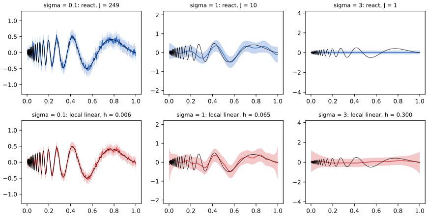
Figure 8.S6 (supplementary). Exercise 9: react (top) and local linear (bottom) fits with 95% bands, true function in black. Not a figure of the book. Code: fig_8_S6. Download: PDF · SVGExercise 8.10. Repeat Exercise 9 with Cauchy errors. How could the procedures be made more robust?
Solution
With \(0.1\times\)Cauchy errors (\(n=1000\)) both procedures collapse: a few huge observations dominate every \(Z_j\) and inflate \(\hs\) (the top coefficients are full of outliers), so react keeps \(J=1\) (ISE 0.092), and local linear cross-validation chooses the largest bandwidth (ISE 0.094). The \(Z_j\) have no variance, and SURE and the bands lose their meaning. A robust fix: replace the data by medians of consecutive blocks of \(m=5\) observations. The median of 5 Cauchy variables has finite variance and is close to Normal, and the 200 block medians form a regular design to which react applies unchanged: \(J=103\) and ISE 0.0094, ten times smaller (Figure 8.S7). Other options: Huber-type M-estimates of the coefficients, a robust scale (MAD of the top coefficients, as wavelet methods do in Chapter 9), or local median regression.
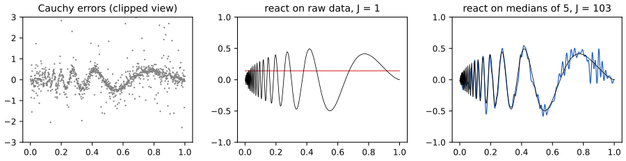
Figure 8.S7 (supplementary). Exercise 10: Cauchy errors. React on the raw data keeps only the constant; on medians of blocks of 5 it recovers the function. Not a figure of the book. Code: fig_8_S7. Download: PDF · SVGExercise 8.11. Draw \(n=1000\) points from \(\frac12\N(0,1)+\frac12\N(\mu,1)\), \(\mu=0,1,\dots,5\), and compare kernel density estimators with react density estimators.
Solution
React: rescale to \((a,b)\) = (min − 0.1·range, max + 0.1·range), nested modulator by (8.30), surgery. Kernel: Gaussian, \(h\) by least squares cross-validation, and the normal reference rule \(1.06\,s\,n^{-1/5}\). Integrated squared errors:
\(\mu\) react \(J\) react ISE LSCV \(h\) kernel ISE normal rule ISE 0 16 2.3e−3 0.27 7.2e−4 7.5e−4 1 5 6.7e−4 0.33 4.6e−4 4.7e−4 2 7 5.6e−4 0.39 5.0e−4 5.1e−4 3 9 4.6e−4 0.33 6.4e−4 9.6e−4 4 7 5.3e−4 0.33 6.7e−4 2.4e−3 5 11 4.6e−4 0.33 6.5e−4 4.2e−3 For a unimodal density (\(\mu\le2\)) the kernel estimates are better; react's choice is noisier (\(J=16\) for \(\mu=0\) is too many and adds wiggles at the top). For bimodal densities (\(\mu\ge3\)) react is slightly better than the cross-validated kernel estimate, and both are far better than the normal reference rule, which assumes one Normal and fills in the valley. These are single samples; the ranking of react and LSCV changes from sample to sample (try the demo's "new sample").
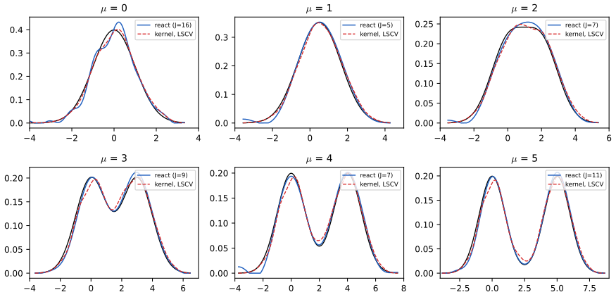
Figure 8.S8 (supplementary). Exercise 11: true density (black), react with surgery (blue) and the cross-validated kernel estimate (red, dashed). Not a figure of the book. Code: fig_8_S8. Download: PDF · SVGExercise 8.12. The greedy modulator \(b^*\) minimises \(R(b)\) over all modulators. (a) Find \(b^*\). (b) What goes wrong if \(b^*\) is estimated by minimising \(\Rh\) over all modulators?
Solution
(a) \(R(b)=\sum_j\{\th_j^2(1-b_j)^2+sb_j^2\}\) separates, and each term is a quadratic in \(b_j\) minimised at \(b_j^*=\th_j^2/(\th_j^2+s)\in[0,1]\), the Wiener filter, with risk \(\sum_j\th_j^2s/(\th_j^2+s)\), the smallest of all modulation estimators (the oracle).
(b) Minimising (8.15) term by term gives \(\hat b_j=(Z_j^2-\hat s)_+/((Z_j^2-\hat s)_++\hat s)\), with estimated risk \(\sum_j\hat s(Z_j^2-\hat s)_+/Z_j^2\). Each \(\hat b_j\) is chosen with its own noisy \(Z_j\): a coordinate whose noise happens to be large gets kept, one whose signal happens to be small gets dropped, and the estimated risk is evaluated at the coordinates that made it small. In 200 simulations of the Doppler model the greedy estimator's loss averaged \(5.1\times10^{-3}\), worse than the nested modulator's \(2.8\times10^{-3}\) and far above the oracle risk \(1.8\times10^{-3}\), while its estimated risk was only \(2.4\times10^{-3}\) (and \(-1.7\times10^{-3}\), negative, without the positive part): the estimate is badly optimistic (Figure 8.S9). The reason is the one in Filling the gap 8.5: over all modulators the weights \((1-b_j)^2\) are arbitrary, \(\sup_b|\Rt(b)-R(b)|\) is of order \(\sum_j|\xi_j|\approx n\cdot s=\sigma^2\), which does not vanish, whereas over monotone classes it is \(\OP(n^{-1/2})\).
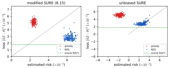
Figure 8.S9 (supplementary). Exercise 12: estimated risk against actual loss (units \(10^{-3}\)) for the greedy and nested modulators, with the modified (left) and unbiased (right) risk estimates; dashed: the oracle risk. Not a figure of the book. Code: fig_8_S9. Download: PDF · SVGExercise 8.13. Let \(Y_i=r(x_{1i},x_{2i})+\epsilon_i\), \(\epsilon_i\sim\N(0,1)\), \(r(x_1,x_2)=x_1+\cos(x_2)\), with \(x_{1i}=x_{2i}=i/n\). Generate 1000 observations, fit a tensor product model with \(J_1\) and \(J_2\) cosine functions, and choose \(J_1,J_2\) by SURE.
Solution
As stated, the two covariates coincide, so the data only see \(t\mapsto r(t,t)=t+\cos t\), and the tensor product design is singular (rank 5 for \(J_1=J_2=3\); Notes on the book). Taking \(x_1,x_2\) independent Uniform(0,1) instead: the design is irregular, so the fit is least squares on the \(J_1J_2\) products, and with \(\sigma=1\) known SURE is Mallows' \(C_p\), \(\mathrm{RSS}/n+2J_1J_2/n-1\). Over \(1\le J_1,J_2\le8\) it is smallest at \(J_1=J_2=2\), the four functions \(1,\phi_2(x_1),\phi_2(x_2),\phi_2(x_1)\phi_2(x_2)\) (Figure 8.S10). The fit captures the trend in \(x_1\) and the decrease in \(x_2\), but with one cosine per variable it bends a straight line flat at the ends (Filling the gap 8.2); with noise variance 1 and \(n=1000\), more terms do not pay. The true function is additive, and the selected interaction coefficient is small.
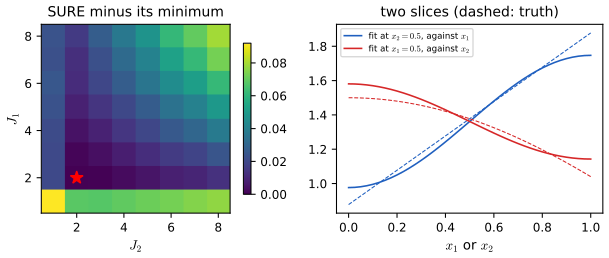
Figure 8.S10 (supplementary). Exercise 13 with independent uniform covariates: SURE over \((J_1,J_2)\) (left) and two slices of the selected fit against the truth (right). Not a figure of the book. Code: fig_8_S10. Download: PDF · SVGExercise 8.14. Air quality data: model ozone as a function of solar radiation, wind and temperature with a tensor product basis.
Solution
The data are R's airquality (New York, May to September 1973), 111 complete cases; each covariate is rescaled to \([0,1]\). Candidate models, all from the tensor cosine basis with \(J\) functions per variable: main effects only (additive), main effects and two-way interactions, and the full tensor product (\(J^3\) functions). Scores: leave-one-out cross-validation (exact shortcut for least squares).
model \(J\) functions \(R^2\) LOO CV constant 1 1 0 1117 additive 2 4 0.61 461 full tensor 2 8 0.69 388 additive 3 7 0.72 352 two-way 3 19 0.79 326 full tensor 3 27 0.80 375 additive 4 10 0.74 356 two-way 4 37 0.86 513 full tensor 4 64 0.92 1742 The two-way model with \(J=3\) (19 functions) predicts best; the full tensor product overfits quickly (64 functions for 111 observations), which is the curse of dimensionality of Filling the gap 8.13 in a small data set. The gain of the interactions over the additive fit is modest (326 against 352). Stronger smoothness on the interactions, as the book suggests, is what the two-way restriction does crudely.
Demonstrations for this chapter
| Demonstration | What you can see | Sections and results |
|---|---|---|
| React: orthogonal series regression | The coefficients, the noise estimate, the estimated risk of nested, monotone and constant modulators, the fit, the band (8.25) and the radius of the ball (8.24), on the Doppler, CMB, glass and motorcycle data. Presets: 1 Figure 8.1; 2 Figure 8.2, J = 6; 3 Figure 8.2, J = 40; 4 σ = 1 (Exercise 9); 5 motorcycle (Exercise 8). | 8.2, 8.3; Theorems 8.13, 8.17, 8.23 |
| The cosine basis: bias, smoothness and the boundary | The \(J\)-term approximation and the bias \(B_J\) on log-log axes for four functions; the equivalent kernel at any point. Presets: 1 periodic smooth; 2 a line, \(J^{-3}\); 3 a step; 4 Doppler; 5 the kernel at the boundary. | Lemma 8.4; Filling the gaps 8.2, 8.8, 8.12 |
| React density estimation | The series density estimate with its estimated risk curve and surgery, against kernel estimates, for mixtures of two Normals. Presets: 1 μ = 0; 2 μ = 2; 3 μ = 4; 4 μ = 5; 5 n = 200. | 8.4; Filling the gaps 8.10, 8.11; Exercise 11 |
Related demonstrations in the companion course Probability and Statistical Inference: cosine regression with a band and cosine density estimation. The Python code that produces every figure of this page is code/ch08_orthogonal_functions.py (see the code index).
References
- Wasserman, L. (2006). All of Nonparametric Statistics. Springer, New York. Chapter 8, pp. 183–195. www.stat.cmu.edu/~larry/all-of-nonpar.
- Beran, R. (2000). REACT scatterplot smoothers: superefficiency through basis economy. Journal of the American Statistical Association, 95, 155–171.
- Beran, R. and Dümbgen, L. (1998). Modulation of estimators and confidence sets. Annals of Statistics, 26, 1826–1856.
- Čencov, N. N. (1962). Evaluation of an unknown distribution density from observations. Soviet Mathematics, 3, 1559–1562.
- Efromovich, S. (1999). Nonparametric Curve Estimation: Methods, Theory and Applications. Springer, New York.
- Gao, F., Wahba, G., Klein, R. and Klein, B. (2001). Smoothing spline ANOVA for multivariate Bernoulli observations, with application to ophthalmology data. Journal of the American Statistical Association, 96, 127–160.
- Genovese, C. R., Miller, C. J., Nichol, R. C., Arjunwadkar, M. and Wasserman, L. (2004). Nonparametric inference for the cosmic microwave background. Statistical Science, 19, 308–321.
- Genovese, C. R. and Wasserman, L. (2005). Confidence sets for nonparametric wavelet regression. Annals of Statistics, 33, 698–729.
- Glad, I. K., Hjort, N. L. and Ushakov, N. G. (2003). Correction of density estimators that are not densities. Scandinavian Journal of Statistics, 30, 415–427.
- Härdle, W., Kerkyacharian, G., Picard, D. and Tsybakov, A. (1998). Wavelets, Approximation, and Statistical Applications. Springer, New York.
- Jang, W., Genovese, C. R. and Wasserman, L. (2004). Nonparametric confidence sets for densities. Technical report, Carnegie Mellon University.
- Lin, Y. (2000). Tensor product space ANOVA models. Annals of Statistics, 28, 734–755.
- Lin, X., Wahba, G., Xiang, D., Gao, F., Klein, R. and Klein, B. (2000). Smoothing spline ANOVA models for large data sets with Bernoulli observations and the randomized GACV. Annals of Statistics, 28, 1570–1600.
- Robertson, T., Wright, F. T. and Dykstra, R. L. (1988). Order Restricted Statistical Inference. Wiley, Chichester.
- Stein, C. M. (1981). Estimation of the mean of a multivariate normal distribution. Annals of Statistics, 9, 1135–1151.
- Wahba, G., Wang, Y., Gu, C., Klein, R. and Klein, B. (1995). Smoothing spline ANOVA for exponential families, with application to the Wisconsin Epidemiological Study of Diabetic Retinopathy. Annals of Statistics, 23, 1865–1895.
The numerical statements in the text (the discrete orthogonality of the cosines, the coefficient and bias rates, the consistency of the noise estimate, the risk identities, the PAV and clipping solutions, the variance of the pivot and the coverage of the ball, the band constants, the Gram–Schmidt basis, the density risk, the kernel identity, and the numbers of the examples and exercises) were confirmed numerically.