Chapter 10. Networks and Trees
Graphs record relations: which proteins interact, which states a Markov chain can move between, which species descend from which ancestor, which samples resemble each other. This chapter of Holmes and Huber (2019) uses graphs in three roles: as prior knowledge onto which experimental scores are projected (gene networks, Section 10.3), as parameters to be estimated from data (phylogenetic trees, Sections 10.4 and 10.5), and as summaries of data that support a nonparametric test (minimum spanning trees and the Friedman-Rafsky test, Section 10.6). The book is applied and states its probability models and test statistics without derivation; these notes give the derivations.
Ch. 1 Discrete data Ch. 2 Statistical modeling Ch. 3 Data visualization Ch. 4 Mixture models Ch. 5 Clustering Ch. 6 Testing Ch. 7 Multivariate analysis Ch. 8 Count data and GLMs Ch. 9 Heterogeneous data Ch. 10 Networks and trees Ch. 11 Image data Ch. 12 Supervised learning Ch. 13 Experimental design
How to read these notes
They follow the book. Sections carry the book's numbers (10.2, 10.4.3, ...) and titles, and figures carry the book's figure numbers, so the notes can be read next to the book. Questions that the book asks in the running text (Question 10.1 to 10.18) are answered where they arise.
Filling the gaps. Wherever the book states a model, a formula or a property without proof, an orange Filling the gap box gives the full argument, with its assumptions. Derivations start hidden: open one with its bar, or use the button below.
Figures and demonstrations. Every figure of the chapter computed from data or by simulation is reproduced by the course R code; numerical claims in these notes are verified numerically. The ▶ Demo boxes open an interactive demonstration already set to the case being discussed.
Main reference
S. Holmes and W. Huber, Modern Statistics for Modern Biology, Cambridge University Press (2019), Chapter 10, "Networks and Trees". Section, figure, question and exercise numbers below refer to this book. Further reading is listed in the references.
The explanations, derivations and code are my own; results are cited by their place in the book.
The chapter at a glance
- 10.2 A graph is a pair \((V,E)\), stored as an edge list or an adjacency matrix \(A\). Powers of \(A\) count walks, the Laplacian \(L=D-A\) is positive semidefinite and its kernel counts connected components, and a reduced Laplacian counts spanning trees (Gap 10.2). A Markov chain is a weighted directed graph; the chain of Figure 10.7 is absorbed in C after about 7 steps on average.
- 10.3 Enrichment of a category in a gene list is tested with the hypergeometric distribution (Fisher's exact test): 25 blue genes among 75 when 7.5 are expected has \(\Prob(X\ge25)=5.3\times10^{-9}\). Network methods fit a beta-uniform mixture to the p-values, turn each p-value into a log-likelihood-ratio score that is positive below an FDR threshold, and search for a connected subgraph of maximal total score (an NP-hard problem, solved heuristically).
- 10.4 Sequence evolution is a continuous-time Markov chain with \(\mathbf{P}(t)=e^{\mathbf{Q}t}\). For Jukes-Cantor, two sequences differ at a fraction \(p=\tfrac34(1-e^{-4d/3})\) of sites, so the Hamming proportion underestimates the distance \(d\) and \(\hat d\)
\({}=-\tfrac34\log(1-\tfrac43\hat p)\) is its maximum likelihood estimate. The likelihood of a tree is computed by Felsenstein's pruning recursion; neighbour joining is exact on tree distances. - 10.5 A phylogeny organises the hypotheses: test a clade first and its sub-clades only if it is rejected. Rejections are then closed under ancestors, and under the global null the probability of any rejection is at most the level.
- 10.6 The minimum spanning tree (MST) is found greedily (cut property). Colouring its vertices by a factor and counting pure edges gives the Friedman-Rafsky test, a multivariate runs test whose permutation null has an exact mean and variance (Result 10.6). With nested factors only the relabellings that respect the nesting are allowed: for litters of mice there are just 495 of them, so no p-value can be below 1/495.
Notation. \(G=(V,E)\) with \(n=|V|\) vertices; \(A\) adjacency matrix, \(D=\diag(d_1,\dots,d_n)\) degrees, \(L=D-A\) Laplacian. For substitution models: states \(\{A,C,G,T\}\), rate matrix \(\mathbf{Q}=(q_{ij})\), transition matrix \(\mathbf{P}(t)=(P_{ij}(t))\) with \(P_{ij}(t)\)
Prerequisites. Markov chains (Chapter 2), multiple testing and the false discovery rate (Chapter 6), mixture models (Chapter 4), distances and multidimensional scaling (Chapters 5 and 9), and the phyloseq containers for microbiome data.
Networks in biology carry meaning that must be stated: in a protein network (Figure 10.1) a node may be a gene or its protein and an edge a physical binding, a co-expression or a genetic interaction. The book uses "graph" for the mathematical object and "network" for its biological reading; so do these notes.
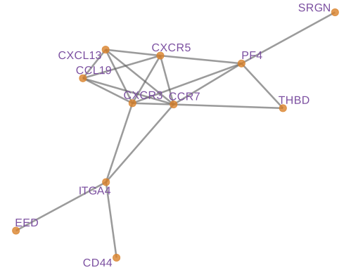
fig_10_1. Reproduces Holmes and Huber (2019), Figure 10.1. Download: PDF · SVG10.2 Graphs
10.2.1 What is a graph and how can it be encoded?
Definition 10.1 (graph, adjacency matrix, degree) Section 10.2.1
A graph \(G=(V,E)\) is a finite set \(V\) of vertices (nodes) with a set \(E\) of edges. In an undirected graph an edge is an unordered pair \(\{i,j\}\); in a directed graph it is an ordered pair \((i,j)\), an arrow from \(i\) to \(j\). A graph is simple if it has no loops \(\{i,i\}\) and no repeated edges. The edge list (from-to table) lists \(E\); the adjacency matrix is the \(n\times n\) matrix with \(A_{ij}=1\) if there is an edge from \(i\) to \(j\) and 0 otherwise (or the edge's weight, in a weighted graph). The degree of \(i\) in an undirected graph is \(d_i=\sum_j A_{ij}\), the number of edges at \(i\); in a directed graph the row sums are out-degrees and the column sums in-degrees.
The edge list and the adjacency matrix carry the same information, but not the same cost: the matrix needs \(n^2\) entries, the list \(|E|\) rows. A graph is sparse when \(|E|\) is of the order of \(n\) and dense when it is of the order of \(n^2\); the protein-interaction graph of the book (about 2,500 proteins and 20,000 edges) would waste more than 6 million zero entries in a full matrix, which is why sparse-matrix formats store only the non-zero entries. A drawing is not part of the graph: Figures 10.2 and 10.6 show the same graph as Figure 10.3, laid out differently.
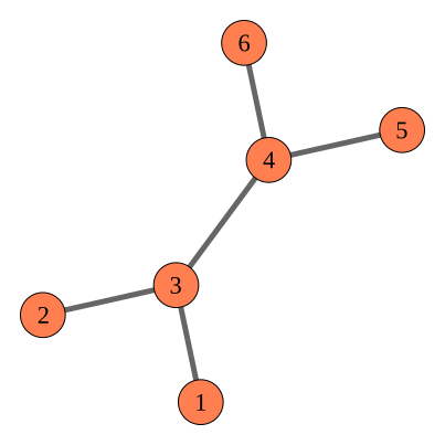
fig_10_2. Reproduces Holmes and Huber (2019), Figure 10.2. Download: PDF · SVG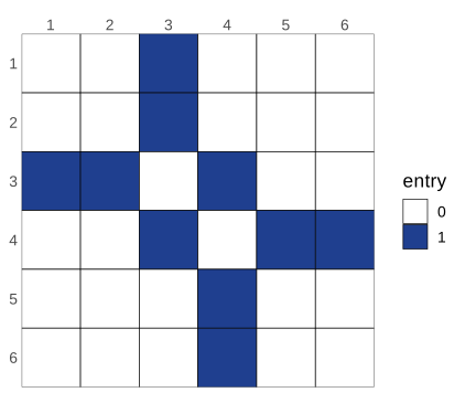
fig_10_3. Reproduces Holmes and Huber (2019), Figure 10.3. Download: PDF · SVGQuestion 10.1. For an undirected graph, \(\{i,j\}\in E\) if and only if \(\{j,i\}\in E\), so \(A_{ij}=A_{ji}\): the adjacency matrix is symmetric. (Question 10.2 asks for another way to build the graph from an edge list; reading a two-column table with graph_from_data_frame gives the same graph.)
Filling the gap 10.1: what the adjacency matrix counts Section 10.2.1, "Basic concepts"
Two facts make the adjacency matrix more than a storage format.
Derivation
Handshake lemma. In an undirected simple graph \(\sum_i d_i=2|E|\): the double sum \(\sum_i\sum_jA_{ij}\) visits every edge \(\{i,j\}\) twice, once as \((i,j)\) and once as \((j,i)\). So the average degree is \(2|E|/n\), and a sparse graph is one of bounded average degree.
Walks. A walk of length \(k\) from \(i\) to \(j\) is a sequence \(i=v_0,v_1,\dots,v_k=j\) with every consecutive pair an edge. Claim: \((A^k)_{ij}\) is the number of such walks. For \(k=1\) this is the definition. If it holds for \(k\), then
\[ (A^{k+1})_{ij}=\sum_{m}(A^k)_{im}A_{mj}, \]and the right side counts the walks of length \(k\) from \(i\) to some \(m\), each extended by the edge \(m\to j\) when it exists: every walk of length \(k+1\) arises exactly once this way, from its last step. Consequences: \(i\) and \(j\) are connected if and only if \((I+A)^{n-1}_{ij}>0\); \(\Tr(A^3)/6\) is the number of triangles of an undirected graph (each triangle gives 6 closed walks of length 3, from 3 starting points in 2 directions). We compare \(A^3\) with a brute-force count of walks on the graph of Figure 10.2. ∎
Definition 10.2 (paths, connectivity, cycles, trees) Sections 10.2.1 and 10.4
A path is a walk with distinct vertices; a graph is connected if every two vertices are joined by a path, and its maximal connected subgraphs are its components. A cycle is a closed walk of length at least 3 with distinct vertices apart from the end point. A tree is a connected graph without cycles; a leaf (tip) is a vertex of degree 1. A directed graph without directed cycles is a DAG (directed acyclic graph); the Gene Ontology is one.
Result 10.1 (characterisations of trees)
For a graph with \(n\) vertices the following are equivalent: (a) it is a tree; (b) it is connected and has \(n-1\) edges; (c) it has no cycle and has \(n-1\) edges; (d) every two vertices are joined by exactly one path. Every tree with \(n\ge2\) vertices has at least two leaves.
Proof
Leaves. Take a longest path in a tree; its end points have no neighbour outside the path (the path would extend) and no second neighbour on it (that would close a cycle), so both have degree 1.
(a) \(\Rightarrow\) (b). Induction on \(n\): remove a leaf and its edge; what remains is a tree on \(n-1\) vertices, which has \(n-2\) edges by hypothesis.
Counting components. Adding one edge to a graph either joins two components (and creates no cycle) or lies inside a component (and closes a cycle). Start from \(n\) isolated vertices and add the \(m\) edges one by one: if no cycle is ever closed, there are \(n-m\) components at the end. Hence an acyclic graph with \(n-1\) edges has one component, which is (c) \(\Rightarrow\) (a); and a connected graph with \(n-1\) edges must have merged components at every step, so it has no cycle, which is (b) \(\Rightarrow\) (a).
(a) \(\Leftrightarrow\) (d). Two different paths between the same vertices contain a cycle (follow them from the first point where they part to the first point where they meet again); conversely a cycle gives two paths between any two of its vertices. Connectivity is the existence of a path. ∎
Graph layout and the graph Laplacian
Drawing a graph means choosing a point \(y_i\in\R^2\) for every vertex. With edge lengths, this is the multidimensional scaling problem of Chapter 9. Without them, the Fruchterman-Reingold method lets edges pull their end points together and all vertices push each other apart, and stops at a balance of these forces. A cleaner relative of this idea is the spectral layout, which rests on the graph Laplacian.
Definition 10.3 (graph Laplacian)
For an undirected graph with (possibly weighted) symmetric adjacency matrix \(A\) and degree matrix \(D=\diag(d_1,\dots,d_n)\), \(d_i=\sum_jA_{ij}\), the Laplacian is \(L=D-A\).
Result 10.2 (properties of the Laplacian)
(a) For every \(x\in\R^n\),
\[ x^\T Lx=\sum_{\{i,j\}\in E}A_{ij}(x_i-x_j)^2 . \tag{10.2a} \](b) \(L\) is symmetric and positive semidefinite, and \(L\mathbf{1}=0\). (c) For nonnegative weights with \(A_{ij}>0\) exactly on the edges, the multiplicity of the eigenvalue 0 equals the number of connected components; in particular the second-smallest eigenvalue is positive if and only if the graph is connected. (d) Among layouts \(Y\in\R^{n\times2}\) with orthonormal, centred columns, \(\Tr(Y^\T LY)\)
Filling the gap 10.2: proofs for the Laplacian, and the matrix-tree theorem
The book draws graphs with layout algorithms and counts spanning trees implicitly when it discusses minimum spanning trees. The Laplacian connects both.
Derivation
(a) Expand: \(\sum_{i,j}A_{ij}(x_i-x_j)^2\)
(b) Symmetry is inherited from \(A\); positive semidefiniteness follows from (a) because every term is \(\ge0\); and \((L\mathbf{1})_i=d_i-\sum_jA_{ij}=0\).
(c) Since \(L\succeq0\), \(Lx=0\) if and only if \(x^\T Lx=0\), that is, \(x_i=x_j\) for every edge. Following paths, \(x\) is then constant on each component, and conversely every vector constant on each component is in the kernel. The indicator vectors of the \(c\) components are a basis of this space, so the kernel has dimension \(c\).
(d) \(\Tr(Y^\T LY)\)
Matrix-tree theorem (Kirchhoff). Let \(\tau(G)\) be the number of spanning trees of a connected simple graph (subgraphs that are trees and contain all vertices). Then, for any vertex \(i\), \(\tau(G)=\det L^{(i)}\), where \(L^{(i)}\) deletes row and column \(i\) of \(L\) (with \(A\in\{0,1\}\)). Proof: orient each edge arbitrarily and let \(B\) be the \(n\times|E|\) incidence matrix, with \(+1\) at the head and \(-1\) at the tail of each edge. Then \((BB^\T)_{ii}=d_i\) and \((BB^\T)_{ij}=-A_{ij}\), so \(L=BB^\T\) and \(L^{(i)}=B_iB_i^\T\), where \(B_i\) deletes row \(i\). By the Cauchy-Binet formula,
\[ \det L^{(i)}=\sum_{S\subset E,\ |S|=n-1}\det\big(B_i[\,\cdot\,,S]\big)^2 . \]If the \(n-1\) edges of \(S\) do not form a spanning tree they contain a cycle (Result 10.1), and the signed sum of the columns around the cycle is zero, so the determinant vanishes. If they form a spanning tree, the tree has a leaf \(v\ne i\) (it has at least two leaves); row \(v\) of \(B_i[\cdot,S]\) has a single non-zero entry \(\pm1\), and expanding along it leaves the matrix of the tree with \(v\) removed. By induction the determinant is \(\pm1\). So every spanning tree contributes exactly 1. For the complete graph \(K_n\) this gives Cayley's formula \(n^{n-2}\) (125 for \(n=5\), checked numerically, as is a small graph whose 21 spanning trees are enumerated by brute force). ∎
Graphs from data
Data rarely arrive as graphs. Two common constructions are used in this chapter. Thresholding a dissimilarity joins \(i\) and \(j\) when \(d(i,j)\le\delta\) (Figure 10.27). A bipartite graph has two kinds of vertices and edges only between kinds, and is stored as a rectangular 0/1 matrix: finch species by Galapagos islands (Figure 10.5), or transcription factors by the regions they bind.
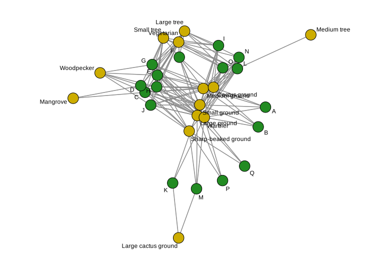
fig_10_5. Reproduces Holmes and Huber (2019), Figure 10.5. Download: PDF · SVG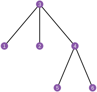
fig_10_6. Reproduces Holmes and Huber (2019), Figure 10.6. Download: PDF · SVGFigure 10.5 answers Question 10.3, Figure 10.6 Question 10.4. In the 13 by 17 incidence matrix the warbler finch occurs on all 17 islands and the medium tree finch on one.
An example: a four-state Markov chain
A Markov chain on a finite set of states is a weighted directed graph: the states are vertices and the transition probabilities \(P_{ij}>0\) are the weights of the arrows (Figure 10.7, the chain of Chapter 2 on the bases).
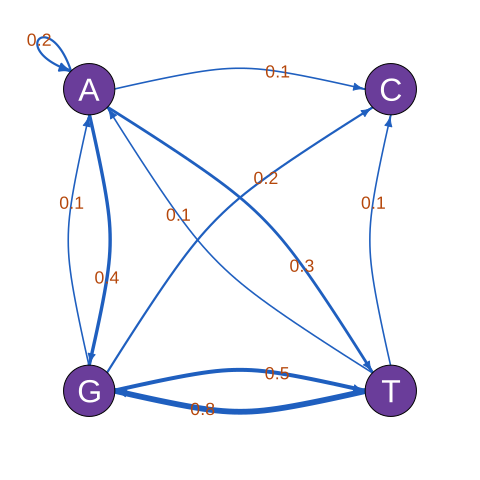
fig_10_7. Reproduces Holmes and Huber (2019), Figure 10.7. Download: PDF · SVGFilling the gap 10.3: where does the chain of Figure 10.7 end up? Question 10.5
The book's answer is that C is absorbing. Two further facts make this precise: absorption happens with probability one, and the expected time to absorption has a closed form.
\[ \mathbf{P}=\begin{pmatrix}0.2&0.1&0.4&0.3\\0&1&0&0\\0.1&0.2&0.2&0.5\\0.1&0.1&0.8&0\end{pmatrix}\quad(\text{rows and columns }A,C,G,T). \]Derivation
Order the states as transient \(\{A,G,T\}\) and absorbing \(C\), and let \(\mathbf{Q}_T\) be the \(3\times3\) block of transitions among the transient states. From every transient state the chain moves to C in one step with probability at least 0.1 (rows A: 0.1, G: 0.2, T: 0.1), so \(\Prob(\text{not absorbed after }k\text{ steps})\)
and 20,000 simulated runs from A take 6.98 steps on average. The chain spends most of its time in G before it is absorbed, because G and T send each other most of their mass. ∎
10.2.2 Graphs with many layers: labels on edges and nodes
Edges and vertices can carry attributes (type, weight, a score) that the drawing maps to colour, width and size. Figure 10.8 shows a chemokine subnetwork from the STRING database (Yu et al. 2012) with the gene names as labels; the group CXCR3, CXCL13, CCL19, CXCR5, CCR7 forms a near-clique. A graph stored with its attributes is the starting point of the subnetwork searches of Section 10.3.
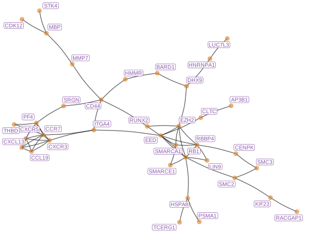
fig_10_8. Reproduces Holmes and Huber (2019), Figure 10.8. Download: PDF · SVG10.3 From gene set enrichment to networks
A differential-expression analysis (Chapter 8) produces a list of significant genes. Interpreting the list needs knowledge about the genes: which share a function, which interact. The section moves from sets of genes to networks of genes.
10.3.1 Methods using pre-defined gene sets (GSEA)
Gene sets come from curated sources: the three Gene Ontology vocabularies (a DAG whose edges point from a specific term to a more general one, so that a gene annotated with a term is implicitly annotated with all its ancestors), pathway databases and the Molecular Signatures Database. The statistical question is whether a set is over-represented among the significant genes.
10.3.2 Gene set analysis with two-way table tests
The book's toy example: a universe of \(N=1{,}000\) genes, of which 500 are yellow, 100 blue and 400 red; 75 genes are significant, 25 of each colour (Table 10.1). Equal counts do not mean equal enrichment, because blue genes are rare.
Definition 10.4 (hypergeometric distribution) Section 10.3.2
An urn holds \(N\) balls, \(K\) of them blue. Draw \(m\) without replacement, all \(\binom Nm\) subsets being equally likely. The number \(X\) of blue balls drawn has
\[ \Prob(X=x)=\frac{\binom Kx\binom{N-K}{m-x}}{\binom Nm},\qquad \max(0,m-N+K)\le x\le\min(m,K). \tag{10.3} \]Filling the gap 10.4: moments of the hypergeometric and Fisher's exact test Section 10.3.2, Question 10.6
The book simulates the null distribution (Figure 10.9) and states that the expected number of blue genes is "\(km/N\) ... in a draw of size \(k\)". With \(k\) the number of blue genes in the universe, the expected count is \(km/N\) in a draw of size \(m\) (the significant set), not of size \(k\).
\[ \E X=\frac{mK}{N},\qquad \Var X=m\,\frac KN\Big(1-\frac KN\Big)\frac{N-m}{N-1}. \tag{10.4} \]Derivation
(10.3): there are \(\binom Kx\) ways to choose the blue balls drawn and \(\binom{N-K}{m-x}\) to choose the others, among \(\binom Nm\) equally likely subsets.
Moments. Order the draw at random and let \(I_r=1\) if the \(r\)th ball is blue, so \(X=\sum_{r=1}^mI_r\). By symmetry each ball is equally likely to be any of the \(N\), so \(\E I_r=K/N\) and \(\E X=mK/N\). For \(r\ne s\), \(\Prob(I_r\)
Then \(\Var X\)
The exact p-value (Question 10.6). Observing 25 blue genes is 7 standard deviations above the mean. Its exact tail probability is
\[ \Prob(X\ge25)=\sum_{x=25}^{75}\frac{\binom{100}x\binom{900}{75-x}}{\binom{1000}{75}}=5.3\times10^{-9}, \]so a Monte Carlo experiment with 20,000 draws cannot see the event at all: the simulated p-value is \((0+1)/(20{,}000+1)\), an upper bound, not an estimate.
Fisher's exact test. Cross-classify the \(N\) genes by "blue or not" and "significant or not". If the significant set is a uniformly random subset of size \(m\) (the null hypothesis of no association, conditionally on both margins), the count in the cell "blue and significant" is hypergeometric (10.3). So the one-sided Fisher test of the table \(\begin{pmatrix}25&75\\50&850\end{pmatrix}\) has exactly the p-value above (fisher.test agrees to machine precision). Conditioning on the margins removes the nuisance parameters, which is why the test is "exact" in the sense of the book's margin note: its null distribution is known without approximation, not that its conclusion is certain. ∎
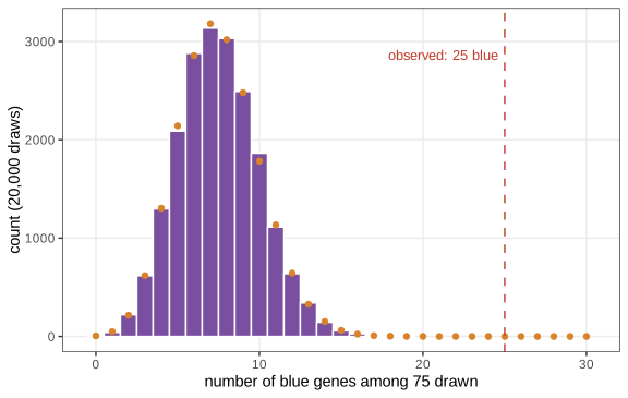
fig_10_9. Reproduces Holmes and Huber (2019), Figure 10.9. Download: PDF · SVGThe hypergeometric test treats genes as exchangeable draws, which they are not (co-regulated genes move together, and long genes are easier to call significant in RNA-seq); this is the main criticism of over-representation analysis and the motivation for methods that use the network.
10.3.3 Significant subgraphs and high scoring modules
Projecting gene-level scores onto a known interaction network (Ideker et al. 2002) asks for a connected set of genes whose scores are jointly high, a "perturbed module". Scores must be positive for interesting genes and negative for the others, otherwise the best subgraph is the whole network.
Definition 10.5 (maximum-weight connected subgraph)
Given a graph with a score \(s_v\in\R\) on each vertex, find a connected vertex set \(U\) maximising \(\sum_{v\in U}s_v\).
Filling the gap 10.5: why the subgraph search is "intractable" Section 10.3.3
The book says that finding the maximal scoring subgraph is NP-hard. A short reduction shows why.
Derivation
The Steiner tree problem in graphs (given a graph, a set \(T\) of terminal vertices and an integer \(k\), is there a connected subgraph containing \(T\) with at most \(k\) edges?) is NP-complete (Karp 1972). Build a vertex-weighted graph: subdivide every edge \(\{u,w\}\) by a new vertex \(e_{uw}\) of score \(-1\); give each terminal score \(M=|E|+1\) and every other original vertex score 0. A connected vertex set \(U\) of the new graph that contains all terminals corresponds to a connected subgraph of the original graph containing \(T\), and its score is \(|T|M\) minus the number of edge-vertices it uses. A set that misses a terminal scores at most \(|T|M-M<|T|M-|E|\). Hence the maximum score is at least \(|T|M-k\) if and only if a Steiner tree with at most \(k\) edges exists. A polynomial algorithm for the maximum-weight connected subgraph would therefore solve an NP-complete problem. In practice the Heinz algorithm of BioNet (Beisser et al. 2010) solves an integer programme or, in its fast version, runs a heuristic seeded by a minimum spanning tree of the positive-score components. ∎
10.3.4 An example with the BioNet implementation
The diffuse large B-cell lymphoma data of the DLBCL package give a t-test p-value for 3,583 genes (ABC against GCB subtype); restricted to the human interactome of the package, the network has 2,559 genes and 7,788 interactions after removing self-loops.
Definition 10.6 (beta-uniform mixture, BUM) Section 10.3.4
The p-values \(x_1,\dots,x_n\) are modelled as independent draws from
\[ f(x\given\lambda,a)=\lambda+(1-\lambda)\,a\,x^{a-1},\qquad 0<x\le1,\ 0<\lambda<1,\ 0<a<1, \tag{10.5} \]a mixture of the uniform density (true nulls) and the \(\mathrm{Beta}(a,1)\) density \(a x^{a-1}\) (signal), which is decreasing because \(a<1\) (Pounds and Morris 2003). Note that \(a x^{a-1}\) is itself a density (it integrates to 1), not just proportional to one.
Filling the gap 10.6: fitting the BUM model, the bound on \(\pi_0\), the FDR threshold and the node scores Section 10.3.4, Figures 10.10 and 10.11
The book fits the model with fitBumModel, scores the nodes "with an FDR of 0.001" and plots \(\pi_0\) without saying how each of these is defined. With \(F(x)=\lambda x+(1-\lambda)x^a\) the distribution function of (10.5):
Derivation
Maximum likelihood. The log-likelihood is \(\ell(\lambda,a)\)
with no closed-form solution, so \(\ell\) is maximised numerically over the open square. For fixed \(a\), \(\partial^2\ell/\partial\lambda^2\)
Why \(\lambda\) is not \(\pi_0\), and the upper bound. The beta component also puts mass near \(x=1\), so \(\lambda\) underestimates the proportion of true nulls. Suppose the p-value density is \(f=\pi_0\cdot1+(1-\pi_0)h\) with \(h\ge0\) the density of the non-null p-values. Then \(f(x)\ge\pi_0\) for every \(x\), so \(\pi_0\le\min_xf(x)=f(1)\) because \(f\) is decreasing. Hence \(\hat\pi_0\)
The threshold. Rejecting all p-values below \(\tau\) gives the estimated false discovery rate \(\widehat{\mathrm{FDR}}(\tau)\)
The scores. BioNet scores a gene by the log ratio of the signal density at its p-value to the signal density at the threshold:
\[ s(x)=\log\frac{(1-\lambda)a x^{a-1}}{(1-\lambda)a\tau^{a-1}}=(a-1)(\log x-\log\tau), \]positive exactly when \(x<\tau\) (because \(a-1<0\)) and negative otherwise. A gene with p-value \(10^{-10}\) scores \(0.82\times\log(1.93\times10^{6})\)
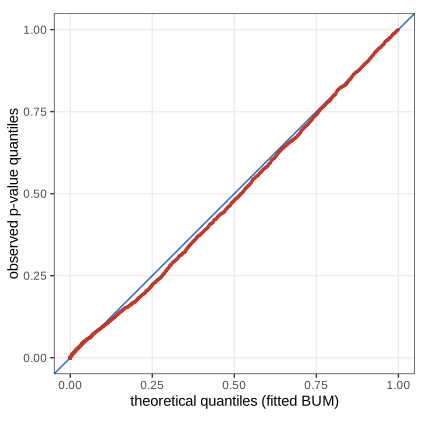
fig_10_10. Reproduces Holmes and Huber (2019), Figure 10.10. Download: PDF · SVG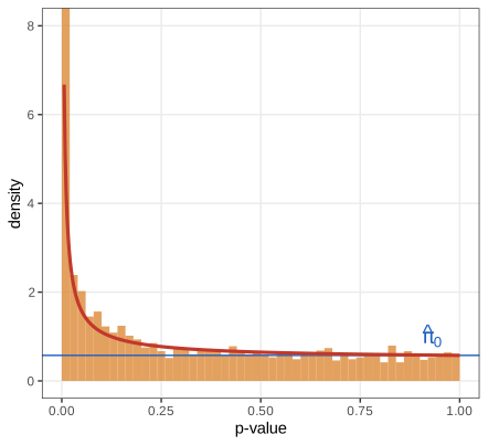
fig_10_11. Reproduces Holmes and Huber (2019), Figure 10.11. Download: PDF · SVGThe fast Heinz search on these scores returns a module of 144 genes and 221 interactions with total score 940.8 (the book, with an older package version, reports 149 genes and 234 interactions); 10 of its genes have negative scores and are included because they connect high-scoring regions. Question 10.7 asks to redraw the module with ggraph after converting it with igraph.from.graphNEL; Figure 10.12 is the package's own drawing.
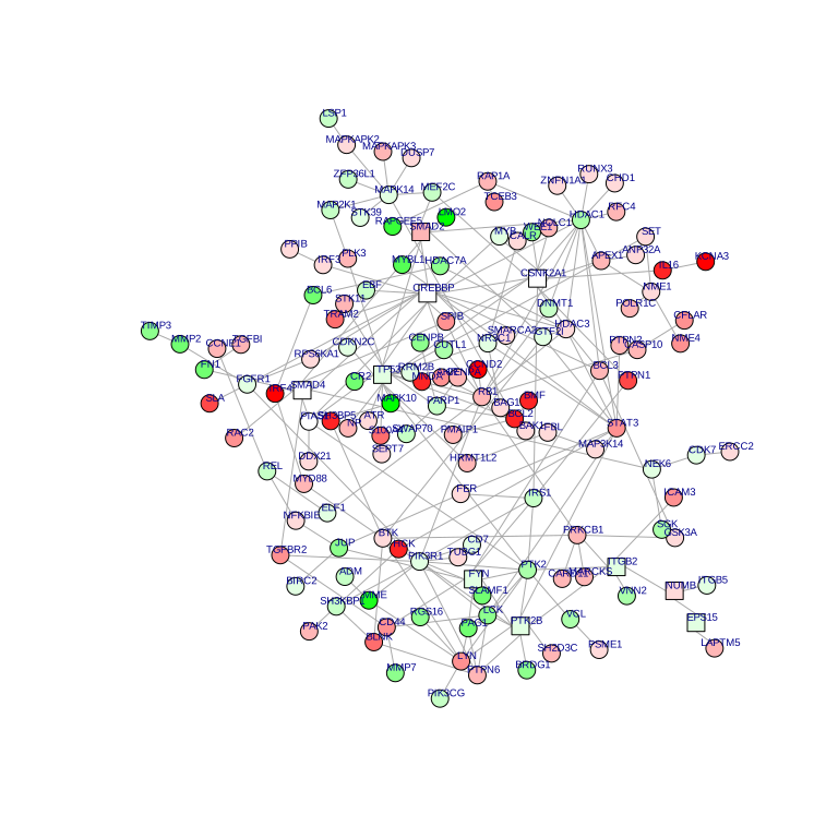
fig_10_12. Reproduces Holmes and Huber (2019), Figure 10.12. Download: PDF · SVG10.4 Phylogenetic trees
A phylogenetic tree is a tree (Definition 10.2) whose leaves carry the labels of present-day taxa (OTUs) and whose internal vertices stand for ancestors that are not observed. As mathematical objects, rooted binary trees with labelled tips are the same as the dendrograms of hierarchical clustering (Chapter 5); the difference is that here the tree is a parameter of a probability model for the sequences at the tips, together with its branch lengths and the substitution rates. Clades (monophyletic groups) are the sets of tips below an internal vertex; the root is usually placed by including an outgroup.
Definition 10.7 (phylogenetic tree, additive and ultrametric distances) Section 10.4
A phylogenetic tree on a label set \(X\) is a tree whose leaves are bijectively labelled by \(X\) and whose internal vertices have degree at least 3 (unrooted) or a root of degree 2 (rooted binary), with a length \(t_e>0\) on each edge. Its path metric \(d_T(i,j)\) is the sum of the edge lengths on the unique path between tips \(i\) and \(j\). A dissimilarity is additive if it is the path metric of some tree, and ultrametric if moreover all tips are at the same distance from a root (a molecular clock).
10.4.1 Markovian models for evolution
At one site of a sequence, the base along a lineage is a process \(Y(t)\in\{A,C,G,T\}\) that jumps at random times. The book lists the assumptions: the Markov property, time homogeneity and the linear form (10.1) of the short-time transition probabilities, with exponential times between changes,
\[ P_{ij}(h)=q_{ij}h+o(h)\ (j\ne i),\qquad P_{ii}(h)=1-q_ih+o(h),\quad q_i=\sum_{j\ne i}q_{ij}. \tag{10.1} \](The book prints \(1-q_i(h)\) for the second line; \(q_i\) is a rate, multiplied by \(h\).) A remark on the book's margin note: time homogeneity of \(\mathbf{Q}\) along a lineage is not the molecular clock. The clock is the further assumption that all lineages evolve at the same rate, which makes the tree ultrametric. Without it, rate and time enter each branch only through their product (the branch length), and only an unrooted tree with branch lengths is identifiable (Gap 10.14, the pulley principle).
Definition 10.8 (rate matrix; JC69, K80, F81, GTR) Section 10.4.1, Table 10.2
The rate matrix (generator) \(\mathbf{Q}\) has off-diagonal entries \(q_{ij}\ge0\) and diagonal \(q_{ii}=-q_i\), so every row sums to 0. In the state order A, C, G, T:
- Jukes-Cantor (JC69): \(q_{ij}=\alpha\) for all \(i\ne j\).
- Kimura two-parameter (K80): \(q_{ij}=\alpha\) for transitions (A\(\leftrightarrow\)G, C\(\leftrightarrow\)T, within purines or within pyrimidines) and \(\beta\) for transversions.
- Felsenstein (F81): \(q_{ij}=\mu\pi_j\), substitution towards base \(j\) in proportion to its frequency \(\pi_j\).
- General time-reversible (GTR): \(q_{ij}=s_{ij}\pi_j\) with \(s_{ij}=s_{ji}>0\) (exchangeabilities) and base frequencies \(\pi\).
Time is usually scaled so that the expected number of substitutions per unit time at stationarity, \(\sum_i\pi_iq_i\), equals 1; then a branch length \(d\) is the expected number of substitutions per site along the branch.
Result 10.3 (the transition matrix of a continuous-time chain)
Under the assumptions of (10.1) on a finite state space, \(\mathbf{P}(t)\) satisfies the Kolmogorov equations \(\mathbf{P}'(t)\)
The holding time in state \(i\) is exponential with rate \(q_i\), and when the chain leaves \(i\) it jumps to \(j\) with probability \(q_{ij}/q_i\).
Filling the gap 10.7: from (10.1) to \(e^{\mathbf{Q}t}\) and exponential waiting times
The book lists the properties of a continuous-time chain and moves on to the rate matrices. The link between them is (10.7).
Derivation
Chapman-Kolmogorov. By the Markov property and homogeneity, conditioning on the state at time \(t\), \(P_{ij}(t+h)\)
by (10.1) (the state space is finite, so the \(o(h)\) terms are uniform and the limit can be taken entrywise). Writing \(\mathbf{P}(t+h)\)
Holding times. Let \(g(t)=\Prob(\text{no jump in }[0,t]\given Y(0)=i)\). By the Markov property \(g(t+h)=g(t)\,(1-q_ih+o(h))\), so \(g'=-q_ig\) and \(g(t)=e^{-q_it}\): the waiting time is exponential with rate \(q_i\), as the book states. Given a jump in \([t,t+h]\), it goes to \(j\) with probability \(q_{ij}h/(q_ih)+o(1)\to q_{ij}/q_i\). Conversely, a chain built from exponential holding times and this jump rule satisfies (10.1). We confirm \(\mathbf{P}(s)\mathbf{P}(t)\)
Filling the gap 10.8: Jukes-Cantor transition probabilities
\[ P_{ii}(t)=\tfrac14+\tfrac34e^{-4\alpha t},\qquad P_{ij}(t)=\tfrac14-\tfrac14e^{-4\alpha t}\ (i\ne j),\qquad d=3\alpha t . \tag{10.8} \]Derivation
With \(J\) the \(4\times4\) matrix of ones, \(\mathbf{Q}=\alpha(J-4I)\). Since \(I\) commutes with \(J\), \(e^{\mathbf{Q}t}\)
Filling the gap 10.9: Kimura's model and its distance Question 10.8
K80 is more flexible than JC69 because it has two rates, and JC69 is the special case \(\alpha=\beta\) (Question 10.8). Starting from A, with \(d=(\alpha+2\beta)t\):
\[ P_{AG}(t)=\tfrac14+\tfrac14e^{-4\beta t}-\tfrac12e^{-2(\alpha+\beta)t},\qquad P_{AC}(t)=P_{AT}(t)=\tfrac14-\tfrac14e^{-4\beta t}, \tag{10.9} \]and if two sequences differ by a transition at a fraction \(P\) and by a transversion at a fraction \(Q\) of sites,
\[ \hat d_{\mathrm{K80}}=-\tfrac12\log(1-2P-Q)-\tfrac14\log(1-2Q). \tag{10.10} \]Derivation
Order the states A, G, C, T (purines first). \(\mathbf{Q}\) is symmetric with eigenvectors \(\mathbf{1}\) (eigenvalue 0), \((1,1,-1,-1)\) (purine against pyrimidine, eigenvalue \(-4\beta\): a transversion is needed to change the class) and \((1,-1,0,0)\), \((0,0,1,-1)\) (within the class, eigenvalue \(-2\alpha-2\beta\)). Each is checked by multiplying: e.g. the A row of \(\mathbf{Q}\) times \((1,1,-1,-1)\) is \(-(\alpha+2\beta)+\alpha-2\beta\)
the expected number of substitutions on the path. Substituting the observed proportions gives (10.10), the moment (and maximum likelihood) estimator. ∎
Filling the gap 10.10: reversibility of GTR and its number of parameters
The book calls GTR "the most flexible" model with 6 free parameters. It has 6 exchangeabilities \(s_{ij}\) and 4 base frequencies; one exchangeability is confounded with the time scale (only \(s_{ij}t\) enters \(\mathbf{P}\)) and the frequencies sum to 1, so a GTR model has 8 free parameters beyond the branch lengths (5 relative rates and 3 frequencies). Its key property is reversibility.
Derivation
Detailed balance. \(\pi_iq_{ij}\)
Real spectrum. With \(\Pi=\diag(\pi)\), the matrix \(\Pi^{1/2}\mathbf{Q}\Pi^{-1/2}\) has entries \(\pi_i^{1/2}s_{ij}\pi_j^{1/2}\) off the diagonal and is symmetric. So \(\mathbf{Q}\)
which is how phylogenetics software computes \(\mathbf{P}(t)\) for every branch from one eigen-decomposition. Detailed balance carries over: \(\pi_iP_{ij}(t)=\pi_jP_{ji}(t)\), because \(\Pi\mathbf{P}(t)\)
The rate in these models is the same for all sites. Real sequences have conserved and variable positions, which is modelled by rate heterogeneity (Gap 10.16).
10.4.2 Simulating data and plotting a tree
The book takes a 6-tip rooted tree, tree1 (Figure 10.15), as the true parameter and simulates 60 sites down it with simSeq(tree1, l = 60, bf = c(1,1,3,3)/8, rate = 0.1): a base is drawn at the root from the frequencies \(\pi=(\tfrac18,\tfrac18,\tfrac38,\tfrac38)\) for (a, c, g, t) and passed down each branch with the transition matrix for the branch length times 0.1 (Figure 10.16). Our seeded run gives 24 distinct site patterns and 25 variable sites (the book's unseeded run gave 27 patterns).
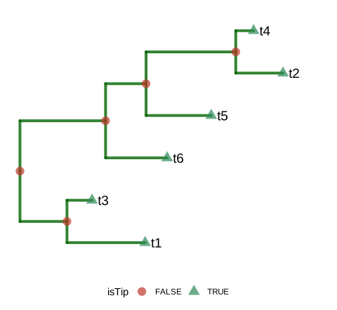
fig_10_15. Reproduces Holmes and Huber (2019), Figure 10.15. Download: PDF · SVG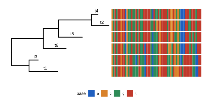
fig_10_16. Reproduces Holmes and Huber (2019), Figure 10.16. Download: PDF · SVGFilling the gap 10.11: what the simulation actually does (an F81 model, not Jukes-Cantor) Section 10.4.2, Figure 10.16
The caption of Figure 10.16 says that the sequences were generated "according to a Jukes Cantor model" with unequal frequencies at the root, and that mutations then occur down the tree. In simSeq, the argument bf is used twice: for the root and inside the rate matrix (\(q_{ij}\propto\pi_j\)). The model is F81, for which \(\pi\) is stationary, so the unequal frequencies are kept everywhere in the tree rather than washed out towards 1/4.
Derivation
Joint law of the tips. For a rooted tree with root \(\rho\), edges \(e=(u\to v)\) of length \(t_e\), and the states \(x\) at all vertices, the Markov property along the tree gives
\[ \Prob(x)=\pi^{(\rho)}_{x_\rho}\prod_{e=(u\to v)}P_{x_ux_v}(t_e), \]and the probability of the tip states sums this over the states of the internal vertices. The marginal law at a vertex \(v\) is \(\pi^{(\rho)}\mathbf{P}(t_{\rho v})\), with \(t_{\rho v}\) the length of the path from the root.
F81. With \(q_{ij}=\mu\pi_j\) (\(i\ne j\)), let \(\Pi_1=\mathbf{1}\pi\) (every row equal to \(\pi\)). Then \(\mathbf{Q}=\mu(\Pi_1-I)\), \(\Pi_1^2=\Pi_1\), and \(\mathbf{P}(t)\)simSeq builds.
JC69 with a non-uniform root. If the rate matrix were JC69 and only the root were unequal, the tip frequencies would be \(\pi^{(\rho)}\mathbf{P}(t)\)simSeq(..., bf = c(1,1,3,3)/8, rate = 1) gives tip frequencies 0.125, 0.125, 0.375, 0.375 to within 0.01, as F81 predicts. For the short branches of the book (rate 0.1) the two models would look alike, but the description is not what the code does. ∎
Question 10.9 (high mutation rates). Too few substitutions leave short internal branches without a trace; too many overwrite each other until the sequences are nearly independent (each pair differs at close to 3/4 of the sites), and the corrected distances become very noisy. So the probability of recovering the tree is low at both ends and peaks in between. In our simulation with 60 sites (phylogeny demo, preset 5) neighbour joining recovers the topology of tree1 in about 80% of data sets at rate 0.1, in about 20% at rate 0.01, and almost never above rate 3.
Filling the gap 10.12: why the Hamming distance underestimates, and the Jukes-Cantor correction Question 10.10
Let two sequences of \(L\) sites descend from a common ancestor under JC69, and let \(d\) be the expected number of substitutions per site on the path between them. Then the number \(K\) of differing sites is \(\Bin(L,p(d))\) with
\[ p(d)=\tfrac34\big(1-e^{-4d/3}\big),\qquad \dJC(\hat p)=-\tfrac34\log\Big(1-\tfrac43\hat p\Big),\qquad \Var\,\dJC(\hat p)\approx\frac{p(1-p)}{L\,(1-\tfrac43p)^2}, \tag{10.11} \]with \(\hat p=K/L\). The JC distance is the maximum likelihood estimate of \(d\), \(p(d)<d\) for every \(d>0\), and the relative bias \(1-p(d)/d\) grows with \(d\).
Derivation
The path between two tips. Let the ancestor be in stationarity and the two lineages evolve independently for times \(t_1,t_2\). Then \(\Prob(x_1\)
Maximum likelihood. \(d\mapsto p(d)\) is a strictly increasing bijection from \((0,\infty)\) onto \((0,\tfrac34)\). The binomial likelihood in \(p\) is maximised at \(\hat p=K/L\), so by invariance the likelihood in \(d\) is maximised at \(\hat d=p^{-1}(\hat p)=\dJC(\hat p)\) when \(\hat p<\tfrac34\); when \(\hat p\ge\tfrac34\) the likelihood increases without bound in \(d\) and the estimate is infinite ("saturation"). Maximising the binomial likelihood numerically recovers the formula.
Underestimation (Question 10.10, part 1). \(p(0)=0\), \(p'(d)=e^{-4d/3}\le1\) and \(p\) is strictly concave. Hence \(p(d)<d\) for \(d>0\): the observed proportion of differences counts at most one change per site and misses multiple hits and reversals.
The bias grows with \(d\) (part 2). \(p(d)/d\) is the slope of the chord from 0 to \(d\) of a concave function, which decreases in \(d\); so the relative bias \(1-p(d)/d\) increases. Taylor expansion gives \(p(d)=d-\tfrac23d^2+O(d^3)\), a relative bias of about \(\tfrac23d\): (exactly) 3.3% at \(d=0.05\), 27% at \(d=0.5\), 57% at \(d=1.5\). So the bias is smaller for small evolutionary distances, as the book's question suggests.
Standard error. By the delta method, \(\Var\hat d\)
10.4.3 Estimating a phylogenetic tree
The book lists four approaches: parsimony (the tree requiring the fewest changes, a Steiner tree problem, Figure 10.17), maximum likelihood under a substitution model, Bayesian posterior distributions over trees by MCMC, and distance methods (UPGMA and neighbour joining), which are "semi-parametric" because the distances come from a parametric model.
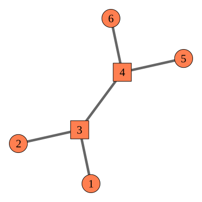
fig_10_17. Reproduces Holmes and Huber (2019), Figure 10.17. Download: PDF · SVGFilling the gap 10.13: computing the parsimony score of a tree, and the link with Steiner trees
For a fixed tree, the minimum number of substitutions needed to explain the tip sequences (the small parsimony problem) is computed by dynamic programming, one site at a time.
Derivation
Sankoff's recursion. For a site and a vertex \(v\), let \(c_v(s)\) be the minimum number of changes in the subtree below \(v\) given state \(s\) at \(v\). At a tip, \(c_v(s)=0\) for the observed base and \(+\infty\) otherwise. For an internal vertex with children \(w\),
\[ c_v(s)=\sum_{w}\min_{s'}\big(c_w(s')+\ind[s\ne s']\big). \]Correctness, by induction from the tips: once the state at \(v\) is fixed, the subtrees of the children share no edge, so the optimal total is the sum of the separately optimal costs, and for each child we choose its state \(s'\) and pay 1 on the edge \(v\to w\) if it differs. The score of the site is \(\min_sc_{\text{root}}(s)\); the tree's score sums over sites. Fitch's set algorithm is the same recursion written with sets of optimal states (for binary trees). The cost is \(O(n\cdot4^2)\) per site.
Steiner trees. Put the sequences in the space of all strings of length \(L\) with the Hamming metric. A labelled tree whose internal vertices are assigned sequences has total edge length equal to the number of changes, so the most parsimonious tree with its ancestral sequences is a minimum Steiner tree for the tip sequences, with the ancestors as Steiner points (Figure 10.17: vertices 3 and 4). For the book's simulated data our Sankoff score is 27 changes, both for tree1 and for the neighbour-joining tree, equal to phangorn::parsimony. Parsimony is fast and model-free, but it is not statistically consistent for all trees: with two long branches separated by a short one it converges to the wrong tree ("long-branch attraction", Felsenstein 1978). ∎
Result 10.4 (Felsenstein's pruning algorithm)
For a rooted tree with branch lengths, a reversible model with stationary distribution \(\pi\) and one site with tip states \(x\), define the partial likelihoods \(L_v(s)\)
The log-likelihood of an alignment is the sum over sites. The cost is \(O(nS^2)\) per site for \(S\) states, against \(O(nS^{n-1})\) for direct summation over the states of the \(n-1\) internal vertices.
Filling the gap 10.14: proof of the pruning algorithm, and why the root does not matter
The book says that maximum likelihood programs "use efficient optimization algorithms to maximize the likelihood of a tree" but not how the likelihood of one tree is computed. (10.12) is the answer.
Derivation
Recursion. Given \(X_v=s\), the processes in the subtrees of the different children are conditionally independent (each evolves from \(v\) by its own Markov transitions), so \(L_v(s)\) factorises over children. For one child \(w\),
\[ \Prob(\text{tips below }w\given X_v=s)=\sum_{s'}\Prob(X_w=s'\given X_v=s)\,\Prob(\text{tips below }w\given X_w=s',X_v=s)=\sum_{s'}P_{ss'}(t_w)L_w(s'), \]by the law of total probability and the Markov property (given \(X_w\), what happens below \(w\) does not depend on \(X_v\)). Finally \(\Prob(x)\)phangorn::pml (log-likelihood \(-213.83\) for tree1 with branch lengths times 0.1, \(-208.19\) for the NJ tree, both under JC69) and with a brute-force sum over all \(4^5\) internal states for one site.
Pulley principle (Felsenstein 1981). Suppose the root sits on the edge between \(a\) and \(b\), at distances \(t_1\) and \(t_2\). The root contributes the factor
\[ \sum_r\pi_rP_{ra}(t_1)P_{rb}(t_2)=\sum_r\pi_aP_{ar}(t_1)P_{rb}(t_2)=\pi_aP_{ab}(t_1+t_2), \]by detailed balance and Chapman-Kolmogorov. This depends on \(t_1+t_2\) only, so sliding the root along the edge, and then through vertex \(a\) onto any other edge, leaves the likelihood unchanged. Hence under a reversible model the likelihood is a function of the unrooted tree, and rate and time are not separately identifiable on a branch (only their product). Re-rooting tree1 at another tip leaves the log-likelihood unchanged to \(10^{-8}\).
Question 10.11. The book computes pml(tree1, seqs6, k = 4). With the true branch lengths at rate 1 (not the 0.1 used to simulate) the log-likelihood is \(-276.1\), far below the NJ tree's \(-210.5\), whose branch lengths are estimated from the data; with the lengths scaled by 0.1 the true tree is much closer. The comparison is fair only after optimising the branch lengths of both trees (optim.pml), which is how maximum likelihood compares topologies. A neighbour-joining branch can be negative (one here is \(-0.009\)); likelihood programs set it to zero. ∎
Algorithm 10.1 (neighbour joining; Saitou and Nei 1987, Studier and Keppler 1988)
- Start with the \(n\) taxa and their distance matrix \(d\).
- While more than three nodes remain (say \(m\)): compute \(R_i=\sum_kd_{ik}\) and \(Q_{ij}=(m-2)d_{ij}-R_i-R_j\) for \(i\ne j\); choose the pair \((i,j)\) with the smallest \(Q_{ij}\).
- Join \(i\) and \(j\) to a new node \(u\) with branch lengths \(d_{iu}\)
\({}=\tfrac12d_{ij}+\frac{R_i-R_j}{2(m-2)}\) and \(d_{ju}=d_{ij}-d_{iu}\). - Replace \(i,j\) by \(u\) with \(d_{uk}\)
\({}=\tfrac12(d_{ik}+d_{jk}-d_{ij})\) for every other node \(k\). - Join the last three nodes to a centre, with lengths from the three pairwise distances.
Filling the gap 10.15: where the neighbour-joining formulas come from, and when the method is exact
The book describes neighbour joining as similar to hierarchical clustering, with the joined pair summarised by a Steiner point. Three facts explain its formulas.
Derivation
Branch lengths. Suppose \(d\) is additive and \(i,j\) form a cherry with parent \(u\). For every other tip \(k\), the paths from \(i\) and \(j\) to \(k\) pass through \(u\), so \(d_{ik}-d_{jk}=d_{iu}-d_{ju}\). Averaging over the \(m-2\) other tips, \(d_{iu}-d_{ju}\)
The \(Q\) criterion is a tree-length criterion. Saitou and Nei estimate the total length \(S_{ij}\) of the tree in which \(i,j\) form a cherry and all other taxa hang from a single centre, by least-squares-type averages:
\[ S_{ij}=\frac{1}{2(m-2)}\sum_{k\ne i,j}(d_{ik}+d_{jk})+\frac{d_{ij}}2+\frac1{m-2}\sum_{\substack{k<l\\k,l\ne i,j}}d_{kl}. \]Let \(T=\sum_{k<l}d_{kl}\) be the sum over all pairs; then \(T=d_{ij}+\sum_{k\ne i,j}(d_{ik}\)
because \(R_i+R_j\)
Exactness. If \(d\) is the path metric of a tree with positive branch lengths, the pair minimising \(Q\) is a cherry of that tree (Saitou and Nei 1987; a full proof is given by Studier and Keppler 1988). Given this lemma, induction finishes the argument: joining a true cherry with the exact lengths and distances of steps 3 and 4 leaves the path metric of the tree with the cherry replaced by \(u\), so every step is correct. More generally, neighbour joining returns the correct topology whenever every entry of \(d\) is within half the shortest branch length of a tree metric (Atteson 1999). Numerically, NJ applied to the patristic distances of tree1 returns tree1 exactly (Robinson-Foulds distance 0, all path lengths equal), and my implementation agrees with ape::nj on the simulated data.
UPGMA (average-linkage clustering) is exact only for ultrametric distances, that is, under a molecular clock; neighbour joining does not need the clock. ∎
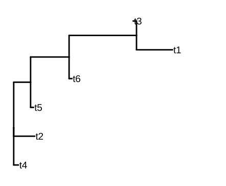
fig_10_18. Reproduces Holmes and Huber (2019), Figure 10.18. Download: PDF · SVGQuestion 10.12 (amino-acid sequences) uses \(20\times20\) rate matrices, usually empirical ones (such as WAG or JTT) with only the frequencies and branch lengths estimated; everything above carries over with \(S=20\) states. Uncertainty in the estimated tree is assessed with the bootstrap over sites or with Bayesian posterior samples of trees.
10.4.4 Application to 16S rRNA data
The 268 denoised sequence variants of Chapter 5 (seqtab.rds) are labelled by their own sequences and classified taxonomically with the naive Bayesian classifier of dada2 against the RDP training set (precomputed in taxtab16.rds; Question 10.13 prints its first rows). Taxonomy assigns names from a reference hierarchy; a phylogeny estimates the branching history and branch lengths from the sequences themselves, so two variants of the same genus can be far apart on the tree and an unnamed variant still has a place on it (Question 10.14). The variants are aligned with DECIPHER and a tree is fitted by maximum likelihood under GTR with rate heterogeneity, starting from the neighbour-joining tree.
Filling the gap 10.16: the GTR + \(\Gamma\) + I likelihood is a finite mixture
The book fits update(fit, k = 4, inv = 0.2) and then optimises with optGamma = TRUE, optInv = TRUE. These options make each site's rate random.
Derivation
Let a site be invariable with probability \(p_{\mathrm{inv}}\) (rate 0) and otherwise have rate \(r\) drawn from a gamma distribution with shape \(\kappa\) and mean 1, all branch lengths being multiplied by \(r\). By the law of total probability the site likelihood is
\[ \Prob(x)=p_{\mathrm{inv}}\,\Prob(x\given r=0)+(1-p_{\mathrm{inv}})\int_0^\infty\Prob(x\given r)\,g_\kappa(r)\,\d r, \]where \(\Prob(x\given r=0)=\pi_s\) if all tips show the same base \(s\) and 0 otherwise. Yang (1994) replaces the integral by an average over \(k\) equally probable categories, each represented by its conditional mean. With \(q_0=0<q_1\)
with \(G_{\kappa+1}\) the distribution function of shape \(\kappa+1\), rate \(\kappa\). For \(\kappa=1\), \(k=4\) this gives 0.137, 0.477, 1.000, 2.386, the values of phangorn::discrete.gamma (checked for three settings). Each site likelihood is then a mixture of \(k+1\) pruning computations (10.12). (phangorn rescales the non-zero rates by \(1/(1-p_{\mathrm{inv}})\) so that the average rate stays 1.) ∎
The fit takes about half an hour with stochastic rearrangements, so the course code caches it. Starting from the NJ tree under JC69 (log-likelihood \(-16{,}318.5\)), the GTR + \(\Gamma(4)\) + I tree reaches \(-12{,}769.8\), with gamma shape 0.507 and 29% invariable sites: a strongly heterogeneous rate across sites, as expected for a gene with conserved and variable regions. The fitted exchangeabilities are largest for the transitions C\(\leftrightarrow\)T (6.07) and A\(\leftrightarrow\)G (3.37) relative to G\(\leftrightarrow\)T (1).
10.5 Combining phylogenetic trees into a data analysis
A phyloseq object binds four tables that must stay consistent: the abundance table (samples by taxa), the sample data, the taxonomy and the tree. Subsetting one (for instance keeping samples with more than 5,000 reads, which leaves 10 of the 19 samples of pso) subsets the others. Question 10.15: the code computes the prevalence of each taxon (number of samples where it is present), tabulates the phyla, and keeps only the phyla represented by more than 5 taxa, a common filter against rare, unreliable taxa.
10.5.1 Hierarchical multiple testing
The question is which taxa change in abundance with age (three age bins) in the mouse data ps1 (344 samples, 389 taxa). Abundances are normalised with DESeq2 size factors and the variance-stabilising transformation of Chapter 8. Because most taxa are absent from some sample, the usual geometric mean of each taxon's counts is 0; the book therefore takes the geometric mean over the non-zero counts only, which makes the median-of-ratios size factors defined.
Algorithm 10.2 (hierarchical testing on a tree; Yekutieli 2008, as implemented in structSSI)
- For every vertex \(v\) of the tree, aggregate the transformed abundances of the tips below \(v\) and test the association with the covariate (structSSI's
treePValuesfits a one-way analysis of variance of the summed abundance on the age bin and uses its F-test p-value \(p_v\)). - Test the root at level \(\alpha\). If it is not rejected, stop.
- Whenever a vertex is rejected, apply the Benjamini-Hochberg procedure at level \(\alpha\) to the family formed by its children; recurse into every rejected child.
Filling the gap 10.17: what the hierarchical procedure guarantees Section 10.5.1
The book says the results "control several variants of FDR, but at different levels" and defers the details. Two properties are elementary, and the third is an estimate.
Derivation
(a) Rejections are closed upwards. A vertex is tested only if its parent was rejected, so every rejected vertex has a rejected parent, up to the root. The discoveries form a subtree containing the root, which is what makes them interpretable ("this genus, and within it these species"). We verify this on the result.
(b) Under the global null the procedure controls the family-wise error. If no taxon is associated, every aggregated test is null; any rejection requires the root to be rejected first, which has probability at most \(\alpha\) for a valid p-value. So \(\Prob(\text{any rejection})\le\alpha\), with no assumption on the dependence among the tests below the root.
(c) Within a family, BH controls the FDR at level \(\alpha\) times the proportion of nulls, under independence or positive dependence of that family's p-values (Chapter 6). Errors accumulate over the families that are tested, so the FDR over the whole tree is larger than \(\alpha\). Yekutieli (2008) bounds it by about \(\alpha\) times a factor that structSSI estimates as \((\#\text{discoveries}\)
Caveat. The F-tests treat the 344 samples as independent, although they come from 12 mice measured repeatedly, so the p-values are too small; a mixed model or a test that permutes whole mice (as in Section 10.6.3) would respect the design. ∎
What the package does today. In the current structSSI (version 1.2.1), hFDR.adjust tests the root and the family of its three children and then stops: its recursion looks for a column original_name that its own table does not have, so no deeper family is ever tested. The course code therefore implements Algorithm 10.2 directly (function hfdr_mine, which agrees with the package on the four hypotheses the package does test). With the book's \(\alpha=0.75\), 608 of the 776 hypotheses (389 tips and 387 internal vertices) are tested and 587 rejected, 284 of them tips. The p-values are extreme (the smallest adjusted tip p-value is \(4\times10^{-82}\)), a symptom of the caveat above: 344 samples from 12 mice are treated as independent. Figure 10.19 of the book is a screenshot of the interactive display and is not reproduced.
A correction to the book's table. The book joins the taxonomy to the test results by a column built from the row names of hfdr_res@p.vals; structSSI resets those row names to 1, 2, 3, ..., so the join matches nothing, the printed table shows NA for every hypothesis, and its rows are just the first taxa of the taxonomy table (Porphyromonadaceae, Bacteroidaceae, ...), which contradicts the text. Joining on the hypothesis names, the most significant tips are, in order, Lachnospiraceae (unclassified genus), Lachnospiraceae Roseburia, three Lachnospiraceae Clostridium XlVa and a Ruminococcaceae Ruminococcus; among the 284 rejected tips, 152 are Lachnospiraceae and 47 Ruminococcaceae. So the book's sentence "the most strongly associated bacteria all belong to family Lachnospiraceae" is right; its table is not.
10.6 Minimum spanning trees
Definition 10.9 (spanning tree, MST, Steiner tree) Section 10.6
A spanning tree of a connected graph is a subgraph that is a tree and contains every vertex. Given edge weights \(w_e\) (for points with a dissimilarity, the complete graph weighted by the dissimilarities), a minimum spanning tree (MST) minimises the total weight \(\sum_{e\in T}w_e\). A Steiner tree for a set of terminal points may add extra points (Steiner points) to shorten the total length.
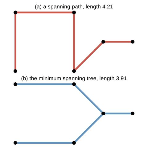
fig_10_20. Reproduces Holmes and Huber (2019), Figure 10.20. Download: PDF · SVGResult 10.5 (cut and cycle properties)
Let the edge weights be given. (a) Cut property: for any partition of the vertices into \(S\) and \(V\setminus S\), an edge of minimum weight among those crossing the cut belongs to some MST, and to every MST if it is the unique minimum. (b) Cycle property: an edge that is the unique heaviest edge of some cycle belongs to no MST. (c) If all weights are distinct, the MST is unique. (d) The MST depends on the weights only through their order: a strictly increasing transformation of all weights leaves the set of MSTs unchanged.
Algorithm 10.3 (Prim and Kruskal)
- Prim (1957): start from any vertex; repeatedly add the lightest edge joining the current tree to a vertex outside it, until all vertices are in. With a dissimilarity matrix this takes \(O(n^2)\) operations.
- Kruskal (1956): sort the edges by weight; go through them in order and keep an edge unless it closes a cycle with the edges kept so far.
Filling the gap 10.18: why the greedy algorithms find the MST, and the Steiner ratio Section 10.6
The book says that "greedy algorithms work well for computing the MST". They are in fact exact, because of the cut property.
Derivation
Cut property. Let \(e=\{u,v\}\) be a lightest edge crossing the cut and \(T\) an MST not containing \(e\). The path in \(T\) from \(u\) to \(v\) crosses the cut at some edge \(f\), with \(w_f\ge w_e\). Then \(T'=T-f+e\) is connected with \(n-1\) edges, so it is a spanning tree (Result 10.1), and \(w(T')\le w(T)\): \(T'\) is an MST containing \(e\). If \(e\) is the unique lightest crossing edge, \(w_f>w_e\) and \(T\) was not minimal, so every MST contains \(e\).
Cycle property. If the unique heaviest edge \(f\) of a cycle were in an MST \(T\), removing it splits \(T\) into two parts; the rest of the cycle crosses between them through a lighter edge \(e\), and \(T-f+e\) is lighter. Contradiction.
Uniqueness. With distinct weights, suppose \(T\ne T'\) are both MSTs and let \(e\) be the lightest edge in one but not the other, say \(e\in T\). Adding \(e\) to \(T'\) closes a cycle, which has an edge \(f\notin T\); \(w_f>w_e\) by the choice of \(e\) (distinct weights). Then \(T'-f+e\) is lighter than \(T'\). Contradiction.
Prim adds, at every step, a lightest edge across the cut (current tree, rest): by the cut property the tree built so far is always contained in some MST, so the final tree is one. Kruskal adds an edge \(e=\{u,v\}\) only when \(u,v\) are in different components of the kept forest; \(e\) is then a lightest edge across the cut (component of \(u\), rest), because every lighter edge has already been considered and either kept or found to lie inside a component. Again the forest stays inside some MST.
Order only. Kruskal's algorithm uses the weights only to sort them, so an increasing transformation produces the same tree (with ties broken the same way). This is why the MSTs for phyloseq's "Jaccard" and for Bray-Curtis coincide (Gap 10.21).
Ties. The 512 HIV sequences of Figure 10.21 have only 1,580 distinct distance values among 130,816 pairs, so their MST is far from unique, and different programs may draw different trees of the same total length. For the mouse data the MST is unique in the sense that matters: my Prim implementation and igraph::mst give the same edge set. With binary Jaccard distances, which have many ties, they do not (the number of pure edges differs by one).
Steiner trees. Adding Steiner points can only shorten the tree, but never by more than half: \(\text{MST}\le2\cdot\text{Steiner}\). Double every edge of an optimal Steiner tree; the result has a closed walk through every edge, of length \(2\cdot\text{Steiner}\), visiting all terminals. Skipping repeated and Steiner vertices (shortcuts, by the triangle inequality) gives a cycle through the terminals no longer than that, and deleting one of its edges gives a spanning tree of the terminals. For the four corners of a unit square the MST has length 3 and the Steiner tree \(1+\sqrt3\approx2.73\). Computing Steiner trees is NP-hard, MSTs are cheap, which is one reason the MST is so popular as a skeleton graph. ∎
The book's MST of HIV sequences from 2009 (Figures 10.21 to 10.23) uses DNA distances between 512 sequences of known country of origin, computed under the Jukes-Cantor model. Countries form branches of the tree (196 of its 511 edges join two sequences from the same country), and drawing the tree at the countries' coordinates shows the long-range links. Question 10.16 asks for repelling labels (Figure 10.22). Question 10.17 asks for a directed version: rooting the tree at one sequence and orienting every edge away from it gives a directed tree, but the direction is an assumption about the order of transmission, not something the distances reveal.
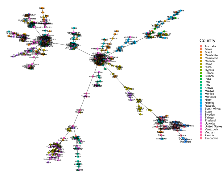
fig_10_21. Reproduces Holmes and Huber (2019), Figure 10.21. Download: PDF · SVG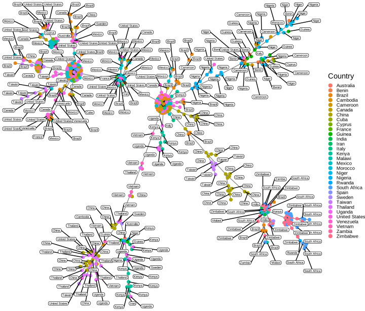
fig_10_22. Reproduces Holmes and Huber (2019), Figure 10.22. Download: PDF · SVG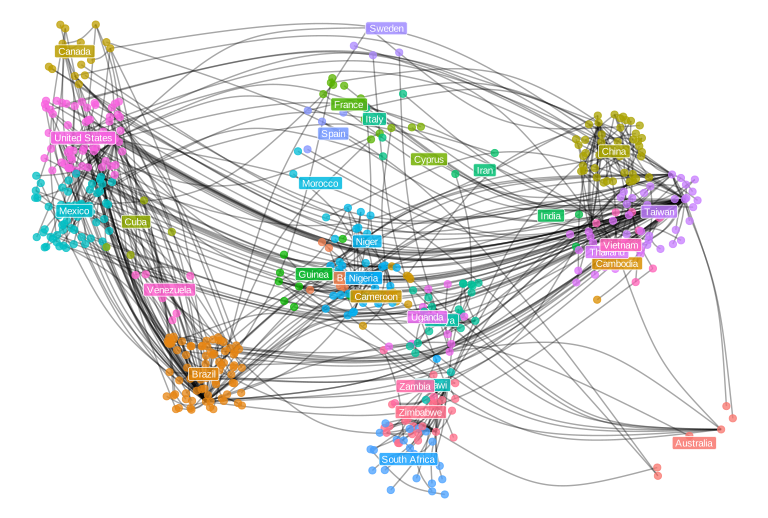
fig_10_23. Reproduces Holmes and Huber (2019), Figure 10.23. Download: PDF · SVG10.6.1 MST based testing: the Friedman-Rafsky test
A two-sample test asks whether two samples come from the same distribution. In one dimension the Wald-Wolfowitz test sorts the pooled sample and counts runs of the same label (Figure 10.24): few runs mean that the labels cluster along the line. Friedman and Rafsky (1979) noticed that sorting is the MST of points on a line, and replaced it by the MST in any space where a dissimilarity is defined.
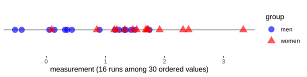
fig_10_24. Reproduces Holmes and Huber (2019), Figure 10.24. Download: PDF · SVGDefinition 10.10 (pure edges, the Friedman-Rafsky statistic) Section 10.6.1
Let a graph on \(N\) objects be built from their dissimilarities only (MST, k-nearest-neighbour graph, threshold graph), and give each object a label. An edge is pure if its two end points carry the same label and mixed otherwise. The test statistic is the number of pure edges \(S\) (equivalently the number of mixed edges, \(|E|-S\)); large \(S\) is evidence that objects with the same label are similar. The null distribution is that of \(S\) when the labels are randomly permuted.
Filling the gap 10.19: the null distribution of the number of runs Figure 10.24
Let \(m\) objects have label \(a\), \(n\) label \(b\), \(N=m+n\), and under the null hypothesis let all \(\binom Nm\) arrangements along the line be equally likely. The number of runs \(R\) has
\[ \E R=1+\frac{2mn}{N},\qquad \Var R=\frac{2mn(2mn-N)}{N^2(N-1)} . \tag{10.13} \]Derivation
Write \(R=1+\sum_{k=1}^{N-1}I_k\), with \(I_k=1\) when positions \(k\) and \(k+1\) carry different labels (a new run starts). For any two positions, \(\Prob(\text{labels }ab\text{ or }ba)\)
which simplifies to (10.13) (checked symbolically by enumerating all 462 arrangements of \(m=5\), \(n=6\)).
The link with the MST. For distinct points on a line, consider the gap between the \(k\)th and \((k+1)\)th smallest points. Every edge crossing the cut "left of the gap / right of the gap" spans the gap, and the edge between the two neighbouring points is the shortest of them. By the cut property it is in the MST, for every \(k\); these \(N-1\) edges are already a spanning tree. So the MST is the sorted path, its mixed edges are the run boundaries, and the number of mixed edges is \(R-1\). ∎
Result 10.6 (exact null mean and variance of the pure-edge count)
Let a graph with \(|E|\) edges be fixed, let \(C\) be the number of unordered pairs of edges that share a vertex, and let the \(N\) labels, with \(n_k\) of label \(k\), be randomly permuted. With \(a_k=n_k(n_k-1)\) and \(N_{(r)}=N(N-1)\cdots(N-r+1)\),
\[ f_2=\frac{\sum_ka_k}{N_{(2)}},\quad f_3=\frac{\sum_ka_k(n_k-2)}{N_{(3)}},\quad f_4=\frac{(\sum_ka_k)^2-\sum_ka_k(4n_k-6)}{N_{(4)}}, \] \[ \E S=|E|f_2,\qquad \Var S=|E|f_2+2Cf_3+2\Big[\tbinom{|E|}2-C\Big]f_4-(|E|f_2)^2. \tag{10.14} \]For two labels and the MST (\(|E|=N-1\)) the mean number of mixed edges is \(2mn/N\), the same as \(\E R-1\) in (10.13).
Filling the gap 10.20: proof of (10.14), and what it says about the mouse data Section 10.6.1
Derivation
Write \(S=\sum_{e\in E}J_e\) with \(J_e=1\) if edge \(e\) is pure. A random permutation of the labels makes every ordered tuple of distinct vertices equally likely to receive any ordered tuple of labels from the multiset. So \(\E J_e\)
Mice by mouse label. The MST of the 344 samples has 343 edges and \(C=535\) adjacent pairs; with 12 mice of 24 to 31 samples, \(\E S=27.85\) and \(\mathrm{sd}(S)=5.05\), and 20,000 permutations give 27.83 and 5.05. The observed 149 pure edges are 24 standard deviations above the mean. The Monte Carlo p-value \(1/1001\) printed by the book is simply the smallest value 1,000 permutations can give. ∎
10.6.2 Example: bacteria sharing between mice
The data ps1 hold 344 stool samples from 12 mice in two litters (4 mice and 114 samples in litter 1, 8 mice and 230 samples in litter 2), with counts of 389 sequence variants. The dissimilarity is phyloseq::distance(ps1, method = "jaccard").
Filling the gap 10.21: which "Jaccard" is used Section 10.6.2, Figure 10.33
The book says that it computes the Jaccard distance and recommends Jaccard for sparse co-occurrence data. In phyloseq, method = "jaccard" calls vegan::vegdist with its default binary = FALSE, which is the quantitative Jaccard index
computed from the abundances, not from presence and absence.
Derivation
It reduces to Jaccard on 0/1 data. For presence/absence vectors let \(a\) be the number of taxa present in both samples, \(b\) and \(c\) the numbers present in only one. Then \(\sum|x-y|=b+c\) and \(\sum(x+y)=2a+b+c\), so \(B=\frac{b+c}{2a+b+c}\) and \(\frac{2B}{1+B}\)
Same graphs as Bray-Curtis. \(B\mapsto2B/(1+B)\) is strictly increasing on \([0,1]\) (derivative \(2/(1+B)^2>0\)). Every construction that uses only the order of the dissimilarities (the MST, Result 10.5(d); the k-nearest-neighbour sets) is therefore identical for phyloseq's Jaccard and for Bray-Curtis. In particular Exercise 10.9, which uses Bray-Curtis, produces exactly the graph that the caption of Figure 10.33 attributes to the Jaccard similarity, so the caption is right about the graph even though the code uses another name. A threshold graph is not invariant in the same sense: \(J\le0.35\) is \(B\le0.35/1.65=0.212\). We confirm (10.15) to machine precision and the equality of the MSTs and 2-NN graphs. ∎
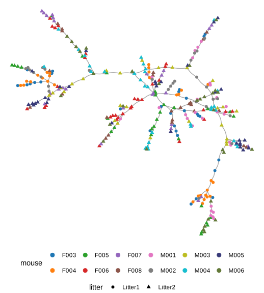
fig_10_25. Reproduces Holmes and Huber (2019), Figure 10.25. Download: PDF · SVG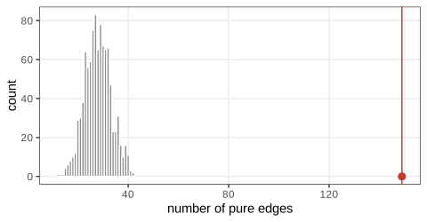
fig_10_26. Reproduces Holmes and Huber (2019), Figure 10.26. Download: PDF · SVGFilling the gap 10.22: why the permutation test is valid, and how small its p-value can be Sections 10.6.1 to 10.6.3
The book computes p-values as the proportion of permutations with at least as many pure edges, plus one. Two facts are needed: the graph must not depend on the labels, and the permutations must respect the structure of the null hypothesis.
Derivation
Exact permutation test. Let \(\mathcal G\) be a group of relabellings (all permutations of the samples, or only those allowed by the design) such that, under \(H_0\), the vector of labels \(\ell\) has the same distribution as \(g\ell\) for every \(g\in\mathcal G\), given the data used to build the graph. Since the graph is built from the abundances alone, \(S(g\ell)\) has the same distribution as \(S(\ell)\). Define \(p=\#\{g\in\mathcal G:S(g\ell)\ge S(\ell)\}/|\mathcal G|\). Conditionally on the orbit \(\{g\ell\}\), \(\ell\) is uniformly distributed over it, so \(p\) is the upper rank of a uniformly chosen element of a list, and \(\Prob(p\le\alpha)\le\alpha\) for every \(\alpha\).
Monte Carlo version. With \(B\) relabellings \(g_1\ell,\dots,g_B\ell\) drawn uniformly from \(\mathcal G\), the observed \(S(\ell)\) and the \(B\) simulated values are exchangeable under \(H_0\), so the rank of \(S(\ell)\) among the \(B+1\) values is (super-)uniform and \(\hat p\)
Restricted permutations (Section 10.6.3). Samples of the same mouse are alike whatever the litter, so permuting litter labels between samples would destroy the mouse structure and make litter look significant through the mouse effect alone (the demo shows this: free permutations put the observed 295 pure edges 12 standard deviations above the null mean). The null hypothesis "no litter effect beyond the mouse effect" makes the mice exchangeable between litters, so \(\mathcal G\) permutes litter labels among the 12 mice, keeping each mouse's samples together. With 4 mice in litter 1, \(\mathcal G\) produces only \(\binom{12}4=495\) distinct labellings. Hence:
- No p-value can be below \(1/495=0.00202\). For the MST, the observed labelling is the only one of the 495 with 295 or more pure edges, so the exact p-value is exactly \(1/495\); so is the exact p-value for the 1-NN graph (Figure 10.29) and for the 2-NN Bray-Curtis graph (Exercise 10.9).
- The Monte Carlo p-values of the book (0.004 for the MST with 1,000 draws, 0.002 for the k-NN tests with the default 499 draws) sample with replacement from these 495 labellings, so the observed one is drawn about \(B/495\) times and \(\hat p\approx(1+B/495)/(B+1)\): about 0.003 for \(B=1000\). Enumerating the 495 labellings is both faster and exact.
Different choices for the skeleton graph
Any graph built without the labels can replace the MST: the k-nearest-neighbour graph (an edge when either point is among the \(k\) nearest of the other, Schilling 1986) or a threshold graph. The 1-NN graph of the mouse samples has 272 edges: each of the 344 samples contributes one nearest-neighbour edge, and \(344-272=72\) pairs are mutual nearest neighbours, counted once. In general a k-NN graph has between \(Nk/2\) and \(Nk\) edges. The threshold graph at Jaccard dissimilarity 0.35 (Figure 10.27, built by make_network) keeps the 181 samples that have at least one neighbour that close, with 405 edges in 19 components.
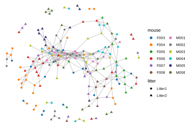
fig_10_27. Reproduces Holmes and Huber (2019), Figure 10.27. Download: PDF · SVG10.6.3 Friedman-Rafsky test with nested covariates
To test a litter effect beyond the differences between mice, the litter labels are permuted between mice (the grouping argument), as justified in Gap 10.22. The MST has 295 pure edges by litter, against a null mean of about 250 under the restricted permutations; the exact p-value is \(1/495\).
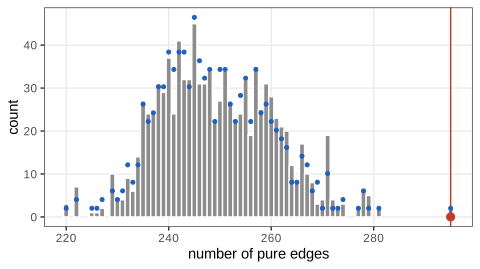
fig_10_28. Reproduces Holmes and Huber (2019), Figure 10.28. Download: PDF · SVGQuestion 10.18. With the 1-NN graph and nested permutations the test gives 236 pure edges among 272, again the most extreme of the 495 labellings (exact p-value 1/495; the book's Monte Carlo value is 0.002). Pairs of samples that are each other's nearest neighbours are much more often from the same litter than the mouse structure alone predicts, so the conclusion of the MST test does not depend on the choice of skeleton graph. The dual graph remark of the book applies the same machinery to taxa instead of samples (transpose the table) to study co-occurrence of bacteria.
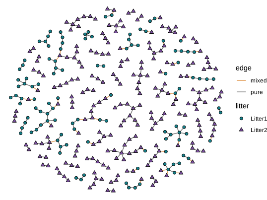
fig_10_29. Reproduces Holmes and Huber (2019), Figure 10.29. Download: PDF · SVGSummary
- Graphs are stored as edge lists or (sparse) adjacency matrices. Matrix powers count walks; the Laplacian \(L=D-A\) is positive semidefinite, its kernel counts components, its low eigenvectors give layouts, and its reduced determinants count spanning trees.
- Over-representation of a category is a hypergeometric (Fisher exact) test. Network methods convert p-values into scores through a beta-uniform mixture, with an FDR threshold that sets the sign of each score, and search for a high-scoring connected module, a problem that is NP-hard in general.
- Substitution models are continuous-time Markov chains with \(\mathbf{P}(t)=e^{\mathbf{Q}t}\). The Jukes-Cantor and Kimura corrections invert the saturation of the observed proportion of differences; the corrections are maximum likelihood estimates whose variance explodes near saturation.
- The likelihood of a tree is computed by Felsenstein's pruning recursion and, for reversible models, does not depend on the root. Parsimony is a Steiner tree problem in sequence space, solved for a fixed tree by dynamic programming. Neighbour joining is greedy minimum evolution and is exact on tree distances.
- A tree can organise hypotheses: testing children only after rejecting the parent gives discoveries that form a subtree and controls the error under the global null.
- The MST is computed greedily because of the cut property and depends on the dissimilarity only through its ranks. Counting pure edges of a skeleton graph gives the Friedman-Rafsky test, a multivariate runs test with an exact permutation mean and variance. Nested designs restrict the permutations, and then the number of distinct relabellings (here 495) bounds the attainable p-value.
Exercises
The exercises of Chapter 10 (Holmes and Huber 2019, Section 10.9), restated in my own words, with solutions (hidden).
Exercise 10.1. Write a function that draws a graph from its adjacency matrix, and show it on an example.
Solution
Reshape the matrix to long format (row, column, value) and draw one tile per entry, filled when the entry is 1, with the row axis reversed so the picture reads like the matrix. The course function
adjacency_tilesin ch10_networks_trees.R does this withgeom_tileandcoord_fixed; Figure 10.3 is its output for the graph of Figure 10.2. A node-link drawing is obtained instead withgraph_from_adjacency_matrixfollowed byplotorggraph.Exercise 10.2. For a gene list of your choice, extract from a Gene Ontology database the GO terms of the genes and build the graph of these terms and their ancestors.
Solution
Method: map the genes to GO identifiers with an organism annotation package (for example
org.Hs.eg.db, columnGO), restrict to one ontology, collect all ancestors of each term (GOBPANCESTORinGO.db), and add an edge from each term to each of its direct parents (GOBPPARENTS). The result is a DAG whose leaves are the most specific terms;igraphstores it as a directed graph andlayout_with_sugiyamadraws it in layers. No numerical answer is expected.Exercise 10.3. Represent the transitions between vaginal community state types (DiGiulio et al. 2015) as a Markov chain graph, with vertex size given by the fraction of preterm births and arrow width by the transition rate.
Solution
The data of this study are not distributed with the book (its code for Figure 10.30 is not live), so here is the statistical part. Given a sequence of observed states per woman, let \(n_{ij}\) count transitions from \(i\) to \(j\) and \(n_i=\sum_jn_{ij}\). The likelihood of a Markov chain is \(\prod_{i,j}P_{ij}^{n_{ij}}\) (given the first states); maximising \(\sum_jn_{ij}\log P_{ij}\) under \(\sum_jP_{ij}=1\) with a Lagrange multiplier gives \(n_{ij}/P_{ij}=\lambda_i\), so \(\hat P_{ij}=n_{ij}/n_i\), the observed transition proportions. These are the edge widths. The vertex sizes are the proportions of preterm births among women in each state; drawing them with
plot.igraphusesvertex.size,edge.widthandedge.curvedexactly as in Figure 10.7.Exercise 10.4. Use the STRING web site to save the edges around the gene CCNB1 (co-expression evidence only, confidence above 0.9, at most 50 interactors and nodes two steps away) as a text file.
Solution
Search CCNB1 for Homo sapiens, restrict the active evidence channels to co-expression, set the minimum confidence to 0.900, the first shell to at most 50 interactors and the second shell to 100, then export the "simple tab-delimited" text summary. The result used below is the file
ccnb1datsmall.txtdistributed with the book.Exercise 10.5. Read the file into R and draw the graph.
Solution
The file lists 207 edges between 43 proteins with their co-expression scores; CCNB1 has 17 direct neighbours. Build the symmetric weighted adjacency matrix by filling \(M_{ij}\) and adding the transpose (function
ccnb1in the course code; it is symmetric and every non-zero weight is at least 0.9), then draw it withgraph_from_adjacency_matrix(M, mode = "undirected", weighted = TRUE)andggraph, fixing the seed of the layout so the picture is reproducible.Exercise 10.6. Draw the adjacency matrix of Exercise 10.5 as a heatmap.
Solution
Figure 10.32:
heatmapreorders rows and columns by hierarchical clustering, the grey scale shows the co-expression weight (white below 0.9), and the side bars mark CCNB1 (blue) and its neighbours (red).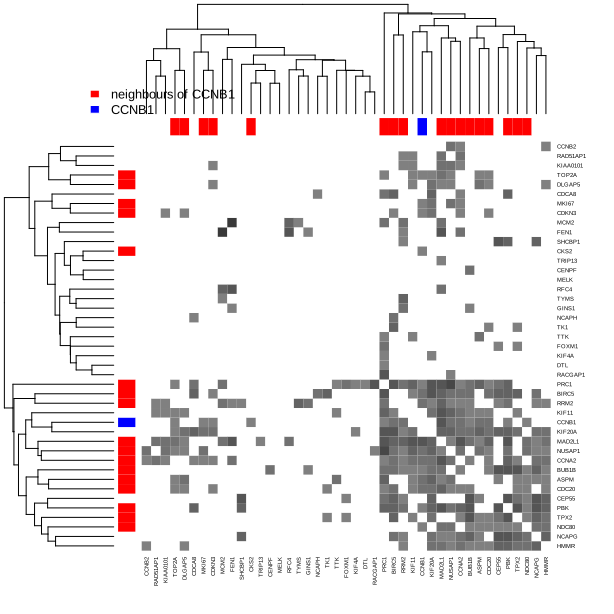
Figure 10.32. Heatmap of the CCNB1 co-expression adjacency matrix (43 proteins, weights 0.9 to 1 in grey, white below 0.9), rows and columns clustered; blue marks CCNB1, red its direct neighbours (Exercise 10.6). Code: ch10_networks_trees.R, fig_10_32. Reproduces Holmes and Huber (2019), Figure 10.32. Download: PDF · SVGExercise 10.7. The proteins co-expressed with CCNB1 are mostly co-expressed with each other, while proteins two steps away are not. Why, and which picture shows it better?
Solution
CCNB1 is a mitotic cyclin; its direct co-expression partners are other cell-cycle genes switched on together in G2/M, so they form a near-clique (high clustering). A protein two steps away is co-expressed with one of these partners for another reason (another process or another phase), and two such proteins need not share it: co-expression is not transitive. The heatmap shows this better, because clustering puts the clique in a dense block and the two-step proteins in sparse rows, whereas a node-link drawing of a dense block is a tangle whose density is hard to judge.
Exercise 10.8. For 20 HIV gag sequences, compute Jukes-Cantor distances with ape and with phangorn and compare them with the Hamming distances.
Solution
The alignment has 20 sequences of 1,746 sites with gaps. With
dist.dna(..., pairwise.deletion = TRUE)(ape), the mean proportion of differences over the 190 pairs is 0.1049, the mean JC69 distance 0.1144 and the mean K80 distance 0.1161; every JC distance exceeds its Hamming proportion and equals \(-\tfrac34\log(1-\tfrac43p)\) exactly.phangorn::dist.ml(..., "JC69")gives a mean of 0.1143, differing from ape by at most 0.0012: phangorn computes a maximum likelihood distance in which gaps and ambiguity codes contribute partial information instead of being deleted. The correction is small because the sequences are close (\(p\le0.16\)); by Gap 10.12 the relative difference is about \(2p/3\). The base composition is far from uniform (A 0.37, C 0.19, G 0.25, T 0.19), so a model with unequal frequencies (F81 or GTR) would fit better than JC69.▶ DemoHIV gag distancesThe 190 pairs, Hamming against JC69 and K80, computed in the browser and equal to ape's values.Exercise 10.9. Run the Friedman-Rafsky test for litter, with mice as groups, on the 2-nearest-neighbour graph of the Bray-Curtis dissimilarity.
Solution
The 2-NN graph has 516 edges, of which 430 are pure by litter (Figure 10.33). The package's Monte Carlo p-value with 499 draws is 0.002 (the book's value too); enumerating the 495 relabellings of the mice gives the exact p-value 1/495 = 0.00202, the smallest possible. By Gap 10.21 the graph is the same as for phyloseq's Jaccard dissimilarity.
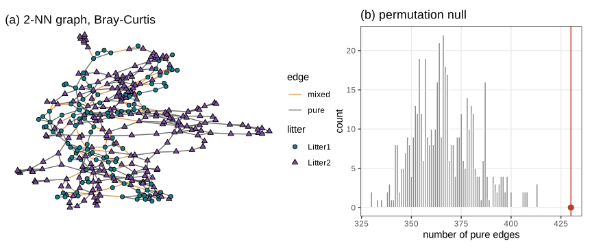
Figure 10.33. (a) The 2-nearest-neighbour graph of the Bray-Curtis dissimilarity (516 edges, 430 pure by litter) and (b) its nested permutation null; the observed count (red) exceeds every permuted value (Exercise 10.9). Code: ch10_networks_trees.R, fig_10_33. Reproduces Holmes and Huber (2019), Figure 10.33. Download: PDF · SVG
Demonstrations for this chapter
Each demonstration runs in the browser on the chapter's data, with seeded random numbers so that a class sees the same pictures, and links back to these notes. The ▶ Demo boxes above open them already set to the case under discussion.
| Demonstration | What you can see | Sections |
|---|---|---|
| Graph-based two-sample tests | MST, k-NN and threshold graphs on 344 mouse samples with three dissimilarities; pure and mixed edges; free and nested permutations, the exact null mean and variance, and the exact enumeration of the 495 litter relabellings; simulated two-sample data. Presets: 1 MST by mouse; 2 litter, nested; 3 1-NN; 4 2-NN Bray-Curtis; 5 free permutations for litter; 6 simulated null; 7 simulated shift. | 10.6 |
| Substitution models and evolutionary distances | JC69 and K80 transition probabilities, saturation of the Hamming proportion, the corrected distances on simulated pairs, and the HIV gag distances. Presets: 1 JC69; 2 short distance; 3 saturation; 4 K80; 5 HIV gag. | 10.4.1, Ex. 10.8 |
| Neighbour joining and the likelihood of a tree | Simulation down tree1, JC distances, neighbour joining step by step with its \(Q\) matrices, pruning log-likelihoods, and the probability of recovering the topology as a function of the mutation rate. Presets: 1 the book's data; 2 NJ steps; 3 too few mutations; 4 saturation; 5 the sweet spot; 6 more sites. | 10.4.2, 10.4.3 |
Each page reproduces the R values: the pure-edge counts (149, 295, 236 and 430), the null mean and standard deviation (27.85, 5.05), the exact p-values (1/495), the 190 gag distances, and the JC distances, NJ tree and log-likelihoods of the book's simulated data agree with the R code.
References
- Holmes, S. and Huber, W. (2019). Modern Statistics for Modern Biology. Cambridge University Press. Chapter 10.
- Atteson, K. (1999). The performance of neighbor-joining methods of phylogenetic reconstruction. Algorithmica, 25, 251–278.
- Beisser, D., Klau, G. W., Dandekar, T., Müller, T. and Dittrich, M. T. (2010). BioNet: an R-package for the functional analysis of biological networks. Bioinformatics, 26(8), 1129–1130.
- Benjamini, Y. and Hochberg, Y. (1995). Controlling the false discovery rate: a practical and powerful approach to multiple testing. Journal of the Royal Statistical Society: Series B, 57(1), 289–300. doi:10.1111/j.2517-6161.1995.tb02031.x.
- Felsenstein, J. (1978). Cases in which parsimony or compatibility methods will be positively misleading. Systematic Zoology, 27(4), 401–410.
- Felsenstein, J. (1981). Evolutionary trees from DNA sequences: a maximum likelihood approach. Journal of Molecular Evolution, 17, 368–376. doi:10.1007/BF01734359.
- Felsenstein, J. (2004). Inferring Phylogenies. Sinauer, Sunderland, MA.
- Fitch, W. M. (1971). Toward defining the course of evolution: minimum change for a specific tree topology. Systematic Zoology, 20(4), 406–416.
- Friedman, J. H. and Rafsky, L. C. (1979). Multivariate generalizations of the Wald-Wolfowitz and Smirnov two-sample tests. The Annals of Statistics, 7(4), 697–717. doi:10.1214/aos/1176344722.
- Henze, N. and Penrose, M. D. (1999). On the multivariate runs test. The Annals of Statistics, 27(1), 290–298.
- Ideker, T., Ozier, O., Schwikowski, B. and Siegel, A. F. (2002). Discovering regulatory and signalling circuits in molecular interaction networks. Bioinformatics, 18(Suppl. 1), S233–S240.
- Jukes, T. H. and Cantor, C. R. (1969). Evolution of protein molecules. In H. N. Munro (ed.), Mammalian Protein Metabolism, 21–132. Academic Press, New York.
- Karp, R. M. (1972). Reducibility among combinatorial problems. In R. E. Miller and J. W. Thatcher (eds.), Complexity of Computer Computations, 85–103. Plenum, New York.
- Kimura, M. (1980). A simple method for estimating evolutionary rates of base substitutions through comparative studies of nucleotide sequences. Journal of Molecular Evolution, 16, 111–120. doi:10.1007/BF01731581.
- Kruskal, J. B. (1956). On the shortest spanning subtree of a graph and the traveling salesman problem. Proceedings of the American Mathematical Society, 7(1), 48–50.
- McMurdie, P. J. and Holmes, S. (2013). phyloseq: an R package for reproducible interactive analysis and graphics of microbiome census data. PLoS ONE, 8(4), e61217.
- Pounds, S. and Morris, S. W. (2003). Estimating the occurrence of false positives and false negatives in microarray studies by approximating and partitioning the empirical distribution of p-values. Bioinformatics, 19(10), 1236–1242.
- Prim, R. C. (1957). Shortest connection networks and some generalizations. Bell System Technical Journal, 36(6), 1389–1401.
- Saitou, N. and Nei, M. (1987). The neighbor-joining method: a new method for reconstructing phylogenetic trees. Molecular Biology and Evolution, 4(4), 406–425. doi:10.1093/oxfordjournals.molbev.a040454.
- Sankaran, K. and Holmes, S. (2014). structSSI: simultaneous and selective inference for grouped or hierarchically structured data. Journal of Statistical Software, 59(13), 1–21.
- Sankoff, D. (1975). Minimal mutation trees of sequences. SIAM Journal on Applied Mathematics, 28(1), 35–42.
- Schilling, M. F. (1986). Multivariate two-sample tests based on nearest neighbors. Journal of the American Statistical Association, 81(395), 799–806.
- Studier, J. A. and Keppler, K. J. (1988). A note on the neighbor-joining algorithm of Saitou and Nei. Molecular Biology and Evolution, 5(6), 729–731.
- Tavaré, S. (1986). Some probabilistic and statistical problems in the analysis of DNA sequences. Lectures on Mathematics in the Life Sciences, 17, 57–86.
- Wald, A. and Wolfowitz, J. (1940). On a test whether two samples are from the same population. The Annals of Mathematical Statistics, 11(2), 147–162.
- Yang, Z. (1994). Maximum likelihood phylogenetic estimation from DNA sequences with variable rates over sites: approximate methods. Journal of Molecular Evolution, 39, 306–314.
- Yekutieli, D. (2008). Hierarchical false discovery rate-controlling methodology. Journal of the American Statistical Association, 103(481), 309–316.
The numbers quoted in the text (exact tail probabilities, absorption times, BUM estimates and thresholds, distances, log-likelihoods, null moments and exact p-values) come from the course R code; the figures come from ch10_networks_trees.R.