Reproducing the Book's Figures in Python
Every numerical experiment and figure of Chapters 1 to 14 of Bishop's Pattern Recognition and Machine Learning (2006), rebuilt from scratch with numpy, scipy and matplotlib: 193 figures from 15 modules, one function per figure, and readable implementations of every algorithm with docstrings that cite the book's equations.
How to run it
Download the files of this folder (common.py, make_all.py, the chapter modules and checks below, requirements.txt and data/faithful.csv), keeping the layout, then
pip install -r requirements.txt
python3 make_all.py                     # every figure, then every numerical check
python3 ch09_mixture_em.py --fig 9.1    # one figure
python3 ch12_continuous_latent.py --list
python3 checks_ch10a.py                 # the numerical checks for Sections 10.1-10.4
Each figure is written to ../img/chNN/figX-Y as a vector PDF (for slides and papers), a vector SVG (what the notes display, sharp at any zoom) and a PNG (thumbnails); change the folder with --out. Data: Old Faithful ships with the code (the same 272 eruptions as R's datasets::faithful); the oil flow data (Bishop and James 1993) and MNIST are downloaded once into ~/.cache/prml-repro; the photographs of Figure 9.3 are public-domain images bundled with matplotlib and scikit-image.
All the shared helpers (data loaders, plotting style, the command-line driver) are in common.py. Seeds are fixed, so every run gives the same pictures.
Chapter 1: Introduction
Source: ch01_introduction.py · run python3 ch01_introduction.py --list to list its figures · lecture notes: ch01-introduction.html
Module notes: data, settings and differences from the book
Bishop (2006), Chapter 1: Introduction.
Reproduces the numerical figures of Chapter 1 of C. M. Bishop, Pattern Recognition and Machine Learning (Springer, 2006), pp. 1-58, written from scratch with numpy, scipy and matplotlib. Every computation is a small function meant to be read next to the lecture notes (ch01-introduction.html):
* Section 1.1, polynomial curve fitting: design_matrix, fit_poly (the normal equations (1.122) solved stably by least squares, and the regularised error (1.4) by stacking sqrt(lambda) I under the design matrix), sse, rms_error (1.3). * Section 1.2.5-1.2.6, probabilistic and Bayesian curve fitting: map_poly (MAP = regularised least squares with lambda = alpha/beta, (1.67)), bayes_predictive (the predictive mean and variance (1.69)-(1.72), with S^{-1} = alpha I + beta sum phi phi^T). * Section 1.2.4, the Gaussian: gauss_pdf, gauss_ml (1.55)-(1.56), expected_ml_variance (1.58). * Section 1.4: shell_fraction (1.76 and Fig. 1.22), radial_density (Fig. 1.23). * Section 1.5, decision theory: bayes_decision (minimum expected loss (1.81)), expected_loss, reject_decision and decide_with_reject (Section 1.5.3, threshold theta, reject cost lambda = 1 - theta), error_probability (1.78 for two classes). * Section 1.6, information theory: entropy (1.93), kl_discrete (1.113), kl_gauss (closed form for two univariate Gaussians), discretised_gaussian_hist (Fig. 1.30). * js_noisy_sine: the data generator. It uses the seeded generator JSRandom (the generator DK.rng of the browser demos, imported from ch11_sampling.py), so curve-fitting-demo.html draws exactly the same data sets as the figures below.
Figures: 1.1-1.8, 1.11-1.17, 1.19-1.24, 1.26-1.31, plus "T1.1" (Table 1.1: the coefficients). Run `python3 ch01_introduction.py --list`, `python3 ch01_introduction.py` (all, about a minute) or `python3 ch01_introduction.py --fig 1.4 1.17`. Files go to ../img/ch01/.
Settings chosen where the book gives none (the book's data sets are not available): * Data (Figures 1.2-1.8, 1.16, 1.17, Table 1.1): t = sin(2 pi x) + Gaussian noise with standard deviation 0.3 (so beta = 1/0.3^2 = 11.1, as in the caption of Fig. 1.17), x_n = (n-1)/(N-1) equally spaced on [0, 1]. Training set N = 10 (DATA_SEED = 6, JSRandom); N = 15 and N = 100 sets of Fig. 1.6 use the same generator and seed; the test set of Figs 1.5 and 1.8 has 100 points (TEST_SEED), generated the same way. DATA_SEED is the first seed whose M = 9 fit over-fits as strongly as in the book (test RMS error of M = 9 above 0.8). * Figure 1.8 plots ln lambda from -35 to -5 (the book shows -35 to -20 and the book's test error is smallest near the right-hand end of that range; with our data it is smallest near ln lambda = -10, where E_RMS(test) = 0.37). * Fig 1.11: the 60 points are not recoverable, so we draw 60 points from the 9 x 2 table of counts read off the book's figure (COUNTS_1_11), with uniform jitter inside each cell. * Fig 1.15: three samples of size N = 2 from N(0, 1) (the book's are not given), plus a fourth panel (d) with the average of sigma^2_ML over 10^5 data sets against N (not in the book). * Fig 1.19-1.20: the three-phase oil flow data of Appendix A (1000 training points, x6 against x7), the test point x = (0.4, 1.3), 4 x 4 cells of width 0.25 and 0.5; 1.21 draws 4^D cells (D = 1, 2, 3). * Fig 1.23: Gaussian with sigma = 1/2 (the peak heights 1.60 for D = 1 and 1.2 for D = 2 in the book's axes imply it). * Fig 1.24: schematic in the book; we use p(x, C1) = 0.4 N(3, 1.3^2) + 0.2 N(7.2, 1^2) and p(x, C2) = 0.4 N(7.3, 1^2) on [0, 11] and x_hat = 7.3 (the peak of p(x, C2)); the shaded areas are computed. Fig 1.26 uses p(C2|x) = 0.72 s(6x) + 0.28 s(4(x - 3)) (a made-up posterior with a plateau). * Fig 1.27: p(x|C1) = 0.25 N(0.2, 0.075^2) + 0.75 N(0.5, 0.14^2), p(x|C2) = N(0.7, 0.1^2), equal priors: the book's mixture parameters are not given, so these resemble its curves (the book's p(x|C1) is not exactly normalised). * Fig 1.28: y(x) = sin(2 pi x) with Gaussian noise of standard deviation 0.3 around it. * Fig 1.30: discretised Gaussians over 30 bins with standard deviations (in bins) 1.42 and 5.49, which give H = 1.77 and H = 3.09 as in the book (the uniform distribution has ln 30 = 3.40). * Schematic figures not reproduced (they carry no numbers): 1.9, 1.10, 1.18 (cross-validation).
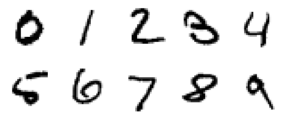
fig1_1() · in the notes · PDF · SVG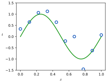
fig1_2() · in the notes · PDF · SVG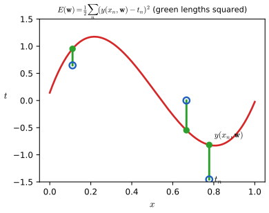
fig1_3() · in the notes · PDF · SVG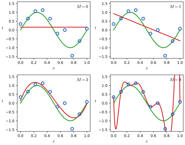
fig1_4() · in the notes · PDF · SVG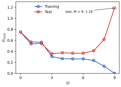
fig1_5() · in the notes · PDF · SVG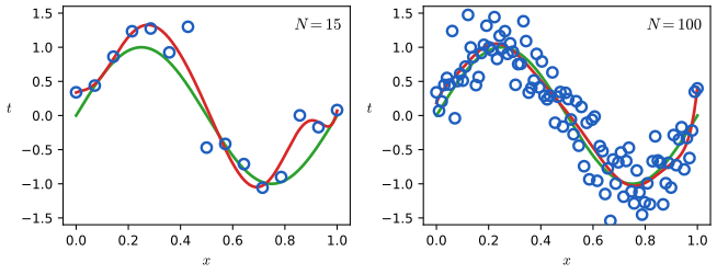
fig1_6() · in the notes · PDF · SVG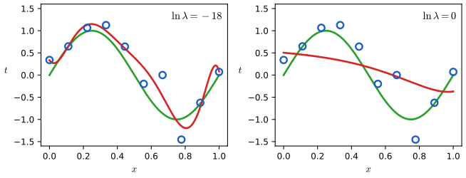
fig1_7() · in the notes · PDF · SVG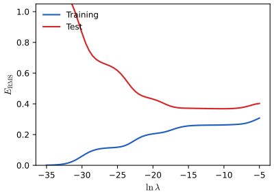
fig1_8() · in the notes · PDF · SVG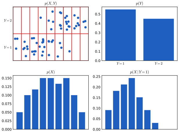
fig1_11() · in the notes · PDF · SVG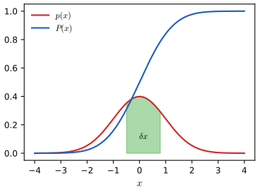
fig1_12() · in the notes · PDF · SVG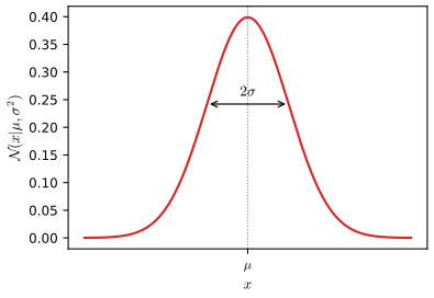
fig1_13() · in the notes · PDF · SVG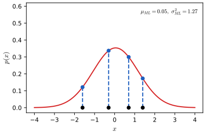
fig1_14() · in the notes · PDF · SVG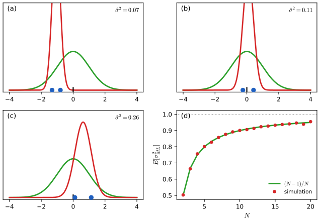
fig1_15() · in the notes · PDF · SVG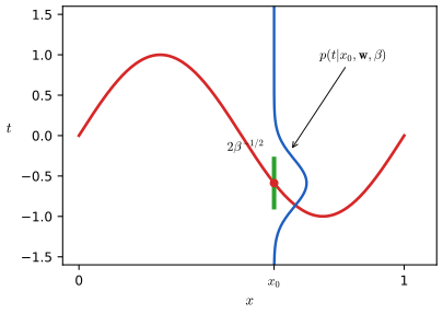
fig1_16() · in the notes · PDF · SVG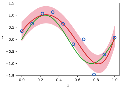
fig1_17() · in the notes · PDF · SVG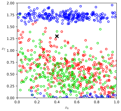
fig1_19() · in the notes · PDF · SVG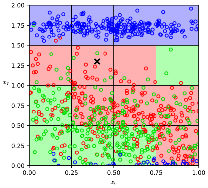
fig1_20() · in the notes · PDF · SVG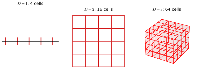
fig1_21() · in the notes · PDF · SVG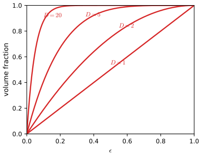
fig1_22() · in the notes · PDF · SVG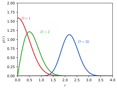
fig1_23() · in the notes · PDF · SVG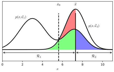
fig1_24() · in the notes · PDF · SVG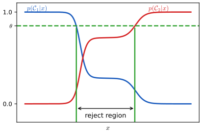
fig1_26() · in the notes · PDF · SVG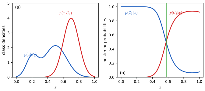
fig1_27() · in the notes · PDF · SVG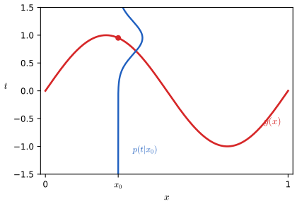
fig1_28() · in the notes · PDF · SVG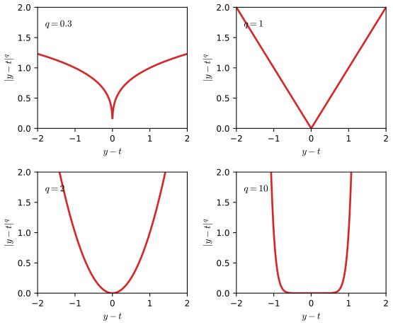
fig1_29() · in the notes · PDF · SVG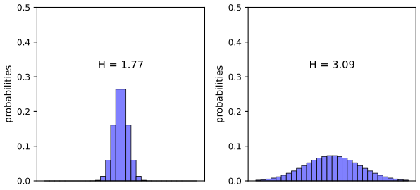
fig1_30() · in the notes · PDF · SVG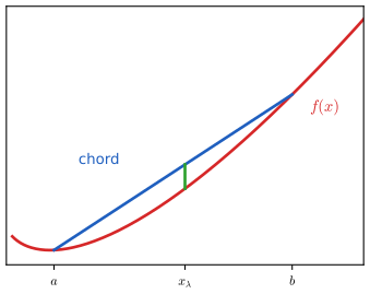
fig1_31() · in the notes · PDF · SVGChapter 2: Probability Distributions
Source: ch02_probability_distributions.py · run python3 ch02_probability_distributions.py --list to list its figures · lecture notes: ch02-probability-distributions.html
Module notes: data, settings and differences from the book
Bishop (2006), Chapter 2 (Probability Distributions): the algorithms and every numerical figure.
One function per figure (`python3 ch02_probability_distributions.py --list`); the building blocks (conjugate updates, Gaussian conditionals, Student t, von Mises, density estimators) are small documented functions that cite the book's equations and are also used by checks_ch02.py.
Choices and what could not be reproduced exactly (the book gives few numbers for this chapter): * Figure 2.1: N = 10, mu = 0.25 (stated in the text). Figures 2.2 and 2.13: the parameters printed in the panels. Figure 2.3: Beta(2, 2) prior and one observation x = 1 (stated in the caption). * Figure 2.5: Dirichlet with alpha_k = 0.1, 1, 10 (caption); the surface is drawn over the simplex (mu_1, mu_2) with mu_3 = 1 - mu_1 - mu_2 and a common height axis cut at 20. * Figure 2.6: 1000 draws of the mean of N uniform numbers, 20 bins. * Figure 2.9: a bivariate Gaussian with mean (0.5, 0.5), standard deviations 0.14 and correlation 0.95 (read off the marginal and conditional peaks 2.8 and 9 in the book's right-hand panel). * Figure 2.12: data from N(0.8, 0.1) (variance 0.1, caption), prior N(0, 0.1), likelihood variance 0.1; the first 1, 2, 10 points of one seeded sample. * Figure 2.14: normal-gamma with mu_0 = 0, beta = 2, a = 5, b = 6 (caption). * Figure 2.15: Student t with mu = 0, lambda = 1 and nu = 0.1, 1, infinity (caption). * Figure 2.16: 30 draws from N(0, 1) (a), then three outliers near 9 (b); the t fit is maximum likelihood by EM (mu, lambda) with nu from a one-dimensional maximisation of the EM bound. * Figure 2.19: m = 5, theta_0 = pi/4 and m = 1, theta_0 = 3 pi/4 (legend of the book's figure). * Figure 2.21: Old Faithful (272 points, common.old_faithful); a single Gaussian by maximum likelihood and a two-component mixture by EM started from the two ends of the data. * Figure 2.22: three one-dimensional Gaussians with weights 0.3, 0.3, 0.4 (shape read off the book; the values are ours). Figure 2.23: pi = (0.5, 0.3, 0.2), means (0.2, 0.4), (0.5, 0.5), (0.8, 0.6), covariance 0.016 [[1, r], [r, 1]] with r = 0.75, -0.75, 0.75 (read off the contours, as in Chapter 9). * Figures 2.24 to 2.26: 50 points from 0.35 N(0.3, 0.12^2) + 0.65 N(0.8, 0.1^2) (the book's green curve is not tabulated; this mixture has the same two peaks, heights about 1.2 and 2.6). * Figure 2.27: a small synthetic two-class set (the book's points are a sketch). * Figure 2.28: the first 200 points of the oil-flow training set (the book's subset is not stated), inputs x6 and x7, K = 1, 3, 31, ties broken at random (seeded), which gives the speckled ties of the book's K = 3 panel. * Figures 2.4, 2.7, 2.10, 2.17 and 2.18 are sketches and are not reproduced; Figure 2.11 is replaced by a real Robbins-Monro run (an addition, not in the book in this form).
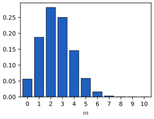
fig2_1() · in the notes · PDF · SVG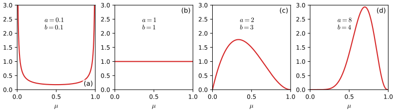
fig2_2() · in the notes · PDF · SVG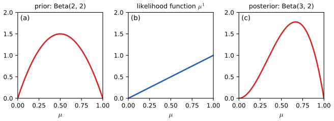
fig2_3() · in the notes · PDF · SVG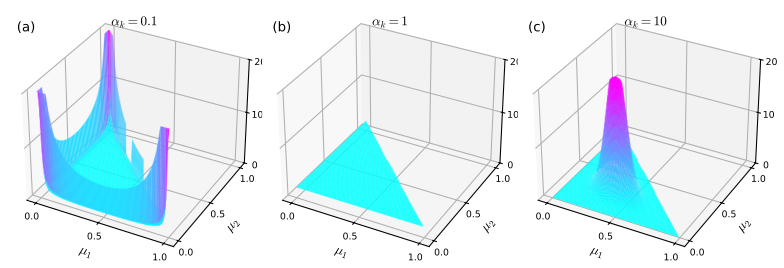
fig2_5() · in the notes · PDF · SVG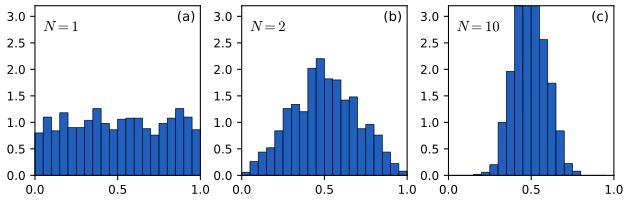
fig2_6() · in the notes · PDF · SVG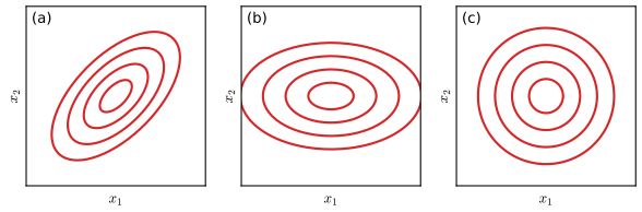
fig2_8() · in the notes · PDF · SVG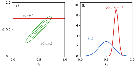
fig2_9() · in the notes · PDF · SVG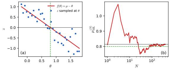
fig2_11() · in the notes · PDF · SVG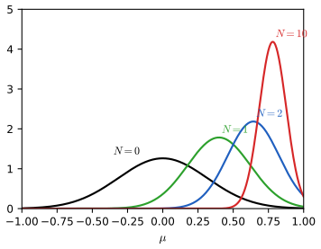
fig2_12() · in the notes · PDF · SVG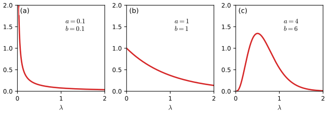
fig2_13() · in the notes · PDF · SVG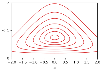
fig2_14() · in the notes · PDF · SVG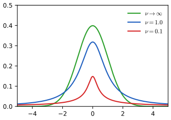
fig2_15() · in the notes · PDF · SVG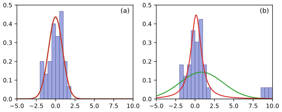
fig2_16() · in the notes · PDF · SVG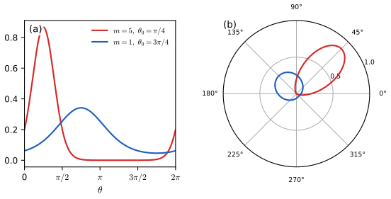
fig2_19() · in the notes · PDF · SVG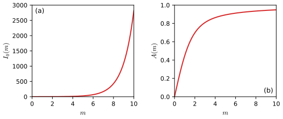
fig2_20() · in the notes · PDF · SVG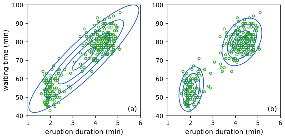
fig2_21() · in the notes · PDF · SVG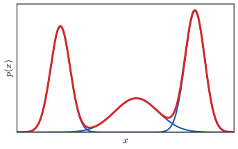
fig2_22() · in the notes · PDF · SVG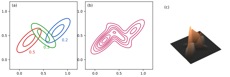
fig2_23() · in the notes · PDF · SVG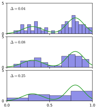
fig2_24() · in the notes · PDF · SVG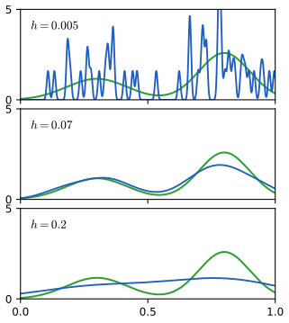
fig2_25() · in the notes · PDF · SVG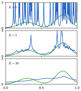
fig2_26() · in the notes · PDF · SVG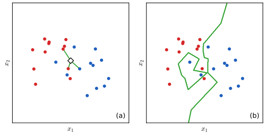
fig2_27() · in the notes · PDF · SVG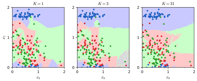
fig2_28() · in the notes · PDF · SVGChapter 3: Linear Models for Regression
Source: ch03_linear_regression.py · run python3 ch03_linear_regression.py --list to list its figures · lecture notes: ch03-linear-regression.html
Module notes: data, settings and differences from the book
Bishop (2006), Chapter 3: Linear Models for Regression.
Reproduces the numerical figures of Chapter 3 of C. M. Bishop, Pattern Recognition and Machine Learning (Springer, 2006), pp. 137-173, written from scratch with numpy, scipy and matplotlib. Every algorithm is a small function meant to be read next to the lecture notes (ch03-linear-regression.html):
* Section 3.1, basis functions: poly_basis, gauss_basis (3.4), sigmoid_basis (3.5), design_matrix. Section 3.1.1: ml_weights (the normal equations (3.15) solved by least squares, with noise precision (3.21)). Section 3.1.4: ridge_weights (3.28). * Section 3.1.3, sequential learning: lms_step (3.23). * Section 3.2, bias-variance: bias_variance (3.37)-(3.46) over L data sets. * Section 3.3, Bayesian linear regression: posterior (3.50)-(3.54), predictive (3.58)-(3.59), equivalent_kernel (3.60)-(3.62). * Sections 3.4 and 3.5, evidence: log_evidence (3.86), gamma_eff (3.91), evidence_update (3.92), (3.95), (3.98), evidence_iterate (the alpha/beta fixed point), evidence_path (alpha scanned).
Data. Everything is synthetic, as in the book: sin(2 pi x) plus Gaussian noise, with x uniform on (0, 1) (Section 1.1; Figures 3.5, 3.6, 3.8, 3.9, 3.14, 3.16, 3.17), or the line a0 + a1 x with a0 = -0.3, a1 = 0.5, noise standard deviation 0.2 and x uniform on (-1, 1) (Figure 3.7, as in the text). Random numbers come from JSRandom (the seeded generator DK.rng of the browser demos), so the demos bayesian-regression-demo.html, bias-variance-demo.html and evidence-demo.html draw the same data number for number.
Figures: 3.1 to 3.11, 3.14 to 3.17 (3.12 and 3.13 are schematic sketches, not reproduced). Run `python3 ch03_linear_regression.py --list`, `python3 ch03_linear_regression.py` (all figures, about half a minute) or `--fig 3.7 3.8`. Files go to ../img/ch03/.
Settings chosen where the book gives none, and what differs: * Figure 3.1: polynomials x^1..x^10, Gaussians (3.4) with s = 0.2 centred at -1, -0.8, ..., 1, and sigmoids (3.5) with s = 0.1 and the same centres. * Figure 3.2: N = 3 observations, M = 2 basis functions, in 3-d (the book's sketch, with numbers). * Figure 3.3: the contours |w1|^q + |w2|^q = 1. Figure 3.4: the contours of a quadratic error centred at w_ML = (1.1, 0.55) with the constraint region |w1|^q + |w2|^q <= 0.8; the optimum w* is computed numerically (the lasso optimum has w1 = 0). * Figures 3.5 and 3.6: L = 100 data sets of N = 25 points, noise standard deviation 0.3, 24 Gaussian basis functions (s = 0.1, centres equally spaced on [0, 1]) plus a bias, ridge regression (3.28), ln lambda = 2.6, -0.31, -2.4 for Figure 3.5. The bias and variance integrals are taken over a grid of 200 equally spaced x on [0, 1], the density p(x) being uniform. The book's curves are lower than ours for the test error: its test error is about 0.065 whereas bias^2 + variance + sigma^2 here is about 0.1 for sigma = 0.3; the book's value is consistent with a noise variance of about 0.05, so we cannot recover its exact test noise. Our test error is bias^2 + variance + sigma^2, computed on 1000 fresh points per data set (it agrees with that sum to Monte Carlo accuracy). * Figures 3.8 and 3.9: 9 Gaussian basis functions (s = 0.1, centres equally spaced on [0, 1]) plus a bias, alpha = 2, beta = 25 (noise standard deviation 0.2), N = 1, 2, 4, 25. * Figures 3.10 and 3.11: alpha = 0.005, beta = 11.1; 200 equally spaced x on (-1, 1); the basis functions of Figure 3.1. * Figure 3.14: N = 10 points x = 0, 1/9, ..., 1, noise standard deviation 0.3 (beta = 1/0.09), alpha = 5e-3 as in the text; polynomial orders M = 0..8. * Figures 3.16 and 3.17: N = 25 points, noise standard deviation 0.3, 9 Gaussian basis functions (s = 0.1) plus a bias (10 parameters), beta fixed at 1/0.09. Figure 3.16(c) is an addition: the iteration (3.92)/(3.95)/(3.98) of alpha and beta from alpha = beta = 1. * Figure 3.15 is computed for a two-parameter example (a Hessian with eigenvalues 1 and 9).
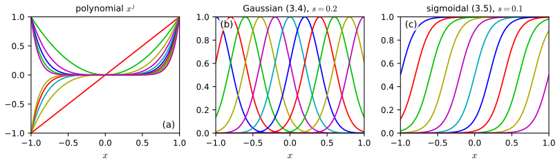
fig3_1() · in the notes · PDF · SVG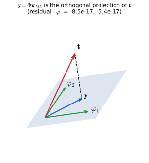
fig3_2() · in the notes · PDF · SVG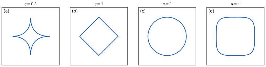
fig3_3() · in the notes · PDF · SVG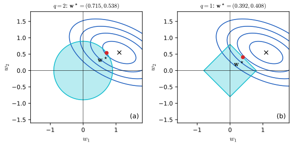
fig3_4() · in the notes · PDF · SVG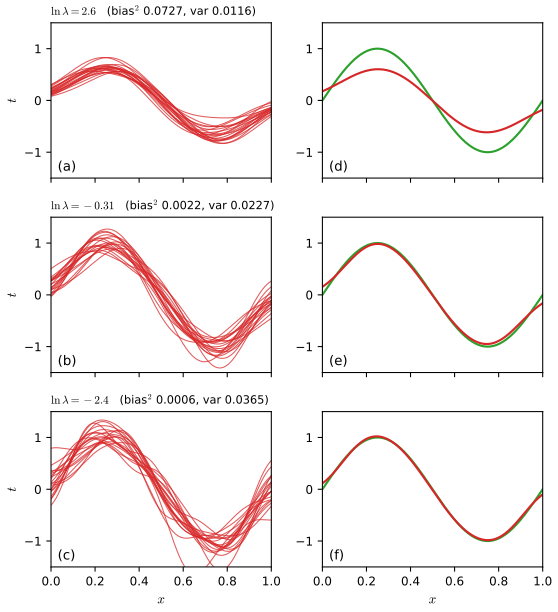
fig3_5() · in the notes · PDF · SVG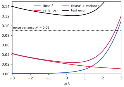
fig3_6() · in the notes · PDF · SVG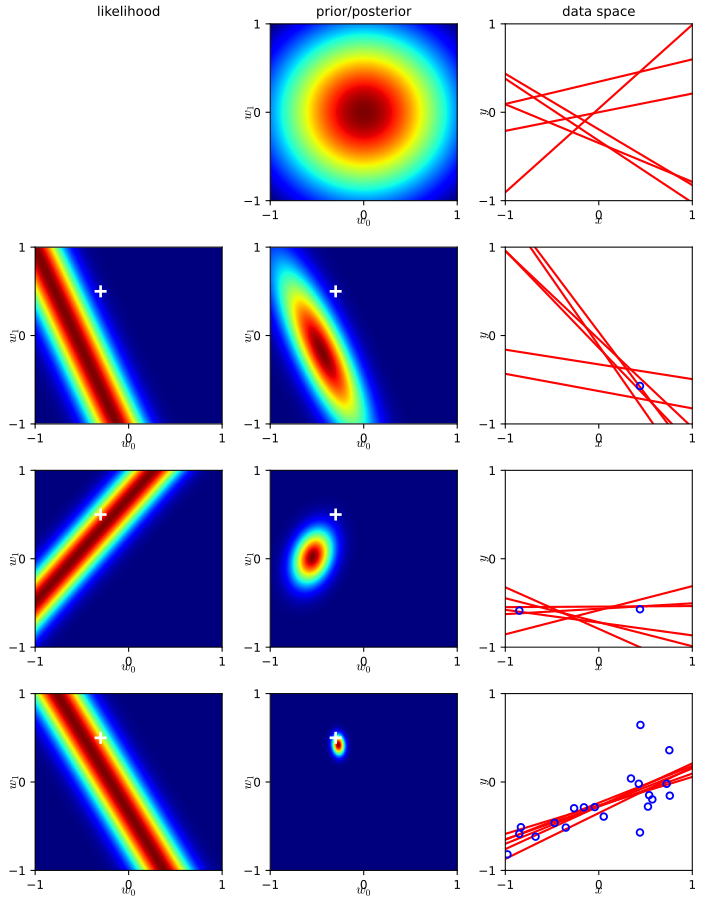
fig3_7() · in the notes · PDF · SVG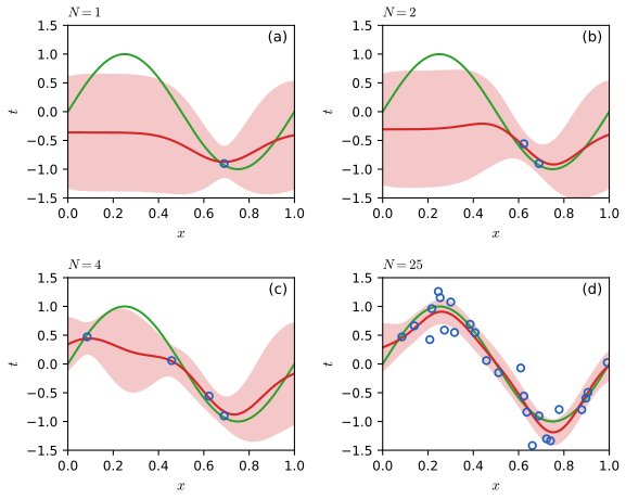
fig3_8() · in the notes · PDF · SVG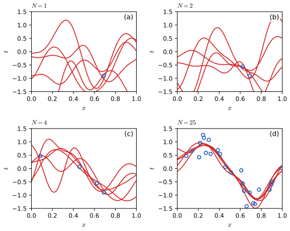
fig3_9() · in the notes · PDF · SVG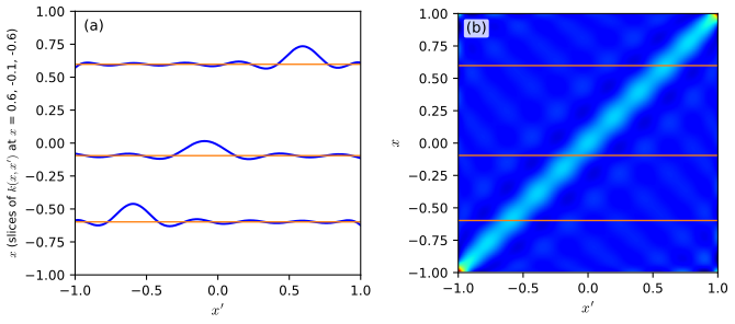
fig3_10() · in the notes · PDF · SVG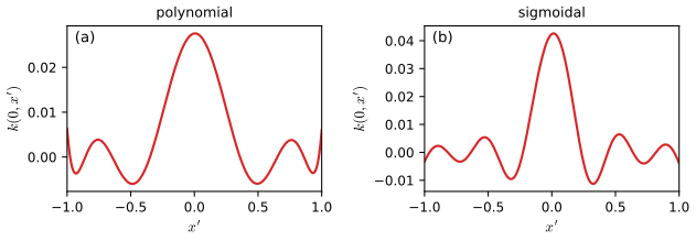
fig3_11() · in the notes · PDF · SVG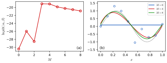
fig3_14() · in the notes · PDF · SVG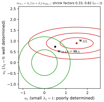
fig3_15() · in the notes · PDF · SVG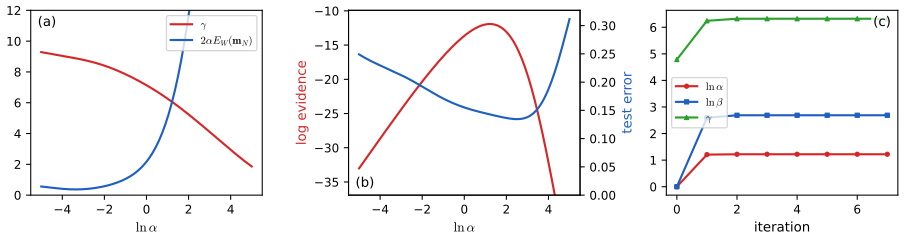
fig3_16() · in the notes · PDF · SVG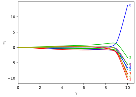
fig3_17() · in the notes · PDF · SVGChapter 4: Linear Models for Classification
Source: ch04_linear_classification.py · run python3 ch04_linear_classification.py --list to list its figures · lecture notes: ch04-linear-classification.html
Module notes: data, settings and differences from the book
Bishop (2006), Chapter 4: Linear Models for Classification.
Reproduces the numerical figures of Chapter 4 of C. M. Bishop, Pattern Recognition and Machine Learning (Springer, 2006), pp. 179-224, written from scratch with numpy, scipy and matplotlib. Every algorithm is a small function meant to be read next to the lecture notes (ch04-linear-classification.html):
* Section 4.1, discriminant functions: least_squares_classifier (the pseudo-inverse solution (4.16)), fisher_two_class ((4.28)-(4.30)), fisher_criterion ((4.25)-(4.27)), fisher_multiclass ((4.40)-(4.50), eigenvectors of S_W^-1 S_B), perceptron ((4.54)-(4.55), cycling through the data). * Section 4.2, probabilistic generative models: gaussian_generative_fit (maximum likelihood (4.75)-(4.80), shared covariance) and generative_posterior (the logistic sigmoid (4.57)-(4.67) for two classes, the softmax (4.62)-(4.65) for K classes). * Section 4.3, probabilistic discriminative models: logistic_loglik, logistic_grad_hess ((4.90)-(4.97)), irls_logistic (Newton-Raphson, the weighted least-squares form (4.99)-(4.101), optional L2 term), softmax and multiclass_irls ((4.104)-(4.110)), probit_irls (Fisher scoring for the inverse probit link (4.114)-(4.116)). * Section 4.4, Laplace approximation: laplace_1d ((4.125)-(4.127)), laplace_logistic (the Gaussian posterior (4.142)-(4.143), the evidence (4.137) and the BIC (4.139)). * Section 4.5.2, the predictive distribution: bayes_predictive ((4.150)-(4.155), the probit approximation sigma(a) ~ Phi(lambda a) with lambda^2 = pi/8 and kappa(sigma^2)). * JSRandom (imported from ch11_sampling.py): the seeded generator DK.rng of the browser demos. The data sets below (blobs, make_two_class, make_three_class, make_fisher_data) draw from JSRandom in a fixed order, so linear-classifiers-demo.html and logistic-regression-demo.html reproduce the same points number for number.
Figures: 4.1, 4.2, 4.3, 4.4, 4.5, 4.6, 4.7, 4.9, 4.10, 4.11, 4.12, 4.13, 4.14. Run `python3 ch04_linear_classification.py --list`, `python3 ch04_linear_classification.py` (all figures, under a minute) or `python3 ch04_linear_classification.py --fig 4.4 4.6`. Files go to ../img/ch04/. Not reproduced: Figure 4.8 (a photograph of the Mark 1 perceptron).
The book states the settings of its synthetic data only in the figures. What we chose (and what we did not copy) is listed here: * Figure 4.4: two Gaussian classes in the plane, 40 points each. Red (x): mean (-1.3, 1.3), standard deviations (1.2, 1.0), correlation 0.3; blue (o): mean (1.0, -1.6), standard deviations (0.9, 1.2), correlation 0.7. The right panel adds 10 blue points around (7.7, -6) (standard deviations 0.5, correlation 0). The least-squares boundary is the line where the two fitted outputs y_1(x) = y_2(x) agree; logistic regression is fitted by IRLS (4.99). * Figure 4.5: three Gaussian classes, 40 points each: red (-2.5, 2.3), sd (1.3, 1.2), rho 0.3; green (-0.4, 0), sd (1.0, 1.0), rho 0.8 (a strip along the diagonal between the other two); blue (2.0, -2.2), sd (1.1, 1.0), rho 0.3. The multiclass logistic regression of the right panel uses IRLS (4.109)-(4.110) with a tiny L2 term (alpha = 1e-4). * Figure 4.6: two classes with the same covariance (sd (1.3, 0.45), correlation 0.3), blue mean (1.0, 3.0), red mean (3.8, 1.5), 100 points each. The left panel projects onto the line joining the class means, the right panel onto the Fisher direction (4.30). * Figure 4.7: the eight-point-like data set is read off the book: five red points (+1) at (0.23, 0.72), (0.45, 0.30), (0.97, 0.90), (0.37, -0.49), (0.66, -0.90) and five blue points (-1) at (-0.75, 0.95), (-0.77, 0.61), (-0.55, 0.64), (-0.40, 0.73), (-0.10, -0.20); features phi = x without a bias, initial w = (-0.42, -0.90), points visited in this order, continuing cyclically after the last update. The sequence of updates then is the book's two (the figure's panels (a)-(d)). * Figure 4.9: sigma(a) and Phi(lambda a) with lambda^2 = pi/8 (an exact reproduction). * Figure 4.10: two Gaussian classes with means (-0.55, 0) and (0.55, 0), the shared covariance diag(0.4^2, 0.5^2) and equal priors (FIG10); surfaces are drawn with matplotlib's 3-D axes. The left surface is p(x|C_k) p(C_k) coloured by the posterior. * Figure 4.11: three Gaussian classes: red (-1, -1) and green (-1, 1) share the covariance diag(0.3^2, 0.2^2); blue (1.5, 0) has diag(0.12^2, 0.32^2); equal priors; contours at 1, 2, 3 standard deviations (in the right panel the RGB colour is the posterior vector). * Figure 4.12: red cluster N((0, 0), 0.3^2 I) and two blue clusters around (-1.1, -0.95) and (0.95, 1.05); two Gaussian basis functions with centres (-1, -1) and (0, 0), width 0.78; logistic regression in the (phi_1, phi_2) plane (alpha = 0.01). * Figure 4.13 is a schematic in the book (a mixture of two Gaussians and its cumulative distribution); we compute it (weights 0.7, 0.3; means 1.5, 3.0; sd 0.4, 0.3). * Figure 4.14: exactly the book's p(z) proportional to exp(-z^2/2) sigma(20 z + 4). The mode is z_0 = 0.0775 and the exact curvature -d^2 ln f/dz^2 = 1 + 400 sigma(1 - sigma) = A = 2.54 (checked by finite differences in checks_ch04.py), so the Gaussian has peak sqrt(A / 2 pi) = 0.64. The red curve printed in the book is narrower (peak about 0.76, which corresponds to A of about 3.6); we plot the exact Laplace approximation, and the yellow density agrees with the book's. * Figures 4.1, 4.2, 4.3 are geometric drawings in the book; they are drawn here from computed discriminants (planes, one-versus-the-rest, one-versus-one, the convex decision regions).
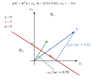
fig4_1() · in the notes · PDF · SVG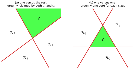
fig4_2() · in the notes · PDF · SVG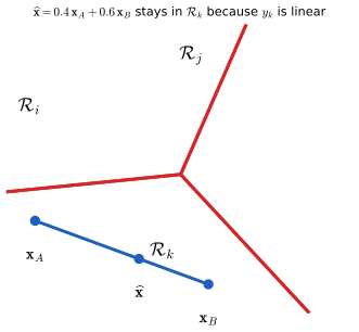
fig4_3() · in the notes · PDF · SVG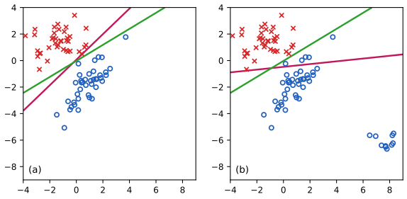
fig4_4() · in the notes · PDF · SVG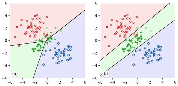
fig4_5() · in the notes · PDF · SVG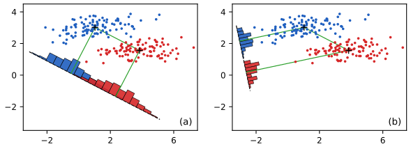
fig4_6() · in the notes · PDF · SVG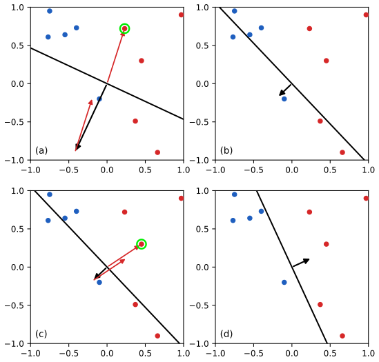
fig4_7() · in the notes · PDF · SVG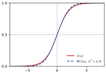
fig4_9() · in the notes · PDF · SVG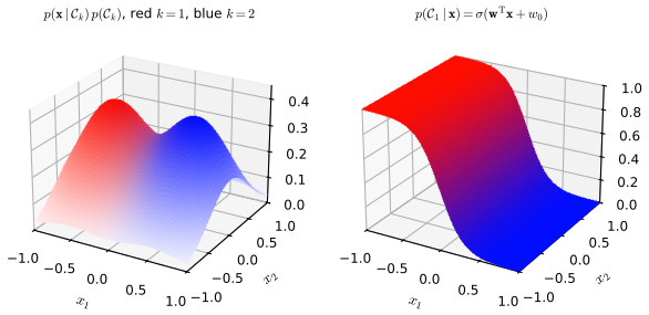
fig4_10() · in the notes · PDF · SVG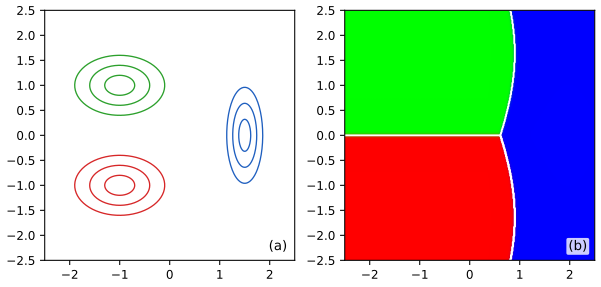
fig4_11() · in the notes · PDF · SVG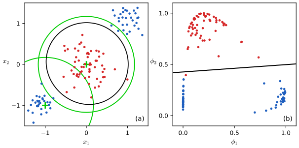
fig4_12() · in the notes · PDF · SVG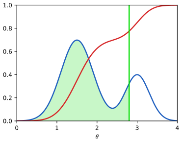
fig4_13() · in the notes · PDF · SVG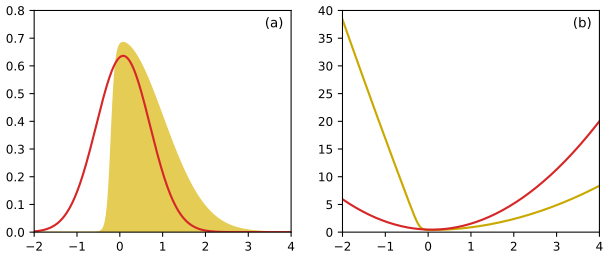
fig4_14() · in the notes · PDF · SVGChapter 5: Neural Networks
Source: ch05_neural_networks.py · run python3 ch05_neural_networks.py --list to list its figures · lecture notes: ch05-neural-networks.html
Module notes: data, settings and differences from the book
Bishop (2006), Chapter 5: Neural Networks.
Reproduces the numerical figures of Chapter 5 of C. M. Bishop, Pattern Recognition and Machine Learning (Springer, 2006), pp. 225-290, written from scratch with numpy, scipy and matplotlib. Every algorithm is a small function meant to be read next to the lecture notes (ch05-neural-networks.html):
* Section 5.1, feed-forward network functions: Net (any number of layers of tanh hidden units; output units linear, logistic sigmoid or softmax (5.1)-(5.9); the weights and biases are one flat vector w, so w = (hidden-unit biases and weights, then output-unit biases and weights)). * Sections 5.2-5.3, error functions and backpropagation: the sum-of-squares, cross-entropy and multiclass cross-entropy errors (5.11), (5.21), (5.24) all give the output delta y - t for the canonical link (5.18), (5.66), (5.69); Net.backward is (5.43)-(5.56); a mixture density network has its own error (5.153) and derivatives (5.155)-(5.157) (with the errata). * Section 5.3.4, the Jacobian: Net.jacobian is (5.72)-(5.76). * Section 5.4, the Hessian: hessian_diagonal ((5.79)-(5.81), the exact diagonal of Ricotti et al. and the Becker-Le Cun approximation), hessian_outer ((5.83)-(5.85), outer product / Levenberg- Marquardt), inverse_hessian_sequential ((5.86)-(5.89)), hessian_fd ((5.91)), hessian_exact (the two-layer formulas (5.92)-(5.95)), hessian_vector (the R-operator (5.96)-(5.108), for any depth) and hessian_rop (the full Hessian from W Hessian-vector products). * Section 5.5, regularisation: weight decay (5.112), early stopping in a quadratic error (Figure 5.13, early_stopping_vs_weight_decay), warped digits (Figure 5.14, warp_digit) and tangent vectors (Figure 5.16, rotate_tangent). * Section 5.6, mixture density networks: mdn_error, mdn_delta, mdn_parameters, mdn_mode. * Section 5.7, Bayesian neural networks (Laplace approximation, MacKay's evidence framework): laplace_log_evidence_regression (5.175), evidence_regression (alternating a fit of w with (5.178)-(5.182)), predictive_regression ((5.172)-(5.173)), evidence_classification ((5.183)-(5.186)), predictive_classification ((5.188)-(5.190)). * JSRandom (imported from ch11_sampling.py): the seeded generator DK.rng of the browser demos. data_sine, init_weights and adam_train below use only that generator's numbers and plain floating-point arithmetic, so backprop-demo.html, mixture-density-demo.html and bayesian-nn-demo.html reproduce them number for number (see the checks in the demos' pages).
Figures: 5.3, 5.4, 5.9, 5.10, 5.11, 5.12, 5.13, 5.14, 5.16, 5.19, 5.21, 5.22, 5.23 (the book's other figures in this chapter are diagrams). Run `python3 ch05_neural_networks.py --list`, `python3 ch05_neural_networks.py` (all figures, a few minutes) or `python3 ch05_neural_networks.py --fig 5.3 5.21`. Files go to ../img/ch05/.
What differs from the book, and the settings chosen where the book gives none: * Optimiser: the book uses scaled conjugate gradients; we use L-BFGS (scipy) for the figures, from several random starts when the error has bad local minima (we keep the best), and Adam or plain gradient descent in the demos. Any local minimiser reaches the same kind of solution. * Figure 5.3: N = 50 points uniform on (-1, 1) (we use an equally spaced grid), no noise, three tanh hidden units, linear output. The caption says f(x) = sin(x), but on (-1, 1) that is almost a straight line; the book's panel (b) shows one full hump, so we use sin(2x), whose maximum is at x = 0.785; the dashed curves are the three hidden-unit outputs z_j(x) (the book draws them rescaled to fit). * Figure 5.4: the synthetic classification data of Appendix A are not published, so we draw 100 points (50 per class; JSRandom(3)) from our own version of its generative process: blue class N((-0.2, 0.0), diag(1.0^2, 1.2^2)), red class an equal mixture of N((1.0, 1.1), diag(0.6^2, 0.8^2)) and N((0.9, -1.1), diag(0.6^2, 0.7^2)); see classification_data. The green curve is the 0.5 contour of the true posterior. The dashed blue lines are a_j = 0 for each hidden unit, i.e. where z_j = tanh(a_j) = 0 (the book's caption says 0.5, which is not the midpoint of tanh). * Figures 5.9 and 5.10: data from the sinusoid of Appendix A (x uniform on (0, 1), t = sin(2 pi x) plus noise with sd 0.3). Figure 5.9 uses the ten points x_n = (n - 1)/9 so that all three panels see the same data (as in the book), and the best of 8 starts of L-BFGS on the sum of squares plus a tiny weight decay (lambda = 1e-3), which only stops the weights of the over-flexible networks running off to huge values (without it the M = 3 and M = 10 fits contain near-vertical spikes between the points). Figure 5.10 uses 60 training points and a test set of 600 (L-BFGS, at most 1500 iterations, a few starts end far above the plotted range), reports the sum of squares sum (y - t)^2 on the test set (floor 600 x 0.09 = 54), and initialises each of the 30 starts per M with weights N(0, 10), as stated in the caption. * Figure 5.11: the book's panel titles give the precisions with an erratum: every number on the right of '=' should be raised to the power -2. So panels are (a) all alphas 1, (b) alpha2w = 10^-2, (c) alpha1w = 10^-6, alpha1b = 10^-4, (d) alpha1w = alpha1b = 10^-6. 12 tanh hidden units, five prior draws per panel. * Figure 5.12: 12 training and 12 validation points of the sinusoid (numpy seed 25), a network with 10 hidden units, plain full-batch gradient descent (step 0.004) from a small random start (N(0, 0.5^2)); the curves show the RMS error sqrt(2 E / N) after every 400 gradient steps (50 values), and the dashed line marks the minimum of the validation error. (The book's units are not stated; RMS error has the right scale.) * Figure 5.13: a quadratic error with Hessian eigenvalues 1 and 0.05 (read off the book's ellipse); the curve is the gradient-descent path from the origin, and the dotted curve the ridge path w(alpha) for weight decay. Both are computed in closed form. * Figure 5.14: the digit is MNIST test image 0 of class 6 (MNIST digits are the book's 'off-line digits'). The book smooths i.i.d. random displacements with Gaussians of width 0.01, 30 and 60 on a larger image. On our 28 x 28 images we use widths 0.01, 2.5 and 5 pixels, and rescale each field to an rms displacement of 1.2 pixels (0.6 pixels for the unsmoothed field), displacements drawn uniformly in (-1, 1) before smoothing; the warp is a cubic-spline resampling. * Figure 5.16: tangent vector tau = d x(xi)/d xi at xi = 0 for rotation by xi (central finite difference of the cubic-spline rotated image), x + epsilon tau with epsilon = 15 degrees = 0.262 rad, and the truly rotated image (clockwise, as in the book). * Figures 5.19 and 5.21: x uniform on (0, 1), t = x + 0.3 sin(2 pi x) + noise uniform on (-0.1, 0.1), N = 250 points; the inverse problem swaps x and t. The network of 5.19 has five tanh hidden units and the sum-of-squares error; the mixture density network has three Gaussian components, five hidden units and 9 outputs (the book's own numbers). In panel (d) the conditional mode is approximated, as in the book, by the mean of the most probable component. * Figures 5.22 and 5.23: our version of the classification data of Figure 5.4 with N = 100, a network with 8 tanh hidden units, a single hyperparameter alpha started at 0 as in the caption (we start at alpha = 0.01 to keep the Hessian well-conditioned), re-estimated by the evidence procedure (5.178)-(5.179) alternating with the fit of w, as in evidence_classification.
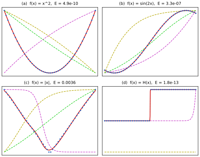
fig5_3() · in the notes · PDF · SVG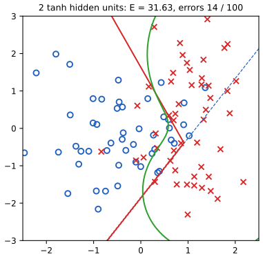
fig5_4() · in the notes · PDF · SVG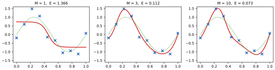
fig5_9() · in the notes · PDF · SVG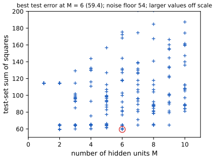
fig5_10() · in the notes · PDF · SVG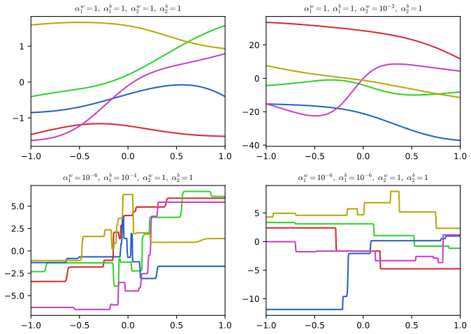
fig5_11() · in the notes · PDF · SVG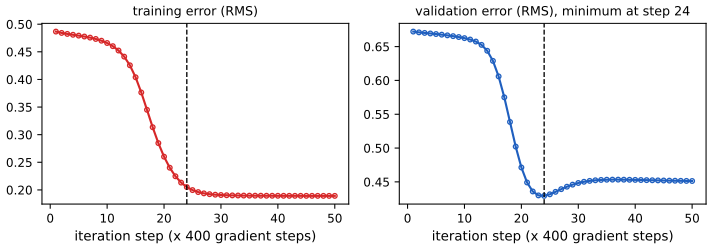
fig5_12() · in the notes · PDF · SVG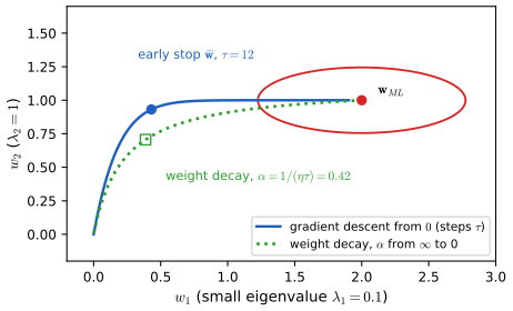
fig5_13() · in the notes · PDF · SVG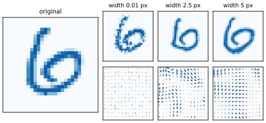
fig5_14() · in the notes · PDF · SVG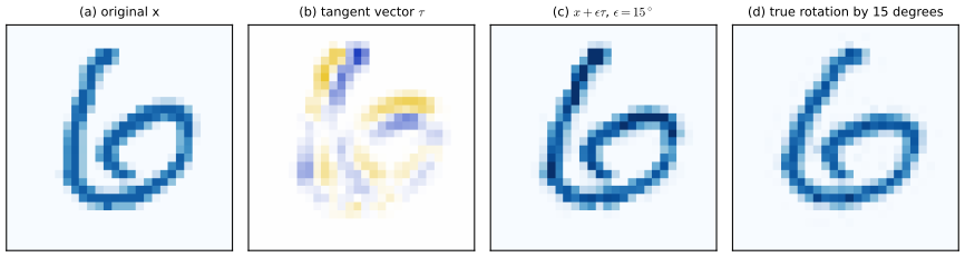
fig5_16() · in the notes · PDF · SVG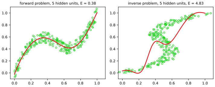
fig5_19() · in the notes · PDF · SVG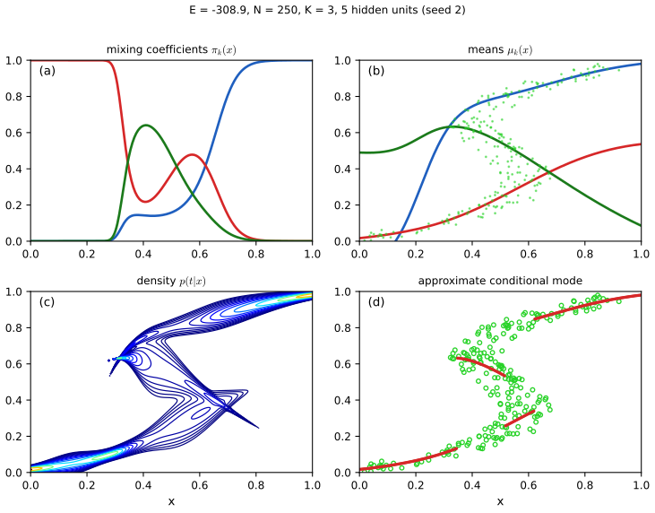
fig5_21() · in the notes · PDF · SVG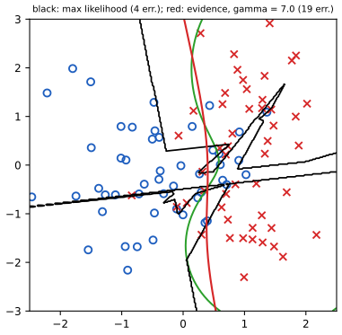
fig5_22() · in the notes · PDF · SVG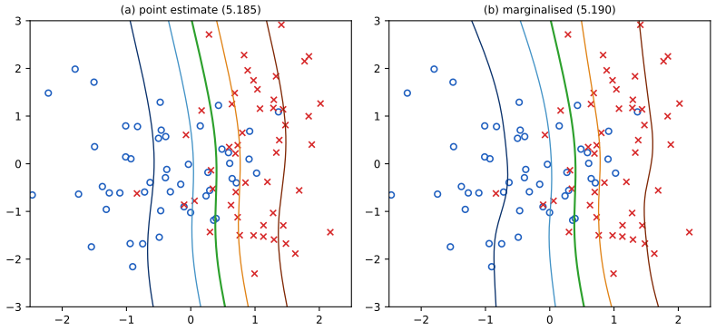
fig5_23() · in the notes · PDF · SVGChapter 6: Kernel Methods
Source: ch06_kernel_methods.py · run python3 ch06_kernel_methods.py --list to list its figures · lecture notes: ch06-kernel-methods.html
Module notes: data, settings and differences from the book
Bishop (2006), Chapter 6: Kernel Methods.
Reproduces the numerical figures of Chapter 6 of C. M. Bishop, Pattern Recognition and Machine Learning (Springer, 2006), pp. 291-323, written from scratch with numpy, scipy and matplotlib. Every algorithm is a small function meant to be read next to the lecture notes (ch06-kernel-methods.html):
* Section 6.1, dual representations: ridge_primal and ridge_dual (the dual solution a = (K + lambda I)^(-1) t of (6.8) and the prediction (6.9)). * Section 6.2, constructing kernels: kernels from basis functions (6.10) (basis_kernel), the polynomial kernel (6.12), the Gaussian kernel (6.23), the sigmoidal kernel (6.37), the closure rules (6.13)-(6.22) (see checks_ch06.py) and the exponential kernel (6.56). * Section 6.3, radial basis functions: normalised basis functions (6.41) and the Nadaraya-Watson model (6.45)-(6.48) with its Gaussian-mixture conditional density (nadaraya_watson). * Section 6.4, Gaussian processes: kernel classes with analytic derivatives (GaussKernel, ExpKernel; the covariance (6.63) and the ARD kernel (6.71)-(6.72)), gp_predict ((6.66)-(6.67)), gp_log_marginal ((6.69) and its gradient (6.70)), gp_fit (maximum marginal likelihood by L-BFGS), and GP classification with the Laplace approximation: laplace_mode (Newton-Raphson (6.83), fixed point (6.84)), laplace_predict ((6.87)-(6.88) and (4.153)) and laplace_evidence ((6.90) with the gradient (6.91)-(6.94)).
Figures (the code builds every numerical figure of the chapter): 6.1 to 6.12. Choices made where the book does not say (the functions are chosen to look like the book's, not copied):
* 6.1: polynomial basis x^j, j = 1..10; 21 Gaussian basis functions of width 0.1 spaced 0.1 apart (every second one is drawn in the top panel; the kernel uses all 21, which gives the peak height 1.77 of the book); 11 logistic sigmoids sigma((x - mu)/0.1) spaced 0.2 apart (peak 5.5 as in the errata-corrected figure). Kernel plotted against x with x' = -0.5, 0, 0. * 6.2: three Gaussian basis functions with centres -0.5, 0.1, 0.65 and widths 0.1, 0.13, 0.25 (read off the figure). * 6.3: the sinusoidal data set of Appendix A with N = 10 equally spaced inputs, noise sd 0.3 (seeded), Gaussian kernel sd 0.1. * 6.4, 6.5: prior samples on [-1, 1]; the same standard-normal draws are used in every panel (like the book, where the panels are visibly related). Exponential kernel with theta = 4. * 6.6: Gaussian kernel (theta0, theta1) = (1, 4), noise sd 0.5, 12 random inputs. * 6.7: correlation 0.5 between the two function values, t1 = 0.95. * 6.8: the first 7 of N = 10 equally spaced points of the sinusoidal data (the three right-most omitted, as in the book), kernel (6.63) with theta0 = 1, theta1 = 12, beta^(-1) = 0.3^2. * 6.9: ARD prior samples with the stated eta, drawn over [-4, 4]^2 (the book's wiggles imply a larger input range than the tick labels show). * 6.10: the book's recipe (x1 Gaussian, t = sin(2 pi x1) + noise, x2 = x1 + noise, x3 independent Gaussian) with our own scales; the marginal likelihood is maximised by L-BFGS-B (100 iterations) instead of scaled conjugate gradients, so the curves differ in detail. * 6.11: a sample of a(x) from a GP with Gaussian kernel (theta0 = 16, theta1 = 16) and sigma(a). * 6.12: the book's data set (Appendix A, Figure A.7) is not available, so a synthetic two-class set of the same type is made (blue: one Gaussian; red: mixture of two Gaussians; equal priors, 100 points each); the kernel amplitude and length scale are learnt by maximising the Laplace evidence (6.90) with the analytic gradient.
Run `python3 ch06_kernel_methods.py --list` for the figure list.
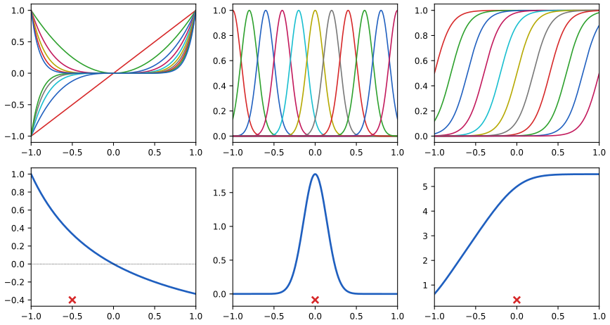
fig6_1() · in the notes · PDF · SVG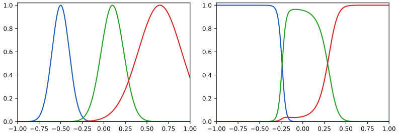
fig6_2() · in the notes · PDF · SVG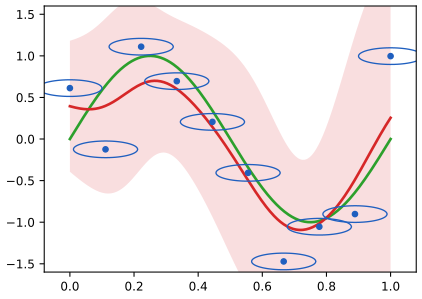
fig6_3() · in the notes · PDF · SVG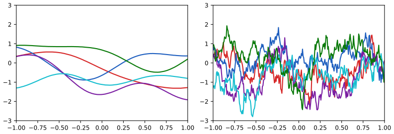
fig6_4() · in the notes · PDF · SVG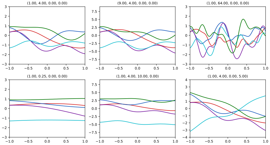
fig6_5() · in the notes · PDF · SVG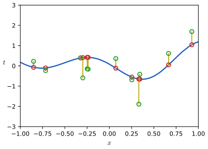
fig6_6() · in the notes · PDF · SVG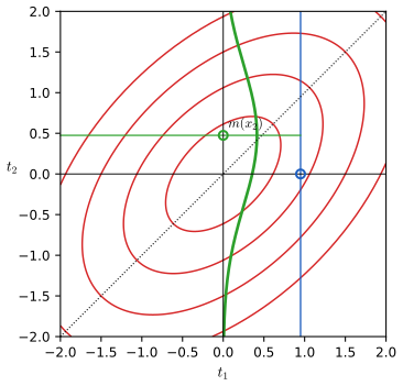
fig6_7() · in the notes · PDF · SVG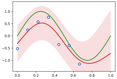
fig6_8() · in the notes · PDF · SVG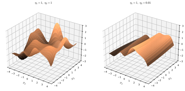
fig6_9() · in the notes · PDF · SVG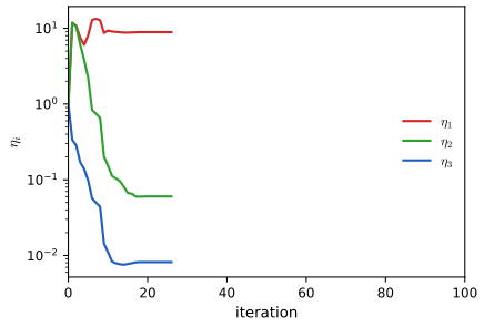
fig6_10() · in the notes · PDF · SVG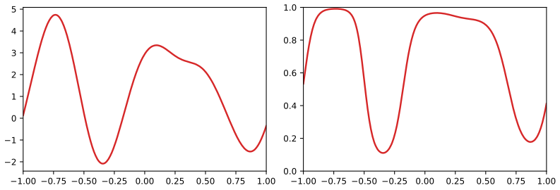
fig6_11() · in the notes · PDF · SVG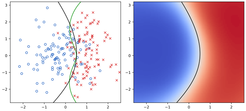
fig6_12() · in the notes · PDF · SVGChapter 7: Sparse Kernel Machines
Source: ch07_sparse_kernel_machines.py · run python3 ch07_sparse_kernel_machines.py --list to list its figures · lecture notes: ch07-sparse-kernel-machines.html
Module notes: data, settings and differences from the book
Bishop (2006), Chapter 7: Sparse Kernel Machines.
Reproduces the numerical figures of Chapter 7 of C. M. Bishop, Pattern Recognition and Machine Learning (Springer, 2006), pp. 325-358, written from scratch with numpy and matplotlib (no optimisation library is used at all). Every algorithm is a small function meant to be read next to the lecture notes (ch07-sparse-kernel-machines.html):
* Section 7.1, support vector machines. smo_solve is one sequential-minimal-optimisation solver (Platt 1999, with the second-order working-set rule of Fan, Chen and Lin 2005) for the dual quadratic programme min 1/2 a'Qa + p'a s.t. y'a = 0, 0 <= a <= C. It is used four ways: - svc_fit: hard-margin (C = infinity, dual (7.32)-(7.34)) and soft-margin (C finite, dual (7.43)-(7.45)) classification, decision function (7.13) and (7.37), b from (7.37) averaged over the unbounded support vectors; - nu_svc_fit: the nu-SVM (7.49)-(7.52), obtained as the C-SVM whose support-vector fraction is nu (Scholkopf et al. 2000: the two formulations have the same solutions); - svr_fit: epsilon-insensitive regression, dual (7.61)-(7.63) with coefficients (a_n - a^_n) as in (7.64), written as one 2N-variable problem with y = (+1,...,+1,-1,...,-1); - nu_svr_fit: the nu-SVR (7.68)-(7.72), again as the epsilon-SVR whose support-vector fraction is nu. The primal and dual objectives, the margin 1/||w|| and the KKT residuals are returned so that checks_ch07.py can verify them. * Section 7.2, relevance vector machines. rvm_regression is the evidence-maximising RVM: the posterior (7.81)-(7.83), the re-estimation equations (7.87)-(7.89) (MacKay updates) or the EM updates, pruning of basis functions whose alpha_i diverges; log_evidence_direct (7.85)-(7.86) and log_evidence_woodbury (the same number from the M x M matrices, (3.86)) are two routes to the marginal likelihood. rvm_fast_regression is the sequential sparse Bayesian learning algorithm of Section 7.2.2 (sparsity s_i and quality q_i, (7.97)-(7.101), Faul and Tipping 2002), whose log marginal likelihood never decreases. rvm_classification is Section 7.2.3: IRLS for the mode (7.110)-(7.112), the Laplace covariance (7.113), the evidence (7.114) and the update (7.116).
Figures: 7.1, 7.2, 7.4, 7.5, 7.6, 7.8, 7.9, 7.10, 7.11, 7.12 (7.3 and 7.7 are pure sketches of slack variables and are not reproduced). Run `python3 ch07_sparse_kernel_machines.py --list`, `python3 ch07_sparse_kernel_machines.py` (all figures, a few seconds) or `--fig 7.2 7.12`. Files go to ../img/ch07/.
What differs from the book, and the settings chosen where the book gives none: * The book's synthetic data (Appendix A) are not distributed with it. Three stand-ins are used, all generated with seeded numpy generators: - Figures 7.1 and 7.2: a small separable two-class set (Fig. 7.2: a blue Gaussian blob inside a red ring, 14 + 18 points, rejection-sampled so that the classes are separable; Gaussian kernel exp(-gamma ||x - x'||^2), gamma = 0.8, hard margin as the figure shows no slack). - Figures 7.4 and 7.12: the Ripley-type data of Appendix A (each class an equal mixture of two Gaussians, centres (-0.7, 0.3), (0.3, 0.3) and (-0.3, 0.7), (0.4, 0.7), standard deviation 0.25, which overlap heavily), 100 points per class, shifted and scaled to zero mean and unit standard deviation per axis (the book's plot has axes about -2.3 to 2.6). Fig. 7.4: nu-SVM with nu = 0.5 and Gaussian kernel gamma = 0.45 (the book's gamma; its nu is not stated). Fig. 7.12: RVM with the Gaussian kernel exp(-gamma||x-x'||^2), gamma = 0.45 as well. - Figures 7.8 and 7.9: ten points t = sin(2 pi x) + N(0, 0.2^2) at x = 0, 1/9, ..., 1 (seed 3), Gaussian kernel exp(-gamma (x-x')^2), gamma = 15 for the nu-SVR (nu = 0.7, C = 5) and the RVM (the book states only 'the same Gaussian kernel functions'). * The nu-SVM is solved as a C-SVM with C found by bisection so that the support-vector fraction equals nu; at the solution the margin-error fraction is at most nu, as (7.50)-(7.52) require. * Figure 7.10 is a schematic in the book; here it is computed with a chosen t and phi. * Figure 7.11 plots (7.97) for (q^2, s) = (4, 1) and (1, 2).
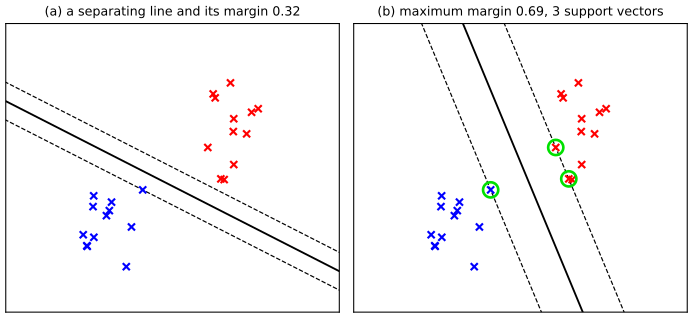
fig7_1() · in the notes · PDF · SVG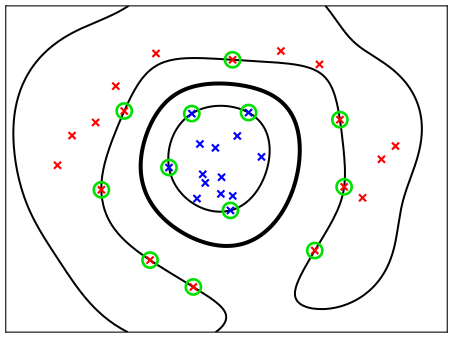
fig7_2() · in the notes · PDF · SVG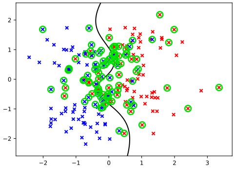
fig7_4() · in the notes · PDF · SVG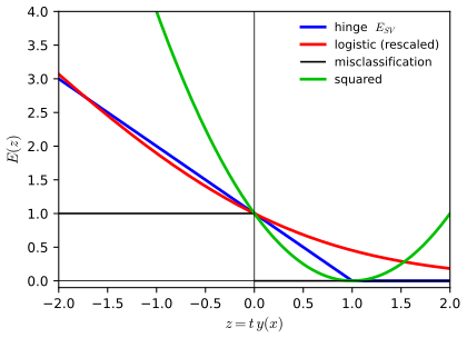
fig7_5() · in the notes · PDF · SVG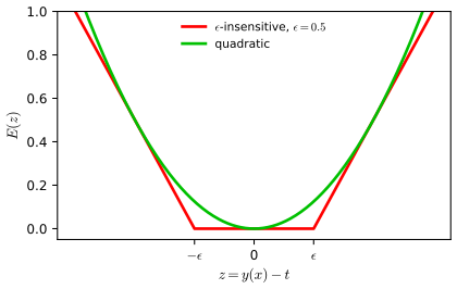
fig7_6() · in the notes · PDF · SVG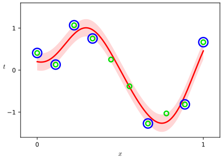
fig7_8() · in the notes · PDF · SVG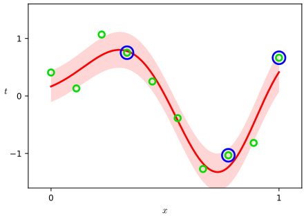
fig7_9() · in the notes · PDF · SVG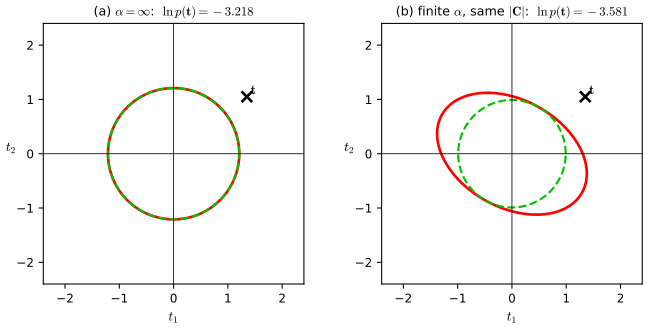
fig7_10() · in the notes · PDF · SVG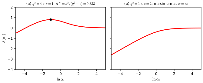
fig7_11() · in the notes · PDF · SVG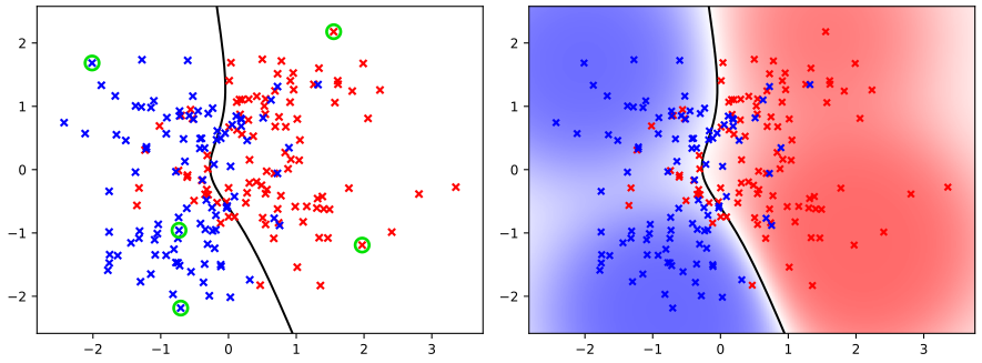
fig7_12() · in the notes · PDF · SVGChapter 8: Graphical Models
Source: ch08_graphical_models.py · run python3 ch08_graphical_models.py --list to list its figures · lecture notes: ch08-graphical-models.html
Module notes: data, settings and differences from the book
Bishop (2006), Chapter 8: Graphical Models.
Reproduces the figures of Chapter 8 of C. M. Bishop, Pattern Recognition and Machine Learning (Springer, 2006), pp. 359-422, written from scratch with numpy, scipy and matplotlib. Most figures of this chapter are diagrams; we draw them with the small helper class Diagram below and, wherever a diagram makes a numerical claim, compute the numbers with the algorithms of this file and print them on the figure. Every algorithm is a short function meant to be read next to the lecture notes (ch08-graphical-models.html):
* Section 8.1, Bayesian networks with discrete variables: joint_table (the factorisation (8.5)), ancestral_sample (Section 8.1.2), random_cpts; linear-Gaussian models: linear_gaussian_moments (the recursions (8.15) and (8.16)) and linear_gaussian_sample (8.14). * Section 8.2, conditional independence: cond_mutual_info (a numerical test of a | b given c on a joint table), d_separated (the reachability or "Bayes-ball" rule of Section 8.2.2), trails (every path between two nodes, each with the node that blocks it and why), markov_blanket (Section 8.2.2, Figure 8.26), fuel_gauge (the numbers (8.30) to (8.33)). * Section 8.3, Markov random fields: moralize (Section 8.3.4), ising_energy (8.42), icm (iterated conditional modes), gibbs_ising (Gibbs sampling at temperature 1, for the demo) and graph_cut_map (the exact MAP of (8.42) by a minimum s-t cut, Greig, Porteous and Seheult 1989), with make_binary_image (our own test image) and flip_noise. * Section 8.4, inference: chain_sum_product ((8.54) to (8.58)), FactorGraph with brute-force enumeration, sum_product ((8.61) to (8.72), observed variables by indicator functions as in Section 8.4.4), max_sum ((8.87) to (8.98) with back-tracking on a tree), chain_max_sum ((8.99) to (8.102), with the erratum: mu_{x_{n-1} -> f_{n-1,n}}(x_{n-1}) inside (8.101)), loopy_bp (the flooding schedule of Section 8.4.7).
Figures: 8.2, 8.6, 8.15 (with 8.16 to 8.20), 8.21, 8.22, 8.26, 8.28, 8.30, 8.32 (with 8.33), 8.40, 8.51, 8.52, 8.53. Run `python3 ch08_graphical_models.py --list`, or with no option for all figures (about ten seconds). Files go to ../img/ch08/ as PNG, SVG and PDF.
What differs from the book, and the choices made: * Figure 8.30: the book's image (hand-written "Bayes' Theorem") is not available. We render our own 150 x 200 binary image (the words "Graphical models" in a rounded box, drawn with matplotlib's DejaVu Sans Bold font; 21.2% of the pixels are ink), flip every pixel independently with probability 0.1 (numpy seed 8: 9.88% flipped), and use the book's beta = 1.0, eta = 2.1, h = 0. ICM visits the pixels in raster order, starting from x = y, until a whole sweep changes nothing (here the second sweep). Pixels that differ from the original: ICM 4.52% (book: 4%), graph cut 2.05% (book: 1%). Energies (8.42): noisy image -98150, ICM -104208, graph cut -105351 (the global minimum; the original image has -104821, so the exact MAP is not the original: the remaining 2% are corners and thin strokes that the Ising prior smooths away). The graph cut is checked against brute force on small images in checks_ch08.py. * Figures 8.15 to 8.22: the probabilities in the three 3-node graphs and in Figure 8.22 come from conditional probability tables drawn from a Dirichlet(1) distribution (numpy seed 3); the numbers written on the figures are conditional mutual informations, which are zero exactly when the independence holds. The fuel-gauge numbers are the book's: 0.315, 0.81, 0.257, 0.111. * Figure 8.52: binary variables with the integer factor tables FIG51_TABLES below, so that the messages are whole numbers; Figure 8.53: a chain of N = 5 variables with K = 3 states and the pairwise tables CHAIN_PSI below (the same chain as in the sum-product demo).
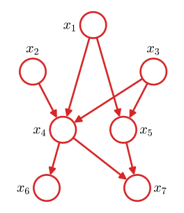
fig8_2() · in the notes · PDF · SVG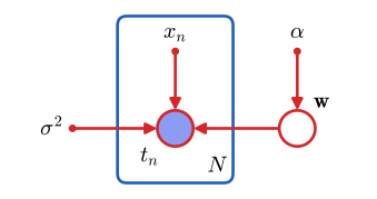
fig8_6() · in the notes · PDF · SVG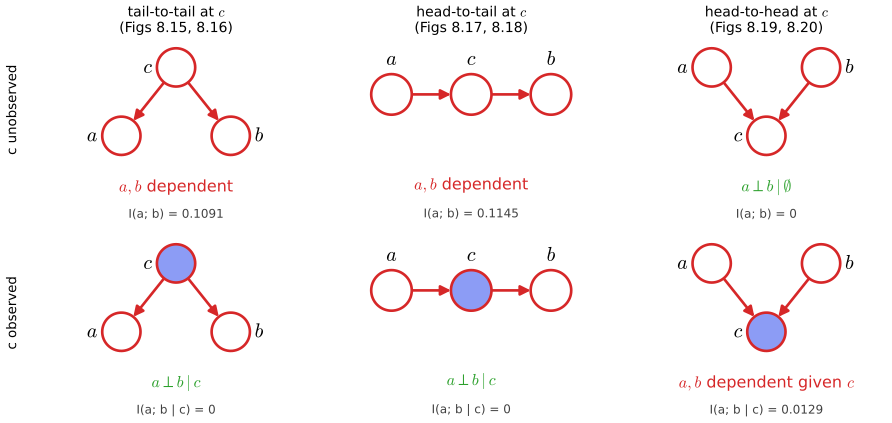
fig8_15() · in the notes · PDF · SVG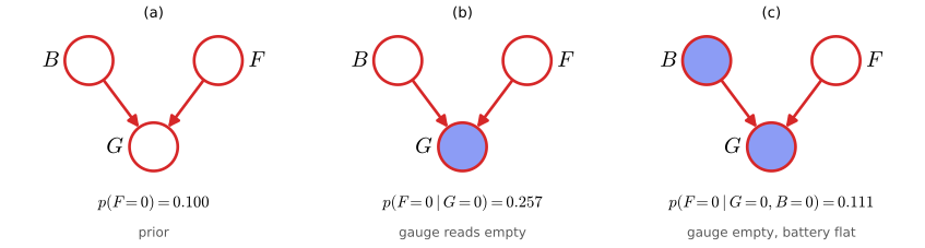
fig8_21() · in the notes · PDF · SVG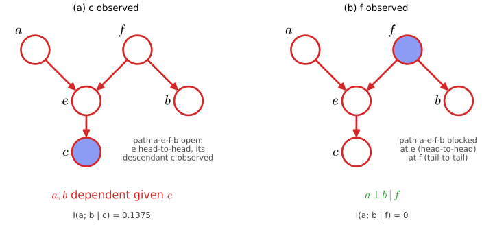
fig8_22() · in the notes · PDF · SVG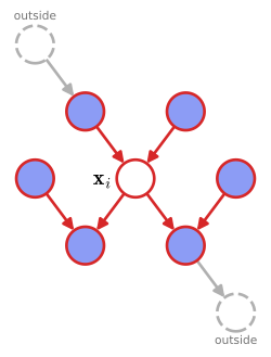
fig8_26() · in the notes · PDF · SVG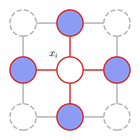
fig8_28() · in the notes · PDF · SVG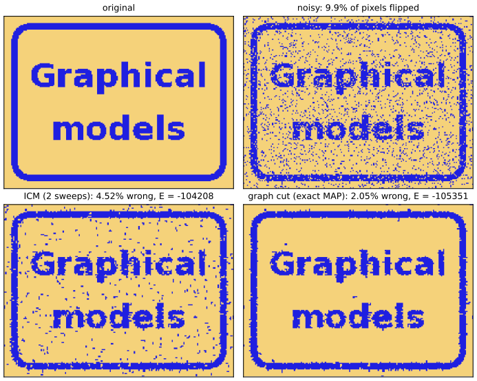
fig8_30() · in the notes · PDF · SVG
fig8_32() · in the notes · PDF · SVG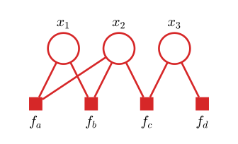
fig8_40() · in the notes · PDF · SVG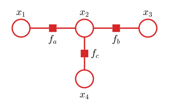
fig8_51() · in the notes · PDF · SVG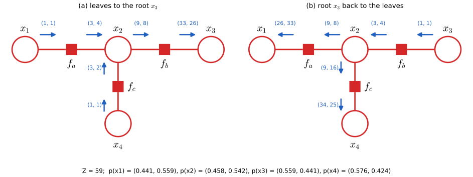
fig8_52() · in the notes · PDF · SVG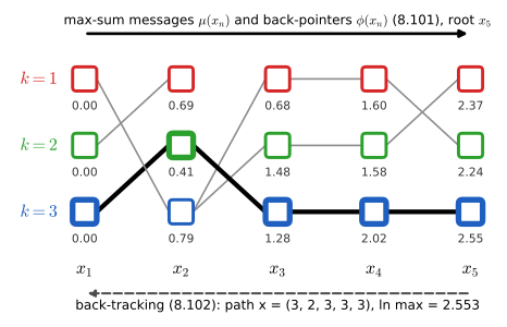
fig8_53() · in the notes · PDF · SVGChapter 9: Mixture Models and EM
Source: ch09_mixture_em.py · run python3 ch09_mixture_em.py --list to list its figures · lecture notes: ch09-mixture-models-em.html
Module notes: data, settings and differences from the book
Bishop (2006), Chapter 9: Mixture Models and EM.
Reproduces the numerical figures of Chapter 9 of C. M. Bishop, Pattern Recognition and Machine Learning (Springer, 2006), pp. 423-459, written from scratch with numpy and matplotlib. The algorithms are small functions meant to be read next to the lecture notes (ch09-mixture-models-em.html):
* K-means (Section 9.1): kmeans_e_step (9.2), kmeans_m_step (9.4), distortion (9.1), kmeans (the batch algorithm). * EM for Gaussian mixtures (Section 9.2.2): gmm_e_step (9.23), gmm_m_step (9.24)-(9.27), gmm_loglik (9.28), em_gmm. * EM for mixtures of Bernoulli distributions (Section 9.3.3): bernoulli_e_step (9.56), bernoulli_m_step (9.57)-(9.60), bernoulli_mixture_em. * The lower bound L(q, theta) (9.71) and KL(q||p) (9.72) of Section 9.4 for a mixture of two 1-D Gaussians with one free parameter (the mix1d_* functions), used for Figure 9.14 and by the demo em-bound-demo.html.
Figures: 9.1, 9.2, 9.3, 9.5, 9.7, 9.8, 9.10, 9.14. Run `python3 ch09_mixture_em.py --list`, `python3 ch09_mixture_em.py` (all figures, under a minute) or `python3 ch09_mixture_em.py --fig 9.1 9.8`. The PNGs are written to ../img/ch09/.
What differs from the book, and the choices made: * Figures 9.1, 9.2 and 9.8: the book does not print its starting values; we read them off Figure 9.1(a) and Figure 9.8(a): centres (1.4, -1.0) (red) and (-1.4, 1.0) (blue), and, for EM, covariances 0.6 I (the circles in Figure 9.8(a) have radius 0.77) and pi_k = 1/2. With this start every panel matches the book's: J after the first E step is 1048.4 (Figure 9.2 shows about 1050), and the fourth E step still moves one point from blue to red, as in the book's panel (h); the fifth E step changes nothing. EM reaches ln p(X) = -385.46 (standardised data) and is within 1e-8 of its limit by L = 20. * Figure 9.3: the book's photographs are not available; we use two public-domain photographs (Grace Hopper, U.S. Navy; astronaut Eileen Collins, NASA), averaged over 3 x 3 pixel blocks (200 x 170 and 170 x 170 pixels; the book's image has 240 x 180). K-means starts from K randomly chosen pixels (seeded; 3 starts, the lowest J kept) and runs until no assignment changes. * Figure 9.5: the mixture of Figure 2.23 is not tabulated in the book. Fitting ellipses to the contours of Figure 2.23(a) gives pi = (0.5, 0.3, 0.2), means (0.2, 0.4), (0.5, 0.5), (0.8, 0.6) and covariances 0.016 [[1, r], [r, 1]] with r = 0.75 for the red and blue components and r = -0.75 for the green one; we sample 500 points from it. * Figure 9.7: the book's picture is a sketch. We compute it for seven points: the broad component is the single-Gaussian fit to all seven points, the narrow one sits on the right-most point with sd 0.15, and the weights are 6/7 and 1/7. Panel (b), which is not in the book, shows ln p(X) as the narrow sd shrinks (it grows without bound), against a single Gaussian collapsing onto the same point (it falls without bound; compare Figure 1.14). * Figure 9.10: MNIST training images (the first 200 of each of the digits 2, 3 and 4), binarised at 0.5. EM is initialised exactly as the book describes (pi_k = 1/3; mu_ki uniform on (0.25, 0.75), then normalised so that sum_i mu_ki = 1) and run for 10 iterations. Logs of mu are taken after clipping to [1e-10, 1 - 1e-10], because some border pixels are never on. With this initialisation 10 iterations do not always separate the three digits (local maxima); with our seed 526 of the 600 images land in the component of their own digit. * Figure 9.14: the book's curves are schematic. We compute them for a real model: 40 points (the "two clusters" data of em-bound-demo.html) and the mixture 0.5 N(x|0, 2^2) + 0.5 N(x|theta, 0.6^2) whose only free parameter theta is the second mean; theta_old = 0. ln p(X|theta) is then not concave (a second, lower maximum near theta = -2.1), the bound at theta_old touches it with the same slope, and one M step moves theta from 0 to 0.712.
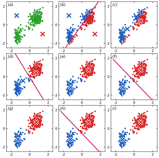
fig9_1() · in the notes · PDF · SVG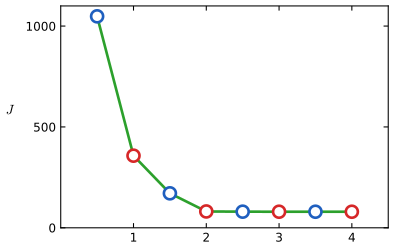
fig9_2() · in the notes · PDF · SVG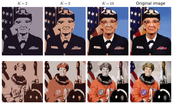
fig9_3() · in the notes · PDF · SVG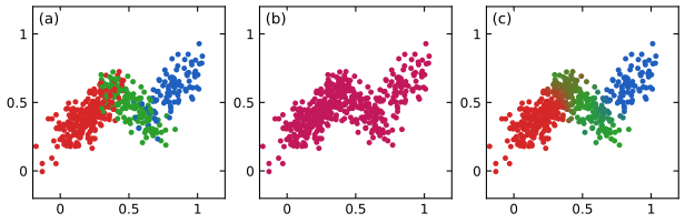
fig9_5() · in the notes · PDF · SVG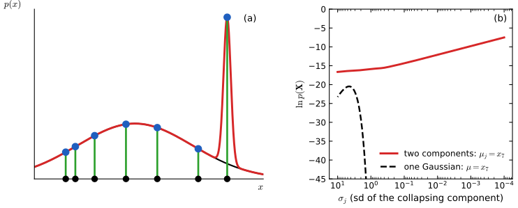
fig9_7() · in the notes · PDF · SVG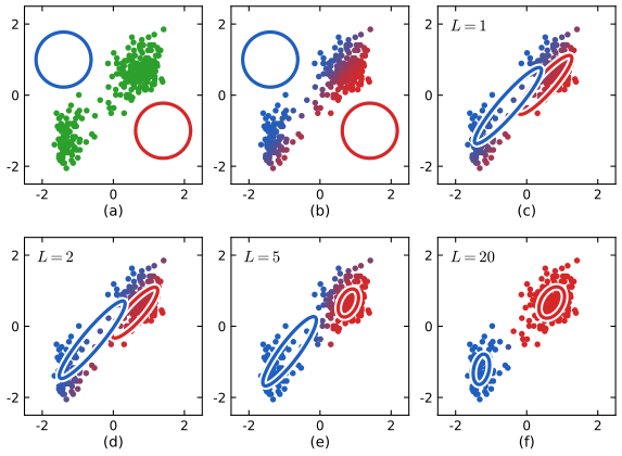
fig9_8() · in the notes · PDF · SVG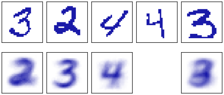
fig9_10() · in the notes · PDF · SVG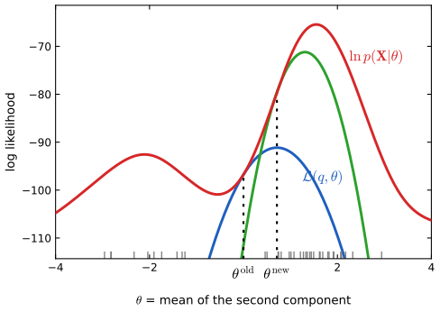
fig9_14() · in the notes · PDF · SVGChapter 10, Sections 10.1–10.4: Variational inference
Source: ch10_variational_inference.py · run python3 ch10_variational_inference.py --list to list its figures · lecture notes: ch10-approximate-inference.html
Module notes: data, settings and differences from the book
Bishop (2006), Chapter 10, Sections 10.1 to 10.4: variational inference.
Reproduces the numerical figures 10.1, 10.2, 10.3, 10.4, 10.6, 10.7 and 10.9 of C. M. Bishop, Pattern Recognition and Machine Learning (Springer, 2006), pages 461 to 491. One function per figure; run
python3 ch10_variational_inference.py --list python3 ch10_variational_inference.py --fig 10.6 10.7
The algorithms are small functions whose docstrings cite the book's equations, so that they can be read next to the lecture notes (ch10-approximate-inference.html):
skewed_log_density, laplace_1d, gauss_kl_qp_1d, moments_1d Section 10.1, Figure 10.1 mean_field_gaussian, factorised_kl_pq Section 10.1.2, Figure 10.2 mixture_log_density, gauss_kl_qp_2d, moment_match_mixture Section 10.1.2, Figure 10.3 normal_gamma_posterior, vb_gaussian, vb_gaussian_bound Section 10.1.3, Figure 10.4 vbgmm_init, vbgmm_e_step, vbgmm_m_step, vbgmm_bound, vb_gmm, vbgmm_predictive Section 10.2, Figures 10.6, 10.7 vb_linear_regression, vblr_bound Section 10.3, Figure 10.9
Corrections to the first printing used here (Svensen and Bishop's errata, and our own derivation): * (10.63) is nu_k = nu_0 + N_k. The first printing has nu_0 + N_k + 1, which is not the maximiser of the bound (the solution of Exercise 10.13 gives nu_0 + N_k); checks_ch10a.py confirms by finite differences that nu_0 + N_k is the stationary point. * (10.69): E[pi_k] = (alpha_0 + N_k) / (K alpha_0 + N) (alpha_0 in the numerator). * (10.110): the last term is ln Gamma(a_0), not ln Gamma(a_N). * (10.29) has (N + 1)/2, and (10.31) and (10.33) read 1/E[tau] = N/(N + 1) (mean(x^2) - 2 xbar E[mu] + E[mu^2]) and 1/E[tau] = mean(x^2) - xbar^2.
What the book does not specify, and the choices made here: * Fig 10.1: our Laplace approximation uses the exact second derivative at the mode z0 = 0.0775 (precision A = 2.546, sd 0.627, peak 0.636). The red curve of the book (here and in Fig 4.14) is narrower (sd about 0.52, peak 0.76), apparently a less accurate Hessian. The variational Gaussian (mean 0.707, sd 0.494) agrees with the book's green curve. * Fig 10.2: p has mean (0.5, 0.5), standard deviations 0.15 and correlation 0.95 (read off the book's 3-sd contours). * Fig 10.3: the bimodal p is our own equal mixture of two tilted Gaussians placed as in the book; contour levels are fractions of each density's maximum. * Fig 10.4: the book's data and prior are not given. We use N = 15 values drawn from N(0, 1) (numpy seed below, rounded to 3 decimals; the demo uses the same numbers), the prior mu_0 = 0, lambda_0 = 1, a_0 = b_0 = 1, and an initial guess placed as in panel (a). Contours are drawn at the same fractions of each density's maximum. * Figs 10.6 and 10.7: the book gives alpha_0 = 1e-3 and (typically) m_0 = 0. We take beta_0 = 1, W_0 = I and nu_0 = D = 2 on the standardised data. Starting point: unit Gaussian bumps on K data points chosen at random (a seeded K-means-like soft start), then one M step ('iteration 0'). The six starting rows of Fig 10.6 are fixed below and are also used by the demo vb-gmm-demo.html. * Fig 10.7: 100 random starts for each K = 1, ..., 6, with the ln K! term added as in the book, which does not say which alpha_0 it used. With alpha_0 = 1e-3 (or even 1) surplus components switch off, every K >= 2 reaches the same two-component fit and ln K! would then reward large K for nothing (it counts the K! relabellings of K distinct components in use). We use alpha_0 = 10, for which every component stays in use (as the book notes for Fig 10.6), so the correction applies; the bound then peaks at K = 2 as in the book. In our runs every start reached the same bound for each K (the book shows a few poorer local maxima), and K = 1 lies much further below than in the book's picture. * Fig 10.9: the cubic, the inputs (uniform on (-5, 5)) and the noise draw are ours; beta = 1/0.09 is known; with a_0 = b_0 = 0 the improper prior's normalising constant (the same for every degree) is omitted, so only differences between degrees matter.
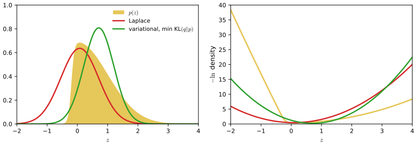
fig10_1() · in the notes · PDF · SVG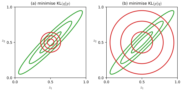
fig10_2() · in the notes · PDF · SVG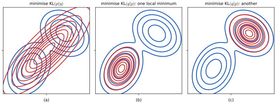
fig10_3() · in the notes · PDF · SVG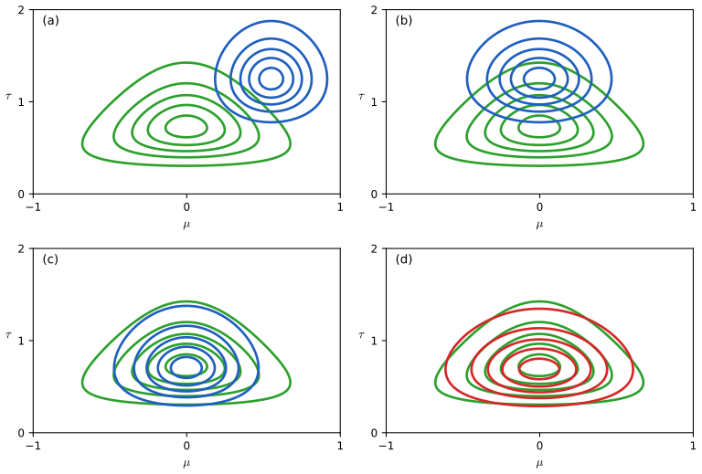
fig10_4() · in the notes · PDF · SVG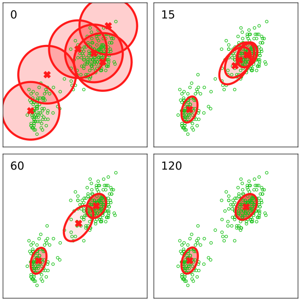
fig10_6() · in the notes · PDF · SVG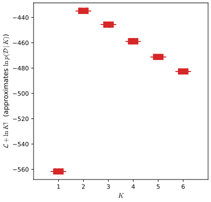
fig10_7() · in the notes · PDF · SVG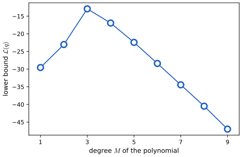
fig10_9() · in the notes · PDF · SVGChapter 10, Sections 10.5–10.7: Local variational methods and expectation propagation
Source: ch10_local_variational_ep.py · run python3 ch10_local_variational_ep.py --list to list its figures · lecture notes: ch10-approximate-inference.html
Module notes: data, settings and differences from the book
Bishop (2006), Chapter 10, Sections 10.5 to 10.7: local variational methods, variational logistic regression and expectation propagation (EP).
One function per figure; run `python3 ch10_local_variational_ep.py --list`. The figures are written to ../img/ch10/fig10-10.png ... fig10-17.png.
Algorithms, each with the book's equation numbers in its docstring:
Section 10.5 conjugate_exp_neg, tangent_exp_neg, binary_entropy, sigmoid_upper_bound, jj_lambda, sigmoid_lower_bound Section 10.6 vlr_e_step, vlr_m_step, vlr_bound, variational_logistic_regression (EM for xi, fixed prior), variational_logistic_regression_alpha (alpha inferred too), predictive_probability Figure 10.14 laplace_toy, kl_qp_gaussian_toy, ep_toy Section 10.7.1 ep_site_update, ep_clutter (every update (10.212) to (10.224), evidence included), vb_clutter, laplace_clutter, exact_clutter
Data. The figures and the two browser demos (variational-logistic-demo.html, ep-clutter-demo.html) draw their data from the same seeded generator: DemoRNG below is a line-by-line port of DK.rng in ../../demo-kit.js (mulberry32 uniforms and Box-Muller normals), so a seed gives the same data set in Python and in the browser.
What could not be reproduced exactly, and the choices made:
* Figure 10.10 and 10.12 are exact (they are plots of formulas). Figure 10.11 is a schematic in the book; we draw it for the convex function f(x) = 6.03 exp(-1.358 x) - 0.9 and slope eta = -0.43. * Figure 10.13: the book gives neither the data nor the prior. We draw 25 + 25 points, class t = 0 (crosses) with x1 ~ N(-1.1, 0.25^2), x2 ~ N(0.8, 1) and class t = 1 (circles) with x1 ~ N(1.1, 0.25^2), x2 ~ N(-1, 1), using seed LOGIT_SEED, which was picked among seeds giving a nearly vertical boundary like the book's. The model has a bias, phi(x) = (1, x1, x2) (the book's five sampled boundaries do not share a common point, so it has one too), and the prior is N(w | 0, alpha^-1 I) with alpha = LOGIT_ALPHA = 0.03, which gives contours like the book's. Inferring alpha as in Section 10.6.3 (a0 = b0 = 0.01) gives E[alpha] = 0.11 on these data. EM for xi starts from xi_n = 1 and needs a few hundred iterations here: with separable data the weights keep growing until the prior stops them. The predictive contours use the probit approximation (4.155) of Section 4.5.2, as the book says. * Figure 10.14 needs no data. The EP approximation of a density with one non-Gaussian factor converges after one update to the Gaussian with the mean and variance of p (moment matching). The variational (KL(q||p)) and EP curves agree with the book's; the book's Laplace curve is narrower (peak about 0.76) than the Laplace approximation itself, whose mode is z0 = 0.0775 with precision -d2 ln p(z0) = 2.54 (peak 0.64), as in our Figure 10.1. * EP is not guaranteed to converge to a good solution (Section 10.7). On some clutter data sets (for example seeds 6 and 23 with N = 20) the first sweep is captured by two far-out clutter points and EP settles at a poor fixed point; its evidence estimate is then far below the exact one, which reveals the failure. The seeds used here do not do this. * Figure 10.15: N = 20 points, theta = 3, w = 0.5, a = 10 (seed CLUTTER_SEED). * Figure 10.16: the book shows two unspecified examples. We take x_n = 2 and the cavity distributions N(theta | 0, 0.3^2) (left) and N(theta | 3, 0.3^2) (right), which is what the book's panels show, and compute f~_n by the EP update (10.216) to (10.222). * Figure 10.17: N = 200 points, theta = 3 (seed CLUTTER_SEED), D = 1. Minka (2001), whose experiment the book reproduces, counted flops with MATLAB. We count them explicitly with the convention stated next to FLOP_CONVENTION below, so our absolute numbers differ from the book's, but the comparison between the methods is like for like. The book plots the absolute error of the evidence p(D) (about 10^-200 here); we plot the error of ln p(D), which is the relative error of p(D) for small errors and is easier to read.
Errata applied (Bishop's PRML errata list, pages 493 to 513): * eta replaces lambda in Section 10.5 up to (10.141); (10.141) to (10.143) and (10.164) in their corrected forms; (10.177) with a_N, b_N; (10.183) with E[w w^T] = Sigma_N + mu_N mu_N^T; the left-hand sides of (10.217), (10.218) are m^new and v^new. * Two further inconsistencies, not in the errata list, are handled here and checked numerically in checks_ch10b.py: (i) (10.222) is the coefficient of the unnormalised site f~_n(theta) = s_n exp(-||theta - m_n||^2 / (2 v_n)) used by Minka (2001), not of s_n N(theta | m_n, v_n I) as written in (10.213); in the notation of (10.213) the coefficient is s_n = Z_n / N(m_n | m^\n, (v_n + v^\n) I). (ii) (10.223) and (10.224) must include the prior factor f~_0 = p(theta), that is the product and the sum start at n = 0; otherwise the prior's normalisation (2 pi b)^(-D/2) is lost. With the sites in Minka's form the evidence is ln p(D) ~ (D/2) ln(2 pi v) + B/2 - (D/2) ln(2 pi b) + sum_n ln s_n, which is exact when w = 0 (a conjugate Gaussian model).
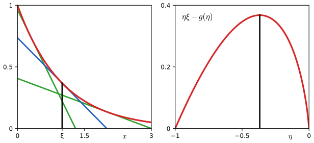
fig10_10() · in the notes · PDF · SVG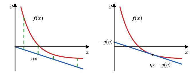
fig10_11() · in the notes · PDF · SVG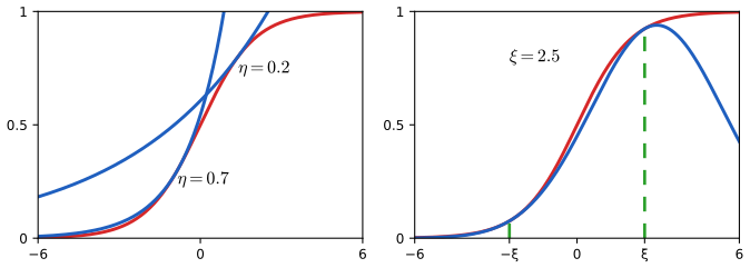
fig10_12() · in the notes · PDF · SVG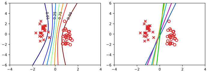
fig10_13() · in the notes · PDF · SVG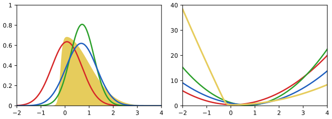
fig10_14() · in the notes · PDF · SVG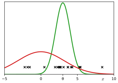
fig10_15() · in the notes · PDF · SVG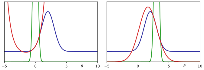
fig10_16() · in the notes · PDF · SVG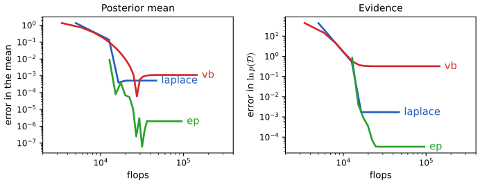
fig10_17() · in the notes · PDF · SVGChapter 11: Sampling Methods
Source: ch11_sampling.py · run python3 ch11_sampling.py --list to list its figures · lecture notes: ch11-sampling-methods.html
Module notes: data, settings and differences from the book
Bishop (2006), Chapter 11: Sampling Methods.
Reproduces the numerical figures of Chapter 11 of C. M. Bishop, Pattern Recognition and Machine Learning (Springer, 2006), pp. 523-558, written from scratch with numpy, scipy and matplotlib. Every sampler is a small function meant to be read next to the lecture notes (ch11-sampling-methods.html):
* Section 11.1.1, transformations of uniform numbers: inverse_cdf (11.5)-(11.6), exponential_from_uniform (11.7), cauchy_from_uniform (11.8, Exercises 11.3 and 11.7), box_muller (11.10)-(11.12, polar form, with the erratum ln r^2), gaussian_cholesky (Exercise 11.5). * Section 11.1.2, rejection sampling: rejection_sample (11.13)-(11.14), with the gamma density (11.15) and the scaled Cauchy envelope (11.16) in gamma_cauchy_envelope. * Section 11.1.3, adaptive rejection sampling (Gilks and Wild 1992): ars_hull builds the piecewise exponential envelope (11.17) from tangent lines, adaptive_rejection_sample draws from it (Exercises 11.8 and 11.9). * Sections 11.1.4 and 11.1.5: importance_sampling (11.19)-(11.23) with the effective sample size, sir (sampling-importance-resampling, (11.25)-(11.27)). * Section 11.2: metropolis (11.33), metropolis_hastings (11.44), mh_transition_matrix (the kernel on a finite space, for the detailed-balance check (11.40), (11.45)), random_walk_second_moment ((11.34)-(11.36), Exercise 11.10). * Section 11.3: gibbs_gaussian (11.46)-(11.48), overrelaxed_gibbs (Adler's over-relaxation (11.50)), ordered_overrelaxed_gibbs (Neal 1999). * Section 11.4: slice_sample (11.51)-(11.52), with stepping out and shrinking (Neal 2003). * Section 11.5: leapfrog (11.64)-(11.66), hamiltonian (11.57), hmc (hybrid Monte Carlo, acceptance (11.67), random direction of integration). * Section 11.6: partition_ratio (11.72, with the erratum: the factor 1/L) and chained_partition_ratio (11.74)-(11.75). * Diagnostics: autocorrelation, integrated_autocorr_time, effective_sample_size. * JSRandom: the seeded generator of the browser demos (DK.rng in courses/demo-kit.js: mulberry32 uniforms and Box-Muller normals). Passing JSRandom(seed) instead of a numpy Generator makes metropolis, gibbs_gaussian, slice_sample, hmc, ... use exactly the numbers of the demos, which is how the demos are cross-checked against this file.
Figures: 11.2 to 11.14. Run `python3 ch11_sampling.py --list`, `python3 ch11_sampling.py` (all figures, about a minute) or `python3 ch11_sampling.py --fig 11.9 11.13`. The PNGs are written to ../img/ch11/.
What differs from the book, and the settings chosen where the book gives none: * The book's Figures 11.2, 11.3, 11.4, 11.6, 11.8, 11.10, 11.11, 11.13 and 11.14 are sketches. We compute each of them from a real sampler and add panels with the numbers behind the sketch. The bimodal density used in Figures 11.2, 11.4, 11.8 and 11.13 (and in the demos) is p(z) = 0.55 N(z|-2, 0.75^2) + 0.45 N(z|2, 0.95^2); its unnormalised version p_tilde drops the factors 1/(sqrt(2 pi) s_k), so Z_p = sqrt(2 pi) (0.55 x 0.75 + 0.45 x 0.95) = 2.1055. * Figure 11.4: proposal q(z) = N(z|0, 2.2^2), k the smallest constant with k q >= p_tilde (found numerically): k = 4.841, so the acceptance (1/k) int p_tilde (11.14) is 0.435. * Figure 11.5: the curves are Gam(z|10, 1) (peak 0.132 at z = 9, as in the book) and the Cauchy envelope with c = a - 1 = 9, b^2 = 2a - 1 = 19 and the smallest k; we find k = 1.804, so the acceptance rate is 1/k = 0.554. * Figure 11.6: target Gam(z|10, 1) again (log-concave); starting abscissae 4, 8.5, 14, whose envelope accepts with probability 0.863. Following the book, a point is added to the envelope only when it is rejected (Gilks and Wild also use a lower squeeze function; we do not, to keep the code short). * Figure 11.7: sigma_p = 1, sigma_q = 1.1 (read off the figure); the right panel adds the acceptance (sigma_p/sigma_q)^D against D (1/20959 for sigma_q/sigma_p = 1.01, D = 1000, the book's "1/20,000"). Its Monte Carlo points use the fact that the acceptance probability p(z)/(k q(z)) depends on z only through |z|^2, which under q is sigma_q^2 times a chi-squared variable with D degrees of freedom; this is exactly equivalent to drawing the D coordinates and is much cheaper for D = 1000. * Figure 11.8: q(z) = N(z|0, 2^2), f(z) = tanh(0.6 (z + 1)); a badly placed q = N(2, 0.8^2) for comparison. * Figure 11.9: the book gives the proposal sd (0.2) and the number of candidates (150) but not the target. The ellipse in the figure has centre (1.5, 1.5), marginal sd 1.06 and correlation 0.76 if read as a one-sd contour, as the caption says. With that target a proposal sd of 0.2 is rejected only about 20 times in 150, and the chain would leave the ellipse most of the time; read as the two-sd contour, the target (covariance [[0.28, 0.2125], [0.2125, 0.28]], principal sds 0.70 and 0.26) gives about 40 rejections in 150 and a chain that stays mostly inside, as in the book. We use the second reading, draw both contours, start at (1.0, 1.0) and use numpy seed 16, which gives 43 rejections as in the book. * Figures 11.10 and 11.12: random-walk Metropolis with proposal sd rho = sigma_min on Gaussians with sigma_max / sigma_min = 2, 4, 8, 16 and 32 (integrated autocorrelation time by Sokal's automatic window, c = 5, 16 chains), and Gibbs sampling with correlation 0.5 ... 0.995 (exact IAT from the linear sweep map, measured IAT by batch means over 100 chains). File fig11-12 is our companion to the book's Figure 11.11 (the book's Figure 11.12 is a graphical-model sketch of Markov blankets, not a numerical figure). * Figure 11.13: w = 0.5 for the stepping-out panel, numpy seed 0 (four steps out, three candidates rejected before one is accepted). * Figure 11.14: panels (a) and (b) shear a rectangle of phase space with the potential E(z) = 1 - cos(2 z) and eps = 0.6 (the book's sketch has no numbers); panels (c) and (d) use the standard Gaussian E(z) = z^2 / 2.
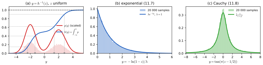
fig11_2() · in the notes · PDF · SVG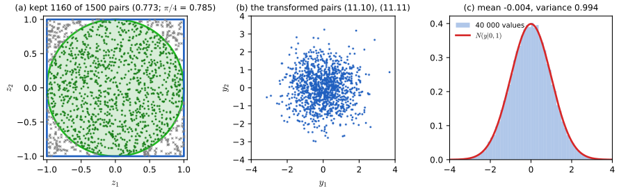
fig11_3() · in the notes · PDF · SVG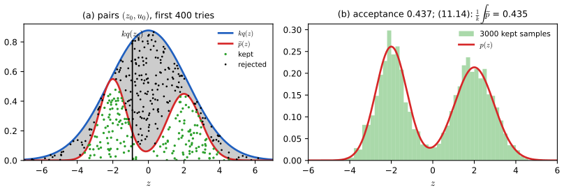
fig11_4() · in the notes · PDF · SVG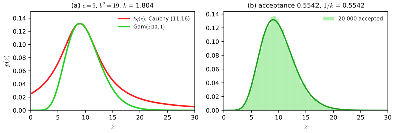
fig11_5() · in the notes · PDF · SVG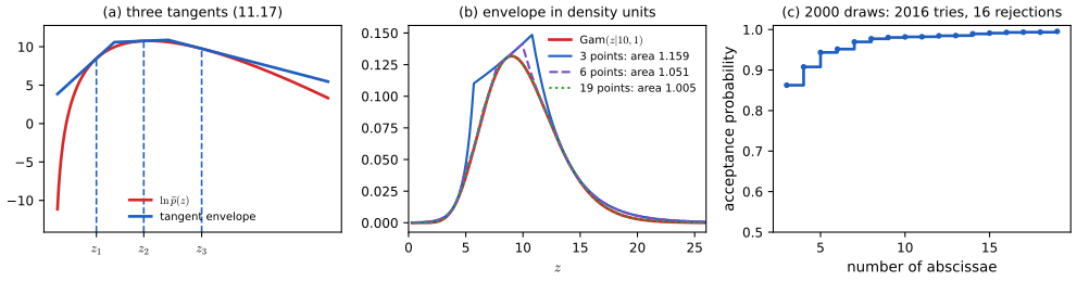
fig11_6() · in the notes · PDF · SVG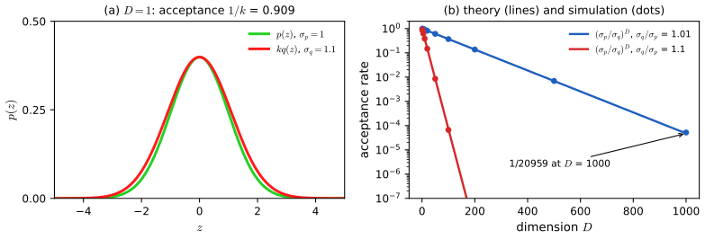
fig11_7() · in the notes · PDF · SVG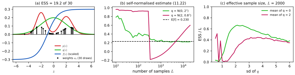
fig11_8() · in the notes · PDF · SVG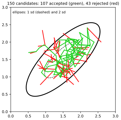
fig11_9() · in the notes · PDF · SVG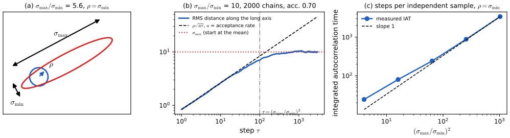
fig11_10() · in the notes · PDF · SVG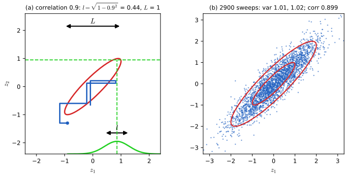
fig11_11() · in the notes · PDF · SVG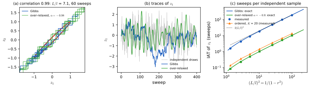
fig11_12() · in the notes · PDF · SVG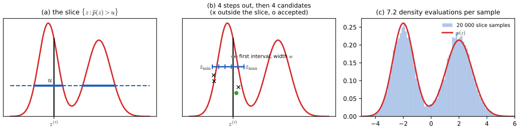
fig11_13() · in the notes · PDF · SVG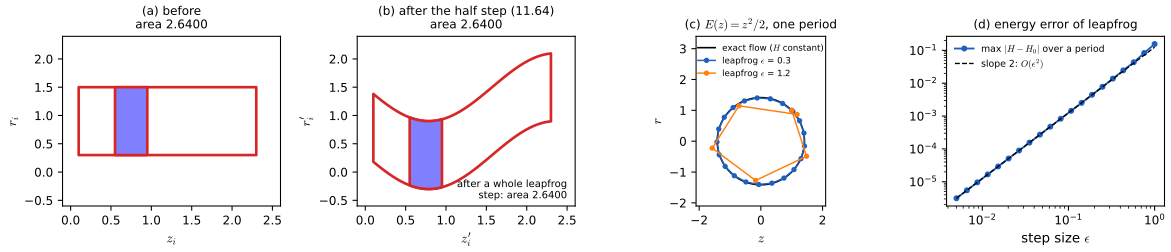
fig11_14() · in the notes · PDF · SVGChapter 12: Continuous Latent Variables
Source: ch12_continuous_latent.py · run python3 ch12_continuous_latent.py --list to list its figures · lecture notes: ch12-continuous-latent-variables.html
Module notes: data, settings and differences from the book
Bishop (2006), Chapter 12: Continuous latent variables.
One function per figure; run `python3 ch12_continuous_latent.py --list` to see them, `python3 ch12_continuous_latent.py --fig 12.12` to make one, or no option to make all.
Algorithms (small readable functions, each citing the book's equations): pca, pca_small_n, pca_reconstruct, whiten Section 12.1, (12.1)-(12.30) fisher_direction Section 4.1.4, (4.30), for Figure 12.7 ppca_ml, ppca_loglik, ppca_posterior Section 12.2.1, (12.36)-(12.48) ppca_em, ppca_em_missing Section 12.2.2, (12.54)-(12.57) em_pca (12.58), (12.59): the sigma^2 -> 0 limit bayesian_pca Section 12.2.3, ARD (12.62), (12.63) bayesian_pca_gibbs Gibbs sampler of Figure 12.15 factor_analysis_em, fa_loglik Section 12.2.4, (12.65)-(12.70) gaussian_kernel, kernel_pca, kernel_pca_project Section 12.3, (12.80)-(12.87) gtm_fit Section 12.4.3; Bishop, Svensen and Williams (1998)
What could not be reproduced exactly, and the choices made: * Figures 12.1, 12.3 to 12.5 use the MNIST test-set threes (1010 images, pixel values 0 to 255). The book's eigenvalues 3.4, 2.8, 2.4, 1.6 x 10^5 are reproduced to two figures, and the digit of Figures 12.1 and 12.5 is MNIST test image 44 (correlation 0.99999 with the book's picture). For Figure 12.1 the 28 x 28 digit is enlarged to 64 x 64 (bilinear) as in the text (p. 559) and placed in a 100 x 100 field with a random rotation (+-25 degrees) and shift (+-16 pixels). * Figure 12.2 and Figure 12.9 are drawn from small made-up configurations, but every line, point and contour is computed (the principal axis, the projections, the Gaussian contours). * Figure 12.6: the right-hand panel whitens the original data (12.24) (whitening the standardised data gives the same picture up to a rotation); as in the book's figure, the horizontal axis is the whitened coordinate along the minor principal axis and the vertical axis along the major one. * Figure 12.7: the two-class data are simulated (the book's are not available). * Figures 12.8, 12.11, 12.21: the oil flow training set (1000 points). Eigenvector signs are chosen to match the book's orientation. In 12.11 the PPCA model (M = 2) is fitted to the first 100 points; for the right panel 30% of the 1200 values are deleted at random (seeded, every point loses at least one value) and the exact EM for data missing at random is used. * Figure 12.12: the ten data points are read off the book's figure (then centred); the initial W points along (2, -1) as in panel (b). * Figure 12.14: 300 points in D = 10, standard deviation 1 along 3 random orthonormal directions and 0.5 along the other 7; M = 9. Maximum likelihood PPCA and Bayesian PCA are both run by EM from the same random start, so the ML solution comes with an arbitrary rotation R (12.45). * Figure 12.15: the book gives no settings. We use D = 4, M = 3, N = 50 points from a PPCA model with one direction of variance 0.7 plus isotropic noise variance 0.1, vague Gamma(0.001, 0.001) priors on the alpha_i and on 1/sigma^2, and mu fixed at the sample mean; 10,000 Gibbs sweeps. The barrier between the three modes grows with N: with N = 100 we saw no switch at all. * Figure 12.17: the toy data of Schoelkopf et al. (1998): three clusters of 30 points (sd 0.1) centred at (-0.5, -0.2), (0, 0.6), (0.5, 0), kernel exp(-|x - x'|^2/0.1) (12.86). The titles give the eigenvalues of the centred Gram matrix (12.85), which equal N lambda_i by (12.80). The points are our own draw, so the eigenvalues differ slightly from the book's. * Figure 12.21: GTM with a 20 x 20 latent grid on [-1, 1]^2, an 8 x 8 grid of Gaussian basis functions plus a bias, width equal to twice the spacing of the basis centres, weight regularisation alpha = 0.01, initialised from PCA and run for 200 EM iterations (the book does not give its settings; these gave the highest likelihood among the grids we tried).

fig12_1() · in the notes · PDF · SVG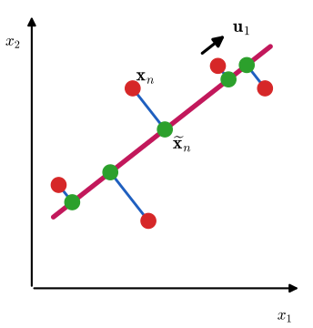
fig12_2() · in the notes · PDF · SVG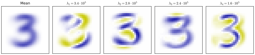
fig12_3() · in the notes · PDF · SVG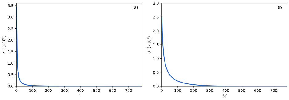
fig12_4() · in the notes · PDF · SVG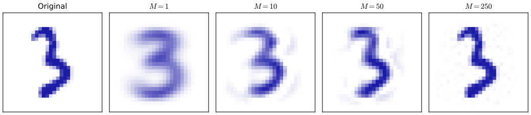
fig12_5() · in the notes · PDF · SVG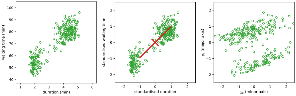
fig12_6() · in the notes · PDF · SVG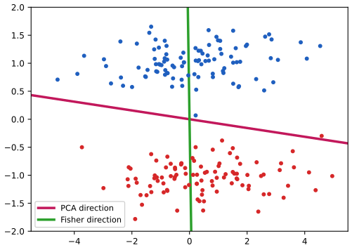
fig12_7() · in the notes · PDF · SVG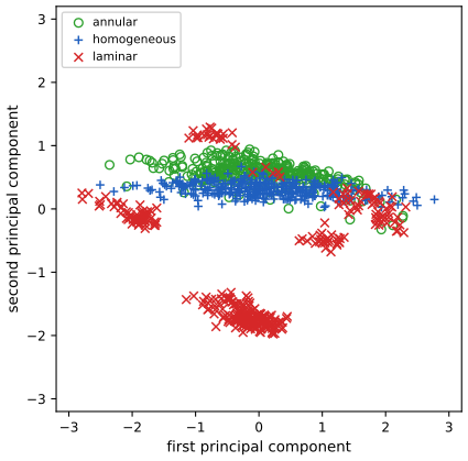
fig12_8() · in the notes · PDF · SVG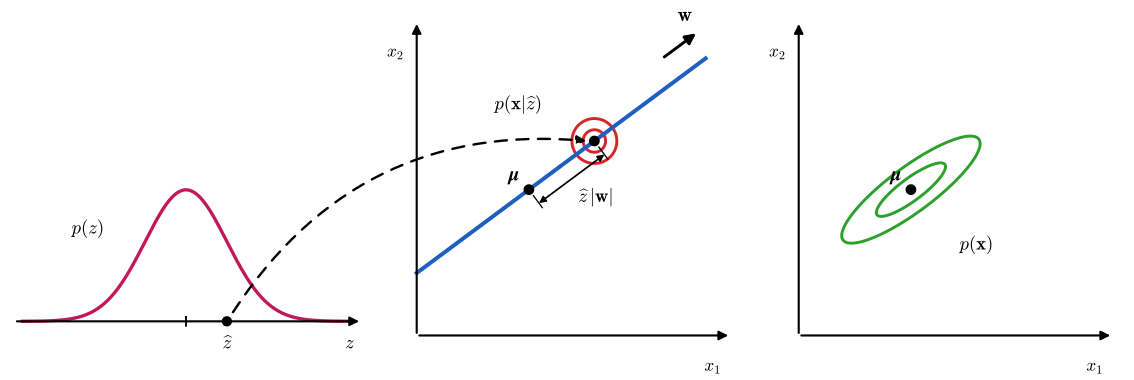
fig12_9() · in the notes · PDF · SVG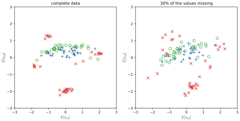
fig12_11() · in the notes · PDF · SVG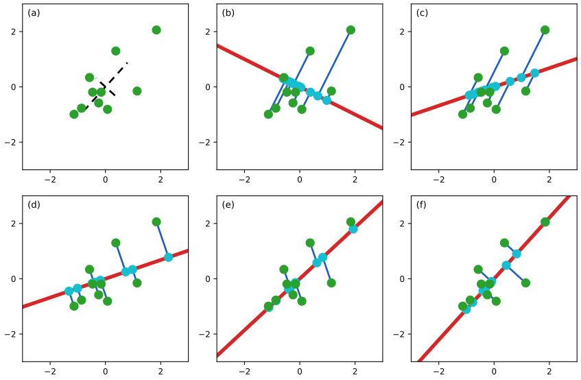
fig12_12() · in the notes · PDF · SVG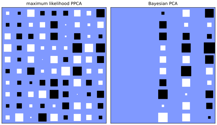
fig12_14() · in the notes · PDF · SVG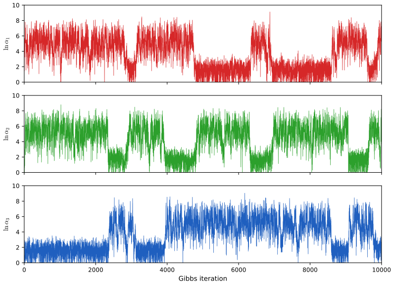
fig12_15() · in the notes · PDF · SVG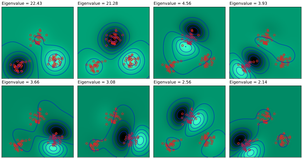
fig12_17() · in the notes · PDF · SVG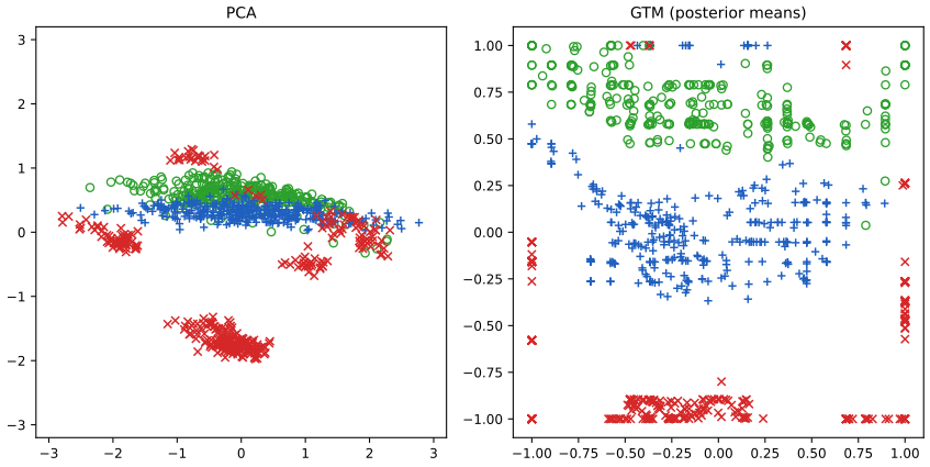
fig12_21() · in the notes · PDF · SVGChapter 13: Sequential Data
Source: ch13_sequential_data.py · run python3 ch13_sequential_data.py --list to list its figures · lecture notes: ch13-sequential-data.html
Module notes: data, settings and differences from the book
Bishop (2006), Chapter 13: Sequential Data.
Reproduces the numerical figures of Chapter 13 of C. M. Bishop, Pattern Recognition and Machine Learning (Springer, 2006), pp. 605-652, written from scratch with numpy, scipy and matplotlib. Every algorithm is a small function meant to be read next to the lecture notes (ch13-sequential-data.html):
* Section 13.2, hidden Markov models: hmm_sample (ancestral sampling, Section 13.2 and Figure 13.8), emission_logprob (Gaussian emissions (13.20)-(13.21) or a discrete table (13.22)), forward_backward_unscaled (the alpha-beta recursions (13.36)-(13.43)), forward_backward (the scaled recursions (13.59)-(13.65), with ln p(X) from (13.63)), viterbi (max-sum on the lattice, (13.68)-(13.71), with the errata to (13.68), (13.70), (13.71)), baum_welch (EM, E step (13.33)-(13.43), M step (13.18)-(13.23); several sequences; Gaussian or discrete emissions; a left-to-right model keeps its zero transitions). * Section 13.3, linear dynamical systems: lds_sample ((13.75)-(13.77)), kalman_filter ((13.88)-(13.97), with V0 renamed P0 as in the errata), rts_smoother ((13.100)-(13.104)), lds_em (E step (13.105)-(13.107), M step (13.110)-(13.116) with the errata to (13.106), (13.114) and (13.116)). * Section 13.3.4, particle_filter ((13.117)-(13.119): weights, mixture representation of the predictive distribution, resampling from that mixture). * JSRandom (imported from ch11_sampling.py): the seeded generator DK.rng of the browser demos. Passing JSRandom(seed) to hmm_sample, lds_sample, pf_simulate and particle_filter reproduces the demos' sequences and particles number for number.
Figures: 13.1, 13.8, 13.11, 13.12, 13.13, 13.16, 13.22, 13.23. Run `python3 ch13_sequential_data.py --list`, `python3 ch13_sequential_data.py` (all figures, under a minute) or `python3 ch13_sequential_data.py --fig 13.8 13.22`. Files go to ../img/ch13/.
What differs from the book, and the settings chosen where the book gives none: * Figure 13.1: the book's recording of the spoken words "Bayes' theorem" is not available. We synthesise a speech-like signal with a source-filter model (a glottal pulse train with a falling pitch, three formant resonators whose frequencies move through the vowels of "Bayes' theorem", and filtered noise for the fricatives z and th) and show its spectrogram. It is a SUBSTITUTE, labelled as such; it makes the book's point (successive spectra are strongly correlated), which a third panel quantifies. * Figure 13.8: the emission means and covariances are read off the book's contours: means (0.31, 0.72), (0.30, 0.20), (0.70, 0.47); standard deviations along the principal axes (0.10, 0.035) at +45 degrees, (0.085, 0.035) horizontal, (0.10, 0.04) at -45 degrees; contours at 2/3, 4/3 and 2 standard deviations. Transition matrix: 0.9 on the diagonal and 0.05 elsewhere, pi uniform, as in the caption. The 50 points use JSRandom(SEED_FIG8), so preset 1 of hmm-demo.html draws the same sequence. * Figure 13.11: the book's 45 on-line handwritten digits are not available. We SYNTHESISE 45 pen trajectories of a digit '2' (an arc, a cusp or small loop, and a base stroke, with random proportions, slant, size and jitter), turn each into line segments of fixed length whose angles are quantised to 16 values (as in the book), and fit a 16-state left-to-right HMM with a 16 x 16 emission table by 25 iterations of Baum-Welch. A left-to-right chain never leaves its last state, so to draw a sample we run the chain until it enters state 16 and then stay there for the average time the training sequences spend in that state (from the posterior gamma); every other step is sampled from the fitted model. * Figures 13.12, 13.13 and 13.16 are lattice diagrams in the book. We draw the same lattices for a small 3-state HMM with discrete emissions (LATTICE_* below) and write the actual values of alpha, beta and omega on the nodes. The example is chosen so that the Viterbi path differs from the sequence of individually most probable states. * Figure 13.22: the book's object and noise levels are not given. We use a constant-velocity model in the plane (state: position and velocity; white-noise acceleration with spectral density q = 0.05; position measurements with standard deviation 0.8), 12 time steps, and add a second panel with the Rauch-Tung-Striebel smoother. * Figure 13.23 is a sketch in the book. We compute it from a run of the particle filter with L = 12 particles on the univariate nonlinear growth model of Kitagawa (1996) and Gordon, Salmond and Smith (1993), whose observation x = z^2/20 + noise makes p(x|z) bimodal in z, as in the book's sketch; a second panel shows the whole run with L = 500 particles.
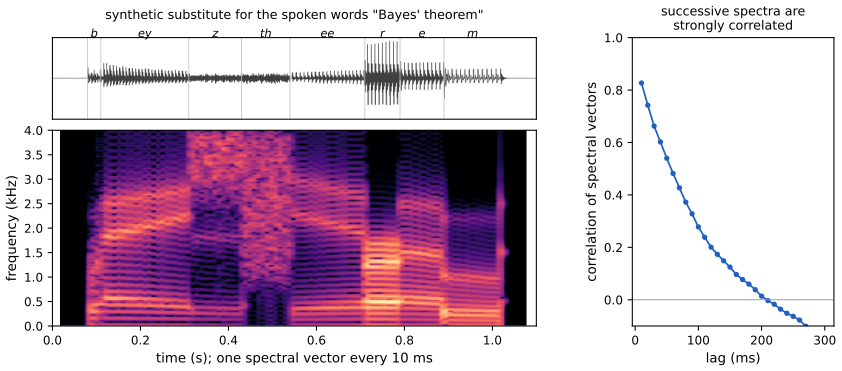
fig13_1() · in the notes · PDF · SVG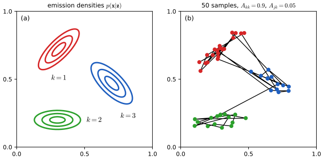
fig13_8() · in the notes · PDF · SVG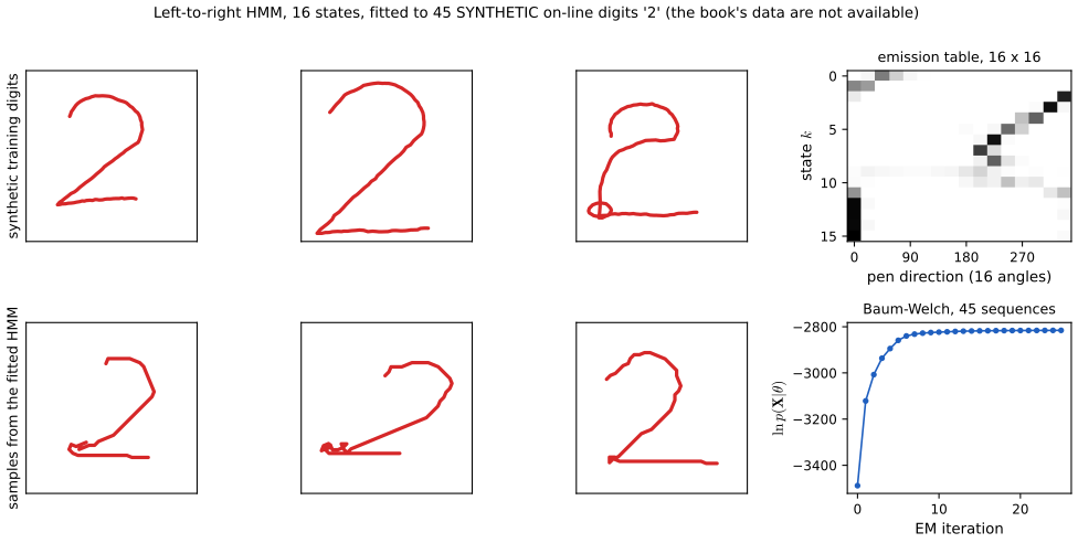
fig13_11() · in the notes · PDF · SVG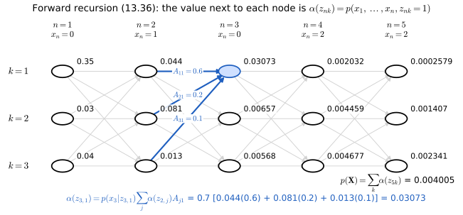
fig13_12() · in the notes · PDF · SVG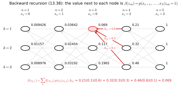
fig13_13() · in the notes · PDF · SVG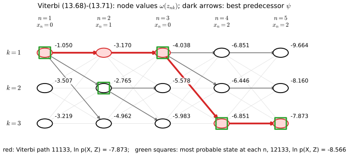
fig13_16() · in the notes · PDF · SVG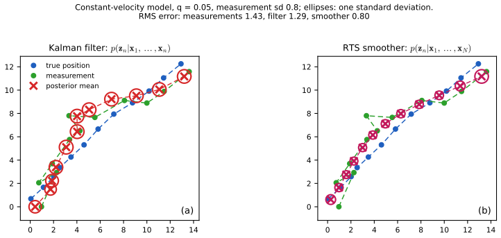
fig13_22() · in the notes · PDF · SVG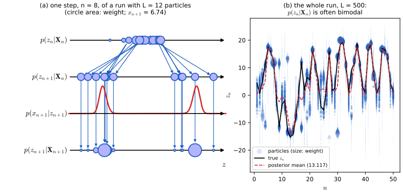
fig13_23() · in the notes · PDF · SVGChapter 14: Combining Models
Source: ch14_combining_models.py · run python3 ch14_combining_models.py --list to list its figures · lecture notes: ch14-combining-models.html
Module notes: data, settings and differences from the book
Bishop (2006), Chapter 14: Combining models.
One function per figure; run `python3 ch14_combining_models.py --list` to see them, `python3 ch14_combining_models.py --fig 14.2` to make one, or no option to make all.
Algorithms (small readable functions, each citing the book's equations): committee_errors Section 14.2, E_AV and E_COM, (14.7)-(14.11) fit_stump, adaboost, adaboost_f Section 14.3, AdaBoost with decision stumps, (14.15)-(14.21) exponential_error, ... (four losses) Section 14.3.2, the error functions of Figures 14.3, 14.4 grow_tree, prune_tree, pruning_path Section 14.4, CART trees and the pruning criterion (14.29)-(14.33) bagging, fit_polynomial Section 14.2, bootstrap committees (14.7) mixture_linear_regression_em Section 14.5.1, EM for a mixture of linear regressions, (14.34)-(14.44) irls_logistic, mixture_logistic_em Section 14.5.2, EM with IRLS in the M step, (14.45)-(14.52) mixture_of_experts_em Section 14.5.3, linear experts with a softmax gate, (14.53)
What could not be reproduced exactly, and the choices made: * Figure 14.2: the book uses 30 points of its two-class synthetic data (Appendix A, Figure A.7) but does not publish them. BOOST_X, BOOST_T below are those 30 points read off the book's figure (circle centres located in the image, accurate to about 0.005). The base learners are decision stumps with thresholds half-way between neighbouring data values; equal weighted errors are broken by taking the last best stump in the order (x1 before x2, increasing threshold, sign +1 before -1). With these points and this rule our stumps for m = 1, 2, 3, 6, 10 and 150 are exactly the book's dashed lines (x1 = 0.59, x1 = -0.007, x2 = -1.72, x2 = 0.087, x2 = -0.867, x1 = 0.417); the first-best rule swaps the first two stumps and then drifts away from the book. Circle radius is proportional to the weight w_n^(m) used to train the latest stump, scaled so that the largest circle has a fixed size (at m = 1 all weights are equal and the circles are drawn at half that size, as in the book). The ensemble boundary is drawn exactly, as the edges between the axis-aligned cells on which sign(f_m) is constant. * Figures 14.3 and 14.4 are exact (the cross-entropy is divided by ln 2 as in the text, p. 662). * Figures 14.5 and 14.6 are schematic in the book. Here the partition and the tree are drawn from one tree object (the Node class used by the CART code), with theta_1 = 0.4, theta_2 = 0.3, theta_3 = 0.7, theta_4 = 0.8 on the unit square, the proportions of the book's drawing. * Figures 14.8 and 14.9: the book's 20 points have x = linspace(-1, 1, 20) exactly; their targets t (TWO_LINES_T) and the two initial lines (MIX_W0) are read off the book's figure. The text says beta was initialised to the reciprocal of the variance of the targets; we use the variance with the N - 1 divisor, with which our state after 30 EM iterations matches the book's centre panel (the change near iteration 30 is so fast that the divisor N gives the same picture one iteration earlier). After 50 iterations the log likelihood is -3.08 (book: -3.0) and a single linear regression has -27.66 (book: -27.6). * Figure 14.10: the book's data are not available. We draw 100 points from each of four Gaussian clusters with standard deviation 0.5: class "red" around (-1.5, 0) and (1.5, 0), class "blue" around (0, 1.5) and (0, -1.5), which is what the book's figure shows. Panel (a) is shaded with the exact class probability of this generating model, which is sharper than the book's shading (the book's colours fit unit-variance clusters, p(red|x) = cosh(1.5 x1)/(cosh(1.5 x1) + cosh(1.5 x2)), although its points have a standard deviation close to 0.5). A single logistic regression gives probabilities close to 1/2 everywhere, so the direction of its p = 1/2 line is decided by sampling noise; with seed 25 it is nearly horizontal, as in the book. The mixture of two logistic regressions is started from two vertical boundaries (x1 = -1 and x1 = 1); a start with horizontal boundaries finds the mirror-image solution (a horizontal red band) of similar likelihood.
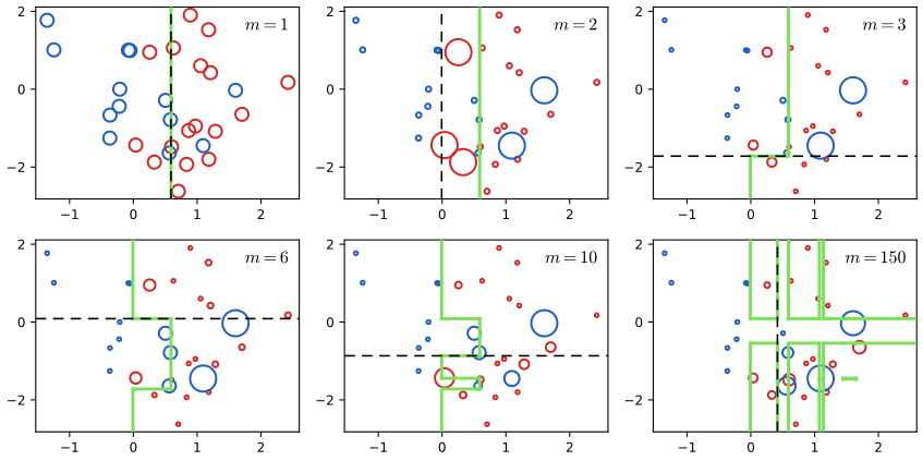
fig14_2() · in the notes · PDF · SVG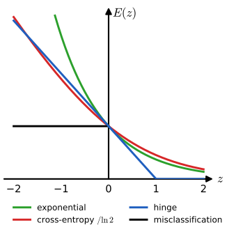
fig14_3() · in the notes · PDF · SVG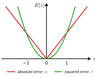
fig14_4() · in the notes · PDF · SVG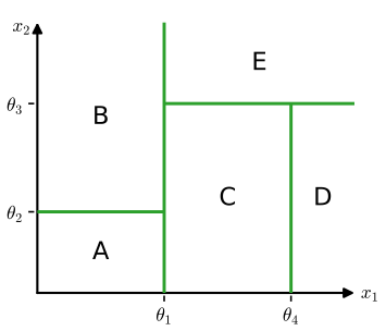
fig14_5() · in the notes · PDF · SVG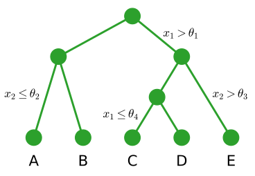
fig14_6() · in the notes · PDF · SVG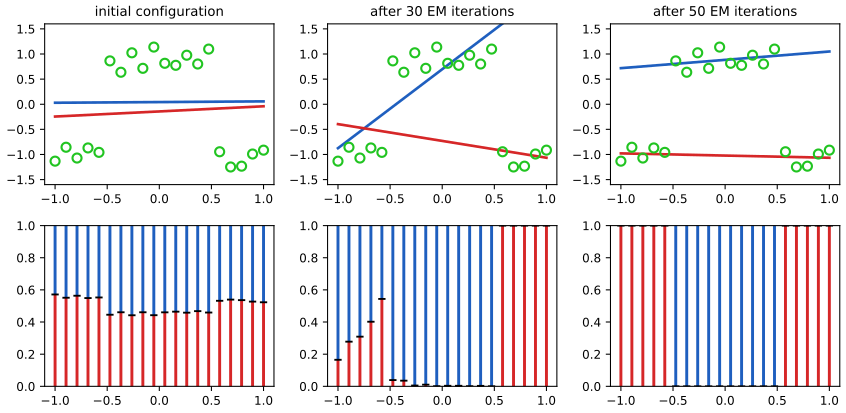
fig14_8() · in the notes · PDF · SVG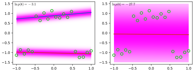
fig14_9() · in the notes · PDF · SVG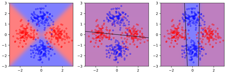
fig14_10() · in the notes · PDF · SVGNumerical checks of the derivations
Each script checks the chapter's derivations numerically (finite-difference gradients, monotone bounds, closed forms against iterative solutions, Monte Carlo against exact moments) and prints a PASS or FAIL line per check.
checks_ch01.py: Numerical checks of the derivations in Bishop (2006), Chapter 1 (Introduction).checks_ch02.py: Numerical checks of the derivations in Bishop (2006), Chapter 2 (Probability Distributions).checks_ch03.py: Numerical checks of the derivations in Bishop (2006), Chapter 3 (Linear Models for Regression).checks_ch04.py: Numerical checks of the derivations in Bishop (2006), Chapter 4 (Linear Models for Classification).checks_ch05.py: Numerical checks of the derivations in Bishop (2006), Chapter 5 (Neural Networks).checks_ch06.py: Numerical checks of the derivations of Chapter 6 (Kernel Methods): prints PASS/FAIL lines.checks_ch07.py: Numerical checks of the derivations in Bishop (2006), Chapter 7 (Sparse Kernel Machines).checks_ch08.py: Numerical checks of the derivations in Bishop (2006), Chapter 8 (Graphical Models).checks_ch09.py: Numerical checks of the derivations in Bishop (2006), Chapter 9 (Mixture Models and EM).checks_ch10a.py: Numerical checks of Bishop (2006), Chapter 10, Sections 10.1 to 10.4, using the functions of ch10_variational_inference.py. Each check prints PASS or FAIL; run `python3 checks_ch10a.py`.checks_ch10b.py: Numerical checks for Bishop (2006), Sections 10.5 to 10.7 (ch10_local_variational_ep.py).checks_ch11.py: Numerical checks of the derivations in Bishop (2006), Chapter 11 (Sampling Methods).checks_ch12.py: Numerical checks of the derivations in Bishop (2006), Chapter 12 (continuous latent variables).checks_ch13.py: Numerical checks of the derivations in Bishop (2006), Chapter 13 (Sequential Data).checks_ch14.py: Numerical checks of the derivations of Bishop (2006), Chapter 14 (Combining models).
Credits
The figures reproduce, with our own code and data, the experiments behind the figures of Bishop, C. M. (2006), Pattern Recognition and Machine Learning, Springer, whose figure numbers are used throughout. Where the book's data or settings are not published, the module notes above say what was used instead. All the code was written from scratch for this course.