Chapter 11. Image data
An image is an array of numbers on a grid, so everything we know about arrays and about statistics applies to it. This chapter follows a fluorescence image of colon cancer cells from raw pixels to a table of cells: smoothing by convolution, thresholding against a local background, cleaning with morphological operations, cutting the foreground into objects and growing each nucleus into a cell body by a Voronoi tessellation on the image. It then changes scale and asks how the positions of hundreds of thousands of immune and tumour cells in a lymph node are arranged in space, using the theory of spatial point processes: the Poisson process as the null model, the intensity, the nearest-neighbour distribution, Ripley's \(K\) and \(L\) functions and the pair correlation function. The notes follow Holmes and Huber (2019), Chapter 11, and write out every step the book leaves to the reader.
Ch. 1 Discrete data Ch. 2 Statistical modeling Ch. 3 Data visualization Ch. 4 Mixture models Ch. 5 Clustering Ch. 6 Testing Ch. 7 Multivariate analysis Ch. 8 Count data and GLMs Ch. 9 Heterogeneous data Ch. 10 Networks and trees Ch. 11 Image data Ch. 12 Supervised learning Ch. 13 Experimental design
How to read these notes
They follow the book. Sections carry the book's numbers (11.8.2, 11.17.1, ...) and the displayed equations of the book carry its numbers, e.g. (11.4), so the notes can be read next to the book. Equations without a number are steps the book skips.
Filling the gaps. The book is an applied text: it uses convolution, morphology, geodesic distances, the Poisson process and Ripley's \(K\) without deriving their properties. Each orange Filling the gap box gives a complete argument at the level of a graduate statistics course; purple boxes state results with proofs. Derivations start hidden: open one with its bar, or use the button below.
Figures, code and demonstrations. Every figure computed from data is reproduced by the R code (ch11_image_data.R). The package spatstat that the book uses for the point-process part was not available, so those estimators are implemented from their definitions and checked against closed forms, brute force and simulation; their numbers can differ slightly from the book's where the book relies on spatstat's defaults. The ▶ Demo boxes open an interactive demonstration already set to the case being discussed.
Main reference
S. Holmes and W. Huber, Modern Statistics for Modern Biology, Cambridge University Press (2019), Chapter 11, "Image data". Section, equation, figure and exercise numbers below refer to this book. Original papers are cited by author and year in the references.
The explanations, derivations and code are my own; equations are cited by their numbers in the book.
The chapter at a glance
- 11.2–11.7 An image is a function on a pixel lattice, stored as an array. Pointwise maps (inversion, contrast, gamma) act on the intensity histogram by a change of variables; geometric maps (rotation, translation, reflection) are computed by inverse mapping and interpolation.
- 11.8 Smoothing is convolution with a weight image. Linear, shift-equivariant filters are exactly the convolutions (Result 11.1), and the discrete Fourier transform turns convolution into multiplication (Result 11.2). A Gaussian of width \(s\) divides the noise standard deviation by about \(2\sqrt\pi s\) at the price of a bias \(\tfrac{s^2}2\Delta f\) (Filling the gap 11.6).
- 11.9–11.11 An adaptive threshold compares each pixel with a local mean; it works when objects are sparse and the background varies slowly (Filling the gap 11.7). Erosion, dilation, opening and closing are Minkowski set operations (Definition 11.3, Result 11.4); objects are connected components.
- 11.12–11.14 Each nucleus grows into a cell body by a Voronoi tessellation for a geodesic distance on the image surface, computed by Dijkstra's algorithm (Algorithm 11.3); \(\lambda\) in (11.4) trades compactness against following the stain. A robust background model gives the cytoplasm threshold; moments of each object give shape features.
- 11.15–11.17 Cell positions form a marked point process. Under complete spatial randomness (a homogeneous Poisson process) the nearest-neighbour distribution is \(1-e^{-\lambda\pi r^2}\) and Ripley's \(K\) is \(\pi r^2\) (Results 11.10, 11.11); edge-corrected estimators are unbiased by the Campbell–Mecke formula (Result 11.12). The T cells of the lymph node avoid each other below about 2 units and cluster beyond.
Notation. Pixels \(p=(x,y)\) run over the lattice \(I=\{1,\dots,n_1\}\times\{1,\dots,n_2\}\), with \(x\) the first array index (horizontal on screen) and \(y\) the second (downwards on screen). An image is \(f:I\to\R\) (or \(\R^c\) for \(c\) colour channels); \(|I|=n_1n_2\). Binary images are subsets \(A\subseteq I\). For point processes, \(W\subset\R^2\) is the observation window with area \(|W|\), \(X\) the random point pattern, \(N(B)\) the number of its points in \(B\), \(\lambda\) the intensity and \(b(u,r)\) the closed disc of radius \(r\) about \(u\).
Prerequisites. The Poisson distribution and Poisson processes in time (Chapter 1), mixture models (Chapter 4), multidimensional scaling (Chapter 9), basic Fourier analysis and kernel density estimation.
11.2 Loading images
The Bioconductor package EBImage (Pau et al. 2010) reads JPEG, PNG and TIFF files with readImage; several files of equal size and colour mode can be read at once and are stacked into one object. Before any processing it helps to say precisely what the object is.
Definition 11.1 (digital image) Sections 11.2, 11.4
A grey-scale image is a function \(f:I\to\R\) on the pixel lattice \(I=\{1,\dots,n_1\}\times\{1,\dots,n_2\}\); a colour image with \(c\) channels is \(f:I\to\R^c\); a stack of \(F\) frames is a list of \(F\) such functions (z-positions, time points, replicates). In R the values are stored as an array of dimension \(n_1\times n_2\) (\(\times\,c\) and/or \(\times\,F\)), \(x\) being the first (fastest) index. A binary image is an indicator \(\ind_A\) of a set \(A\subseteq I\), the foreground. Intensities are real numbers, usually scaled to \([0,1]\); they come from an integer measurement with \(b\) bits, \(f=k/(2^b-1)\) with \(k\in\{0,\dots,2^b-1\}\).
11.3 Displaying images
display shows an image in a browser window or, with method = "raster", on an R graphics device where it can be annotated (Figure 11.1). Screen convention puts the origin at the top left with \(y\) pointing down, the opposite of a Cartesian plot (Question 11.12 below); the figures here follow the screen convention.
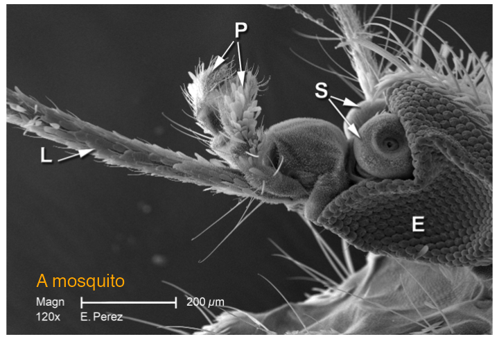
mosquito.png (1400 × 952 grey levels, shown block-averaged by 2) with a text label drawn on top, as display(method = "raster") allows. Image credit: CDC. Reproduces Holmes and Huber (2019), Figure 11.1. Download: PDF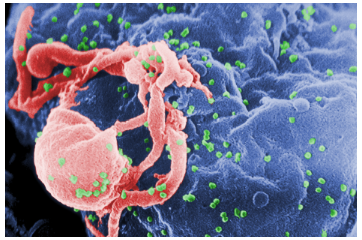
hiv.png, 1400 × 930 × 3, block-averaged by 3. Image credit: CDC. Reproduces Holmes and Huber (2019), Figure 11.2. Download: PDF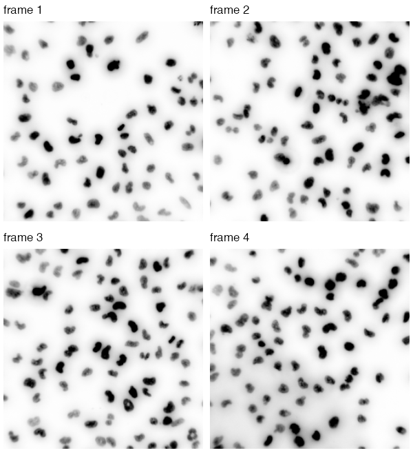
nuclei.tif (510 × 510 × 4, a grey-scale stack) displayed as \(1-f\), so that the bright nuclei appear dark on white. Frame 4 has an uneven background, which motivates Section 11.9. Reproduces Holmes and Huber (2019), Figure 11.3. Download: PDF11.4 How are images stored in R?
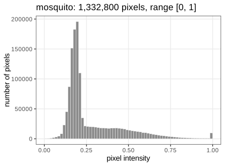
An Image is an R array with two extra slots; arithmetic, indexing and summaries work as on any array. The slot colorMode decides how the third dimension is read: Grayscale treats it as frames, Color as channels (and the fourth dimension as frames). The mosquito is \(1400\times952\) and its values lie on the 8-bit grid \(\{0,\frac1{255},\dots,1\}\); its histogram (Figure 11.4) is the empirical distribution of the \(|I|\) pixel values, with no spatial information at all.
11.5 Writing images to file
R keeps every value as an 8-byte double, so the colour HIV image takes \(1400\cdot930\cdot3\cdot8\) bytes \(\approx29.8\) MB and a 16-megapixel three-channel image \(16\cdot3\cdot8=384\) MB (Question 11.5). Files are compressed: lossless formats (PNG, TIFF with LZW) allow exact reconstruction, lossy ones (JPEG) discard detail the eye barely sees. Scientific images should be stored losslessly. How far lossless compression can go is a statistical question.
Filling the gap 11.1: why lossless compression works, and its limit Section 11.5
The book gives two principles (do not spend more bits than needed; encode patterns by rules). Both are made precise by Shannon's source coding theorem.
Derivation
Model the pixel values as draws of a random symbol \(V\) with probabilities \(p_v\) over an alphabet of size \(m\) (here \(m=256\)). A uniquely decodable binary code with lengths \(\ell_v\) satisfies the Kraft–McMillan inequality \(\sum_v2^{-\ell_v}\le1\). Put \(q_v=2^{-\ell_v}/\sum_u2^{-\ell_u}\). Then
\[ \E[\ell_V]-H(V)=\sum_vp_v\log_2\frac{p_v}{2^{-\ell_v}}=\sum_vp_v\log_2\frac{p_v}{q_v}-\log_2\sum_u2^{-\ell_u}\ \ge\ 0, \]because the first sum is a Kullback–Leibler divergence (non-negative) and the second term is \(\ge0\) by Kraft. So no code beats the entropy \(H(V)=-\sum_vp_v\log_2p_v\) bits per symbol, and Huffman or arithmetic coding come within one bit (within any \(\varepsilon\) for long blocks). Two consequences:
- Fewer bits than stored. \(H\le\log_2m=8\) bits, with equality only for a uniform histogram; a peaked histogram (Figure 11.4) has smaller entropy.
- Patterns. Neighbouring pixels are strongly correlated, so a prediction of each pixel from its neighbours leaves residuals with a much more concentrated distribution. PNG codes the differences to such a prediction. For the mosquito the empirical entropy of the grey levels is 6.62 bits per pixel, that of horizontal differences only 4.26, and the PNG file uses 3.85 bits per pixel: most of the saving comes from the spatial correlation, not from the histogram.
Lossy compression lowers the entropy further by quantising (in JPEG, coarsely rounding the coefficients of a discrete cosine transform), which is irreversible. ∎
11.6 Manipulating images
Because images are arrays, image manipulation is arithmetic. normalize(-mosq) maps \(f\mapsto(\max f-f)/(\max f-\min f)\), inverting bright and dark and rescaling to \([0,1]\) (Question 11.6); mosq * 3 raises the contrast (values above 1 are shown as white); mosq^(1/3) is a gamma correction that brightens dark regions (Figure 11.5). Cropping is array indexing, thresholding gives a logical array, transposition swaps the indices (Figure 11.6).
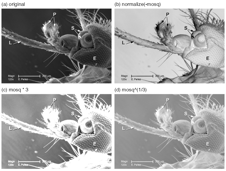
normalize(-mosq), (c) mosq * 3, (d) mosq^(1/3). Reproduces Holmes and Huber (2019), Figure 11.5. Download: PDFFilling the gap 11.2: what a pointwise transformation does to the histogram Section 11.6, Figure 11.5
A pointwise map \(g\) acts on every pixel separately, \(f'(p)=g(f(p))\). It leaves the geometry alone and changes only the distribution of intensities, by the change-of-variables rule.
Derivation
Let \(V\) be the intensity of a pixel chosen uniformly from \(I\), with density \(h_V\) (the smoothed histogram). If \(g\) is strictly increasing and differentiable, \(V'=g(V)\) has distribution function \(F_{V'}(t)=\Prob(V\le g^{-1}(t))\), so its density is
\[ h_{V'}(t)=h_V\big(g^{-1}(t)\big)\,\frac{\d}{\d t}g^{-1}(t)=\frac{h_V(g^{-1}(t))}{g'(g^{-1}(t))}. \]Where \(g'>1\) the histogram is stretched (more contrast), where \(g'<1\) it is compressed. For the gamma map \(g(v)=v^{1/3}\), \(g'(v)=\tfrac13v^{-2/3}\), which exceeds 1 for \(v<3^{-3/2}\approx0.19\): the dark values, where most of the mosquito's background lies, are spread apart, and the bright ones squeezed together, so the image looks brighter and shows more detail in the shadows. For \(g(v)=3v\) the density is \(\frac13h_V(t/3)\) on \([0,3]\), and everything above 1 is clipped on display. The affine normalize only shifts and rescales the histogram. A decreasing \(g\) (inversion) reflects it: \(h_{V'}(t)=h_V(g^{-1}(t))/|g'(g^{-1}(t))|\). ∎
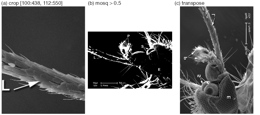
mosq[100:438, 112:550]; (b) thresholding, mosq > 0.5, a logical image (Question 11.7); (c) transposition (Question 11.8). Panels (b) and (c) are block-averaged by 2. Reproduces Holmes and Huber (2019), Figure 11.6. Download: PDF11.7 Spatial transformations
Geometric transformations move pixels rather than change their values: rotate (clockwise by an angle), translate (by a vector; pixels leaving the frame are dropped, new ones are 0), flip and flop (reflections about the horizontal and vertical centre lines), transpose (Figure 11.7).
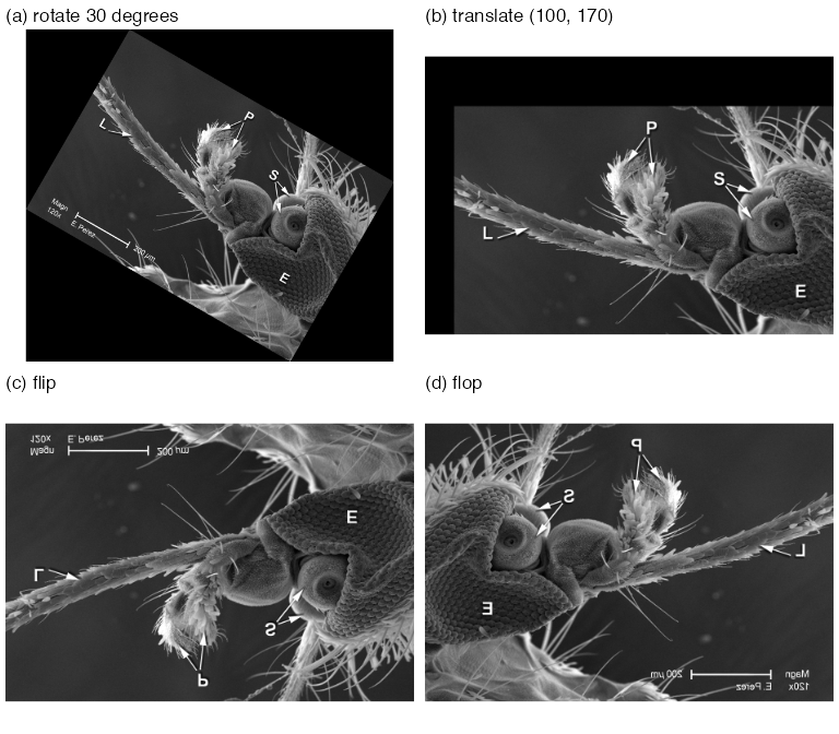
rotate(mosq, 30), on a canvas enlarged to 1688 × 1524; (b) translate(mosq, c(100, 170)) (the book's text uses this vector, its code file c(40, 70)); (c) flip; (d) flop. Block-averaged by 3. Reproduces Holmes and Huber (2019), Figure 11.7. Download: PDFFilling the gap 11.3: rotation by inverse mapping and bilinear interpolation Section 11.7
A rotated pixel centre almost never lands on a pixel centre, so "move each pixel" is not well defined. Rotation is computed backwards.
Derivation
Inverse mapping. For an invertible geometric map \(T\) (here \(Tp=Q(p-c)+c'\) with a rotation matrix \(Q\), centre \(c\) and new centre \(c'\)), define the output at each output pixel \(q\) by \(f'(q)=\tilde f(T^{-1}q)\), where \(\tilde f\) extends \(f\) from the lattice to the plane and is 0 outside the image. Every output pixel gets exactly one value, so there are no holes and no collisions (forward mapping produces both).
Bilinear interpolation. For \(u=(x_0+a,\;y_0+b)\) with integers \(x_0,y_0\) and \(a,b\in[0,1)\),
\[ \tilde f(u)=(1-a)(1-b)f(x_0,y_0)+a(1-b)f(x_0+1,y_0)+(1-a)b\,f(x_0,y_0+1)+ab\,f(x_0+1,y_0+1). \]The weights are non-negative and sum to 1, so \(\tilde f\) stays within the range of its four neighbours, and it reproduces any function of the form \(\alpha+\beta x+\gamma y+\delta xy\) exactly (in particular every affine intensity ramp). Interpolation smooths a little: averaging four noisy pixels lowers the noise variance by the factor \(\sum w_i^2\le1\), with the minimum \(\frac14\) at \(a=b=\frac12\).
Canvas size. Rotating the \(w\times h\) rectangle by \(\theta\) gives a bounding box of width \(w|\cos\theta|+h|\sin\theta|\) and height \(w|\sin\theta|+h|\cos\theta|\) (project the two edge vectors on the axes). For the mosquito and \(\theta=30^\circ\): \(1400\cdot0.866+952\cdot0.5=1688\) and \(1400\cdot0.5+952\cdot0.866=1524\), the dimensions of rotate(mosq, 30).
Exact maps. Flip, flop, transpose and translation by an integer vector are permutations of pixels (composed with cropping), so they need no interpolation and are exactly invertible. ∎
11.8 Linear filters
The working example from here to Section 11.14 is a field of HCT116 human colon cancer cells from a large RNA-interference screen (Laufer et al. 2013), stained for DNA (DAPI), \(\alpha\)-tubulin (FITC) and actin (Cy3). The object cells is \(340\times490\times3\) (Figure 11.8); the full screen has over 690,000 images of \(2048\times2048\) pixels, which is why every step below has to be automatic.
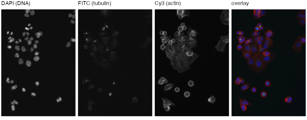
cells after rescaling (Section 11.8.1) and their overlay as red = actin, green = tubulin, blue = DNA. Reproduces Holmes and Huber (2019), Figure 11.8. Download: PDF11.8.1 Interlude: the intensity scale of images
The three TIFF files hold 16-bit integers; readImage returns \(k/65535\). The camera used only the low 11 or 12 bits (the DAPI integers run from 104 to 2045), so the values are small, and the book multiplies the DNA channel by 32 and the others by 16. It remarks that these multiplications do not affect precision.
Filling the gap 11.4: multiplying by a power of two is exact Section 11.8.1
Proof
An IEEE 754 double is \(v=(-1)^s\,m\,2^e\) with a 53-bit significand \(m\in[1,2)\) and an exponent \(e\in[-1022,1023]\). Multiplying by \(2^j\) only changes \(e\) to \(e+j\); \(m\) is untouched, so no rounding happens as long as \(e+j\) stays in range (no overflow, no underflow into subnormals), which holds by far for values in \((10^{-3},1)\) and \(j=5\). Because rounding to the nearest double commutes with scaling by \(2^j\) in that range, \(32\cdot\mathrm{fl}(k/65535)=\mathrm{fl}(32k/65535)\) exactly: the rescaled DAPI channel equals \(q/65535\) with integer \(q=32k\) bit for bit (checked for all 166,600 pixels). This is also why the browser demonstration can be given the integers \(q\) and reproduce the R numbers exactly. Multiplying by 10 instead would round \(m\) and could change the last bit. ∎
11.8.2 Noise reduction by smoothing
To remove pixel-level noise, replace each pixel by an average over a \((2a+1)\times(2a+1)\) window around it, the moving average (11.1), or more generally by a weighted average with weights \(w(s,t)\) that are largest at the centre:
\[ (w*f)(x,y)=\sum_{s=-\infty}^{\infty}\sum_{t=-\infty}^{\infty}w(s,t)\,f(x-s,\,y-t). \tag{11.2} \]Erratum (11.2)
The book prints \(f(x+s,\,y+s)\). The second \(s\) should be \(t\); and with plus signs the sum is a cross-correlation, not a convolution. The convolution, which is what filter2 computes (checked with an asymmetric kernel: filter2 equals \(\sum_sw(s)f(p-s)\) to machine precision and differs from \(\sum_sw(s)f(p+s)\) by up to 0.35), has \(f(x-s,\,y-t)\). The two coincide whenever \(w(s,t)=w(-s,-t)\), as for every brush used in the chapter.
Definition 11.2 (convolution on the image torus) (11.2), filter2
Index the pixels by \(\Z_{n_1}\times\Z_{n_2}\) (coordinates modulo \(n_1\), \(n_2\)). For a weight image \(w\) with finite support, the circular convolution is \((w*f)(p)=\sum_sw(s)f(p-s)\), all coordinates taken modulo the image size. filter2 uses this wrap-around boundary by default; boundary = "replicate" instead extends \(f\) by its edge values. The weight image is called the kernel, brush or filter; it is normalised if \(\sum_sw(s)=1\).
Result 11.1 (convolutions are exactly the linear shift-equivariant filters) Section 11.8.2
(a) \(f\mapsto w*f\) is linear and commutes with translations: if \((\tau_vf)(p)=f(p-v)\) then \(w*(\tau_vf)=\tau_v(w*f)\). It is commutative and associative: \(w*f=f*w\), \((w_1*w_2)*f=w_1*(w_2*f)\). (b) Conversely, every linear map \(L\) on images over \(\Z_{n_1}\times\Z_{n_2}\) that commutes with all translations is a convolution, \(Lf=w*f\) with \(w=L\delta\), the image of a unit impulse \(\delta\) at the origin.
Proof
(a) Linearity is linearity of the finite sum (the book's remark \(w*(c_1f_1+c_2f_2)=c_1w*f_1+c_2w*f_2\)). Shift equivariance: \((w*\tau_vf)(p)\)
(b) Write \(f=\sum_uf(u)\,\tau_u\delta\) (each image is a combination of shifted impulses). By linearity and equivariance, \(Lf=\sum_uf(u)\,\tau_u(L\delta)\), i.e. \((Lf)(p)=\sum_uf(u)\,w(p-u)=(w*f)(p)\) with \(w=L\delta\). The impulse response determines the filter. ∎
Result 11.2 (convolution theorem for the discrete Fourier transform) Section 11.8.2, "filter2 uses the Fast Fourier Transformation"
Let \((\DFT f)(k)\)
Proof
\[ \DFT(w*f)(k)=\sum_p\sum_sw(s)f(p-s)e^{-2\pi i\langle k,p\rangle}=\sum_sw(s)e^{-2\pi i\langle k,s\rangle}\sum_pf(p-s)e^{-2\pi i\langle k,p-s\rangle}=\DFT w(k)\,\DFT f(k), \]because \(p-s\) runs over the whole torus when \(p\) does (this is where the circular boundary is needed; with zero padding to twice the size the same identity gives the non-circular convolution). The inverse transform \(\DFT^{-1}g(p)\)filter2 agrees with the direct circular sum to \(10^{-12}\). ∎
The Gaussian brush makeBrush(51, "gaussian", sigma = 7) is \(w(s,t)\propto\exp\{-(s^2+t^2)/(2\sigma^2)\}\) on \(\{-25,\dots,25\}^2\), normalised to sum 1. Smoothing the DNA channel with it gives Figure 11.9; its middle row is Figure 11.10.
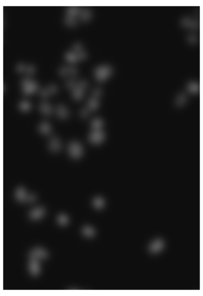
nucSmooth: the DNA channel convolved with the Gaussian brush of \(\sigma=7\) pixels. Reproduces Holmes and Huber (2019), Figure 11.9. Download: PDF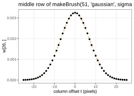
w[26, ] of the brush (points) and the continuous bivariate normal density at the same points, \((2\pi\sigma^2)^{-1}e^{-t^2/(2\sigma^2)}\) (dashed): the discretised, truncated and renormalised brush is almost exactly the density (Filling the gap 11.5). Reproduces Holmes and Huber (2019), Figure 11.10. Download: PDF · SVGFilling the gap 11.5: the Gaussian brush (normalisation, separability, semigroup) Section 11.8.2, Figure 11.10
Derivation
Normalisation. With \(g(t)=e^{-t^2/(2\sigma^2)}\), the brush is \(w(s,t)=g(s)g(t)/Z\), \(Z=(\sum_{|t|\le25}g(t))^2\). By the Euler–Maclaurin formula (or Poisson summation), \(\sum_{t\in\Z}g(t)\)
Separability. \(w=\tilde g\,\tilde g^\T\) with \(\tilde g=g/\sum g\), so \(w*f\) is a convolution along \(x\) followed by one along \(y\): \(2\times51\) instead of \(51^2\) operations per pixel. (The demonstrations use this.)
Semigroup. The Fourier transform of the \(\N(0,\sigma^2)\) density is \(e^{-\sigma^2\omega^2/2}\); products of these are \(e^{-(\sigma_1^2+\sigma_2^2)\omega^2/2}\), so by the convolution theorem two successive Gaussian smoothings equal one with \(\sigma^2=\sigma_1^2+\sigma_2^2\) (in probability language: the sum of independent normal displacements is normal). On the pixel grid this holds up to discretisation: smoothing an impulse with \(\sigma=3\) and then \(4\) agrees with \(\sigma=5\) to \(2\times10^{-5}\). The Fourier transform also shows that a Gaussian filter is a low-pass filter: the frequency \(\omega\) is damped by \(e^{-\sigma^2\omega^2/2}\), so detail at scales below about \(\sigma\) disappears. ∎
Filling the gap 11.6: bias and variance of smoothing Section 11.8.2, "reduced pixel noise, yet still the needed resolution"
Model an observed image as \(f(p)=\mu(p)+\varepsilon(p)\) with a smooth signal \(\mu\) and independent noise of variance \(\tau^2\). For a normalised symmetric kernel \(w\) with \(\sum_sw(s)s s^\T=\sigma^2\mathbf{I}\) (for the Gaussian brush, \(\sigma\) is its parameter),
\[ \var\big((w*f)(p)\big)=\tau^2\sum_sw(s)^2\approx\frac{\tau^2}{4\pi\sigma^2},\qquad \E\big[(w*f)(p)\big]-\mu(p)\approx\frac{\sigma^2}{2}\,\Delta\mu(p). \]Derivation
Variance. \((w*\varepsilon)(p)=\sum_sw(s)\varepsilon(p-s)\) is a weighted sum of independent terms, so its variance is \(\tau^2\sum_sw(s)^2\). For the Gaussian, \(\sum_sw(s)^2\)
Bias. Expand
\[ \mu(p-s)=\mu(p)-s^\T\nabla\mu(p)+\tfrac12s^\T\nabla^2\mu(p)s+O(|s|^3) \] and average with weights \(w\): the constant term is kept (normalisation), the linear term vanishes (symmetry), and the quadratic term gives \(\tfrac12\operatorname{tr}(\sigma^2\mathbf{I}\,\nabla^2\mu)\)
Trade-off. The mean squared error is about \(\tau^2/(4\pi\sigma^2)+\tfrac{\sigma^4}4(\Delta\mu)^2\), minimised at \(\sigma^6=\tau^2/(2\pi(\Delta\mu)^2)\): the noisier the image, the more smoothing pays; the sharper the structures, the less. This is the same bias–variance balance as for kernel density estimation, and it is why the book smooths the small nuclei with \(\sigma=1\) and the broad cytoplasm signals with \(\sigma=3\). ∎
11.9 Adaptive thresholding
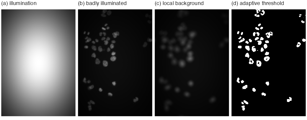
A global threshold \(f(p)>c\) assumes the background has the same level everywhere. With uneven illumination it does not. The adaptive threshold compares each pixel with a local background, the mean over a disc of diameter 21 pixels (larger than a nucleus, smaller than the scale of the illumination):
\[ \text{foreground}=\{p:\ f(p)-(\bar w*f)(p)>\text{offset}\},\qquad \bar w=\text{normalised disc},\ \text{offset}=0.02. \]The book tests it on the DNA channel multiplied by \(\exp\{-(x^2+y^2)\}\) on \([-1,1]^2\) (Figure 11.11): the corners receive \(e^{-2}\approx14\%\) of the central light, yet the peripheral nuclei are found.
Filling the gap 11.7: when does the local mean estimate the background? Section 11.9
The book states the assumption informally ("objects relatively sparse, so the neighbourhood is dominated by background"). Here is what it buys and what it does not.
Derivation
Model \(f(p)=b(p)+\sum_jc_j\ind_{O_j}(p)+\varepsilon(p)\): a slowly varying background \(b\), objects \(O_j\) with contrast \(c_j>0\), noise. Let \(D\) be the disc of \(N_D\) pixels and \(\bar w=\ind_D/N_D\).
Additive background. \((\bar w*f)(p)\)
and in pure background \(\approx-\sum_kc_k\pi_k(p)+\text{noise}\le\text{noise}\). The rule detects a pixel of object \(j\) when \(c_j(1-\pi_j)\) exceeds the offset plus the noise: sparseness (\(\pi_j\) well below 1) is exactly the condition. A disc that fits inside a large object gives \(\pi_j=1\) and the interior is lost; this is why the disc must be larger than the objects, and why the book sees holes in large nuclei (Figure 11.12a). Crowded neighbours (large \(\pi_k\)) lower the difference and split or shrink touching objects.
Multiplicative illumination. With \(f=u\cdot(b+\sum_jc_j\ind_{O_j})\) and \(u\) varying slowly, \(\bar w*f\approx u\cdot\bar w*(\cdot)\), so the difference is about \(u(p)\,c_j(1-\pi_j)\). The illumination cancels in the location of the threshold but not in its scale: a fixed offset is \(1/u(p)\) times larger relative to the signal in dim regions. Dividing instead of subtracting, \(f/(\bar w*f)>1+\delta\), or thresholding \(\log f\), makes the rule invariant to \(u\). With the book's settings, the adaptive threshold on the degraded image finds 51 objects before the opening and 43 after it, the same count as on the original image, while the global threshold 0.2 finds 36 (demo presets 2 and 3).
Mean versus median. The local mean is pulled up by any bright object in the disc (it has breakdown point \(0\)); a local median, or a low quantile, ignores objects covering less than half (or less than the quantile level) of the disc, at a higher computational cost, which is the book's closing remark. ∎
11.10 Morphological operations on binary images
The thresholded image nucThresh has ragged boundaries and isolated pixels. Mathematical morphology (Serra 1983) cleans binary images with a small structuring element \(B\) (a disc of diameter 5 below), using set operations only.
Definition 11.3 (erosion, dilation, opening, closing) Section 11.10
Let \(A\subseteq I\) be the foreground and \(B\subset\Z^2\) a structuring element containing the origin, with reflection \(\check B=\{-b:b\in B\}\) and translates \(A+b\). Then
\[ A\ero B=\{p:\ p+B\subseteq A\}=\bigcap_{b\in B}(A-b),\qquad A\dil B=\{a+b:\ a\in A,\ b\in B\}=\bigcup_{b\in B}(A+b), \] \[ A\circ B=(A\ero B)\dil B\ \ \text{(opening)},\qquad A\bullet B=(A\dil B)\ero B\ \ \text{(closing)}. \]In words: erosion keeps a pixel when the brush placed on it lies entirely in the foreground; dilation sets every pixel the brush reaches from some foreground pixel. In EBImage, brush pixels that fall outside the image are ignored (as if foreground for erosion, background for dilation); with that convention the formulas above reproduce erode, dilate, opening and closing pixel for pixel.
Erratum (the book's description of erode)
The book says: for every foreground pixel, if any pixel under the mask is background, "set all these pixels to background" (and symmetrically for dilate). Taken literally that removes the whole neighbourhood, not just the centre pixel, and it is not erosion: applied to nucThresh (11,433 foreground pixels) with the disc of diameter 5, erosion keeps 5,638 pixels and the worded rule only 1,594. The correct rule changes only the centre pixel, as in Definition 11.3.
Result 11.4 (algebra of the morphological operations) Section 11.10
For a structuring element containing the origin:
- Duality: \((A\dil B)^c=A^c\ero\check B\); for a symmetric \(B\) (the disc), dilation of the foreground is erosion of the background.
- Monotone and (anti-)extensive: \(A\subseteq A'\) implies \(A\ero B\subseteq A'\ero B\) and \(A\dil B\subseteq A'\dil B\); \(A\ero B\subseteq A\subseteq A\dil B\).
- Opening as a union of fits: \(A\circ B=\bigcup\{B+p:\ B+p\subseteq A\}\). Hence \(A\circ B\subseteq A\subseteq A\bullet B\).
- Idempotence: \((A\circ B)\circ B=A\circ B\) and \((A\bullet B)\bullet B=A\bullet B\).
- Not linear: \((A\cup A')\ero B\supseteq(A\ero B)\cup(A'\ero B)\), with strict inclusion in general.
Proof
(1) \(p\notin A\dil B\iff\) for every \(b\in B\), \(p-b\notin A\)
(2) Monotonicity is immediate from the definitions. Since \(0\in B\): \(p+B\subseteq A\) implies \(p\in A\), and \(a=a+0\in A\dil B\).
(3) \(q\in(A\ero B)\dil B\iff q=p+b\) for some \(p\) with \(p+B\subseteq A\) and some \(b\in B\iff q\) lies in a translate \(p+B\) contained in \(A\). Every such translate lies in \(A\), so \(A\circ B\subseteq A\). Closing is the dual: \(A\bullet B=((A^c)\circ\check B)^c\supseteq A\).
(4) By (3), \(A\circ B\) is a union of translates of \(B\), each of which is contained in \(A\circ B\); so every one of them "fits" into \(A\circ B\) and survives a second opening: \((A\circ B)\circ B\supseteq A\circ B\). The reverse inclusion is anti-extensivity. Closing follows by duality.
(5) A pixel whose brush lies partly in \(A\) and partly in \(A'\) survives in \((A\cup A')\ero B\) but in neither erosion. ∎
So opening removes exactly the parts of the foreground into which the brush cannot be fitted (single pixels, spurs, bridges thinner than the disc) and leaves everything else untouched; closing fills gaps and holes the brush cannot enter. For nucThresh the opening with the 5-pixel disc removes 241 of 11,433 pixels (Figure 11.12b).
11.11 Segmentation of a binary image into objects
nucOpened separates foreground from background but not one nucleus from another. bwlabel numbers the connected components.
Definition 11.4 (connectivity and connected components) Section 11.11
Two pixels are 4-adjacent if they differ by one unit in one coordinate, 8-adjacent if they differ by at most one unit in each. A path in \(A\) is a sequence of pixels of \(A\), each adjacent to the next; "joined by a path in \(A\)" is an equivalence relation, and its classes are the connected components of \(A\). bwlabel uses 4-adjacency (two pixels touching only at a corner are separate objects) and numbers the components in the order of their first pixel in column-major order; it returns an integer image with 0 for background. On nucOpened it finds 43 objects (8-adjacency would merge a few of them).
Algorithm 11.1 (labelling connected components) Section 11.11, bwlabel
- Set \(L(p)=0\) for all \(p\) and \(n=0\).
- Scan the pixels in storage order. At a foreground pixel with \(L(p)=0\), set \(n\leftarrow n+1\), \(L(p)=n\), and put \(p\) in a queue.
- While the queue is not empty, remove a pixel \(q\); for each 4-neighbour \(q'\in A\) with \(L(q')=0\), set \(L(q')=n\) and add \(q'\) to the queue.
- Return \(L\) and the number of objects \(n\). The table of \(L\) gives the object areas in pixels (Question 11.10).
Each pixel enters the queue once, so the cost is \(O(|I|)\). (Two-pass union–find algorithms do the same with less memory.) Breadth-first search visits exactly the pixels joined to the seed by a path, so the labels are the equivalence classes of Definition 11.4.
Two kinds of error remain: touching nuclei that were not separated, and nuclei with holes. The book's fix is to build a lenient mask, nucMask \(=\{f-\bar w*f>0\}\) with its holes filled by fillHull, and to grow the 43 labelled seeds within it by the propagation of Section 11.12.
Filling the gap 11.8: what is a hole? Section 11.11, fillHull
Definition and the connectivity pairing
A hole of \(A\) is a connected component of the background \(A^c\) that does not touch the border of the image; fillHull adds all holes to \(A\). Which adjacency to use for the background matters. Take a foreground ring that is closed only through corner contacts: with 4-adjacency it is not a closed curve, so its inside leaks out through the diagonal gaps if the background is 8-connected, yet it is "enclosed" if the background is 4-connected. Digital topology (Rosenfeld 1970) resolves the paradox by pairing the adjacencies: the digital Jordan curve theorem holds for (foreground 8, background 4) and for (foreground 4, background 8), not for (4, 4) or (8, 8). EBImage's fillHull treats the background as 4-connected: holes computed this way reproduce it pixel for pixel on nucMask, while 8-connected background components give a different result (3,825 pixels differ).
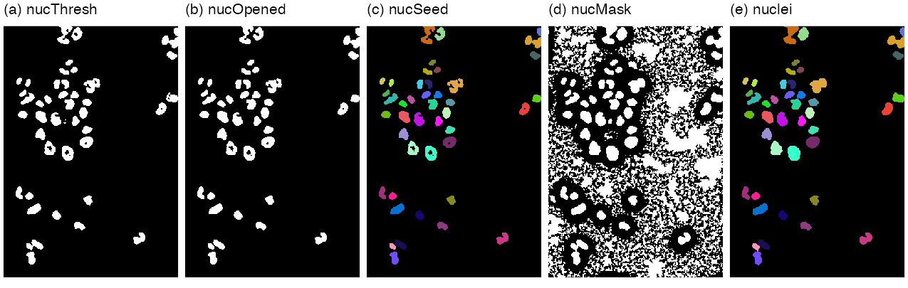
nucThresh, (b) nucOpened, (c) nucSeed (43 labels, random colours), (d) nucMask after fillHull, (e) nuclei, the seeds propagated within the mask. Reproduces Holmes and Huber (2019), Figure 11.12. Download: PDFAlgorithm 11.2 (the nuclear segmentation pipeline of Sections 11.8 to 11.11)
- Rescale: \(f\leftarrow32f\) (exact, Filling the gap 11.4).
- Smooth: \(f_s=w_{\sigma=1}*f\) with the \(51\times51\) Gaussian brush, circular boundary.
- Threshold: \(T=\{f_s-\bar w_{21}*f_s>0.02\}\), \(\bar w_{21}\) the normalised disc of diameter 21. (11,433 pixels.)
- Open: \(O=T\circ B_5\), \(B_5\) the disc of diameter 5. (11,192 pixels.)
- Label: \(S=\) connected components of \(O\) (4-adjacency). (43 objects.)
- Mask: \(M=\) holes of \(\{f_s-\bar w_{21}*f_s>0\}\) filled.
- Grow: \(\text{nuclei}=\) propagate the labels of \(S\) within \(M\) over \(f_s\) with \(\lambda=10^{-4}\) (Algorithm 11.3).
The browser demonstration runs steps 1 to 5 and reproduces the three counts exactly.
11.12 Voronoi tessellation
Definition 11.5 (Voronoi tessellation for a distance) Section 11.12
Let \(S_1,\dots,S_m\) be disjoint seed sets in a space \(\Omega\) with a distance \(d\). The Voronoi cell of seed \(j\) is \(V_j\)
Result 11.5 (Euclidean Voronoi cells of points are convex polygons)
For point seeds \(s_1,\dots,s_m\) in \(\R^2\) and Euclidean distance,
\[ V_j=\bigcap_{k\ne j}\{u:\ \langle u,s_k-s_j\rangle\le\tfrac12(|s_k|^2-|s_j|^2)\}, \]an intersection of half-planes bounded by the perpendicular bisectors.
Proof
\(|u-s_j|^2\)
Seeds that are regions (the nuclei) or a non-Euclidean distance lose this: cells can be non-convex, as in Figure 11.13 where the seeds are whole nuclei.
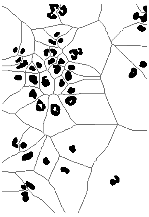
propagate(seeds = nuclei, x = zeros, lambda = 100). Reproduces Holmes and Huber (2019), Figure 11.13. Download: PDFThe book's second generalisation measures distance on the surface \(z=\tilde f(x,y)\) given by an image \(\tilde f\). For neighbouring points \((x,y,z)\) and \((x+\d x,y+\d y,z+\d z)\), the flat metric (11.3) \(\d s^2=\d x^2+\d y^2\) is replaced by
\[ \d s^2=\frac{2}{\lambda+1}\big[\lambda(\d x^2+\d y^2)+\d z^2\big],\qquad\lambda\ge0, \tag{11.4} \]with the limits \(\lambda=1\): \(\d s^2=\d x^2+\d y^2+\d z^2\); \(\lambda=0\): \(\d s^2=2\,\d z^2\); \(\lambda\to\infty\): \(\d s^2=2(\d x^2+\d y^2)\) (11.5). The distance between two points is the infimum of \(\int\d s\) over paths joining them, a geodesic distance; the book calls the surface with this metric a Riemannian manifold.
Filling the gap 11.9: the metric (11.4), its limits, and what EBImage computes (11.3)–(11.5)
Derivation
As a Riemannian metric. On the surface \(z=\tilde f(x,y)\), \(\d z=\tilde f_x\d x+\tilde f_y\d y\), so (11.4) is the quadratic form \(\d s^2\)
The limits (11.5) follow by substitution: \(\lambda=1\) gives the factor \(2/2=1\); \(\lambda=0\) gives \(2\,\d z^2\); for \(\lambda\to\infty\), \(\frac{2\lambda}{\lambda+1}\to2\) and \(\frac{2}{\lambda+1}\to0\). The constant factor \(2/(\lambda+1)\) does not change which seed is nearest, so the tessellation depends on \(\lambda\) only through the ratio of lateral to vertical cost. With \(\lambda=100\) on a flat image (\(\d z\equiv0\)) every \(\lambda\) gives the same result, the ordinary Voronoi tessellation (Figure 11.13).
Discretisation. On the pixel grid, paths are sequences of 8-neighbours, and a step from \(p\) to \(q\) costs \(\sqrt{(\d z^2+\lambda|p-q|^2)/(1+\lambda)}\) (the factor 2 dropped). Reimplementing this in R, I found that EBImage's propagate takes for \(\d z\) not \(\tilde f(q)-\tilde f(p)\) but the sum over the \(3\times3\) window of \(|\tilde f(p+e)-\tilde f(q+e)|\), \(e\in\{-1,0,1\}^2\) (edges replicated), a smoothed gradient: with this choice the reimplementation reproduces propagate on every pixel, for the nuclei (\(\lambda=10^{-4}\)) and for the cell bodies (\(\lambda=10^{-2}\)); with the plain difference, 96.7% of cell-body pixels agree. On the flat image of Figure 11.13 the two implementations differ on 92 of 166,600 pixels, where two seeds are at exactly the same path length and the tie is broken differently. On the grid the flat distance is the 8-neighbour path length (steps 1 and \(\sqrt2\)), not the Euclidean distance; the resulting Voronoi tessellation agrees with the exact Euclidean one (nearest nuclear pixel) on 97.6% of the pixels, the differences lying along cell boundaries. ∎
Algorithm 11.3 (Voronoi propagation by Dijkstra's algorithm) Section 11.12, propagate (Jones et al. 2005)
- Nodes: the pixels of the mask \(M\) (and of the seeds). Edges: pairs of 8-neighbours in \(M\), with the step cost \(c(p,q)>0\) above.
- Set \(D(p)=0\) for seed pixels, \(D(p)=\infty\) otherwise; put all seed pixels in a priority queue.
- Repeat until the queue is empty: remove the pixel \(p\) with the smallest \(D\), mark it final, and for each neighbour \(q\) not final, if \(D(p)+c(p,q)<D(q)\) set \(D(q)\leftarrow D(p)+c(p,q)\) and (re)insert \(q\).
- Label each pixel with the label of the seed at the start of its shortest path (equivalently: in order of increasing \(D\), copy the label of the neighbour \(q\) minimising \(D(q)+c(q,p)\)). Pixels of \(M\) not reachable from any seed stay 0.
With a binary heap the cost is \(O(|E|\log|M|)\); for the cell image about 0.15 s in a browser.
Result 11.6 (Dijkstra's algorithm computes the geodesic Voronoi tessellation)
For positive step costs, when a pixel \(p\) is removed from the queue, \(D(p)\) equals the length of a shortest path from the seed set to \(p\); consequently the labels of step 4 assign each pixel to a nearest seed in the discrete geodesic distance.
Proof
Adding a virtual source joined to every seed pixel at cost 0 turns the multi-source problem into a single-source one. Induction on the removals: suppose all previously removed pixels have correct distances, and \(p\) is removed with \(D(p)>\delta(p)\), the true distance. Take a shortest path to \(p\) and its first pixel \(q\) not yet removed, with predecessor \(q^-\) on the path already removed. When \(q^-\) was removed, \(q\) was relaxed, so \(D(q)\)
11.13 Segmenting the cell bodies
To find the cytoplasm, the book thresholds the smoothed tubulin and actin channels globally, using a model of the log-intensity histogram (Figures 11.14, 11.15): a large log-normal background component and a flat, mostly non-overlapping foreground component to its right.
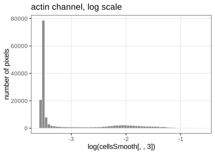
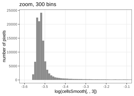
The function bgPars takes, on the log scale, the location loc = half-range mode, the width wid = root mean square of the deviations of the values left of the mode, and the threshold thr = loc + 6 wid. For actin: loc \(=-3.5219\), wid \(=0.01528\), thr \(=-3.4302\), exactly as in the book.
Filling the gap 11.10: the robust background estimates and the 6-width threshold Section 11.13, bgPars, footnote 11
Derivation
Model. The log intensity of a pixel has density \(h(v)=\pi_0\,\varphi_\sigma(v-\mu)+(1-\pi_0)h_1(v)\), with \(\varphi_\sigma\) the \(\N(0,\sigma^2)\) density, \(\pi_0\) large, and the foreground density \(h_1\) essentially zero on \((-\infty,\mu]\).
Location. The half-range mode (Bickel 2002) repeatedly keeps the shortest interval containing half of the remaining sample until a few points are left, and returns their midpoint. Because \(\pi_0\varphi_\sigma\) is symmetric and dominant, the densest region of \(h\) is centred at \(\mu\) and the shortest-half intervals converge on it; the foreground tail cannot move them unless it adds mass inside the interval. (Simulation: a \(\N(2,0.5^2)\) sample contaminated by 17% uniform values on \([3,6]\) gives a half-range mode within 0.03 of 2, while the mean moves to 2.42.)
Width. If \(V\sim\N(\mu,\sigma^2)\), then by symmetry \(\E[(V-\mu)^2\given V<\mu]\)wid \(=\{\frac1{n_-}\sum_{v_i<\hat\mu}(v_i-\hat\mu)^2\}^{1/2}\). (Simulation: \(0.500\) for \(\sigma=0.5\) from \(10^6\) draws.)
Threshold. A background pixel exceeds \(\mu+6\sigma\) with probability \(1-\Phi(6)=9.9\times10^{-10}\); among the 166,600 pixels the expected number of false foreground pixels is \(1.6\times10^{-4}\), if the background were exactly normal. In practice tails are heavier than normal and neighbouring pixels are correlated after smoothing, so the factor 6 is a safety margin, as the book's footnote says.
The model-based alternative of footnote 11. With estimates of \(\pi_0\), \(\mu\), \(\sigma\) and a model for \(h_1\) (for instance flat on the observed range, or a second normal fitted by EM as in Chapter 4), assign pixel \(v\) to the foreground when its posterior probability exceeds \(\frac12\):
\[ \Prob(\text{fg}\given v)=\frac{(1-\pi_0)h_1(v)}{\pi_0\varphi_\sigma(v-\mu)+(1-\pi_0)h_1(v)}>\tfrac12\iff\frac{(v-\mu)^2}{2\sigma^2}>\log\frac{\pi_0}{(1-\pi_0)h_1(v)\sqrt{2\pi}\sigma}. \]For a flat \(h_1\) the threshold is \(\mu+\sigma\sqrt{2\log\{\pi_0/((1-\pi_0)h_1\sqrt{2\pi}\sigma)\}}\), which adapts to how much foreground there is instead of using a fixed 6. ∎
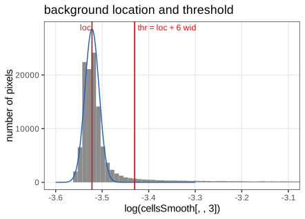
loc (brown) and thr (red); the blue curve is the normal background \(\N(\text{loc},\text{wid}^2)\) scaled to twice the number of pixels left of the mode (my addition), which fits the left half of the peak by construction and shows how far the right tail exceeds it. Reproduces Holmes and Huber (2019), Figure 11.16. Download: PDF · SVGThe cytoplasm mask is the union of the pixels above threshold in the tubulin or the actin channel and the nuclei. Within it, the nuclei are propagated over the actin channel with \(\lambda=0.01\): each nucleus gets exactly one cell body, and the boundaries compromise between compact shapes and the actin signal (Figure 11.17).
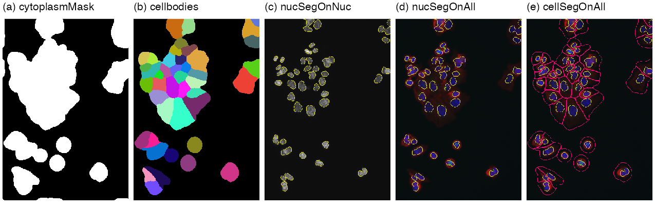
cytoplasmMask, (b) cellbodies in random colours, (c) nuclear outlines on the DNA channel, (d) on the colour overlay, (e) cell-body outlines added. Reproduces Holmes and Huber (2019), Figure 11.17 (whose caption says "(a-d)" for its five panels). Download: PDF11.14 Feature extraction
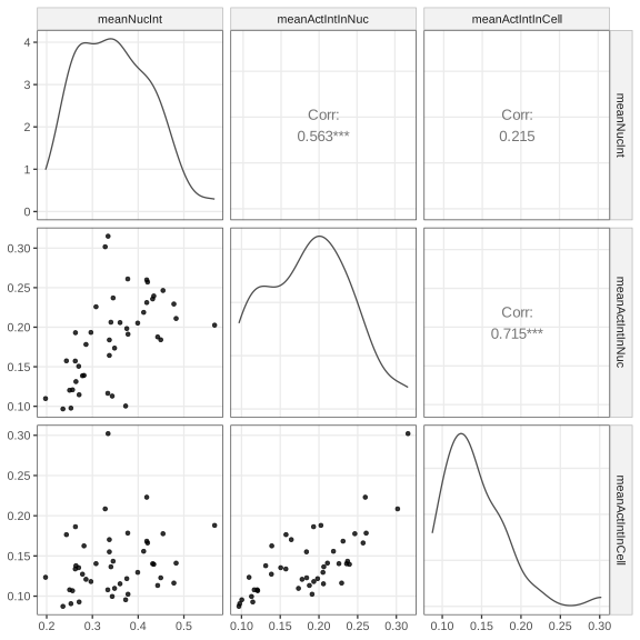
With the two segmentations, any summary of the pixels of an object is a feature: the mean DNA intensity in the nucleus, the mean actin intensity in the nucleus and in the cell body (Figure 11.18), or the 89 features per object that computeFeatures returns (moments, shape, intensity quantiles, Haralick texture).
Filling the gap 11.11: moment features (centroid, major axis, eccentricity, orientation) Section 11.14, computeFeatures
The first five columns of F1 (m.cx, m.cy, m.majoraxis, m.eccentricity, m.theta) are functions of the first two moments of the pixel coordinates of each object, the "ellipse of inertia".
Derivation
For an object \(O\) with \(n\) pixels, let \(\bar p=\frac1n\sum_{p\in O}p\) (the centroid, cx, cy) and \(S=\frac1n\sum_{p\in O}(p-\bar p)(p-\bar p)^\T\) with eigenvalues \(\ell_1\ge\ell_2\) and leading eigenvector \(e_1\). For a filled ellipse with semi-axes \(a\ge b\), the uniform distribution on it has \(S=\diag(a^2/4,\,b^2/4)\) in its own axes: with \(x=a\rho\cos\phi\), \(y=b\rho\sin\phi\) and area element \(ab\rho\,\d\rho\,\d\phi\),
So the ellipse with the same moments as \(O\) has full major axis \(2a=4\sqrt{\ell_1}\) (majoraxis), eccentricity \(\sqrt{1-b^2/a^2}=\sqrt{1-\ell_2/\ell_1}\) (eccentricity, 0 for a disc, near 1 for an elongated object), and orientation the angle of \(e_1\), reduced to \((-\pi/2,\pi/2]\) (theta). These formulas reproduce computeFeatures for all 43 nuclei to \(10^{-6}\) (with the divisor \(n\), not \(n-1\)); the first nucleus has centroid \((119.55,17.47)\), major axis 44.87, eccentricity 0.837. ∎
Feature tables can then be analysed with the multivariate methods of earlier chapters (PCA, clustering, classification), and with the cells' positions, which is where the chapter turns next.
11.15 Spatial statistics: point processes
From here on the data are positions of cells, not pixels.
Definition 11.6 (point process, marks, window) Section 11.15
A spatial point process \(X\) on \(\R^2\) is a random locally finite set of points; equivalently its counting measure \(N(B)=\#(X\cap B)\), a random variable for every bounded Borel set \(B\). A marked point process attaches a mark (here the cell type) to every point. We observe one realisation inside a window \(W\); the choice of \(W\) is part of the model, since "no points here" means something different inside and outside it.
11.15.1 A case study: interaction between immune cells and cancer cells
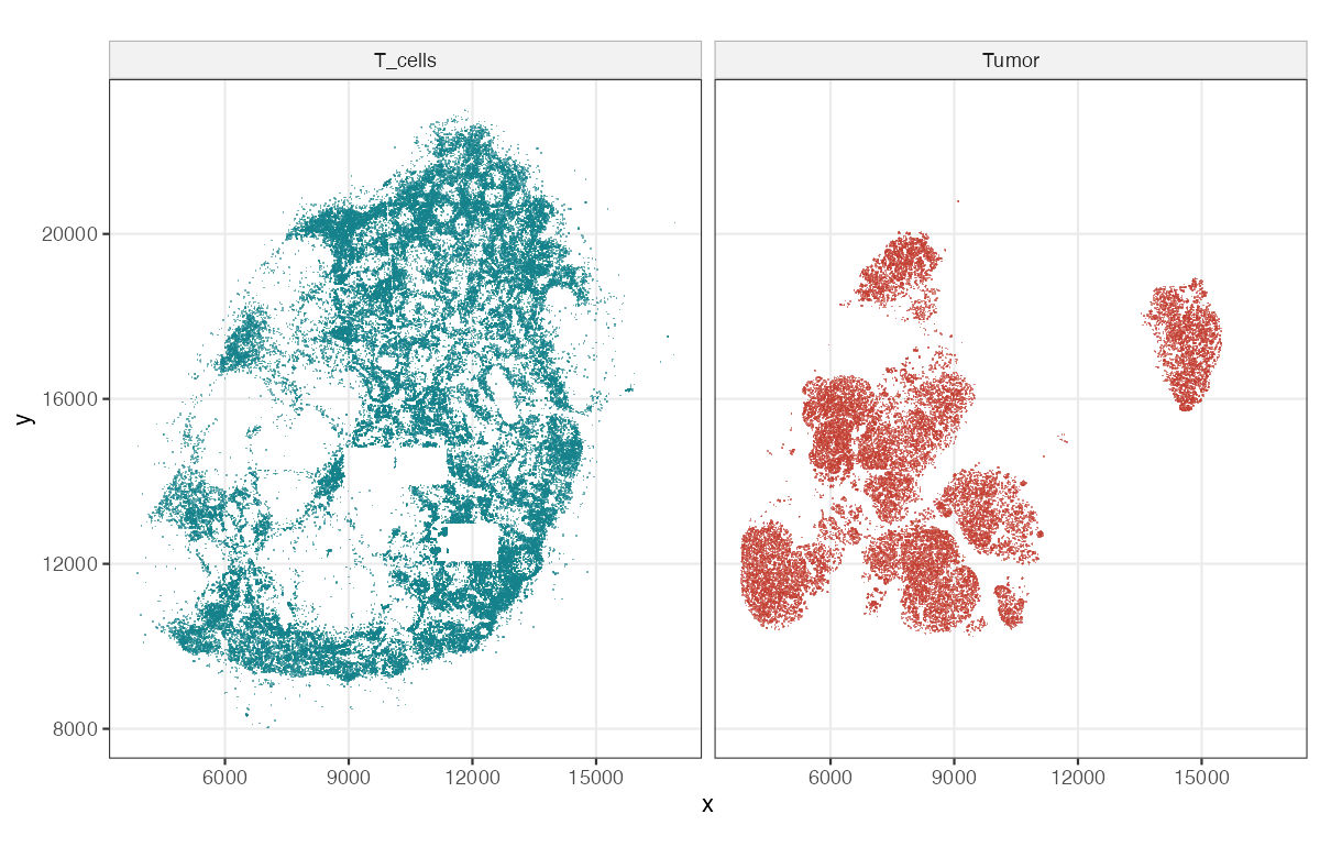
Setiadi et al. (2010) segmented a stained section of a sentinel lymph node from a breast-cancer patient (with the GemIdent software, Holmes et al. 2009) into 209,462 cells: 103,681 T cells, 27,822 tumour cells, 878 dendritic cells and 77,081 others. Figure 11.21 shows the T cells and the tumour cells; Figures 11.19 and 11.20 of the book (photographs of a biopsy and of the stained section) are not reproduced.
11.15.2 Convex hull
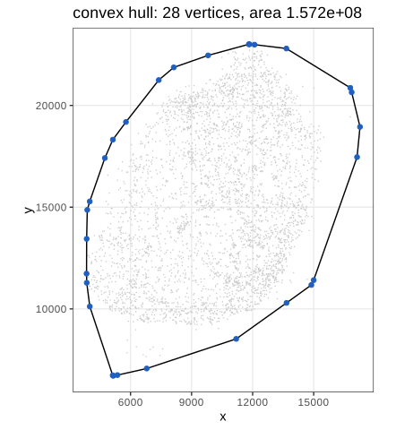
The bounding rectangle \([3839,17276]\times[6713,23006]\) contains large empty corners. A tighter window is the convex hull of all 209,462 points, the smallest convex set containing them: a polygon with 28 vertices and area \(1.572\times10^8\) (Figure 11.22). It can be computed in \(O(n\log n)\) by sorting the points by \(x\) and building the lower and upper chains with a stack, discarding a point whenever the last three make a clockwise turn (Andrew's monotone chain; R's chull). A useful consequence: \(\sqrt{1000/(\pi\hat\lambda_T)}=694.70\) with \(\hat\lambda_T=103{,}681/|W|\), exactly the upper limit of \(r\) in the book's Figure 11.28, which confirms that the window is the same.
11.15.3 Other ways of defining the space for the point process
The window can also be a mask from prior knowledge (the tissue outline), or a region where a kernel density estimate of the points is high enough. The hull overstates the observed region where the boundary is concave and includes unobserved tiles (the rectangles of Figure 11.21); every estimator below divides by an area or uses distances to the boundary, so such choices matter.
11.16 First order effects: the intensity
Do points attract or repel each other, and at which scale? To answer, we need what to expect "by chance". With \(N(p,a)\) the number of points in a disc of area \(a\) about \(p\), the book defines the intensity
\[ \lambda(p)=\lim_{a\to0}\frac{\E[N(p,a)]}{a}, \tag{11.6} \]and the spatial covariance
\[ \gamma(p_1,p_2)=\lim_{a\to0}\frac{\E\big[(N(p_1,a)-\E N(p_1,a))(N(p_2,a)-\E N(p_2,a))\big]}{a^2}. \tag{11.7} \]A process is stationary if its distribution is invariant under translations (then \(\lambda\) is constant and \(\E N(B)=\lambda|B|\)), and isotropic if also under rotations.
Result 11.8 (Campbell's formulas)
If \(X\) has intensity function \(\lambda(u)\), then for every measurable \(h\ge0\),
\[ \E\sum_{x\in X}h(x)=\int h(u)\lambda(u)\,\d u. \]If \(X\) has a second-order intensity \(\rho^{(2)}(u,v)\), defined by \(\E[N(A)N(B)]-\E N(A\cap B)\)
Proof
For \(h=\ind_B\) the first formula is the definition of \(\lambda\) (\(\E N(B)=\int_B\lambda\)). Both sides are linear in \(h\), so it holds for simple functions, and by monotone convergence for every \(h\ge0\). For the second, \(\sum_x\sum_{y\ne x}\ind_A(x)\ind_B(y)\)
Filling the gap 11.12: the spatial covariance (11.7) has a singular part (11.6), (11.7)
Derivation
Write \(B_i=b(p_i,\cdot)\) for the two small discs of area \(a\). Using the definition of \(\rho^{(2)}\) in Result 11.8,
\[ \cov(N(B_1),N(B_2))=\int_{B_1}\!\int_{B_2}\big[\rho^{(2)}(u,v)-\lambda(u)\lambda(v)\big]\d u\,\d v+\int_{B_1\cap B_2}\lambda(u)\,\d u. \]For \(p_1\ne p_2\) the discs are eventually disjoint, the last term vanishes, and dividing by \(a^2\) gives \(\gamma(p_1,p_2)\)
11.16.1 Poisson Process
Definition 11.7 (Poisson process; complete spatial randomness) Section 11.16.1
A Poisson process with intensity function \(\lambda(u)\) has (i) \(N(B)\sim\Pois\big(\int_B\lambda\big)\) for every bounded \(B\), and (ii) independent counts \(N(B_1),\dots,N(B_k)\) for disjoint sets. It is homogeneous if \(\lambda\) is constant; the homogeneous Poisson process is the model of complete spatial randomness (CSR). The book's figure of rain drops (Figure 11.23) illustrates it.
Result 11.9 (conditional uniformity, simulation, moments)
For a homogeneous Poisson process on \(W\): given \(N(W)=n\), the \(n\) points are independent and uniformly distributed on \(W\). Hence it can be simulated by drawing \(n\sim\Pois(\lambda|W|)\) and then \(n\) uniform points. \(\E N(B)=\var N(B)=\lambda|B|\), \(\rho^{(2)}(u,v)=\lambda^2\), and \(\gamma(p_1,p_2)=0\) for \(p_1\ne p_2\).
Proof
Partition \(W\) into \(B_1,\dots,B_k\) and let \(n_1+\dots+n_k=n\). By (i) and (ii),
\[ \Prob(N(B_j)=n_j\ \forall j\given N(W)=n)=\frac{\prod_je^{-\lambda|B_j|}(\lambda|B_j|)^{n_j}/n_j!}{e^{-\lambda|W|}(\lambda|W|)^n/n!}=\frac{n!}{\prod_jn_j!}\prod_j\Big(\frac{|B_j|}{|W|}\Big)^{n_j}, \]the multinomial distribution of \(n\) independent uniform points. Since the counts in all finite partitions determine the distribution of a point process, the claim follows. The moments: a Poisson count has mean = variance; for disjoint \(A,B\), \(\E N(A)N(B)=\lambda^2|A||B|\), giving \(\rho^{(2)}=\lambda^2\) and \(\gamma=0\) off the diagonal (Filling the gap 11.12). Checked by simulation: counts in a \(30\times30\) square have mean and variance both within 8% of \(\lambda|B|=18\), and counts in disjoint squares are uncorrelated. ∎
11.16.2 Estimating the intensity
The intensity is estimated like a density, with a kernel \(K_\sigma\) (here Gaussian with standard deviation \(\sigma\)) and an edge correction:
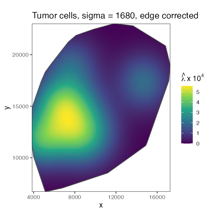
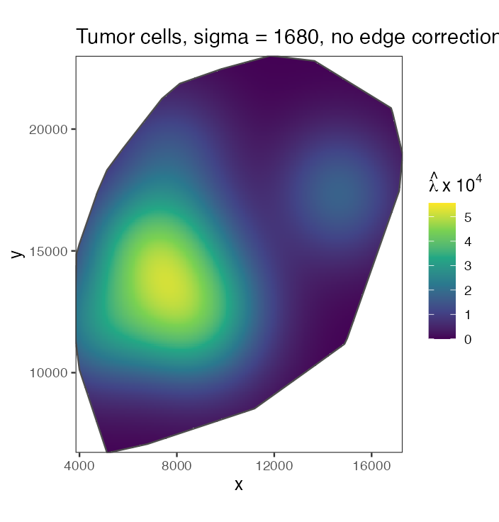
\[ \hat\lambda(p)=\sum_ie(p_i)\,K_\sigma(p-p_i). \tag{11.8} \]Figure 11.24 shows the tumour-cell intensity with \(\sigma\) one eighth of the shorter side of the bounding rectangle (\(\sigma\approx1680\)); Figure 11.25 the same without edge correction.
Filling the gap 11.13: what the edge correction corrects (11.8), Figures 11.24, 11.25
Let \(e_W(u)=\int_WK_\sigma(u-v)\,\d v\), the mass of the kernel centred at \(u\) that lies in the window. The book's \(e(p_i)\) in (11.8) is the weight \(1/e_W(p_i)\) (Diggle 1985); the alternative "uniform" correction divides the whole estimate by \(e_W(p)\).
\[ \hat\lambda_0(p)=\sum_iK_\sigma(p-p_i),\qquad \hat\lambda_U(p)=\frac{\hat\lambda_0(p)}{e_W(p)},\qquad \hat\lambda_D(p)=\sum_i\frac{K_\sigma(p-p_i)}{e_W(p_i)}. \]Derivation
Only points inside \(W\) are observed, so the sums run over \(X\cap W\). By Campbell's formula,
\[ \E\hat\lambda_0(p)=\int_WK_\sigma(p-v)\lambda(v)\,\d v,\qquad \E\hat\lambda_D(p)=\int_WK_\sigma(p-v)\frac{\lambda(v)}{e_W(v)}\,\d v. \]For a constant \(\lambda\): \(\E\hat\lambda_0(p)=\lambda e_W(p)\), which falls to about \(\lambda/2\) on a straight edge and \(\lambda/4\) at a right-angled corner (when \(\sigma\) is small compared with the window): the uncorrected estimate fades towards the boundary (Figure 11.25). Dividing by \(e_W(p)\) gives \(\E\hat\lambda_U(p)=\lambda\) exactly. Diggle's estimator is instead mass-preserving: each point's kernel has mass \(e_W(p_i)\) inside \(W\), so \(\int_W\hat\lambda_D(p)\,\d p=\sum_ie_W(p_i)/e_W(p_i)=n\), the observed count, for every pattern. Pointwise it is not unbiased at the boundary: for constant \(\lambda\), \(\E\hat\lambda_D(p)\)
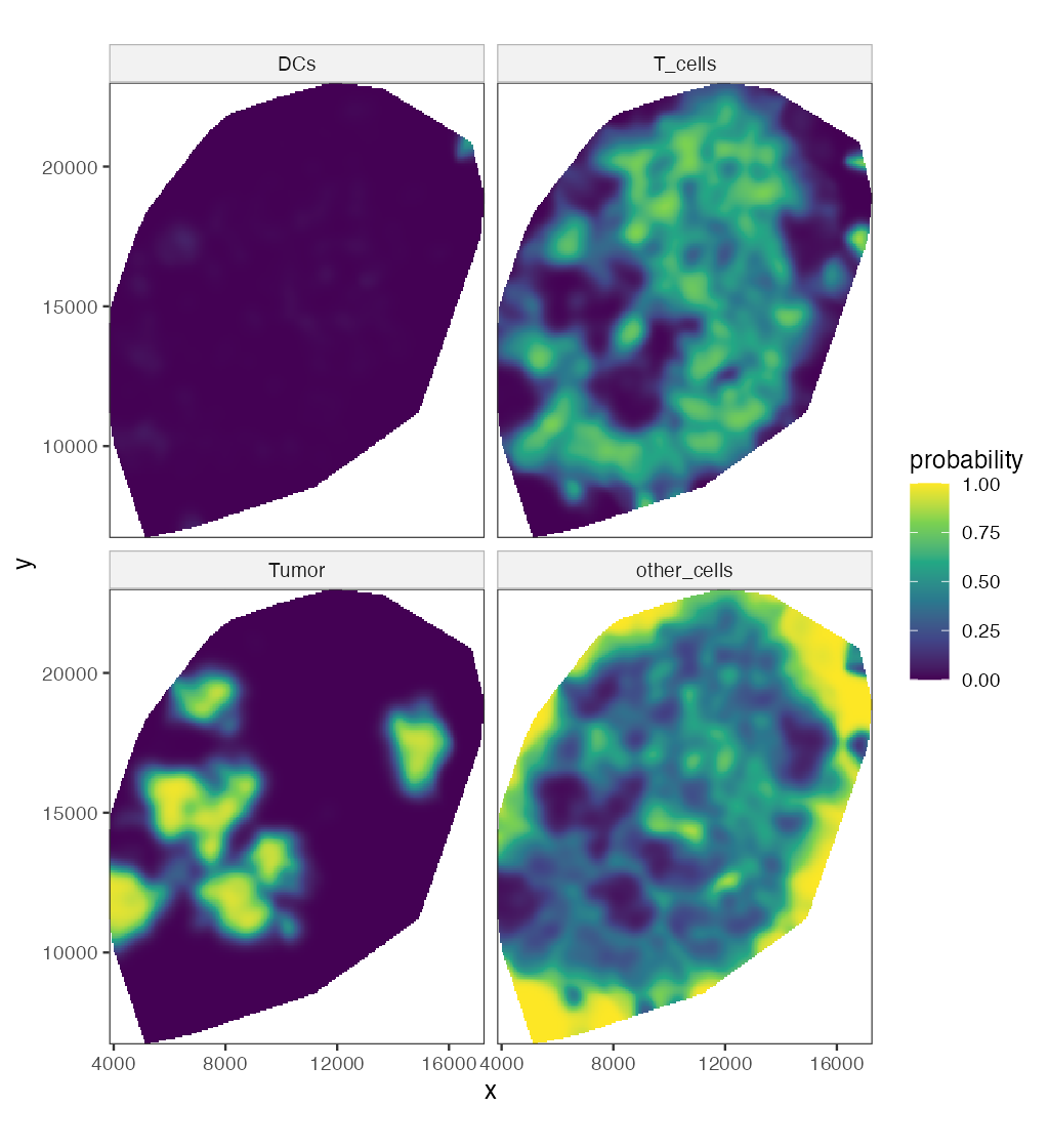
The relative risk of each cell type is the ratio of its smoothed intensity to the total (Figure 11.26, \(\sigma=250\)).
Filling the gap 11.14: relative risk is a conditional probability of the mark Figure 11.26, relrisk
Derivation
For a multitype process with type-\(k\) intensities \(\lambda_k(u)\), the unmarked process has intensity \(\lambda(u)=\sum_k\lambda_k(u)\). The probability that a point in a small disc \(b(u,\varepsilon)\) has mark \(k\), given that there is a point there, is \(\E N_k(b)/\E N(b)\to\lambda_k(u)/\lambda(u)=:p_k(u)\) as \(\varepsilon\to0\) (for small discs the counts are 0 or 1, as in Filling the gap 11.12). The estimate \(\hat p_k=\hat\lambda_k/\sum_j\hat\lambda_j\) with the same kernel for all types sums to one at every location, and any edge factor \(1/e_W(u)\) cancels in the ratio, so no edge correction is needed. It is a Nadaraya–Watson regression of the indicator "type \(k\)" on location. Far from all cells the numerator and the denominator are both at the level of floating-point round-off, so the ratio is computed only where the total intensity is above \(10^{-9}\) of its maximum. ∎
11.17 Second order effects: spatial dependence
Pick a point of the process at random; let \(W\) here denote the distance to its nearest neighbour (the book reuses the letter). For a homogeneous Poisson process
\[ G(w)=\Prob(W\le w)=1-e^{-\lambda\pi w^2}. \tag{11.9} \]Result 11.10 (nearest-neighbour distribution under CSR) (11.9)
(a) (11.9) holds; (b) the mean nearest-neighbour distance is \(\E W=1/(2\sqrt\lambda)\); (c) \(\pi\lambda W^2\) is standard exponential.
Proof
"A typical point" is made precise by the Palm distribution. For a Poisson process, Slivnyak's theorem says the Palm distribution at \(u\) is the law of \(X\cup\{u\}\): conditioning on a point at \(u\) leaves the other points a Poisson process with the same intensity (by the independence property (ii), what happens in a vanishing disc about \(u\) carries no information about the rest). So \(\Prob(W>w)=\Prob(N(b(u,w))=0)=e^{-\lambda\pi w^2}\), which is (a). Then \(\Prob(\pi\lambda W^2>t)=e^{-t}\), which is (c), and \(\E W\)
Filling the gap 11.15: edge corrections for \(G\) Figure 11.27, Gest
The nearest neighbour of a point near the boundary may lie outside \(W\), unseen; its observed nearest-neighbour distance \(d_i\) is then too large. With \(b_i\) the distance from \(x_i\) to the boundary of \(W\), the three estimators of Figure 11.27 are
\[ \hat G_{\mathrm{rs}}(r)=\frac{\#\{i:d_i\le r\le b_i\}}{\#\{i:b_i\ge r\}},\qquad \hat G_{\mathrm{km}}(r)=1-\prod_{t\le r}\Big(1-\frac{\#\{i:\ d_i=t\le b_i\}}{\#\{i:\ \min(d_i,b_i)\ge t\}}\Big), \] \[ \hat G_{\mathrm{H}}(r)=\frac{\sum_i\ind\{d_i\le r,\ d_i\le b_i\}/|W_{\ero d_i}|}{\sum_i\ind\{d_i\le b_i\}/|W_{\ero d_i}|},\qquad W_{\ero t}=\{u\in W:\ b(u,t)\subseteq W\}. \]Derivation
Reduced sample (border). If \(b_i\ge r\), the whole disc \(b(x_i,r)\) is inside \(W\), so the event \(d_i\le r\) is observed correctly. By Campbell's formula and stationarity, \(\E\#\{i:\ x_i\in W_{\ero r},\ d_i\le r\}\)
Kaplan–Meier. Treat \(d_i\) as a survival time censored at \(b_i\): we observe \(\min(d_i,b_i)\) and whether \(d_i\le b_i\). For a stationary process the hazard of the nearest-neighbour distance is estimated by events over the number at risk at each distance, and the product-limit formula gives \(\hat G_{\mathrm{km}}\) (Baddeley and Gill 1997). It uses every point up to its censoring distance.
Hanisch. Weight each uncensored distance by \(1/|W_{\ero d_i}|\), the inverse of the area in which a point with that distance would be uncensored; by Campbell, \(\E\sum_i\ind\{d_i\le r,\ d_i\le b_i\}/|W_{\ero d_i}|\)
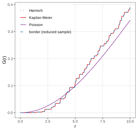
The empirical \(G\) lies below the Poisson curve for small distances (almost no neighbours closer than 2 units: cells have a size and do not overlap) and above it beyond the crossing at about \(r=4.2\) to \(5\) (the step function crosses the smooth curve several times there) (the book: "around 4.5"): more short-to-moderate nearest-neighbour distances than under CSR, a sign of clustering.
Algorithm 11.4 (Monte Carlo envelope test against CSR)
- Compute the summary \(\hat T(r)\) (\(\hat G\), \(\hat K\), \(\hat L\) or \(\hat g\)) of the data with \(n\) points.
- Simulate \(m\) patterns of \(n\) independent uniform points in \(W\) (Result 11.9) and compute \(\hat T_1,\dots,\hat T_m\) with the same estimator.
- Plot the pointwise envelope \(\min_j\hat T_j(r)\), \(\max_j\hat T_j(r)\).
Under CSR the data and the simulations are exchangeable, so at a fixed \(r\) fixed in advance, \(\Prob(\hat T(r)\) outside the envelope\()=2/(m+1)\): \(m=39\) gives a two-sided test of size 5%. Reading the envelope at many \(r\) at once inflates the size; a global test uses \(\max_r|\hat T(r)-T_{\mathrm{CSR}}(r)|\) ranked among the simulations.
11.17.1 Ripley's \(K\) function
Definition 11.8 (\(K\), \(L\) and \(g\) for a stationary isotropic process) Section 11.17.1, (11.11), (11.12)
\(\lambda K(r)\) is the expected number of further points within distance \(r\) of a typical point. Equivalently, for every \(B\) with \(|B|>0\),
\[ K(r)=\frac{1}{\lambda^2|B|}\,\E\sum_{x\in X\cap B}\ \sum_{y\in X,\,y\ne x}\ind\{|x-y|\le r\}. \]The \(L\) function is \(L(r)=\sqrt{K(r)/\pi}\) (11.11) and the pair correlation function is \(g(r)=K'(r)/(2\pi r)\) (11.12).
Result 11.11 (\(K\) under complete spatial randomness)
For a homogeneous Poisson process, \(K(r)=\pi r^2\), \(L(r)=r\) and \(g(r)=1\). For a general stationary process with second-order intensity \(\rho^{(2)}(u,v)=\rho(|u-v|)\),
\[ K(r)=\int_{b(0,r)}\frac{\rho(|h|)}{\lambda^2}\,\d h=2\pi\int_0^r g(t)\,t\,\d t,\qquad g(t)=\frac{\rho(t)}{\lambda^2}. \]Proof
Apply the second Campbell formula (Result 11.8) to \(h(u,v)=\ind_B(u)\ind\{|u-v|\le r\}\):
\[ \E\sum_{x\in B}\sum_{y\ne x}\ind\{|x-y|\le r\}=\int_B\int\ind\{|u-v|\le r\}\rho(|u-v|)\,\d v\,\d u=|B|\int_{b(0,r)}\rho(|h|)\,\d h. \]Dividing by \(\lambda^2|B|\) gives the first formula; polar coordinates (\(\d h=t\,\d t\,\d\phi\)) give the second, and differentiating it gives \(g(r)=K'(r)/(2\pi r)\), which is (11.12): the pair correlation is the normalised second-order intensity. For the Poisson process \(\rho\equiv\lambda^2\) (Result 11.9), so \(g\equiv1\) and \(K(r)=\pi r^2\); then \(L(r)=\sqrt{\pi r^2/\pi}=r\). The same answer follows from Slivnyak's theorem: given a point at \(u\), the others are Poisson, and the expected number within \(r\) is \(\lambda\pi r^2\). ∎
Interpretation: \(K(r)>\pi r^2\) (or \(g>1\), or \(L(r)>r\)) means more pairs at distance up to \(r\) than under CSR, clustering; below means inhibition (regularity).
Result 11.12 (edge-corrected estimators of \(K\) are unbiased)
For \(n\) points in a window \(W\) and \(d_{ij}=|x_i-x_j|\), consider
\[ \hat K(r)=\frac{|W|}{n(n-1)}\sum_{i\ne j}w_{ij}\,\ind\{d_{ij}\le r\} \]with the translation weight \(w_{ij}=|W|/|W\cap(W+x_i-x_j)|\) or Ripley's isotropic weight \(w_{ij}=2\pi d_{ij}/\ell_{ij}\), \(\ell_{ij}\) the length of the part of the circle of radius \(d_{ij}\) about \(x_i\) inside \(W\). With \(\lambda^2\) in place of \(n(n-1)/|W|^2\), both are unbiased for \(K(r)\) for a stationary (and, for Ripley's, isotropic) process; with \(n(n-1)/|W|^2\) they are exactly unbiased under CSR conditional on \(n\). Without weights (\(w_{ij}=1\)) the estimator is biased downwards.
Proof
By the second Campbell formula with stationarity, \(\rho^{(2)}(u,v)=\lambda^2g(u-v)\), and \(h(u,v)\)
substituting \(v=u-h\). For the translation weight \(w=|W|/|W\cap(W+h)|\) is constant in \(u\), and \(\int\ind_W(u)\ind_W(u-h)\,\d u=|W\cap(W+h)|\), so the bracket is \(|W|\) and the expectation is \(\lambda^2|W|K(r)\). For Ripley's weight, write \(h\) in polar form \((t,\phi)\) and use isotropy, \(g(h)=g(t)\): for fixed \(u\in W\) and \(t\), \(\int_0^{2\pi}\ind_W(u-t e_\phi)\,\d\phi=\ell(u,t)/t\) and \(w=2\pi t/\ell(u,t)\), so the angular integral of \(\ind_W\cdot w\) is \(2\pi\) and again the total is \(\lambda^2|W|\,2\pi\int_0^rg(t)t\,\d t=\lambda^2|W|K(r)\). Dividing by \(\lambda^2|W|\) proves unbiasedness. Under CSR given \(n\), the points are i.i.d. uniform (Result 11.9), each ordered pair has density \(|W|^{-2}\), and the same computation with \(n(n-1)\) pairs gives \(\E\hat K=K\) exactly. With \(w\equiv1\) the bracket is \(|W\cap(W+h)|<|W|\): pairs that straddle the boundary are missing. The border estimator \(\sum_{i:b_i\ge r}\sum_{j\ne i}\ind\{d_{ij}\le r\}/(\hat\lambda\,\#\{i:b_i\ge r\})\) is ratio-unbiased by the reduced-sample argument of Filling the gap 11.15. In 60 simulated CSR patterns, the border, isotropic and translation estimates averaged within 2% of \(\pi r^2\) at \(r=5,10,15\) (window side 100), the uncorrected one 6–14% below. ∎
Filling the gap 11.16: why \(L=\sqrt{K/\pi}\) "stabilises the variance" Section 11.17.1, after (11.11)
Derivation
Under CSR and for \(r\) small compared with the window, the pair count \(C(r)=\sum_{i\ne j}\ind\{d_{ij}\le r\}\) is twice a sum of many weakly dependent rare indicators, approximately \(2\times\) Poisson with mean \(\frac12n^2\pi r^2/|W|\). Then \(\hat K=|W|C/n^2\) has
\[ \E\hat K\approx\pi r^2=K,\qquad \var\hat K\approx\frac{|W|^2}{n^4}\cdot4\cdot\frac{n^2\pi r^2}{2|W|}=\frac{2|W|}{n^2}\,K(r)=\frac{2}{\lambda^2|W|}\,K(r): \]the variance is proportional to the mean, as for a Poisson count. The delta method for \(\phi(K)=\sqrt{K/\pi}\), \(\phi'(K)=1/(2\sqrt{\pi K})\), gives
\[ \var\hat L(r)\approx\phi'(K)^2\var\hat K=\frac{1}{4\pi K}\cdot\frac{2K}{\lambda^2|W|}=\frac{1}{2\pi\lambda^2|W|}=\frac{|W|}{2\pi n^2}, \]which does not depend on \(r\): the square root is the variance-stabilising transformation of a Poisson-like count (as in Chapter 8). This is the approximation of Ripley (1988) for small \(r\); for larger \(r\) edge effects and the dependence between pairs add terms, but \(\hat L(r)-r\) remains much more homogeneous in \(r\) than \(\hat K(r)-\pi r^2\), which is why plots and tests use \(L\). ∎
Result 11.13 (a clustered example: the Thomas process)
Let parents form a Poisson process of intensity \(\kappa\); each parent has a \(\Pois(\mu)\) number of offspring placed independently at \(\N(0,s^2\mathbf{I})\) displacements; the offspring form the process, with \(\lambda=\kappa\mu\). Then
\[ K(r)=\pi r^2+\frac{1}{\kappa}\big(1-e^{-r^2/(4s^2)}\big),\qquad g(r)=1+\frac{e^{-r^2/(4s^2)}}{4\pi\kappa s^2}. \]Proof
Pairs of offspring of different parents behave like a Poisson process (independent parents): their contribution to \(\rho^{(2)}\) is \(\lambda^2\). Pairs from the same parent: a parent contributes \(\E[M(M-1)]=\mu^2\) ordered pairs (for \(M\sim\Pois(\mu)\)), parents have intensity \(\kappa\), and the difference of two independent \(\N(0,s^2\mathbf I)\) displacements is \(\N(0,2s^2\mathbf I)\), with density \(e^{-|h|^2/(4s^2)}/(4\pi s^2)\). So \(\rho^{(2)}(h)\)
The excess \(K(r)-\pi r^2\) rises to \(1/\kappa\), the reciprocal parent intensity, over a range of a few \(s\): \(K\) reveals both the size and the scale of the clusters.
For an inhomogeneous process, clustering in \(K\) can simply reflect a varying intensity. Baddeley, Møller and Waagepetersen (2000) reweight each pair by the intensities at its two points:
\[ \hat K_{\inhom}(r)=\frac{1}{|W|}\sum_{i\ne j}\ind\{d(p_i,p_j)\le r\}\,\frac{e(p_i,p_j,r)}{\lambda(p_i)\,\lambda(p_j)}. \tag{11.10} \]Erratum (11.10)
The book's (11.10) omits the factor \(1/|W|\), runs the sum over all \(i,j\) (it must exclude \(i=j\), whose distance 0 would add \(\sum_i1/\lambda(p_i)^2\) to every \(K(r)\)), and writes the intensities as \(\lambda(x_i)\) for points named \(p_i\). The corrected form is displayed above; with these corrections it reduces to the homogeneous estimator of Result 11.12 when \(\lambda\) is constant.
Filling the gap 11.17: why the reweighted \(K\) works, and how \(\lambda\) is estimated (11.10), Figure 11.28
Derivation
Assumption. \(X\) is second-order intensity-reweighted stationary: \(\rho^{(2)}(u,v)=\lambda(u)\lambda(v)\,g(u-v)\) for a function \(g\) of the difference only. (An inhomogeneous Poisson process has \(g\equiv1\); thinning a stationary process with a location-dependent retention probability preserves this form.) Define \(K_{\inhom}(r)=\int_{b(0,r)}g(h)\,\d h\).
Unbiasedness. By the second Campbell formula with the border weight \(e=\ind\{b_i\ge r\}\) and the true \(\lambda\),
\[ \E\sum_{i\ne j}\frac{\ind\{b(x_i,r)\subseteq W\}\ind\{d_{ij}\le r\}}{\lambda(x_i)\lambda(x_j)}=\int_{W_{\ero r}}\int\ind\{|u-v|\le r\}\frac{\lambda(u)\lambda(v)g(u-v)}{\lambda(u)\lambda(v)}\,\d v\,\d u=|W_{\ero r}|\,K_{\inhom}(r). \]Dividing by \(|W_{\ero r}|\) gives the "modified border" estimator; dividing instead by \(\sum_i\ind\{b_i\ge r\}/\lambda(x_i)\), whose expectation is \(|W_{\ero r}|\) by the first Campbell formula, gives the "border" ratio estimator. Both are plotted in Figure 11.28. (On simulated inhomogeneous Poisson patterns with the true intensity both average to \(\pi r^2\) within 8%; the implementation agrees with a brute-force double sum to \(10^{-9}\).)
Estimating \(\lambda\). The intensity at the data points is estimated by a Gaussian kernel with bandwidth \(\sigma\approx1680\) (one eighth of the shorter side of the bounding rectangle), uniform edge correction, and leave-one-out (the point itself is excluded; otherwise each \(\hat\lambda(x_i)\) contains the spike \(K_\sigma(0)\) and \(\hat K\) is biased down). The estimates are then rescaled so that \(\sum_i1/\hat\lambda(x_i)=|W|\), the empirical version of the Campbell identity \(\E\sum_i1/\lambda(x_i)=|W|\). The level of \(\hat L_{\inhom}\) depends on these choices: with the 103,681 T cells, \(\hat\lambda\) is smooth on a scale of 1680 units while the T cells avoid tumour patches and lost tiles on smaller scales, so part of that structure remains as apparent "clustering". The book's spatstat defaults differ in details of the bandwidth and normalisation; its curves (\(\hat L\approx970\)–\(990\) at \(r=695\)) and mine (987 border, 1098 modified border) agree in shape and size of the effect, not to the last digit. ∎
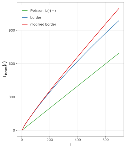
Setiadi et al. (2010) compared such curves between cell types and between tumour-draining and healthy lymph nodes, and found that B cells lose their normal arrangement in some tumours.
The pair correlation function
The pair correlation (11.12), \(g(r)=K'(r)/(2\pi r)\), is the density version of \(K\): \(\lambda g(r)\,\d A\) is the expected number of points in a small area \(\d A\) at distance \(r\) from a typical point, relative to \(\lambda\,\d A\) under CSR (Result 11.11). \(g=1\) for Poisson; \(g<1\) indicates inhibition and \(g>1\) clustering at that distance. Unlike \(K\), it is not cumulative, so effects at different scales do not mix.
Filling the gap 11.18: estimating \(g\) by differentiating \(\hat K\) (11.12), Figures 11.29, 11.30, Question 11.14
Derivation
\(\hat K\) is a step function, so (11.12) cannot be applied directly. Write \(K(r)=\pi r^2J(r)\); then \(K'(r)=2\pi rJ(r)+\pi r^2J'(r)\) and
\[ g(r)=J(r)+\frac r2J'(r),\qquad J(r)=\frac{K(r)}{\pi r^2}. \]\(J\) is bounded near 0 (it is a local average of \(g\)), so a smoothing spline through \(\hat J\) on the grid of \(r\) values, differentiated analytically, gives a stable \(\hat g\); differentiating a spline through \(\hat K\) itself is poorly behaved near \(r=0\), where \(\hat K\approx0\) but its derivative estimate leaks from larger \(r\). The result depends on the grid: on the default grid of 513 values with step \(1.36\) there are only 7 grid points in \([0,10]\) (Figure 11.29b); sampling \(r\) every 0.2 resolves the short-range structure (Figure 11.30), the answer to Question 11.14. An alternative is the kernel estimator \(\hat g(r)\)
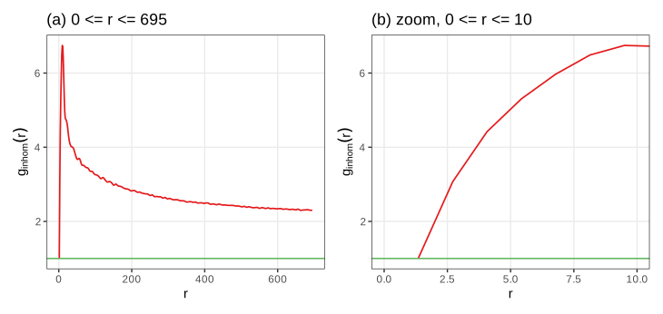
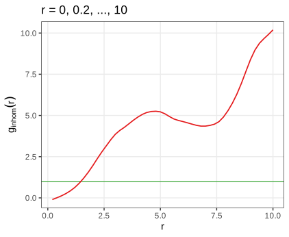
The T cells avoid each other below about 2 units (their own size: \(\hat K_{\inhom}(1.9)\) is only half of \(\pi\cdot1.9^2\), while \(\hat K_{\inhom}(5)\) is 3.9 times \(\pi\cdot5^2\)) and cluster strongly beyond, with \(\hat g\) decreasing slowly but still near 2 at 700 units, partly a trace of the inhomogeneity that the smooth \(\hat\lambda\) leaves in (Filling the gap 11.17).
Summary
- Images are arrays: pointwise maps change the histogram by a change of variables; geometric maps need inverse mapping and interpolation.
- Linear shift-equivariant filters are convolutions, computed by the FFT; Gaussian smoothing trades a variance reduction \(\approx1/(4\pi\sigma^2)\) against a bias \(\frac{\sigma^2}2\Delta f\).
- Adaptive thresholds work when objects are sparse relative to the averaging disc; morphological operations are Minkowski set operations with a clean algebra (duality, idempotent opening and closing).
- Objects are connected components; Voronoi propagation on the image surface, computed by Dijkstra's algorithm, grows seeds into cells with \(\lambda\) controlling geometry against signal.
- Cell positions are point patterns. CSR gives \(G=1-e^{-\lambda\pi r^2}\), \(K=\pi r^2\), \(L=r\), \(g=1\); edge-corrected estimators are unbiased by the Campbell–Mecke formula; \(L\) stabilises the variance; reweighting by \(\lambda\) separates interaction from inhomogeneity.
Questions in the text
Short answers to the questions the book asks along the way (its Questions 11.1 to 11.14).
- Formats beyond JPEG, PNG and TIFF. The RBioFormats package interfaces the Bio-Formats library of the Open Microscopy Environment, which reads well over a hundred (mostly proprietary microscopy) formats; its documentation keeps the current list.
- Why display
1 - nuc? The nuclei are bright on a black background; \(1-f\) shows them dark on white, which prints better. Displayingnucdirectly gives white nuclei on black. - Slots and methods.
showClass("Image")lists the slots (.Data,colormode);showMethods(classes = "Image")lists the methods defined for the class. - How is
nucstored? As a \(510\times510\times4\) array of doubles withcolorModeGrayscale, so the third dimension holds 4 frames. - Memory.
hivctakes 29.8 MB, 8 bytes per value; the JPEG at quality 85 about 0.3 MB; a 16-megapixel three-channel image 384 MB (Section 11.5). - What does
normalizedo? It maps the range of the values linearly onto \([0,1]\) (by default, each frame separately): \(f\mapsto(f-\min f)/(\max f-\min f)\); with \(-f\) this inverts the image (checked to machine precision). - Type of
mosqthresh. AnImagewhose array has storage mode logical. tortranspose? They agree for a single grey-scale frame;transposeswaps only the two spatial dimensions and so also works for colour images and stacks, wheretfails.- What does the weight matrix look like? A discretised bivariate normal density (Figure 11.10, Filling the gap 11.5).
- The numbers in
table(nucSeed). The areas, in pixels, of the background (label 0) and of the 43 objects. - Selecting a partition element.
voronoiExampis an integer image;which(voronoiExamp == 13, arr.ind = TRUE)returns the pixel coordinates of cell 13. With the current EBImage the first three cell areas are 5648, 4735 and 373 pixels (the book prints 5645, 4735, 370, from an earlier run). - Why are the \(y\) axes of Figures 11.20 and 11.21 inverted relative to each other? Images put the origin at the top left with \(y\) downwards; Cartesian plots at the bottom left with \(y\) upwards.
- The intensity without edge correction. Figure 11.25: lower near the boundary, by the factor \(e_W(p)\) (Filling the gap 11.13).
- Increasing the resolution of \(\hat g\). Pass a finer grid
rto the estimator of \(K\) (Figure 11.30, Filling the gap 11.18).
Exercises
The six exercises of Chapter 11, restated in my own words, with worked solutions (hidden).
Exercise 11.1. Read a few of your own photographs into R and apply the manipulations of Section 11.6 to them.
Solution
x = readImage("photo.jpg")gives a \(w\times h\times3\) Color image with values on the 8-bit grid.x^(1/3),x * 3andnormalize(-x)act channel by channel; by Filling the gap 11.2, the gamma map spreads the dark tones, the multiplication saturates every value above \(1/3\), and inversion reflects each channel's histogram (a colour negative). Applying a power to a colour photo changes hues slightly, because the three channels are transformed by the same non-linear map of different values; converting to grey first (channel(x, "gray")) avoids that. Rotations need interpolation and enlarge the canvas (Filling the gap 11.3);flip,flopandtransposeare exact.Exercise 11.2. Explore the effect of
lambdainpropagate(Sections 11.12, 11.13) with an interactive display of the cell-body segmentation.Solution
This is the Voronoi propagation demonstration, which recomputes the segmentation in the browser for any \(\lambda\) and reproduces
propagate(cell areas 2010, 1334, 372, ... at \(\lambda=0.01\), the same as R). Observations: for \(\lambda\ge10\) the cell boundaries are nearly the Voronoi bisectors cut by the mask, whatever the actin signal does; as \(\lambda\) decreases, boundaries move into the dark valleys of the actin stain, which is right where cells touch but can produce irregular, elongated cells where the signal is flat or noisy; for \(\lambda\le10^{-4}\) regions spread along plateaus. Because the step cost is \(\sqrt{(\d z^2+\lambda|\d p|^2)/(1+\lambda)}\), \(\lambda\) is the squared intensity difference that costs as much as one pixel of lateral movement: \(\lambda=0.01\) equates one pixel with a summed 3 × 3 intensity change of 0.1, a sensible scale for the actin values (about 0.03 to 0.9).Exercise 11.3. For an image \(B\) on the pixel set \(I\), the empirical autocorrelation is
\[ a(v_x,v_y)=\frac1{|I|}\sum_{(x,y)\in I}B(x,y)\,B(x+v_x,\,y+v_y). \tag{11.13} \]The book's function
autocorr2dcomputes it by the Wiener–Khinchin theorem with the FFT, after dividing the image by its sum, and shifts the zero lag to the centre. Apply it to the three channels ofcells(Figure 11.31), average over the angle (Figure 11.32), and answer: how would you compute cross-correlations between channels; why the sum normalisation; should the mean be subtracted first; how does this relate tovarandcor; how could such curves serve as quality metrics in a screen; and what would a 3- or \(n\)-dimensional version be good for?Solution
Wiener–Khinchin. With circular lags, \(a(v)=|I|^{-1}\sum_pB(p)B(p+v)\). Its DFT is \(|I|^{-1}\sum_v\sum_pB(p)B(p+v)e^{-2\pi i\langle k,v\rangle}\)
\({}=|I|^{-1}\overline{\DFT B(k)}\,\DFT B(k)\) \({}=|I|^{-1}|\DFT B(k)|^2\) (substitute \(q=p+v\)), so \(a=|I|^{-1}\DFT^{-1}|\DFT B|^2\): the autocorrelation is the inverse transform of the power spectrum. R's fft(..., inverse = TRUE)omits the factor \(1/|I|\); with \(b=B/\sum B\) the book's function therefore returns \(\sum_pb(p)b(p+v)\cdot|I|=a(v)/\bar B^2\), \(\bar B\) the mean (checked against the direct sum to \(10^{-16}\)). The lags are circular: the image is treated as a torus, so large lags mix opposite edges.Sum normalisation. Dividing by \(\bar B^2\) makes the curve independent of the overall brightness and exposure, so channels and images can be compared: the value at lag 0 is \(\overline{B^2}/\bar B^2=1+\mathrm{CV}^2\), and at large lags (no correlation) it tends to 1.
Subtracting the mean first gives the autocovariance \(c(v)\)
\({}=|I|^{-1}\sum_p(B(p)-\bar B)(B(p+v)-\bar B)\) \({}=a(v)-\bar B^2\); dividing by \(c(0)\) gives the autocorrelation in the statistical sense, \(\rho(v)=c(v)/c(0)\in[-1,1]\), with \(\rho(0)=1\) and decay to 0. It removes the constant baseline that dominates \(a\) and is usually preferable. Relation to var and cor. \(c(0)\) is the population variance of the pixel values (
vartimes \((|I|-1)/|I|\)), and \(\rho(v)\) is (up to the circular wrap) the correlation (cor) between the image and its copy shifted by \(v\).Cross-correlation of channels \(B_1,B_2\): replace \(|\DFT B|^2\) by \(\overline{\DFT B_1}\,\DFT B_2\); its peak location estimates the shift between channels (registration) and its height their co-localisation.
Quality metrics. The radial profile has a characteristic width (the correlation length: nuclear size for DAPI, larger for the cytoplasmic stains, Figure 11.32). Out-of-focus images have wider profiles, saturated or empty images abnormal values at lag 0, and debris or illumination artefacts long tails; summarising each image by a few profile features (value at lag 0, lag where \(\rho\) drops to \(\frac12\)) and flagging outliers is a cheap automatic quality control for millions of images.
Higher dimensions. The same formula with an \(n\)-dimensional FFT gives spatial autocorrelation of 3D stacks (anisotropy between \(z\) and \(x,y\) reveals the point-spread function) or spatio-temporal autocorrelation of movies (a time lag measures how fast structures change).
A detail. The book measures the radius from \((n_1/2,n_2/2)=(170,245)\), but after
fftshifton even dimensions the zero lag sits at \((n_1/2+1,n_2/2+1)=(171,246)\), where the book's radius is 1. Figures 11.31 and 11.32 here use the corrected centre; the effect is a shift of the profile by up to one pixel.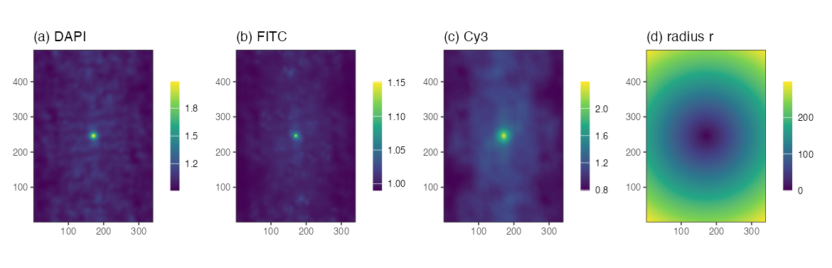
Figure 11.31. Autocorrelation \(a(v)/\bar B^2\) of the DAPI, FITC and Cy3 channels, zero lag in the centre, and the radius \(r\) measured from the zero lag. Reproduces Holmes and Huber (2019), Figure 11.31. Download: PDF 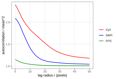
Figure 11.32. The autocorrelations of Figure 11.31 averaged over the angle, for \(r\le50\): the DNA signal decorrelates over a few pixels (small nuclei), the actin over tens of pixels. Reproduces Holmes and Huber (2019), Figure 11.32. Download: PDF · SVG Exercise 11.4. The book points to further tutorial material with other images (more segmentation, and optical flow). As a self-contained substitute: apply the nuclear pipeline of Algorithm 11.2 to the four frames of
nuclei.tif(Figure 11.3) and compare it with a global threshold.Solution
The frames are 8-bit-like images with values up to about 1, so the offset is raised to 0.05. Smoothing with \(\sigma=1\), the adaptive threshold (disc 21, offset 0.05) and an opening with the disc of diameter 5 give 77, 86, 94 and 90 objects in frames 1 to 4. A global threshold chosen by Otsu's method (maximising the between-class variance of the grey-level histogram; thresholds 0.34 to 0.40) gives 69, 72, 77 and 74. The adaptive threshold finds more objects because it also splits touching nuclei (the local mean rises between them, Filling the gap 11.7); it also keeps a few small fragments, which a size filter on the object areas (Question 11.10) would remove. Without manual annotation neither count is "true": in practice one checks a sample of objects by eye, the point the book makes about ground truth in Section 11.11.
Exercise 11.5. Compute and display the Voronoi tessellation of the Ukrainian cities of Chapter 9, either from their MDS coordinates in the plane or from latitude and longitude with the great-circle (haversine) distance.
Solution
Plane. Classical MDS of the 33 × 33 distance matrix (
cmdscale) gives coordinates in kilometres;deldircomputes the Voronoi tiles inside a box 10% larger than the points. The largest tiles belong to cities on the edge of the point cloud, where the box, not another city, bounds the tile: Uzhhorod (about 112,000 km²), Chernivtsi (100,000), Simferopol (77,000), Lutsk (76,000); tiles of the edge cities are artefacts of the box.Sphere. The haversine distance
\[ d=2R\arcsin\sqrt{\sin^2\frac{\Delta\varphi}2+\cos\varphi_1\cos\varphi_2\sin^2\frac{\Delta\lambda}2} \](\(R=6371\) km, \(\varphi\) latitude, \(\lambda\) longitude) assigns each point of a 0.05° grid to its nearest city. To compare, rotate (or reflect) the MDS map onto a local projection of the coordinates by orthogonal Procrustes analysis (SVD of the cross-product matrix): the residual is only 12 km per city, so MDS recovers the map up to a rigid motion, and the nearest city in the aligned MDS plane agrees with the great-circle nearest city on 89% of the area. The disagreements lie along the tile boundaries, where small distortions of the planar map (the matrix is of road or great-circle distances, not planar ones) move the bisectors.
Exercise 11.6. Download three-dimensional light-sheet microscopy data, read it into an EBImage
Imageand explore it.Solution (method)
A z-stack read with
readImagebecomes a GrayscaleImageof dimension \(n_x\times n_y\times n_z\), the third dimension being frames. Points to watch: (i) memory: \(2048\times2048\times1000\) voxels as doubles take 33.6 GB, so read sub-volumes or keep integer storage; (ii) voxels are usually anisotropic (\(z\) spacing several times the \(x,y\) spacing), so smoothing kernels and distances must be scaled per axis; (iii) the 2D tools generalise: a separable 3D Gaussian is three 1D convolutions; 3D morphology uses a ball as structuring element; connected components use 6- or 26-adjacency (paired as in Filling the gap 11.8); maximum-intensity projections along \(z\) give quick 2D overviews; and the autocorrelation of Exercise 11.3 in 3D measures the anisotropy of the point-spread function.
Demonstrations for this chapter
Each demonstration runs in the browser on data exported by the R code, and reproduces the R numbers. The ▶ Demo boxes above open them already set to the case under discussion.
| Demonstration | What you can see | Sections and results |
|---|---|---|
| Segmenting nuclei: smoothing, adaptive thresholding and morphology | The DNA channel of the HCT116 cells: Gaussian smoothing, global or adaptive threshold, simulated uneven illumination, erosion, dilation, opening, closing, labelling. Presets: 1 the book's pipeline, 43 nuclei; 2 uneven illumination, global threshold; 3 uneven illumination, adaptive threshold; 4 offset too small; 5 what the opening removes. | 11.8.2, 11.9 (Gap 11.7), 11.10 (Result 11.4), 11.11 |
| Voronoi tessellation on an image manifold: segmenting cell bodies | Dijkstra propagation of the 43 nuclei over the actin landscape for any λ, with or without the cytoplasm mask, flat or actin landscape, window or pixel increment; click a cell for its area. Presets: 1 the book's cell bodies; 2 plain Voronoi; 3 λ = 100; 4 λ = 0.0001; 5 single-pixel increment. | 11.12 (Gap 11.9, Algorithm 11.3, Result 11.6), 11.13 |
| Spatial point patterns: Ripley's K, L, the pair correlation and G | T cells, tumour cells and other cells in a window of the lymph node, CSR, Thomas and hard-core simulations; K, L − r, g, G with four edge corrections, CSR envelopes, kernel intensity with three edge treatments. Presets: 1 CSR; 2 Thomas clusters; 3 hard core; 4 T cells; 5 edge effects. | 11.16.1, 11.16.2 (Gap 11.13), 11.17 (Algorithm 11.4), 11.17.1 (Results 11.11–11.13) |
The R code for every figure of this page is code/ch11_image_data.R (see the code index).
References
- Holmes, S. and Huber, W. (2019). Modern Statistics for Modern Biology. Cambridge University Press. Chapter 11.
- Andrew, A. M. (1979). Another efficient algorithm for convex hulls in two dimensions. Information Processing Letters, 9(5), 216–219. doi:10.1016/0020-0190(79)90072-3.
- Baddeley, A. J. and Gill, R. D. (1997). Kaplan–Meier estimators of distance distributions for spatial point processes. The Annals of Statistics, 25(1), 263–292. doi:10.1214/aos/1034276629.
- Baddeley, A. J., Møller, J. and Waagepetersen, R. (2000). Non- and semi-parametric estimation of interaction in inhomogeneous point patterns. Statistica Neerlandica, 54(3), 329–350. doi:10.1111/1467-9574.00144.
- Bickel, D. R. (2002). Robust estimators of the mode and skewness of continuous data. Computational Statistics & Data Analysis, 39(2), 153–163. doi:10.1016/S0167-9473(01)00057-3.
- Chiu, S. N., Stoyan, D., Kendall, W. S. and Mecke, J. (2013). Stochastic Geometry and Its Applications, 3rd edition. Wiley.
- Diggle, P. J. (1985). A kernel method for smoothing point process data. Applied Statistics, 34(2), 138–147. doi:10.2307/2347366.
- Diggle, P. J. (2013). Statistical Analysis of Spatial and Spatio-Temporal Point Patterns, 3rd edition. Chapman and Hall/CRC.
- Dijkstra, E. W. (1959). A note on two problems in connexion with graphs. Numerische Mathematik, 1, 269–271. doi:10.1007/BF01386390.
- Holmes, S., Kapelner, A. and Lee, P. P. (2009). An interactive Java statistical image segmentation system: GemIdent. Journal of Statistical Software, 30(10). doi:10.18637/jss.v030.i10.
- Jones, T. R., Carpenter, A. and Golland, P. (2005). Voronoi-based segmentation of cells on image manifolds. In Computer Vision for Biomedical Image Applications, Lecture Notes in Computer Science 3765, 535–543. doi:10.1007/11569541_54.
- Laufer, C., Fischer, B., Billmann, M., Huber, W. and Boutros, M. (2013). Mapping genetic interactions in human cancer cells with RNAi and multiparametric phenotyping. Nature Methods, 10, 427–431. doi:10.1038/nmeth.2436.
- Pau, G., Fuchs, F., Sklyar, O., Boutros, M. and Huber, W. (2010). EBImage: an R package for image processing with applications to cellular phenotypes. Bioinformatics, 26(7), 979–981. doi:10.1093/bioinformatics/btq046.
- Ripley, B. D. (1976). The second-order analysis of stationary point processes. Journal of Applied Probability, 13(2), 255–266. doi:10.2307/3212829.
- Ripley, B. D. (1988). Statistical Inference for Spatial Processes. Cambridge University Press.
- Rosenfeld, A. (1970). Connectivity in digital pictures. Journal of the ACM, 17(1), 146–160. doi:10.1145/321556.321570.
- Serra, J. (1983). Image Analysis and Mathematical Morphology. Academic Press.
- Setiadi, A. F., Ray, N. C., Kohrt, H. E., et al. (2010). Quantitative, architectural analysis of immune cell subsets in tumor-draining lymph nodes from breast cancer patients and healthy lymph nodes. PLoS One, 5(8), e12420. doi:10.1371/journal.pone.0012420.
- Shannon, C. E. (1948). A mathematical theory of communication. Bell System Technical Journal, 27(3), 379–423. doi:10.1002/j.1538-7305.1948.tb01338.x.
- Thomas, M. (1949). A generalization of Poisson's binomial limit for use in ecology. Biometrika, 36(1/2), 18–25. doi:10.2307/2332526.
- Vetterli, M., Kovačević, J. and Goyal, V. K. (2014). Foundations of Signal Processing. Cambridge University Press.
DOIs were checked against Crossref. The numerical statements in the text (pixel counts, agreement with EBImage, simulation results, the lymph-node summaries) come from the course R code; the figures from code/ch11_image_data.R.