Model Selection and Approximation in High-dimensional Mixtures of Experts Models: From Theory to Practice

TrungTin Nguyen

Chapter 1 · Introduction

1.1 Mixture of experts modelling framework

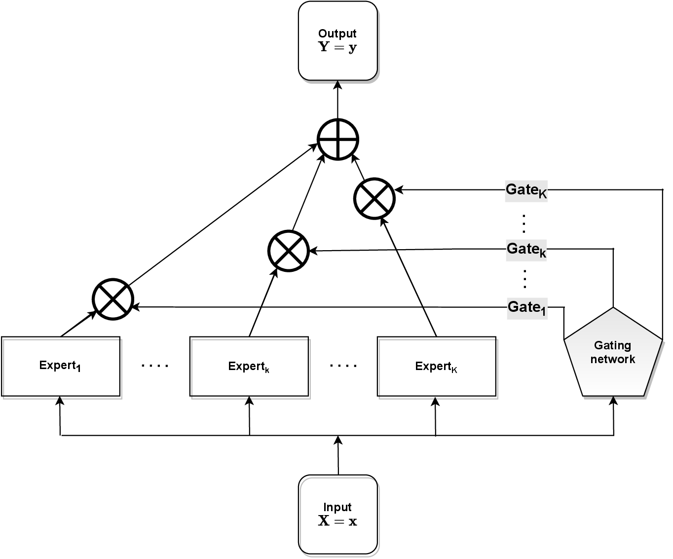
Mixture of experts (MoE) models, originally introduced as neural networks (NNs) in Jacobs et al., (1991) and Jordan and Jacobs, (1994), where they were used to model complex and heterogeneous data generating processes (DGPs). The main idea of MoE is a divide-and-conquer principle that proposes dividing a complex problem into a set of simpler subproblems and then one or more specialized problem-solving tools, or experts, are assigned to each of the subproblems. A schematic diagram of an MoE model as a NN is provided in Figure 1.1.

MoE are flexible models that generalize the classical finite mixture models as well as finite mixtures of regression models (McLachlan and Peel, 2000, Section 5.13), and are widely used in statistics and machine learning, thanks to their flexibility and the abundance of applicable statistical estimation and model selection tools. Their flexibility comes from allowing the mixture weights (or the gating functions, gating networks) to depend on the explanatory variables, along with the component densities (or experts). This permits the modeling of data arising from more complex data generating processes than the classical finite mixtures and finite mixtures of regression models, whose mixing parameters are independent of the covariates. Due to their flexibility, MoE can be used in many statistical problems, namely to cluster or classify data, to estimate conditional densities, to conduct regression analysis and to analyze regression outcomes. Detailed reviews on practical and theoretical aspects of MoE models can be found in Yuksel et al., (2012); Masoudnia and Ebrahimpour, (2014) and Nguyen and Chamroukhi, (2018).

Refer to caption — Figure 1.1: Schematic diagram of the NN architecture of a $K$ -component MoE model.

Statistically, we consider a regression framework and aim at capturing the potential nonlinear relationship between a multivariate response $𝐘$ and a vector of covariates $𝐗$ . Here and subsequently, $(𝐗_{[n]}, 𝐘_{[n]}) : = (𝐗_{i}, 𝐘_{i})_{i \in [n]}$ , $[n] = {1, \dots, n}, n \in ℕ^{⋆}$ , denotes a random sample, and $𝐱$ and $𝐲$ stands for the observed values of the random variables $𝐗$ and $𝐘$ , respectively. We assume that the response variable $𝐘$ depends on the explanatory variable $𝐗$ through a regression-type model. The explanatory variable goes by different names, such as covariate, predictor, independent variable, feature, or sometimes just variable. The response variable is often called the output or dependent variable. Throughout this thesis, we will use all of these terms interchangeably.

Firstly, we focus on a natural starting point for setting up a more probabilistic MoE model, often called “direct application” of mixture modelling; see Titterington et al., 1985 for more details. Then, we will specify an alternative perspective on mixture modelling in Sections 1.1.1 and 1.1.2 that provide an “analytic” view, complementary to this “synthetic” or “generative” view. Regarding the former perspective, suppose that the population from which we are sampling is heterogeneous, i.e., given an input $𝐗 = 𝐱$ , there are multiple groups (that can be interpreted as clusters), indexed by $k \in [K]$ , present in the population in proportions $g_{k} (𝐱; 𝝎), k \in [K]$ , where $𝝎$ is some parameter vector parametrising the input-dependent proportions function $g_{k} (𝐱; \cdot)$ , with $g_{k} (𝐱; 𝝎) > 0$ , and $\sum_{k = 1}^{K} g_{k} (𝐱; 𝝎) = 1$ . In this way, there is a latent unobserved random variable representation of the mixture model (usually called latent or allocation variables), involving the latent cluster membership of each observation, denoted by $Z \in [K], K \in ℕ^{⋆}$ , where $Z = k$ if observation $𝐲$ given the input $𝐱$ belongs to cluster $k$ for $k \in [K]$ . Next, the conditional relationship between $Z$ and the input $𝐗$ can be characterized by

p (Z = k | 𝐗 = 𝐱) = g_{k} (𝐱; 𝝎) .

(1.1.1)

Then, we can characterize the relationship between the output $𝐲$ and the input $𝐗$ by

p (𝐲 | 𝐗 = 𝐱, Z = k) = ϕ_{k} (𝐲; 𝜽_{k} (𝐱)),

(1.1.2)

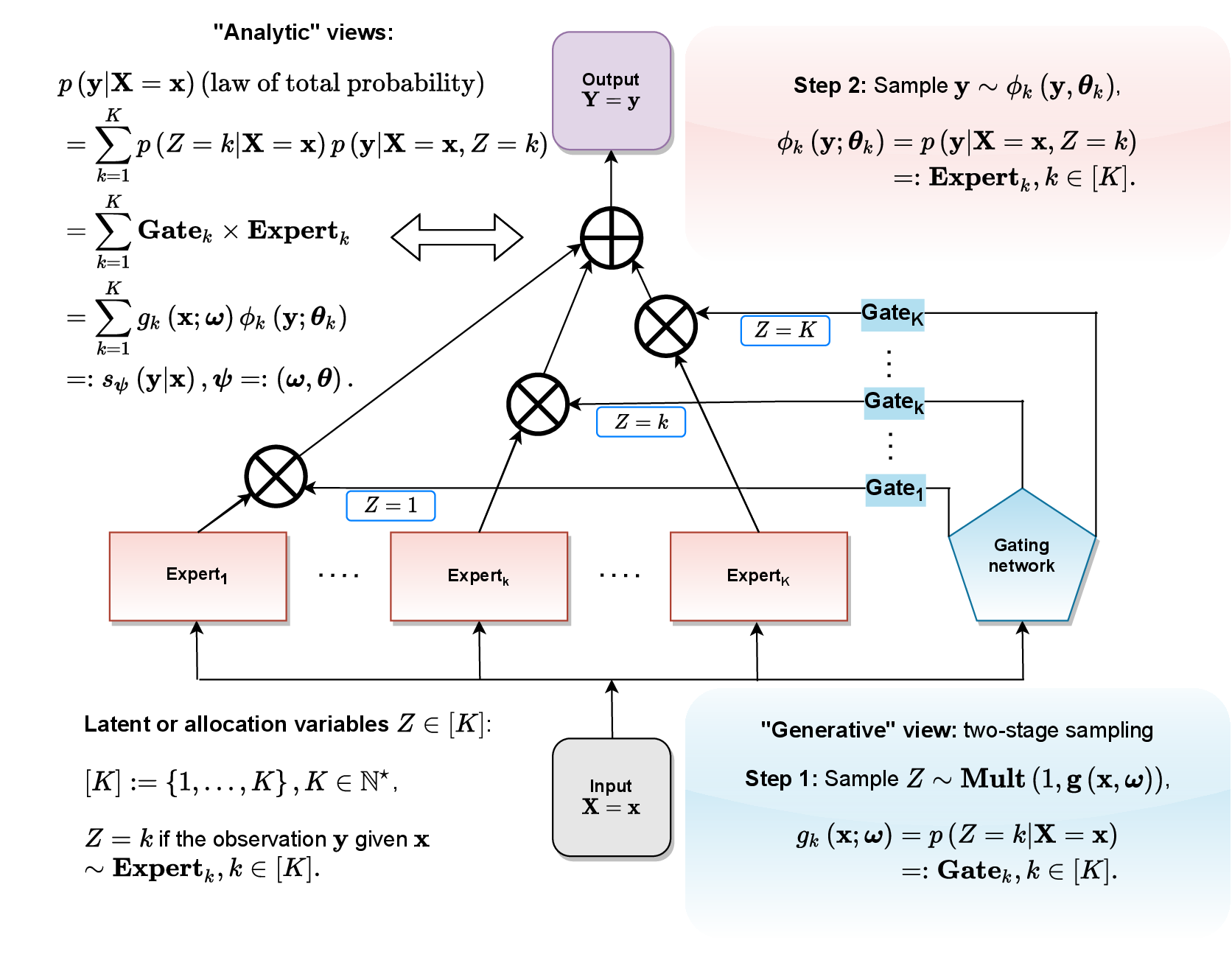
where $𝜽_{k} (𝐱)$ is some parameter vector and, given an input $𝐱$ , $ϕ_{k} (\cdot; 𝜽_{k} (𝐱))$ is a probability density function (PDF). We can imagine that given an input $𝐗 = 𝐱$ , the observed output $𝐲$ , drawn from the population, is generated in two step: firstly, the group $Z$ is drawn from a multinomial distribution with a single trial and probabilities equal to $𝐠 (𝐱; 𝝎) = (g_{k} (𝐱; 𝝎))_{k \in [K]}$ ; and secondly, given $𝐗 = 𝐱, Z = k$ , the output $𝐲$ is drawn from $ϕ_{k} (𝐲; 𝜽_{k} (𝐱))$ .

Note that this two-stage sampling gives exactly the same models in analytic views, see (1.1.4) and (1.1.17) for more details, for the conditional distribution of $𝐲 | 𝐱$ . Indeed, via characterizations (1.1.1) and (1.1.2), and by using the law of total probability, we can characterize the marginal relationship between the response and the input, unconditional on $Z$ , via the expression

	$p (𝐲 \| 𝐗 = 𝐱)$	$= \sum_{k = 1}^{K} p (𝐲 \| 𝐗 = 𝐱, Z = k) p (Z = k \| 𝐗 = 𝐱)$
		$= \sum_{k = 1}^{K} g_{k} (𝐱; 𝝎) ϕ_{k} (𝐲; 𝜽_{k} (𝐱)) = : s_{𝝍} (𝐲 \| 𝐱),$		(1.1.3)

where $𝝍 = (𝝎, 𝜽)$ is the vector of all parameter elements that are required in characterizing (1.1), see Figure 1.2 for more details.

For a better comparison between a standard MoE regression model (in which all model parameters are functions of covariates) and the special cases, where some of the model parameters do not depend on covariates, the four models in the MoE framework are presented in Figure 1.3; see also Fruhwirth-Schnatter et al., (2019, Chapter 12) for more detail.

(a) Mixture model

(b) MoE regression model

(c) Simple MoE regression model

(d) Standard MoE regression model

Figure 1.3: Based on the graphical model representation, namely the presence or absence of edges between the covariates

𝐱

and the latent variable

Z

and response variable

𝐲

, there are four special cases of MoE regression models. More precisely, in Figure 1.3(a),

p (𝐲, Z | 𝐱) = p (𝐲 | Z) p (Z)

; in Figure 1.3(b),

p (𝐲, Z | 𝐱) = p (𝐲 | 𝐱, Z) p (Z)

; in Figure 1.3(c),

p (𝐲, Z | 𝐱) = p (𝐲 | Z) p (Z | 𝐱)

; and in Figure 1.3(d),

p (𝐲, Z | 𝐱) = p (𝐲 | 𝐱, Z) p (Z | 𝐱)

. This figure is inspired from Fruhwirth-Schnatter et al., (2019, Chapter 12, Fig. 12.2).

In the context of regression, MoE models with Gaussian experts and softmax or Gaussian gating functions are the most popular choices and are powerful tools for modeling more complex non-linear relationships between responses and predictors that arise from different subpopulations. This is largely studied because of their universal approximation properties, see LABEL:chapter_ApproximationMoEs for more details, which have been extensively studied for not only finite mixture models (Genovese and Wasserman, 2000; Rakhlin et al., 2005; Nguyen, 2013; Ho et al., 2016a, ; Ho et al., 2016b, ; Nguyen et al., 2020d, ; Nguyen et al., 2020b, ) but also conditional densities of MoE models (Jiang and Tanner, 1999a, ; Norets et al., 2010; Nguyen et al., 2016; Ho et al., 2019; Nguyen et al., 2019; Nguyen et al., 2021a, ).

More precisely, LABEL:chapter_ApproximationMoEs (see also Section 1.4) provides a detailed exposition of these universal approximation properties. In particular, we prove that, to an arbitrary degree of accuracy, location-scale mixtures of a continuous PDF can approximate any continuous PDF, uniformly, on a compact set; and for any finite $p \geq 1$ , location-scale mixtures of an essentially-bounded PDF can approximate any PDF, in the $L_{p}$ norm. Moreover, given input and output variables that are both compactly supported, we demonstrate the richness of the class of MoE models by proving denseness results in Lebesgue spaces for conditional PDFs.

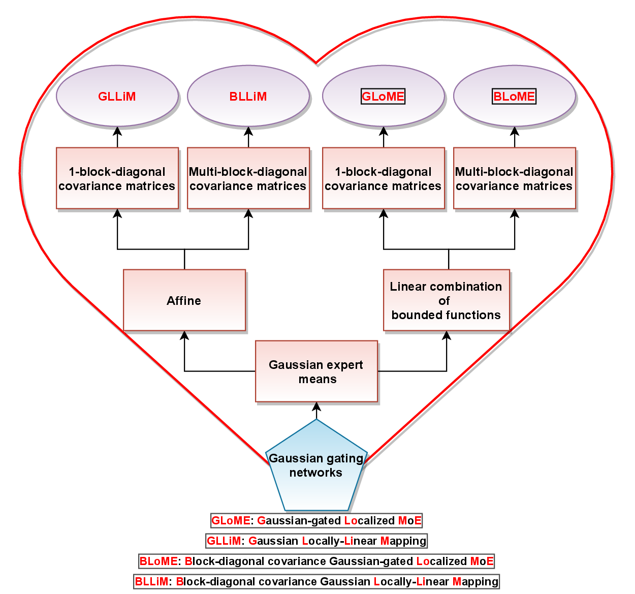
In this thesis, we wish to firstly investigate MoE models with Gaussian gating functions for clustering and regression, first introduced by Xu et al., (1995), which extended the original MoE models of Jacobs et al., (1991). Based on the works of Nguyen et al., 2021c ; Nguyen et al., 2021b , we refer to these models as Gaussian-gated localized MoE (GLoME) models and block-diagonal covariance for localized mixture of experts (BLoME) models, to be developed in LABEL:chapter_ModelSelectionMoEs. It is worth pointing out that the BLoME models generalize GLoME models by utilizing a parsimonious covariance structure, via block-diagonal structures for covariance matrices in the Gaussian experts. It is also interesting to point out that supervised Gaussian locally-linear mapping (GLLiM) and block-diagonal covariance for Gaussian locally-linear mapping (BLLiM) models in Deleforge et al., 2015c and Devijver et al., (2017) are affine instances of GLoME and BLoME models, respectively, where linear combination of bounded functions are considered instead of affine for mean functions of Gaussian experts.

Next, LABEL:chapter_JointRankVariableMoEs is devoted to the study of MoE models with softmax gating functions based on the idea of the original MoE models of Jacobs et al., (1991). In LABEL:chapter_JointRankVariableMoEs, we obtain what will be referred to as linear-combination-of-bounded-functions softmax-gated block-diagonal mixture of experts (LinBoSGaBloME) regression models. In particular, we simply refer to affine instances of LinBoSGaBloME models as softmax-gated mixture of experts (SGaME) regression models. One of the main drawbacks of LinBoSGaBloME models is the difficulty of applying an EM algorithm, which requires an internal iterative numerical optimization procedure (e.g., MM algorithm, iteratively-reweighted least squares, proximal Newton-type procedure, Newton-Raphson algorithm) to update the softmax parameters. GLoME and BLoME models overcome this problem by using the Gaussian gating network that enables us to link GLoME with finite mixtures of Gaussian models. Given its mixture model foundation, the maximization with respect to the parameters of the gating network can be solved analytically within the EM algorithm framework, which decreases the computational complexity of the estimation routine. Furthermore, we then can also make use of well established theoretical results for finite mixture models.

In spite of the fact that the MoE nomenclature has its origins in the machine learning literature (Jacobs et al., 1991), SGaME models have been broadly applied to numerous areas of science, technology and business, for the tasks of classification, clustering, and regression: switching regression models (Quandt, 1972), concomitant variable latent class models (Dayton and Macready, 1988), latent class regression models (DeSarbo and Cron, 1988), mixed models (Wang et al., 1996), functional data analysis and signal processing (Chamroukhi et al., 2009; Samé et al., 2011; Chamroukhi et al., 2013a, ), finite smooth mixtures (Li et al., 2011), image classification and semantic segmentation tasks (Wang et al., 2020), modeling neural connectivity Bock and Fine, (2014), segmentation of spectral images (Cohen and Le Pennec, 2014), climatic change modeling (Nguyen and McLachlan, 2014), phone activity recognition (Lee and Cho, 2014), heterogeneity modeling in neural connectivity data (Eavani et al., 2016), reinforcement learning (He et al., 2016), the tasks of language modeling and machine translation (Shazeer et al., 2017), multi-modal deep generative models on different sets of modalities including a challenging image-language dataset (Shi et al., 2019), anomaly detection (Yu et al., 2021), just to name a few.

The important point to note here is that both GLoME and BLoME models have been also thoroughly studied in the statistics and machine learning literatures and their forms appear in many different guises, including localized MoE (Ramamurti and Ghosh, 1996, 1998; Moerland, 1999; Bouchard, 2003), normalized Gaussian networks (Sato and Ishii, 2000), MoE modeling of priors in Bayesian nonparametric regression (Norets and Pelenis, 2014; Norets and Pati, 2017), cluster-weighted modeling (Ingrassia et al., 2012), GLLiM in inverse regression (Deleforge et al., 2015c, ), BLLiM model (Devijver et al., 2017), deep mixture of linear inverse regressions (Lathuilière et al., 2017), hierarchical Gaussian locally linear mapping structured mixture (HGLLiM) model (Tu et al., 2019), multiple-output Gaussian gated mixture of linear experts (Nguyen et al., 2019), and approximate Bayesian computation with surrogate posteriors using GLLiM (Forbes et al., 2021).

From now on, we are interested in estimating the law of the random variable $𝐘$ conditionally on $𝐗$ . The following assumptions will be needed throughout the chapter. We assume that the covariates $𝐗$ are independent but not necessarily identically distributed. The assumptions on the responses $𝐘$ are stronger: conditional on $𝐗_{[n]}$ , the $𝐘_{i}, i \in [n]$ , are independent, and each $𝐘$ follows a law with true (but unknown) PDF $s_{0} (\cdot | 𝐗 = 𝐱)$ , which is approximated via MoE models.

1.1.1 GLoME and BLoME models

Motivated by an inverse regression framework where the role of predictor and response variables should be exchanged such that $𝐘 = (𝐘_{j})_{j \in [L]}, [L] = {1, \dots, L}$ , becomes the input and $𝐗 = (𝐗_{j})_{j \in [D]}$ plays the role of a multivariate output, we consider the following GLoME model, defined by (1.1.4) (see also in Nguyen et al., 2021c, ). This construction goes back to the work of Li, (1991); Deleforge et al., 2015c , and Perthame et al., (2018). In this way, we define its corresponding conditional PDF as follows:

	$s_{𝝍_{K, d}} (𝐱 \| 𝐲)$	$= \sum_{k = 1}^{K} g_{k} (𝐲; 𝝎) ϕ_{D} (𝐱; 𝝊_{k, d} (𝐲), 𝚺_{k}),$		(1.1.4)
	$g_{k} (𝐲; 𝝎)$	$= \frac{π_{k} ϕ_{L} (𝐲; 𝐜_{k}, 𝚪_{k})}{\sum_{j = 1}^{K} π_{j} ϕ_{L} (𝐲; 𝐜_{j}, 𝚪_{j})} \cdot$		(1.1.5)

Here, $g_{k} (\cdot; 𝝎)$ and $ϕ_{D} (\cdot; 𝝊_{k, d} (\cdot), 𝚺_{k})$ , $k \in [K]$ , $K \in ℕ^{⋆}$ , $d \in ℕ^{⋆}$ , are called Gaussian gating functions (networks) and Gaussian experts, respectively. Furthermore, we decompose the parameters of the model as follows: $𝝍_{K, d} = (𝝎, 𝝊_{d}, 𝚺) \in 𝛀_{K} \times 𝚼_{K, d} \times 𝐕_{K} = : 𝚿_{K, d}$ , $𝝎 = (𝝅, 𝒄, 𝚪) \in (𝚷_{K - 1} \times 𝐂_{K} \times 𝑽^{'}_{K}) = : 𝛀_{K}$ , $𝝅 = (π_{k})_{k \in [K]}$ , $𝒄 = (𝐜_{k})_{k \in [K]}$ , $𝚪 = (𝚪_{k})_{k \in [K]}$ , $𝝊_{d} = (𝝊_{k, d})_{k \in [K]} \in 𝚼_{K, d}$ , and $𝚺 = (𝚺_{k})_{k \in [K]} \in 𝐕_{K}$ . Note that $𝚷_{K - 1} = {(π_{k})_{k \in [K]} \in (ℝ^{+})^{K}, \sum_{k = 1}^{K} π_{k} = 1}$ is a $K - 1$ dimensional probability simplex, $𝐂_{K}$ is a set of $K$ -tuples of mean vectors of size $L \times 1$ , $𝑽^{'}_{K}$ is a set of $K$ -tuples of elements in $𝒮_{L}^{+ +}$ , where $𝒮_{L}^{+ +}$ denotes the collection of symmetric positive definite matrices on $ℝ^{L}$ , $𝚼_{K, d}$ is a set of $K$ -tuples of mean functions from $ℝ^{L}$ to $ℝ^{D}$ depending on a degree $d$ (e.g., a degree of polynomials), and $𝐕_{K}$ is a set containing $K$ -tuples from $𝒮_{D}^{+ +}$ .

Recall that GLLiM and BLLiM models are affine instances of GLoME and BLoME models and are especially useful for high-dimensional regression data since there exist link functions between the inverse and forward conditional density, see Figure 1.4 for comprehensive classification and nomenclature of standard MoE regression models with Gaussian gating networks. Note that the principle of inverse regression is only useful when the functions $𝝊_{k, d} (𝐲)$ are linear, because there is then no explicit way to express the law of $𝐘 | 𝐗$ from that of $𝐗 | 𝐘$ for higher degree of polynomials. However, to have more consistent notations with the previous affine results of GLLiM, BLLiM models from Deleforge et al., 2015c ; Devijver et al., (2017), we decide to use the inverse regression frameworks instead of the forward one.

Next, we describe a characterization of GLLiM and BLLiM models. A GLLiM model, as originally introduced in Deleforge et al., 2015c , is used to capture the nonlinear relationship between the response and the set of covariates in high-dimensional regression data, typically in the case when $D ≫ L$ , by the $K$ locally affine mappings:

𝐘 = \sum_{k = 1}^{K} 𝕀 (Z = k) (𝐀^{*}_{k} 𝐗 + 𝐛^{*}_{k} + 𝐄^{*}_{k}) .

(1.1.6)

Here, $𝕀$ is an indicator function and $Z$ is a latent variable capturing a cluster relationship, such that $Z = k$ if $𝐘$ originates from cluster $k \in [K]$ . Cluster specific affine transformations are defined by matrices $𝐀^{*}_{k} \in ℝ^{L \times D}$ and vectors $𝐛^{*}_{k} \in ℝ^{L}$ . Furthermore, $𝐄^{*}_{k}$ are error terms capturing both the reconstruction error due to the local affine approximations and the observation noise in $ℝ^{L}$ .

Following the common assumption that $𝐄^{*}_{k}$ is a zero-mean Gaussian vector with covariance matrix $𝚺_{k}^{*} \in ℝ^{L \times L}$ , it holds that

p (𝐘 = 𝐲 | 𝐗 = 𝐱, Z = k; 𝝍^{*}_{K}) = ϕ_{L} (𝐲; 𝐀^{*}_{k} 𝐱 + 𝐛^{*}_{k}, 𝚺^{*}_{k}),

(1.1.7)

where we denote by $𝝍^{*}_{K}$ the vector of model parameters and $ϕ_{L}$ is the PDF of a Gaussian distribution of dimension $L$ . In order to enforce the affine transformations to be local, $𝐗$ is defined as a mixture of $K$ Gaussian components as follows:

p (𝐗 = 𝐱 | Z = k; 𝝍^{*}_{K}) = ϕ_{D} (𝐱; 𝐜^{*}_{k}, 𝚪^{*}_{k}), p (Z = k; 𝝍^{*}_{k}) = 𝝅^{*}_{k},

(1.1.8)

where $𝐜^{*}_{k} \in ℝ^{D}, 𝚪^{*}_{k} \in ℝ^{D \times D}$ , $𝝅^{*} = (𝝅^{*}_{k})_{k \in [K]} \in 𝚷^{*}_{K - 1}$ , and $𝚷^{*}_{K - 1}$ is the $K - 1$ dimensional probability simplex. Then, according to formulas for conditional multivariate Gaussian variables and the following hierarchical decomposition

	$p (𝐘 = 𝐲, 𝐗 = 𝐱; 𝝍^{*}_{K})$	$= \sum_{k = 1}^{K} p (𝐘 = 𝐲 \| 𝐗 = 𝐱, Z = k; 𝝍^{}_{K}) p (𝐗 = x \| Z = k; 𝝍^{}_{K}) p (Z = k; 𝝍^{*}_{K}),$
		$= \sum_{k = 1}^{K} 𝝅^{}_{k} ϕ_{D} (𝐱; 𝐜^{}_{k}, 𝚪^{}_{k}) ϕ_{L} (𝐲; 𝐀^{}_{k} 𝐱 + 𝐛^{}_{k}, 𝚺^{}_{k}),$

we obtain the following forward conditional density (Deleforge et al., 2015c, ):

p (𝐘 = 𝐲 | 𝐗 = 𝐱; 𝝍^{*}_{K}) = \sum_{k = 1}^{K} \frac{𝝅^{*}_{k} ϕ_{D} (𝐱; 𝐜^{*}_{k}, 𝚪^{*}_{k})}{\sum_{j = 1}^{K} 𝝅^{*}_{j} ϕ_{D} (𝐱; 𝐜^{*}_{j}, 𝚪^{*}_{j})} ϕ_{L} (𝐲; 𝐀^{*}_{k} 𝐱 + 𝐛^{*}_{k}, 𝚺^{*}_{k}),

(1.1.9)

where $𝝍^{*}_{K} = (𝝅^{*}, 𝜽^{*}_{K}) \in Π_{K - 1} \times 𝚯^{*}_{K} = : 𝚿^{*}_{K}$ . Here, $𝜽^{*}_{K} = (𝐜^{*}_{k}, 𝚪^{*}_{k}, 𝐀^{*}_{k}, 𝐛^{*}_{k}, 𝚺^{*}_{k})_{k \in [K]}$ and

𝚯^{*}_{K} = (ℝ^{D} \times 𝒮_{D}^{+ +} (ℝ) \times ℝ^{L \times D} \times ℝ^{L} \times 𝒮_{L}^{+ +} (ℝ))^{K} .

Without assuming anything further on the structure of the parameters, the dimension of the model (denoted by $dim (\cdot)$ ), is defined as the total number of parameters that have to be estimated, as follows:

dim (𝚿^{*}_{K}) = K (1 + D (L + 1) + \frac{D (D + 1)}{2} + \frac{L (L + 1)}{2} + L) - 1 .

It is worth mentioning that $dim (𝚿_{K})$ can be very large compared to the sample size (see, e.g., Deleforge et al., 2015c, ; Devijver et al., 2017; Perthame et al., 2018 for more details in their real data sets) whenever $D$ is large and $D ≫ L$ . Furthermore, it is more realistic to make assumptions on the residual covariance matrices $𝚺^{*}_{k}$ of error vectors $𝐄^{*}_{k}$ rather than on $𝚪^{*}_{k}$ (cf. Deleforge et al., 2015c, Section 3). This justifies the use of the inverse regression trick from Deleforge et al., 2015c , which leads a drastic reduction in the number of parameters to be estimated.

More specifically, in (1.1.9), the roles of input and response variables should be exchanged such that $𝐘$ becomes the covariates and $𝐗$ plays the role of the multivariate response. Therefore, its corresponding inverse conditional density is defined as a Gaussian locally-linear mapping (GLLiM) model, based on the previous hierarchical Gaussian mixture model, as follows:

$p (𝐗 = 𝐱 \| 𝐘 = 𝐲, Z = k; 𝝍_{K})$	$= ϕ_{D} (𝐱; 𝐀_{k} 𝐲 + 𝐛_{k}, 𝚺_{k}),$	(1.1.10)
$p (𝐘 = 𝐲 \| Z = k; 𝝍_{K})$	$= ϕ_{L} (𝐲; 𝐜_{k}, 𝚪_{k}), p (Z = k; 𝝍_{k}) = π_{k},$	(1.1.11)
$p (𝐗 = 𝐱 \| 𝐘 = 𝐲; 𝝍_{K})$	$= \sum_{k = 1}^{K} \frac{π_{k} ϕ_{L} (𝐲; 𝐜_{k}, 𝚪_{k})}{\sum_{j = 1}^{K} π_{j} ϕ_{L} (𝐲; 𝐜_{j}, 𝚪_{j})} ϕ_{D} (𝐱; 𝐀_{k} 𝐲 + 𝐛_{k}, 𝚺_{k}),$	(1.1.12)

where $𝚺_{k}$ is a $D \times D$ covariance structure (usually diagonal, chosen to reduce the number of parameters) automatically learned from data, and $𝝍_{K}$ is the set of parameters, denoted by $𝝍_{K} = (𝝅, 𝜽_{K}) \in 𝚷_{K - 1} \times 𝚯_{K} = : 𝚿_{K}$ . An intriguing feature of the GLLiM model is described in Lemma 1.1.1, which is proved in LABEL:proof_1_1_GLLiM.

Lemma 1.1.1.

The parameter $𝛙^{*}_{K}$ in the forward conditional PDF, defined in (1.1.9), can then be deduced from $𝛙_{K}$ in (1.1.12) via the following one-to-one correspondence:

𝜽_{K} = (\begin{matrix} 𝐜_{k} \\ 𝚪_{k} \\ 𝐀_{k} \\ 𝐛_{k} \\ 𝚺_{k} \end{matrix})_{k \in [K]} \mapsto (\begin{matrix} 𝐜_{k}^{*} \\ 𝚪_{k}^{*} \\ 𝐀^{*}_{k} \\ 𝐛^{*}_{k} \\ 𝚺_{k}^{*} \end{matrix})_{k \in [K]} = (\begin{matrix} 𝐀_{k} 𝐜_{k} + 𝐛_{k} \\ 𝚺_{k} + 𝐀_{k} 𝚪_{k} 𝐀_{k}^{⊤} \\ 𝚺_{k}^{*} 𝐀_{k}^{⊤} 𝚺_{k}^{- 1} \\ 𝚺_{k}^{*} (𝚪_{k}^{- 1} 𝐜_{k} - 𝐀_{k}^{⊤} 𝚺_{k}^{- 1} 𝐛_{k}) \\ (𝚪_{k}^{- 1} + 𝐀_{k}^{⊤} 𝚺_{k}^{- 1} 𝐀_{k})^{- 1} \end{matrix})_{k \in [K]} \in 𝚯^{*}_{K},

(1.1.13)

with the note that $𝛑^{*} \equiv 𝛑$ .

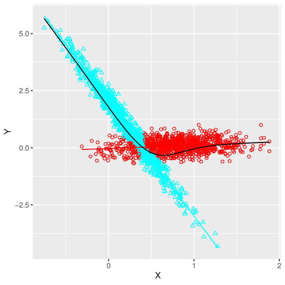
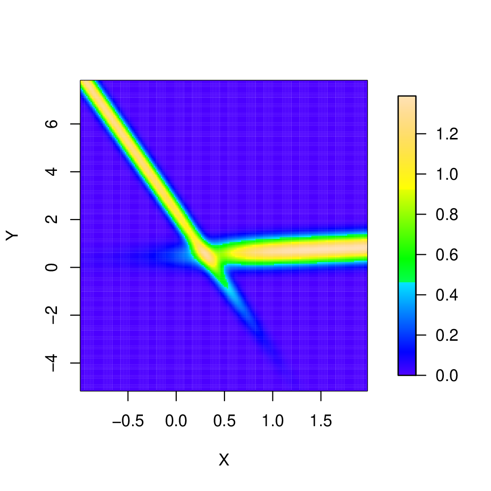
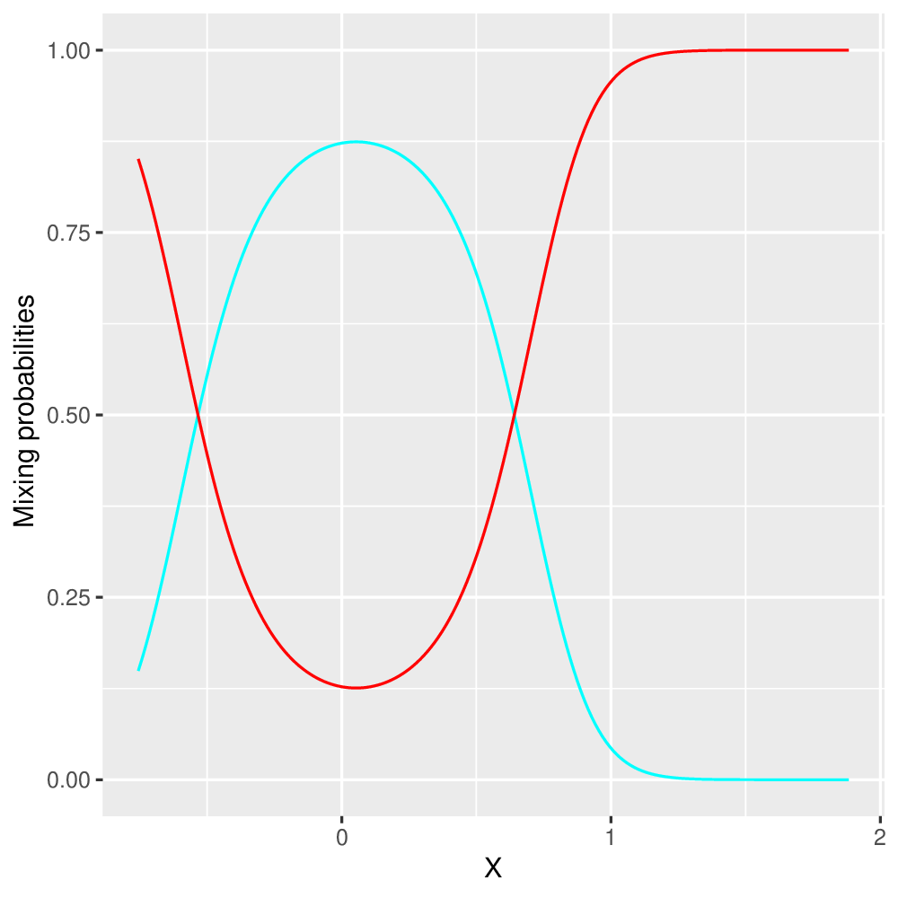
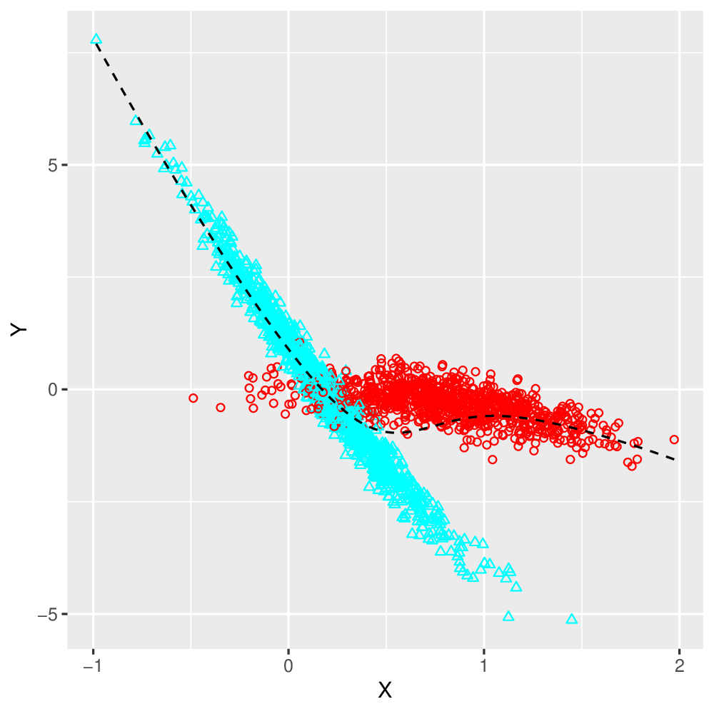
We wish to provide some simulated examples of GLoME regression models on $1$ -dimensional data sets, that is, with $L = D = 1$ . We construct simulated data sets following two scenarios: a well-specified (WS) case in which the true forward conditional density $s_{0}^{*}$ , which can be estimated via an affine Gaussian mean instance of GLoME, namely GLLiM model, based on inverse conditional PDF $s_{𝝍_{K, d}}$ using inverse regression strategy, belongs to the class of proposed models:

	$s_{0}^{*} (y \| x)$	$= \frac{ϕ (x; 0.2, 0.1)}{ϕ (x; 0.2, 0.1) + ϕ (x; 0.8, 0.15)} ϕ (y; - 5 x + 2, 0.09)$
		$+ \frac{ϕ (x; 0.8, 0.15)}{ϕ (x; 0.2, 0.1) + ϕ (x; 0.8, 0.15)} ϕ (y; 0.1 x, 0.09),$

and a misspecified (MS) case, whereupon such an assumption is not true:

	$s_{0}^{*} (y \| x)$	$= \frac{ϕ (x; 0.2, 0.1)}{ϕ (x; 0.2, 0.1) + ϕ (x; 0.8, 0.15)} ϕ (y; x^{2} - 6 x + 1, 0.09)$
		$+ \frac{ϕ (x; 0.8, 0.15)}{ϕ (x; 0.2, 0.1) + ϕ (x; 0.8, 0.15)} ϕ (y; - 0.4 x^{2}, 0.09) .$

Here we assume that the true number of mixture components $K_{0} = 2$ .

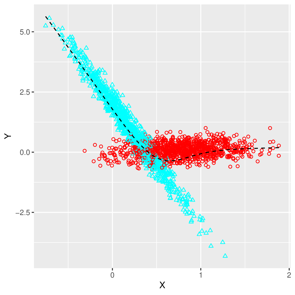
Figures 1.5(a) and 1.5(e) show some typical realizations of 2000 data points arising from the WS and MS scenarios. Note that by using GLLiM, the penalized maximum likelihood estimator of GLLiM, as introduced in Sections 1.2.3 and LABEL:chapter_ModelSelectionMoEs, performs well in the WS setting (Figures 1.5(b) to 1.5(d)). In the MS case, we expect our procedure, namely the GLLiM-EM algorithm introduced in LABEL:numericalExperiment, using slope heuristic, see Section 1.2.4 for more details, to automatically balance the model bias and its variance (Figures 1.5(f) to 1.5(h)), which leads to the choice of a complex model, with $4$ mixture components. This observation will be elaborated upon in the subsequent descriptions and experiments, see Sections 1.2.3, 1.2.4 and LABEL:numericalExperiment, respectively.

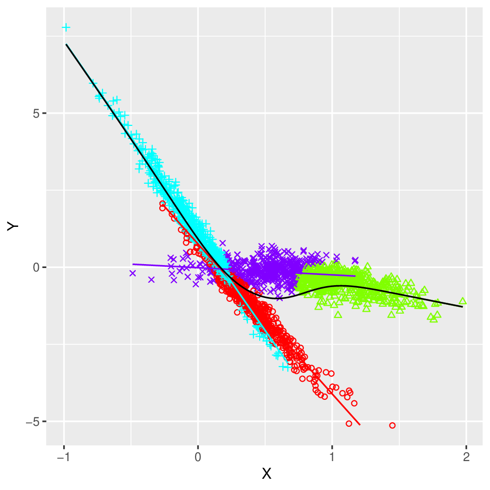
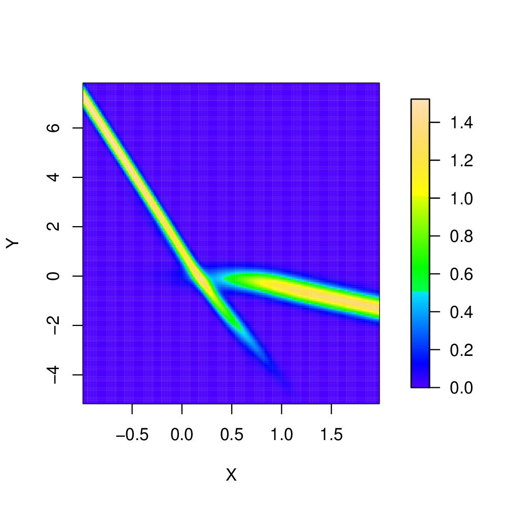
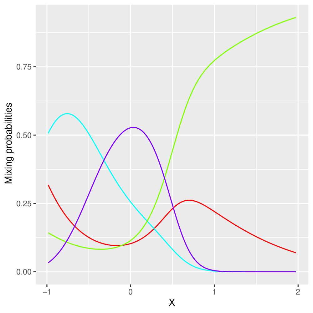
In the BLoME model, we wish to make use of block-diagonal structures by replacing $𝚺_{k}$ and $𝐕_{K}$ by $𝚺_{k} (𝐁_{k})$ and $𝐕_{K} (𝐁)$ , defined in (1.1.16), respectively (see, e.g., Devijver et al., 2017; Devijver and Gallopin, 2018; Nguyen et al., 2021b, ). This block-diagonal structures for covariance matrices are not only used for a trade-off between complexity and sparsity but also motivated by some real applications, where we want to perform prediction on data sets with heterogeneous observations and hidden graph-structured interactions between covariates; for instance, for gene expression data sets in which conditionally on the phenotypic response, genes interact with few other genes only, i.e., there are small modules of correlated genes (see Devijver et al., 2017; Devijver and Gallopin, 2018 for more details). To be more precise, for $k \in [K]$ , we decompose $𝚺_{k} (𝐁_{k})$ into $G_{k}$ blocks, $G_{k} \in ℕ^{⋆}$ , and we denote by $d^{[g]}_{k}$ the set of variables into the $g$ th group, for $g \in [G_{k}]$ , and by $c a r d (d^{[g]}_{k})$ the number of variables in the corresponding set. Then, we define $𝐁_{k} = (d^{[g]}_{k})_{g \in [G_{k}]}$ to be a block structure for the cluster $k$ , and $𝐁 = (𝐁_{k})_{k \in [K]}$ to be the covariate indexes into each group for each cluster. In this way, to construct the block-diagonal covariance matrices, up to a permutation, we make the following definition: $𝐕_{K} (𝐁) = (𝐕_{k} (𝐁_{k}))_{k \in [K]}$ , for every $k \in [K]$ ,

𝐕_{k} (𝐁_{k}) = {𝚺_{k} (𝐁_{k}) \in 𝒮_{D}^{+ +} | \begin{matrix} 𝚺_{k} (𝐁_{k}) = 𝐏_{k} (\begin{matrix} 𝚺_{k}^{[1]} & 𝟎 & \dots & 𝟎 \\ 𝟎 & 𝚺_{k}^{[2]} & \dots & 𝟎 \\ 𝟎 & 𝟎 & ⋱ & 𝟎 \\ 𝟎 & 𝟎 & \dots & 𝚺_{k}^{[G_{k}]} \end{matrix}) 𝐏^{- 1}_{k}, \\ 𝚺_{k}^{[g]} \in 𝒮^{+ +}_{c a r d (d^{[g]}_{k})}, \forall g \in [G_{k}] \end{matrix}},

(1.1.16)

where $𝐏_{k}$ corresponds to the permutation leading to a block-diagonal matrix in cluster $k$ . It is worth pointing out that outside the blocks, all coefficients of the matrix are zeros and we also authorize reordering of the blocks: e.g., ${(1, 3); (2, 4)}$ is identical to ${(2, 4); (1, 3)}$ , and the permutation inside blocks: e.g., the partition of $4$ variables into blocks ${(1, 3); (2, 4)}$ is the same as the partition ${(3, 1); (4, 2)}$ .

It is interesting to point out that GLLiM and BLLiM models in Deleforge et al., 2015c ; Devijver et al., (2017) are affine instances of GLoME and BLoME models, respectively, where linear combination of bounded functions (e.g., polynomials) are considered instead of affine mean functions for the Gaussian experts. The BLLiM framework aims to model a sample of high-dimensional regression data issued from a heterogeneous population with hidden graph-structured interaction between covariates. In particular, the BLLiM model is considered as a good candidate for performing model-based clustering and for predicting the response in situations affected by the “curse of dimensionality” phenomenon, where the number of parameters could be larger than the sample size. Indeed, to deal with high-dimensional regression problems, the BLLiM model is based on an inverse regression strategy, which inverts the role of the high-dimensional predictor and the multivariate response. Therefore, the number of parameters to estimate is drastically reduced. More precisely, BLLiM utilizes GLLiM, described in Deleforge et al., 2015a ; Deleforge et al., 2015c , in conjunction with a block-diagonal structure hypothesis on the residual covariance matrices to make a trade-off between complexity and sparsity.

This prediction model is fully parametric and highly interpretable. For instance, it might be useful for the analysis of transcriptomic data in molecular biology to classify observations or predict phenotypic states, as for example disease versus non disease or tumor versus normal (Golub et al., 1999; Nguyen and Rocke, 2002; Lê Cao et al., 2008). Indeed, if the predictor variables are gene expression data measured by microarrays or by the RNA-seq technologies and the response is a phenotypic variable, situations affected by the BLLiM not only provides clusters of individuals based on the relation between gene expression data and the phenotype, but also implies a gene regulatory network specific to each cluster of individuals (see Devijver et al., 2017 for more details).

1.1.2 SGaME and LinBoSGaBloME models

We will consider the statistical frameworks in which we model a sample of high-dimensional regression data issued from a heterogeneous population via a suitable MoE model with softmax gating functions. We emphasize that the dimension of the input $𝐗 \in 𝒳 \subset ℝ^{p}$ and/or the output $𝐘 \in 𝒴 \subset ℝ^{q}$ variable are/is typically much higher than the sample size $n$ . In this thesis, based on the original MoE models from Jacobs et al., (1991), we aim to establish a MoE model with softmax gating functions as generic as possible such that it can be used to handle with high-dimensional regression datasets and to study oracle inequalities. To do that, we first define $s_{𝝍_{K}} (𝐲 | 𝐱)$ to be a conditional PDF of MoE model as follows:

	$s_{𝝍_{K}} (𝐲 \| 𝐱)$	$= \sum_{k = 1}^{K} g_{𝐰, k} (𝐱) ϕ_{q} (𝐲; 𝝊_{k} (𝐱), 𝚺_{k} (𝐁_{k})), where,$		(1.1.17)
	$g_{𝐰, k} (𝐱)$	$= \frac{\exp (w_{k} (𝐱))}{\sum_{l = 1}^{K} \exp (w_{l} (𝐱))}, 𝐰 (𝐱) = (w_{k} (𝐱))_{k \in [K]} .$		(1.1.18)

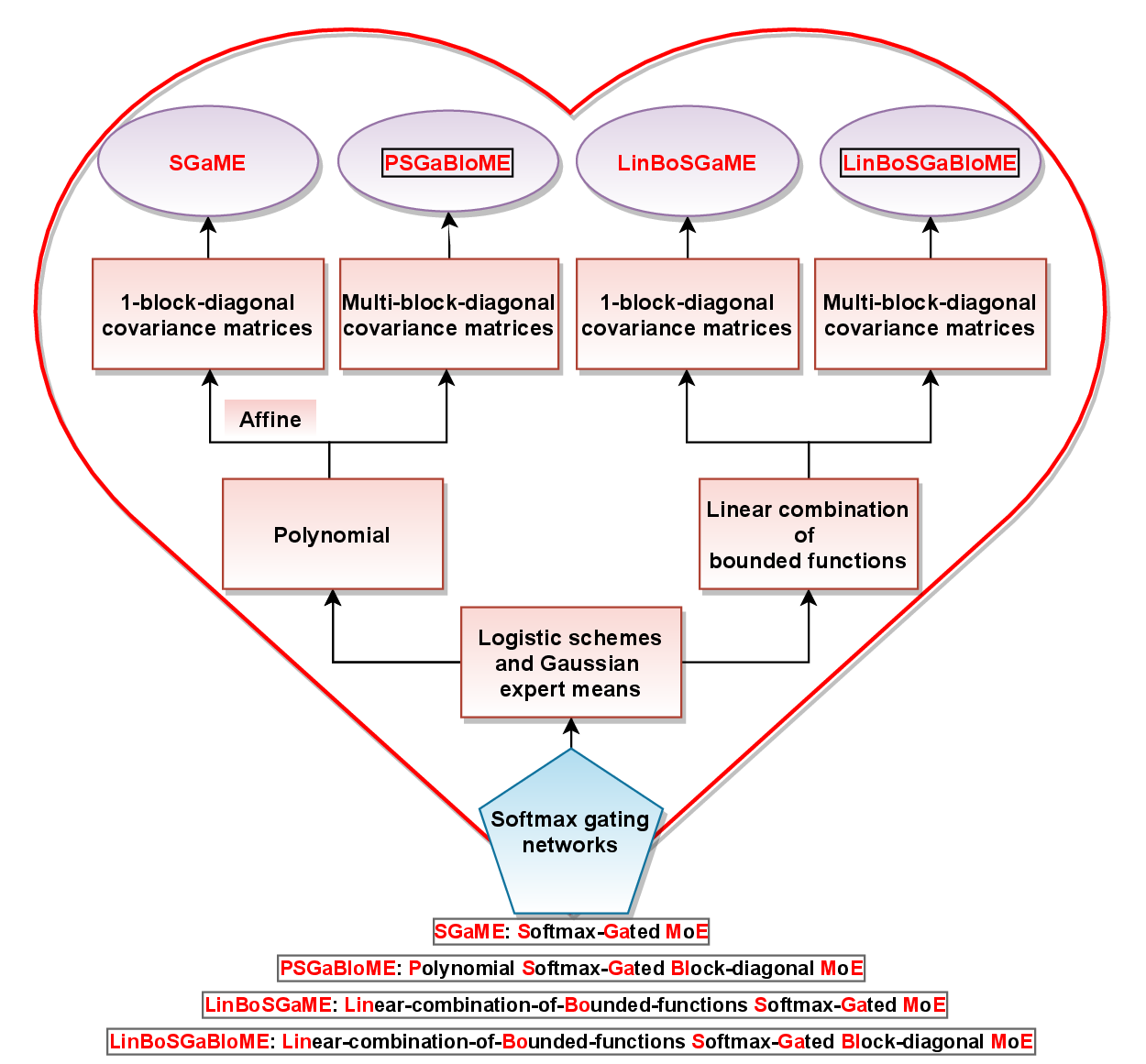
Here, $g_{𝐰, k} (\cdot)$ and $ϕ_{q} (\cdot; 𝝊_{k} (\cdot), 𝚺_{k} (𝐁_{k})), k \in [K]$ , are called softmax gating functions (or gating networks) and Gaussian experts, respectively. Note that for every $𝐱 \in 𝒳$ , $(g_{𝐰, k} (𝐱))_{k \in [K]} \in 𝚷_{K - 1}$ . Furthermore, we decompose the set of model parameters as follows: $𝝍_{K} = (𝐰, 𝝊, 𝚺) \in 𝐖_{K} \times 𝚼_{K} \times 𝐕_{K} (𝐁) = : 𝚿_{K}$ , $𝐰 = (w_{k})_{k \in [K]} \in 𝐖_{K}$ , $𝝊 = (𝝊_{k})_{k \in [K]} \in 𝚼_{K}$ , and $𝚺 (𝐁) = (𝚺_{k} (𝐁_{k}))_{k \in [K]} \in 𝚺_{k} (𝐁_{k})$ . It is worth noting that $𝐖_{K}$ and $𝚼_{K}$ are sets of $K$ -tuples of functions defined in logistic schemes (weights) and mean functions from $ℝ^{p}$ to $ℝ^{+}$ and $ℝ^{p}$ to $ℝ^{q}$ , respectively; and $𝚺_{k} (𝐁_{k})$ is a set containing $K$ -tuples of $𝒮_{q}^{+ +}$ with the block-diagonal structures defined in (1.1.16), where $𝒮_{q}^{+ +}$ denotes the collection of symmetric positive definite matrices on $ℝ^{q}$ . Since we need to bound the model complexity using the dimension of model, we have to restrict our attention to LinBoSGaBloME models, where $𝐖_{K}$ and $𝚼_{K}$ are defined as the linear combination of a finite set of bounded functions whose coefficients belong to a compact set. When the dimension of both inputs and outputs are not too large, we do not need to select relevant variables. Then, we can work on the previous LinBoSGaBloME models with general structures for means, weights and multi-block-diagonal covariance matrices. In some situation, we do not need to take into account the trade-off between complexity and sparsity for covariance matrices, in LinBoSGaBloME models, we can consider $1$ -block-diagonal covariance matrices, which is well studied in Montuelle et al., (2014) and will be referred to be as linear-combination-of-bounded-functions softmax-gated mixture of experts (LinBoSGaME) regression models. However, to deal with high-dimensional data and to simplify the interpretation of sparsity, in LinBoSGaBloME model, we propose to utilize polynomials for the weights of the softmax gating functions and the Gaussian expert means, which will be referred to as polynomial softmax-gated block-diagonal mixture of experts (PSGaBloME) regression models. In particular, we simply refer to affine instances of LinBoSGaBloME models as softmax-gated mixture of experts (SGaME) regression models. Compared to the general PSGaBloME model, SGaME model is defined based on 1-block-diagonal covariance matrices. This means that we do not impose the potential hidden graph-structured interactions between covariate variables. Furthermore, instead of using a linear combination of a finite set of bounded functions whose coefficients belong to a compact set, SGaME models utilize the linear functions for both the weights of softmax gating networks and the means of Gaussian experts. The readers are referred to Figure 1.6 for comprehensive classification and nomenclature of standard MoE regression models with softmax gating networks.

1.2 Model selection in mixtures of experts regression models

It is worth pointing out that several hyperparameters must be estimated to construct BLoME and PSGaBloME regression models, including the number of mixtures components (or clusters), the block structure of large covariance matrices specific of each cluster (the size and the number of blocks), the degree of polynomials appearing in gating networks and Gaussian mean experts, the relevant variables and rank sparse models in PSGaBloME. Data driven choices of hyperparameters of learning algorithms belong to the model selection class of problems, which has attracted much attention in statistics and machine learning over the last 50 years (Akaike, 1974; Mallows, 1973; Anderson and Burnham, 2002; Massart, 2007). This is a particular instance of the estimator (or model) selection problem: given a family of estimators, how do we choose, using data, one among them whose risk is as small as possible? Note that penalization is one of the main strategies proposed for model selection. It suggests to choose the estimator minimizing the sum of its empirical risk and some penalty terms corresponding to how well the model fits the data, while avoiding overfitting.

In this thesis, we are interested in controlling and accounting for model complexity when selecting the best number of mixture components of a model. In general, model selection is often performed using the Akaike information criterion (AIC; Akaike, 1974) or the Bayesian information criterion (BIC; Schwarz et al., 1978). An important limitation of these criteria, however, is that they are only valid asymptotically. This implies that there are no finite sample guarantees when using AIC or BIC, for choosing between different levels of complexity. Their use in small sample settings is thus ad hoc. To overcome such difficulties, Birgé and Massart, (2007) proposed a novel approach, called slope heuristics, supported by a non-asymptotic oracle inequality. This method leads to an optimal data-driven choice of multiplicative constants for penalties. Recent reviews and practical issues regarding the slope heuristic can be found in Baudry et al., (2012), Arlot, (2019), and the references given therein.

It should be stressed that a general model selection result, originally established by Massart, (2007, Theorem 7.11), guarantees a penalized criterion leads to a good model selection and the penalty being only known up to multiplicative constants and proportional to the dimensions of models. In particular, such multiplicative constants can be calibrated by the slope heuristic approach in a finite sample setting. Then, in the spirit of the concentration inequality-based methods developed in Massart, (2007), Massart and Meynet, (2011), and Cohen and Le Pennec, (2011), a number of finite-sample oracle results have been established for the least absolute shrinkage and selection operator (LASSO) (Tibshirani, 1996) and general penalized maximum likelihood estimators (PMLE). These results include the works for high dimensional Gaussian graphical models (Devijver and Gallopin, 2018), Gaussian mixture model selection (Maugis and Michel, 2011b, ; Maugis and Michel, 2011a, ), finite mixture regression models (Meynet, 2013; Devijver, 2015a, ; Devijver, 2015b, ; Devijver, 2017b, ; Devijver, 2017a, ), SGaME models without considering high-dimensional setting (Montuelle et al., 2014).

No attempt has been made in the literature to develop a finite-sample oracle inequality for MoE regression models framework for high-dimensional data. In this thesis, to the best of our knowledge, we are the first to provide finite-sample oracle inequalities for several high-dimensional MoE regression models, including the GLoME model (Nguyen et al., 2021c, LABEL:section_nguyen2021nonGLoME), BLoME model (Nguyen et al., 2021b, LABEL:section_nguyen2021nonBLoME), SGaME model using LASSO (Nguyen et al., 2020c, LABEL:section_nguyen2020l1oracle), and PSGaBloME model (LABEL:section_nguyen2021joint). In particular, our proof strategy makes use of recent novel approaches comprising a model selection theorem for the maximum likelihood estimator (MLE) among a random subcollection (Devijver, 2015b, ), a non-asymptotic model selection result for detecting a good block-diagonal structure in high-dimensional graphical models (Devijver and Gallopin, 2018) and a reparameterization trick to bound the metric entropy of the Gaussian gating parameter space in GLoME models (Nguyen et al., 2021c, ), see also LABEL:section_nguyen2021nonGLoME for more details. Note that for the Gaussian gating parameters, the technique for handling the logistic weights in the SGaME models of Montuelle et al., (2014) is not directly applicable to the GLoME or BLoME framework, due to the quadratic form of the canonical link. Therefore, we propose a reparameterization trick¹¹1Note that we only use this nomenclature to perform a change of variables of the Gaussian gating parameters space of GLoME models via the logistic weights of SGaME models. This reparameterization trick does not stand for the well-known one of Variational Autoencoders (VAEs) in the deep learning literature (see Kingma and Welling, 2013, for more details). to bound the metric entropy of the Gaussian gating parameters space; see LABEL:eq_reparameterizationTrick and LABEL:sec_proof_lem_Bracketing_Entropy_Gates for more details. Furthermore, in Nguyen et al., 2021c (, LABEL:weakOracleInequality), see also LABEL:section_nguyen2021nonGLoME, we extend one of corollaries (in which the authors used linear combination of bounded functions for the functions in softmax gating networks) from Montuelle et al., (2014, Theorem 1) to the quadratic form of the canonical link from gating networks, see more details in LABEL:eq_reparameterizationTrick and LABEL:lem_Bracketing_Entropy_Gates.

Among of the main contributions of this thesis are the important theoretical results: finite-sample oracle inequalities that provide non-asymptotic bounds on the risks, and lower bounds on the penalty functions that ensure non-asymptotic theoretical controls on the estimators under the Jensen–Kullback–Leibler loss. These oracle inequalities also provide some theoretical justifications of the penalty shapes when using the slope heuristic for GLLiM, GLoME, BLLiM, BLoME, SGaME, and PSGaBloME models. We emphasize that although the finite-sample oracle inequalities compare performances of our estimators with the best model in the collection, they also allow us to well approximate a rich class of conditional densities if we take enough degree of polynomials of Gaussian expert means (belongs to $𝒟_{𝚼}$ ) and/or enough clusters (among the set $𝒦$ ) in the context of mixture of Gaussian experts (Jiang and Tanner, 1999a, ; Mendes and Jiang, 2012; Nguyen et al., 2016; Ho et al., 2019; Nguyen et al., 2021a, ). This leads to the upper bounds on the risks being small, for $𝒟_{𝚼}$ and $𝒦$ well-chosen.

Especially, aside from important theoretical issues regarding the tightness of the bounds, the way to integrate a priori information and the minimax analysis of our proposed PMLE, we hope that our finite-sample oracle inequalities and corresponding interesting numerical experiments help to partially answer the two following important questions raised in the area of MoE regression models: (1) What number of mixture components $K$ should be chosen, given the sample size $n$ , and (2) Whether it is better to use a few complex experts or combine many simple experts, given the total number of parameters. Note that, such problems are considered in the work of Mendes and Jiang, (2012, Proposition 1), where the authors provided some qualitative insights and only suggested a practical method for choosing $K$ and $d$ involving a complexity penalty or cross-validation. Furthermore, their model is only for a non-regularized maximum-likelihood estimation, and thus is not suitable in the high-dimensional setting.

In this thesis, we will consider the parameter selection problem as a model selection problem, by constructing a collection of models, with more or less clusters, complex or simple experts controlling via the orders of polynomial of weights and Gaussian experts, high or low rank sparse models, and more or less active coefficients. Then, it will remain to choose a model among this collection. In general, let us denote by $𝒮 = (S_{𝐦})_{𝐦 \in ℳ}$ the collection of models that we consider, indexed by $ℳ$ . It is worth pointing out that, in contrary to what one might think, having a collection of models that is too large can be detrimental, for example by selecting inconsistent estimators (Bahadur, 1958) or suboptimal estimators (Birgé and Massart, 1993). This is the called model selection paradigm.

Before discussing the finite-sample oracle inequalities for model selection via penalization in MoE regression models, we review some standard facts regarding estimation by contrast minimization.

1.2.1 Minimum contrast estimation

The minimum contrast estimation method is based on the existence of a contrast function, denoted by $γ$ , fulfilling the fundamental property that the unknown conditional PDF satisfies

s_{0} = a r g m i n_{t \in 𝒮} 𝔼_{𝐗, 𝐘} [γ (t, 𝐗, 𝐘)] .

In this way we obtain what will be referred to as the associated loss function, denoted $l$ , that is defined via

l (s_{0}, t) = 𝔼_{𝐗, 𝐘} [γ (t, 𝐗, 𝐘)] - 𝔼_{𝐗, 𝐘} [γ (s_{0}, 𝐗, 𝐘)], \forall t \in 𝒮 .

Let us define some empirical contrast $γ_{n}$ (based on the observation $(𝐗_{[n]}, 𝐘_{[n]}) : = (𝐗_{i}, 𝐘_{i})_{i \in [n]}$ ) such that

\forall t \in 𝒮, γ_{n} (t) = \frac{1}{n} \sum_{i = 1}^{n} γ (t, 𝐗_{i}, 𝐘_{i}) .

For the model $𝐦$ , a minimum contrast estimator $\hat{s}_{𝐦}$ of $s_{0}$ is a minimizer of the empirical contrast $γ_{n}$ over $S_{𝐦}$ , i.e., $\hat{s}_{𝐦} = a r g m i n_{t \in S_{𝐦}} γ_{n} (t)$ . The idea is that, under reasonable conditions, $γ_{n} (t)$ converges to $𝔼_{𝐗, 𝐘} [γ (t, 𝐗, 𝐘)]$ , and that there is some hope to get a sensible estimator of $s_{0}$ , at least if $s_{0}$ belongs (or is close enough) to model $S_{𝐦}$ . To measure the quality of such an estimator, we make use of the following risk $ℛ (\hat{s}_{𝐦}) = 𝔼_{𝐗_{[n]}, 𝐘_{[n]}} [l (s_{0}, \hat{s}_{𝐦})]$ .

For example, in the density estimation framework, the popular maximum likelihood estimator is a minimum contrast estimator. Indeed, we assume that the sample $(𝐗_{i}, 𝐘_{i})_{i \in [n]}$ has the density $s_{0}$ w.r.t. a measure $μ$ and consider another density $t$ w.r.t. the same measure. Then, the negative log-likelihood $- \ln [t (𝐲 | 𝐱)]$ is the maximum likelihood contrast, and the corresponding loss function is the Kullback–Leibler divergence defined by $K L (s_{0}, t) = \int s_{0} \ln (\frac{s_{0}}{t}) d μ$ . For a fuller treatment regarding other examples of contrast for regression, classification and Gaussian white noise, we refer the reader to Massart, (2007).

1.2.2 The model choice paradigm

The purpose is to select the “best” estimator among the collection $(\hat{s}_{𝐦})_{𝐦 \in ℳ}$ . Let $S_{\hat{𝐦}}$ be the model selected by a given model selection procedure. We will denote by $\hat{s}_{\hat{𝐦}}$ the selected estimator and emphasize that both $\hat{s}_{𝐦}$ (for any $𝐦$ ) and $\hat{𝐦}$ are built from the same sample $(𝐗_{[n]}, 𝐘_{[n]})$ . This procedure has been well studied from both an asymptotic and a non-asymptotic point of view.

Ideally, for a given $n$ and a given dataset, one would like to consider $𝐦^{*}$ minimizing the risk $𝔼_{𝐗_{[n]}, 𝐘_{[n]}} [l (s_{0}, \hat{s}_{𝐦})]$ , with respect to $𝐦 \in ℳ$ . In other words,

𝐦^{*} \in \arg \min_{𝐦 \in ℳ} l (s_{0}, \hat{s}_{𝐦}) .

(1.2.1)

The minimum contrast estimator $\hat{s}_{𝐦^{*}}$ on the corresponding model $S_{𝐦^{*}}$ is called an oracle. This terminology has previously been introduced by Donoho and Johnstone, (1994). Unfortunately, since the loss $l (s_{0}, \hat{s}_{𝐦})$ depends on the unknown sample distribution $s_{0}$ , thus so does $𝐦^{*}$ and the oracle $\hat{s}_{𝐦^{*}}$ should not be an estimator of $s_{0}$ . However, this oracle can serve as a benchmark for building any data driven selection procedure among the collection of estimators $(\hat{s}_{𝐦})_{m \in ℳ} .$ It is now natural to consider data-driven criteria to select an estimator which tends to mimic an oracle. In other words, we would like the risk of the selected estimator $\hat{s}_{\hat{𝐦}}$ , i.e., $𝔼_{𝐗_{[n]}, 𝐘_{[n]}} [l (s_{0}, \hat{s}_{\hat{𝐦}})]$ , to be as close as possible to the risk of an oracle, i.e., $𝔼_{𝐗_{[n]}, 𝐘_{[n]}} [l (s_{0}, \hat{s}_{𝐦^{*}})]$ .

It is worth pointing out that the non-asymptotic approach (see, e.g., Massart, 2007; Wainwright, 2019 for the complete bibliography) differs from the usual asymptotic point of view in the sense that the number as well as the dimensions of the models in $ℳ$ may depend on $n$ . We wish to construct a model selection procedure such that the selected model $S_{\hat{𝐦}}$ is optimal. For instance, it fulfills the following oracle inequality

l (s_{0}, \hat{s}_{\hat{𝐦}}) \leq C_{1} l (s_{0}, \hat{s}_{𝐦^{*}}) + \frac{C_{2}}{n}

(1.2.2)

with $C_{1}$ as close to $1$ as possible and $C_{2} / n$ a remainder term. The oracle inequality is said to be exact if $C_{1} = 1$ . We expect that this inequality holds either in expected value or with high probability. In particular, when such results are too difficult to be achieved, it suffices to obtain a weaker form:

𝔼_{𝐗_{[n]}, 𝐘_{[n]}} [l (s_{0}, \hat{s}_{\hat{𝐦}})] \leq C_{1} i n f_{𝐦 \in ℳ} 𝔼_{𝐗_{[n]}, 𝐘_{[n]}} [l (s_{0}, \hat{s}_{𝐦^{*}})] + \frac{C_{2}}{n} .

(1.2.3)

1.2.3 Model selection via penalization

Now, let us describe how to select a model via minimizing a penalized criterion, to reach a bias/variance compromise. Indeed, we can decompose the loss into a bias and a variance parts as follows:

	$l (s_{0}, \hat{s}_{𝐦})$	$= 𝔼_{𝐗, 𝐘} [γ (\hat{s}_{𝐦}, 𝐗, 𝐘)] - 𝔼_{𝐗, 𝐘} [γ (s_{0}, 𝐗, 𝐘)]$
		$= 𝔼_{𝐗, 𝐘} [γ (s_{𝐦}, 𝐗, 𝐘)] - 𝔼_{𝐗, 𝐘} [γ (s_{0}, 𝐗, 𝐘)] - 𝔼_{𝐗, 𝐘} [γ (s_{𝐦}, 𝐗, 𝐘)] + 𝔼_{𝐗, 𝐘} [γ (\hat{s}_{𝐦}, 𝐗, 𝐘)]$
		$= \underset{⏟}{l (s_{0}, s_{𝐦})}_{bias} + \underset{⏟}{𝔼_{𝐗, 𝐘} [γ (\hat{s}_{𝐦}, 𝐗, 𝐘) - γ (s_{𝐦}, 𝐗, 𝐘)]}_{variance},$

where $s_{𝐦} = a r g m i n_{t \in S_{𝐦}} 𝔼_{𝐗, 𝐘} [γ (t, 𝐗, 𝐘)]$ is one of the best approximations of $s_{0}$ in $S_{𝐦}$ . It is worth pointing out that in order to minimize the bias, we need a complex model, which fits very closely to the data; and to minimize the variance, we should not consider too complex models, in order to avoid overfitting of the data.

The main methods to account for such model selection procedures are cross-validation and hold-out (see, e.g., Arlot and Celisse, 2010; Maillard, 2020 for the complete bibliography), or penalized criteria. It is emphasized that the main difficulty in carrying out the cross-validation and hold-out is time complexity, particularly in high-dimensional setting. Therefore, the choice of penalization criteria seems to the best adapted to our high-dimensional MoE regression models.

Let us describe the method in more details. The model selection via penalization procedure consists in considering some proper penalty function $pen: ℳ \to ℝ_{+}$ and taking $\hat{𝐦}$ that minimizes the penalized criterion, defined as $γ_{n} (\hat{s}_{𝐦}) + pen (𝐦)$ over $ℳ$ . This means that we select

\hat{𝐦} = a r g m i n_{𝐦 \in ℳ} {γ_{n} (\hat{s}_{𝐦}) + pen (𝐦)} .

(1.2.4)

In other words, in the context of the maximum likelihood estimator for the regression case, for a given choice of $p e n (𝐦)$ , the selected model $S_{\hat{𝐦}}$ is chosen as the one whose index is an $η^{'}$ -almost minimizer of the sum of the negative log-likelihood (NLL) and this penalty:

\sum_{i = 1}^{n} - \ln (\hat{s}_{\hat{𝐦}} (𝐱_{i} | 𝐲_{i})) + p e n (\hat{𝐦}) \leq i n f_{𝐦 \in ℳ} (\sum_{i = 1}^{n} - \ln (\hat{s}_{𝐦} (𝐱_{i} | 𝐲_{i})) + p e n (𝐦)) + η^{'} .

(1.2.5)

Here, $\hat{s}_{𝐦}$ is defined as the $η$ -minimizer of the NLL:

\sum_{i = 1}^{n} - \ln (s_{\hat{s}_{𝐦}} (𝐱_{i} | 𝐲_{i})) \leq i n f_{s_{𝐦} \in S_{𝐦}} \sum_{i = 1}^{n} - \ln (s_{𝐦} (𝐱_{i} | 𝐲_{i})) + η,

(1.2.6)

where the error term $η$ is necessary when the infimum may not be unique or even not be reached. Note that $\hat{s}_{\hat{𝐦}}$ is then called the $η^{'}$ -penalized likelihood estimator and depends on both the error terms $η$ and $η^{'}$ . From hereon in, the terms “best data-driven model or estimate” and “selected model or estimator” are both used to indicate that it satisfies (1.2.5).

We emphasize that choosing the penalty is tricky but obviously necessary. The construction of such functions in the context of maximum likelihood estimator goes back to the work of Akaike and Schwarz, see respectively Akaike, (1974) and Schwarz et al., (1978). They proposed the now classic AIC and BIC criteria, the two most widely known and pervasively used tools in statistical model selection, where the penalty is respectively establish as follows:

	$p e n_{AIC} (𝐦)$	$= D_{𝐦},$
	$p e n_{BIC} (𝐦)$	$= \frac{\ln (n) D_{𝐦}}{2},$

where $D_{𝐦}$ is the dimension of the model $𝐦$ , and $n$ is the size of the sample considered. These well-known penalized criteria have been widely studied (see, e.g., Anderson and Burnham, 2002) and based on asymptotic approximations. Therefore, such criteria may be wrong in a non-asymptotic context. More precisely, AIC and BIC are based on Wilks’ theorem and a Bayesian approach, see, e.g., Cavanaugh and Neath, (2019) and Neath and Cavanaugh, (2012), respectively, for recent reviews on the conceptual and theoretical foundations. At the same time, Mallows, (1973), and later Craven and Wahba, (1978) proposed other famous penalized criteria: Mallows’s $C_{p}$ and generalized cross-validation (GCV), respectively, in the context of linear regression. Mathematically, Mallows obtained

p e n_{Mallows} (𝐦)

= \frac{2 D_{𝐦} σ^{2}}{n},

where $σ^{2}$ is noise level of the true regression model which is unknown (if it does exist) and $σ^{2}$ is thus difficult to estimate. Similarly, the solution proposed by the GCV method is based on cross-validation to choose the unknown tunning parameter (which best value is actually $σ^{2}$ ). Thus, again, we have to estimate an unknown parameter.

1.2.4 Slope heuristics

Motivated by some recent works on concentration inequalities, Birgé and Massart, (2001) introduced the slope heuristic, which is a non-asymptotic methodology to select a model from a collection of models. This slope heuristics allows us to choose an optimal penalties from data which are known up to a multiplicative constant $κ$ . Let us describe the ideas of this heuristic. In this framework, the penalty shape is then adapted as $p e n_{shape} (\cdot)$ and an unknown constant $κ_{opt}$ exists such that

p e n_{opt} : 𝐦 \in ℳ \mapsto κ_{opt} p e n_{shape} (𝐦)

is an optimal penalty. In order to select the oracle model via using (1.2.1) and (1.2.4), we are looking for a penalty close to the following penalty function:

ℳ ∋ 𝐦 \mapsto pen (𝐦) = l (s_{0}, \hat{s}_{𝐦}) - γ_{n} (\hat{s}_{𝐦}) .

However, since $s_{0}$ is unknown in practice, we will try to approach this quantity by decomposing it into:

$l (s_{0}, \hat{s}_{𝐦}) - γ_{n} (\hat{s}_{𝐦})$	$= 𝔼_{𝐗, 𝐘} [γ (\hat{s}_{𝐦}, 𝐗, 𝐘)] - 𝔼_{𝐗, 𝐘} [γ (s_{0}, 𝐗, 𝐘)] - γ_{n} (\hat{s}_{𝐦})$
	$= \underset{⏟}{𝔼_{𝐗, 𝐘} [γ (\hat{s}_{𝐦}, 𝐗, 𝐘)] - 𝔼_{𝐗, 𝐘} [γ (s_{𝐦}, 𝐗, 𝐘)]}_{ν_{𝐦}} + \underset{⏟}{[γ_{n} (s_{𝐦}) - γ_{n} (\hat{s}_{𝐦})]}_{\hat{ν}_{𝐦}}$
	$+ \underset{⏟}{𝔼_{𝐗, 𝐘} [γ (s_{𝐦}, 𝐗, 𝐘)] - 𝔼_{𝐗, 𝐘} [γ (s_{0}, 𝐗, 𝐘)]}_{(1)} - \underset{⏟}{[γ_{n} (s_{𝐦}) - γ_{n} (s_{0})]}_{(2)} - γ_{n} (s_{0}) .$	(1.2.7)

Here, $ν_{𝐦}$ is an “estimation error” term, $\hat{ν}_{𝐦}$ is an empirical “estimation error” term. We will denote by $Δ_{n} (s_{𝐦}) = (1) - (2)$ , which corresponds to the difference between the “bias” term and its empirical version. Note that $γ_{n} (s_{0})$ does not depend on $𝐦$ , the main idea is to estimate the following ideal penalty, defined as $p e n^{*} (𝐦) = ν_{𝐦} + \hat{ν}_{𝐦} + Δ_{n} (s_{𝐦})$ , from the data in order to build an optimal penalty function. Then, (1.2.4) implies that

l (s_{0}, \hat{s}_{𝐦}) - γ_{n} (\hat{s}_{𝐦}) = p e n^{*} (𝐦) - γ_{n} (s_{0}), \forall 𝐦 \in ℳ .

(1.2.8)

Next, we wish to prove the following oracle inequality

l (s_{0}, \hat{s}_{\hat{𝐦}}) + [p e n (\hat{𝐦}) - p e n^{*} (\hat{𝐦})] \leq i n f_{𝐦 \in ℳ} {l (s_{0}, \hat{s}_{𝐦}) + [p e n (𝐦) - p e n^{*} (𝐦)]} .

(1.2.9)

Indeed, by definition of the ideal penalty by (1.2.8), and the fact that $\hat{m} \in ℳ$ , it holds that for all $𝐦 \in ℳ$ ,

	$l (s_{0}, \hat{s}_{\hat{𝐦}}) + [p e n (\hat{𝐦}) - p e n^{*} (\hat{𝐦})]$	$= γ_{n} (\hat{s}_{\hat{𝐦}}) + p e n (\hat{𝐦}) - γ_{n} (s_{0})$
		$\leq γ_{n} (\hat{s}_{𝐦}) + p e n (𝐦) - γ_{n} (s_{0}) (using (1.2.4))$
		$= l (s_{0}, \hat{s}_{𝐦}) + [p e n (𝐦) - p e n^{*} (𝐦)] (using (1.2.8)) .$

The important point to note here is the form of (1.2.9) motivates us to look for a penalty close to the ideal penalty to obtain an oracle inequality. According to the expression of the ideal penalty $p e n^{*} (𝐦) = ν_{𝐦} + \hat{ν}_{𝐦} + Δ_{n} (s_{𝐦})$ , both $ν_{𝐦}$ and $Δ_{n} (s_{𝐦})$ depend on the unknown conditional PDF $s_{0}$ . Therefore, it is natural to try to relate the penalty function to the empirical estimation error term $\hat{ν}_{𝐦}$ .

To accomplish this task, from a theoretical point of view, Birgé & Massart, in Birgé and Massart, (2001, 2007) proposed and proved for the first time the slope heuristics method in the context of Gaussian homoscedastic least squares regression with fixed design. They prove that there exists a minimal penalty, $p e n_{min} (𝐦) = \hat{ν}_{𝐦}$ , namely such that the dimension and the risk of models selected with lighter penalties become very large, whereas higher penalties should select models with “reasonable” complexity. Furthermore, they show that considering a penalty equal to twice this minimal penalty allows to select a model close to the oracle model in terms of risk.

More precisely, given the chosen penalty as $p e n (𝐦) = κ \hat{ν}_{𝐦}$ , the penalized criterion can be written as

crit (𝐦) = (1 - κ) γ_{n} (\hat{s}_{𝐦}) + κ γ_{n} (s_{𝐦}) .

Therefore, three cases occur:

•

if $κ = 1$ then $crit (𝐦) = γ_{n} (s_{𝐦})$ , which concentrates around its expectation $𝔼_{𝐗, 𝐘} [γ (s_{𝐦}, 𝐗, 𝐘)] = \underset{⏟}{l (s_{0}, s_{𝐦})}_{bias} + 𝔼_{𝐗, 𝐘} [γ (s_{0}, 𝐗, 𝐘)]$ for large $n$ : this procedure selects a model minimizing the bias and does not take into account the variance, which leads to such criterion has “a significant probability”²²2Note that when $κ = 1$ , the probability to select a too complex model is in general positive but strictly below $1$ . Actually, this is general with slope heuristics / minimal penalty algorithms: with a data-driven criterion (hence a bit random), when the penalty is exactly at the minimal level, the selected model complexity is highly random (we are just at the critical state of the phase transition) Arlot, (2019). of selecting a too complex model;
•

if $κ < 1$ then when the complexity goes up, the criterion always goes down because of the two terms in $crit (𝐦)$ being dropping: the selected models is always one of the most complex ones;
•

if $κ > 1$ then the criterion rises with the complexity of the most complex models due to the fact that of ruling out the corresponding bias terms (these models almost have the same bias): the dimension of the selected models will be more reasonable.

The first point of the slope heuristics is $\hat{ν}_{𝐦} \approx ν_{𝐦}$ since $\hat{ν}_{𝐦}$ is the empirical counterpart of $ν_{𝐦}$ . In particular, it is expected that we can control the fluctuation of $Δ_{n} (s_{𝐦})$ around its zero expectations through concentration results. Therefore, we can approximate the ideal penalty as twice the minimal penalty due to the fact that

p e n^{*} (𝐦) = ν_{𝐦} + \hat{ν}_{𝐦} + Δ_{n} (s_{𝐦}) \approx 2 \hat{ν}_{𝐦} .

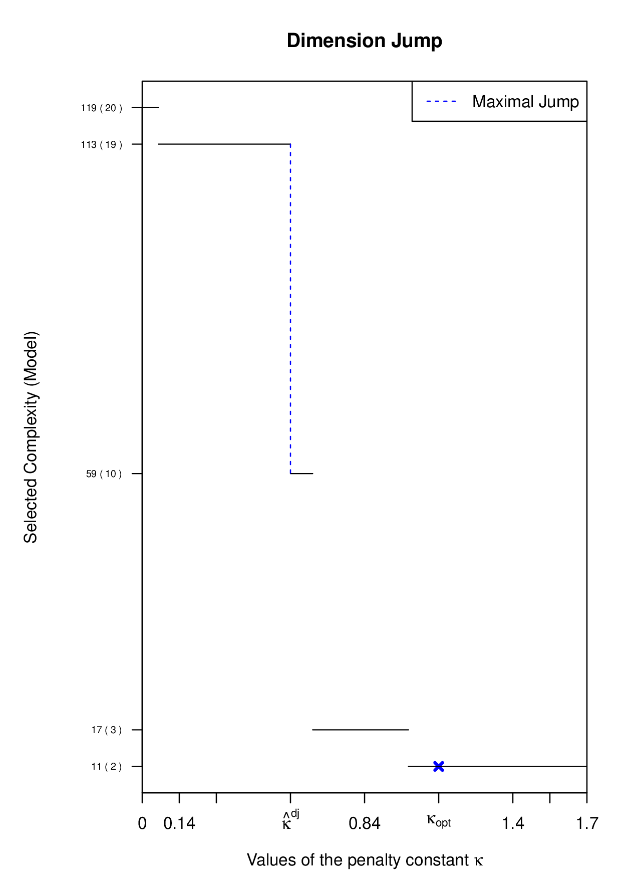
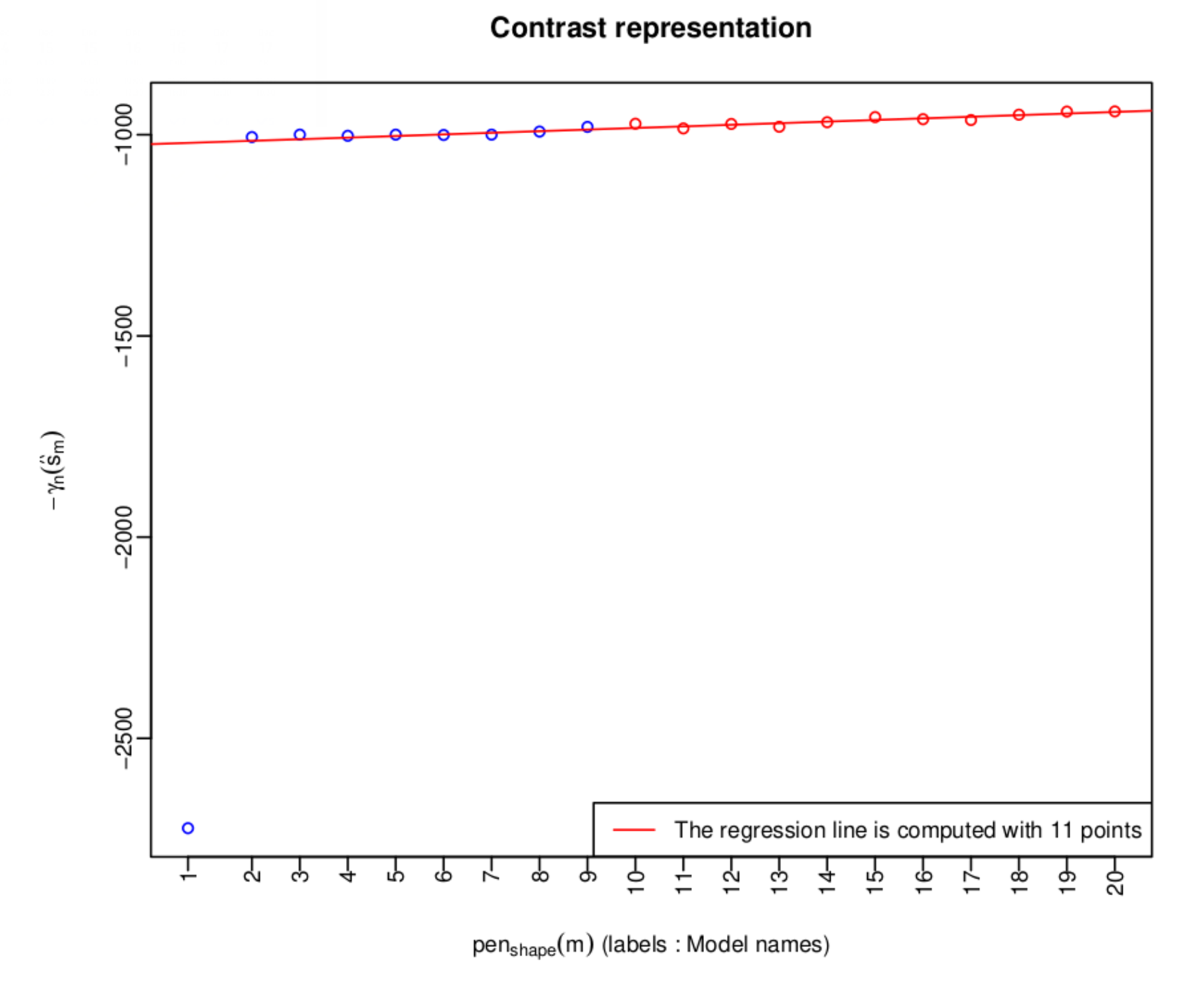
Thus, in practice, the main remaining issue is to determine the minimal penalty $\hat{ν}_{𝐦}$ . To this end, on the data set $(𝐗_{[n]}, 𝐘_{[n]})$ ; either we look for the greatest jump of complexity of the selected model as a function of the multiplicative constant $κ$ in the penalty or we look at the asymptotic slope of a linear regression between the penalty shape $p e n_{shape} (\cdot)$ and the contrast value $γ_{n} (s_{𝐦})$ for the most complex models, which will be referred to as dimension jump or data-driven slope estimation, respectively. In this way, we obtain the minimal penalty, and we multiply it by two to obtain the optimal penalty. For a deeper discussion of the principle of slope heuristics, we refer the reader to Baudry et al., (2012); Arlot, (2019) and the references given therein. Figures 1.7(a) and 1.7(b) illustrate these ideas.

We emphasize that from a practical point of view, we use the so-called CAPUSHE (CAlibrating Penalty Using Slope HEuristics) package in R (Arlot et al., 2016; Baudry et al., 2012) to implement the dimension jump and the data-driven slope estimation approaches. In practice, using slope heuristic is effective when an optimal penalty $p e n_{opt} (\cdot) = κ_{opt} p e n_{shape} (\cdot)$ is known up to a multiplicative factor. It is worth pointing out that the keystone of the slope heuristics is that $\frac{κ_{opt}}{2} p e n_{shape} (𝐦)$ is a good estimate of $\hat{s}_{𝐦}$ and provides a minimal penalty. Generally speaking, the $p e n_{shape} (\cdot)$ can be chosen as the complexity measure, when its definition is not obvious a priori. This complexity measure is typically the model dimension $D_{𝐦}$ or the number of free parameters needed to be estimated.

From a theoretical point of view, in this thesis, we contribute several non-asymptotic oracle inequalities, Theorems 1.2.3 and 1.2.4, which provide non-asymptotic bounds on the risks, and lower bounds on the penalty functions that ensure non-asymptotic theoretical controls on the estimators under the Jensen–Kullback–Leibler loss. These oracle inequalities also provide some theoretical justifications of the penalty shapes when using the slope heuristic for the corresponding MoE regression models. More precisely, penalized likelihood criteria are proposed in LABEL:chapter_ModelSelectionMoEs and LABEL:chapter_JointRankVariableMoEs to select best data-driven MoE regression models among a specific model collection. These criteria depend on unknown constants which can be calibrated in practical situations by slope heuristic. In particular, in order to work with conditional PDF in several MoE regression models, we wish to make use of a model selection theorem for MLE among a random subcollection (cf. Devijver, 2015b, Theorem 5.1 and Devijver and Gallopin, 2018, Theorem 7.3), which is an extension of a whole collection of conditional densities from Cohen and Le Pennec, (2011, Theorem 2), and of Massart, (2007, Theorem 7.11), working only for density estimation.

1.2.5 Asymptotic analysis of a parametric model

By using (1.2.2), (1.2.3) and (1.2.9), we prove that it is natural to try to relate the non-asymptotic model selection procedure, in particular the slope heuristic, to the oracle inequalities, which are described in Sections 1.2.6, 1.2.7 and 1.2.8. Section 1.2.5 was intended as an attempt to explain in more details why we should pay more attention to the non-asymptotic upper bound via providing the drawbacks of asymptotic analysis of a parametric model.

We should now specify our goodness criteria. In the maximum likelihood approach, the Kullback–Leibler divergence is the most natural loss function, which is defined for two densities $s$ and $t$ by

K L (s, t) = {\begin{matrix} \int_{ℝ^{D}} \ln (\frac{s (𝐲)}{t (𝐲)}) s (𝐲) d 𝐲 & if s d 𝐲 is absolutely continuous w.r.t. t d 𝐲, \\ + \infty & otherwise . \end{matrix}

However, to take into account the structure of inverse conditional densities and the random covariates $𝐘_{[n]}$ , we consider the tensorized Kullback–Leibler divergence $K L^{\otimes n}$ , defined as:

K L^{\otimes n} (s, t) = 𝔼_{𝐘_{[n]}} [\frac{1}{n} \sum_{i = 1}^{n} K L (s (\cdot | 𝐘_{i}), t (\cdot | 𝐘_{i}))],

(1.2.10)

if $s d y$ is absolutely continuous w.r.t. $t d y$ , and $+ \infty$ otherwise. Note that if the predictors are fixed, this divergence is the classical fixed design type divergence in which there is no expectation. We refer to our result as a weak oracle inequality, because its statement is based on a smaller divergence, when compared to $K L^{\otimes n}$ , namely the tensorized Jensen-Kullback–Leibler divergence:

J K L_{ρ}^{\otimes n} (s, t) = 𝔼_{𝐘_{[n]}} [\frac{1}{n} \sum_{i = 1}^{n} \frac{1}{ρ} K L (s (\cdot | 𝐘_{i}), (1 - ρ) s (\cdot | 𝐘_{i}) + ρ t (\cdot | 𝐘_{i}))],

(1.2.11)

with $ρ \in (0, 1)$ . We note that $J K L_{ρ}^{\otimes n}$ was first used in Cohen and Le Pennec, (2011). However, a version of this divergence appears explicitly with $ρ = \frac{1}{2}$ in Massart, (2007), and it is also found implicitly in Birgé et al., (1998). This loss is always bounded by $\frac{1}{ρ} \ln \frac{1}{1 - ρ}$ but behaves like $K L^{\otimes n}$ , when $t$ is close to $s$ . The main tools in the proof of such a weak oracle inequality are deviation inequalities for sums of random variables and their suprema. These tools require a boundedness assumption on the controlled functions which is not satisfied by $- \ln \frac{s_{𝐦}}{s_{0}}$ , and thus also not satisfied by $K L^{\otimes n}$ . Therefore, we consider instead the use of $J K L_{ρ}^{\otimes n}$ . In particular, in general, it holds that $C_{ρ} d^{2 \otimes n} \leq J K L_{ρ}^{\otimes n} \leq K L^{\otimes n}$ , where $C_{ρ} = \frac{1}{ρ} \min (\frac{1 - ρ}{ρ}, 1) (\ln (1 + \frac{ρ}{1 - ρ}) - ρ)$ (see Cohen and Le Pennec, 2011, Prop. 1) and $d^{2 \otimes n}$ is a tensorized extension of the squared Hellinger distance $d^{2 \otimes n}$ , defined by

d^{2 \otimes n} (s, t) = 𝔼_{𝐘_{[n]}} [\frac{1}{n} \sum_{i = 1}^{n} d^{2} (s (\cdot | 𝐘_{i}), t (\cdot | 𝐘_{i}))] .

Moreover, if we assume that, for any $𝐦 \in ℳ$ and any $s_{𝐦} \in S_{𝐦}, s_{0} d λ ≪ s_{𝐦} d λ$ , then (see Montuelle et al., 2014; Cohen and Le Pennec, 2011)

\frac{C_{ρ}}{2 + \ln ∥ s_{0} / s_{𝐦} ∥}_{\infty} K L^{\otimes n} (s_{0}, s_{𝐦}) \leq J K L_{ρ}^{\otimes n} (s_{0}, s_{𝐦}) .

(1.2.12)

We will consider a parametric model of inverse conditional PDFs to which the true inverse conditional PDF $s_{0}$ does not necessary belongs as follows:

S_{𝐦} = {(𝐱, 𝐲) \mapsto s_{𝝍_{𝐦}} (𝐱 | 𝐲) = : s_{𝐦} (𝐱 | 𝐲) : 𝝍_{𝐦} \in 𝚿_{𝐦} \subset ℝ^{dim (S_{𝐦})}} .

This construction of misspecified model, i.e., $s_{0} \notin S_{𝐦}$ , goes back to the work of White, (1982) for density estimation. For a treatment of a more general case for conditional PDFs, we refer the reader to Cohen and Le Pennec, (2011). Section 1.2.5 contains a brief summary of such classical results without proofs via Theorem 1.2.2.

Theorem 1.2.2 (White, 1982; Cohen and Le Pennec, 2011).

Suppose that the model $S_{𝐦}$ is identifiable (for MoE regression models, see, e.g., Jiang and Tanner, 1999c, ; Hennig, 2000) and there are the existences of the $dim (S_{𝐦}) \times dim (S_{𝐦})$ matrices $𝐀 (𝛙_{𝐦})$ and $𝐁 (𝛙_{𝐦})$ defined by:

	$[𝐀 (𝝍_{𝐦})]_{k, l}$	$= 𝔼 [\frac{1}{n} \sum_{i = 1}^{n} \int \frac{- \partial^{2} \ln s_{𝝍_{𝐦}}}{\partial ψ_{𝐦, k} \partial ψ_{𝐦, l}} (𝐱 \| 𝐘_{i}) s_{0} (𝐱 \| 𝐘_{i}) d λ],$
	$[𝐁 (𝝍_{𝐦})]_{k, l}$	$= 𝔼 [\frac{1}{n} \sum_{i = 1}^{n} \int \frac{\partial \ln s_{𝝍_{𝐦}}}{\partial ψ_{𝐦, k}} (𝐱 \| 𝐘_{i}) \frac{\partial \ln s_{𝝍_{𝐦}}}{\partial ψ_{𝐦, l}} (𝐱 \| 𝐘_{i}) s_{0} (𝐱 \| 𝐘_{i}) d λ] .$

We define $𝛙^{*}_{𝐦}$ to be the elements of $a r g m i n_{𝛙_{𝐦} \in 𝚿_{𝐦}} K L^{\otimes n} (s_{0}, s_{𝛙_{𝐦}})$ . Then, under some strong regularity assumptions on $𝛙_{𝐦} \mapsto s_{𝛙_{𝐦}}$ , $𝔼_{𝐗_{[n]}, 𝐘_{[n]}} [K L^{\otimes n} (s_{0}, \hat{s}_{𝐦})]$ is asymptotically equivalent to

K L^{\otimes n} (s_{0}, s_{𝝍^{*}_{𝐦}}) + \frac{1}{2 n} t r (𝐁 (𝝍^{*}_{𝐦}) 𝐀 (𝝍^{*}_{𝐦})^{- 1}) .

In particular, when $s_{0} \in S_{𝐦}$ , it holds that $s_{0} = s_{𝛙^{*}_{𝐦}}, 𝐀 (𝛙^{*}_{𝐦}) = 𝐁 (𝛙^{*}_{𝐦}) .$ Therefore, the previous asymptotic equivalent of $𝔼_{𝐗_{[n]}, 𝐘_{[n]}} [K L^{\otimes n} (s_{0}, \hat{s}_{𝐦})]$ becomes the classical parametric one, namely,

\underset{⏟}{K L^{\otimes n} (s_{0}, s_{𝝍^{*}_{𝐦}})}_{= 0} + \frac{1}{2 n} dim (S_{𝐦}) .

Theorem 1.2.2 depends heavily on the asymptotic normality of $\sqrt{n} (\hat{𝝍}_{𝐦} - 𝝍^{*}_{𝐦})$ . One may ask whether this is still true if this normality does not hold. Several works are devoted to the study of the non-asymptotic normality: extension in non parametric case or non-identifiable model, often called Wilk’s phenomenon (see Wilks, 1938 for more details); generalization of the corresponding Chi-Square goodness-of-fit test (Fan et al., 2001); finite sample deviation of the corresponding empirical quantity in a bounded loss setting (Boucheron and Massart, 2011). Motivated by the work of Cohen and Le Pennec, (2011, 2013), with as few assumptions on the collection of conditional PDFs $S_{𝐦}$ as possible, we are initially interested in finding a non-asymptotic upper bound of type

𝔼_{𝐗_{[n], 𝐘_{[n]}}} [K L^{\otimes n} (s_{0}, \hat{s}_{𝐦})] \leq (i n f_{𝝍_{𝐦} \in 𝚿_{𝐦}} K L^{\otimes n} (s_{0}, s_{𝝍_{𝐦}}) + \frac{1}{2 n} dim (S_{𝐦})) + C_{2} \frac{1}{n} .

However, in reality, we obtained the following weaker upper bound (oracle inequalities)

𝔼_{𝐗_{[n]}, 𝐘_{[n]}} [J K L_{ρ}^{\otimes n} (s_{0}, \hat{s}_{𝐦})] \leq C_{1} (i n f_{𝝍_{𝐦} \in 𝚿_{𝐦}} K L^{\otimes n} (s_{0}, s_{𝝍_{𝐦}}) + \frac{κ}{n} 𝔇_{𝐦}) + C_{2} \frac{1}{n} .

Indeed, by technical problems, we have to replace the left hand $K L^{\otimes n} (s_{0}, \hat{s}_{𝐦})$ by a smaller divergence $J K L_{ρ}^{\otimes n} (s_{0}, \hat{s}_{𝐦})$ and the constant $C_{1} = 1 + ϵ, ϵ > 0$ , can not be equal $1$ . Furthermore, $κ$ is a constant that depends on $ϵ$ and the model complexity term $𝔇_{𝐦}$ replaces the dimension term $dim (S_{𝐦})$ . However, this result allows us to have the right bias/variance trade-off flavor and recover usual minimax properties of specific estimators.

Here and subsequently, in order to establish our oracle inequalities, we need to assume that the input space is a bounded set and make explicit some classical boundedness conditions on the parameter space.

1.2.6 Weak oracle inequality for GLoME models

In GLoME regression models, we choose the degree of polynomials $d$ and the number of components $K$ among finite sets $𝒟_{𝚼} = [d_{\max}]$ and $𝒦 = [K_{\max}]$ , respectively, where $d_{\max} \in ℕ^{⋆}$ and $K_{\max} \in ℕ^{⋆}$ may depend on the sample size $n$ . We wish to estimate the unknown inverse conditional density $s_{0}$ by conditional densities belonging to the following collection of inverse models $(S_{𝐦})_{𝐦 \in ℳ}$ , $ℳ = {(K, d) : K \in 𝒦, d \in 𝒟_{𝚼}}$ ,

S_{𝐦} = {(𝐱, 𝐲) \mapsto s_{𝝍_{K, d}} (𝐱 | 𝐲) = : s_{𝐦} (𝐱 | 𝐲) : 𝝍_{K, d} = (𝝎, 𝝊_{d}, 𝚺) \in \tilde{𝛀}_{K} \times 𝚼_{K, d} \times 𝐕_{K}} .

(1.2.13)

Here, $\tilde{𝛀}_{K}$ are bounded Gaussian gating parameter vectors, $𝚼_{K, d}$ is defined as a linear combination of a finite set of bounded functions whose coefficients belong to a compact set, and $𝐕_{K}$ are bounded positive definite covariance matrices, see (1.2.14), (1.2.16) (or more general (1.2.15)), and (1.2.17), respectively, for more details.

More precisely, assume that there exist deterministic positive constants $a_{𝝅}, A_{𝒄}, a_{𝚪}, A_{𝚪}$ , $\tilde{𝛀}_{K}$ is defined by

\tilde{𝛀}_{K} = {𝝎 \in 𝛀_{K} : \forall k \in [K], ∥ 𝐜_{k} ∥_{\infty} \leq A_{𝒄}, a_{𝚪} \leq m (𝚪_{k}) \leq M (𝚪_{k}) \leq A_{𝚪}, a_{𝝅} \leq π_{k}},

(1.2.14)

where $m (𝐀)$ and $M (𝐀)$ stand for, respectively, the modulus of the smallest and largest eigenvalues of any matrix $𝐀$ . Following the same structure for the means of Gaussian experts from Montuelle et al., (2014), the set $𝚼_{K, d}$ will be chosen as a tensor product of compact sets of moderate dimension (e.g., a set of polynomials of degree smaller than $d$ , whose coefficients are smaller in absolute values than $T_{𝚼}$ ). More specifically, $𝚼_{K, d} = \otimes_{k \in [K]} 𝚼_{k, d} = : 𝚼_{k, d}^{K}$ , where $𝚼_{k, d} = 𝚼_{b, d}$ , $\forall k \in [K]$ , and

𝚼_{b, d}

= {𝐲 \mapsto (\sum_{i = 1}^{d} 𝜶_{i}^{(j)} φ_{𝚼, i} (𝐲))_{j \in [D]} = : (𝝊_{d, j} (𝐲))_{j \in [D]} : ∥ 𝜶 ∥_{\infty} \leq T_{𝚼}} .

(1.2.15)

Here, $d \in ℕ^{⋆}, T_{𝚼} \in ℝ^{+}$ , and $(φ_{𝚼, i})_{i \in [d]}$ is a collection of bounded functions on $𝒴$ . In particular, we focus on the bounded $𝒴$ case and assume that $𝒴 = [0, 1]^{L}$ , without loss of generality. In this case, $φ_{𝚼, i}$ can be chosen as monomials with maximum (non-negative) degree $d$ : $𝐲^{𝐫} = \prod_{l = 1}^{L} 𝐲^{𝐫_{l}}_{l}$ . Recall that a multi-index $𝐫 = (𝐫_{l})_{l \in [L]}, 𝐫_{l} \in ℕ^{⋆} \cup {0}, \forall l \in [L]$ , is an $L$ -tuple of nonnegative integers. We define $| 𝐫 | = \sum_{l = 1}^{L} 𝐫_{l}$ and the number $| 𝐫 |$ is called the order or degree of $𝐲^{𝐫}$ . Then, $𝚼_{K, d} = 𝚼_{p, d}^{K}$ , where

𝚼_{p, d}

= {𝐲 \mapsto (\sum_{| 𝐫 | = 0}^{d} 𝜶_{𝐫}^{(j)} 𝐲^{𝐫})_{j \in [D]} = : (𝝊_{d, j} (𝐲))_{j \in [D]} : ∥ 𝜶 ∥_{\infty} \leq T_{𝚼}} .

(1.2.16)

Note that any covariance matrix $𝚺_{k}$ can be decomposed into the form $B_{k} 𝐏_{k} 𝐀_{k} 𝐏_{k}^{⊤}$ , such that $B_{k} = | 𝚺_{k} |^{1 / D}$ is a positive scalar corresponding to the volume, $𝐏_{k}$ is the matrix of eigenvectors of $𝚺_{k}$ and $𝐀_{k}$ the diagonal matrix of normalized eigenvalues of $𝚺_{k}$ ; $B_{-} \in ℝ^{+}, B_{+} \in ℝ^{+}$ , $𝒜 (λ_{-}, λ_{+})$ is a set of diagonal matrices $𝐀_{k}$ , such that $| 𝐀_{k} | = 1$ and $\forall i \in [D], λ_{-} \leq (𝐀_{k})_{i, i} \leq λ_{+}$ ; and $S O (D)$ is the special orthogonal group of dimension $D$ . In this way we obtain what is known as the classical covariance matrix sets described by Celeux and Govaert, (1995) for Gaussian parsimonious clustering models, defined by

𝐕_{K} = {(B_{k} 𝐏_{k} 𝐀_{k} 𝐏_{k}^{⊤})_{k \in [K]} : \forall k \in [K], B_{-} \leq B_{k} \leq B_{+}, 𝐏_{k} \in S O (D), 𝐀_{k} \in 𝒜 (λ_{-}, λ_{+})} .

(1.2.17)

The following Theorem 1.2.3 provides a lower bound on the penalty function, $p e n (𝐦)$ , which guarantees that the PMLE for GLoME models selects a model that performs almost as well as the best model. Note that, in Section 1.2.10.2, we briefly prove Theorem 1.2.3, which is then restated as LABEL:weakOracleInequality. The readers are referred to LABEL:proofMainTheorem for a comprehensive proof, see also Nguyen et al., 2021c .

Theorem 1.2.3 (Oracle inequality for GLoME models).

Assume that we observe $(𝐱_{[n]}, 𝐲_{[n]})$ , arising from an unknown conditional density $s_{0}$ . Given a collection of GLoME models, $𝒮 = (S_{𝐦})_{𝐦 \in ℳ}$ , defined by (1.2.13), there is a constant $C$ such that for any $ρ \in (0, 1)$ , for any $𝐦 \in ℳ$ , $z_{𝐦} \in ℝ^{+}$ , $Ξ = \sum_{𝐦 \in ℳ} e^{- z_{𝐦}} < \infty$ and any $C_{1} > 1$ , there is a constant $κ_{0}$ depending only on $ρ$ and $C_{1}$ , such that if $for every index 𝐦 \in ℳ,$

p e n (𝐦) \geq κ [(C + \ln n) dim (S_{𝐦}) + z_{𝐦}] with κ > κ_{0},

then the $η^{'}$ -penalized likelihood estimator $\hat{s}_{\hat{𝐦}}$ , defined in (1.2.5), satisfies

𝔼_{𝐗_{[n]}, 𝐘_{[n]}} [J K L_{ρ}^{\otimes n} (s_{0}, \hat{s}_{\hat{𝐦}})] \leq C_{1} i n f_{𝐦 \in ℳ} (i n f_{s_{𝐦} \in S_{𝐦}} K L^{\otimes n} (s_{0}, s_{𝐦}) + \frac{p e n (𝐦)}{n}) + \frac{κ_{0} C_{1} Ξ}{n} + \frac{η + η^{'}}{n} .

(1.2.18)

1.2.7 Weak oracle inequality for BLoME models

In the framework of BLoME models, we choose the degree of polynomials $d$ and the number of components $K$ among finite sets $𝒟_{𝚼} = [d_{\max}]$ and $𝒦 = [K_{\max}]$ , respectively, where $d_{\max} \in ℕ^{⋆}$ and $K_{\max} \in ℕ^{⋆}$ may depend on the sample size $n$ . Moreover, $𝐁$ is selected among a list of candidate structures $(ℬ_{k})_{k \in [K]} \equiv (ℬ)_{k \in [K]}$ , where $ℬ$ denotes the set of all possible partitions of the covariables indexed by $[D]$ , for each cluster of individuals. We wish to estimate the unknown conditional density $s_{0}$ by conditional densities belonging to the following collection of models: $(S_{𝐦})_{𝐦 \in ℳ}$ , $ℳ = {(K, d, 𝐁) : K \in 𝒦, d \in 𝒟_{𝚼}, 𝐁 \in (ℬ)_{k \in [K]}}$ ,

S_{𝐦} = {(𝐱, 𝐲) \mapsto s_{𝝍_{K, d}} (𝐱 | 𝐲) : 𝝍_{K, d} = (𝝎, 𝝊_{d}, 𝚺 (𝐁)) \in \tilde{𝛀}_{K} \times 𝚼_{K, d} \times 𝐕_{K} (𝐁)},

(1.2.19)

where $\tilde{𝛀}_{K}$ , $𝚼_{K, d}$ , and $𝐕_{K} (𝐁)$ are defined in (1.2.14), (1.2.16) (or more general (1.2.15)), and (1.1.16), respectively.

For the block-diagonal covariances of Gaussian experts, we assume that there exist some positive constants $λ_{m}$ and $λ_{M}$ such that, for every $k \in [K]$ ,

0 < λ_{m} \leq m (𝚺_{k} (𝐁_{k})) \leq M (𝚺_{k} (𝐁_{k})) \leq λ_{M} .

(1.2.20)

Note that this is a quite general assumption and is also used in the block-diagonal covariance selection for Gaussian graphical models of Devijver and Gallopin, (2018).

In theory, we would like to consider the whole collection of models $(S_{𝐦})_{𝐦 \in ℳ}$ . However, the cardinality of $ℬ$ is large; its size is a Bell number. Even for a moderate number of variables $D$ , it is not possible to explore the set $ℬ$ , exhaustively. We restrict our attention to a random subcollection $ℬ^{R}$ of moderate size. For example, we can consider the BLLiM procedure from Devijver et al., (2017, Section 2.2).

Note that the constructed collection of models with block-diagonal structures for each cluster of individuals is designed, for example, by the BLLiM procedure from Devijver et al., (2017), where each collection of partition is sorted by sparsity level. Nevertheless, our finite-sample oracle inequality, Theorem 1.2.4, still holds for any random subcollection of $ℳ$ , which is constructed by some suitable tools in the framework of BLoME regression models. Note that Theorem 1.2.4 is restated as LABEL:weakOracleInequality_nguyen2021nonBLoME and is fully proved in LABEL:sec_proofOracleIneq_BLoME, see also Nguyen et al., 2021b . We highlight our main contribution and briefly establish its proof in Section 1.2.11.

Theorem 1.2.4 (Oracle inequality for BLoME models).

Let $(𝐱_{[n]}, 𝐲_{[n]})$ be the observations coming from an unknown conditional density $s_{0}$ . For each $𝐦 = (K, d, 𝐁) \in (𝒦 \times 𝒟_{𝚼} \times ℬ) \equiv ℳ$ , let $S_{𝐦}$ be define by (1.2.19). Assume that there exists $τ > 0$ and $ϵ_{K L} > 0$ such that, for all $𝐦 \in ℳ$ , one can find $\bar{s}_{𝐦} \in S_{𝐦}$ , such that

K L^{\otimes n} (s_{0}, \bar{s}_{𝐦}) \leq i n f_{t \in S_{𝐦}} K L^{\otimes n} (s_{0}, t) + \frac{ϵ_{K L}}{n}, and \bar{s}_{𝐦} \geq e^{- τ} s_{0} .

Next, we construct some random subcollection $(S_{𝐦})_{𝐦 \in \tilde{ℳ}}$ of $(S_{𝐦})_{𝐦 \in ℳ}$ by letting $\tilde{ℳ} \equiv (𝒦 \times 𝒟_{𝚼} \times ℬ^{R}) \subset ℳ$ such that $ℬ^{R}$ is a random subcollection $ℬ$ , of moderate size. Consider the collection $(\hat{s}_{𝐦})_{𝐦 \in \tilde{ℳ}}$ of $η$ -log likelihood minimizers satisfying (1.2.6) for all $𝐦 \in \tilde{ℳ}$ . Then, there is a constant $C$ such that for any $ρ \in (0, 1)$ , and any $C_{1} > 1$ , there are two constants $κ_{0}$ and $C_{2}$ depending only on $ρ$ and $C_{1}$ such that, for every index, $𝐦 \in ℳ$ , $ξ_{𝐦} \in ℝ^{+}$ , $Ξ = \sum_{𝐦 \in ℳ} e^{- ξ_{𝐦}} < \infty$ and

p e n (𝐦) \geq κ [(C + \ln n) dim (S_{𝐦}) + (1 \lor τ) ξ_{𝐦}],

with $κ > κ_{0}$ , the $η^{'}$ -penalized likelihood estimator $\hat{s}_{\hat{𝐦}}$ , defined as in (1.2.5) on the subset $\tilde{ℳ} \subset ℳ$ , satisfies

𝔼_{𝐗_{[n]}, 𝐘_{[n]}} [J K L_{ρ}^{\otimes n} (s_{0}, \hat{s}_{\hat{𝐦}})]

\leq C_{1} 𝔼_{𝐗_{[n]}, 𝐘_{[n]}} [i n f_{𝐦 \in \tilde{ℳ}} (i n f_{t \in S_{𝐦}} K L^{\otimes n} (s_{0}, t) + 2 \frac{p e n (𝐦)}{n})] + C_{2} (1 \lor τ) \frac{Ξ^{2}}{n} + \frac{η^{'} + η}{n} .

1.2.8 Weak oracle inequality for PSGaBloME models

1.2.8.1 Linear combination of bounded functions for the weights and the means

We follow the idea from Montuelle et al., (2014) to restrict our attention on a finite set of bounded functions whose coefficients belong to a compact set. It is worth mentioning that such quite general setting includes the polynomial basis when the predictors are bounded, the suitable renormalized wavelet dictionaries as well as the Fourier basis on an interval. More precisely, we first define the following two collection of bounded functions for the weights and means: $𝒳 ∋ 𝐱 \mapsto (θ_{𝐖, d} (𝐱))_{d \in [d_{𝐖}]} \in [- 1, 1]^{d_{𝐰}}$ and $𝒳 ∋ 𝐱 \mapsto (θ_{𝚼, d} (𝐱))_{d \in [d_{𝚼}]} \in [- 1, 1]^{d_{𝚼}}$ , where $d_{𝐰} \in ℕ^{⋆}$ and $d_{𝚼} \in ℕ^{⋆}$ indicate its degrees, respectively. Then, by making use of these collections, we are able to define the corresponding desired bounded spaces via tensorial constructions as follows:

	$𝐖_{K, d_{𝐖}}$	$= {0} \otimes 𝐖^{K - 1}, 𝐖 = {𝒳 ∋ 𝐱 \mapsto \sum_{d = 1}^{d_{𝐖}} ω_{d} θ_{𝐖, d} (𝐱) \in ℝ : \max_{d \in [d_{𝐖}]} \| ω_{d} \| \leq T_{𝐖}},$
	$𝚼_{K, d_{𝚼}}$	$= 𝚼^{K}, 𝚼 = {𝒳 ∋ 𝐱 \mapsto (\sum_{d = 1}^{d_{𝚼}} β^{(z)}_{d} θ_{𝚼, d} (𝐱))_{z \in [q]} : \max_{d \in [d_{𝚼}], z \in [q]} \| β^{(z)}_{d} \| \leq T_{𝚼}} .$		(1.2.21)

When $p$ and $q$ are not too large, we do not need to select relevant variables and/or use rank sparse models. We do not need to select relevant variables. Then, we can work on the previous LinBoSGaBloME models with general structures for means, weights and multi-block-diagonal covariance matrices or with LinBoSGaME models as in Montuelle et al., (2014). However, in PSGaBloME models, to handle with high-dimensional data and to simplify the interpretation of sparsity, we propose to utilize polynomials for weights and polynomial regression models for the softmax gating functions and the means of Gaussian experts as follows:

	$𝐖_{K, d_{𝐖}}$	$= {0} \otimes 𝐖^{K - 1}, 𝐖 = {𝒳 ∋ 𝐱 \mapsto \sum_{\| 𝜶 \| = 0}^{d_{𝐖}} ω_{𝜶} 𝐱^{𝜶} \in ℝ : \max_{𝜶 \in 𝒜} \| ω_{𝜶} \| \leq T_{𝐖}},$
	$𝚼_{K, d_{𝚼}}$	$= {𝒳 ∋ 𝐱 \mapsto (𝜷_{k 0} + \sum_{d = 1}^{d_{𝚼}} 𝜷_{k d} 𝐱^{d})_{k \in [K]} : \max {\| \| \| 𝜷_{k d} \| \| \|_{\infty} : k \in [K], d \in ({0} \cup [d_{𝚼}])} \leq T_{𝚼}} .$		(1.2.22)

Here, note that the multi-index $𝜶 = (α_{t})_{t \in [p]}, α_{t} \in ℕ^{⋆} ⋃ {0} = : ℕ, \forall t \in [p]$ , is an $p$ -tuple of nonnegative integers that satisfies $𝐱^{𝜶} = \prod_{j = 1}^{p} x^{α_{j}}_{j}$ and $| 𝜶 | = \sum_{t = 1}^{p} α_{t}$ . Then, for all $l \in [d_{𝐖}]$ , we define $𝒜 = ⋃_{l = 0}^{d_{𝐖}} 𝒜_{l}$ , $𝒜_{l} = {𝜶 = (α_{t})_{t \in [p]} \in ℕ^{p}, | 𝜶 | = l}$ . The number $| 𝜶 |$ is called the order or degree of monomials $𝐱^{𝜶}$ . By using the well-known stars and bars methods, e.g., Feller, (1957, Chapter 2), the cardinality of the set $𝒜$ , denoted by $c a r d (𝒜)$ , equals $(\binom{d_{𝐖} + p}{p})$ . Note that, for all $d \in [d_{𝚼}]$ , we define $𝐱^{d}$ as $(x^{d}_{j})_{j \in [p]}$ for the means, which are often used for polynomial regression models. Moreover, given any matrix $𝐀 \in ℝ^{q \times p}$ , the following notations are used for matrix norms: the max norm $| | | 𝐀 | | |_{\infty} = \max_{i \in [q], j \in [p]} | [𝐀]_{i, j} |$ , the $2$ -norm $∥ 𝐀 ∥_{2} = sup_{∥ 𝐱 ∥_{2} = 1} | 𝐱^{⊤} 𝐀 𝐱 | = sup_{λ \in v p (𝐀)} | λ |$ , where $v p (𝐀)$ denotes the spectrum of $𝐀$ , and the Frobenius norm $∥ 𝐀 ∥^{2}_{F} = \sum_{i = 1}^{q} \sum_{j = 1}^{p} | [𝐀]_{i, j} |^{2}$ . Then, it holds that $∥ 𝐀 ∥_{2} \leq ∥ 𝐀 ∥_{F}$ , $∥ 𝐀 ∥_{2} \leq \sqrt{q p} | | | 𝐀 | | |_{\infty}$ , and for any $𝐱 \in ℝ^{p}$ , $∥ 𝐱 ∥_{2} \leq \sqrt{p} ∥ 𝐱 ∥_{\infty}$ , $∥ 𝐀 𝐱 ∥_{2} \leq ∥ 𝐀 ∥_{2} ∥ 𝐱 ∥_{2}$ , e.g., Golub and Van Loan, (2013, Chapter 2).

1.2.8.2 Variable selection via selecting relevant variables

The Lasso estimator, originally established by Tibshirani, (1996), is a classical choice for variable selection and has been extended to deal with multiple multivariate regression models for column sparsity using the Group-Lasso estimator (Yuan and Lin, 2006). Note that the Group-Lasso penalty can be used to select a subset of variables for one choice of regularization parameter in the Lasso-Rank procedure, as done, e.g., Devijver, 2015b ; Devijver, 2017a ; Devijver, 2017b or to get a ranking of the variables, as done, e.g., in Bach, (2008).

Recall that, for all $k \in [K]$ , $d \in [d_{𝚼}]$ , $𝜷_{k d}$ is the matrix of $d$ -th term of regression coefficients, $𝚺_{k} (𝐁_{k})$ is the covariance matrix in the mixture component $k$ , and the $g_{k}$ is the mixture proportion $k$ with the $𝜶$ -th order term of its monomials is $ω_{k 𝜶}$ . Furthermore, given a regressor $𝐱$ , for all $k \in [K]$ , for all $d \in [d_{𝚼}]$ and for all $z \in [q]$ , $[𝜷_{k d} 𝐱^{d}]_{z} = \sum_{j = 1}^{p} [𝜷_{k d}]_{z, j} x^{d}_{j}$ is the $z$ -th component of the $d$ -th terms of means for the mixture components $k$ . In particular, for all $l \in [d_{𝐖}]$ , $j \in [p]$ , we define $𝝎^{[j, l]}_{k} = {ω_{k 𝜶} \in ℝ : 𝜶 = (α_{t})_{t \in [p]} \in 𝒜_{l}, 𝜶_{j} > 0}$ .

We have to deal with high-dimensional data where we estimate many coefficients while given a small number of target variables. Therefore, we need to focus on selecting relevant variables via the notion of irrelevant indices in Definition 1.2.5.

Definition 1.2.5 (Relevant variables in PSGaBloME models).

A couple $(𝐘_{z}, 𝐗_{j})$ and its corresponding indices $(z, j) \in [q] \times [p]$ are said to be irrelevant if, for all $k \in [K]$ , $d \in [d_{𝚼}]$ , $l \in [d_{𝐖}]$ , $[𝛃_{k d}]_{z, j} = 0, 𝛚^{[j, l]}_{k} = 𝟎$ . This means that the variable $𝐗_{j}$ does not explain the variable $𝐘_{z}$ for the regression models. A couple and its corresponding indices are relevant if they are not irrelevant. A model is said to be sparse if there are few of relevant variables. We denote by $𝐉$ the set of indices $(z, j)$ of relevant couples $(𝐘_{z}, 𝐗_{j})$ . Then, we define the set of relevant variables (columns) as $𝐉_{𝛚} = {j \in [p] : \exists z \in [q], (z, j) \in 𝐉}$ . We denote by $𝐀^{[𝐉_{𝛚}]}$ and $𝐛^{[𝐉_{𝛚}]}$ the matrix and vector with vectors $𝟎$ on the columns indexed by the set $𝐉^{C}_{𝛚}$ and values $0$ on the set $𝐉^{C}_{𝛚}$ , respectively. Here, $𝐉^{C}_{𝛚}$ is the complement of the set $𝐉_{𝛚}$ .

Remark that $𝐉 \subset 𝒫 ([q] \times [p])$ and $𝐉_{𝝎} \subset 𝒫 ([q])$ , where $𝒫 ([q] \times [p])$ contains all subsets of $[q] \times [p]$ . In our context, we focus on the Group-Lasso estimator to detect relevant variables, where the groups correspond to the columns. Therefore, if for all $k \in [K]$ , $d \in [d_{𝚼}]$ , a matrix $𝜷_{k d}$ has $c a r d (𝐉_{𝝎})$ relevant columns, there are $q c a r d (𝐉_{𝝎})$ coefficients to be estimated instead of $q p$ per clusters and coefficient matrices. This leads to the number of parameters to be estimated is then drastically reduced when $c a r d (𝐉_{𝝎}) ≪ p$ . Furthermore, such column sparsity may enhance the interpretation since the responses are described by only few relevant columns. To construct the regularization for coefficients of polynomial functions, we can consider the sparse Group-Lasso estimator from Simon et al., (2013) and Hastie et al., (2015, Chapter 4).

1.2.8.3 Rank sparse models

This approach is based on rank sparse models, introduced by Anderson et al., (1998). More precisely, if regression matrices have low-rank or at least can be well approximated by low-rank matrices, then its corresponding regression models are called rank sparse. In the PSGaBloME model, for every $k \in [K]$ , $d \in [L]$ , the matrix $𝜷_{k d}$ is fully determined by $R_{k d} (p + q - R_{k d})$ coefficients if it has rank $R_{k d}$ . This advantage will be very useful because the total parameters to estimate may be smaller than the sample size $n q$ . It is worth noting that such low-rank estimation generalizes the classical principal component analysis for reducing the dimension of multivariate data and appears in many applications: e.g., Friston et al., (2003, 2019, analysis of fMRI image data), Anderson et al., (1998, analysis of EEG data decoding).

By combining the previous rank and column sparsity, we consider the matrices of regression coefficients $𝜷_{k d}$ of rank $R_{k d}$ and a vector of ranks $𝐑 = (R_{k d})_{k \in [K], d \in [d_{𝚼}]}$ belongs to $[c a r d (𝐉_{𝝎}) \land q]^{d_{𝚼} K}$ , where in general, $a \land b = \min (a, b)$ and $a \lor b = \max (a, b)$ .

We describe in more detail the collection of PSGaBloME models with relevant variables and rank sparse models in the sequel.

1.2.8.4 Collection of models

To simplify the notations, $L$ and $D$ stand for $(\binom{d_{𝐖} + c a r d (𝐉_{𝝎})}{c a r d (𝐉_{𝝎})})$ and $d_{𝚼}$ , which are related to the dimensions of $𝐖_{K, d_{𝐖}}$ and $𝚼_{K, d_{𝚼}}$ , respectively. Combining all the previous structures defined in Sections 1.2.8.1, 1.2.8.2 and 1.2.8.3 , given $𝐦 = (K, L, D, 𝐁, 𝐉, 𝐑) \in ℕ^{⋆} \times ℕ^{⋆} \times ℕ^{⋆} \times (ℬ_{k})_{k \in [K]} \times 𝒫 ([q] \times [p]) \times [c a r d (𝐉_{𝝎}) \land q]^{D K}$ , some real positive constants $A_{𝐮, 𝐯} > 0$ , $A_{σ} > 0$ , we obtain the following model:

$S_{𝐦}$	$= {(𝐱, 𝐲) \mapsto s_{𝝍_{(K, L, D, 𝐁, 𝐉, 𝐑)}} (𝐲 \| 𝐱) = : s_{𝐦} (𝐲 \| 𝐱) : 𝝍_{(K, L_{𝐖}, D_{𝚼}, 𝐁, 𝐉, 𝐑)} \in 𝚿_{(K, L_{𝐖}, D_{𝚼}, 𝐁, 𝐉, 𝐑)}},$
$𝝍_{(K, L, D, 𝐁, 𝐉, 𝐑)}$	$= ((ω_{k 𝜶})^{[𝐉_{𝝎}]}_{k \in [K], 𝜶 \in 𝒜}, (𝜷_{k 0}, (𝜷_{k d}^{R_{k d}})_{d \in [D]})_{k \in [K]}, (𝚺_{k} (𝐁_{k}))_{k \in [K]})$
	$\in (ℝ^{L})^{K - 1} \times 𝚼_{(K, D, 𝐁, 𝐉, 𝐑)} \times 𝐕_{K} (𝐁) = : 𝚿_{(K, L, D, 𝐁, 𝐉, 𝐑)},$
$𝚼_{(K, D, 𝐁, 𝐉, 𝐑)}$	$= {(𝜷_{k 0}, (𝜷_{k d}^{R_{k d}})^{[𝐉_{𝝎}]}_{d \in [D]})_{k \in [K]} \in (ℝ^{q \times 1} \times (ℝ^{q \times p})^{D})^{K} : \forall k \in [K], \forall d \in [D],$
	$𝜷_{k d}^{R_{k d}} = \sum_{r = 1}^{R_{k d}} [σ_{k d}]_{r} [𝐮_{k d}]_{∙, r} [𝐯_{k d}^{⊤}]_{r, ∙}, r a n k (𝜷_{k d}^{R_{k d}}) = R_{k d}, \forall r \in [R_{k d}], [σ_{k d}]_{r} < A_{σ},$
	$\max_{k \in [K], d \in [d_{𝚼}], r \in [R_{k d}]} {∥ 𝜷_{k 0} ∥_{\infty}, ∥ [𝐮_{k d}]_{∙, r} ∥_{\infty}, ∥ [𝐯_{k d}^{⊤}]_{r, ∙} ∥_{\infty}} \leq A_{𝐮, 𝐯}} .$	(1.2.23)

In the above, for $k \in [K], d \in [D]$ , $[σ_{k d}]_{r}, r \in [R_{k d}]$ , denote the singular values of $𝜷_{k d}^{R_{k d}}$ , with corresponding orthogonal unit vectors $([𝐮_{k d}]_{∙, r})_{r \in [R_{k d}]}$ and $([𝐯_{k d}^{⊤}]_{r, ∙})_{r \in [R_{k d}]}$ (Strang, 2019, I.8). The dimension of $S_{𝐦}$ is

dim (S_{𝐦}) = (K - 1) L + q K + \sum_{k = 1}^{K} \sum_{d = 1}^{D} R_{k d} (c a r d (𝐉_{𝝎}) + q - R_{k d}) + \sum_{k = 1}^{K} \sum_{g = 1}^{G_{k}} \frac{c a r d (d^{[g]}_{k}) (c a r d (d^{[g]}_{k}) + 1)}{2} .

Remark that the collection of models in (1.2.8.4) is generally large and therefore not tractable in practice. This motivates us to restrict the numbers of components $K$ , the orders of mononomial weights $L$ and polynomial means $D$ among finite sets $𝒦 = [K_{\max}]$ , $ℒ = [L_{\max}]$ and $𝒟 = [D_{\max}]$ , respectively, where $K_{\max} \in ℕ^{⋆}$ , $L_{\max} \in ℕ^{⋆}$ and $D_{\max} \in ℕ^{⋆}$ may depend on the sample size $n$ . Furthermore, we focus on a (potentially random) subcollection $𝒥$ of $𝒫 ([q] \times [p])$ , the controlled size being required in high-dimension case. Moreover, the number of possible vectors of ranks considered is reduced by working on a subset (potentially random) $ℛ_{(K, 𝐉, D)}$ of $[c a r d (𝐉_{𝝎}) \land q]^{D K}$ .

In particular, recall that $𝐁$ is selected among a list of candidate structures $(ℬ_{k})_{k \in [K]} \equiv (ℬ)_{k \in [K]}$ , where $ℬ$ denotes the set of all possible partitions of the covariables indexed by $[p]$ for each cluster of individuals. It is worth mentioning that the size of $ℬ$ (Bell number) is very large even for a moderate number of variables $p$ . This prevents us to consider an exhaustive exploration of the set $ℬ$ . Motivated by the recent novel work from Devijver and Gallopin, (2018), for each cluster $k \in [K]$ , we restrict our attention to the sub-collection $ℬ_{k, 𝚲} = (ℬ_{k, λ})_{λ \in 𝚲}$ of $ℬ_{k}$ . Here $ℬ_{k, 𝚲}$ is the partition of the variables corresponding to the block-diagonal structure of the adjacency matrix $𝐄_{k, λ} = [𝕀 {| [𝐒_{k}]_{z, z^{'}} | > λ}]_{z \in [q], z^{'} \in [q]}$ , which is based on the thresholded absolute value of the sample covariance matrix $𝐒_{k}$ in each cluster $k \in [K]$ . It is important to point out that the class of block-diagonal structures detected by the graphical lasso algorithm when the regularization parameter varies is identical to the block-diagonal structures $ℬ_{k, λ}$ detected by the thresholding of the sample covariance for each cluster $k \in [K]$ (Mazumder and Hastie, 2012).

Finally, given $S_{𝐦}$ defined as in (1.2.8.4), our full model collection and random subcollection of PSGaBloME models are defined, respectively, as follows:

	$𝒮$	$= {S_{𝐦} : 𝐦 \in ℳ}, ℳ = 𝒦 \times ℒ \times 𝒟 \times (ℬ_{k})_{k \in [K]} \times 𝒫 ([q] \times [p]) \times [c a r d (𝐉_{𝝎}) \land q]^{D_{\max} K},$		(1.2.24)
	$\tilde{𝒮}$	$= {S_{𝐦} : 𝐦 \in \tilde{ℳ}}, \tilde{ℳ} = 𝒦 \times ℒ \times 𝒟 \times (ℬ_{k, 𝚲})_{k \in [K]} \times 𝒥 \times ℛ_{(K, 𝐉, D_{\max})} .$		(1.2.25)

1.2.8.5 Weak Oracle inequality

Note that in this thesis, see LABEL:section_nguyen2021joint for more details, the block-diagonal structures, the relevant variables and rank sparse models are designed, for instance, by the $L a s s o + l_{2}$ -Rank procedure in LABEL:sec_Lasso-Rank-l_2-MLE_procedure. Nevertheless, our finite-sample oracle inequality in Theorem 1.2.6, still holds for any random subcollection of $ℳ$ which is constructed by some suitable tools in the framework of PSGaBloME regression models. Note that Theorem 1.2.6 is restated as LABEL:theorem_oracle_inequality_NAPC_SGaBloME with a comprehensive proof in LABEL:sec_proof_Oracle_Inequality. Furthermore, the readers can find the main difficulties regarding the proof of Theorem 1.2.6 in Section 1.2.11.8.

Theorem 1.2.6 (Oracle inequality for PSGaBloME models).

Let $(𝐱_{[n]}, 𝐲_{[n]})$ be the observations arising from the unknown conditional density $s_{0}$ . For each $𝐦 \equiv (K, L, D, 𝐁, 𝐉, 𝐑) \in ℳ$ , let $S_{𝐦}$ be given by (1.2.8.4). Assume that there exists $τ > 0$ and $ϵ_{K L} > 0$ such that, for all $𝐦 \in ℳ$ , one can find $\bar{s}_{𝐦} \in S_{𝐦}$ such that

K L^{\otimes n} (s_{0}, \bar{s}_{𝐦}) \leq i n f_{t \in S_{𝐦}} K L^{\otimes n} (s_{0}, t) + \frac{ϵ_{K L}}{n}, and \bar{s}_{𝐦} \geq e^{- τ} s_{0} .

Furthermore, we construct a random subcollection $(S_{𝐦})_{𝐦 \in \tilde{ℳ}}$ of $(S_{𝐦})_{𝐦 \in ℳ}$ as in (1.2.25) and consider the collection $(\hat{s}_{𝐦})_{𝐦 \in \tilde{ℳ}}$ of $η$ -log likelihood minimizers defined in (1.2.6). Then, there is a constant $C$ such that for any $ρ \in (0, 1)$ , and any $C_{1} > 1$ , there are two constants $κ_{0}$ and $C_{2}$ depending only on $ρ$ and $C_{1}$ such that, for every index $𝐦 \in ℳ$ , $ξ_{𝐦} \in ℝ^{+}$ , $Ξ = \sum_{𝐦 \in ℳ} e^{- ξ_{𝐦}} < \infty$ ,

p e n (𝐦) \geq κ [(C + \ln n) dim (S_{𝐦}) + (1 \lor τ) ξ_{𝐦}], κ > κ_{0},

the $η^{'}$ -penalized likelihood estimator $\hat{s}_{\hat{𝐦}}$ , defined in (1.2.5) on the subset $\tilde{ℳ}$ instead of $ℳ$ , satisfies

𝔼_{𝐗_{[n]}, 𝐘_{[n]}} [J K L_{ρ}^{\otimes n} (s_{0}, \hat{s}_{\hat{𝐦}})]

\leq C_{1} 𝔼_{𝐗_{[n]}, 𝐘_{[n]}} [i n f_{𝐦 \in \tilde{ℳ}} (i n f_{t \in S_{𝐦}} K L^{\otimes n} (s_{0}, t) + 2 \frac{p e n (𝐦)}{n})] + C_{2} (1 \lor τ) \frac{Ξ^{2}}{n} + \frac{η^{'} + η}{n} .

1.2.9 An $l_{1}$ -oracle inequality for the Lasso estimator in SGaME regression models

1.2.9.1 Fixed predictors and number of components with linear Gaussian mean functions

Inspired by the framework in Meynet, (2013) and Devijver, 2015a , the explanatory variables $𝐱_{i}$ and the number of components $K \in ℕ^{⋆}$ are both fixed. We assume that the observed $𝐱_{i}, i \in [n]$ , are finite. Without loss of generality, we choose to rescale $𝐱$ , so that $∥ 𝐱 ∥_{\infty} \leq 1$ . Therefore, we can assume that the explanatory variables $𝐱_{i} \in 𝒳 = [0, 1]^{p}$ , for all $i \in [n]$ . Note that such a restriction is also used in Devijver, 2015a . Under only the assumption of bounded parameters, we provide a lower bound on the Lasso regularization parameter $λ$ , which guarantees an oracle inequality. Note that in this non-random explanatory variables setting, we focus on the Lasso for its $l_{1}$ -regularization properties rather than as a model selection procedure, as in the case of random explanatory variables and unknown $K$ , as in Montuelle et al., (2014); Nguyen et al., 2021c ; Nguyen et al., 2021b , see also Sections 1.2.6, 1.2.7 and 1.2.8.

For simplicity, we consider the case where the means of Gaussian experts are linear functions of the explanatory variables; i.e.,

𝚼 = {𝝊 : 𝒳 \mapsto 𝝊_{𝜷} (𝐱) : = (𝜷_{k 0} + 𝜷_{k} 𝐱)_{k \in [K]} \in (ℝ^{q})^{K} | 𝜷 = (𝜷_{k 0}, 𝜷_{k})_{k \in [K]} \in ℬ = (ℝ^{q \times (p + 1)})^{K}},

where $𝜷_{k 0}$ and $𝜷_{k}$ are respectively the $q \times 1$ vector of bias and the $q \times p$ regression coefficients matrix for the $k$ th expert.

In summary, we wish to estimate $s_{0}$ via conditional densities belonging to the class:

{(𝐱, 𝐲) \mapsto s_{𝝍} (𝐲 | 𝐱) | 𝝍 = (𝜸, 𝜷, 𝚺) \in 𝚿},

(1.2.26)

where $𝚿 = 𝚪 \times 𝚵$ , and $𝚵 = ℬ \times 𝑽$ .

From hereon in, for a vector $𝐱 \in ℝ^{p}$ , we assume that $𝐱 = (x_{1}, \dots, x_{p})$ is in the column form. Similarly, the parameter of the entire model, $𝝍 = (𝜸, 𝜷, 𝚺)$ , is also a column vector, where we consider any matrix as a vector produced using $v e c (\cdot)$ : the vectorization operator that stacks the columns of a matrix into a vector.

1.2.9.2 Boundedness assumption on the softmax gating and Gaussian parameters

We shall restrict our study to estimate $s_{0}$ by conditional PDFs belonging to the model class $𝒮$ , which has boundedness assumptions on the softmax gating and Gaussian expert parameters. Specifically, we assume that there exists deterministic constants $A_{𝜸}, A_{𝜷}, a_{𝚺}, A_{𝚺} > 0$ , such that $𝝍 \in \tilde{𝚿}$ , where

		$\tilde{𝚪} = {𝜸 \in 𝚪 ∣ \forall k \in [K], sup_{𝐱 \in 𝒳} (\| γ_{k 0} \| + \| 𝜸_{k}^{⊤} 𝐱 \|) \leq A_{𝜸}},$
		$\tilde{𝚵} = {ξ \in 𝚵 ∣ \forall k \in [K], \max_{z \in {1, \dots, q}} sup_{𝐱 \in 𝒳} (\| [𝜷_{k 0}]_{z} \| + \| [𝜷_{k} 𝐱]_{z} \|) \leq A_{𝜷}, a_{𝚺} \leq m (𝚺^{- 1}_{k}) \leq M (𝚺^{- 1}_{k}) \leq A_{𝚺}},$
		$\tilde{𝚿} = \tilde{𝚪} \times \tilde{𝚵} .$		(1.2.27)

Since

a_{G} : = \frac{\exp (- A_{𝜸})}{\sum_{l = 1}^{K} \exp (A_{𝜸})} \leq sup_{𝐱 \in 𝒳, 𝜸 \in \tilde{𝚪}} \frac{\exp (γ_{k 0} + 𝜸_{k}^{⊤} 𝐱)}{\sum_{l = 1}^{K} \exp (γ_{l 0} + 𝜸_{l}^{⊤} 𝐱)} \leq \frac{\exp (A_{𝜸})}{\sum_{l = 1}^{K} \exp (- A_{𝜸})} = : A_{G},

there exists deterministic positive constants $a_{G}, A_{G}$ , such that

a_{G} \leq sup_{𝐱 \in 𝒳, 𝜸 \in \tilde{𝚪}} g_{k} (𝐱; 𝜸) \leq A_{G} .

(1.2.28)

We wish to use the model class $𝒮$ of conditional PDFs to estimate $s_{0}$ , where

𝒮

= {(𝐱, 𝐲) \mapsto s_{𝝍} (𝐲 | 𝐱) | 𝝍 = (𝜸, 𝜷, 𝚺) \in \tilde{𝚿}} .

(1.2.29)

To simplify the proofs, we shall assume that the true density $s_{0}$ belongs to $𝒮$ . That is to say, there exists $𝝍_{0} = (𝜸_{0}, 𝜷_{0}, 𝚺_{0}) \in \tilde{𝚿}$ , such that $s_{0} = s_{𝝍_{0}}$ .

Since we are working with conditional PDFs and not with classical densities, we define the following adapted Kullback–Leibler information, that takes into account the structure of conditional PDFs. For fixed explanatory variables $(𝐱_{i})_{1 \leq i \leq n}$ , we consider the average loss function

K L_{n} (s, t) = \frac{1}{n} \sum_{i = 1}^{n} K L (s (\cdot | 𝐱_{i}), t (\cdot | 𝐱_{i})) = \frac{1}{n} \sum_{i = 1}^{n} \int_{ℝ^{q}} \ln (\frac{s (𝐲 | 𝐱_{i})}{t (𝐲 | 𝐱_{i})}) s (𝐲 | 𝐱_{i}) d 𝐲 .

(1.2.30)

However, since we want to handle high-dimensional data, we have to regularize the maximum likelihood estimator (MLE) in order to obtain reasonable estimates. Here, we shall consider $l_{1}$ -regularization and the associated so-called Lasso estimator, which is the $l_{1}$ -norm penalized MLE defined as follows:

\hat{s}^{L a s s o} (λ) : = a r g m i n_{s_{𝝍} \in 𝒮} {- \frac{1}{n} \sum_{i = 1}^{n} \ln (s_{𝝍} (𝐲_{i} | 𝐱_{i})) + p e n_{λ} (𝝍)},

(1.2.31)

where $λ \geq 0$ is a regularization parameter to be tuned, $𝝍 = (𝜸, 𝜷, 𝚺)$ and

$p e n_{λ} (𝝍)$	$= λ ∥ 𝝍^{[1, 2]} ∥_{1} : = λ (∥ 𝝍^{[1]} ∥_{1} + ∥ 𝝍^{[2]} ∥_{1}),$	(1.2.32)
$∥ 𝝍^{[1]} ∥_{1}$	$= ∥ 𝜸 ∥_{1} = \sum_{k = 1}^{K} \sum_{j = 1}^{p} \| γ_{k j} \|,$	(1.2.33)
$∥ 𝝍^{[2]} ∥_{1}$	$= ∥ v e c (𝜷) ∥_{1} = \sum_{k = 1}^{K} \sum_{j = 1}^{p} \sum_{z = 1}^{q} \| [𝜷_{k}]_{z, j} \| .$	(1.2.34)

From now on, we denote $∥ 𝜷 ∥_{p}$ ( $p \in {1, 2, \infty}$ ) by the induced $p$ -norm of a matrix , which differs from $∥ v e c (𝜷) ∥_{p}$ .

Note that $p e n_{λ} (𝝍)$ is a Lasso regularization term encouraging sparsity for both the gating and expert parameters. Recall that this penalty is also studied in Khalili, (2010), Chamroukhi and Huynh, (2018), and Chamroukhi and Huynh, (2019), in which the authors studied the univariate case: $𝐘 \in ℝ$ . Notice that, without considering the $l_{2}$ -norm, the penalty function considered in such frameworks belongs to our framework and the $l_{1}$ -oracle inequality from Theorem 1.2.8 can be obtained for it. Indeed, by considering $λ = \min {λ^{[1]}_{1}, \dots, λ^{[1]}_{K}, λ^{[2]}_{1}, \dots, λ^{[2]}_{K}, \frac{λ^{[3]}}{2}}$ , the condition for a regularization parameter’s lower bound, (1.2.36) from Theorem 1.2.8, can also be applied to model their models , which leads to an $l_{1}$ -oracle inequality.

1.2.9.3 An $l_{1}$ -oracle inequality for the Lasso estimator

In this section, Theorem 1.2.8 provides an $l_{1}$ -oracle inequality for SGaME regression models. It is one the contributions of this thesis and is motivated by the problem studied in Meynet, (2013) and Devijver, 2015a .

Firstly, we aim to prove that the negative of differential entropy (see its definition, e.g., from Mansuripur, (1987, Chapter 9)) of the true unknown conditional density $s_{0} \in S$ , defined in (1.2.26), is finite, see more in Lemma 1.2.7, which is restated in LABEL:lem_differentialEntropy_SGaME and is proved in LABEL:sec_proof_lem_differentialEntropy_SGaME.

Lemma 1.2.7 (Differential entropy of SGaME regression model with boundedness assumptions on parameter spaces).

There exist a nonnegative constant $H_{s_{0}} = \max {0, \ln C_{s_{0}}}$ , $C_{s_{0}} = (2 π)^{- q / 2} (2 A_{Σ}^{- 1})^{- q / 2}$ , such that

\max {0, sup_{x \in 𝒳} \int_{ℝ^{q}} \ln (s_{0} (y | x)) s_{0} (y | x) d y} \leq H_{s_{0}} < \infty .

(1.2.35)

Note that Theorem 1.2.8 is restated as LABEL:l1-OracleInequality. Furthermore, it is briefly and fully proved in Sections 1.2.12 and LABEL:proof.l1-OracleInequality, respectively, see also Nguyen et al., 2020c .

Theorem 1.2.8 ( $l_{1}$ -oracle inequality for SGaME regression models).

We observe $(𝐱_{[n]}, 𝐲_{[n]}) \in ([0, 1]^{p} \times ℝ^{q})$ , coming from the unknown conditional mixture of Gaussian experts regression models $s_{0} : = s_{𝛙_{0}} \in 𝒮$ , cf. (1.2.29). We define the Lasso estimator $\hat{s}^{L a s s o} (λ)$ , by (1.2.31), where $λ \geq 0$ is a regularization parameter to be tuned. Then, if

	$λ$	$\geq κ \frac{K B^{'}_{n}}{\sqrt{n}} (q \ln n \sqrt{\ln (2 p + 1)} + 1),$		(1.2.36)
	$B^{'}_{n}$	$= \max (A_{𝚺}, 1 + K A_{G}) (1 + 2 q \sqrt{q} A_{𝚺} (5 A^{2}_{𝜷} + 4 A_{𝚺} \ln n)),$		(1.2.37)

for some absolute constants $κ \geq 148$ , the estimator $\hat{s}^{L a s s o} (λ)$ satisfies the following $l_{1}$ -oracle inequality:

$𝔼_{𝐘_{[n]}} [K L_{n} (s_{0}, \hat{s}^{L a s s o} (λ))] \leq$	$(1 + κ^{- 1}) i n f_{s_{𝝍} \in 𝒮} (K L_{n} (s_{0}, s_{𝝍}) + λ ∥ 𝝍^{[1, 2]} ∥_{1}) + λ$
	$+ \sqrt{\frac{K}{n}} (\frac{e^{q / 2 - 1} π^{q / 2}}{A_{Σ}^{q / 2}} + H_{s_{0}}) \sqrt{2 q A_{γ}}$
	$+ 302 q \sqrt{\frac{K}{n}} \max (A_{𝚺}, 1 + K A_{G}) (1 + 2 q \sqrt{q} A_{𝚺} (5 A^{2}_{𝜷} + 4 A_{𝚺} \ln n))$
	$\times K (1 + (A_{𝜸} + q A_{𝜷} + \frac{q \sqrt{q}}{a_{𝚺}})^{2}) .$	(1.2.38)

Next, we state the following Theorem 1.2.9, which is an $l_{1}$ -ball MoE regression model selection theorem for $l_{1}$ -penalized maximum conditional likelihood estimation in the Gaussian mixture framework. Note that Theorem 1.2.8 is an immediate consequence of Theorem 1.2.9. Furthermore, Theorem 1.2.9 is restated as LABEL:l1-OracleInequality.Ball and is proved in LABEL:l1-OracleInequality.Ball.Proof, see also Nguyen et al., 2020c .

Theorem 1.2.9.

Assume that we observe $(𝐱_{[n]}, 𝐲_{[n]})$ with unknown conditional Gaussian mixture PDF $s_{0}$ . For all $m \in ℕ^{⋆}$ , consider the $l_{1}$ -ball

S_{m} = {s_{𝝍} \in 𝒮, ∥ 𝝍^{[1, 2]} ∥_{1} \leq m},

(1.2.40)

and let $\hat{s}_{m}$ be a $η_{m}$ - $\ln$ -likelihood minimizer in $S_{m}$ for some $η_{m} \geq 0$ :

- \frac{1}{n} \sum_{i = 1}^{n} \ln (\hat{s}_{m} (𝐲_{i} | 𝐱_{i})) \leq i n f_{s_{m} \in S_{m}} (- \frac{1}{n} \sum_{i = 1}^{n} \ln (s_{m} (𝐲_{i} | 𝐱_{i}))) + η_{m} .

(1.2.41)

Assume that, for all $m \in ℕ^{⋆}$ , the penalty function satisfies $p e n (m) = λ m$ , where $λ$ is defined later. Then, we define the penalized likelihood estimator $\hat{s}_{\hat{m}}$ , where $\hat{m}$ is defined via the satisfaction of the inequality

- \frac{1}{n} \sum_{i = 1}^{n} \ln (\hat{s}_{\hat{m}} (𝐲_{i} | 𝐱_{i})) + p e n (\hat{m}) \leq i n f_{m \in ℕ^{⋆}} (- \frac{1}{n} \sum_{i = 1}^{n} \ln (\hat{s}_{m} (𝐲_{i} | 𝐱_{i})) + p e n (m)) + η,

(1.2.42)

for some $η \geq 0$ . Then, if

	$λ$	$\geq κ \frac{K B^{'}_{n}}{\sqrt{n}} (q \ln n \sqrt{\ln (2 p + 1)} + 1),$		(1.2.43)
	$B^{'}_{n}$	$= \max (A_{𝚺}, 1 + K A_{G}) (1 + 2 q \sqrt{q} A_{𝚺} (5 A^{2}_{𝜷} + 4 A_{𝚺} \ln n)),$		(1.2.44)

for some absolute constants $κ \geq 148$ , then

$𝔼_{𝐘_{[n]}} [K L_{n} (s_{0}, \hat{s}_{\hat{m}})] \leq$	$(1 + κ^{- 1}) i n f_{m \in ℕ^{⋆}} (i n f_{s_{m} \in S_{m}} K L_{n} (s_{0}, s_{m}) + p e n (m) + η_{m}) + η$
	$+ \sqrt{\frac{K}{n}} (\frac{e^{q / 2 - 1} π^{q / 2}}{A_{Σ}^{q / 2}} + H_{s_{0}}) \sqrt{2 q A_{γ}}$
	$+ 302 q \sqrt{\frac{K}{n}} \max (A_{𝚺}, 1 + K A_{G}) (1 + 2 q \sqrt{q} A_{𝚺} (5 A^{2}_{𝜷} + 4 A_{𝚺} \ln n))$
	$\times K (1 + (A_{𝜸} + q A_{𝜷} + \frac{q \sqrt{q}}{a_{𝚺}})^{2}) .$	(1.2.45)

1.2.10 Our contributions for weak oracle inequalities in deterministic collection of MoE models via Theorem 1.2.3

The deterministic collection of MoE models include GLLiM, GLoME, SGaME and LinBoSGaME models where weak oracle inequalities were well studied for last two models via a general conditional density model selection theorem of Cohen and Le Pennec, (2011, Theorem 2), see also Cohen and Le Pennec, (2013, Theorem 2.2.) and Montuelle et al., (2014, Theorem 2). We first summarize this general model selection theorem and the techniques that Montuelle et al., (2014) used to control the bracketing entropy of LinBoSGaME models with softmax gating networks in Sections 1.2.10.1 and 1.2.10.2, respectively. Then, we explain why such techniques can not be directly applied to our collection of GLoME models via Section 1.2.10.3 to highlight the main challenges and our contributions.

1.2.10.1 A general conditional density model selection theorem for deterministic collection of models

Before stating a general model selection for conditional density, we have to present some regularity assumptions.

First, we need an information theory type assumption to control the complexity of our collection. We assume the existence of a Kraft-type inequality for the collection (Massart, 2007; Barron et al., 2008).

Assumption 1.2.1 (K).

There is a family $(z_{𝐦})_{𝐦 \in ℳ}$ of non-negative numbers and a real number $Ξ$ such that

Ξ = \sum_{𝐦 \in ℳ} e^{- z_{𝐦}} < + \infty .

For technical reasons, a seperability assumption always satisfied in the setting of this paper, is also required. It is a mild condition, which is classical in empirical process theory (Van Der Vaart and Wellner, 1996; van de Geer, 2000). This assumption allows us to work with a countable subset.

Assumption 1.2.2 (Sep).

For every model $S_{𝐦}$ in the collection $𝒮$ , there exists some countable subset $S^{'}_{𝐦}$ of $S_{𝐦}$ and a set $𝒳^{'}_{𝐦}$ with $ι (𝒳 ∖ 𝒳^{'}_{𝐦}) = 0$ , where $ι$ denotes Lebesgue measure, such that for every $t \in S_{𝐦}$ , there exists some sequence $(t_{k})_{k \geq 1}$ of elements of $S^{'}_{𝐦}$ , such that for every $𝐲 \in 𝒴$ and every $𝐱 \in 𝒳^{'}_{𝐦}, \ln (t_{k} (𝐱 | 𝐲)) \overset{k \to + \infty}{\to} \ln (t (𝐱 | 𝐲))$ .

Next, recall that the bracketing entropy of a set $S$ with respect to any distance $d$ , denoted by $ℋ_{[\cdot], d} ((δ, S))$ , is defined as the logarithm of the minimal number $𝒩_{[\cdot], d} (δ, S)$ of brackets $[t^{-}, t^{+}]$ covering $S$ , such that $d (t^{-}, t^{+}) \leq δ$ . That is,

N_{[\cdot], d} (δ, S) : = \min {n \in ℕ^{⋆} : \exists t^{-}_{1}, t^{+}_{1}, \dots, t^{-}_{n}, t^{+}_{n} s.t d (t^{-}_{k}, t^{+}_{k}) \leq δ, S \subset ⋃_{k = 1}^{n} [t^{-}_{k}, t^{+}_{k}]},

(1.2.46)

where the bracket $s \in [t^{-}_{k}, t^{+}_{k}]$ is defined by $t^{-}_{k} (𝐱, 𝐲) \leq s (𝐱, 𝐲) \leq t^{+}_{k} (𝐱, 𝐲)$ , $\forall (𝐱, 𝐲) \in 𝒳 \times 𝒴$ .

We also need the following important assumption on Dudley-type integral of these bracketing entropies, which is utilized often in empirical process theory (Van Der Vaart and Wellner, 1996; van de Geer, 2000; Kosorok, 2007).

Assumption 1.2.3 (H).

For every model $S_{𝐦}$ in the collection $𝒮$ , there is a non-decreasing function $ϕ_{𝐦}$ such that $δ \mapsto \frac{1}{δ} ϕ_{𝐦} (δ)$ is non-increasing on $(0, \infty)$ and for every $δ \in ℝ^{+}$ ,

\int_{0}^{δ} \sqrt{ℋ_{[\cdot], d^{\otimes n}} (δ, S_{𝐦} (\tilde{s}, δ))} d δ \leq ϕ_{𝐦} (δ),

where $S_{𝐦} (\tilde{s}, δ) = {s_{𝐦} \in S_{𝐦} : d^{\otimes n} (\tilde{s}, s_{𝐦}) \leq δ}$ . The model complexity of $S_{𝐦}$ is then defined as $𝒟_{𝐦}$ = $n δ^{2}_{𝐦}$ , where $δ_{𝐦}$ is the unique root of $\frac{1}{δ} ϕ_{𝐦} (δ) = \sqrt{n} δ$ .

Observe that the model complexity does not depend on the bracketing entropies of the global models $S_{𝐦}$ , but rather on those of smaller localized sets $S_{𝐦} (\tilde{s}, δ)$ . Now we are able to state an important weak oracle inequality, Theorem 1.2.10, from Cohen and Le Pennec, (2011).

Theorem 1.2.10 (Theorem 2 from Cohen and Le Pennec, 2011).

Assume that we observe $(𝐱_{[n]}, 𝐲_{[n]})$ , arising from an unknown conditional density $s_{0}$ . Let $𝒮 = (S_{𝐦})_{𝐦 \in ℳ}$ be an at most countable conditional density model collection. Assume that LABEL:assumption_K (K), LABEL:assumption_Sep (Sep), and LABEL:assumption_H (H) hold for every model $S_{𝐦} \in 𝒮$ . Then, for any $ρ \in (0, 1)$ and any $C_{1} > 1$ , there is a constant $κ_{0}$ depending only on $ρ$ and $C_{1}$ , such that for every index $𝐦 \in ℳ$ ,

p e n (𝐦) \geq κ (n δ_{𝐦}^{2} + z_{𝐦})

with $κ > κ_{0}$ and $δ_{𝐦}$ is the unique root of $\frac{1}{δ} ϕ_{𝐦} (δ) = \sqrt{n} δ$ , such that the $η^{'}$ -penalized likelihood estimator $\hat{s}_{\hat{𝐦}}$ satisfies

𝔼_{𝐗_{[n]}, 𝐘_{[n]}} [J K L_{ρ}^{\otimes n} (s_{0}, \hat{s}_{\hat{𝐦}})] \leq C_{1} i n f_{𝐦 \in ℳ} (i n f_{s_{𝐦} \in S_{𝐦}} K L^{\otimes n} (s_{0}, s_{𝐦}) + \frac{p e n (𝐦)}{n}) + \frac{κ_{0} C_{1} Ξ}{n} + \frac{η + η^{'}}{n} .

(1.2.47)

For the sake of generality, this Theorem 1.2.10 is relatively abstract. Since the assumptions of the previous Theorem 1.2.10 are as general as possible. But from the practical point of view, a natural question is the existence of interesting model collections that satisfy these assumptions. We will sketch the proof for LinBoSGaME models of Montuelle et al., (2014, Theorem 1) and show that their result can not be directly applicable to the GLoME setting. The main reason is that the technique for handling the linear combination of bounded functions for the weight functions of logistic schemes of Montuelle et al., (2014) is not valid for the Gaussian gating parameters in GLoME models. Therefore, we propose a reparameterization trick³³3Recall that we only use this nomenclature to perform a change of variables of the Gaussian gating parameters space of GLoME models via the logistic weights of SGaME models. This reparameterization trick does not stand for the well-known one of Variational Autoencoders (VAEs) in the deep learning literature (see Kingma and Welling, 2013, for more details). to bound the metric entropy of the Gaussian gating parameters space; see Equation 1.2.50 for more details.

1.2.10.2 Sketch of the proof for LinBoSGaME models

To prove the main conditional density model selection theorem for LinBoSGaME models, Montuelle et al., (2014, Theorem 1), the authors have to make use of Theorem 1.2.10. Then, they need to prove that their collection of LinBoSGaME models have to satisfy 1.2.1 (K), 1.2.2 (Sep), and 1.2.3 (H). However, they did not prove 1.2.1 (K) and 1.2.2 (Sep) and considered them as assumptions on their LinBoSGaME models because of the complexity of LinBoSGaME models and technical reasons. Therefore, the main difficulty remains on verifying 1.2.3 (H) via several bracketing entropy controls of the linear combination of bounded functions for the weight functions of logistic schemes.

Firstly, they define the following distance over conditional densities:

sup_{𝐲} d_{𝐱} (s, t) = sup_{𝐲 \in 𝒴} (\int_{𝒳} (\sqrt{s (𝐱 | 𝐲)} - \sqrt{t (𝐱 | 𝐲)})^{2} d 𝐱)^{1 / 2} .

This leads straightforwardly to $d^{2 \otimes n} (s, t) \leq sup_{𝐲} d^{2}_{𝐱} (s, t)$ . Then, they also define

sup_{𝐲} d_{k} (g, g^{'}) = sup_{𝐲 \in 𝒴} (\sum_{k = 1}^{K} (\sqrt{g_{k} (𝐲)} - \sqrt{g^{'}_{k} (𝐲)})^{2})^{1 / 2},

for any gating functions $g$ and $g^{'}$ . To this end, given any densities $s$ and $t$ over $𝒳$ , the following distance, depending on $𝐲$ , is constructed as follows:

sup_{𝐲} \max_{k} d_{𝐱} (s, t)

= sup_{𝐲 \in 𝒴} \max_{k \in [K]} d_{𝐱} (s_{k} (\cdot, 𝐲), t_{k} (\cdot, 𝐲)) = sup_{𝐲 \in 𝒴} \max_{k \in [K]} (\int_{𝒳} (\sqrt{s_{k} (𝐱, 𝐲)} - \sqrt{t_{k} (𝐱, 𝐲)})^{2} d 𝐱)^{1 / 2} .

Then, they prove that definition of complexity of model $S_{𝐦}$ in 1.2.3 (H) is related to an classical entropy dimension with respect to a Hellinger type divergence $d^{\otimes n}$ , due to Proposition 1.2.11.

Proposition 1.2.11 (Proposition 2 from Cohen and Le Pennec, 2011).

For any $δ \in (0, \sqrt{2}]$ , such that $ℋ_{[\cdot], d^{\otimes n}} (δ, S_{𝐦}) \leq dim (S_{𝐦}) (C_{𝐦} + \ln (\frac{1}{δ}))$ , the function

ϕ_{𝐦} (δ) = δ \sqrt{dim (S_{𝐦})} (\sqrt{C_{𝐦}} + \sqrt{π} + \sqrt{\ln (\frac{1}{\min (δ, 1)})})

satisfies 1.2.3 (H). Furthermore, the unique solution $δ_{𝐦}$ of $\frac{1}{δ} ϕ_{𝐦} (δ) = \sqrt{n} δ$ , satisfies

n δ^{2}_{𝐦} \leq dim (S_{𝐦}) (2 (\sqrt{C_{𝐦}} + \sqrt{π})^{2} + (\ln \frac{n}{(\sqrt{C_{𝐦}} + \sqrt{π})^{2} dim (S_{𝐦})})_{+}) .

Therefore, Proposition 1.2.11 implies that 1.2.3 (H) can be proved via Lemma 1.2.12.

Lemma 1.2.12.

For any $δ \in (0, \sqrt{2}]$ , the collection of LinBoSGaME models, $𝒮 = (S_{𝐦})_{𝐦 \in ℳ}$ , satisfies

ℋ_{[\cdot], d^{\otimes n}} (δ, S_{𝐦}) \leq dim (S_{𝐦}) (C_{𝐦} + \ln (\frac{1}{δ})) .

Lemma 1.2.12 is then obtained by decomposing the entropy terms between the softmax gating functions and the Gaussian experts. Note that both LinBoSGaME and GLoME models share the same structures of Gaussian experts mean, recall Figures 1.4 and 1.6 for more details. Therefore, we only highlight our contributions regarding the control of bracketing entropy for the parameter of gating network compared to Montuelle et al., (2014). To do that, the authorss rewrite the softmax gating parameters’ space in (1.1.18) as follows:

	$𝐖_{K, d_{𝐖}}$	$= {0} \otimes 𝐖^{K - 1}, 𝐖 = {𝒴 ∋ 𝐲 \mapsto \sum_{d = 1}^{d_{𝐖}} ω_{d} θ_{𝐖, d} (𝐲) \in ℝ : \max_{d \in [d_{𝐖}]} \| ω_{d} \| \leq T_{𝐖}},$		(1.2.48)
	$𝒫_{K}$	$= {𝒴 ∋ 𝐲 \mapsto (\frac{e^{𝐰_{k} (𝐲)}}{\sum_{l = 1}^{K} e^{𝐰_{l} (𝐲)}})_{k \in [K]} = : (g_{𝐰, k} (𝐲))_{k \in [K]}, 𝐰 \in 𝐖_{K, d_{𝐖}}} .$

Then, they also require the definition of metric entropy of the set $𝐖_{K}$ : $ℋ_{d_{∥ sup ∥_{\infty}}} (δ, 𝐖_{K})$ , which measures the logarithm of the minimal number of balls of radius at most $δ$ , according to a distance $d_{∥ sup ∥_{\infty}}$ , needed to cover $𝐖_{K}$ where

d_{∥ sup ∥_{\infty}} ((s_{k})_{k \in [K]}, (t_{k})_{k \in [K]}) = \max_{k \in [K]} sup_{𝐲 \in 𝒴} ∥ s_{k} (𝐲) - t_{k} (𝐲) ∥_{2},

(1.2.49)

for any $K$ -tuples of functions $(s_{k})_{k \in [K]}$ , $(t_{k})_{k \in [K]}$ and $∥ s_{k} (𝐲) - t_{k} (𝐲) ∥_{2}$ is the Euclidean distance in $ℝ^{L}$ . By using Lemma 5 and Proposition 2 from Montuelle et al., 2014, see also LABEL:lem_montuelle_lemma5new for more detail, Lemma 1.2.12 holds true if we can prove Lemma 1.2.13. Note that the first inequality of Lemma 1.2.13 comes from Montuelle et al., (2014, Lemma 4) and describes relationship between the bracketing entropy of $𝒫_{K}$ and the entropy of $𝐖_{K}$ .

Lemma 1.2.13.

For all $δ \in (0, \sqrt{2}]$ , there exists a constant $C_{𝐖_{K}}$ such that

ℋ_{[\cdot], sup_{𝐲} d_{k}} (\frac{δ}{5}, 𝒫_{K}) \leq ℋ_{d_{∥ sup ∥_{\infty}}} (\frac{3 \sqrt{3} δ}{20 \sqrt{K - 1}}, 𝐖_{K}) \leq dim (𝐖_{K}) (C_{𝐖_{K}} + \ln (\frac{20 \sqrt{K - 1}}{3 \sqrt{3} δ})) .

By the nice linear property from the construction of linear combination of a finite set of bounded functions whose coefficients belong to a compact set, in the argument from Montuelle et al., (2014, Proof of Part 1 of Lemma 1, Page 1689), the second inequality of Lemma 1.2.13 is then easily established as follows. However, this will be not the case for our Lemma 1.2.14, which is used for controlling the bracketing entropy for many standard MoE regression models with Gaussian gating networks, see Section 1.2.10.3 for more details.

Proof of the second inequality of Lemma 1.2.13.

Note that for all

𝐰 = (0, w_{k})_{k \in [K - 1]} \in 𝐖_{K, d_{𝐖}}, 𝐯 = (0, v_{k})_{k \in [K - 1]} \in 𝐖_{K, d_{𝐖}},

it holds that

	$d_{∥ sup ∥_{\infty}} (𝐰 - 𝐯)$	$= \max_{k \in [K - 1]} ∥ 𝐰_{k} - 𝐯_{k} ∥_{\infty} = \max_{k \in [K - 1]} sup_{𝐲 \in 𝐘} \| \sum_{i = 1}^{d_{𝐖}} ω_{k, i}^{𝐰} θ_{𝐖, i} (𝐲) - \sum_{i = 1}^{d_{𝐖}} ω_{k, i}^{𝐯} θ_{𝐖, i} (𝐲) \|$
		$\leq \max_{k \in [K - 1]} \sum_{i = 1}^{d_{𝐖}} \| ω_{k, i}^{𝐰} - ω_{k, i}^{𝐯} \| \underset{⏟}{sup_{𝐲 \in 𝐘} \| θ_{𝐖, i} (𝐲) \|}_{\leq 1} \leq d_{𝐖} \max_{k \in [K - 1], i \in [d_{𝐖}]} \| ω_{k, i}^{𝐰} - ω_{k, i}^{𝐯} \| .$

Therefore, we obtain

	$ℋ_{d_{∥ sup ∥_{\infty}}} (\frac{3 \sqrt{3} δ}{20 \sqrt{K - 1}}, 𝐖_{K})$	$\leq ℋ_{d_{∥ sup ∥_{\infty}}} (\frac{3 \sqrt{3} δ}{20 \sqrt{K - 1} d_{𝐖}}, {𝝎 \in ℝ^{(K - 1) d_{𝐖}} : ∥ 𝝎 ∥_{\infty} \leq T_{𝐖}})$
		$\leq (K - 1) d_{𝐖} \ln (1 + \frac{20 \sqrt{K - 1} d_{𝐖} T_{𝐖}}{3 \sqrt{3} δ})$
		$\leq (K - 1) d_{𝐖} \ln (\sqrt{2} + \frac{20 \sqrt{K - 1} d_{𝐖} T_{𝐖}}{3 \sqrt{3}} + \ln (\frac{1}{δ})) .$

∎

1.2.10.3 Our contributions on the proof for GLoME models

To prove Theorem 1.2.3, we also need to make use of Theorem 1.2.10 from Cohen and Le Pennec, (2011, 2013). Then, our model collection has to satisfy 1.2.1 (K), 1.2.2 (Sep), and 1.2.3 (H).

Note that in the proof of LinBoSGaME models, the authors from Montuelle et al., (2014) did not prove 1.2.1 (K) and 1.2.2 (Sep) and considered them as assumptions on their LinBoSGaME models because of the complexity of LinBoSGaME models and technical reasons. However, in our proof for GLoME models, we consider an explicit example where the model is defined by $ℳ = 𝒦 \times 𝒟_{𝚼} = [K_{\max}] \times [d_{\max}]$ , $K_{\max}, d_{\max} \in ℕ^{⋆}$ , leads to the LABEL:assumption_K (K) is always satisfied. It is interesting to find the optimal family $(z_{𝐦})_{𝐦 \in ℳ}$ satisfying 1.2.1 (K). To the best of our knowledge, this question is only partially answered in some special cases of MoE regression models, e.g., Gaussian finite mixture model as in Figure 1.3 (a) Maugis and Michel, 2011b , finite mixture of Gaussian regression models as in Figure 1.3 (b). However, for the standard MoE regression models as in Figure 1.3 (d), e.g., LinBoSGaME and GLoME models, such question still remains open due to the complexity of models. We hope to resolve this important and interesting problem in our future work. Furthermore, remark that the 1.2.2 (Sep) is true when we consider Gaussian densities Massart, (2007).

Therefore, our model has only to satisfy the remaining 1.2.3 (H). Following the same strategy as in the proof of LinBoSGaME models, the main task for GLoME models is to prove Lemma 1.2.14, which is similar but much more difficult compared to Lemma 1.2.13.

Another important contribution lies on the numerical experiments in LABEL:numericalExperiment. Note that our main objective here is to investigate how well the empirical tensorized Kullback–Leibler divergence between the true model ( $s_{0}^{*}$ ) and the selected model $\hat{s}_{\hat{𝐦}}^{*}$ follows the finite-sample oracle inequality of Theorem 1.2.3, as well as the rate of convergence of the error term. Therefore, we focus on $1$ -dimensional data sets, that is, with $L = D = 1$ . Beyond the statistical estimation and model selection objectives considered here, the dimensionality reduction capability of GLLiM in high-dimensional regression data, typically $D ≫ L$ , can be found in (Deleforge et al., 2015c, Section 6).

For the Gaussian gating parameters, to make use of the first inequality from Lemma 1.2.13 of Montuelle et al., (2014), we propose the following reparameterization trick of the Gaussian gating space, which is defined in (1.1.5), via the logistics scheme $𝒫_{K}$ and the nonlinear space $𝒲_{K}$ as follows:

	$𝒲_{K}$	$= {𝒴 ∋ 𝐲 \mapsto (\ln (π_{k} ϕ_{L} (𝐲; 𝐜_{k}, 𝚪_{k})))_{k \in [K]} = : (𝐰_{k} (𝐲; 𝝎))_{k \in [K]} = 𝐰 (𝐲; 𝝎) : 𝝎 \in \tilde{𝛀}_{K}},$		(1.2.50)
	$𝒫_{K}$	$= {𝒴 ∋ 𝐲 \mapsto (\frac{e^{𝐰_{k} (𝐲)}}{\sum_{l = 1}^{K} e^{𝐰_{l} (𝐲)}})_{k \in [K]} = : (g_{𝐰, k} (𝐲))_{k \in [K]}, 𝐰 \in 𝒲_{K}} .$		(1.2.51)

We aim to provide the following important upper bound for metric entropy of nonlinear space Lemma 1.2.14, which play a key step for controlling the bracketing entropy not only for GLoME models but also for any standard MoE regression models with Gaussian gating networks, e.g., BLoME models, see again Figure 1.3 (d) and Figure 1.4 for comprehensive descriptions of this general class.

Lemma 1.2.14.

For all $δ \in (0, \sqrt{2}]$ , there exists a constant $C_{𝒲_{K}}$ such that

ℋ_{d_{∥ sup ∥_{\infty}}} (\frac{3 \sqrt{3} δ}{20 \sqrt{K - 1}}, 𝒲_{K}) \leq dim (𝒲_{K}) (C_{𝒲_{K}} + \ln (\frac{20 \sqrt{K - 1}}{3 \sqrt{3} δ})) .

Proof of Lemma 1.2.14.

Note that Lemma 1.2.14 is obtained by proving that there exists a constant $C_{𝒲_{K}}$ such that $\forall δ \in (0, 2]$ ,

ℋ_{d_{∥ sup ∥_{\infty}}} (δ, 𝒲_{K})

\leq dim (𝒲_{K}) (C_{𝒲_{K}} + \ln (\frac{1}{δ})),

(1.2.52)

where $dim (𝒲_{K}) = K - 1 + K L + K \frac{L (L + 1)}{2}$ .

In order to establish the proof for (1.2.52), we have to construct firstly the $δ_{𝝅}$ -covering $𝚷_{K - 1, 𝝎}$ of $𝚷_{K - 1}$ via Lemma 1.2.15, which is proved in Section 1.2.10.4.

Lemma 1.2.15 (Covering number of probability simplex with maximum norm).

Given any $δ_{𝛑} > 0$ , any $𝛑 \in 𝚷_{K - 1}$ , we can choose $\hat{𝛑} \in 𝚷_{K - 1, 𝛚}$ , an $δ_{𝛑}$ -covering of $𝚷_{K - 1}$ , so that $\max_{k \in [K]} | π_{k} - \hat{𝛑}_{k} | \leq δ_{𝛑}$ . Furthermore, it holds that

𝒩 (δ_{𝝅}, 𝚷_{K - 1}, ∥ \cdot ∥_{\infty}) \leq \frac{K (2 π e)^{K / 2}}{δ^{K - 1}_{𝝅}} .

(1.2.53)

Then, by definition of the covering number, (1.2.52) is obtained immediately via Lemma 1.2.16, which controls the covering number of $𝒲_{K}$ and is proved in Section 1.2.10.5.

Lemma 1.2.16.

Given a bounded set $𝒴$ in $ℝ^{L}$ such that $𝒴 = {𝐲 \in ℝ^{L} : ∥ 𝐲 ∥_{\infty} \leq C_{𝒴}}$ , it holds that $𝒲_{K}$ has a covering number satisfied $𝒩 (δ, 𝒲_{K}, d_{∥ sup ∥_{\infty}}) \leq C δ^{- dim (𝒲_{K})}$ , for some constant $C$ .

Indeed, Lemma 1.2.16 implies the desired result by noting that

	$ℋ_{d_{∥ sup ∥_{\infty}}} (δ, 𝒲_{K})$	$= \ln 𝒩 (δ, 𝒲_{K}, d_{∥ sup ∥_{\infty}}) \leq \ln [\frac{C}{δ^{dim (𝒲_{K})}}]$
		$= dim (𝒲_{K}) [\frac{1}{dim (𝒲_{K})} \ln C + \ln (\frac{1}{δ})] = dim (𝒲_{K}) (C_{𝒲_{K}} + \ln (\frac{1}{δ})) .$

∎

1.2.10.4 Proof of Lemma 1.2.15

Note that Genovese and Wasserman, (2000, Lemma 2) provide a result for controlling a $δ_{𝝅}$ -Hellinger bracketing of $𝚷_{K - 1}$ . However, such result can not be applied for our Lemma 1.2.15 since they use $δ_{𝝅}$ -Hellinger bracketing entropy while we use $δ_{𝝅}$ -covering number for the probability complex with maximum norm.

Given any $𝝅 = (π_{k})_{k \in [K]} \in 𝚷_{K - 1}$ , let $𝝃 = (𝝃_{k})_{k \in [K]}$ where $𝝃_{k} = \sqrt{π_{k}}, \forall k \in [K]$ . Then $𝝅 \in 𝚷_{K - 1}$ if and only if $𝝃 \in Q^{+} \cap U$ , where $U$ is the surface of the unit sphere and $Q^{+}$ is the positive quadrant of $ℝ^{K}$ . Next, we divide the unit cube in $ℝ^{K}$ into disjoint cubes with sides parallel to the axes and sides of length $δ_{𝝅} / \sqrt{K}$ . Let $(𝐂_{j})_{j \in [N]}$ is the subset of these cubes that have non-empty intersection with $Q^{+} \cap U$ . For any $j \in [N]$ , let $𝝂_{j} = (𝝂_{j, k})_{k \in [K]}$ be the center of the cube $𝐂_{j}$ and $𝝂^{2}_{j} = (𝝂^{2}_{j, k})_{k \in [K]}$ .

Then ${𝝂_{j}}_{j \in [N]}$ is a $δ_{𝝅} / (2 \sqrt{K})$ -covering of $Q^{+} \cap U$ , since we have for any $𝝃 = (𝝃_{k})_{k \in [K]} \in Q^{+} \cap U$ , there exists $j_{0} \in [N]$ such that $𝝃 \in 𝐂_{j_{0}}$ , and

∥ 𝝃 - 𝝂_{j_{0}} ∥_{\infty} = \max_{k \in [K]} | 𝝃_{k} - 𝝂_{j_{0}, k} | \leq \frac{δ_{𝝅}}{2 \sqrt{K}} .

(1.2.54)

Therefore, it follows that $𝚷_{K - 1, 𝝎} : = {𝝂^{2}_{j}}_{j \in [N]}$ is a $δ_{𝝅}$ -covering of $𝚷_{K - 1}$ , since for any $𝝅 = (π_{k})_{k \in [K]} \in 𝚷_{K - 1}$ , (1.2.54) leads to the existence of $j_{0} \in [N]$ , such that

∥ 𝝅 - 𝝂^{2}_{j_{0}} ∥_{\infty} = \max_{k \in [K]} | 𝝃^{2}_{k} - 𝝂^{2}_{j_{0}, k} | = \max_{k \in [K]} {| 𝝃_{k} - 𝝂_{j_{0}, k} | | 𝝃_{k} + 𝝂_{j_{0}, k} |} \leq \frac{δ_{𝝅}}{2 \sqrt{K}} \max_{k \in [K]} | 𝝃_{k} + 𝝂_{j_{0}, k} | \leq \frac{δ_{𝝅}}{\sqrt{K}} \leq δ_{𝝅},

where we used the fact that $\max_{k \in [K]} | 𝝃_{k} + 𝝂_{j_{0}, k} | \leq 2$ . Now, it remains to count the number of cubes $N$ . Let $𝒯_{a} = {𝒛 \in Q^{+} : ∥ 𝒛 ∥_{2} \leq a}$ and let $𝒞 = ⋃_{j \in [N]} 𝐂_{j}$ . Note that $𝒞 \subset 𝒯_{1 + δ_{𝝅}} - 𝒯_{1 - δ_{𝝅}} \equiv 𝒯$ , and so

Volume (𝒯) \geq Volume (𝒞) = N (\frac{δ_{𝝅}}{\sqrt{K}})^{K} .

Note that here we use the notation $π$ for the Archimedes’ constant, which differs from $𝝅 = (π_{k})_{k \in [K]}$ for the mixing proportion of the GLoME model. Then, we define $𝒱_{K} (a) = a^{K} π^{K / 2}$ as the volume of a sphere of radius $a$ . Since $z! \geq z^{z} e^{- z}$ and $(1 + δ_{𝝅})^{K} - (1 - δ_{𝝅})^{K} = K \int_{1 - δ_{𝝅}}^{1 + δ_{𝝅}} z^{K - 1} d z \leq 2 δ_{𝝅} K (1 + δ_{𝝅})^{K - 1}$ , it follows that

	$𝒩 (δ_{𝝅}, 𝚷_{K - 1}, ∥ \cdot ∥_{\infty})$	$\leq N \leq \frac{Volume (𝒞)}{(δ_{𝝅} / \sqrt{K})^{K}} = \frac{1}{2^{K}} \frac{𝒱_{K} (1 + δ_{𝝅}) - 𝒱_{K} (1 - δ_{𝝅})}{(δ_{𝝅} / \sqrt{K})^{K}}$
		$= \frac{1}{2^{K}} \frac{[(1 + δ_{𝝅})^{K} - (1 - δ_{𝝅})^{K}]}{(δ_{𝝅} / \sqrt{K})^{K}} \frac{π^{K / 2}}{(K / 2)!} \leq (\frac{π e}{2})^{K / 2} \frac{[(1 + δ_{𝝅})^{K} - (1 - δ_{𝝅})^{K}]}{δ_{𝝅}^{K}}$
		$\leq \frac{K (2 π e)^{K / 2}}{δ^{K - 1}_{𝝅}} .$

1.2.10.5 Proof of Lemma 1.2.16

In order to find an upper bound for a covering number of $𝒲_{K}$ , we wish to construct a finite $δ$ -covering $𝐖_{K, 𝝎}$ of $𝒲_{K}$ , with respect to the distance $d_{∥ sup ∥_{\infty}}$ . That is, given any $δ > 0, 𝐰 (\cdot; 𝝎) \in 𝒲_{K}$ , we aim to prove that there exists $𝐰 (\cdot; \hat{𝝎}) \in 𝐖_{K, 𝝎}$ such that

d_{∥ sup ∥_{\infty}} (𝐰 (\cdot; 𝝎), 𝐰 (\cdot; \hat{𝝎})) = \max_{k \in [K]} sup_{𝐲 \in 𝒴} | 𝐰_{k} (𝐲; 𝝎) - 𝐰_{k} (𝐲; \hat{𝝎}) | \leq δ .

(1.2.55)

In order to accomplish such task, given any positive constants $δ_{𝒄}, δ_{𝚪}, δ_{𝝅}$ , and any $k \in [K]$ , let us define

$ℱ$	$= {𝒴 ∋ 𝐲 \mapsto \ln (ϕ_{L} (𝐲; 𝒄, 𝚪)) : ∥ 𝒄 ∥_{\infty} \leq A_{𝒄}, a_{𝚪} \leq m (𝚪) \leq M (𝚪) \leq A_{𝚪}},$
$ℱ_{𝐜_{k}}$	$= {\ln (ϕ_{L} (\cdot; 𝐜_{k}, 𝚪_{k})) : \ln (ϕ_{L} (\cdot; 𝐜_{k}, 𝚪_{k})) \in ℱ,$
	$𝐜_{k, j} \in {- C_{𝒴} + l δ_{𝒄} / L : l = 0, \dots, ⌈ 2 C_{𝒴} L / δ_{𝒄} ⌉}, j \in [L]},$	(1.2.56)
$ℱ_{𝐜_{k}, 𝚪_{k}}$	$= {\ln (ϕ_{L} (\cdot; 𝐜_{k}, 𝚪_{k})) : \ln (ϕ_{L} (\cdot; 𝐜_{k}, 𝚪_{k})) \in ℱ_{𝐜_{k}},$
	$[v e c (𝚪_{k})]_{i, j} = γ_{i, j} \frac{δ_{𝚪}}{L^{2}}; γ_{i, j} = γ_{j, i} \in ℤ \cap [- ⌊ \frac{L^{2} A_{𝚪}}{δ_{𝚪}} ⌋, ⌊ \frac{L^{2} A_{𝚪}}{δ_{𝚪}} ⌋], i \in [L], j \in [L]},$	(1.2.57)
$𝐖_{K, 𝝎}$	$= {𝐰 (\cdot; 𝝎) : 𝐰 (\cdot; 𝝎) \in 𝒲_{K}, \forall k \in [K], \ln (ϕ_{L} (\cdot; 𝐜_{k}, 𝚪_{k})) \in ℱ_{𝐜_{k}, 𝚪_{k}}, 𝝅 \in 𝚷_{K - 1, 𝝎}} .$	(1.2.58)

Here, $⌈ \cdot ⌉$ and $⌊ \cdot ⌋$ are ceiling and floor functions, respectively, and $v e c (\cdot)$ is an operator that stacks matrix columns into a column vector. In particular, we denote $𝚷_{K - 1, 𝝎}$ as a $δ_{𝝅}$ -covering of $𝚷_{K - 1}$ , which is defined in Lemma 1.2.15. By the previous definition, it holds that $\forall k \in [K]$ , $ℱ_{𝐜_{k}, 𝚪_{k}} \subset ℱ_{𝐜_{k}} \subset ℱ$ , and $𝐖_{K, 𝝎} \subset 𝒲_{K}$ .

Next, we claim that $𝐖_{K, 𝝎}$ is a finite $δ$ -covering of $𝒲_{K}$ with respect to the distance $d_{∥ sup ∥_{\infty}}$ . To do this, for any $𝐰 (\cdot; 𝝎) = (\ln (π_{k} ϕ_{L} (\cdot; 𝐜_{k}, 𝚪_{k})))_{k \in [K]} \in 𝒲_{K}$ , $\ln (ϕ_{L} (\cdot; 𝐜_{k}, 𝚪_{k})) \in ℱ, 𝝅 \in 𝚷_{K - 1}$ , and for any $k \in [K]$ , by (LABEL:eq_defineNet-mu), we first choose a function $\ln (ϕ_{L} (\cdot; \hat{𝒄}_{k}, 𝚪_{k})) \in ℱ_{𝐜_{k}}$ so that

∥ \hat{𝒄}_{k} - 𝐜_{k} ∥_{1} = \sum_{j = 1}^{L} | \hat{𝒄}_{k, j} - 𝐜_{k, j} | \leq L \frac{δ_{𝒄}}{L} = δ_{𝒄} .

Furthermore, by (1.2.57), we can obtain a result to construct the covariance matrix lattice. That is, any $\ln (ϕ_{L} (\cdot; \hat{𝒄}_{k}, 𝚪_{k})) \in ℱ_{𝐜_{k}}$ can be approximated by $\ln (ϕ_{L} (\cdot; \hat{𝒄}_{k}, \hat{𝚪}_{k})) \in ℱ_{𝐜_{k}, 𝚪_{k}}$ such that

∥ v e c (\hat{𝚪}_{k}) - v e c (𝚪_{k}) ∥_{1} \equiv ∥ v e c (\hat{𝚪}_{k} - 𝚪_{k}) ∥_{1} = \sum_{i = 1}^{L} \sum_{j = 1}^{L} | [v e c (\hat{𝚪}_{k} - 𝚪_{k})]_{i, j} | \leq \frac{L^{2} δ_{𝚪}}{L^{2}} = δ_{𝚪} .

Note that since for any $k \in [K]$ , $(𝐲, 𝐜_{k}, v e c (𝚪_{k})) \mapsto \ln (ϕ_{L} (𝐲; 𝐜_{k}, 𝚪_{k}))$ is differentiable, it is also continuous w.r.t. $𝐲$ and its parameters $𝐜_{k}$ and $𝚪_{k}$ . Thus, for every fixed $𝐲 \in 𝒴$ , for every $\hat{𝒄}_{k}, 𝐜_{k} \in 𝒳$ with $\hat{𝒄}_{k} \leq 𝐜_{k}$ , and for every $\hat{𝚪}_{k}$ , $𝚪_{k}$ , where $v e c (\hat{𝚪}_{k}) \leq v e c (𝚪_{k})$ , we can apply the mean value theorem (see Duistermaat and Kolk, 2004, Lemma 2.5.1) to $\ln (ϕ_{L} (𝐲; \cdot, 𝚪_{k}))$ and $\ln (ϕ_{L} (𝐲; \hat{𝒄}_{k}, \cdot))$ on the intervals $[\hat{𝒄}_{k}, 𝐜_{k}]$ and $[v e c (\hat{𝚪}_{k}), v e c (𝚪_{k})]$ for some $z_{𝐜_{k}} \in (\hat{𝒄}_{k}, 𝐜_{k})$ and $z_{𝚪_{k}} \in (v e c (\hat{𝚪}_{k}), v e c (𝚪_{k}))$ , respectively, to get

	$\ln (ϕ_{L} (𝐲; \hat{𝒄}_{k}, 𝚪_{k})) - \ln (ϕ_{L} (𝐲; 𝐜_{k}, 𝚪_{k}))$	$= (\hat{𝒄}_{k} - 𝐜_{k})^{⊤} \nabla_{𝐜_{k}} \ln (ϕ_{L} (𝐲; z_{𝐜_{k}}, 𝚪_{k})),$
	$\ln (ϕ_{L} (𝐲; \hat{𝒄}_{k}, \hat{𝚪}_{k})) - \ln (ϕ_{L} (𝐲; \hat{𝒄}_{k}, 𝚪_{k}))$	$= (v e c (\hat{𝚪}_{k}) - v e c (𝚪_{k}))^{⊤} \nabla_{v e c (𝚪_{k})} \ln (ϕ_{L} (𝐲; \hat{𝒄}_{k}, z_{𝚪_{k}})) .$

Moreover, $(𝐲, 𝐜_{k}, v e c (𝚪_{k})) \mapsto \nabla_{𝐜_{k}} \ln (ϕ_{L} (𝐲; z_{𝐜_{k}}, 𝚪_{k}))$ and $(𝐲, 𝐜_{k}, v e c (𝚪_{k})) \mapsto \nabla_{v e c (𝚪_{k})} \ln (ϕ_{L} (𝐲; \hat{𝒄}_{k}, z_{𝚪_{k}}))$ are continuous functions on the compact set $𝒰 : = 𝒴 \times 𝒴 \times [a_{𝚪}, A_{𝚪}]^{L^{2}}$ leads to they attain minimum and maximum values (see Duistermaat and Kolk, 2004, Theorem 1.8.8). That is, we can set

	$𝟎$	$< (C_{𝒄})_{1, \dots, L}^{⊤} : = \max_{k \in [K]} sup_{(𝐲, 𝐜_{k}, v e c (𝚪_{k})) \in 𝒰} \| \nabla_{𝐜_{k}} \ln \| ϕ_{L} (𝐲; 𝐜_{k}, 𝚪_{k}) \| \| < \infty,$
	$𝟎$	$< (C_{𝚪})_{1, \dots, L^{2}}^{⊤} : = \max_{k \in [K]} sup_{(𝐲, 𝐜_{k}, v e c (𝚪_{k})) \in 𝒰} \| \nabla_{v e c (𝚪_{k})} \ln \| ϕ_{L} (𝐲; 𝐜_{k}, 𝚪_{k}) (x) \| \| < \infty .$

Therefore, by the Cauchy–Schwarz inequality, we have

	$sup_{𝐲 \in 𝒴} \| \ln (ϕ_{L} (𝐲; \hat{𝒄}_{k}, 𝚪_{k})) - \ln (ϕ_{L} (𝐲; 𝐜_{k}, 𝚪_{k})) \|$	$\leq \| \hat{𝒄}_{k} - 𝐜_{k} \|^{⊤} (C_{𝒄})_{1, \dots, L}^{⊤} = C_{𝒄} ∥ \hat{𝒄}_{k} - 𝐜_{k} ∥_{1} \leq C_{𝒄} δ_{𝝅},$
	$sup_{𝐲 \in 𝒴} \| \ln (ϕ_{L} (𝐲; \hat{𝒄}_{k}, \hat{𝚪}_{k})) - \ln (ϕ_{L} (𝐲; \hat{𝒄}_{k}, 𝚪_{k})) \|$	$\leq C_{𝚪} ∥ v e c (\hat{𝚪}_{k} - 𝚪_{k}) ∥_{1} \leq C_{𝚪} δ_{𝚪},$

and by using the triangle inequality, it follows that

\max_{k \in [K]} sup_{𝐲 \in 𝒴} | \ln (ϕ_{L} (𝐲; \hat{𝒄}_{k}, \hat{𝚪}_{k})) - \ln (ϕ_{L} (𝐲; 𝐜_{k}, 𝚪_{k})) | \leq C_{𝒄} δ_{𝒄} + C_{𝚪} δ_{𝚪} .

(1.2.59)

Moreover, for every $𝝅 \in 𝚷_{K - 1}$ , Lemma 1.2.15 implies that we can choose $\hat{𝝅} \in 𝚷_{K - 1, 𝝎}$ so that $\max_{k \in [K]} | π_{k} - \hat{𝝅}_{k} | \leq δ_{𝝅}$ . Notice that $[a_{𝝅}, \infty) ∋ t \mapsto \ln (t), a_{𝝅} > 0$ is a Lipschitz continuous function on $[a_{𝝅}, \infty]$ . Indeed, by the mean value theorem, it holds that there exists $c \in (t_{1}, t_{2})$ , such that

| \ln (t_{1}) - \ln (t_{2}) | = \ln^{'} (c) | t_{1} - t_{2} | \leq \frac{1}{a_{𝝅}} | t_{1} - t_{2} |, for all t_{1}, t_{2} \in [a_{𝝅}, \infty) .

(1.2.60)

Therefore, (1.2.55) can be obtained by the following evaluation

	$d_{∥ sup ∥_{\infty}} (𝐰 (\cdot; 𝝎), 𝐰 (\cdot; \hat{𝝎}))$	$= \max_{k \in [K]} sup_{𝐲 \in 𝒴} \| \ln (π_{k} ϕ_{L} (𝐲; 𝐜_{k}, 𝚪_{k})) - \ln (\hat{𝝅}_{k} ϕ_{L} (𝐲; \hat{𝒄}_{k}, \hat{𝚪}_{k})) \|$
		$= \max_{k \in [K]} sup_{𝐲 \in 𝒴} \| \ln (π_{k}) - \ln (\hat{𝝅}_{k}) + \ln (ϕ_{L} (𝐲; 𝐜_{k}, 𝚪_{k})) - \ln (ϕ_{L} (𝐲; \hat{𝒄}_{k}, \hat{𝚪}_{k})) \|$
		$\leq \max_{k \in [K]} \| \ln (π_{k}) - \ln (\hat{𝝅}_{k}) \| + \max_{k \in [K]} sup_{𝐲 \in 𝒴} \| \ln (ϕ_{L} (𝐲; 𝐜_{k}, 𝚪_{k})) - \ln (ϕ_{L} (𝐲; \hat{𝒄}_{k}, \hat{𝚪}_{k})) \|$
		$\leq \frac{1}{a_{𝝅}} \max_{k \in [K]} \| π_{k} - \hat{𝝅}_{k} \| + C_{𝒄} δ_{𝒄} + C_{𝚪} δ_{𝚪} (using (LABEL:eq.lipschitzLog) and (1.2.59))$
		$\leq \frac{δ_{𝝅}}{a_{𝝅}} + C_{𝒄} δ_{𝒄} + C_{𝚪} δ_{𝚪} (using Lemma 1.2.15) \leq \frac{δ}{3} + \frac{δ}{3} + \frac{δ}{3} = δ,$

where we choose $δ_{𝝅} = \frac{δ a_{𝝅}}{3}, δ_{𝒄} = \frac{δ}{3 C_{μ}}, δ_{𝚪} = \frac{δ}{3 C_{𝚪}}$ . Finally, we get the covering number

	$𝒩 (δ, 𝒲_{K}, d_{∥ sup ∥_{\infty}})$	$\leq c a r d (𝐖_{K, 𝝎}) = [\frac{2 C_{𝒴} L}{δ_{𝒄}}]^{K L} [\frac{2 A_{𝚪} L^{2}}{δ_{𝚪}}]^{\frac{L (L + 1)}{2} K} 𝒩 (δ_{𝝅}, 𝚷_{K - 1}, ∥ \cdot ∥_{\infty})$
		$= \frac{C}{δ^{K L + K \frac{L (L + 1)}{2} + K - 1}} = \frac{C}{δ^{dim (𝒲_{K})}},$

where

C = (6 C_{𝒄} C_{𝒴} L)^{K L} (6 C_{𝚪} A_{𝚪} L^{2})^{\frac{L (L + 1)}{2} K} (\frac{3}{a_{𝝅}})^{K - 1} K (2 π e)^{K / 2} .

1.2.11 Our contributions for weak oracle inequalities in random subcollection of MoE models via Theorems 1.2.4 and 1.2.6

The random subcollection of MoE models include BLLiM, BLoME, PSGaBloME and LinBoSGaBloME models where weak oracle inequalities were only well studied for finite mixture of Gaussian regression models via a model selection theorem for MLE among a random subcollection of models in regression framework of Devijver, 2015b (, Theorem 5.1), see also Devijver and Gallopin, (2018, Theorem 7.3). This is an extension of a whole collection of conditional densities from Cohen and Le Pennec, (2011, Theorem 2), and of Massart, (2007, Theorem 7.11), working only for density estimation. In Section 1.2.11.1, we first summarize this theorem and the techniques that Devijver, 2017a used to control the bracketing entropy of finite mixture of Gaussian regression models with joint rank and variable selection for parsimonious estimation in a high-dimensional framework. Then, we explain why such techniques can not be directly applied to our collection of BLLiM, BLoME, PSGaBloME and LinBoSGaBloME models to highlight the main challenges and our contributions.

1.2.11.1 A model selection theorem for MLE among a random subcollection

We can now state the main result of (Devijver, 2015b, Theorem 5.1) for the model selection theorem for MLE among a random subcollection.

Theorem 1.2.17 (Theorem 5.1 from Devijver, 2015b ).

Let $(𝐱_{[n]}, 𝐲_{[n]})$ be observations coming from an unknown conditional density $s_{0}$ . Let the model collection $𝒮 = (S_{𝐦})_{𝐦 \in ℳ}$ be an at most countable collection of conditional density sets. Assume that 1.2.1 (K), 1.2.2 (Sep), and 1.2.3 (H) hold for every $𝐦 \in ℳ$ . Let $ϵ_{K L} > 0$ , and $\bar{s}_{𝐦} \in S_{𝐦}$ , such that

K L^{\otimes n} (s_{0}, \bar{s}_{𝐦}) \leq i n f_{t \in S_{𝐦}} K L^{\otimes n} (s_{0}, t) + \frac{ϵ_{K L}}{n};

and let $τ > 0$ , such that

\bar{s}_{𝐦} \geq e^{- τ} s_{0} .

(1.2.61)

Introduce $(S_{𝐦})_{𝐦 \in \tilde{ℳ}}$ , a random subcollection of $(S_{𝐦})_{𝐦 \in ℳ}$ . Consider the collection $(\hat{s}_{𝐦})_{𝐦 \in \tilde{ℳ}}$ of $η$ -log likelihood minimizer satisfying (1.2.6) for all $𝐦 \in \tilde{ℳ}$ . Then, for any $ρ \in (0, 1)$ , and any $C_{1} > 1$ , there are two constants $κ_{0}$ and $C_{2}$ depending only on $ρ$ and $C_{1}$ , such that, for every index $𝐦 \in ℳ$ ,

p e n (𝐦) \geq κ (𝒟_{𝐦} + (1 \lor τ) ξ_{𝐦}),

with $κ > κ_{0}$ , and where the model complexity $𝒟_{𝐦}$ is defined in 1.2.3 (H), the $η^{'}$ -penalized likelihood estimator $\hat{s}_{\hat{𝐦}}$ , defined as in (1.2.5) on the subset $\tilde{ℳ} \subset ℳ$ , satisfies

𝔼_{𝐗_{[n]}, 𝐘_{[n]}} [J K L_{ρ}^{\otimes n} (s_{0}, \hat{s}_{\hat{𝐦}})]

\leq C_{1} 𝔼_{𝐗_{[n]}, 𝐘_{[n]}} [i n f_{𝐦 \in \tilde{ℳ}} (i n f_{t \in S_{𝐦}} K L^{\otimes n} (s_{0}, t) + 2 \frac{p e n (𝐦)}{n})] + C_{2} (1 \lor τ) \frac{Ξ^{2}}{n} + \frac{η^{'} + η}{n} .

1.2.11.2 Sketches of the proofs for our BLoME and PSGaBloME models

To work with conditional density estimation in the BLoME and PSGaBloME regression models, it is natural to make use of Theorem 1.2.10. However, it is worth mentioning that, because the model collection constructed by the BLLiM Devijver et al., (2017) and our Lasso $+ l_{2}$ -MLE and Lasso $+ l_{2}$ -Rank procedures, see LABEL:sec_Lasso-Rank-l_2-MLE_procedure for more details, are both random, we have to use a model selection theorem for MLE among a random subcollection (cf. Devijver, 2015b, Theorem 5.1 and Devijver and Gallopin, 2018, Theorem 7.3). This is the extension of Cohen and Le Pennec, (2011, Theorem 2), which dealt with conditional density estimation but not with random subcollection, and of Massart, (2007, Theorem 7.11), working only for density estimation.

Then, we explain how we use Theorem 1.2.17 to get the oracle inequalities, Theorems 1.2.4 and 1.2.6. To this end, our model collections of BLoME and PSGaBloME models have to satisfy some regularity assumptions, which are briefly and fully proved in Sections 1.2.11.3, LABEL:sec_proofOracleIneq_BLoME, 1.2.11.8 and LABEL:sec_proof_Oracle_Inequality, respectively. For BLoME models, the main difficulty in proving our oracle inequality lies in bounding the bracketing entropy of the Gaussian gating functions and Gaussian experts with block-diagonal covariance matrices. To overcome the former issue, we follow a reparameterization trick of the Gaussian gating parameters space (Nguyen et al., 2021c, ). For the second one, we utilize the recent novel result on block-diagonal covariance matrices in Devijver and Gallopin, (2018). While to work with PSGaBloME models, we have to control the bracketing entropy of the weights and means restricted on relevant variables as well as rank sparse models, and in particular with block-diagonal covariance matrices for PSGaBloME model. To overcome the former issue, we need to extend the strategies from Montuelle et al., (2014); Devijver, 2017a . For the second one, we need to extend the result on block-diagonal covariance matrices from Gaussian graphical models in Devijver and Gallopin, (2018) to standard MoE regression models, based on some ideas of Gaussian mixture models from Genovese and Wasserman, (2000); Maugis and Michel, 2011b .

1.2.11.3 Our contributions on BLoME models

It should be stressed that all we need is to verify that 1.2.3 (H), 1.2.2 (Sep) and 1.2.1 (K) hold for every $𝐦 \in ℳ$ . According to the result from Devijver, 2015b (, Section 5.3), 1.2.2 (Sep) holds when we consider Gaussian densities and the assumption defined by (1.2.61) is true if we assume further that the true conditional density $s_{0}$ is bounded and compactly supported. Furthermore, since we restricted $d$ and $K$ to $𝒟_{𝚼} = [d_{\max}]$ and $𝒦 = [K_{\max}]$ , respectively, it is true that there exists a family $(ξ_{𝐦})_{𝐦 \in ℳ}$ and $Ξ > 0$ such that, 1.2.1 (K) is satisfied. Therefore, the proof for the remaining 1.2.3 (H) is our contribution. Next, we explain that to the best of our knowledge, there are no results that can be directly applied to 1.2.3 (H) for BLoME models due to their complexity with the Gaussian gating functions and Gaussian experts with block-diagonal covariance matrices. This highlights our contributions with this challenge problem compared to the works of Genovese and Wasserman, (2000); Maugis and Michel, 2011b ; Devijver, 2015b ; Devijver, 2017a ; Devijver and Gallopin, (2018); Montuelle et al., (2014).

By using Lemma 1.2.12, 1.2.3 (H) holds true if we can prove that for any $δ \in (0, \sqrt{2}]$ , the collection of LinBoSGaME models, $𝒮 = (S_{𝐦})_{𝐦 \in ℳ}$ , satisfies

ℋ_{[\cdot], d^{\otimes n}} (δ, S_{𝐦}) \leq dim (S_{𝐦}) (C_{𝐦} + \ln (\frac{1}{δ})) .

(1.2.62)

Proof of 1.2.62.

Note that (1.2.62) can be established by first decomposing the entropy term between the Gaussian gating functions and the Gaussian experts. Motivated by our reparameterization trick of the Gaussian gating space in Section 1.2.10.3, we define for $𝒫_{K}$ via $𝒲_{k}$ and Gaussian experts $𝒢_{K, d, 𝐁}$ as follows.

	$𝒲_{K}$	$= {𝒴 ∋ 𝐲 \mapsto (\ln (π_{k} ϕ (𝐲; 𝐜_{k}, 𝚪_{k})))_{k \in [K]} = : (𝐰_{k} (𝐲; 𝝎))_{k \in [K]} = 𝐰 (𝐲; 𝝎) : 𝝎 \in \tilde{𝛀}_{K}},$
	$𝒫_{K}$	$= {𝒴 ∋ 𝐲 \mapsto (\frac{e^{𝐰_{k} (𝐲)}}{\sum_{l = 1}^{K} e^{𝐰_{l} (𝐲)}})_{k \in [K]} = : (g_{k} (𝐲; 𝐰))_{k \in [K]}, 𝐰 \in 𝒲_{K}}, and$
	$𝒢_{K, d, 𝐁}$	$= {𝒳 \times 𝒴 ∋ (𝐱, 𝐲) \mapsto (ϕ (𝐱; 𝝊_{k, d} (𝐲), 𝚺_{k} (𝐁_{k})))_{k \in [K]} : 𝝊_{d} \in 𝚼_{K, d}, 𝚺 (𝐁) \in 𝐕_{K} (𝐁)} .$

There are two possible ways to decompose the bracketing entropy of $S_{𝐦}$ based on different distances. For the first approach, we can use Lemma 1.2.18 (Montuelle et al., 2014, Lemma 5):

Lemma 1.2.18.

For all $δ \in (0, \sqrt{2}]$ and $𝐦 \in ℳ$ ,

ℋ_{[\cdot], sup_{𝐲} d_{𝐱}} (δ, S_{𝐦}) \leq ℋ_{[\cdot], sup_{𝐲} d_{k}} (\frac{δ}{5}, 𝒫_{K}) + ℋ_{[\cdot], sup_{𝐲} \max_{k} d_{𝐱}} (\frac{δ}{5}, 𝒢_{K, d, 𝐁}) .

As mentioning in Appendix B.2.1 from Montuelle et al., (2014), Lemma 1.2.18 boils down to assuming that $𝐘$ is bounded. Furthermore, they also claim that this boundedness assumption can be relaxed when using smaller distance $d^{\otimes n}$ but bounding the corresponding bracketing entropy becomes much more challenging. We successful weaken such boundedness assumption via utilizing the smaller distance: $d^{\otimes n}$ , for the bracketing entropy of $S_{𝐦}$ although bounding such bracketing entropy for $𝒲_{K}$ and $𝒢_{K, ℬ}$ becomes much more challenging. This is one of our contributions regarding the controlling bracketing entropy of BLoME models. Consequently, this leads to the second approach via Lemma 1.2.19 (Montuelle et al., 2014, Lemma 6).

Lemma 1.2.19.

For all $δ \in (0, \sqrt{2}]$ ,

ℋ_{[\cdot], d^{\otimes n}} (δ, S_{𝐦}) \leq ℋ_{[\cdot], d_{𝒫_{K}}} (\frac{δ}{2}, 𝒫_{K}) + ℋ_{[\cdot], d_{𝒢_{K, d, 𝐁}}} (\frac{δ}{2}, 𝒢_{K, d, 𝐁}),

where

	$d^{2}_{𝒫_{K}} (g^{+}, g^{-})$	$= 𝔼_{𝐘_{[n]}} [\frac{1}{n} \sum_{i = 1}^{n} d^{2}_{k} (g^{+} (𝐘_{i}), g^{-} (𝐘_{i}))] = 𝔼_{𝐘_{[n]}} [\frac{1}{n} \sum_{i = 1}^{n} \sum_{k = 1}^{K} (\sqrt{g^{+}_{k} (𝐘_{i})} - \sqrt{g^{-}_{k} (𝐘_{i})})^{2}],$
	$d^{2}_{𝒢_{K, d, 𝐁}} (ϕ^{+}, ϕ^{-})$	$= 𝔼_{𝐘_{[n]}} [\frac{1}{n} \sum_{i = 1}^{n} \sum_{k = 1}^{K} d^{2}_{𝐱} (ϕ^{+}_{k} (\cdot, 𝐘_{i}), ϕ^{-}_{k} (\cdot, 𝐘_{i}))]$
		$= 𝔼_{𝐘_{[n]}} [\frac{1}{n} \sum_{i = 1}^{n} \sum_{k = 1}^{K} \int_{𝒳} (\sqrt{ϕ^{+}_{k} (𝐱, 𝐘_{i})} - \sqrt{ϕ^{+}_{k} (𝐱, 𝐘_{i})})^{2} d 𝐱] .$

Next, we make use of Lemma 1.2.20, which is proved in Section 1.2.11.4, to provide an upper bound on the bracketing entropy of $S_{𝐦}$ and $𝒫_{K}$ on the corresponding distances $d^{\otimes n}$ and $d_{𝒫_{K}}$ , respectively.

Lemma 1.2.20.

It holds that

	$d^{\otimes n} (s, t)$	$\leq sup_{𝐲} d_{𝐱} (s, t), and ℋ_{[\cdot], d^{\otimes n}} (δ, S_{𝐦}) \leq ℋ_{[\cdot], sup_{𝐲} d_{𝐱}} (δ, S_{𝐦}),$		(1.2.63)
	$d_{𝒫_{K}} (g^{+}, g^{-})$	$\leq sup_{𝐲} d_{k} (g^{+}, g^{-}), and ℋ_{[\cdot], d_{𝒫_{K}}} (\frac{δ}{2}, 𝒫_{K}) \leq ℋ_{[\cdot], sup_{𝐲} d_{k}} (\frac{δ}{2}, 𝒫_{K}) .$		(1.2.64)

Lemmas 1.2.19 and 1.2.20 imply that

ℋ_{[\cdot], d^{\otimes n}} (δ, S_{𝐦}) \leq ℋ_{[\cdot], sup_{𝐲} d_{k}} (\frac{δ}{2}, 𝒫_{K}) + ℋ_{[\cdot], d_{𝒢_{K, d, 𝐁}}} (\frac{δ}{2}, 𝒢_{K, d, 𝐁}) .

Based on this metric, one can first relate the bracketing entropy of $𝒫_{K}$ to $ℋ_{d_{∥ sup ∥_{\infty}}} (δ, 𝒲_{K})$ , and then obtain the upper bound for its entropy via Lemma 1.2.14.

Then, we present our main contribution for BLoME models via Lemma 1.2.21. This lemma allows us to construct the Gaussian brackets to handle the metric entropy for Gaussian experts, which is established in Section 1.2.11.5.

Lemma 1.2.21.

ℋ_{[\cdot], d_{𝒢_{K, d, 𝐁}}} (\frac{δ}{2}, 𝒢_{K, d, 𝐁}) \leq dim (𝒢_{K, d, 𝐁}) (C_{𝒢_{K, d, 𝐁}} + \ln (\frac{1}{δ})) .

(1.2.65)

Finally, (1.2.62) can easily proved via Lemmas 1.2.14 and 1.2.21. ∎

1.2.11.4 Proof of Lemma 1.2.20

We first aim to prove that $d^{2 \otimes n} (s, t) \leq sup_{𝐲} d^{2}_{𝐱} (s, t)$ . Indeed, by definition, it follows that

	$d^{2 \otimes n} (s, t)$	$= 𝔼_{𝐘_{[n]}} [\frac{1}{n} \sum_{i = 1}^{n} d^{2}_{𝐱} (s (\cdot \| 𝐘_{i}), t (\cdot \| 𝐘_{i}))] = \frac{1}{n} \sum_{i = 1}^{n} 𝔼_{𝐘_{[n]}} [d^{2}_{𝐱} (s (\cdot \| 𝐘_{i}), t (\cdot \| 𝐘_{i}))]$
		$= \frac{1}{n} \sum_{i = 1}^{n} \int_{𝒴} d^{2}_{𝐱} (s (\cdot \| 𝐲), t (\cdot \| 𝐲)) s_{𝐱, 0} (𝐲) d 𝐲 \leq sup_{𝐲} d^{2}_{𝐱} (s, t) \frac{1}{n} \sum_{i = 1}^{n} \int_{𝒴} s_{𝐱, 0} (𝐲) d 𝐲 = sup_{𝐲} d^{2}_{𝐱} (s, t),$

where $s_{𝐱, 0}$ denotes that marginal PDF of $s_{0}$ , w.r.t. $𝐱$ . Consequently, it holds that $d^{\otimes n} (s, t) = \sqrt{d^{2 \otimes n} (s, t)} \leq \sqrt{sup_{𝐲} d^{2}_{𝐱} (s, t)} = sup_{𝐲} d_{𝐱} (s, t)$ . To prove that

ℋ_{[\cdot], d^{\otimes n}} (δ, S_{𝐦}) \leq ℋ_{[\cdot], sup_{𝐲} d_{𝐱}} (δ, S_{𝐦}),

it is sufficient to check that

𝒩_{[\cdot], d^{\otimes n}} (δ, S_{𝐦}) \leq 𝒩_{[\cdot], sup_{𝐲} d_{𝐱}} (δ, S_{𝐦}) .

By using the definition of bracketing entropy in (1.2.46) and $d^{\otimes n} (s, t) \leq sup_{𝐲} d_{𝐱} (s, t)$ , given

	$A$	$= {n \in ℕ^{⋆} : \exists t^{-}_{1}, t^{+}_{1}, \dots, t^{-}_{n}, t^{+}_{n} s.t sup_{𝐲} d_{𝐱} (s, t) (t^{-}_{k}, t^{+}_{k}) \leq δ, S_{𝐦} \subset ⋃_{k = 1}^{n} [t^{-}_{k}, t^{+}_{k}]},$
	$B$	$= {n \in ℕ^{⋆} : \exists t^{-}_{1}, t^{+}_{1}, \dots, t^{-}_{n}, t^{+}_{n} s.t d^{\otimes n} (t^{-}_{k}, t^{+}_{k}) \leq δ, S_{𝐦} \subset ⋃_{k = 1}^{n} [t^{-}_{k}, t^{+}_{k}]},$

it leads to that $A \subset B$ and then (1.2.63) follows, since

𝒩_{[\cdot], sup_{𝐲} d_{𝐱} (s, t)} (δ, S_{𝐦}) = \min A \geq \min B = 𝒩_{[\cdot], d^{\otimes n}} (δ, S_{𝐦}) .

With the similar argument as in the proof of (1.2.63), it holds that $d_{𝒫_{K}} (g^{+}, g^{-}) \leq sup_{𝐲} d_{k} (g^{+}, g^{-})$ and (1.2.64) is proved.

1.2.11.5 Proof of Lemma 1.2.21

It is worth mentioning that without any structures on covariance matrices of Gaussian experts from the collection $ℳ$ , Lemma 1.2.21 can be proved using Proposition 2 from Montuelle et al., (2014) and Montuelle et al., (2014, Appendix B.2.3), for constructing of Gaussian brackets to deal with the Gaussian experts. However, dealing with block-diagonal covariance matrices with random subcollection is much more challenging. We have to establish more constructive bracketing entropies in the spirits of Maugis and Michel, 2011b ; Devijver, 2015b ; Devijver and Gallopin, (2018).

Given any $k \in [K]$ , by defining

𝒢_{d, 𝐁_{k}}

= {𝒳 \times 𝒴 ∋ (𝐱, 𝐲) \mapsto ϕ (𝐱; 𝝊_{k, d} (𝐲), 𝚺_{k} (𝐁_{k})) = : ϕ_{k} : 𝝊_{k, d} \in 𝚼_{k, d}, 𝚺_{k} (𝐁_{k}) \in 𝐕_{k} (𝐁_{k})},

(1.2.66)

it follows that $𝒢_{K, d, 𝐁} = \prod_{k = 1}^{K} 𝒢_{d, 𝐁_{k}}$ , where $\prod$ stands for the cartesian product. By using Lemma 1.2.22, which is proved in Section 1.2.11.6, it follows that

ℋ_{[\cdot], d_{𝒢_{K, d, 𝐁}}} (\frac{δ}{2}, 𝒢_{K, d, 𝐁}) \leq \sum_{k = 1}^{K} ℋ_{[\cdot], d_{𝒢_{d, 𝐁_{k}}}} (\frac{δ}{2 \sqrt{K}}, 𝒢_{d, 𝐁_{k}}) .

(1.2.67)

Lemma 1.2.22.

Given $𝒢_{K, d, 𝐁} = \prod_{k = 1}^{K} 𝒢_{d, 𝐁_{k}}$ , where $𝒢_{d, 𝐁_{k}}$ is defined in (1.2.66), it holds that

𝒩_{[\cdot], d_{𝒢_{K, d, 𝐁}}} (\frac{δ}{2}, 𝒢_{K, d, 𝐁}) \leq \prod_{k = 1}^{K} 𝒩_{[\cdot], d_{𝒢_{d, 𝐁_{k}}}} (\frac{δ}{2 \sqrt{K}}, 𝒢_{d, 𝐁_{k}}),

where for any $ϕ^{+}, ϕ^{-} \in 𝒢_{K, d, 𝐁}$ and any $ϕ_{k}^{+}, ϕ_{k}^{-} \in 𝒢_{d, 𝐁_{k}}, k \in [K]$ ,

	$d^{2}_{𝒢_{K, d, 𝐁}} (ϕ^{+}, ϕ^{-})$	$= 𝔼_{𝐘_{[n]}} [\frac{1}{n} \sum_{i = 1}^{n} \sum_{k = 1}^{K} d^{2} (ϕ^{+}_{k} (\cdot, 𝐘_{i}), ϕ^{-}_{k} (\cdot, 𝐘_{i}))],$
	$d^{2}_{𝒢_{d, 𝐁_{k}}} (ϕ_{k}^{+}, ϕ_{k}^{-})$	$= 𝔼_{𝐘_{[n]}} [\frac{1}{n} \sum_{i = 1}^{n} d^{2} (ϕ_{k}^{+} (\cdot, 𝐘_{i}), ϕ_{k}^{-} (\cdot, 𝐘_{i}))] .$

Lemma 1.2.21 is proved via (1.2.67) and Lemma 1.2.23, which is proved in Section 1.2.11.7.

Lemma 1.2.23.

By defining $𝒢_{d, 𝐁_{k}}$ as in (1.2.66), for all $δ \in (0, \sqrt{2}]$ , it holds that

$ℋ_{[\cdot], d_{𝒢_{d, 𝐁_{k}}}} (\frac{δ}{2}, 𝒢_{d, 𝐁_{k}})$	$\leq dim (𝒢_{d, 𝐁_{k}}) (C_{𝒢_{d, 𝐁_{k}}} + \ln (\frac{1}{δ})), where$	(1.2.68)
$D_{𝐁_{k}}$	$= \sum_{g = 1}^{G_{k}} \frac{c a r d (d_{k}^{[g]}) (c a r d (d_{k}^{[g]}) - 1)}{2},$
$C_{𝒢_{d, 𝐁_{k}}}$	$= \frac{D_{𝐁_{k}} \ln (\frac{6 \sqrt{6} λ_{M} D^{2} (D - 1)}{λ_{m} D_{𝐁_{k}}}) + dim (𝚼_{k, d}) \ln (\frac{6 \sqrt{2 D} \exp (C_{𝚼_{k, d}})}{\sqrt{λ_{m}}})}{dim (𝒢_{d, 𝐁_{k}})} .$

Indeed, (1.2.67) and (1.2.68) lead to

	$ℋ_{[\cdot], d_{𝒢_{K, d, 𝐁}}} (\frac{δ}{2}, 𝒢_{K, d, 𝐁})$	$\leq \sum_{k = 1}^{K} ℋ_{[\cdot], d_{𝒢_{d, 𝐁_{k}}}} (\frac{δ}{2 \sqrt{K}}, 𝒢_{d, 𝐁_{k}})$
		$\leq \sum_{k = 1}^{K} dim (𝒢_{d, 𝐁_{k}}) (C_{𝒢_{d, 𝐁_{k}}} + \ln (\sqrt{K}) + \ln (\frac{1}{δ}))$
		$\leq dim (𝒢_{K, d, 𝐁}) (C_{𝒢_{K, d, 𝐁}} + \ln (\frac{1}{δ})) .$

Here, $C_{𝒢_{K, d, 𝐁}} = \sum_{k = 1}^{K} C_{𝒢_{d, 𝐁_{k}}} + \ln (\sqrt{K})$ and note that $dim (𝒢_{K, d, 𝐁}) = \sum_{k = 1}^{K} dim (𝒢_{d, 𝐁_{k}})$ , $dim (𝒢_{d, 𝐁_{k}}) = D_{𝐁_{k}} + dim (𝚼_{k, d})$ , $dim (𝚼_{k, d}) = D d_{𝚼_{k, d}}, C_{𝚼_{k, d}} = \sqrt{D} d_{𝚼_{k, d}} T_{𝚼_{k, d}}$ (in cases where linear combination of bounded functions are used for means, i.e., $𝚼_{k, d} = 𝚼_{b}$ ) or $dim (𝚼_{k, d}) = D (\binom{d_{𝚼_{k, d}} + L}{L})$ , $C_{𝚼_{k, d}} = \sqrt{D} (\binom{d_{𝚼_{k, d}} + L}{L}) T_{𝚼_{k, d}}$ (in cases where we use polynomial means, i.e., $𝚼_{k, d} = 𝚼_{p}$ ).

1.2.11.6 Proof of Lemma 1.2.22

By the definition of the bracketing entropy in (1.2.46), for each $k \in [K]$ , let ${[ϕ^{l, -}_{k}, ϕ^{l, +}_{k}]}_{1 \leq l \leq 𝒩_{𝒢_{d, 𝐁_{k}}}}$ be a minimal covering of $δ_{k}$ brackets for $d_{𝒢_{d, 𝐁_{k}}}$ of $𝒢_{d, 𝐁_{k}}$ , with cardinality $𝒩_{𝒢_{d, 𝐁_{k}}}$ . This leads to

\forall l \in [𝒩_{𝒢_{d, 𝐁_{k}}}], d_{𝒢_{d, 𝐁_{k}}} (ϕ^{l, -}_{k}, ϕ^{l, +}_{k}) \leq δ_{k} .

Therefore, we claim that the set ${\prod_{k = 1}^{K} [ϕ^{l, -}_{k}, ϕ^{l, +}_{k}]}_{1 \leq l \leq 𝒩_{𝒢_{d, 𝐁_{k}}}}$ is a covering of $\frac{δ}{2}$ -bracket for $d_{𝒢_{K, d, 𝐁}}$ of $𝒢_{K, d, 𝐁}$ with cardinality $\prod_{k = 1}^{K} 𝒩_{[\cdot], d_{𝒢_{d, 𝐁_{k}}}} (δ_{k}, 𝒢_{d, 𝐁_{k}})$ . Indeed, let any $ϕ = (ϕ_{k})_{k \in [K]} \in 𝒢_{K, d, 𝐁}$ . Consequently, for each $k \in [K], ϕ_{k} \in 𝒢_{d, 𝐁_{k}}$ , there exists $l (k) \in [𝒩_{𝒢_{d, 𝐁_{k}}}]$ , such that

ϕ^{l (k), -}_{k} \leq ϕ_{k} \leq ϕ^{l (k), +}_{k}, d^{2}_{𝒢_{d, 𝐁_{k}}} (ϕ^{l (k), +}_{k}, ϕ^{l (k), -}_{k}) \leq (δ_{k})^{2} .

Then, it follows that $ϕ \in [ϕ^{-}, ϕ^{+}] \in {\prod_{k = 1}^{K} [ϕ^{l, -}_{k}, ϕ^{l, +}_{k}]}_{1 \leq l \leq 𝒩_{𝒢_{d, 𝐁_{k}}}}$ , with $ϕ^{-} = (ϕ^{l (k), -}_{k})_{k \in [K]}, ϕ^{+} = (ϕ^{l (k), +}_{k})_{k \in [K]}$ , which implies that ${\prod_{k = 1}^{K} [ϕ^{l, -}_{k}, ϕ^{l, +}_{k}]}_{1 \leq l \leq 𝒩_{𝒢_{d, 𝐁_{k}}}}$ is a bracket covering of $𝒢_{K, d, 𝐁}$ .

Now, we want to verify that the size of this bracket is $δ / 2$ by choosing $δ_{k} = \frac{δ}{2 \sqrt{K}}, \forall k \in [K]$ . It follows that

	$d^{2}_{𝒢_{K, d, 𝐁}} (ϕ^{-}, ϕ^{+})$	$= 𝔼_{𝐘_{[n]}} [\frac{1}{n} \sum_{i = 1}^{n} \sum_{k = 1}^{K} d^{2} (ϕ^{l (k), -}_{k} (\cdot, 𝐘_{i}), ϕ^{l (k), +}_{k} (\cdot, 𝐘_{i}))]$
		$= \sum_{k = 1}^{K} 𝔼_{𝐘_{[n]}} [\frac{1}{n} \sum_{i = 1}^{n} d^{2} (ϕ^{l (k), -}_{k} (\cdot, 𝐘_{i}), ϕ^{l (k), +}_{k} (\cdot, 𝐘_{i}))]$
		$= \sum_{k = 1}^{K} d^{2}_{𝒢_{d, 𝐁_{k}}} (ϕ^{l (k), -}_{k}, ϕ^{l (k), +}_{k}) \leq K (\frac{δ}{2 \sqrt{K}})^{2} = (\frac{δ}{2})^{2} .$

To this end, by definition of a minimal $\frac{δ}{2}$ -bracket covering number for $𝒢_{K, d, 𝐁}$ , Lemma 1.2.22 is proved.

1.2.11.7 Proof of Lemma 1.2.23

To provide the upper bound of the bracketing entropy in (1.2.68), our technique is adapted from the work of Genovese and Wasserman, (2000) for unidimensional Gaussian mixture families, which is recently generalized to multidimensional case by Maugis and Michel, 2011b for Gaussian mixture models. Furthermore, we make use of the results from Devijver and Gallopin, (2018) to deal with block-diagonal covariance matrices, $𝐕_{k} (𝐁_{k}), k \in [K]$ , and from Montuelle et al., (2014) to handle the means of Gaussian experts $𝚼_{k, d}, k \in [K]$ .

The main idea in our approach is to define firstly a net over the parameter spaces of Gaussian experts, $𝚼_{k, d} \times 𝐕_{k} (𝐁_{k}), k \in [K]$ , and to construct a bracket covering of $𝒢_{d, 𝐁_{k}}$ according to the tensorized Hellinger distance. Note that $dim (𝒢_{d, 𝐁_{k}}) = dim (𝚼_{k, d}) + dim (𝐕_{k} (𝐁_{k}))$ .

Step 1: Construction of a net for the block-diagonal covariance matrices.

Firstly, for $k \in [K]$ , we denote by $A d j (𝚺_{k} (𝐁_{k}))$ the adjacency matrix associated to the covariance matrix $𝚺_{k} (𝐁_{k})$ . Note that this matrix of size $D^{2}$ can be defined by a vector of concatenated upper triangular vectors. We are going to make use of the result from Devijver and Gallopin, (2018) to handle the block-diagonal covariance matrices $𝚺_{k} (𝐁_{k})$ , via its corresponding adjacency matrix. To do this, we need to construct a discrete space for ${0, 1}^{D (D - 1) / 2}$ , which is a one-to-one correspondence (bijection) with

𝒜_{𝐁_{k}} = {𝐀_{𝐁_{k}} \in 𝒮_{D} ({0, 1}) : \exists 𝚺_{k} (𝐁_{k}) \in 𝐕_{k} (𝐁_{k}) s.t A d j (𝚺_{k} (𝐁_{k})) = 𝐀_{𝐁_{k}}},

where $𝒮_{D} ({0, 1})$ is the set of symmetric matrices of size $D$ taking values on ${0, 1}$ .

Then, we want to deduce a discretization of the set of covariance matrices. Let $h$ denotes Hamming distance on ${0, 1}^{D (D - 1) / 2}$ defined by

d (z, z^{'}) = \sum_{i = 1}^{n} 𝕀 {z \neq z^{'}}, for all z, z^{'} \in {0, 1}^{D (D - 1) / 2} .

Let ${0, 1}_{𝐁_{k}}^{D (D - 1) / 2}$ be the subset of ${0, 1}^{D (D - 1) / 2}$ of vectors for which the corresponding graph has structure $𝐁_{k} = (d^{[g]}_{k})_{g \in [G_{k}]}$ . Corollary 1 and Proposition 2 from Supplementary Material A of Devijver and Gallopin, (2018) imply that there exists some subset $ℛ$ of ${0, 1}^{D (D - 1) / 2}$ , as well as its equivalent $𝒜^{d i s c}_{𝐁_{k}}$ for adjacency matrices such that, given $ϵ > 0$ , and

\tilde{S}^{d i s c}_{𝐁_{k}} (ϵ) = {𝚺_{k} (𝐁_{k}) \in 𝒮_{D}^{+ +} (ℝ) : A d j (𝚺_{k} (𝐁_{k})) \in 𝒜^{d i s c}_{𝐁_{k}}, [𝚺_{k} (𝐁_{k})]_{i, j} = σ_{i, j} ϵ, σ_{i, j} \in [\frac{- λ_{M}}{ϵ}, \frac{λ_{M}}{ϵ}] ⋂ ℤ},

it holds that

$∥ 𝚺_{k} (𝐁_{k}) - \tilde{𝚺}_{k} (𝐁_{k}) ∥_{2}^{2}$	$\leq \frac{D_{𝐁_{k}}}{2} \land ϵ^{2}, \forall (𝚺_{k} (𝐁_{k}), \tilde{𝚺}_{k} (𝐁_{k})) \in (\tilde{S}^{d i s c}_{𝐁_{k}} (ϵ))^{2} s.t. 𝚺_{k} (𝐁_{k}) \neq \tilde{𝚺}_{k} (𝐁_{k}),$
$c a r d (\tilde{S}^{d i s c}_{𝐁_{k}} (ϵ))$	$\leq (⌊ \frac{2 λ_{M}}{ϵ} ⌋ \frac{D (D - 1)}{2 D_{𝐁_{k}}})^{D_{𝐁_{k}}},$	(1.2.69)
$D_{𝐁_{k}}$	$= dim (𝐕_{k} (𝐁_{k})) = \sum_{g = 1}^{G_{k}} \frac{c a r d (d_{k}^{[g]}) (c a r d (d_{k}^{[g]}) - 1)}{2} .$	(1.2.70)

By choosing $ϵ^{2} \leq \frac{D_{𝐁_{k}}}{2}$ , given $𝚺_{k} (𝐁_{k}) \in 𝐕_{k} (𝐁_{k})$ , then there exists $\tilde{𝚺}_{k} (𝐁_{k}) \in \tilde{S}^{d i s c}_{𝐁_{k}} (ϵ)$ , such that

∥ 𝚺_{k} (𝐁_{k}) - \tilde{𝚺}_{k} (𝐁_{k}) ∥_{2}^{2} \leq ϵ^{2} .

(1.2.71)

Step 2: Construction of a net for the mean functions.

Based on $\tilde{𝚺}_{k} (𝐁_{k})$ , we can construct the following bracket covering of $𝒢_{d, 𝐁_{k}}$ by defining the nets for the means of Gaussian experts. The proof of Lemma 1, page 1693, from Montuelle et al., (2014) implies that

𝒩_{[\cdot], sup_{𝐲} ∥ \cdot ∥_{2}} (δ_{𝚼_{k, d}}, 𝚼_{k, d}) \leq (\frac{\exp (C_{𝚼_{k, d}})}{δ_{𝚼_{k, d}}})^{dim (𝚼_{k, d})} .

Here $dim (𝚼_{k, d}) = D d_{𝚼_{k, d}}$ , and $C_{𝚼_{k, d}} = \sqrt{D} d_{𝚼_{k, d}} T_{𝚼_{k, d}}$ in the general case or $dim (𝚼_{k, d}) = D (\binom{d_{𝚼_{k, d}} + L}{L})$ , and $C_{𝚼_{k, d}} = \sqrt{D} (\binom{d_{𝚼_{k, d}} + L}{L}) T_{𝚼_{k, d}}$ in the special case of polynomial means. Then, by the definition of bracketing entropy in (1.2.46), for any minimal $δ_{𝚼_{k, d}}$ -bracketing covering of the means from Gaussian experts, denoted by $G_{𝚼_{k, d}} (δ_{𝚼_{k, d}})$ , it is true that

c a r d (G_{𝚼_{k, d}} (δ_{𝚼_{k, d}})) \leq (\frac{\exp (C_{𝚼_{k, d}})}{δ_{𝚼_{k, d}}})^{dim (𝚼_{k, d})} .

(1.2.72)

Therefore, given $α > 0$ , which is specified later, we claim that the set

{[l, u] | \begin{matrix} l (𝐱, 𝐲) = (1 + 2 α)^{- D} ϕ (𝐱; \tilde{𝝊}_{k, d} (𝐲), (1 + α)^{- 1} \tilde{𝚺}_{k} (𝐁_{k})), \\ u (𝐱, 𝐲) = (1 + 2 α)^{D} ϕ (𝐱; \tilde{𝝊}_{k, d} (𝐲), (1 + α) \tilde{𝚺}_{k} (𝐁_{k})), \\ \tilde{𝝊}_{k, d} \in G_{𝚼_{k, d}} (δ_{𝚼_{k, d}}), \tilde{𝚺}_{k} (𝐁_{k}) \in \tilde{S}^{d i s c}_{𝐁_{k}} (ϵ) \end{matrix}},

is a $δ_{𝚼_{k, d}}$ -brackets set over $𝒢_{d, 𝐁_{k}}$ . Indeed, let $𝒳 \times 𝒴 ∋ (𝐱, 𝐲) \mapsto f (𝐱, 𝐲) = ϕ (𝐱; 𝝊_{k, d} (𝐲), 𝚺_{k} (𝐁_{k}))$ be a function of $𝒢_{d, 𝐁_{k}}$ , where $𝝊_{k, d} \in 𝚼_{k, d}$ and $𝚺_{k} (𝐁_{k}) \in 𝐕_{k} (𝐁_{k})$ . According to (1.2.71), there exists $\tilde{𝚺}_{k} (𝐁_{k}) \in \tilde{S}^{d i s c}_{𝐁_{k}} (ϵ)$ , such that

∥ 𝚺_{k} (𝐁_{k}) - \tilde{𝚺}_{k} (𝐁_{k}) ∥_{2}^{2} \leq ϵ^{2} .

By definition of $G_{𝚼_{k, d}} (δ_{𝚼_{k, d}})$ , there exists $\tilde{𝝊}_{k, d} \in G_{𝚼_{k, d}} (δ_{𝚼_{k, d}})$ , such that

sup_{𝐲 \in 𝒴} ∥ \tilde{𝝊}_{k, d} (𝐲) - 𝝊_{k, d} (𝐲) ∥_{2}^{2} \leq δ^{2}_{𝚼_{k, d}} .

(1.2.73)

Step 3: Upper bound of the number of the bracketing entropy.

Next, we wish to make use of Lemma 1.2.24 to evaluate the ratio of two Gaussian densities.

Lemma 1.2.24 (Proposition C.1 from Maugis and Michel, 2011b ).

Let $ϕ (\cdot; 𝛍_{1}, 𝚺_{1})$ and $ϕ (\cdot; 𝛍_{2}, 𝚺_{2})$ be two Gaussian densities. If $𝚺_{2} - 𝚺_{1}$ is a positive definite matrix then for all $𝐱 \in ℝ^{D}$ ,

\frac{ϕ (𝐱; 𝝁_{1}, 𝚺_{1})}{ϕ (𝐱; 𝝁_{2}, 𝚺_{2})} \leq \sqrt{\frac{| 𝚺_{2} |}{| 𝚺_{1} |}} \exp [\frac{1}{2} (𝝁_{1} - 𝝁_{2})^{⊤} (𝚺_{2} - 𝚺_{1})^{- 1} (𝝁_{1} - 𝝁_{2})] .

The following Lemma 1.2.25 allows us to fulfill the assumptions of Lemma 1.2.24.

Lemma 1.2.25 (Similar to Lemma B.8 from Maugis and Michel, 2011b ).

Assume that $0 < ϵ < λ^{2}_{m} / 9$ , and set $α = 3 \sqrt{ϵ} / λ_{m}$ . Then, for every $k \in [K]$ , $(1 + α) \tilde{𝚺}_{k} (𝐁_{k}) - 𝚺_{k} (𝐁_{k})$ and $𝚺_{k} (𝐁_{k}) - (1 + α)^{- 1} \tilde{𝚺}_{k} (𝐁_{k})$ are both positive definite matrices. Moreover, for all $𝐱 \in ℝ^{D}$ ,

𝐱^{⊤} [(1 + α) \tilde{𝚺}_{k} (𝐁_{k}) - 𝚺_{k} (𝐁_{k})] 𝐱 \geq ϵ ∥ 𝐱 ∥_{2}^{2}, 𝐱^{⊤} [𝚺_{k} (𝐁_{k}) - (1 + α)^{- 1} \tilde{𝚺}_{k} (𝐁_{k})] 𝐱 \geq ϵ ∥ 𝐱 ∥_{2}^{2} .

Proof of Lemma 1.2.25.

For all $𝐱 \neq 𝟎$ , since $sup_{λ \in vp (𝚺_{k} (𝐁_{k}) - \tilde{𝚺}_{k} (𝐁_{k}))} | λ | = ∥ 𝚺_{k} (𝐁_{k}) - \tilde{𝚺}_{k} (𝐁_{k}) ∥_{2} \leq ϵ$ , where vp denotes the spectrum of matrix, $- ϵ \geq - λ_{m} / 3$ , and $α = 3 ϵ / λ_{m}$ , it follow that

	$𝐱^{⊤} [(1 + α) \tilde{𝚺}_{k} (𝐁_{k}) - 𝚺_{k} (𝐁_{k})] 𝐱$	$= (1 + α) 𝐱^{⊤} [\tilde{𝚺}_{k} (𝐁_{k}) - 𝚺_{k} (𝐁_{k})] 𝐱 + α 𝐱^{⊤} 𝚺_{k} (𝐁_{k}) 𝐱$
		$\geq - (1 + α) ∥ \tilde{𝚺}_{k} (𝐁_{k}) - 𝚺_{k} (𝐁_{k}) ∥_{2} ∥ 𝐱 ∥_{2}^{2} + α λ_{m} ∥ 𝐱 ∥_{2}^{2}$
		$\geq (α λ_{m} - (1 + α) ϵ) ∥ 𝐱 ∥_{2}^{2} = (α λ_{m} - α ϵ - ϵ) ∥ 𝐱 ∥_{2}^{2}$
		$\geq (\frac{2}{3} α λ_{m} - ϵ) ∥ 𝐱 ∥_{2}^{2} = ϵ ∥ 𝐱 ∥_{2}^{2} > 0, and$
	$𝐱^{⊤} [𝚺_{k} (𝐁_{k}) - (1 + α)^{- 1} \tilde{𝚺}_{k} (𝐁_{k})] 𝐱$	$= (1 + α)^{- 1} 𝐱^{⊤} [𝚺_{k} (𝐁_{k}) - \tilde{𝚺}_{k} (𝐁_{k})] 𝐱 + (1 - (1 + α)^{- 1}) 𝐱^{⊤} 𝚺_{k} (𝐁_{k}) 𝐱$
		$\geq (\frac{α λ_{m} - ϵ}{1 + α}) ∥ 𝐱 ∥_{2}^{2} = \frac{2 ϵ}{1 + α} ∥ 𝐱 ∥_{2}^{2} \geq ϵ ∥ 𝐱 ∥_{2}^{2} > 0 (since 0 < α < 1) .$

∎

By Lemma 1.2.24 and the same argument as in the proof of Lemma B.9 from Maugis and Michel, 2011b , given $0 < ϵ < λ_{m} / 3$ , where $ϵ$ is chosen later, and $α = 3 ϵ / λ_{m}$ , we obtain

\max {\frac{l (𝐱, 𝐲)}{f (𝐱, 𝐲)}, \frac{f (𝐱, 𝐲)}{u (𝐱, 𝐲)}} \leq (1 + 2 α)^{- \frac{D}{2}} \exp (\frac{∥ 𝝊_{k, d} (𝐲) - \tilde{𝝊}_{k, d} (𝐲) ∥_{2}^{2}}{2 ϵ}) .

(1.2.74)

Because $\ln (\cdot)$ is a non-decreasing function, $\ln (1 + 2 α) \geq α, \forall α \in [0, 1]$ . Combined with (1.2.73) where $δ^{2}_{𝚼_{k, d}} = D α ϵ$ , we conclude that

\max {\ln (\frac{l (𝐱, 𝐲)}{f (𝐱, 𝐲)}), \ln (\frac{f (𝐱, 𝐲)}{u (𝐱, 𝐲)})}

\leq - \frac{D}{2} \ln (1 + 2 α) + \frac{δ^{2}_{𝚼_{k, d}}}{2 ϵ} \leq - \frac{D}{2} α + \frac{δ^{2}_{𝚼_{k, d}}}{2 ϵ} = 0 .

This means that $l (𝐱, 𝐲) \leq f (𝐱, 𝐲) \leq u (𝐱, 𝐲), \forall (𝐱, 𝐲) \in 𝒳 \times 𝒴$ . Hence, it remains to bound the size of bracket $[l, u]$ w.r.t. $d_{𝒢_{d, 𝐁_{k}}}$ . To this end, we aim to verify that $d^{2}_{𝒢_{d, 𝐁_{k}}} (l, u) \leq \frac{δ}{2}$ . To do that, we make use of the following Lemma 1.2.26.

Lemma 1.2.26 (Proposition C.3 from Maugis and Michel, 2011b ).

Let $ϕ (\cdot; 𝛍_{1}, 𝚺_{1})$ and $ϕ (\cdot; 𝛍_{2}, 𝚺_{2})$ be two Gaussian densities with full rank covariance. It holds that

	$d^{2} (ϕ (\cdot; 𝝁_{1}, 𝚺_{1}), ϕ (\cdot; 𝝁_{2}, 𝚺_{2}))$
	$= 2 {1 - 2^{D / 2} \| 𝚺_{1} 𝚺_{2} \|^{- 1 / 4} \| 𝚺_{1}^{- 1} + 𝚺_{2}^{- 1} \|^{- 1 / 2} \exp [- \frac{1}{4} (𝝁_{1} - 𝝁_{2})^{⊤} (𝚺_{1} + 𝚺_{2})^{- 1} (𝝁_{1} - 𝝁_{2})]} .$

Therefore, using the fact that $\cosh (t) = \frac{e^{- t} + e^{t}}{2}$ , Lemma 1.2.26 leads to, for all $𝐲 \in 𝒴$ :

	$d^{2} (l (\cdot, 𝐲), u (\cdot, 𝐲))$	$= \int_{𝒳} [l (𝐱, 𝐲) + u (𝐱, 𝐲) - 2 \sqrt{l (𝐱, 𝐲) u (𝐱, 𝐲)}] d 𝐱$
		$= (1 + 2 α)^{- D} + (1 + 2 α)^{D} - 2$
		$+ d^{2} (ϕ (\cdot; \tilde{𝝊}_{k, d} (𝐲), (1 + α)^{- 1} \tilde{𝚺}_{k} (𝐁_{k})), ϕ (\cdot; \tilde{𝝊}_{k, d} (𝐲), (1 + α) \tilde{𝚺}_{k} (𝐁_{k})))$
		$= 2 \cosh [D \ln (1 + 2 α)] - 2$
		$+ 2 [1 - 2^{D / 2} [(1 + α)^{- 1} + (1 + α)]^{- D / 2} \| \tilde{𝚺}_{k} (𝐁_{k}) \|^{- 1 / 2} \| \tilde{𝚺}_{k} (𝐁_{k}) \|^{1 / 2}]$
		$= 2 \cosh [D \ln (1 + 2 α)] - 2 + 2 - 2 [\cosh (\ln (1 + α))]^{- D / 2}$
		$= 2 g (D \ln (1 + 2 α)) + 2 h (\ln (1 + α)),$

where $g (t) = \cosh (t) - 1 = \frac{e^{- t} + e^{t}}{2} - 1$ , and $h (t) = 1 - \cosh (t)^{- D / 2}$ . The upper bounds of terms $g$ and $h$ separately imply that, for all $𝐲 \in 𝒴$ ,

d^{2} (l (\cdot, 𝐲), u (\cdot, 𝐲)) \leq 2 (2 \cosh (\frac{1}{\sqrt{6}}) α^{2} D^{2} + \frac{1}{4} α^{2} D^{2}) \leq 6 α^{2} D^{2} = \frac{δ^{2}}{4},

where we choose $α = \frac{3 ϵ}{λ_{m}}, ϵ = \frac{δ λ_{m}}{6 \sqrt{6} D}$ , $\forall δ \in (0, 1], D \in ℕ^{⋆}, λ_{m} > 0$ , which appears in (1.2.74) and satisfies $α = \frac{δ}{2 \sqrt{6} D}$ and $0 < ϵ < \frac{λ_{m}}{3}$ . Indeed, studying functions $g$ and $h$ yields

	$g^{'} (t)$	$= \sinh (t), g^{''} (t) = \cosh (t) \leq \cosh (c), \forall t \in [0, c], c \in ℝ_{+},$
	$h^{'} (t)$	$= \frac{D}{2} \cosh (t)^{- D / 2 - 1} \sinh (t),$
	$h^{''} (t)$	$= \frac{D}{2} (- \frac{D}{2} - 1) \cosh (t)^{- D / 2 - 2} \sinh^{2} (t) + \frac{D}{2} \cosh (t)^{- D / 2}$
		$= \frac{D}{2} (1 - (\frac{D}{2} + 1) (\frac{\sinh (t)}{\cosh (t)})^{2}) \cosh (t)^{- D / 2} \leq \frac{D}{2},$

where we used the fact that $\cosh (t) \geq 1$ . Then, since $g (0) = 0, g^{'} (0) = 0, h (0) = 0, h^{'} (0) = 0$ , by applying Taylor’s Theorem, it is true that

	$g (t)$	$= g (t) - g (0) - g^{'} (0) t = R_{0, 1} (t) \leq \cosh (c) \frac{t^{2}}{2}, \forall t \in [0, c],$
	$h (t)$	$= h (t) - h (0) - h^{'} (0) t = R_{0, 1} (t) \leq \frac{D}{2} \frac{t^{2}}{2} \leq \frac{D^{2}}{2} \frac{t^{2}}{2}, \forall t \geq 0 .$

We wish to find an upper bound for $t = D \ln (1 + 2 α)$ , $D \in ℕ^{⋆}$ , $α = \frac{δ}{2 \sqrt{6} D}$ , $δ \in (0, 1]$ . Since $\ln$ is an increasing function, then we have

t = D \ln (1 + \frac{δ}{\sqrt{6} D}) \leq D \ln (1 + \frac{1}{\sqrt{6} D}) \leq D \frac{1}{\sqrt{6} D} = \frac{1}{\sqrt{6}}, \forall δ \in (0, 1],

since $\ln (1 + \frac{1}{\sqrt{6} D}) \leq \frac{1}{\sqrt{6} D}$ , $\forall D \in ℕ^{⋆}$ . Then, since $\ln (1 + 2 α) \leq 2 α, \forall α \geq 0$ ,

	$g (D \ln (1 + 2 α))$	$\leq \cosh (\frac{1}{\sqrt{6}}) \frac{(D \ln (1 + 2 α))^{2}}{2} \leq \cosh (\frac{1}{\sqrt{6}}) \frac{D^{2}}{2} 4 α^{2},$
	$h (\ln (1 + α))$	$\leq \frac{D^{2}}{2} \frac{(\ln (1 + α))^{2}}{2} \leq \frac{D^{2} α^{2}}{4} .$

Note that the set of $δ / 2$ -brackets $[l, u]$ over $𝒢_{d, 𝐁_{k}}$ is totally defined by the parameter spaces $\tilde{S}^{d i s c}_{𝐁_{k}} (ϵ)$ and $G_{𝚼_{k, d}} (δ_{𝚼_{k, d}})$ . This leads to an upper bound of the $δ / 2$ -bracketing entropy of $𝒢_{d, 𝐁_{k}}$ evaluated from an upper bound of the two set cardinalities. Hence, given any $δ > 0$ , by choosing $ϵ = \frac{δ λ_{m}}{6 \sqrt{6} D}$ , $α = \frac{3 ϵ}{λ_{m}} = \frac{δ}{2 \sqrt{6} D}$ , and $δ^{2}_{𝚼_{k, d}} = D α ϵ = D \frac{δ}{2 \sqrt{6} D} \frac{δ λ_{m}}{6 \sqrt{6} D} = \frac{δ^{2} λ_{m}}{72 D}$ , it holds that

	$𝒩_{[\cdot], d_{𝒢_{d, 𝐁_{k}}}} (\frac{δ}{2}, 𝒢_{d, 𝐁_{k}})$	$\leq c a r d (\tilde{S}^{d i s c}_{𝐁_{k}} (ϵ)) \times c a r d (G_{𝚼_{k, d}} (δ_{𝚼_{k, d}}))$
		$\leq (⌊ \frac{2 λ_{M}}{ϵ} ⌋ \frac{D (D - 1)}{2 D_{𝐁_{k}}})^{D_{𝐁_{k}}} (\frac{\exp (C_{𝚼_{k, d}})}{δ_{𝚼_{k, d}}})^{dim (𝚼_{k, d})} (using (1.2.70) and (1.2.72))$
		$\leq (\frac{2 λ_{M} 6 \sqrt{6} D}{δ λ_{m}} \frac{D (D - 1)}{2 D_{𝐁_{k}}})^{D_{𝐁_{k}}} (\frac{6 \sqrt{2 D} \exp (C_{𝚼_{k, d}})}{δ \sqrt{λ_{m}}})^{dim (𝚼_{k, d})}$
		$= (\frac{6 \sqrt{6} λ_{M} D^{2} (D - 1)}{λ_{m} D_{𝐁_{k}}})^{D_{𝐁_{k}}} (\frac{6 \sqrt{2 D} \exp (C_{𝚼_{k, d}})}{\sqrt{λ_{m}}})^{dim (𝚼_{k, d})} (\frac{1}{δ})^{D_{𝐁_{k}} + dim (𝚼_{k, d})} .$

Finally, by definition of bracketing entropy in (1.2.46), we obtain

	$ℋ_{[\cdot], d_{𝒢_{d, 𝐁_{k}}}} (\frac{δ}{2}, 𝒢_{d, 𝐁_{k}})$	$\leq D_{𝐁_{k}} \ln (\frac{6 \sqrt{6} λ_{M} D^{2} (D - 1)}{λ_{m} D_{𝐁_{k}}}) + dim (𝚼_{k, d}) \ln (\frac{6 \sqrt{2 D} \exp (C_{𝚼_{k, d}})}{\sqrt{λ_{m}}})$
		$+ (D_{𝐁_{k}} + dim (𝚼_{k, d})) \ln (\frac{1}{δ}) = dim (𝒢_{d, 𝐁_{k}}) (C_{𝒢_{d, 𝐁_{k}}} + \ln (\frac{1}{δ})),$

where $dim (𝒢_{d, 𝐁_{k}}) = D_{𝐁_{k}} + dim (𝚼_{k, d})$ and

C_{𝒢_{d, 𝐁_{k}}} = \frac{D_{𝐁_{k}} \ln (\frac{6 \sqrt{6} λ_{M} D^{2} (D - 1)}{λ_{m} D_{𝐁_{k}}}) + dim (𝚼_{k, d}) \ln (\frac{6 \sqrt{2 D} \exp (C_{𝚼_{k, d}})}{\sqrt{λ_{m}}})}{dim (𝒢_{d, 𝐁_{k}})} .

1.2.11.8 Our contributions on PSGaBloME models

Note that the proof of Theorem 1.2.6 follows the same idea from Section 1.2.11.3 for which we constructed to prove weak oracle inequality of BLoME models. The only different is that one need to take into account the joint rank and variable selection for parsimonious estimation in a high-dimensional framework. Therefore, we only highlight the main different results which must be adapted to such frameworks for controlling the bracketing entropy of PSGaBloME models, see more in Section 1.2.11.9. This is our first contribution for PSGaBloME models. Another important contribution lies on our constructions for Lasso $+ l_{2}$ -MLE and Lasso $+ l_{2}$ -Rank procedures to deal with high-dimensional data in PSGaBloME models. Such procedures are inspired by the ideas from Khalili, (2010); Stadler et al., (2010), Devijver, 2015b ; Devijver, 2017a ; Devijver, 2017b .

These procedures are decomposed into three main steps. First, we construct a model collection, with models more or less sparse, with more or less mixture components and with more or less terms in polynomial of weights and means. Second, we refit estimations with the MLE or estimate the parameters by MLE under rank constraint on the restricted set of relevant columns. To this end, a model is selected thanks to the slope heuristic, which is a data-driven criterion based on non-asymptotic theory. In particular, this leads to a classification or clustering according to the MAP principle on the selected model. It is important to emphasize that since we have to deal with multivariate responses in PSGaBloME regression models, we propose new penalty functions in (1.2.81) and the corresponding generalized EM algorithm in Section 1.2.11.11, see also LABEL:sec_GeneralizedEMAlgorithm for a comprehensive detail. Finally, Sections 1.2.11.10 and 1.2.11.11 are devoted in our contribution regarding the practical point of view of PSGaBloME regression models via the previous Lasso $+ l_{2}$ -MLE and Lasso $+ l_{2}$ -Rank procedures.

1.2.11.9 Controlling the bracketing entropy of PSGaBloME models

The bracketing entropy of PSGaBloME models can be controlled via the following definitions:

	$𝒫_{(K, L, 𝐉_{𝝎})}$	$= {𝒳 ∋ 𝐱 \mapsto g_{𝐰, k} (𝐱) = \frac{\exp (w_{k} (𝐱))}{\sum_{l = 1}^{K} \exp (w_{l} (𝐱))}, 𝐰 = (w_{k})_{k \in [K]} \in 𝐖_{K, d_{𝐖}, 𝐉_{𝝎}}},$
	$𝐖_{(K, d_{𝐖}, 𝐉_{𝝎})}$	$= {0} \otimes 𝐖_{𝐉_{𝝎}}^{K - 1}, 𝒜^{[𝐉_{𝝎}]} = {𝜶 = (α_{t})_{t \in [p]} \in 𝒜 : 𝜶_{j} > 0, j \in [𝐉_{𝝎}]},$
	$𝐖_{𝐉_{𝝎}}$	$= {𝒳 ∋ 𝐱 \mapsto w (𝐱) = \sum_{\| 𝜶 \| = 0}^{d_{𝐖}} ω_{𝜶} 𝐱^{𝜶} : 𝜶 \in 𝒜^{[𝐉_{𝝎}]}, \max_{𝜶 \in 𝒜} \| 𝝎_{𝜶} \| \leq T_{𝐖}},$
	$𝒢_{(K, D, 𝐁, 𝐉, 𝐑)}$	$= {𝒳 \times 𝒴 ∋ (𝐱, 𝐲) \mapsto (ϕ_{q} (𝐱; 𝒗_{k} (𝐲), 𝚺_{k} (𝐁_{k})))_{k \in [K]} : 𝒗 \in 𝚼_{(K, D, 𝐁, 𝐉, 𝐑)}, 𝚺 (𝐁) \in 𝐕_{K} (𝐁)} .$

As in Section 1.2.11.3, the most difficult task lies on proving the following Lemma 1.2.27, allowing us to construct the Gaussian brackets to handle with the entropy metric for Gaussian experts, which is comprehensively established in LABEL:proof.le_bracketingEntropyGaussianBlock.

Lemma 1.2.27.

For all $δ \in (0, \sqrt{2}]$ ,

ℋ_{[\cdot], d_{𝒢_{(K, D, 𝐁, 𝐉, 𝐑)}}} (\frac{δ}{2}, 𝒢_{(K, D, 𝐁, 𝐉, 𝐑)}) \leq dim (𝒢_{(K, D, 𝐁, 𝐉, 𝐑)}) (C_{𝒢_{(K, D, 𝐁, 𝐉, 𝐑)}} + \ln (\frac{1}{δ})) .

To prove Lemma 1.2.27, step 2 is the main different result compared to the previous 3 steps for proof of Lemma 1.2.23, which requires more work to prove. Before presenting one of our main contributions, we need to define Given any $k \in [K]$ , we first define the following set and its corresponding distance:

	$𝒢_{(D, 𝐁_{k}, 𝐉, 𝐑_{k})}$	$= {𝒳 \times 𝒴 ∋ (𝐱, 𝐲) \mapsto ϕ_{q} (𝐲; 𝝊_{(D, 𝐉, 𝐑_{k})} (𝐱), 𝚺_{k} (𝐁_{k})) : 𝝊_{(D, 𝐉, 𝐑_{k})} \in 𝚼_{(D, 𝐉, 𝐑_{k})}, 𝚺_{k} (𝐁_{k}) \in 𝐕_{k} (𝐁_{k})},$
		$d^{2}_{𝒢_{(D, 𝐁_{k}, 𝐉, 𝐑_{k})}} (ϕ_{k}^{+}, ϕ_{k}^{-}) = 𝔼_{𝐗_{[n]}} [\frac{1}{n} \sum_{i = 1}^{n} d^{2} (ϕ^{+}_{k} (𝐗_{i}, \cdot), ϕ^{-}_{k} (𝐗_{i}, \cdot))] .$

Step 2: Construction of a net for the Gaussian expert mean functions.

We claim that given any $δ_{𝚼_{(D, 𝐉, 𝐑_{k})}} > 0$ , any $𝝊_{(D, 𝐉, 𝐑_{k})} \in 𝚼_{(D, 𝐉, 𝐑_{k})}$ , there exist a minimal covering of $δ_{k}$ -bracket $G_{𝚼_{(D, 𝐉, 𝐑_{k})}} (δ_{𝚼_{(D, 𝐉, 𝐑_{k})}})$ and a function $\tilde{𝝊}_{(D, 𝐉, 𝐑_{k})} \in G_{𝚼_{(D, 𝐉, 𝐑_{k})}} (δ_{𝚼_{(D, 𝐉, 𝐑_{k})}})$ such that

	$sup_{𝐱 \in 𝒳} ∥ \tilde{𝝊}_{(D, 𝐉, 𝐑_{k})} (𝐱) - 𝝊_{(D, 𝐉, 𝐑_{k})} (𝐱) ∥_{2}^{2}$	$\leq δ^{2}_{𝚼_{(D, 𝐉, 𝐑_{k})}},$		(1.2.75)
	$c a r d (G_{𝚼_{(D, 𝐉, 𝐑_{k})}} (δ_{𝚼_{(D, 𝐉, 𝐑_{k})}}))$	$\leq (\frac{\exp (C_{𝚼_{(D, 𝐉, 𝐑_{k})}})}{δ_{𝚼_{(D, 𝐉, 𝐑_{k})}}})^{dim (𝚼_{(D, 𝐉, 𝐑_{k})})} .$		(1.2.76)

To accomplish this, we use the singular value decomposition of $𝜷_{k d}^{R_{k d}} = \sum_{r = 1}^{R_{k d}} [σ_{k d}]_{r} [𝐮_{k d}]_{∙, r} [𝐯_{k d}^{⊤}]_{r, ∙}$ , $k \in [K], d \in [D]$ , with $[σ_{k d}]_{r}, r \in [R_{k d}]$ , denote the singular values of $𝜷_{k d}^{R_{k d}}$ , with corresponding orthogonal unit vectors $([𝐮_{k d}]_{∙, r})_{r \in [R_{k d}]}$ and $([𝐯_{k d}^{⊤}]_{r, ∙})_{r \in [R_{k d}]}$ . Then, we construct $\tilde{𝝊}_{(D, 𝐉, 𝐑_{k})} (𝐱) = \tilde{𝜷}_{k 0} + \sum_{d = 1}^{D} \tilde{𝜷}_{k d}^{R_{k d}} 𝐱^{d}$ , where $\tilde{𝜷}_{k 0}$ and $\tilde{𝜷}_{k d}^{R_{k d}} = \sum_{r = 1}^{R_{k d}} [\tilde{σ}_{k d}]_{r} [\tilde{𝐮}_{k d}]_{∙, r} [\tilde{𝐯}_{k d}^{⊤}]_{r, ∙}$ , $k \in [K], d \in [D]$ , are determined so that (1.2.75) and (1.2.76) are satisfied. Note that for each $k \in [K], d \in [D]$ , it holds that

	$∥ \tilde{𝝊}_{(D, 𝐉, 𝐑_{k})} (𝐱) - 𝝊_{(D, 𝐉, 𝐑_{k})} (𝐱) ∥_{2}$	$= ∥ \tilde{𝜷}_{k 0} - 𝜷_{k 0} + \sum_{d = 1}^{D} (\tilde{𝜷}_{k d}^{R_{k d}} - 𝜷_{k d}^{R_{k d}}) 𝐱^{d} ∥_{2}$
		$\leq ∥ \tilde{𝜷}_{k 0} - 𝜷_{k 0} ∥_{2} + \sum_{d = 1}^{D} ∥ (\tilde{𝜷}_{k d}^{R_{k d}} - 𝜷_{k d}^{R_{k d}}) 𝐱^{d} ∥_{2}$
		$\leq \sqrt{q} ∥ \tilde{𝜷}_{k 0} - 𝜷_{k 0} ∥_{\infty} + p \sqrt{q} \sum_{d = 1}^{D} \| \| \| \tilde{𝜷}_{k d}^{R_{k d}} - 𝜷_{k d}^{R_{k d}} \| \| \|_{\infty} ∥ 𝐱^{d} ∥_{\infty}$
		$\leq \sqrt{q} ∥ \tilde{𝜷}_{k 0} - 𝜷_{k 0} ∥_{\infty} + p \sqrt{q} \sum_{d = 1}^{D} \| \| \| \tilde{𝜷}_{k d}^{R_{k d}} - 𝜷_{k d}^{R_{k d}} \| \| \|_{\infty},$

where we used the fact that for all $d \in [D]$ , $𝐱 \in 𝒳$ , $∥ 𝐱^{d} ∥_{\infty} \leq 1$ as $𝒳 = [0, 1]^{p}$ . Thus, (1.2.75) is immediately followed if we now choose $\tilde{𝜷}_{k 0}$ and $\tilde{𝜷}_{k d}^{R_{k d}}$ such that

	$\sqrt{q} ∥ 𝜷_{k 0} - \tilde{𝜷}_{k 0} ∥_{\infty}$	$\leq \frac{δ_{𝚼_{(D, 𝐉, 𝐑_{k})}}}{2},$		(1.2.77)
	$\| \| \| 𝜷_{k d}^{R_{k d}} - \tilde{𝜷}_{k d}^{R_{k d}} \| \| \|_{\infty}$	$\leq \frac{δ_{𝚼_{(D, 𝐉, 𝐑_{k})}}}{2 D p \sqrt{q}} .$		(1.2.78)

Let us now see how to construct $\tilde{𝜷}_{k 0}$ to get (1.2.77). This task can be accomplished if for all $k \in [K]$ , $z \in [q]$ , we set

	$B$	$= ℤ \cap [⌊ - A_{𝐮, 𝐯} \frac{2 \sqrt{q}}{δ_{𝚼_{(D, 𝐉, 𝐑_{k})}}} ⌋, ⌊ A_{𝐮, 𝐯} \frac{2 \sqrt{q}}{δ_{𝚼_{(D, 𝐉, 𝐑_{k})}}} ⌋],$
	$[\tilde{𝜷}_{k 0}]_{z}$	$= \arg \min_{b \in B} \| [𝜷_{k 0}]_{z} - \frac{δ_{𝚼_{(D, 𝐉, 𝐑_{k})}}}{2 \sqrt{q}} b \| .$

Next, let us now see how to construct $\tilde{𝜷}_{k d}^{R_{k d}}$ to get (1.2.78). The boundedness assumption in (LABEL:eq_define_full_collection_SGaBloME) implies that

	$\| \| \| 𝜷_{k d}^{R_{k d}} - \tilde{𝜷}_{k d}^{R_{k d}} \| \| \|_{\infty}$	$= \max_{z \in [q], j \in [p]} \| \sum_{r = 1}^{R_{k d}} ([σ_{k d}]_{r} [𝐮_{k d}]_{z, r} [𝐯_{k d}^{⊤}]_{r, j} - [\tilde{σ}_{k d}]_{r} [\tilde{𝐮}_{k d}]_{z, r} [\tilde{𝐯}_{k d}^{⊤}]_{r, j}) \|$
		$= \max_{z \in [q], j \in [p]} \| \sum_{r = 1}^{R_{k d}} (([σ_{k d}]_{r} - [\tilde{σ}_{k d}]_{r}) [𝐮_{k d}]_{z, r} [𝐯_{k d}^{⊤}]_{r, j}$
		$- [\tilde{σ}_{k d}]_{r} ([\tilde{𝐮}_{k d}]_{z, r} - [𝐮_{k d}]_{z, r}) [\tilde{𝐯}_{k d}^{⊤}]_{r, j}$
		$- [\tilde{σ}_{k d}]_{r} [𝐮_{k d}]_{z, r} ([𝐯_{k d}^{⊤}]_{r, j} - [\tilde{𝐯}_{k d}^{⊤}]_{r, j})) \|$
		$\leq \max_{r \in [R_{k d}]} \| [σ_{k d}]_{r} - [\tilde{σ}_{k d}]_{r} \| \max_{z \in [q], j \in [p]} \sum_{r = 1}^{R_{k d}} \| [𝐮_{k d}]_{z, r} [𝐯_{k d}^{⊤}]_{r, j} \|$
		$+ \max_{z \in [q], r \in [R_{k d}]} \| [\tilde{𝐮}_{k d}]_{z, r} - [𝐮_{k d}]_{z, r} \| \max_{j \in [p]} \sum_{r = 1}^{R_{k d}} \| [\tilde{σ}_{k d}]_{r} [\tilde{𝐯}_{k d}^{⊤}]_{r, j} \|$
		$+ \max_{r \in [R_{k d}], j \in [p]} \| [𝐯_{k d}^{⊤}]_{r, j} - [\tilde{𝐯}_{k d}^{⊤}]_{r, j} \| \max_{z \in [q]} \sum_{r = 1}^{R_{k d}} \| [\tilde{σ}_{k d}]_{r} [𝐮_{k d}]_{z, r} \|$
		$\leq R_{k d} A_{𝐮, 𝐯}^{2} \max_{r \in [R_{k d}]} \| [σ_{k d}]_{r} - [\tilde{σ}_{k d}]_{r} \|$
		$+ R_{k d} A_{𝐮, 𝐯} A_{σ} (\max_{z \in [q], r \in [R_{k d}]} \| [\tilde{𝐮}_{k d}]_{z, r} - [𝐮_{k d}]_{z, r} \| + \max_{r \in [R_{k d}], j \in [p]} \| [𝐯_{k d}^{⊤}]_{r, j} - [\tilde{𝐯}_{k d}^{⊤}]_{r, j} \|) .$

Therefore, (1.2.78) is immediately implied if we now choose $[\tilde{σ}_{k d}]_{r}$ , $[\tilde{𝐮}_{k d}]_{z, r}$ and $[\tilde{𝐯}_{k d}^{⊤}]_{r, j}$ such that

	$\max_{r \in [R_{k d}]} \| [σ_{k d}]_{r} - [\tilde{σ}_{k d}]_{r} \|$	$\leq \frac{δ_{𝚼_{(D, 𝐉, 𝐑_{k})}}}{6 R_{k d} A_{𝐮, 𝐯}^{2} D p \sqrt{q}},$
	$\max_{z \in [q], r \in [R_{k d}]} \| [\tilde{𝐮}_{k d}]_{z, r} - [𝐮_{k d}]_{z, r} \|$	$\leq \frac{δ_{𝚼_{(D, 𝐉, 𝐑_{k})}}}{6 R_{k d} A_{𝐮, 𝐯} A_{σ} D p \sqrt{q}},$
	$\max_{r \in [R_{k d}], j \in [p]} \| [𝐯_{k d}^{⊤}]_{r, j} - [\tilde{𝐯}_{k d}^{⊤}]_{r, j} \|$	$\leq \frac{δ_{𝚼_{(D, 𝐉, 𝐑_{k})}}}{6 R_{k d} A_{𝐮, 𝐯} A_{σ} D p \sqrt{q}} .$

This task can be accomplished as follows: for all $r \in [R_{k d}]$ , $j \in [p]$ , $z \in [q]$ , set

	$S$	$= ℤ \cap [0, ⌊ A_{σ} \frac{6 R_{k d} A_{𝐮, 𝐯}^{2} D p \sqrt{q}}{δ_{𝚼_{(D, 𝐉, 𝐑_{k})}}} ⌋],$
	$[\tilde{σ}_{k d}]_{r}$	$= \arg \min_{ζ \in S} \| [σ_{k d}]_{r} - \frac{δ_{𝚼_{(D, 𝐉, 𝐑_{k})}}}{6 R_{k d} A_{𝐮, 𝐯}^{2} D p \sqrt{q}} ζ \|,$
	$U$	$= ℤ \cap [⌊ - A_{𝐮, 𝐯} \frac{6 R_{k d} A_{𝐮, 𝐯} A_{σ} D p \sqrt{q}}{δ_{𝚼_{(D, 𝐉, 𝐑_{k})}}} ⌋, ⌊ A_{𝐮, 𝐯} \frac{6 R_{k d} A_{𝐮, 𝐯} A_{σ} D p \sqrt{q}}{δ_{𝚼_{(D, 𝐉, 𝐑_{k})}}} ⌋],$
	$[\tilde{𝐮}_{k d}]_{z, r}$	$= \arg \min_{μ \in U} \| [𝐮_{k d}]_{z, r} - \frac{δ_{𝚼_{(D, 𝐉, 𝐑_{k})}}}{6 R_{k d} A_{𝐮, 𝐯} A_{σ} D p \sqrt{q}} μ \|,$
	$[\tilde{𝐯}_{k d}^{⊤}]_{r, j}$	$= \arg \min_{υ \in U} \| [𝐯_{k d}^{⊤}]_{r, j} - \frac{δ_{𝚼_{(D, 𝐉, 𝐑_{k})}}}{6 R_{k d} A_{𝐮, 𝐯} A_{σ} D p \sqrt{q}} υ \| .$

Note that, according to Strang, (2019, I.8), we only need to determine the vectors $(([\tilde{𝐮}_{k d}]_{z, r})_{z \in [q - r]})_{r \in [R_{k d}]}$ and $(([\tilde{𝐯}_{k d}]_{r, j})_{j \in [c a r d (𝐉_{𝝎}) - r]})_{r \in [R_{k d}]}$ since the remaining elements of such vectors belong to the the nullspace of $𝜷_{k d}^{R_{k d}}$ and $𝜷_{k d}^{R_{k d} ⊤}$ . The number of total free parameters in the previous two vectors are

	$\sum_{r = 1}^{R_{k d}} (q - r)$	$= R_{k d} (\frac{2 q - R_{k d} - 1}{2}),$
	$\sum_{r = 1}^{R_{k d}} (c a r d (𝐉_{𝝎}) - r)$	$= R_{k d} (\frac{2 c a r d (𝐉_{𝝎}) - R_{k d} - 1}{2}) .$

To this end, for all $k \in [K]$ , $d \in [D]$ , and $z \in [q]$ , we let

[\tilde{𝜷}_{k d}^{R_{k d}}]_{z, j} = {\begin{matrix} \sum_{r = 1}^{R_{k d}} [\tilde{σ}_{k d}]_{r} [\tilde{𝐮}_{k d}]_{z, r} [\tilde{𝐯}_{k d}^{⊤}]_{r, j} & if j \in 𝐉_{𝝎}, \\ 0 & if j \in 𝐉_{𝝎}^{C} . \end{matrix}

In particular, (1.2.76) is proved by the following entropy controlling

	$c a r d (G_{𝚼_{(D, 𝐉, 𝐑_{k})}} (δ_{𝚼_{(D, 𝐉, 𝐑_{k})}}))$
	$\leq [\frac{4 A_{𝐮, 𝐯} \sqrt{q}}{δ_{𝚼_{(D, 𝐉, 𝐑_{k})}}}]^{q} \prod_{d = 1}^{D} [\frac{6 R_{k d} A_{σ} A_{𝐮, 𝐯}^{2} D p \sqrt{q}}{δ_{𝚼_{(D, 𝐉, 𝐑_{k})}}}]^{R_{k d}} [\frac{12 R_{k d} A_{σ} A_{𝐮, 𝐯}^{2} D p \sqrt{q}}{δ_{𝚼_{(D, 𝐉, 𝐑_{k})}}}]^{R_{k d} (q + c a r d (𝐉_{𝝎}) - R_{k d} - 1)}$
	$= [\frac{\exp (C_{𝚼_{(D, 𝐉, 𝐑_{k})}})}{δ_{𝚼_{(D, 𝐉, 𝐑_{k})}}}]^{dim (𝚼_{(D, 𝐉, 𝐑_{k})})}, where$
	$dim (𝚼_{(D, 𝐉, 𝐑_{k})}) = q + \sum_{d = 1}^{D} R_{k d} (q + c a r d (𝐉_{𝝎}) - R_{k d}), C_{𝚼_{(D, 𝐉, 𝐑_{k})}} = \frac{\ln (C_{(D, 𝐉, 𝐑_{k})})}{dim (𝚼_{(D, 𝐉, 𝐑_{k})})},$
	$and C_{(D, 𝐉, 𝐑_{k})} = [4 A_{𝐮, 𝐯} \sqrt{q}]^{q} [12 R_{k d} A_{σ} A_{𝐮, 𝐯}^{2} D p \sqrt{q}]^{\sum_{d = 1}^{D} R_{k d} (q + c a r d (𝐉_{𝝎}) - R_{k d})} 2^{- \sum_{d = 1}^{D} R_{k d}} .$

1.2.11.10 Lasso $+ l_{2}$ -MLE and Lasso $+ l_{2}$ -Rank procedures

For the sake of simplicity, both the weights of softmax gating networks and the means of Gaussian experts are defined as the following simple polynomial functions:

	$𝐖_{K, d_{𝐖}}$	$= {0} \otimes 𝐖_{K - 1},$
	$𝐖_{K - 1}$	$= {𝒳 ∋ 𝐱 \mapsto w_{k} (𝐱) = ω_{k 0} + \sum_{l = 1}^{L} 𝝎_{k l}^{⊤} 𝐱^{l}, \forall k \in [K - 1] : \max_{l \in [L]} \| 𝝎_{k l} \| \leq T_{𝐖}},$
	$𝚼_{K, D}$	$= {𝒳 ∋ 𝐱 \mapsto (𝜷_{k 0} + \sum_{d = 1}^{D} 𝜷_{k d} 𝐱^{d})_{k \in [K]} : \max {\| \| \| 𝜷_{k d} \| \| \|_{\infty} : k \in [K], d \in ({0} \cup [D])} \leq T_{𝚼}} .$

However, our finite-sample oracle inequality still holds for a more general case when we utilize general polynomials, defined in (1.2.22), for weights of the gating networks.

Model collection construction of PSGaBloME regression models

We firstly fix $K \in 𝒦$ , $L \in ℒ$ and $D \in 𝒟$ . To detect the relevant indices and construct the set $𝐉 \in 𝒥$ , by generalizing the idea from Khalili, (2010); Stadler et al., (2010), Devijver, 2015b ; Devijver, 2017a ; Devijver, 2017b , we utilize an $l_{2}$ -penalized log-likelihood functions instead of the log-likelihood and combine with two $l_{1}$ -penalties on the terms of polynomials from weights and the means. It is worth mentioning that in order to deal with PSGaBloME model, we must extend the results from Khalili, (2010); Stadler et al., (2010) to multivariate response $𝐘 \in ℝ^{q}$ and the results from Devijver, 2015b ; Devijver, 2017a ; Devijver, 2017b to mixture of polynomial experts with any arbitrarily degree of weights and mean functions. More precisely, we consider

$\hat{𝝍}^{L a s s o + l_{2}} (𝝀)$	$= a r g m i n_{𝝍 \in 𝚿_{(K, L, D, 𝐉, 𝐑)}} {- \frac{1}{n} \sum_{i = 1}^{n} \ln (s_{𝝍} (𝐲_{i} \| 𝐱_{i})) + p e n_{𝝀} (𝝍)},$	(1.2.79)
$s_{𝝍} (𝐲 \| 𝐱)$	$= \sum_{k = 1}^{K} g_{k} (𝐱; 𝝎) ϕ_{q} (𝐲; 𝝊_{k, 𝜷} (𝐱), 𝚺_{k}), 𝝍 = (ω_{k 0}, (𝝎_{k l})_{l \in [L]}, 𝜷_{k 0}, (𝜷_{k d})_{d \in [D]}, 𝚺_{k})_{k \in [K]},$	(1.2.80)
$p e n_{𝝀} (𝝍)$	$= \sum_{k = 1}^{K} \sum_{l = 1}^{L} λ^{[1]}_{k l} ∥ 𝝎_{k l} ∥_{1} + \sum_{k = 1}^{K} \sum_{d = 1}^{D} λ^{[2]}_{k d} ∥ 𝐐_{k} 𝜷_{k d} ∥_{1} + \frac{λ^{[3]}}{2} \sum_{k = 1}^{K} \sum_{l = 1}^{L} ∥ 𝝎_{k l} ∥_{2}^{2}, 𝐐_{k}^{⊤} 𝐐_{k} = 𝚺_{k}^{- 1} .$	(1.2.81)

Here, $𝝀 = ((λ^{[1]}_{k l})_{k \in [K], l \in [L]}, (λ^{[2]}_{k d})_{k \in [K], d \in [D]}, \frac{λ^{[3]}}{2})$ is a vector of non-negative regularization parameters, for any $k \in [K]$ , $l \in [L]$ , $d \in [D]$ , $∥ 𝝎_{k l} ∥_{1} = \sum_{j = 1}^{p} | [𝝎_{k l}]_{j} |$ , $∥ 𝐐_{k} 𝜷_{k d} ∥_{1} = \sum_{j = 1}^{p} \sum_{z = 1}^{q} | [𝐐_{k} 𝜷_{k d}]_{z, j} |$ , $∥ 𝝎_{k l} ∥_{2}^{2} = \sum_{j = 1}^{p} [𝝎_{k l}]_{j}^{2}$ is the Euclidean norm in $ℝ^{p}$ , and the Cholesky decomposition $𝚺_{k}^{- 1} = 𝐐_{k}^{⊤} 𝐐_{k}$ defines $𝐐_{k}$ for all $k \in [K]$ . Remark that the first two terms from (1.2.81) are the usual $l_{1}$ -estimator, called the Lasso estimator, while the $l_{2}$ penalty function for the gating network is added to avoid wildly large positive and negative estimates of the regression coefficients corresponding to the mixing proportions. This behavior can be observed in logistic/multinomial regression when the number of potential features is large and highly correlated (e.g., Park and Hastie, (2008); Bunea et al., (2008)). However, this also affects the sparsity of the regularization model, which is confirmed from numerical experiments from Chamroukhi and Huynh, (2018, 2019).

Computing those estimators leads to construct the relevant variables set. For a fixed number of mixture components $K \in 𝒦$ , fixed degrees $L \in ℒ$ and $D \in 𝒟$ of polynomials from mean and weight functions, denote by $𝐆_{K, L, D}$ a candidate of grid of regularization parameters. Fixing a regularization parameter $𝝀 \in 𝐆_{K, L, D}$ , we could then use a generalized EM algorithm which is originally introduced by Dempster et al., (1977) and is extended for PSGaBloME models with univariate response, e.g., Jordan and Jacobs, (1994), Khalili, (2010), Chamroukhi and Huynh, (2018, 2019); Huynh and Chamroukhi, (2019), to compute the $L a s s o + l_{2}$ estimator, and construct the set of relevant variables $𝐉_{(K, L, D, 𝝀)}$ , saying the non-zero coefficients. We denote by $𝒥$ the random collection of all these sets,

𝒥 = ⋃_{K \in 𝒦} ⋃_{L \in ℒ} ⋃_{D \in 𝒟} ⋃_{𝝀 \in 𝐆_{K, L, D}} 𝐉_{(K, L, D, 𝝀)} .

(1.2.82)

Refitting

The Lasso $+ l_{2}$ -MLE procedure

The second step consists of approximating the MLE

\hat{s}^{(K, L, D, 𝐉)}

= \arg \min_{t \in 𝒮_{(K, L, D, 𝐉)}} {- \frac{1}{n} \sum_{i = 1}^{n} \ln (t (𝐲_{i} | 𝐱_{i}))},

(1.2.83)

which can be accomplished by using an EM algorithm for each model $(K, L, D, 𝐉) \in 𝒦 \times ℒ \times 𝒟 \times 𝒥$ . Remark that we estimate all parameters, to reduce bias induced by the $L a s s o + l_{2}$ estimator. The reason why we need to refit the $L a s s o + l_{2}$ estimator can be referred to Devijver, 2015b (, Section 2.3).

The Lasso $+ l_{2}$ -Rank procedure

We use the generalized EM algorithm to estimate the parameters by MLE under rank constraint on the restricted set of relevant columns.

Model selection

The third step is devoted to model selection. We follow the framework from Devijver, 2017b (, Section 3) to select the refitted model rather than selecting the regularization parameter. Instead of using an asymptotic criterion, such as BIC or AIC, we use the slope heuristic, originally introduced by Birgé and Massart, (2007) and recently reviewed by Baudry et al., (2012) and Arlot, (2019), which is a data-driven non-asymptotic criterion for selecting a model among a collection of models. For an oracle inequality to only justify the penalty shape when using slope heuristic used here, see Theorem 1.2.6 for more details.

1.2.11.11 Generalized EM algorithm

Note that we will not present in an exhaustive way the generalized EM algorithm here. The readers can find its description in more details in LABEL:sec_GeneralizedEMAlgorithm. However, we would like to highlight our contributions as follows. The EM algorithm (Dempster et al., 1977; McLachlan and Krishnan, 1997) is most commonly known as a technique to produce MLEs in settings where the data under study is incomplete or when optimization of the likelihood would be simplified if an additional set of variables were known. The iterative EM algorithm consists of an expectation (E) step followed by a maximization (M) step. Generally, during the E step the conditional expectation of the complete (i.e. observed and unobserved) data log-likelihood is computed, given the data and current parameter values. In the M step the expected log-likelihood is maximized with respect to the model parameters. The imputation of latent variables often makes maximization of the expected log-likelihood more feasible. The log-likelihood function of the PSGaBloME model is

L (𝝍)

= \sum_{i = 1}^{n} \ln [\sum_{k = 1}^{K} g_{k} (𝐱_{i}; 𝝎) ϕ_{q} (𝐲_{i}; 𝝊_{k, 𝜷} (𝐱_{i}), 𝚺_{k})] .

It is difficult to directly obtain MLEs from this likelihood. In the EM framework, to alleviate this, the data are augmented by imputing for each incomplete observed-data vector $(𝐱_{i}, 𝐲_{i})_{i \in [n]}$ , the $K$ -dimensional binary random variable $𝐳_{i} = (z_{i k})_{k \in [K]}$ (which is also called the latent (unobserved) random variable or the allocation variable in the mixture model context). This latent variable has a $1$ -of- $K$ representation in which a particular element $z_{i k}$ is equal to $1$ and all other elements are equal to $0$ . More precisely, for any $i \in [n]$ , $k \in [K]$ , $z_{i k}$ is an indicator binary-valued variable such that $z_{i k} = 1$ if the $i$ th pair $(𝐱_{i}, 𝐲_{i})$ is generated from the $k$ th expert component and $z_{i k} = 0$ otherwise. Here, for any $i \in [n]$ , given the predictor $𝐱_{i}$ , $𝐳_{i}$ are unobserved i.i.d. random variables following a multinomial distribution:

𝐳_{i} | 𝐱_{i} \sim M u l t (1, (g_{k} (𝐱_{i}; 𝝎))_{k \in [K]}) .

The EM algorithm for solving (1.2.83) firstly requires the construction of the penalized complete-data log-likelihood

	$P L_{c} (𝝍, 𝐳)$	$= L_{c} (𝝍, 𝐳) - p e n_{𝝀} (𝝍),$		(1.2.84)
	$p e n_{𝝀} (𝝍)$	$= \sum_{k = 1}^{K} \sum_{l = 1}^{L} λ^{[1]}_{k l} ∥ 𝝎_{k l} ∥_{1} + \sum_{k = 1}^{K} \sum_{d = 1}^{D} λ^{[2]}_{k d} ∥ 𝐐_{k} 𝜷_{k d} ∥_{1} + \frac{λ^{[3]}}{2} \sum_{k = 1}^{K} \sum_{l = 1}^{L} ∥ 𝝎_{k l} ∥_{2}^{2}, 𝐐_{k}^{⊤} 𝐐_{k} = 𝚺_{k}^{- 1},$

via the standard complete-data log-likelihood

L_{c} (𝝍, 𝐳) = \sum_{i = 1}^{n} \sum_{k = 1}^{K} z_{i k} \ln [g_{k} (𝐱_{i}; 𝝎) ϕ_{q} (𝐲_{i}; 𝝊_{k, 𝜷} (𝐱_{i}), 𝚺_{k})] .

The generalized EM, or GEM, algorithm addresses the problem of an intractable M-step. Instead of aiming to maximize the conditional expectation of $P L_{c} (𝝍)$ with respect to $𝝍$ , it seeks instead to change the parameters in such a way as to increase its value. Then, the GEM algorithm for the PSGaBloME model in its general form runs as follows. After starting with an initial solution $𝝍^{(0)}$ , it alternates between the following steps until convergence (e.g., when there is no longer significant change in the relative variation of the regularized log-likelihood).

It is important to emphasize that one of the main difficulty in the generalized EM algorithm for mixture model is an optimization problem in a generalized M-step. Motivated by the recent novel works from Chamroukhi and Huynh, (2019); Huynh and Chamroukhi, (2019) for SGaME model with linear mean Gaussian experts and scalar responses, we propose and compare three approaches for maximizing objective function in Generalized M-step based on a majorization–minimization (MM) algorithm, a coordinate ascent algorithm and proximal Newton-type method. These approaches have some advantages since they do not use any approximate for the penalty function, and have a separate structure which avoid matrix inversion. Note that we extend the work from Chamroukhi and Huynh, (2019); Huynh and Chamroukhi, (2019) to devise a novel MM algorithm for the PSGaBloME model with polynomial mean of Gaussian functions and multivariate responses.

1.2.12 Our contributions for $l_{1}$ -oracle inequality for the Lasso estimator via Theorem 1.2.9

1.2.12.1 Sketch of the proof.

Motivated by the idea from Meynet, (2013) and Devijver, 2015a , we study the Lasso as the solution of a penalized maximum likelihood model selection procedure over countable collections of models in an $l_{1}$ -ball. Therefore, the main Theorem 1.2.8 is an immediate consequence of Theorem 1.2.9, which is an $l_{1}$ -ball MoE regression model selection theorem for $l_{1}$ -penalized maximum conditional likelihood estimation in the Gaussian mixture framework. The proof of Theorem 1.2.9 can be deduced from LABEL:Extend.CarolineMeynet.Proposition.4.2 and LABEL:Extend.CarolineMeynet.Proposition.4.3, which address the cases for large and small values of $𝐘$ .

Note that as the same contribution of the works of Devijver, 2015a , which extended the Meynet, (2013) to multivariate, LABEL:Extend.CarolineMeynet.Proposition.4.2 constitutes our main technical contribution, mainly on multivariate calculation. Its proof follows the arguments developed in the proof of a more general model selection theorem for maximum likelihood estimators: Massart, (2007, Theorem 7.11). More precisely, the proof of LABEL:Extend.CarolineMeynet.Proposition.4.2 is in the spirit of Vapnik’s method of structural risk minimization, which is established initially in Vapnik, (1982) and briefly summarized in Section 8.2 in Massart, (2007). In particularly, to obtain an upper bound of the empirical process in expectation, we shall use concentration inequalities combined with symmetrization arguments.

1.2.12.2 Our contributions

Our first contribution is Lemma 1.2.7, which helps to relax an assumption on the true unknown conditional density $s_{0}$ . In fact both Meynet, (2013, Page 660, Equation (4.28)) and Devijver, 2015a (, Page 661, the last inequality at the bottom) used the following assumption $s_{0} \leq 1$ .

Our second contribution lies in controlling the deviation $sup_{f_{m} \in F_{m}} | ν_{n} (- f_{m}) |$ appearing in Lemma 1.2.28 and from (1.2.85). More precisely, let $m \in ℕ^{⋆}$ , we have

sup_{f_{m} \in F_{m}} | ν_{n} (- f_{m}) | = sup_{f_{m} \in F_{m}} | \frac{1}{n} \sum_{i = 1}^{n} (f_{m} (𝐘_{i} | 𝐱_{i}) - 𝔼_{𝐘_{[n]}} [f_{m} (𝐘_{i} | 𝐱_{i})]) | .

(1.2.85)

Lemma 1.2.28.

Let $M_{n} > 0$ . Consider the event

𝒯 = {\max_{i = 1, \dots, n} ∥ 𝐘_{i} ∥_{\infty} = \max_{i = 1, \dots, n} \max_{z \in {1, \dots, q}} | [𝐘_{i}]_{z} | \leq M_{n}},

and set

	$B_{n}$	$= \max (A_{𝚺}, 1 + K A_{G}) (1 + q \sqrt{q} (M_{n} + A_{𝜷})^{2} A_{𝚺}), and$		(1.2.86)
	$Δ_{m^{'}}$	$= m^{'} \sqrt{\ln (2 p + 1)} \ln n + 2 \sqrt{K} (A_{𝜸} + q A_{𝜷} + \frac{q \sqrt{q}}{a_{𝚺}}) .$		(1.2.87)

Then, on the event $𝒯$ , for all $m^{'} \in ℕ^{⋆}$ , and for all $t > 0$ , with probability greater than $1 - e^{- t}$ ,

sup_{f_{m^{'}} \in F_{m^{'}}} | ν_{n} (- f_{m^{'}}) | 𝟙_{𝒯} \leq \frac{4 K B_{n}}{\sqrt{n}} [37 q Δ_{m^{'}} + \sqrt{2} (A_{γ} + q A_{β} + \frac{q \sqrt{q}}{a_{Σ}}) \sqrt{t}] .

(1.2.88)

To control the deviation of (1.2.85), we shall use concentration and symmetrization arguments. To do that, we have to provide new upper bounds with some adjustments compared to the works of Meynet, (2013) and Devijver, 2015a via Lemmas 1.2.29, 1.2.30 and 1.2.31. To do that, we let $M_{n} > 0$ and consider the event

𝒯 = {\max_{i = 1, \dots, n} ∥ 𝐘_{i} ∥_{\infty} = \max_{i = 1, \dots, n} \max_{z \in {1, \dots, q}} | [𝐘_{i}]_{z} | \leq M_{n}},

and put $B_{n} = \max (A_{𝚺}, 1 + K A_{G}) (1 + q \sqrt{q} (M_{n} + A_{𝜷})^{2} A_{𝚺}) .$

Lemma 1.2.29.

On the event $𝒯$ , for all $m \in ℕ^{⋆}$ ,

sup_{f_{m} \in F_{m}} ∥ f_{m} ∥_{n} 𝟙_{𝒯} \leq 2 K B_{n} (A_{𝜸} + q A_{𝜷} + \frac{q \sqrt{q}}{a_{𝚺}}) = : R_{n} .

(1.2.89)

Lemma 1.2.30.

Let $δ > 0$ and $m \in ℕ^{⋆}$ . On the event $𝒯$ , we have the following upper bound of the $δ$ -packing number of the set of functions $F_{m}$ , equipped with the metric induced by the norm $∥ \cdot ∥_{n}$ :

	$M (δ, F_{m}, ∥ \cdot ∥_{n})$
	$\leq (2 p + 1)^{\frac{72 B^{2}_{n} q^{2} K^{2} m^{2}}{δ^{2}}} (1 + \frac{18 B_{n} K q A_{𝜷}}{δ})^{K} (1 + \frac{18 B_{n} K A_{𝜸}}{δ})^{K} (1 + \frac{18 B_{n} K q \sqrt{q}}{a_{𝚺} δ})^{K} .$

Via the upper bounds provided in Lemmas 1.2.29 and 1.2.30, we can apply Lemma 6.1 in Massart, 2007, see also LABEL:Extend.CarolineMeynet.Lemma.5.3 for more details, to get an upper bound on $𝔼_{𝐘_{[n]}} [sup_{f_{m} \in ℱ_{m}} | \frac{1}{n} \sum_{i = 1}^{n} ϵ_{i} f_{m} (𝐘_{i} | 𝐱_{i}) |]$ . We thus obtain the following results.

Lemma 1.2.31.

Let $m \in ℕ^{⋆}$ , consider $(ϵ_{1}, \dots, ϵ_{n})$ , a Rademacher sequence independent of $(𝐘_{1}, \dots, 𝐘_{n})$ . Then, on the event $𝒯$ ,

	$𝔼_{𝐘_{[n]}} [sup_{f_{m} \in ℱ_{m}} \| \frac{1}{n} \sum_{i = 1}^{n} ϵ_{i} f_{m} (𝐘_{i} \| 𝐱_{i}) \|] \leq \frac{74 K B_{n} q}{\sqrt{n}} Δ_{m},$		(1.2.90)
	$Δ_{m} : = m \sqrt{\ln (2 p + 1)} \ln n + 2 \sqrt{K} (A_{𝜸} + q A_{𝜷} + \frac{q \sqrt{q}}{a_{𝚺}}) .$		(1.2.91)

In particular, the proofs of Lemmas 1.2.29 and 1.2.30, require an upper bound on the uniform norm of the gradient of $\ln s_{𝝍}$ , for $s_{𝝍} \in 𝒮$ from SGaME models, which is more complex and difficult compared to the class of finite mixture of Gaussian regression models. More precisely, we provide the following Lemma 1.2.32, where the upper bound is used to modify the upper bound in Lemmas 1.2.29 and 1.2.30.

Lemma 1.2.32.

Given $s_{𝛙}$ , as described in (1.2.28), it holds that

	$sup_{𝐱 \in 𝒳} sup_{𝝍 \in \tilde{𝚿}} ∥ \frac{\partial \ln (s_{𝝍} (\cdot \| 𝐱))}{\partial 𝝍} ∥_{\infty} \leq G (\cdot),$
	$G : ℝ^{q} ∋ 𝐲 \mapsto G (𝐲) = \max (A_{𝚺}, 1 + K A_{G}) (1 + q \sqrt{q} (∥ 𝐲 ∥_{\infty} + A_{𝜷})^{2} A_{𝚺}) .$		(1.2.92)

Finally, we also correct some errors regarding the upper bounds from $l_{1}$ -oracle inequalities from Meynet, (2013); Devijver, 2015a .

1.2.12.3 Discussions and comparisons

Theorem 1.2.8 is non-asymptotic: the number $n$ of observations is fixed while the number of covariates $p$ can grow with respect to $n$ , and in fact can be much larger than $n$ . Note that, as in Khalili, (2010), the true order $K$ of the MoE model (the true number of experts in our model) is assumed to be known. From a pragmatic perspective, one may estimate it via the AIC of Akaike, (1974), the BIC of Schwarz et al., (1978), or slope heuristic of Birgé and Massart, (2007), see also Section 1.2.4. Our result follows directly the lineage of research of Meynet, (2013) and Devijver, 2015a . In fact, our theorem combined Vapnik’s structural risk minimization paradigm (e.g., Vapnik,1982) and theory of model selection for conditional density estimation (e.g., Cohen and Le Pennec,2011), which is an extended version of the density estimation results from Massart, (2007).

A great amount of attention has been paid to obtaining a lower bound for $λ$ , cf. (1.2.36), in the oracle inequality, with optimal dependence on $p$ and $q$ , which are the only parameters not to be fixed and which can grow the possibility that $p ≫ n$ . In fact, the condition that $κ \geq 148$ is implied by Theorem 1.2.9, namely, the following conditions:

	$λ$	$\geq κ \frac{K B^{'}_{n}}{\sqrt{n}} (q \ln n \sqrt{\ln (2 p + 1)} + 1),$
	$B^{'}_{n}$	$= \max (A_{𝚺}, 1 + K A_{G}) (1 + 2 q \sqrt{q} A_{𝚺} (5 A^{2}_{𝜷} + 4 A_{𝚺} \ln n)),$

for some absolute constants $κ \geq 148$ . Such conditions are obtained from the proof of Theorem 1.2.9, which requires the results of LABEL:Extend.CarolineMeynet.Proposition.4.2. In the proof of LABEL:Extend.CarolineMeynet.Proposition.4.2, the original condition for $κ$ is as follows: let $κ \geq 1$ and assume that $p e n (m) = λ m$ , for all $m \in ℕ^{⋆}$ with

λ \geq κ \frac{4 K B_{n}}{\sqrt{n}} (37 q \ln n \sqrt{\ln (2 p + 1)} + 1) .

Then, to simplify the constant on the lower bound for $λ$ , we replaced $4 \times 37 κ, κ \geq 1$ by $κ^{'} = 4 \times 37 κ \geq 148$ .

Note that, we recover the same dependence of form $\sqrt{\ln (2 p + 1)}$ as for the homogeneous linear regression in Stadler et al., (2010) and of form $\sqrt{\ln (2 p + 1)} \frac{(\ln n)^{2}}{\sqrt{n}}$ for the mixture Gaussian regression models in Meynet, (2013). On the contrary, the dependence on $q$ for the mixture of multivariate Gaussian regression models in Devijver, 2015a was of form $q^{2} + q$ , while we obtain the form $q^{2} \sqrt{q}$ , here. The main reason is that we need to control the larger class, $S$ , of the finite mixture of experts models with softmax gating functions and Gaussian experts, and we use a different technique to evaluate the upper bound on the uniform norm of the gradient for each element in $S$ . Furthermore, the dependence on $n$ for the homogeneous linear regression in Stadler et al., (2010) was of order $\frac{1}{\sqrt{n}}$ , while we have an extra $(\ln n)^{2}$ factor, here. In fact, the same situation can be found in the $l_{1}$ -oracle inequalities of Meynet, (2013), and Devijver, 2015a . As explained in Meynet, (2013), using a non-linear Kullback–Leibler information leads to a scenario where the linearity arguments developed in Stadler et al., (2010) with the quadratic loss function can not be exploited. Instead, we need to use the entropy arguments to handle our model, which leads to an extra $(\ln n)^{2}$ factor. Motivated by the frameworks from Meynet, (2013), Devijver, 2015a , we have paid attention to giving an explicit dependence not only on $n$ , $p$ and $q$ , but also on the number of mixture components $K$ as well as on the regressors and $A_{𝜷}, A_{𝚺}, A_{G}$ –all the quantities bounding the parameters of the model. However, we should be aware of the fact that these dependences may not be optimal. In our lower bound, we obtain the factor $K^{2}$ dependence instead of $K$ , as in Meynet, (2013), Devijver, 2015a . This can be explained via the fact that we used another technique to handle the more complex model when dealing with the upper bound on the uniform norm of the gradient of $\ln s_{𝝍}$ , for $s_{𝝍} \in S$ , in LABEL:Upperbound.GradientLog.Lemma. We refer to Meynet, (2013, Remark 5.8) for some data sets for which the dependence on $K$ might be reduced to an order of $\sqrt{K}$ for the mixture Gaussian regression models. Establishing the optimal rates for such problems is still open.

We further note that our theorem ensures that there exists a $λ$ sufficiently large for which the estimate has good properties, but does not give an explicit value for $λ$ . However, in Theorem 1.2.8, we provide at least the lower bound for the value of $λ$ via the bound $λ \geq κ C (p, q, n, K)$ , where $κ \geq 148$ , even though this value is obviously overly pessimistic. A possible solution for calibrating penalties from the data are the AIC and BIC approaches, motivated by asymptotic arguments. Another method is the slope heuristic introduced first by Birgé and Massart, (2007) and further discussed in Baudry et al., (2012), which is a non-asymptotic criterion for selecting a model among a collection of models. Such strategy, however, will not be further considered here as the implementations will result in an overextension of the length and scope of the manuscript. Furthermore, the technical developments required for such methods is non-trivial and constitutes a significant research direction that we hope to pursue in the future. We refer the reader to the numerical experiments from Montuelle et al., (2014) (using the slope heuristic), and Chamroukhi and Huynh, (2018), and Chamroukhi and Huynh, (2019) (using BIC), for the practical implementation of penalization methods in the framework of MoE regression models.

As in Devijver, 2015a , we suppose that the regressors belong to $𝒳 = [0, 1]^{p}$ , for simplicity. However, the arguments in our proof are valid for covariates of any scale.

To the best of our knowledge, we are the first to prove the non-asymptotic $l_{1}$ -oracle inequality of Theorem 1.2.8, for the mixture of Gaussian experts regression models with $l_{1}$ -regularization. Note that by extending the theoretical developments for mixture of linear regression models in Khalili and Chen, (2007), a standard asymptotic theory for MoE models is established in Khalili, (2010). Therefore, our non-asymptotic result in Theorem 1.2.8 can be considered as complementary to such asymptotic results for SGaME regression models.

Theorem 1.2.8 is also complementary to Theorem 1.2.6 and Theorem 1 of Montuelle et al., (2014), who also considered SGaME models. Notice that they focused on model selection and obtained a weak oracle inequality for the penalized MLE, while we aimed to study the $l_{1}$ -regularization properties of the Lasso estimators. However, we can compare their procedure with Theorem 1.2.9.

The main reason explaining their result being considered a weak oracle inequality is that we can see that Theorem 1.2.6 and Theorem 1 of Montuelle et al., (2014) use difference divergence on the left (the $J K L_{ρ}^{\otimes n}$ , tensorized Jensen–Kullback–Leibler divergence), and on the right (the $K L^{\otimes n}$ , tensorized Kullback–Leibler divergence). However, under a strong assumption, the two divergences are equivalent for the conditional PDFs considered. This strong assumption is nevertheless satisfied, if we assume that $𝒳$ is compact, as is the case of $𝒳 = [0, 1]^{p}$ in Theorem 1.2.9, $s_{0}$ is compactly supported, and the regression functions are uniformly bounded, and there is a uniform lower bound on the eigenvalues of the covariance matrices.

To illustrate the strictness of the compactness assumption for $s_{0}$ , we only need to consider $s_{0}$ as a univariate Gaussian PDF, which obviously does not satisfy such a hypothesis. Therefore, in such case, Theorem 1.2.6 and Theorem 1 in Montuelle et al., (2014) are actually weaker than Theorem 1.2.9, with respect to the compact support assumption on the true conditional PDF $s_{0}$ . On the contrary, the only assumption used to establish Theorem 1.2.9 is the boundedness of the parameters of the mixtures, which is also assumed in Theorem 1.2.6 and in Montuelle et al., (2014, Theorem 1).

Note that the constant $1 + κ^{- 1}$ from the upper bound in Theorem 1.2.9 and $C_{1}$ from Theorem 1.2.6 can not be taken to be equal to $1$ . This fact is consequential when $s_{0}$ does not belong to the approximation class, i.e., when the model is misspecified. This problem also occurred in the $l_{1}$ -oracle inequalities from Meynet, (2013) and Devijver, 2015a . Deriving an oracle inequality such that $1 + κ^{- 1} = 1$ , for the Kullback–Leibler loss, is still an open problem. However, one way to handle this difficulty is to use the approximation capacity of the class MoE regression models (cf. Nguyen et al., 2021a ; Nguyen et al., 2019; Nguyen et al., 2020d ; Nguyen et al., 2020b ). Indeed, if we take a large enough number of mixture components, $K$ , we could approximate well a wide class of densities, then the term on the first right-hand side, $(1 + κ^{- 1}) i n f_{s_{𝝍} \in S} (K L_{n} (s_{0}, s_{𝝍}) + λ ∥ 𝝍^{[1, 2]} ∥_{1})$ , in which $S$ depends on $K$ , is small for $K$ well-chosen. In the next Section 1.3, we study the approximation capabilities of mixtures of experts models in a variety of contexts, including conditional density approximation and approximate Bayesian computation, after providing improvements upon approximation results in the context of unconditional mixture distributions.

1.3 Approximation capabilities of the mixtures of experts models

1.3.1 Finite mixture models

Define $(𝕌, ∥ \cdot ∥_{𝕌})$ to be a normed vector space (NVS), and let $x \in (ℝ^{d}, ∥ \cdot ∥_{2})$ , for some $d \in ℕ^{⋆}$ , where $∥ \cdot ∥_{2}$ is the Euclidean norm. Let $f : ℝ^{d} \to ℝ$ be a function satisfying $f \geq 0$ and $\int f d λ = 1$ , where $λ$ is the Lebesgue measure. We say that $f$ is a probability density function (PDF) on the domain $ℝ^{d}$ (which we will omit for brevity, from hereon in). Let $g : ℝ^{d} \to ℝ$ be another PDF and define the functional class $ℳ^{g} = ⋃_{m \in ℕ^{⋆}} ℳ_{m}^{g}$ , where

ℳ^{g}_{m} = {h_{m}^{g} : h_{m}^{g} (\cdot) = \sum_{i = 1}^{m} \frac{c_{i}}{σ_{i}^{d}} g (\frac{\cdot - μ_{i}}{σ_{i}}), μ_{i} \in ℝ^{d}, σ_{i} \in ℝ_{+}, c \in Π_{m - 1}, i \in [m]},

$c^{⊤} = (c_{1}, \dots, c_{m})$ , $ℝ_{+} = (0, \infty)$ , a probability simplex defined by

Π_{m - 1} = {(π_{i})_{i \in [m]} \in ℝ^{m} | \forall i \in [m], π_{i} > 0, \sum_{i = 1}^{m} π_{i} = 1},

(1.3.1)

$[m] = {1, \dots, m}, m \in ℕ^{⋆}$ , and $(\cdot)^{⊤}$ is the matrix transposition operator. We say that any $h_{m}^{g} \in ℳ_{m}^{g}$ is a $m -component$ location-scale finite mixture of the PDF $g$ .

The study of PDFs in the class $ℳ_{m}^{g}$ is an evergreen area of applied and technical research, in statistics. We point the interested reader to the many comprehensive books on the topic, such as Everitt and Hand, (1981), Titterington et al., (1985), McLachlan and Basford, (1988), Lindsay, (1995), McLachlan and Peel, (2000), Frühwirth-Schnatter, (2006), Schlattmann, (2009), Mengersen et al., (2011), and Fruhwirth-Schnatter et al., (2019).

Much of the popularity of finite mixture models stem from the folk theorem, which states that for any density $f$ , there exists an $h \in ℳ_{m}^{g}$ , for some sufficiently large number of components $m \in ℕ^{⋆}$ , such that $h$ approximates $f$ arbitrarily closely, in some sense. Examples of this folk theorem come in statements such as: “provided the number of component densities is not bounded above, certain forms of mixture can be used to provide arbitrarily close approximation to a given probability distribution” (Titterington et al., 1985, p. 50), “the [mixture] model forms can fit any distribution and significantly increase model fit” (Walker and Ben-Akiva, 2011, p. 173), and “a mixture model can approximate almost any distribution” (Yona, 2010, p. 500). Other statements conveying the same sentiment are reported in Nguyen and McLachlan, (2019). There is a sense of vagary in the reported statements, and little is ever made clear regarding the technical nature of the folk theorem.

In order to proceed, we require the following definitions. We say that $f$ is compactly supported on $𝕂 \subset ℝ^{d}$ , if $𝕂$ is compact and if $𝟏_{𝕂^{∁}} f = 0$ , where $𝟏_{𝕏}$ is the indicator function that takes value 1 when $x \in 𝕏$ and $0$ , elsewhere, and $(\cdot)^{∁}$ is the set complement operator (i.e., $𝕏^{∁} = ℝ^{d} \ 𝕏$ ). Here, $𝕏$ is a generic subset of $ℝ^{d}$ . Furthermore, we say that $f \in ℒ_{p} (𝕏)$ for any $1 \leq p < \infty$ , if

∥ f ∥_{ℒ_{p} (𝕏)} = (\int | 𝟏_{𝕏} f |^{p} d λ)^{1 / p} < \infty,

and for $p = \infty$ , if

∥ f ∥_{ℒ_{\infty} (𝕏)} = i n f {a \geq 0 : λ ({x \in 𝕏 : | f (x) | > a}) = 0} < \infty,

where we call $∥ \cdot ∥_{ℒ_{p} (𝕏)}$ the $ℒ_{p} -norm$ on $𝕏$ . When $𝕏 = ℝ^{d}$ , we shall write $∥ \cdot ∥_{ℒ_{p} (ℝ^{d})} = ∥ \cdot ∥_{ℒ_{p}}$ . Denote the class of all bounded functions on $𝕏$ by

ℬ (𝕏) = {f \in ℒ_{\infty} (𝕏) : \exists a \in [0, \infty), such that | f (x) | \leq a, \forall x \in 𝕏}

and write

∥ f ∥_{ℬ (𝕏)} = sup_{x \in 𝕏} | f (x) | .

For brevity, we shall write $ℬ (ℝ^{d}) = ℬ$ , and $∥ f ∥_{ℬ (ℝ^{d})} = ∥ f ∥_{ℬ}$ .

In addition, we define the so-called Kullback–Leibler divergence, see Kullback and Leibler, (1951), between any two PDFs $f$ and $g$ on $𝕏$ as

KL_{𝕏} (f, g) = \int 𝟏_{𝕏} f \log (\frac{f}{g}) d λ .

In Nguyen and McLachlan, (2019), the approximation of PDFs $f$ by the class $ℳ_{m}^{g}$ was explored in a restrictive setting. Let ${h_{m}^{g}}$ be a sequence of functions that draw elements from the nested sequence of sets ${ℳ_{m}^{g}}$ (i.e., $h_{1}^{g} \in ℳ_{1}^{g}, h_{2}^{g} \in ℳ_{2}^{g}, \dots$ ). The following result of Zeevi and Meir, (1997) was presented in Nguyen and McLachlan, (2019), along with a collection of its implications, such as the results of from Li and Barron, (1999) and Rakhlin et al., (2005).

Theorem 1.3.33 (Zeevi and Meir, 1997).

If

f \in {g : 𝟏_{𝕂} g \geq β, β > 0} \cap ℒ_{2} (𝕂)

and $g$ are PDFs and $𝕂$ is compact, then there exists a sequence ${h_{m}^{g}}$ such that

lim_{m \to \infty} ∥ f - h_{m}^{g} ∥_{ℒ_{2} (𝕂)} = 0 and lim_{m \to \infty} KL_{𝕂} (f, h_{m}^{g}) = 0 .

Although powerful, this result is restrictive in the sense that it only permits approximation in the $ℒ_{2}$ norm on compact sets $𝕂$ , and that the result only allows for approximation of functions $f$ that are strictly positive on $𝕂$ . In general, other modes of approximation are desirable, in particular approximation in $ℒ_{p} -norm$ for $p = 1$ or $p = \infty$ are of interest, where the latter case is generally referred to as uniform approximation. Furthermore, the strict-positivity assumption, and the restriction on compact sets limits the scope of applicability of Theorem 1.3.33. An example of an interesting application of extensions beyond Theorem 1.3.33 is within the $ℒ_{1} -norm$ approximation framework of Devroye and Lugosi, (2001).

Let $g : ℝ^{d} \to ℝ$ again be a PDF. Then, for each $m \in ℕ^{⋆}$ , we define

𝒩_{m}^{g}

= {h : h (x) = \sum_{i = 1}^{m} c_{i} \frac{1}{σ_{i}^{d}} g (\frac{x - μ_{i}}{σ_{i}}), μ_{i} \in ℝ^{d}, σ_{i} \in ℝ_{+}, c_{i} \in ℝ, i \in [m]},

which we call the set of $m -component$ location-scale linear combinations of the PDF $g$ . In the past, results regarding approximations of PDFs $f$ via functions $η \in 𝒩_{m}^{g}$ have been more forthcoming. For example, in the case of $g = ϕ$ , where

ϕ (x) = (2 π)^{- n / 2} \exp (- ∥ x ∥_{2}^{2} / 2),

(1.3.2)

is the standard normal PDF. We denote the class of continuous functions and uniformly continuous functions by $𝒞$ and $𝒞^{u}$ , respectively. The classes of bounded continuous shall be denoted by $𝒞_{b} = 𝒞 \cap ℬ$ .

We have the result that for every PDF $f$ , compact set $𝕂 \subset ℝ^{d}$ , and $ϵ > 0$ , there exists an $m \in ℕ^{⋆}$ and $h \in 𝒩_{m}^{ϕ}$ , such that $∥ f - h ∥_{ℒ_{\infty} (𝕂)} < ϵ$ (Sandberg, 2001, Lem. 1). Furthermore, upon defining the set of continuous functions that vanish at infinity by

𝒞_{0}

= {f \in 𝒞 : \forall ϵ > 0, \exists a compact 𝕂 \subset ℝ^{d}, such that ∥ f ∥_{ℒ_{\infty} (𝕂^{∁})} < ϵ},

we also have the result: for every PDF $f \in 𝒞_{0}$ and $ϵ > 0$ , there exists an $m \in ℕ^{⋆}$ and $h \in 𝒩_{m}^{ϕ}$ , such that $∥ f - h ∥_{ℒ_{\infty}} < ϵ$ (Sandberg, 2001, Thm. 2). Both of the results from Sandberg, (2001) are simple implications of the famous Stone–Weierstrass theorem (cf. Stone, (1948) and De Branges, (1959)).

To the best of our knowledge, the strongest available claim that is made regarding the folk theorem, within a probabilistic or statistical context, is that of (DasGupta, 2008, Thm. 33.2). Let ${η_{m}^{g}}$ be a sequence of functions that draw elements from the nested sequence of sets ${𝒩_{m}^{g}}$ , in the same manner as ${h_{m}^{g}}$ . We paraphrase the claim without loss of fidelity, as follows.

Claim 1.3.34.

If $f, g \in 𝒞$ are PDFs and $𝕂 \subset ℝ^{d}$ is compact, then there exists a sequence ${η_{m}^{g}}$ , such that

lim_{m \to \infty} ∥ f - η_{m}^{g} ∥_{ℒ_{\infty} (𝕂)} = 0 .

Unfortunately, the proof of 1.3.34 is not provided within DasGupta, (2008). The only reference of the result is to an undisclosed location in Cheney and Light, (2000), which, upon investigation, can be inferred to be Theorem 5 of (Cheney and Light, 2000, Ch. 20). It is further notable that there is no proof provided for the theorem. Instead, it is stated that the proof is similar to that of Theorem 1 in (Cheney and Light, 2000, Ch. 24), which is a reproduction of the proof for (Xu et al., 1993, Lem. 3.1).

There is a major problem in applying the proof technique of (Xu et al., 1993, Lem. 3.1) in order to prove 1.3.34. The proof of (Xu et al., 1993, Lem. 3.1) critically depends upon the statement that “there is no loss of generality in assuming that $f (x) = 0$ for $x \in ℝ^{d} \ 2 𝕂$ ”. Here, for $a \in ℝ_{+}$ , $a 𝕂 = {x \in ℝ^{d} : x = a y, y \in 𝕂}$ . The assumption is necessary in order to write any convolution with $f$ and an arbitrary continuous function as an integral over a compact domain, and then to use a Riemann sum to approximate such an integral. Subsequently, such a proof technique does not work outside the class of continuous functions that are compactly supported on $a 𝕂$ . Thus, one cannot verify 1.3.34 from the materials of Xu et al., (1993), Cheney and Light, (2000), and DasGupta, (2008), alone.

Some recent results in the spirit of 1.3.34 have been obtained by Nestoridis and Stefanopoulos, (2007) and Nestoridis et al., (2011), using methods from the study of universal series (see for example in Nestoridis and Papadimitropoulos, (2005)).

Let

𝒲 = {f \in 𝒞_{0} : \sum_{y \in ℤ^{d}} sup_{x \in [0, 1]^{d}} | f (x + y) | < \infty}

denote the so-called Wiener’s algebra (see, e.g., Feichtinger, (1977)) and let

𝒱

= {f \in 𝒞_{0} : \forall x \in ℝ^{d}, | f (x) | \leq β (1 + ∥ x ∥_{2})^{- d - θ}, β, θ \in ℝ_{+}}

be a class of functions with tails decaying at a faster rate than $o (∥ x ∥_{2}^{d})$ . In Nestoridis et al., (2011), it is noted that $𝒱 \subset 𝒲$ . Further, let

𝒞_{c} = {f \in 𝒞 : \exists a compact set 𝕂, such that 𝟏_{𝕂^{∁}} f = 0},

denote the set of compactly supported continuous functions. The following Theorem 1.3.35 was proved in Nestoridis and Stefanopoulos, (2007).

Theorem 1.3.35 (Nestoridis and Stefanopoulos, 2007, Thm. 3.2).

If $g \in 𝒱$ , then the following statements hold.

(a)

For any $f \in 𝒞_{c}$ , there exists a sequence ${η_{m}^{g}}$ ( $η_{m}^{g} \in 𝒩_{m}^{g}$ ), such that

$lim_{m \to \infty} ∥ f - η_{m}^{g} ∥_{ℒ_{1}} + ∥ f - η_{m}^{g} ∥_{ℒ_{\infty}} = 0 .$
(b)

For any $f \in 𝒞_{0}$ , there exists a sequence ${η_{m}^{g}}$ ( $η_{m}^{g} \in 𝒩_{m}^{g}$ ), such that

$lim_{m \to \infty} ∥ f - η_{m}^{g} ∥_{ℒ_{\infty}} = 0 .$
(c)

For any $1 \leq p < \infty$ and $f \in ℒ_{p}$ , there exists a sequence ${η_{m}^{g}}$ ( $η_{m}^{g} \in 𝒩_{m}^{g}$ ), such that

$lim_{m \to \infty} ∥ f - η_{m}^{g} ∥_{ℒ_{p}} = 0 .$
(d)

For any measurable $f$ , there exists a sequence ${η_{m}^{g}}$ ( $η_{m}^{g} \in 𝒩_{m}^{g}$ ), such that

$lim_{m \to \infty} η_{m}^{g} = f, almost everywhere.$
(e)

If $ν$ is a $σ -finite$ Borel measure on $ℝ^{d}$ , then for any $ν -measurable$ $f$ , there exists a sequence ${η_{m}^{g}}$ ( $η_{m}^{g} \in 𝒩_{m}^{g}$ ), such that

$lim_{m \to \infty} η_{m}^{g} = f,$

almost everywhere, with respect to $ν$ .

The result was then improved upon, in Nestoridis et al., (2011), whereupon the more general space $𝒲$ was taken as a replacement for $𝒱$ , in Theorem 1.3.35. Denote the class of bounded continuous functions by $𝒞_{b} = 𝒞 \cap ℒ_{\infty}$ . The following theorem was proved in Nestoridis et al., (2011).

Theorem 1.3.36 (Nestoridis et al., 2011, Thm. 3.2).

If $g \in 𝒲$ , then the following statements are true.

(a)

The conclusion of Theorem 1.3.35(a) holds, with $𝒞_{c}$ replaced by $𝒞_{0} \cap ℒ_{1}$ .
(b)

The conclusions of Theorem 1.3.35(b)–(e) hold.
(c)

For any $f \in 𝒞_{b}$ and compact $𝕂 \subset ℝ^{d}$ , there exists a sequence ${η_{m}^{g}}$ , such that

$lim_{m \to \infty} ∥ f - η_{m}^{g} ∥_{ℒ_{\infty} (𝕂)} = 0 .$

Utilizing the techniques from Nestoridis and Stefanopoulos, (2007), Bacharoglou, (2010) proved a similar set of results to Theorem 1.3.35, under the restriction that $f$ is a non-negative function with support $ℝ$ , using $g = ϕ$ (i.e. $g$ has form (1.3.2), where $d = 1$ ) and taking ${h_{m}^{ϕ}}$ as the approximating sequence, instead of ${η_{m}^{g}}$ . That is, the following result is obtained.

Theorem 1.3.37 (Bacharoglou, 2010, Cor. 2.5).

If $f : ℝ \to ℝ_{+} \cup {0}$ , then the following statements are true.

(a)

For any PDF $f \in 𝒞_{c}$ , there exists a sequence ${h_{m}^{ϕ}}$ ( $h_{m}^{ϕ} \in ℳ_{m}^{ϕ}$ ), such that

$lim_{m \to \infty} ∥ f - h_{m}^{ϕ} ∥_{ℒ_{1}} + ∥ f - h_{m}^{ϕ} ∥_{ℒ_{\infty}} = 0 .$
(b)

For any $f \in 𝒞_{0}$ , such that $∥ f ∥_{ℒ_{1}} \leq 1$ , there exists a sequence ${h_{m}^{ϕ}}$ ( $h_{m}^{ϕ} \in ℳ_{m}^{ϕ}$ ), such that

$lim_{m \to \infty} ∥ f - h_{m}^{ϕ} ∥_{ℒ_{\infty}} = 0 .$
(c)

For any $1 < p < \infty$ and $f \in 𝒞 \cap ℒ_{p}$ , such that $∥ f ∥_{ℒ_{1}} \leq 1$ , there exists a sequence ${h_{m}^{ϕ}}$ ( $h_{m}^{ϕ} \in ℳ_{m}^{ϕ}$ ), such that

$lim_{m \to \infty} ∥ f - h_{m}^{ϕ} ∥_{ℒ_{p}} = 0 .$
(d)

For any measurable $f$ , there exists a sequence ${h_{m}^{ϕ}}$ ( $h_{m}^{ϕ} \in ℳ_{m}^{ϕ}$ ), such that

$lim_{m \to \infty} h_{m}^{ϕ} = f, almost everywhere.$
(e)

For any PDF $f \in 𝒞$ , there exists a sequence ${h_{m}^{ϕ}}$ ( $h_{m}^{ϕ} \in ℳ_{m}^{ϕ}$ ), such that

$lim_{m \to \infty} ∥ f - h_{m}^{ϕ} ∥_{ℒ_{1}} = 0 .$

Theorem 1.3.37 is restrictive in two ways. First, it does not permit characterization of approximation via the class $ℳ_{m}^{g}$ for any $g$ except the normal PDF $ϕ$ . Although $ϕ$ is traditionally the most common choice for $g$ in practice, the modern mixture model literature has seen the use of many more exotic component PDFs, such as the student-t PDF and its skew and modified variants (see, e.g., Peel and McLachlan, 2000, Forbes and Wraith, 2014, and Lee and McLachlan, 2016). Thus, its use is somewhat limited in the modern context. Furthermore, modern applications tend to call for $d > 1$ , further restricting the impact of the result as a theoretical bulwark for finite mixture modeling in practice. A remark in Bacharoglou, (2010) states that the result can generalized to the case where $g \in 𝒱$ instead of $g = ϕ$ . However, no suggestions were proposed, regarding the generalization of Theorem 1.3.37 to the case of $d > 1$ .

In LABEL:section_nguyen2020approximation, we prove a novel set of results that largely generalize Theorem 1.3.37. Using techniques inspired by Donahue et al., (1997) and Cheney and Light, (2000), we are able to obtain a set of results regarding the approximation capability of the class of $m -component$ mixture models $ℳ_{m}^{g}$ , when $g \in 𝒞_{0}$ or $g \in 𝒱$ , and for any $d \in ℕ^{⋆}$ . By definition of $𝒱$ , the majority of our results extend beyond the proposed possible generalizations of Theorem 1.3.37.

Motivated by the incomplete proofs of Xu et al., (1993, Lem 3.1) and Theorem 5 from Cheney and Light, (2000, Chapter 20), as well as the restricted results of Nestoridis and Stefanopoulos, (2007), Bacharoglou, (2010), and Nestoridis et al., (2011), in LABEL:section_nguyen2020approximation, see also in Nguyen et al., 2020d , we establish and prove Theorem 1.3.38 regarding sequences of PDFs ${h_{m}^{g}}$ from $ℳ^{g}$ . Note that Theorem 1.3.38 is restated as LABEL:theorem_main_nguyen2020approximation and proved in LABEL:section_nguyen2020approximation.

Theorem 1.3.38 (Nguyen et al., 2020d, , Theorem 5).

If we assume that $f$ and $g$ are PDFs and that $g \in 𝒞_{0}$ , then the following statements are true.

(a)

For any $f \in 𝒞_{0}$ , there exists a sequence ${h_{m}^{g}}$ ( $h_{m}^{g} \in ℳ_{m}^{g}$ ), such that

$lim_{m \to \infty} ∥ f - h_{m}^{g} ∥_{ℒ_{\infty}} = 0 .$
(b)

For any $f \in 𝒞_{b}$ and compact $𝕂 \subset ℝ^{d}$ , there exists a sequence ${h_{m}^{g}}$ ( $h_{m}^{g} \in ℳ_{m}^{g}$ ), such that

$lim_{m \to \infty} ∥ f - h_{m}^{g} ∥_{ℒ_{\infty} (𝕂)} = 0 .$
(c)

For any $1 < p < \infty$ and $f \in ℒ_{p}$ , there exists a sequence ${h_{m}^{g}}$ ( $h_{m}^{g} \in ℳ_{m}^{g}$ ), such that

$lim_{m \to \infty} ∥ f - h_{m}^{g} ∥_{ℒ_{p}} = 0 .$
(d)

For any measurable $f$ , there exists a sequence ${h_{m}^{g}}$ ( $h_{m}^{g} \in ℳ_{m}^{g}$ ), such that

$lim_{m \to \infty} h_{m}^{g} = f, almost everywhere.$
(e)

If $ν$ is a $σ -finite$ Borel measure on $ℝ^{d}$ , then for any $ν -measurable$ $f$ , there exists a sequence ${h_{m}^{g}}$ ( $h_{m}^{g} \in ℳ_{m}^{g}$ ), such that

$lim_{m \to \infty} h_{m}^{g} = f,$

almost everywhere, with respect to $ν$ .

If we assume instead that $g \in 𝒱$ , then the following statement is also true.

(f)

For any $f \in 𝒞$ , there exists a sequence ${h_{m}^{g}}$ ( $h_{m}^{g} \in ℳ_{m}^{g}$ ), such that

$lim_{m \to \infty} ∥ f - h_{m}^{g} ∥_{ℒ_{1}} = 0 .$

In particular, in LABEL:section_nguyen2020approximationLebesgue, see also in Nguyen et al., 2020b , we establish Theorem 1.3.39 which improves upon Theorem 1.3.38 in a number of ways. More specifically, while statements (a), (d), and (e) still hold under the same assumptions as in Theorem 1.3.38; statement (b) from Theorem 1.3.38 is improved by relaxing the assumption on the PDF $g$ , for further details see statement (a) of Theorem 1.3.39; and statement (c) and (f) from Theorem 1.3.38 is drastically improved to apply to any $f \in ℒ_{1}$ and $g \in ℒ_{\infty}$ , see more in statement (b) of Theorem 1.3.39. The goal of LABEL:section_nguyen2020approximationLebesgue is to seek the weakest set of assumptions in order to establish approximation theoretical results over the widest class of probability density problems. We note in particular that our improvement with respect to statement (b) from Theorem 1.3.38 yields exactly the result of Theorem 5 from Cheney and Light, (2000, Chapter 20), which was incorrectly proved (see also DasGupta, 2008, Theorem 33.2). Moreover, it is good to point out that extending Theorem 1.3.36 (c) from $𝒞_{b}$ to $𝒞$ for $f$ can immediately established as follows: on a compact $K$ , since $f$ is a continuous function, it is always bounded, therefore $\tilde{f} = \min {f, sup_{K} f}$ is a bounded continuous function which coincides with $f$ on $K$ . So it suffices to apply the result to $\tilde{f}$ to deduce that it is still true with $f$ . The same argument applies to conclusion (b) of Theorem 1.3.38, which is later restated as LABEL:theorem_main_nguyen2020approximation. Then, the interest of such a remark is to better demonstrate that what is difficult here to obtain our new Theorem 1.3.39, which is restated as LABEL:theorem_main_nguyen2020approximationLebesgue, it is to relax the assumptions made on $g$ , and not the assumption made on $f$ .

Theorem 1.3.39 (Nguyen et al., 2020b, , Theorem 2).

Let $h_{m}^{g} \in ℳ^{g}_{m}$ denote an $m -component$ location finite mixture PDF. If we assume that $f$ and $g$ are PDFs, then the following statements are true.

(a)

If $f, g \in 𝒞$ and $𝕂 \subset ℝ^{d}$ is a compact set, then there exists a sequence ${h_{m}^{g}}_{m = 1}^{\infty} \subset ℳ^{g}$ , such that

$lim_{m \to \infty} ∥ f - h_{m}^{g} ∥_{ℬ (𝕂)} = 0 .$
(b)

For $p \in [1, \infty)$ , if $f \in ℒ_{p}$ and $g \in ℒ_{\infty}$ , then there exists a sequence ${h_{m}^{g}}_{m = 1}^{\infty} \subset ℳ^{g}$ , such that

$lim_{m \to \infty} ∥ f - h_{m}^{g} ∥_{ℒ_{p}} = 0 .$

Note that Theorem 1.3.39 is restated as LABEL:theorem_main_nguyen2020approximationLebesgue and proved in LABEL:section_nguyen2020approximationLebesgue.

1.3.2 Mixture of experts models

Let $𝕎 = 𝕐 \times 𝕏$ , where $𝕏 \subseteq ℝ^{d}$ and $𝕐 \subseteq ℝ^{q}$ , for $d, q \in ℕ^{⋆}$ . Suppose that the input and output random variables, $𝑿 \in 𝕏$ and $𝒀 \in 𝕐$ , are related via the conditional PDF in the functional class:

ℱ = {f : 𝕎 \to [0, \infty) | \int_{𝕐} f_{| 𝑿} (𝒚, 𝒙) d λ (𝒚) = 1, \forall 𝒙 \in 𝕏},

where $λ$ denotes the Lebesgue measure. The MoE approach seeks to approximate the unknown target conditional PDF $f$ by a function of the MoE form:

m_{| 𝑿} (𝒚, 𝒙) = \sum_{k = 1}^{K} Gate_{k} (𝒙) Expert_{k} (𝒚),

where $𝐆 𝐚 𝐭 𝐞 = (Gate_{k})_{k \in [K]} \in 𝒢^{K}$ ( $[K] = {1, \dots, K}$ ), $Expert_{1}, \dots, Expert_{K} \in ℰ$ , and $K \in ℕ^{⋆}$ . Here, we say that $m$ is a $K -component$ MoE model with gates arising from the class $𝒢^{K}$ and experts arising from $ℰ$ , where $ℰ$ is a class of PDFs with support $𝕐$ .

The most popular choices for $𝒢^{K}$ are the parametric softmax and Gaussian gating classes:

𝒢_{S}^{K} = {𝐆 𝐚 𝐭 𝐞 = (Gate_{k} (\cdot; 𝜸))_{k \in [K]} | \forall k \in [K], Gate_{k} (\cdot; 𝜸) = \frac{\exp (a_{k} + 𝒃_{k}^{⊤} \cdot)}{\sum_{l = 1}^{K} \exp (a_{l} + 𝒃_{l}^{⊤} \cdot)}, 𝜸 \in 𝔾_{S}^{K}}

and

𝒢_{G}^{K} = {𝐆 𝐚 𝐭 𝐞 = (Gate_{k} (\cdot; 𝜸))_{k \in [K]} | \forall k \in [K], Gate_{k} (\cdot; 𝜸) = \frac{π_{k} ϕ (\cdot; 𝝂_{k}, 𝚺_{k})}{\sum_{l = 1}^{K} π_{l} ϕ (\cdot; 𝝂_{l}, 𝚺_{l})}, 𝜸 \in 𝔾_{G}^{K}},

respectively, where

𝔾_{S}^{K} = {𝜸 = (a_{1}, \dots, a_{K}, 𝒃_{1}, \dots, 𝒃_{K}) \in ℝ^{K} \times (ℝ^{d})^{K}}

and

𝔾_{G}^{K} = {𝜸 = (𝝅, 𝝂_{1}, \dots, 𝝂_{K}, 𝚺_{1}, \dots, 𝚺_{K}) \in Π_{K - 1} \times (ℝ^{d})^{K} \times 𝕊_{d}^{K}} .

Here,

ϕ (\cdot; 𝝂, 𝚺) = | 2 π 𝚺 |^{- 1 / 2} \exp [- \frac{1}{2} (\cdot - 𝝂)^{⊤} 𝚺^{- 1} (\cdot - 𝝂)]

is the multivariate normal density function with mean vector $𝝂$ and covariance matrix $𝚺$ , $𝝅^{⊤} = (π_{1}, \dots, π_{K})$ is a vector of weights in the $K - 1$ probability simplex $Π_{K - 1}$ , defined in (1.3.1), and $𝕊_{d}$ is the class of $d \times d$ symmetric positive definite matrices. The softmax and Gaussian gating classes were first introduced by Jacobs et al., (1991) and Xu et al., (1995), respectively. Typically, one chooses experts that arise from some location-scale class:

ℰ_{ψ} = {g_{ψ} (\cdot; 𝝁, σ) : 𝕐 \to [0, \infty) | g_{ψ} (\cdot; 𝝁, σ) = \frac{1}{σ^{q}} ψ (\frac{\cdot - 𝝁}{σ}), 𝝁 \in ℝ^{q}, σ \in (0, \infty)},

where $ψ$ is a PDF, with respect to $ℝ^{q}$ in the sense that $ψ : ℝ^{q} \to [0, \infty)$ and $\int_{ℝ^{q}} ψ (𝒚) d λ (𝒚) = 1$ .

We shall say that $f \in ℒ_{p} (𝕎)$ for any $p \in [1, \infty)$ if

∥ f ∥_{p, 𝕎} = (\int_{𝕎} | 𝟏_{𝕎} f |^{p} d λ (𝒛))^{1 / p} < \infty,

where $𝟏_{𝕎}$ is the indicator function that takes value $1$ when $𝒛 \in 𝕎$ , and 0 otherwise. Further, we say that $f \in ℒ_{\infty} (𝕎)$ if

∥ f ∥_{\infty, 𝕎} = i n f {a \geq 0 | λ ({𝒛 \in 𝕎 | | f (𝒛) | > a}) = 0} < \infty .

We shall refer to $∥ \cdot ∥_{p, 𝕎}$ as the $ℒ_{p}$ norm on $𝕎$ , for $p \in [0, \infty]$ , and where the context is obvious, we shall drop the reference to $𝕎$ .

Suppose that the target conditional PDF $f$ is in the class $ℱ_{p} = ℱ \cap ℒ_{p}$ . We address the problem of approximating $f$ , with respect to the $ℒ_{p}$ norm, using MoE models in the softmax and Gaussian gated classes,

	$ℳ_{S}^{ψ}$	$= {m_{K}^{ψ} : 𝕎 \to [0, \infty) \| m_{K}^{ψ} (𝒚, 𝒙) = \sum_{k = 1}^{K} Gate_{k} (𝒙) g_{ψ} (𝒚; 𝝁_{k}, σ_{k}),$
		$g_{ψ} \in ℰ_{ψ} \cap ℒ_{\infty}, 𝐆 𝐚 𝐭 𝐞 \in 𝒢_{S}^{K}, 𝝁_{k} \in 𝕐, σ_{k} \in (0, \infty), k \in [K], K \in ℕ^{⋆}},$		(1.3.3)

and

	$ℳ_{G}^{ψ}$	$= {m_{K}^{ψ} : 𝕎 \to [0, \infty) \| m_{K}^{ψ} (𝒚, 𝒙) = \sum_{k = 1}^{K} Gate_{k} (𝒙) g_{ψ} (𝒚; 𝝁_{k}, σ_{k}),$
		$g_{ψ} \in ℰ_{ψ} \cap ℒ_{\infty}, 𝐆 𝐚 𝐭 𝐞 \in 𝒢_{G}^{K}, 𝝁_{k} \in 𝕐, σ_{k} \in (0, \infty), k \in [K], K \in ℕ^{⋆}},$		(1.3.4)

by showing that both $ℳ_{S}^{ψ}$ and $ℳ_{G}^{ψ}$ are dense in the class $ℱ_{p}$ , when $𝕏 = [0, 1]^{d}$ and $𝕐$ is a compact subset of $ℝ^{q}$ . Our denseness results are enabled by the indicator function approximation result of Jiang and Tanner, 1999b , and the finite mixture model denseness theorems of Nguyen et al., 2020b and Nguyen et al., 2020d .

Our Theorems 1.3.40, 1.3.41, 1.3.42 and 1.3.43 contribute to an enduring continuity of sustained interest in the approximation capabilities of MoE models. Related to our results are contributions regarding the approximation capabilities of the conditional expectation function of the classes $ℳ_{S}^{ψ}$ and $ℳ_{G}^{ψ}$ , see definitions in (1.3.3) and (1.3.4), respectively, (Jiang and Tanner, 1999b, ; Krzyzak and Schafer, 2005; Mendes and Jiang, 2012; Nguyen et al., 2016, 2019; Wang and Mendel, 1992; Zeevi et al., 1998) and the approximation capabilities of subclasses of $ℳ_{S}^{ψ}$ and $ℳ_{G}^{ψ}$ , with respect to the Kullback–Leibler divergence (Jiang and Tanner, 1999a, ; Norets et al., 2010; Norets and Pelenis, 2014). Our results can be seen as complements to the Kullback–Leibler approximation theorems of Norets et al., (2010) and Norets and Pelenis, (2014), by the relationship between the Kullback–Leibler divergence and the $ℒ_{2}$ norm (Zeevi and Meir, 1997). That is, when $f > 1 / κ$ , for all $(𝒚, 𝒙) \in 𝕎$ and some constant $κ > 0$ , we have that the integrated conditional Kullback–Leibler divergence considered by Norets and Pelenis, (2014):

\int_{𝕏} D (f_{| 𝑿} (\cdot, 𝒙) ∥ m_{K}^{ψ} (\cdot, 𝒙)) d λ (𝒙) = \int_{𝕏} \int_{𝕐} f_{| 𝑿} (𝒚, 𝒙) \log \frac{f_{| 𝑿} (𝒚, 𝒙)}{m_{K}^{ψ} (𝒚, 𝒙)} d λ (𝒚) d λ (𝒙)

satisfies

\int_{𝕏} D (f_{| 𝑿} (\cdot, 𝒙) ∥ m_{K}^{ψ} (\cdot, 𝒙)) d λ (𝒙) \leq κ^{2} ∥ f - m_{K}^{ψ} ∥_{2, 𝕎}^{2},

and thus a good approximation in the integrated Kullback–Leibler divergence is guaranteed if one can find a good approximation in the $ℒ_{2}$ norm, which is guaranteed by our main results. Note that Theorem 1.3.40 is restated as LABEL:theorem_approximationMoELp and proved in LABEL:section_theorem_main_proof.

Theorem 1.3.40.

Assume that $𝕏 = [0, 1]^{d}$ for $d \in ℕ^{⋆}$ and $𝕐$ is a compact subset in $ℝ^{q}$ , $q \in ℕ^{⋆}$ . For any $f \in ℱ \cap 𝒞$ , any $p \in [1, \infty)$ , there exists a sequence ${m_{K}^{ψ}}_{K \in ℕ^{⋆}} \subset ℳ_{S}^{ψ}$ , where $ψ \in 𝒞 (ℝ^{q})$ is a PDF on support $ℝ^{q}$ , such that $lim_{K \to \infty} ∥ f - m_{K}^{ψ} ∥_{p} = 0$ .

Since convergence in Lebesgue spaces does not imply point-wise modes of convergence, the following result is also useful and interesting in some restricted scenarios. Here, we note that the mode of convergence is almost uniform, which implies almost everywhere convergence and convergence in measure (cf. Bartle, 1995, Lem 7.10 and Thm. 7.11). The almost uniform convergence of ${m_{K}^{ψ}}_{K \in ℕ^{⋆}}$ to $f$ in the following result is to be understood in the sense of Bartle, (1995, Def. 7.9). That is, for every $δ > 0$ , there exists a set $𝕌_{δ} \subset 𝕎$ with $λ (𝕎) < δ$ , such that ${m_{K}^{ψ}}_{K \in ℕ^{⋆}}$ converges to $f$ , uniformly on $𝕎 \ 𝕌_{δ}$ . Note that Theorem 1.3.41 is restated as LABEL:theorem_approximationMoEC1 and proved in LABEL:section_theorem_main_d00003D00003D1_proof.

Theorem 1.3.41.

Assume that $𝕏 = [0, 1]$ and $𝕐$ is a compact subset in $ℝ^{q}$ , $q \in ℕ^{⋆}$ . For any $f \in ℱ \cap 𝒞$ , there exists a sequence ${m_{K}^{ψ}}_{K \in ℕ^{⋆}} \subset ℳ_{S}^{ψ}$ , where $ψ \in 𝒞 (ℝ^{q})$ is a PDF on support $ℝ^{q}$ , such that $lim_{K \to \infty} m_{K}^{ψ} = f$ , almost uniformly.

The following Lemma 1.3.42 establishes the connection between the gating classes $𝒢_{S}^{K}$ and $𝒢_{G}^{K}$ . Note that Lemma 1.3.42 is restated as LABEL:lem_equiv and proved in LABEL:section_lem_equiv_proof.

Lemma 1.3.42.

For each $K \in ℕ^{⋆}$ , $𝒢_{S}^{K} \subset 𝒢_{G}^{K}$ . Further, if we define the class of Gaussian gating vectors with equal covariance matrices:

𝒢_{E}^{K} = {𝐆 𝐚 𝐭 𝐞 = (G a t e_{k} (\cdot; 𝜸))_{k \in [K]} | \forall k \in [K], G a t e_{k} (\cdot; 𝜸) = \frac{π_{k} ϕ (\cdot; 𝝂_{k}, 𝚺)}{\sum_{l = 1}^{K} π_{l} ϕ (\cdot; 𝝂_{l}, 𝚺)}, 𝜸 \in 𝔾_{E}^{K}},

where

𝔾_{E}^{K} = {𝜸 = (𝝅, 𝝂_{1}, \dots, 𝝂_{K}, 𝚺) \in Π_{K - 1} \times (ℝ^{d})^{K} \times 𝕊_{d}},

then $𝒢_{E}^{K} \subset 𝒢_{S}^{K}$ .

By using Lemma 1.3.42, Theorems 1.3.40 and 1.3.41 imply the following Corollary 1.3.43, regarding the approximation capability of the class $ℳ_{G}^{ψ}$ . Note that Corollary 1.3.43 is restated as LABEL:corollary:_Gaussian_gate in LABEL:section_nguyen2020approximationMoE.

Corollary 1.3.43.

Theorems 1.3.40 and 1.3.41 hold when $ℳ_{S}^{ψ}$ is replaced by $ℳ_{G}^{ψ}$ in their statements.

1.4 Universal approximation for mixture of experts models in approximate Bayesian computation

Approximate Bayesian computation (ABC) (see, e.g., Sisson et al., 2018) appears as a natural candidate for addressing problems, where there is a lack of availability or tractability of the likelihood. Such cases occur when the direct model or data generating process is not available, but is available as a simulation procedure; e.g., when the data generating process is characterized as a series of ordinary differential equations, as in Mesejo et al., (2016); Hovorka et al., (2004). In addition, typical features or constraints that can occur in practice are that: (1) the observations $𝐲$ are high-dimensional, because they represent signals in time or spectra, as in Schmidt and Fernando, (2015); Bernard-Michel et al., (2009); Ma et al., (2013); and (2) the parameter $𝜽$ , to be estimated, is itself multi-dimensional with correlated dimensions so that independently predicting its components is sub-optimal; e.g., when there are known constraints such as when the parameter elements are concentrations or probabilities that sum to one (Deleforge et al., 2015a, ; Lemasson et al., 2016; Bernard-Michel et al., 2009).

The fundamental idea of ABC is to generate parameter proposals $𝜽$ in a parameter space $Θ$ using a prior distribution $π (𝜽)$ and accept a proposal if the simulated data $𝐳$ for that proposal is similar to the observed data $𝐲$ , both in an observation space $𝒴$ . This similarity is usually measured using a distance or discriminative measure $D$ and a simulated sample $𝐳$ is retained if $D (𝐳, 𝐲)$ is smaller than a given threshold $ϵ$ . In this simple form, the procedure is generally referred to as rejection ABC. Other variants are possible and often recommended, for instance using MCMC or sequential procedures (e.g., Del Moral et al., 2012; Buchholz and Chopin, 2019), but we will focus on the rejection version for the purpose of LABEL:section_forbes2021approximate.

In the case of a rejection algorithm, selected samples are drawn from the so-called ABC quasi-posterior, which is an approximation to the true posterior $π (𝜽 ∣ 𝐲)$ . Under conditions similar to that of Bernton et al., (2019), regarding the existence of a PDF $f_{𝜽} (𝐳)$ for the likelihood, the ABC quasi-posterior depends on $D$ and on a threshold $ϵ$ , and can be written as

π_{ϵ} (𝜽 ∣ 𝐲)

\propto π (𝜽) \int_{𝒴} 𝟏_{{D (𝐲, 𝐳) \leq ϵ}} f_{𝜽} (𝐳) d 𝐳 .

(1.4.1)

More specifically, the similarity between $𝐳$ and $𝐲$ is generally evaluated based on two components: the choice of summary statistics $s (\cdot)$ to account for the data in a more robust manner, and the choice of a distance to compare the summary statistics. That is, $D (𝐲, 𝐳)$ in (1.4.1) should then be replaced by $D (s (𝐲), s (𝐳))$ , whereupon we overload $D$ to also denote the distance between summary statistics $s (\cdot)$ .

However, there is no general rule for constructing good summary statistics for complex models and if a summary statistic does not capture important characteristics of the data, the ABC algorithm is likely to yield samples from an incorrect posterior (Blum et al., 2013; Fearnhead and Prangle, 2012; Gutmann et al., 2018). Great insight has been gained through the work of Fearnhead and Prangle, (2012), who introduced the semi-automatic ABC framework and showed that under a quadratic loss, the optimal choice for the summary statistic of $𝐲$ was the true posterior mean of the parameter: $s (𝐲) = 𝔼 [𝜽 ∣ 𝐲]$ . This conditional expectation cannot be calculated analytically but can be estimated by regression using a learning data set prior to the ABC procedure itself.

In Fearnhead and Prangle, (2012), it is suggested that a simple regression model may be enough to approximate $𝔼 [𝜽 ∣ 𝐲]$ , but this has since been contradicted, for instance by Jiang et al., (2017) and Wiqvist et al., (2019), who show that the quality of the approximation can matter in practice. Still focusing on posterior means as summary statistics, they use deep neural networks that capture complex non-linear relationships and exhibit much better results than standard regression approaches. However, deep neural networks remain very computationally costly tools, both in terms of the required size of training data and number of parameters and hyperparameters to be estimated and tuned.

In LABEL:section_forbes2021approximate, see also Forbes et al., (2021), our first contribution is to investigate an alternative efficient way to construct summary statistics, in the same vein as semi-automatic ABC, but based on posterior moments, not restricted to the posterior means. Although this natural extension was already proposed in Jiang et al., (2017), it requires the availability of a flexible and tractable regression model, able to capture complex non-linear relationships and to provide posterior moments, straightforwardly. As such, Jiang et al., (2017) did not consider an implementation of the procedure. For this purpose, the GLLiM method (Deleforge et al., 2015c, ), that we recall in LABEL:section_gllim, appears as a good candidate, with properties that balance between the computationally expensive neural networks and the simple standard regression techniques. In contrast to most regression methods that provide only pointwise predictions, GLLiM provides, at low cost, a parametric estimation of the full true posterior distributions. In particular, we prove universal theorems that the quasi-posterior distribution resulting from ABC with surrogate posteriors built from GLLiM converges to the true one, under standard conditions, see more in LABEL:sec:theo. Using a learning set of parameters and observations couples, GLLiM learns a family of finite Gaussian mixtures whose parameters depend analytically on the observation to be inverted. For any observed data, the true posterior can be approximated as a Gaussian mixture, whose moments are easily computed in closed form and turned into summary statistics for subsequent ABC sample selection.

More precisely, we provide two types of results, below. In the first result (Theorem 1.4.44), the true posterior is used to compare samples $𝐲$ and $𝐳$ . This result aims at providing insights on the proposed quasi-posterior formulation and at illustrating its potential advantages. In the second result (Theorem 1.4.45), a surrogate posterior is learned and used to compare samples. Conditions are specified under which the resulting ABC quasi-posterior converges to the true posterior.

1.4.1 Convergence of the ABC quasi-posterior

In this section, we assume a fixed given observed $𝐲$ and the dependence on $𝐲$ is omitted from the notation, when there is no confusion.

Let us first recall the standard form of the ABC quasi-posterior, omitting summary statistics from the notation:

π_{ϵ} (𝜽 ∣ 𝐲)

\propto π (𝜽) \int_{𝒴} 𝟏_{{D (𝐲, 𝐳) \leq ϵ}} f_{𝜽} (𝐳) d 𝐳 .

(1.4.2)

If $D$ is a distance and $D (𝐲, 𝐳)$ is continuous in $𝐳$ , the ABC posterior in (1.4.2) can be shown to have the desirable property of converging to the true posterior when $ϵ$ tends to 0 (see Prangle et al., 2018).

The proof is based on the fact that when $ϵ$ tends to 0, due to the property of the distance $D$ , the set ${𝐳 \in 𝒴 : D (𝐲, 𝐳) \leq ϵ}$ , defining the indicator function in (1.4.2), tends to the singleton ${𝐲}$ so that consequently $𝐳$ in the likelihood can be replaced by the observed $𝐲$ , which then leads to an ABC quasi-posterior proportional to $π (𝜽) f_{𝜽} (𝐲)$ and therefore to the true posterior as desired (see also Rubio and Johansen, 2013; Bernton et al., 2019). It is interesting to note that this proof is based on working on the term under the integral only and is using the equality, at convergence, of $𝐳$ to $𝐲$ , which is actually a stronger than necessary assumption for the result to hold. Alternatively, if we first rewrite (1.4.2) using Bayes’ theorem, it follows that

π_{ϵ} (𝜽 ∣ 𝐲) \propto \int_{𝒴} 𝟏_{{D (𝐲, 𝐳) \leq ϵ}} π (𝜽) f_{𝜽} (𝐳) d 𝐳 \propto \int_{𝒴} 𝟏_{{D (𝐲, 𝐳) \leq ϵ}} π (𝜽 ∣ 𝐳) π (𝐳) d 𝐳 .

(1.4.3)

That is, when accounting for the normalizing constant:

π_{ϵ} (𝜽 ∣ 𝐲)

= \frac{\int_{𝒴} 𝟏_{{D (𝐲, 𝐳) \leq ϵ}} π (𝜽 ∣ 𝐳) π (𝐳) d 𝐳}{\int_{𝒴} 𝟏_{{D (𝐲, 𝐳) \leq ϵ}} π (𝐳) d 𝐳} .

(1.4.4)

Using this equivalent formulation, we can then replace $D (𝐲, 𝐳)$ by $D (π (\cdot ∣ 𝐲), π (\cdot ∣ 𝐳))$ , with $D$ now denoting a distance on densities, and obtain the same convergence result when $ϵ$ tends to 0. More specifically, we can show the following general result. Let us define our ABC quasi-posterior as,

q_{ϵ} (𝜽 ∣ 𝐲)

\propto π (𝜽) \int_{𝒴} 𝟏_{{D (π (\cdot ∣ 𝐲), π (\cdot ∣ 𝐳)) \leq ϵ}} f_{𝜽} (𝐳) d 𝐳,

which can be written as

q_{ϵ} (𝜽 ∣ 𝐲)

= \frac{\int_{𝒴} 𝟏_{{D (π (\cdot ∣ 𝐲), π (\cdot ∣ 𝐳)) \leq ϵ}} π (𝜽 ∣ 𝐳) π (𝐳) d 𝐳}{\int_{𝒴} 𝟏_{{D (π (\cdot ∣ 𝐲), π (\cdot ∣ 𝐳)) \leq ϵ}} π (𝐳) d 𝐳} .

(1.4.5)

The following Theorem 1.4.44 shows that $q_{ϵ} (\cdot ∣ 𝐲)$ converges to $π (\cdot ∣ 𝐲)$ in total variation, for fixed $𝐲$ . Note that Theorem 1.4.44 is restated as LABEL:thm.epsilon and proved in LABEL:sec.epsilon.

Theorem 1.4.44.

For every $ϵ > 0$ , let $A_{ϵ} = {𝐳 \in 𝒴 : D (π (\cdot ∣ 𝐲), π (\cdot ∣ 𝐳)) \leq ϵ}$ . Assume the following:

(A1)

$π (𝜽 ∣ \cdot)$ is continuous for all $𝜽 \in Θ$ , and $sup_{𝜽 \in Θ} π (𝜽 ∣ 𝐲) < \infty$ ;
(A2)

There exists a $γ > 0$ such that $sup_{𝜽 \in Θ} sup_{𝐳 \in A_{γ}} π (𝜽 ∣ 𝐳) < \infty$ ;
(A3)

$D (\cdot, \cdot) : Π \times Π \to ℝ_{+}$ is a metric on the functional class $Π = {π (\cdot ∣ 𝐲) : 𝐲 \in 𝒴}$ ;
(A4)

$D (π (\cdot ∣ 𝐲), π (\cdot ∣ 𝐳))$ is continuous, with respect to $𝐳$ .

Under (A1)–(A4), $q_{ϵ} (\cdot ∣ 𝐲)$ in (1.4.5) converges in total variation to $π (\cdot ∣ 𝐲)$ , for fixed $𝐲$ , as $ϵ \to 0$ .

It appears that what is important is not to select $𝐳$ ’s that are close (and at the limit equal) to the observed $𝐲$ but to choose $𝐳$ ’s so that the posterior $π (\cdot ∣ 𝐳)$ (the term appearing in the integral in (1.4.3)) is close (and at the limit equal) to $π (\cdot ∣ 𝐲)$ . And this last property is less demanding than $𝐳 = 𝐲$ . Potentially, there may be several $𝐳$ ’s satisfying $π (\cdot ∣ 𝐳) = π (\cdot ∣ 𝐲)$ , but this is not problematic when using (1.4.3), while it is problematic when following the standard proof as in Bernton et al., (2019).

1.4.2 Convergence of the ABC quasi-posterior with surrogate posteriors

In most ABC settings, based on data discrepancy or summary statistics, the above consideration and result are not useful because the true posterior is unknown by construction and cannot be used to compare samples. However this principle becomes useful in our setting, which is based on surrogate posteriors. While the previous result can be seen as an oracle of sorts, it is more interesting in practice to investigate whether a similar result holds when using surrogate posteriors in the ABC likelihood. This is the goal of Theorem 1.4.45 below, which we prove for a restricted class of target distribution and of surrogate posteriors that are learned as mixtures.

We now assume that $𝒳 = Θ \times 𝒴$ is a compact set and consider the following class $ℋ_{𝒳}$ of distributions on $𝒳$ , $ℋ_{𝒳} = {g_{𝝋} : 𝝋 \in Ψ}$ , with constraints on the parameters, $Ψ$ being a bounded parameter set. In addition the densities in $ℋ_{𝒳}$ are assumed to satisfy for any $𝝋, 𝝋^{'} \in Ψ$ , there exist arbitrary positive scalars $a, b$ and $B$ such that

for all 𝐱 \in 𝒳, a \leq g_{𝝋} (𝐱) \leq b and sup_{𝐱 \in 𝒳} | \log g_{𝝋} (𝐱) - \log g_{𝝋^{'}} (𝐱) | \leq B ∥ 𝝋 - 𝝋^{'} ∥_{1} .

We denote by $p^{K}$ a $K$ -component mixture of distributions from $ℋ_{𝒳}$ and defined for all $𝐲 \in 𝒴$ , $p^{K, N} (\cdot ∣ 𝐲)$ as follows:

\forall 𝜽 \in Θ, p^{K, N} (𝜽 ∣ 𝐲)

= p^{K} (𝜽 ∣ 𝐲; ϕ^{*}_{K, N}),

with $ϕ^{*}_{K, N}$ the maximum likelihood estimator (MLE) for the data set $𝒟_{N} = {(𝜽_{n}, 𝐲_{n}), n \in [N]}$ , generated from the true joint distribution $π (\cdot, \cdot)$ :

ϕ^{*}_{K, N}

= a r g m a x_{ϕ \in Φ} \sum_{n = 1}^{N} \log (p^{K} (𝜽_{n}, 𝐲_{n}; ϕ)) .

In addition, for every $ϵ > 0$ , let $A^{K, N}_{ϵ, 𝐲} = {𝐳 \in 𝒴 : D (p^{K, N} (\cdot ∣ 𝐲), p^{K, N} (\cdot ∣ 𝐳)) \leq ϵ}$ and $q_{ϵ}^{K, N}$ denote the ABC quasi-posterior defined with $p^{K, N}$ by

q_{ϵ}^{K, N} (𝜽 ∣ 𝐲)

\propto π (𝜽) \int_{𝒴} 𝟏_{{D (p^{K, N} (\cdot ∣ 𝐲), p^{K, N} (\cdot ∣ 𝐳)) \leq ϵ}} f_{𝜽} (𝐳) d 𝐳 .

(1.4.6)

Note that Theorem 1.4.45 is restated as LABEL:thm.behaviorEpsilonKN and proved in LABEL:sec.behaviorEpsilonKN.

Theorem 1.4.45.

Assume the following: $𝒳 = Θ \times 𝒴$ is a compact set and

(B1)

For joint density $π$ , there exists $G_{π}$ a probability measure on $Ψ$ such that, with $g_{𝝋} \in ℋ_{𝒳}$ , $π (𝐱) = \int_{Ψ} g_{𝝋} (𝐱) G_{π} (d 𝝋);$
(B2)

The true posterior density $π (\cdot ∣ \cdot)$ is continuous both with respect to $𝜽$ and $𝐲$ ;
(B3)

$D (\cdot, \cdot) : Π \times Π \to ℝ_{+} \cup {0}$ is a metric on a functional class $Π$ , which contains the class ${p^{K, N} (\cdot ∣ 𝐲) : 𝐲 \in 𝒴, K \in ℕ^{⋆}, N \in ℕ^{⋆}}$ . In particular, $D (p^{K, N} (\cdot ∣ 𝐲), p^{K, N} (\cdot ∣ 𝐳)) = 0$ , if and only if $p^{K, N} (\cdot ∣ 𝐲) = p^{K, N} (\cdot ∣ 𝐳)$ ;
(B4)

For every $𝐲 \in 𝒴$ , $𝐳 \mapsto D (p^{K, N} (\cdot ∣ 𝐲), p^{K, N} (\cdot ∣ 𝐳))$ is a continuous function on $𝒴$ .

Then, under (B1)–(B4), the Hellinger distance $D_{H} (q_{ϵ}^{K, N} (\cdot ∣ 𝐲), π (\cdot ∣ 𝐲))$ converges to $0$ in some measure $λ$ , with respect to $𝐲 \in 𝒴$ and in probability, with respect to the sample ${(𝛉_{n}, 𝐲_{n}), n \in [N]}$ . That is, for any $α > 0, β > 0$ , it holds that

lim_{ϵ \to 0, K \to \infty, N \to \infty} \Pr (λ ({𝐲 \in 𝒴 : D_{H}^{2} (q_{ϵ}^{K, N} (\cdot ∣ 𝐲), π (\cdot ∣ 𝐲)) \geq β}) \leq α) = 1 .

(1.4.7)

In LABEL:section_forbes2021approximate, our second contribution is to propose to compare directly the full surrogate posterior distributions provided by GLLiM, without reducing them to their moments. So doing, we introduce the idea of functional summary statistics, which also requires a different notion of the usual distances or discrepancy measures to compare them. Recent developments in optimal transport-based distances designed for Gaussian mixtures (Delon and Desolneux, 2020; Chen et al., 2019) match perfectly this need via the so-called Mixture-Wasserstein distance as referred to in Delon and Desolneux, (2020), and denoted throughout the text as MW₂. There exist other distances between mixtures that are tractable, and among them the L₂ distance is also considered in this work.

As an alternative to semi-automatic ABC, in the works of Nguyen et al., 2020a ; Jiang et al., (2018); Bernton et al., (2019); Park et al., (2016); Gutmann et al., (2018), the difficulties associated with finding efficient summary statistics were bypassed by adopting, respectively, the Energy Distance, a Kullback–Leibler divergence estimator, the Wasserstein distance, the Maximum Mean Discrepancy (MMD), and classification accuracy to provide a data discrepancy measure. Such approaches compare simulated data and observed data by looking at them as i.i.d. samples from distributions, respectively linked to the simulated and true parameter, except for Bernton et al., (2019) and Gutmann et al., (2018) who proposed solutions to also handle time series. We suspect that to be effective, these methods require that the observed and simulated data contain each a moderately large number of samples. Typically, they cannot be applied if we observe only one limited sample related to the parameter to be recovered. This is a major difference with the approach that we propose.

We propose not to compare samples from distributions, but comparing directly the distributions by their surrogates using distances between distributions. It is always possible to use the previous data discrepancies by simulating first samples from the distributions to be compared but this is likely to be computationally sub-optimal. We can instead use the same Wasserstein, Kullback–Leibler divergence, etc., but in their population versions rather than in their empirical versions. As an example, a Wasserstein-based distance can be computed between Mixtures of Gaussians, thanks to the recent work of Delon and Desolneux, (2020) and Chen et al., (2019). Closed form expressions also exist for the L₂ distance, for the MMD with a Gaussian RBF kernel, or a polynomial kernel (see Sriperumbudur et al., 2010; Muandet et al., 2012) and for the Jensen–Rényi divergence of degree two (see Wang et al., 2009). Kristan et al., (2011) also proposed an algorithm based on the so-called inscented transform in order to compute the Hellinger distance between two Gaussian mixtures, although it is unclear what the complexity of this algorithm is.

To emphasize the difference to more standard summaries, we refer to our surrogate posteriors as functional summary statistics. The term has already been used by Soubeyrand et al., (2013) in the ABC context in their attempts to characterize spatial structures (e.g. spatial point processes) using statistics that are functions (e.g. correlograms or variograms). Their approach is different in spirit in that it does not address the issue of choosing the summary statistics. Given some functional statistics whose definition and nature may change for each considered model, their goal was to optimize the distances to compare them so as to extract the best information on the parameters of interest. Soubeyrand et al., (2013) propose a weighted L₂ distance to compare such statistics. In our proposal, the functional statistics are probability distributions. They arise as a way to bypass the summary statistics choice, but in this work, we make use of existing metrics to compare them, without optimization.

1.5 Outline and Contributions

The rest of the manuscript is organized as follows. In LABEL:chapter_ApproximationMoEs, we present our first main contributions by establishing theoretical approximation results of MoE models over the widest class of PDFs and conditional PDFs, under the weakest set of assumptions, from the works:

(C1)

TrungTin Nguyen, Hien D Nguyen, Faicel Chamroukhi, and Geoffrey J McLachlan. Approximation by finite mixtures of continuous density functions that vanish at infinity. Cogent Mathematics & Statistics, volume 7, page 1750861. Cogent OA, 2020.
Link: https://www.tandfonline.com/doi/full/10.1080/25742558.2020.1750861
(Nguyen et al., 2020d, ).
(C2)

Hien Duy Nguyen, TrungTin Nguyen, Faicel Chamroukhi, and Geoffrey McLachlan. Approximations of conditional probability density functions in Lebesgue spaces via mixture of experts models. Journal of Statistical Distributions and Applications, 8(1), 13, 2021.
Link: https://doi.org/10.1186/s40488-021-00125-0
(Nguyen et al., 2021a, ).
(C3)

TrungTin Nguyen, Faicel Chamroukhi, Hien D Nguyen, and Geoffrey J McLachlan. Approximation of probability density functions via location-scale finite mixtures in Lebesgue spaces. arXiv preprint arXiv:2008.09787. To appear, Communications in Statistics - Theory and Methods, 2021.
Link: https://arxiv.org/pdf/2008.09787.pdf
(Nguyen et al., 2020b, ).

We established universal approximation theorems for mixture distributions as well as MoE models. More precisely, we proved that to an arbitrary degree of accuracy, location-scale mixtures of a continuous PDF can approximate any continuous PDF, uniformly, on a compact set; and for any finite $p \geq 1$ , location-scale mixtures of an essentially-bounded PDF can approximate any PDF, in the $L_{p}$ norm. Furthermore, we demonstrated the richness of the class of MoE models by proving denseness results in Lebesgue spaces for conditional PDFs, when the input and output variables are both compactly supported. In another contribution of this thesis subject at large, we considered MoE models in the Bayesian framework. Then, we proved that the quasi-posterior distribution resulting from approximate Bayesian computation (ABC) with surrogate posteriors built from finite Gaussian mixtures using an inverse regression approach, converges to the true one, under standard conditions via the following work:

(C4)

Florence Forbes, Hien Duy Nguyen, TrungTin Nguyen, and Julyan Arbel. Approximate Bayesian computation with surrogate posteriors. hal-03139256. 2021. Link: https://hal.archives-ouvertes.fr/hal-03139256v2/document
(Forbes et al., 2021).

In LABEL:chapter_ModelSelectionMoEs and LABEL:chapter_JointRankVariableMoEs, we establish non-asymptotic risk bounds that take the form of weak oracle inequalities, provided that lower bounds on the penalties hold true, in high-dimensional regression scenarios for a variety of MoE regression models, including Gaussian-gated and softmax-gated Gaussian MoE, based on an inverse regression strategy or a Lasso penalization, respectively. In particular, our oracle inequalities show that the performance in Jensen–Kullback–Leibler type loss of our penalized maximum likelihood estimators are roughly comparable to that of oracle models if we take large enough the constants in front of the penalties, whose forms are only known up to multiplicative constants and proportional to the dimensions of models. These motivate us to make use of the slope heuristic criterion to select several hyperparameters, including the number of mixture components, the amount of sparsity (the coefficients and ranks sparsity levels), the degree of polynomial mean functions, and the potential hidden block-diagonal structures of the covariance matrices of the multivariate predictor or response variable. To support our theoretical results and the statistical study of non-asymptotic model selection in a variety of MoE models, we perform numerical studies by considering simulated and real data, which highlight the performance of our finite-sample oracle inequality results.

In particular, the works from LABEL:chapter_ModelSelectionMoEs constitute our second main contributions for the non-asymptotic model selection in a GLoME regression model and a BLoME regression model from the works:

(C5)

TrungTin Nguyen, Hien Duy Nguyen, Faicel Chamroukhi, and Florence Forbes. A non-asymptotic penalization criterion for model selection in mixture of experts models.
arXiv preprint arXiv:2104.02640. 2021. Link: https://arxiv.org/pdf/2104.02640.pdf
(Nguyen et al., 2021c, ).
(C6)

TrungTin Nguyen, Faicel Chamroukhi, Hien Duy Nguyen, and Florence Forbes. Non-asymptotic model selection in block-diagonal mixture of polynomial experts models.
arXiv preprint arXiv:2104.08959. 2021. Link: https://arxiv.org/pdf/2104.08959.pdf
(Nguyen et al., 2021b, ).

Last but not least, our third main contributions for the non-asymptotic joint rank and variable selection results in a PSGaBloME regression models are provided via LABEL:chapter_JointRankVariableMoEs from the works:

(C7)

TrungTin Nguyen, Hien D Nguyen, Faicel Chamroukhi, and Geoffrey J McLachlan. An $l_{1}$ -oracle inequality for the lasso in mixture of experts regression models.
arXiv preprint arXiv:2009.10622. 2020. Link: https://arxiv.org/pdf/2009.10622.pdf
(Nguyen et al., 2020c, ).
(C8)

Joint rank and variable selection by a non-asymptotic model selection in mixture of polynomial experts models. Ongoing work.

Note that these models are useful for high-dimensional heterogeneous data, where the number of explanatory variables can be much larger than the sample size and there exist potential hidden graph-structured interactions between variables.

Finally, Chapter 5 concludes the manuscript and discusses perspectives. In particular, we suggest several conjectures and open problems as future research directions.

Chapter 5 · Conclusion and Perspectives

5.1 Approximation capabilities of the mixtures of experts models

Using recent results mixture model approximation results Nguyen et al., 2020b and Nguyen et al., 2020d , and the indicator approximation theorem of Jiang and Tanner, 1999b (cf. LABEL:sec:Technical-lemmas), in LABEL:section_nguyen2020approximationMoE, we have proved two approximation theorems (LABEL:theorem_approximationMoELp and LABEL:theorem_approximationMoEC1) regarding the class of softmax gated MoE models with experts arising from arbitrary location-scale families of conditional density functions. Via an equivalence result (LABEL:lem_equiv), the results of LABEL:theorem_approximationMoELp and LABEL:theorem_approximationMoEC1 also extend to the setting of Gaussian gated MoE models (LABEL:corollary:_Gaussian_gate), which can be seen as a generalization of the softmax gated MoE models.

Although we explicitly make the assumption that $𝕏 = [0, 1]^{d}$ , for the sake of mathematical argument (so that we can make direct use of LABEL:Lem_Jiang), a simple shift-and-scale argument can be used to generalize our result to cases where $𝕏$ is any generic compact domain. The compactness assumption regarding the input domain is common in the MoE and mixture of regression models literature, as per the works of Jiang and Tanner, 1999b , Norets et al., (2010), Montuelle et al., (2014), Pelenis, (2014), Devijver, 2015a , Devijver, 2015b , and Nguyen et al., 2020c .

Open Problem 5.1.1.

The assumption permits the application of the result to the settings where the inputs $𝐗$ is assumed to be non-random design vectors that take value on some compact set $𝕏$ . This is often the case when there is only a finite number of possible design vector elements for which $𝐗$ can take. Otherwise, the assumption also permits the scenario where $𝐗$ is some random element with compactly supported distribution, such as uniformly distributed, or beta distributed inputs. Unfortunately, the case of random $𝐗$ over an unbounded domain (e.g., if $𝐗$ has multivariate Gaussian distribution) is not covered under our framework. An extension to such cases would require a more general version of LABEL:Lem_Jiang, which we believe is a nontrivial direction for future work.

Like the input, we also assume that the output domain is restricted to a compact set $𝕐$ . However, the output domain of the approximating class of MoE models is unrestricted to $𝕐$ and thus the functions (i.e., we allow $ψ$ to be a PDF over $ℝ^{q}$ ). The restrictions placed on $𝕐$ is also common in the mixture approximation literature, as per the works of Zeevi and Meir, (1997), Li and Barron, (1999), and Rakhlin et al., (2005), and is also often made in the context of nonparametric regression (see, e.g., Györfi et al., 2002 and Cucker and Zhou, 2007). Here, our use of the compactness of $𝕐$ is to bound the integral of $v_{n}$ , in (LABEL:eq:_control_v_n).

Open Problem 5.1.2.

A more nuanced approach, such as via the use of a generalized Lebesgue spaces (see e.g., Castillo and Rafeiro, 2016 and Cruz-Uribe and Fiorenza, 2013), may lead to result for unbounded $𝕐$ . This is another exciting future direction of our research program.

A trivial modification to the proof of LABEL:lem_tin_lem allows us to replace the assumption that $f$ is a PDF with a sub-PDF assumption (i.e., $\int_{𝕐} f d λ \leq 1$ ), instead. This in turn permits us to replace the assumption that $f (\cdot | 𝒙)$ is a conditional PDF in LABEL:theorem_approximationMoELp and LABEL:theorem_approximationMoEC1 with sub-PDF assumptions as well (i.e., for each $𝒙 \in 𝕏$ , $\int_{𝕐} f (𝒚 | 𝒙) d λ (𝒚) \leq 1$ ). Thus, in this modified form, we have a useful interpretation for situations when the input $𝒀$ is unbounded. That is, when $𝒀$ is unbounded, we can say that the conditional PDF $f$ can be arbitrarily well approximated in $ℒ_{p}$ norm by a sequence ${m_{K}^{ψ}}_{K \in ℕ^{⋆}}$ of either softmax or Gaussian gated MoEs over any compact subdomain $𝕐$ of the unbounded domain of $𝒀$ . Thus, although we cannot provide guarantees of the entire domain of $𝒀$ , we are able to guarantee arbitrary approximate fidelity over any arbitrarily large compact subdomain. This is a useful result in practice since one is often not interested in the entire domain of $𝒀$ , but only on some subdomain where the probability of $𝒀$ is concentrated. This version of the result resembles traditional denseness results in approximation theory, such as those of Cheney and Light, (2000, Ch. 20).

Finally, our results can be directly applied to provide approximation guarantees for a large number of currently used models in applied statistics and machine learning research. Particularly, our approximation guarantees are applicable to the recent MoE models of Ingrassia et al., (2012); Chamroukhi et al., 2013b ; Ingrassia et al., (2014); Deleforge et al., 2015c ; Deleforge et al., 2015b ; Chamroukhi, (2017); Chamroukhi, 2016a ; Kalliovirta et al., (2016), and Perthame et al., (2018), among many others. Here, we may guarantee that the underlying data generating processes, if satisfying our assumptions, can be adequately well approximated by sufficiently complex forms of the models considered in each of the aforementioned work. Furthermore, establishing the convergence rates of the MLE for full Gaussian MoE, including SGaME, GLoME, and BLoMPE models, is an interesting and important question.

Open Problem 5.1.3.

Exploiting the connection between the algebraic independence and a certain class of partial differential equations (Nguyen, 2013; Ho and Nguyen, 2016, 2019) maybe allows us to extend the convergence rates and minimax lower bounds for parameter estimation in the work of Ho et al., (2019). Note that such extension from an over-specified Gaussian mixtures of experts with covariate-free gating networks (or often called mixture of Gaussian regression models) to full Gaussian MoE is not trivial. This future work requires an appropriate generalization of the transportation distance to capture the variation of parameters from the gating networks.

5.2 Universal approximation for mixture of experts models in approximate Bayesian computation

In LABEL:section_forbes2021approximate, the issue of choosing summary statistics was revisited. We built on the seminal work of Fearnhead and Prangle, (2012) and their semi-automatic ABC by replacing the approximate posterior expectations with functional statistics; namely approximations of the posterior distributions. These surrogate posterior distributions were obtained in a preliminary learning step, based on an inverse regression principle. This is original with respect to most standard regression procedures, which usually provide only point-wise predictions, i.e. first order moments. So doing, we not only could compute approximate posterior moments of higher orders as summary statistics but, more generally, approximate full posterior distributions. More specifically, this learning step was based on the so-called GLLiM model, which provides surrogate posteriors in the parametric family of Gaussian mixtures. Preliminary experiments showed that although the posterior moments provided by GLLiM were not always leading to better results than that provided by semi-automatic ABC, the use of the full surrogate posteriors was always an improvement.

To handle distributions as summary statistics, our procedure required appropriate distances. We investigated an L₂ and a Wassertein-based distance (MW₂), which are both tractable for mixtures of Gaussians. No significant differences between the two distances have been observed in our experiments but the MW₂ distance appeared to be more robust in the sense of being less sensitive to small variations in the compared distributions.

Open Problem 5.2.1.

Among aspects that have not been thoroughly investigated in this work, we could refine the way to choose this tolerance level $ϵ$ or combine GLLiM with more sophisticated ABC schemes than the simple rejection scheme. In particular, using other ways to choose $ϵ$ is needed to investigate more in future research, e.g., cross-validation, hold-out.

In this current work, our proposal applies to the ABC settings, where, for a given parameter value, only one observation (that is possibly multi-dimensional) is available at a time. Such settings are of practical importance as they are typical of inverse problems, where many observations are measured but for different parameter values, due to experimental limitations or costs. In addition, even when more than one observation is available, it is common to use summary statistics. For instance, in their $g$ -and- $k$ distribution experiment, Fearnhead and Prangle, (2012) consider, for a true given parameter, a sample of $10^{4}$ observations, but reduce it to 100 features to apply the regression step of their semi-automatic procedure. Similarly, Drovandi and Pettitt, (2011) reduce their sample of $10^{4}$ observations to a vector of 7 octiles. So doing their analyses imply the one observation scenario, that we consider.

In contrast, methods using discrepancies (Bernton et al., 2019; Jiang et al., 2018) can handle samples directly and bypass the need for summary statistics. However, they require a relatively large number of generally i.i.d. observations for both the true and simulated parameters.

Open Problem 5.2.2.

The current implementation of GLLiM is not adapted to the multiple observation case but a straightforward modification of the underlying EM algorithm would allow to extend this work to the case of i.i.d. samples. For computational reasons, as for the semi-automatic procedure, the preliminary regression step in standard GLLiM is not adapted to the multiple observation case. Therefore, an important future direction is to extend this work to the case of i.i.d. samples.

This requires the modification of the standard GLLiM procedure to maintain its approximation quality and computational efficiency. With this in mind, an important feature of GLLiM, not illustrated in this paper, is to allow the application of ABC procedures in high dimensional settings and to address the curse of dimensionality that is usually encountered in standard summary statistics based ABC. The rest of our proposal would then be easily adapted.

Another interesting perspective would be to investigate the use of GLLiM in the context of synthetic likelihood (SL) approaches. When used in a Bayesian framework, SL techniques can be viewed as alternatives to ABC in which the intractable likelihood is replaced by an estimator of the likelihood (Price et al., 2018). Since the seminal work of Wood, (2010), several estimators have been proposed (e.g. Ong et al., 2018; An et al., 2019, 2020; Frazier and Drovandi, 2021), often derived from auxiliary models (Drovandi et al., 2015).

Open Problem 5.2.3.

In the ABC framework of LABEL:section_forbes2021approximate, GLLiM was used to provide approximate posteriors but these posteriors are themselves coming from approximate likelihoods that could lead to new SL procedures. Investigating more in this potential direction will be an important question for future research.

At last, in principle, any other method that is able to provide approximate surrogate posteriors could be used in place of GLLiM to produce the functional summaries.

Open Problem 5.2.4.

Besides the family of mixture of experts models which are similar to GLLiM, mixture density networks (Bishop, 1994) or normalizing flows (Dinh et al., 2015; Kruse et al., 2021) are potential candidates. To our knowledge, other common neural networks, like most regression techniques, would not be appropriate as they only focus on point-wise predictions.

Open Problem 5.2.5.

It would be interesting to refine our consistency results by looking at the rate of convergence; either towards the posterior distribution with the same spirit as in Frazier et al., (2018), or directly by studying the statistical properties of the GLLiM-ABC algorithm. We now add this as our priority open question problem.

5.3 Model selection in the Gaussian-gated localized mixture of polynomial experts regression model

In LABEL:chapter_ModelSelectionMoEs, we have studied the PMLEs for GLoME and BLoMPE regression models. Our main contributions are non-asymptotic risk bounds that take the form of weak oracle inequalities, provided that lower bounds on the penalties hold true. Furthermore, aside from important theoretical issues regarding the tightness of the bounds of the PMLE, we hope that our contribution helps to popularize GLoME models, as well as GLLiM models and slope heuristics, by giving some theoretical foundations for model selection technique in this area and demonstrating some interesting numerical schemes and experiments.

Open Problem 5.3.1.

Recall that the main methods to account for the model selection procedures are cross-validation and hold-out (see, e.g., Arlot and Celisse, 2010; Maillard, 2020 for the complete bibliography), or penalized criteria. In this thesis, we focused on the PMLEs for high-dimensional GLoME and BLoMPE regression models. However, one may ask whether we can establish such similar weak oracle inequalities for hold-out and cross-validation procedure in the context of MoE regression models. We wish to resolve this interesting question in future research.

Note that some recent attempts have been made to develop the estimation of non-standard MoEs, the theory regarding their approximation capacity, as well as their applications in functional data analysis and signal processing. For a recent account of the theory, we refer the reader to the works of estimation methodology for non-standard MoE models with Laplace, Student- $t$ , and skew- $t$ experts, see e.g., Nguyen and McLachlan, (2016); Perthame et al., (2018); Chamroukhi, 2016a ; Chamroukhi, 2016b ; Chamroukhi, (2017), respectively.

Open Problem 5.3.2.

In particular, we aim to provide an extension of the finite-sample oracle inequality, LABEL:weakOracleInequality and LABEL:weakOracleInequality_nguyen2021nonBLoME, to a more general framework where Gaussian experts are replaced by another distributions, e.g., Student $t$ -distributions, elliptical distributions, in the future work.

Open Problem 5.3.3.

In LABEL:weakOracleInequality and LABEL:weakOracleInequality_nguyen2021nonBLoME, we can only obtain weak oracle inequalities, i.e., $C_{1} > 1$ . We aim to provide “exact” oracle inequalities with $C_{1} = 1$ in future work. To our knowledge, this issue has not been solved in PMLEs with Kullback-Leibler loss but only with $L_{2}$ norm or aggregation of a finite number of densities as in Rigollet, (2012); Dalalyan and Sebbar, (2018).

Open Problem 5.3.4.

Note that in LABEL:chapter_ModelSelectionMoEs, we only aim to construct an upper bound and do not focus on the important question of the existence of a corresponding lower bound. To the best of our knowledge, providing a minimax analysis of our proposed estimator is still an open question. Furthermore, it is not trivial to extend the lower bound result regarding Gaussian mixtures, as presented in Maugis-Rabusseau and Michel, (2013, Theorem 2.8), to the context of GLoME models. However, we wish to provide such minimax analysis in future research.

Note that few theoretical confidence intervals have been studied for predicting a new response from a predictor in the era of high-dimensional data, in particular for MoE regression models. For Lasso based estimators, the standard works on deriving confidence regions for slope coefficient and statistical testing of sparsity for linear model are Javanmard and Montanari, (2014, approximate inverse of the Gram matrix), van de Geer et al., (2014, desparsifying Lasso), Zhang and Zhang, (2014, relaxed projection), Janková and van de Geer, (2015, extensions for generalised linear model with subdifferential loss), Meinshausen, (2015, for groups of variables), Stucky and van de Geer, (2018, linear regression models with structured sparsity), Lee et al., (2016, exact post-selection inference) among others. those results rely on strong assumptions on the design and those results rely on strong assumptions on the design and remain difficult to be implemented.

Open Problem 5.3.5.

To overcome this problem, Devijver and Perthame, (2020) proposed an explicit asymptotic prediction regions for the response to address the linear regression problem for elliptical distributions under an inverse regression approach rather than sparse regression. Therefore, we aim to extend this model to generalized linear model by considering other distributions of the noise of the inverse model or by our GLoME and BLoME models for future work.

5.4 Joint rank and variable selection in the softmax-gated block-diagonal mixture of experts regression model

In LABEL:section_nguyen2020l1oracle, we have studied an $l_{1}$ -regularization estimator for finite mixtures of Gaussian experts regression models with softmax gating functions. Our main contribution is the proof of the $l_{1}$ -oracle inequality that provides the lower bound on the regularization of the Lasso that ensures non-asymptotic theoretical control on the Kullback-Leibler loss of the estimator. Other than some remaining questions regarding the tightness of the bounds and the form of penalization functions, we believe that our contribution helps to further popularize mixtures of Gaussian experts regression models by providing a theoretical foundation for their application in high-dimensional problems.

Open Problem 5.4.1.

First of all, the LABEL:theorem_oracle_inequality_NAPC_SGaBloME of LABEL:section_nguyen2021joint was announced without supporting of numerical experiments. Therefore, in future work, we aim to test our algorithms in LABEL:sec_Lasso-Rank-l_2-MLE_procedure and apply and evaluate our methods both on simulated and real datasets to understand how they work in practice.

Open Problem 5.4.2.

Next, in LABEL:section_nguyen2020l1oracle, we focused on a simplified but standard setting in which the means of the experts are linear functions, with respect to explanatory variables. Although simplified, this model captures the core of the MoE regression problem, which is the interactions among the different mixture components. We believe that the general techniques that we develop here can be extended to more general experts, such as Gaussian experts with polynomial means (e.g., Mendes and Jiang,2012) or even with hierarchical MoE for exponential family regression models in Jiang and Tanner, 1999a . But we leave such nontrivial developments for future work.

Open Problem 5.4.3.

In LABEL:lem_equiv, we established the connection between the softmax-gated, $𝒢_{S}^{K}$ , and Gaussian gating network, $𝒢_{G}^{K}$ , namely $𝒢_{S}^{K} \subset 𝒢_{G}^{K}$ . Therefore, one may conjecture that the $l_{1}$ -oracle inequality as in LABEL:l1-OracleInequality for GLoME model instead of SGaME model still hold or not. However, we leave this interesting problem for future research.

As pointed out by Arlot, (2019), model-selection performance can be improved empirically by overpenalizing a bit the penalty function, see e.g., Arlot and Baudry, (2002), Arlot, (2007, Chapter 11), Arlot, (2009, Section 6.3.2, in the regression setting), Arlot and Lerasle, (2016, Figure 3, in least-squares density estimation)

Open Problem 5.4.4.

In particular, for histogram selection in density estimation, Saumard and Navarro, (2021) (see also Saumard, 2019 and Saumard, 2010 for a deeper comparison between their overpenalization strategy and slope heuristics as well as AIC for small sample sizes) proposed a new corrected version of the AIC criterion based on a natural way to overpenalize automatically. Therefore, we aim to investigate the choosing from data an appropriate overpenalization factor in the framework of MoE regression models in future research.

Open Problem 5.4.5.

Furthermore, we would like to mathematically and fully justify the slope heuristic in MoE regression models as in least-squares regression on a random (or fixed) design with regressogram (projection) estimators, respectively Birgé and Massart, (2007); Arlot and Massart, (2009); Arlot and Bach, (2009); Arlot, (2019).

Résumé long en français

Résumé

Les modèles de mélanges d’experts (MoE) sont omniprésents dans l’analyse de données hétérogènes dans de nombreux domaines, notamment en statistique, bioinformatique, reconnaissance des formes, économie et médecine, entre autres. Ils fournissent des constructions conditionnelles pour la régression dans lesquelles les poids du mélange, ainsi que les densités de ses composants, sont expliqués par les prédicteurs. Ceci qui permet une meilleur flexibilité dans la modélisation de données provenant de processus générateurs complexes. Dans cette thèse, nous étudions les capacités d’approximation et les propriétés d’estimation et de sélection de modèle d’un large éventail de distributions mélange, avec un accent particulier sur une riche famille de modèles MoE dans un cadre de grande dimension; Cela inclut les modèles MoE avec des experts gaussiens et des poids de mélanges (appelés gating network) modélisés par des fonctions softmax ou gaussiennes normalisées, qui sont les choix les plus populaires et sont des outils puissants pour modéliser des relations non linéaires complexes entre les réponses et les prédicteurs qui proviennent de différentes sous-populations. Nous considérons à la fois les aspects théoriques, statistiques et méthodologiques, et les outils numériques, liés à la conception de ces modèles, ainsi qu’à leur estimation à partir de données et à la sélection du meilleur modèle.

Plus précisément, dans cette thèse, nous passons d’abord en revue les propriétés d’approximation universelles des mélanges de densités classiques afin de préparer le cadre théorique et de clarifier certaines affirmations vagues et peu claires dans la littérature, avant de les considérer dans le contexte des modèles MoE. En particulier, nous prouvons que, à un degré de précision arbitraire, les mélanges de translatées-dilatées d’une fonction de densité de probabilité (FDP) continue peuvent approximer toute FDP continue, uniformément, sur un ensemble compact; et les mélanges de translatées dilatées d’une FDP essentiellement bornée peuvent approximer toute FDP dans les espaces de Lebesgue. Ensuite, après avoir apporté des améliorations aux résultats d’approximation dans le contexte des mélanges inconditionnels, nous étudions les capacités d’approximation universelles des modèles MoE dans une variété de contextes, y compris en approximation de densité conditionnelle et en calcul bayésien approximatif (ABC). Étant donné des variables d’entrée et de sortie toutes deux à support compact, nous prouvons que les MoE pour les FDP conditionnelles sont denses dans les espaces de Lebesgue. Ensuite, nous prouvons que la distribution quasi-postérieure résultant de l’ABC avec des postérieurs de substitution construits à partir de mélanges gaussiens finis en utilisant une approche de régression inverse, converge vers la vraie distribution, dans des conditions standard. Enfin, nous nous concentrons sur les prédicteurs et les réponses de grande dimension. Par la suite, nous établissons des résultats non asymptotiques de sélection de modèle dans des scénarios de régression à grande dimension, pour une variété de modèles de régression MoE, y compris GLoME et SGaME, en s’appyuant sur une stratégie de régression inverse ou une pénalisation Lasso, respectivement. Ceux-ci incluent des résultats pour la sélection du nombre de composantes du mélange d’experts, ainsi que pour la sélection jointe de variable et des rangs des matrices de covariances. En particulier, ces résultats fournissent garanties théoriques fortes: une inégalité d’oracle en échantillon fini satisfaite par l’estimateur de maximum de vraisemblance pénalisé avec une perte de type Jensen-Kullback-Leibler et une justification théorique de la forme de la pénalité pour utiliser l’heuristique de pente, par rapport aux critères asymptotiques classiques. Cela permet de calibrer les fonctions de pénalité, connues seulement à une constante multiplicative près, étant donnés complexité de la (sous-)collection aléatoire considérée de modèles MoE, y compris le nombre de composantes du mélange, le degré de sparsité (les coefficients et les niveaux de sparsité des rangs des matrices de covariances), le degré des fonctions moyennes polynomiales, et les structures potentielles de diagonales par bloc cachées des matrices de covariance du prédicteur ou de la réponse multivariée. Enfin, pour étayer nos résultats théoriques et l’étude statistique de la sélection non asymptotique de modèles dans une variété de modèles MoE, nous réalisons des études numériques en considérant des données simulées et réelles, qui mettent en évidence la performance de nos résultats, y compris celles d’inégalités d’oracle à échantillon fini.

Mots-clés

Mélange d’experts; modèles de mélange; approximation universelle; maximum de vraisemblance pénalisé; sélection de variables, sélection de modèle non asymptotique; statistiques à grande dimension; Lasso; régularisation $l_{1}$ ; distance de Wasserstein; algorithme EM; algorithme MM; proximal-Newton; clustering; classification; régression inverse; calcul bayésien approximatif.

Contexte scientifique

Les modèles de mélange d’experts (MoE), initialement introduits dans Jacobs et al., (1991) et Jordan and Jacobs, (1994), sont des modèles flexibles qui généralisent les modèles classiques de mélange fini ainsi que les modèles de mélange fini pour la régression (McLachlan and Peel, 2000, Section 5.13), et sont largement utilisés en statistique et en apprentissage automatique, grâce à leur flexibilité et à l’abondance d’outils d’estimation statistique et de sélection de modèles applicables. Leur flexibilité provient du fait que les poids des mélanges (appelés gating network) peuvent dépendre des variables explicatives, ainsi que des densités des composants (ou des experts). Cela permet de modéliser des données issues de processus de génération de données plus complexes que les mélanges finis classiques et les modèles de mélange fini pour la régression, dont les paramètres de mélange sont indépendants des covariables. En raison de leur flexibilité, les MoE peuvent être utilisés dans de nombreux problèmes statistiques, notamment pour regrouper ou classer des données, pour estimer des densités conditionnelles, pour effectuer des analyses de régression et pour analyser les résultats des régressions. Des examens détaillés des aspects pratiques et théoriques des modèles MoE sont disponibles dans Yuksel et al., (2012); Masoudnia and Ebrahimpour, (2014) et Nguyen and Chamroukhi, (2018).

Sur le plan statistique, nous considérons un cadre de régression et visons à capturer la relation non linéaire potentielle entre une réponse multivariée $𝐘$ et un vecteur de covariables $𝐗$ . Ici et par la suite, $(𝐗_{[n]}, 𝐘_{[n]}) : = (𝐗_{i}, 𝐘_{i})_{i \in [n]}$ , $[n] = {1, \dots, n}, n \in ℕ^{⋆}$ , désigne un échantillon aléatoire, et $𝐱$ et $𝐲$ représentent les valeurs observées des variables aléatoires $𝐗$ et $𝐘$ , respectivement. Nous supposons que la variable de réponse $𝐘$ dépend de la variable explicative $𝐗$ à travers un modèle de type régression. La variable explicative porte différents noms, tels que covariable, prédicteur, variable indépendante, caractéristique, ou parfois simplement variable. La variable de réponse est souvent appelée variable de sortie ou variable dépendante. Tout au long de cette thèse, nous utiliserons tous ces termes de manière interchangeable.

Tout d’abord, nous nous concentrons sur un point de départ naturel pour mettre en place un modèle de MoE plus probabiliste, souvent appelé “application directe” de la modélisation des mélanges; voir Titterington et al., 1985 pour plus de détails. Ensuite, nous préciserons une autre perspective sur la modélisation des mélanges dans (5.4.4) et (5.4.17) qui fournissent une vue “analytique”, complémentaire à cette vue “synthétique”. En ce qui concerne la première perspective, supposons que la population à partir de laquelle nous échantillonnons est hétérogène, c’est-à-dire qu’étant donné une entrée $𝐗 = 𝐱$ , il existe de multiples groupes (qui peuvent être interprétés comme des clusters), indexés par $k \in [K]$ , présents dans la population dans des proportions $g_{k} (𝐱; 𝝎), k \in [K]$ , où $𝝎$ est un vecteur de paramètres définissant la fonction de proportion dépendant de l’entrée $g_{k} (𝐱; \cdot)$ , avec $g_{k} (𝐱; 𝝎) > 0$ , et $\sum_{k = 1}^{K} g_{k} (𝐱; 𝝎) = 1$ . Ainsi, il existe une représentation de variable aléatoire latente non observée du modèle de mélange (généralement appelée latent ou variables d’allocation), impliquant l’appartenance latente de chaque observation à un groupe, désignée par $Z \in [K], K \in ℕ^{⋆}$ , où $Z = k$ si l’observation $𝐲$ étant donné l’entrée $𝐱$ appartient au groupe $k$ pour $k \in [K]$ . Ensuite, la relation conditionnelle entre $Z$ et l’entrée $𝐗$ peut être caractérisée par

p (Z = k | 𝐗 = 𝐱) = g_{k} (𝐱; 𝝎) .

(5.4.1)

Alors, nous pouvons caractériser la relation entre la sortie $𝐲$ et l’entrée $𝐗$ par

p (𝐲 | 𝐗 = 𝐱, Z = k) = ϕ_{k} (𝐲; 𝜽_{k} (𝐱)),

(5.4.2)

où $𝜽_{k} (𝐱)$ est un vecteur de paramètres et, étant donné une entrée $𝐱$ , $ϕ_{k} (\cdot; 𝜽_{k} (𝐱))$ est une fonction de densité de probabilité (FDP). Nous pouvons imaginer qu’étant donné une entrée $𝐗 = 𝐱$ , la sortie observée $𝐲$ , tirée de la population, est générée en deux étapes: premièrement, le groupe $Z$ est tiré d’une distribution multinomiale avec un seul essai et des probabilités égales à $g_{k} (𝐱; 𝝎)$ ; et deuxièmement, étant donné $𝐗 = 𝐱, Z = k$ , la sortie $𝐲$ est tirée de $ϕ_{k} (𝐲; 𝜽_{k} (𝐱))$ .

Notez que cet échantillonnage en deux étapes donne exactement les mêmes modèles en vue analytique, voir (5.4.4) et (5.4.17) pour plus de détails, pour la distribution conditionnelle de $𝐲 | 𝐱$ . En effet, via les caractérisations (5.4.1) et (5.4.2), et en utilisant la loi de probabilité totale, nous pouvons caractériser la relation marginale entre la réponse et l’entrée, inconditionnelle sur $Z$ , via l’expression

	$p (𝐲 \| 𝐗 = 𝐱)$	$= \sum_{k = 1}^{K} p (𝐲 \| 𝐗 = 𝐱, Z = k) p (Z = k \| 𝐗 = 𝐱)$
		$= \sum_{k = 1}^{K} g_{k} (𝐱; 𝝎) ϕ_{k} (𝐲; 𝜽_{k} (𝐱)) = : s_{𝝍} (𝐲 \| 𝐱),$		(5.4.3)

où $𝝍 = (𝝎, 𝜽)$ est le vecteur de tous les éléments de paramètre qui sont nécessaires pour caractériser (Contexte scientifique).

Pour une meilleure comparaison entre un modèle de régression standard MoE (dans lequel tous les paramètres du modèle sont des fonctions des covariables) et les cas particuliers, où certains des paramètres du modèle ne dépendent pas des covariables, les quatre modèles du cadre MoE sont présentés dans Figure 5.1; voir également Fruhwirth-Schnatter et al., (2019, Chapitre 12) pour plus de détails.

(a) Modèle de mélange

(b) Modèle de régression du MoE

(c) Modèle de régression simple du MoE

(d) Modèle de régression standard du MoE

Figure 5.1: Selon la représentation graphique du modèle, à savoir la présence ou l’absence de bords entre les covariables

𝐱

et la variable latente

Z

et la variable réponse

𝐲

, il existe quatre cas particuliers de modèles de régression à mélange d’experts. Plus précisément, dans Figure 5.1(a),

p (𝐲, Z | 𝐱) = p (𝐲 | Z) p (Z)

; dans Figure 5.1(b),

p (𝐲, Z | 𝐱) = p (𝐲 | 𝐱, Z) p (Z)

; dans la Figure 5.1(c),

p (𝐲, Z | 𝐱) = p (𝐲 | Z) p (Z | 𝐱)

; et dans la Figure 5.1(d),

p (𝐲, Z | 𝐱) = p (𝐲 | 𝐱, Z) p (Z | 𝐱)

. Cette figure est inspirée du Fruhwirth-Schnatter et al., (2019, Chapitre 12, Fig. 12.2).

L’idée principale de la MoE est un principe de division et de conquête qui propose de diviser un problème complexe en un ensemble de sous-problèmes plus simples, puis d’affecter un ou plusieurs outils de résolution de problèmes spécialisés, ou experts, à chacun de ces sous-problèmes. Dans le contexte de la régression, les modèles MoE avec des experts gaussiens et des poids de mélanges (appelés gating network) modélisés par des fonctions softmax ou gaussiennes normalisées, qui sont les choix les plus populaires et sont des outils puissants pour modéliser des relations non linéaires complexes entre les réponses et les prédicteurs qui proviennent de différentes sous-populations. Ceci est largement étudié en raison de leurs propriétés d’approximation universelles, voir LABEL:chapter_ApproximationMoEs pour plus de détails, qui ont été largement étudiées non seulement pour les modèles de mélange fini (Genovese and Wasserman, 2000; Rakhlin et al., 2005; Nguyen, 2013; Ho et al., 2016a, ; Ho et al., 2016b, ; Nguyen et al., 2020d, ; Nguyen et al., 2020b, ) mais aussi les densités conditionnelles des modèles MoE (Jiang and Tanner, 1999a, ; Norets et al., 2010; Nguyen et al., 2016; Ho et al., 2019; Nguyen et al., 2019; Nguyen et al., 2021a, ).

Plus précisément, dans LABEL:chapter_ApproximationMoEs, nous passons d’abord en revue les propriétés d’approximation universelles des mélanges de densités classiques afin de préparer le cadre théorique et de clarifier certaines affirmations vagues et peu claires dans la littérature, avant de les considérer dans le contexte des modèles MoE. En particulier, nous prouvons que, à un degré de précision arbitraire, les mélanges de translatées-dilatées d’une fonction de densité de probabilité (FDP) continue peuvent approximer toute FDP continue, uniformément, sur un ensemble compact; et les mélanges de translatées dilatées d’une FDP essentiellement bornée peuvent approximer toute FDP dans les espaces de Lebesgue. Ensuite, après avoir apporté des améliorations aux résultats d’approximation dans le contexte des mélanges inconditionnels, nous étudions les capacités d’approximation universelles des modèles MoE dans une variété de contextes, y compris en approximation de densité conditionnelle et en calcul bayésien approximatif (ABC). Étant donné des variables d’entrée et de sortie toutes deux à support compact, nous prouvons que les MoE pour les FDP conditionnelles sont denses dans les espaces de Lebesgue. Ensuite, nous prouvons que la distribution quasi-postérieure résultant de l’ABC avec des postérieurs de substitution construits à partir de mélanges gaussiens finis en utilisant une approche de régression inverse, converge vers la vraie distribution, dans des conditions standard.

Dans cette thèse, nous souhaitons tout d’abord étudier les modèles MoE avec des experts gaussiens et des poids de mélanges modélisés par gaussiennes normalisées pour le clustering et la régression, introduits pour la première fois par Xu et al., (1995), qui ont étendu les modèles MoE originaux de Jacobs et al., (1991). En nous basant sur les travaux de Nguyen et al., 2021c ; Nguyen et al., 2021b , nous désignons ces modèles sous le nom de modèles de MoE localisés gaussiens ( $≪$ Gaussian-gated localized MoE $≫$ , GLoME) et de modèles de mélange localisé bloc-diagonal d’experts ( $≪$ block-diagonal covariance for localized mixture of experts $≫$ , BLoME), qui seront développés dans LABEL:chapter_ModelSelectionMoEs. Il est intéressant de souligner que les modèles BLoME généralisent les modèles GLoME en utilisant une structure de covariance parcimonieuse, via des structures bloc-diagonales pour les matrices de covariance dans les experts gaussiens. Il est également intéressant de souligner que les modèles supervisés de cartographie gaussienne localement linéaire ( $≪$ Gaussian locally-linear mapping $≫$ , GLLiM) et de covariance bloc-diagonale pour la cartographie gaussienne localement linéaire ( $≪$ block-diagonal covariance for Gaussian locally-linear mapping $≫$ , BLLiM) dans Deleforge et al., 2015c et Devijver et al., (2017) sont des instances affines des modèles GLoME et BLoME, respectivement, où la combinaison linéaire de fonctions bornées est considérées au lieu d’affines pour les fonctions moyennes des experts gaussiens.

Ensuite, le LABEL:chapter_JointRankVariableMoEs est consacré à l’étude des modèles de MoE avec des fonctions de gating softmax. Dans LABEL:chapter_JointRankVariableMoEs, nous obtenons ce que nous appellerons combinaison linéaire de fonctions bornées modèles de régression à mélange d’experts bloc-diagonal à fonctions de gating softmax ( $≪$ linear-combination-of-bounded-functions softmax-gated block-diagonal mixture of experts $≫$ , LinBoSGaBloME).En particulier, nous nous référons simplement aux instances affines des modèles LinBoSGaBloME en tant que des modèles de régression MoE à fonctions de gating softmax ( $≪$ softmax-gated mixture of experts $≫$ , SGaME). L’un des principaux inconvénients des modèles SGaME est la difficulté d’appliquer un algorithme EM, qui nécessite une procédure d’optimisation numérique itérative interne (e.g., algorithme MM, moindres carrés pondérés par itération, procédure proximale de type Newton, algorithme de Newton-Raphson) pour mettre à jour les paramètres de la softmax. Les modèles GLoME et BLoME surmontent ce problème en utilisant le réseau de gating gaussien qui nous permet de lier GLoME à des mélanges finis de modèles gaussiens. Étant donné son fondement de modèle de mélange, la maximisation par rapport aux paramètres du réseau de déclenchement peut être résolue analytiquement dans le cadre de l’algorithme EM, ce qui réduit la complexité de calcul de la routine d’estimation. En outre, nous pouvons également utiliser des résultats théoriques bien établis pour les modèles de mélange finis.

Malgré le fait que la nomenclature des MoE trouve son origine dans la littérature sur l’apprentissage automatique (Jacobs et al., 1991), les modèles SGaME ont été largement appliqués à de nombreux domaines scientifiques, technologiques et commerciaux, pour les tâches de classification, de clustering et de régression; modèles de régression par commutation (Quandt, 1972), modèles de classe latente à variables concomitantes (Dayton and Macready, 1988), modèles de régression à classes latentes (DeSarbo and Cron, 1988), modèles mixtes (Wang et al., 1996), analyse des données fonctionnelles et traitement du signal (Chamroukhi et al., 2009; Samé et al., 2011; Chamroukhi et al., 2013a, ), mélanges lisses finis (Li et al., 2011), classification d’images et segmentation sémantique tâches (Wang et al., 2020), modélisation de la connectivité neuronale (Bock and Fine, 2014), segmentation d’images spectrales (Cohen and Le Pennec, 2014), modélisation des changements climatiques (Nguyen and McLachlan, 2014), reconnaissance de l’activité téléphonique (Lee and Cho, 2014), modélisation de l’hétérogénéité dans les données de connectivité neuronale (Eavani et al., 2016), l’apprentissage par renforcement (He et al., 2016), les tâches de modélisation du langage et de traduction automatique (Shazeer et al., 2017), les modèles génératifs profonds multimodaux sur différents ensembles de modalités, y compris un ensemble de données image-langage difficile (Shi et al., 2019), la détection d’anomalies (Yu et al., 2021), pour n’en citer que quelques-uns.

Il est important de noter ici que les modèles GLoME et BLoME ont également fait l’objet d’études approfondies dans la littérature sur les statistiques et l’apprentissage automatique et que leurs formes apparaissent sous de nombreuses formes différentes, notamment les modèles MoE localisés (Ramamurti and Ghosh, 1996, 1998; Moerland, 1999; Bouchard, 2003), les réseaux gaussiens normalisés (Sato and Ishii, 2000), modélisation MoE des prieurs dans la régression non paramétrique bayésienne (Norets and Pelenis, 2014; Norets and Pati, 2017), modélisation cluster-weighted (Ingrassia et al., 2012), GLLiM dans la régression inverse (Deleforge et al., 2015c, ), modèle BLLiM (Devijver et al., 2017), mélange profond de régressions inverses linéaires (Lathuilière et al., 2017), modèle de mélange structuré de cartographie gaussienne localement linéaire hiérarchique (HGLLiM) (Tu et al., 2019), mélange gaussien à sorties multiples mélange d’experts linéaires (Nguyen et al., 2019), et calcul bayésien approximatif avec des postérieurs de substitution à l’aide de GLLiM (Forbes et al., 2021).

À partir de maintenant, nous nous intéressons à l’estimation de la loi de la variable aléatoire $𝐘$ conditionnellement à $𝐗$ . Les hypothèses suivantes seront nécessaires tout au long de la thèse. Nous supposons que les covariables $𝐗$ sont indépendantes mais pas nécessairement distribuées de manière identique. Les hypothèses sur les réponses $𝐘$ sont plus fortes: conditionnellement à $𝐗_{[n]}$ , les $𝐘_{i}, i \in [n]$ , sont indépendants, et chaque $𝐘$ suit une loi avec une FDP vraie (mais inconnue) $s_{0} (\cdot | 𝐗 = 𝐱)$ , qui est approximée via un modèle GLoME, BLoME ou SGaME.

Modèles GLoME et BLoME

Motivé par une stratégie de régression inverse où les rôles des variables prédicteurs et des variables réponses doivent être échangés de telle sorte que $𝐘 = (𝐘_{j})_{j \in [L]}, [L] = {1, \dots, L}$ , devient l’entrée et $𝐗 = (𝐗_{j})_{j \in [D]}$ joue le rôle d’une sortie multivariée, nous considérons le modèle GLoME suivant, défini par (5.4.4) (voir aussi dans Nguyen et al., 2021c, ). Cette construction remonte aux travaux de Li, (1991); Deleforge et al., 2015c , et Perthame et al., (2018). De cette manière, nous définissons la FDP conditionnelle correspondante comme suit:

	$s_{𝝍_{K, d}} (𝐱 \| 𝐲)$	$= \sum_{k = 1}^{K} g_{k} (𝐲; 𝝎) ϕ_{D} (𝐱; 𝝊_{k, d} (𝐲), 𝚺_{k}),$		(5.4.4)
	$g_{k} (𝐲; 𝝎)$	$= \frac{π_{k} ϕ_{L} (𝐲; 𝐜_{k}, 𝚪_{k})}{\sum_{j = 1}^{K} π_{j} ϕ_{L} (𝐲; 𝐜_{j}, 𝚪_{j})} \cdot$		(5.4.5)

Ici, $g_{k} (\cdot; 𝝎)$ et $ϕ_{D} (\cdot; 𝝊_{k, d} (\cdot), 𝚺_{k})$ , $k \in [K]$ , $K \in ℕ^{⋆}$ , $d \in ℕ^{⋆}$ , sont appelés respectivement gaussiennes normalisées et experts gaussiens. En outre, nous décomposons les paramètres du modèle comme suit: $𝚿_{K, d} = (𝝎, 𝝊_{d}, 𝚺) \in 𝛀_{K} \times 𝚼_{K, d} \times 𝐕_{K} = : 𝚿_{K, d}$ , $𝝎 = (𝝅, 𝒄, 𝚪) \in (𝚷_{K - 1} \times 𝐂_{K} \times 𝑽^{'}_{K}) = : 𝛀_{K}$ , $𝝅 = (π_{k})_{k \in [K]}$ , $𝒄 = (𝐜_{k})_{k \in [K]}$ , $𝚪 = (𝚪_{k})_{k \in [K]}$ , $𝝊_{d} = (𝝊_{k, d})_{k \in [K]} \in 𝚼_{K, d}$ , et $𝚺 = (𝚺_{k})_{k \in [K]} \in 𝐕_{K}$ . Remarquons que $𝚷_{K - 1} = {(π_{k})_{k \in [K]} \in (ℝ^{+})^{K}, \sum_{k = 1}^{K} π_{k} = 1}$ est un simplex de probabilité de dimension $K - 1$ , $𝐂_{K}$ est un ensemble de $K$ -tuples de vecteurs moyens de taille $L \times 1$ , $𝑽^{'}_{K}$ est un ensemble de $K$ -tuples d’éléments dans $𝒮_{L}^{+ +}$ , où $𝒮_{L}^{+ +}$ désigne la collection de matrices symétriques définies positives sur $ℝ^{L}$ , $𝚼_{K, d}$ est un ensemble de $K$ -tuples de fonctions moyennes de $ℝ^{L}$ à $ℝ^{D}$ dépendant d’un degré $d$ (e.g., un degré de polynômes), et $𝐕_{K}$ est un ensemble contenant $K$ -tuples de $𝒮_{D}^{+ +}$ .

Ensuite, nous décrivons une caractérisation des modèles GLLiM, une instance affine des modèles GLoME, qui est particulièrement utile pour les données de régression à grande dimension.

Un modèle GLLiM, tel que présenté à l’origine dans Deleforge et al., 2015c , est utilisé pour capturer la relation non linéaire entre la réponse et l’ensemble des covariables dans des données de régression de grande dimension, typiquement dans le cas où $D ≫ L$ , par des $K$ mappings localement affines:

𝐘 = \sum_{k = 1}^{K} 𝕀 (Z = k) (𝐀^{*}_{k} 𝐗 + 𝐛^{*}_{k} + 𝐄^{*}_{k}) .

(5.4.6)

Ici, $𝕀$ est une fonction indicatrice et $Z$ est une variable latente capturant une relation de grappe, telle que $Z = k$ si $𝐘$ provient de la grappe $k \in [K]$ . Les transformations affines spécifiques aux clusters sont définies par les matrices $𝐀^{*}_{k} \in ℝ^{L \times D}$ et les vecteurs $𝐛^{*}_{k} \in ℝ^{L}$ . De plus, $𝐄^{*}_{k}$ sont des termes d’erreur capturant à la fois l’erreur de reconstruction due aux approximations affines locales et le bruit d’observation dans $ℝ^{L}$ .

Suivant l’hypothèse commune que $𝐄^{*}_{k}$ est un vecteur gaussien de moyenne nulle avec une matrice de covariance $𝚺_{k}^{*} \in ℝ^{L \times L}$ , il s’avère que

p (𝐘 = 𝐲 | 𝐗 = 𝐱, Z = k; 𝝍^{*}_{K}) = ϕ_{L} (𝐲; 𝐀^{*}_{k} 𝐱 + 𝐛^{*}_{k}, 𝚺^{*}_{k}),

(5.4.7)

où nous désignons par $𝝍^{*}_{K}$ le vecteur des paramètres du modèle et $ϕ_{L}$ est la FDP d’une distribution gaussienne de dimension $L$ . Afin d’imposer que les transformations affines soient locales, $𝐗$ est défini comme un mélange de $K$ composantes gaussiennes comme suit:

p (𝐗 = 𝐱 | Z = k; 𝝍^{*}_{K}) = ϕ_{D} (𝐱; 𝐜^{*}_{k}, 𝚪^{*}_{k}), p (Z = k; 𝝍^{*}_{k}) = 𝝅^{*}_{k},

(5.4.8)

où $𝐜^{*}_{k} \in ℝ^{D}, 𝚪^{*}_{k} \in ℝ^{D \times D}$ , $𝝅^{*} = (𝝅^{*}_{k})_{k \in [K]} \in 𝚷^{*}_{K - 1}$ , et $𝚷^{*}_{K - 1}$ est le simplex de probabilité de dimension $K - 1$ . Ensuite, selon les formules pour les variables gaussiennes multivariées conditionnelles et la décomposition hiérarchique suivante

	$p (𝐘 = 𝐲, 𝐗 = 𝐱; 𝝍^{*}_{K})$	$= \sum_{k = 1}^{K} p (𝐘 = 𝐲 \| 𝐗 = 𝐱, Z = k; 𝝍^{}_{K}) p (𝐗 = x \| Z = k; 𝝍^{}_{K}) p (Z = k; 𝝍^{*}_{K}),$
		$= \sum_{k = 1}^{K} 𝝅^{}_{k} ϕ_{D} (𝐱; 𝐜^{}_{k}, 𝚪^{}_{k}) ϕ_{L} (𝐲; 𝐀^{}_{k} 𝐱 + 𝐛^{}_{k}, 𝚺^{}_{k}),$

nous obtenons la densité conditionnelle directe suivante (Deleforge et al., 2015c, ):

p (𝐘 = 𝐲 | 𝐗 = 𝐱; 𝝍^{*}_{K}) = \sum_{k = 1}^{K} \frac{𝝅^{*}_{k} ϕ_{D} (𝐱; 𝐜^{*}_{k}, 𝚪^{*}_{k})}{\sum_{j = 1}^{K} 𝝅^{*}_{j} ϕ_{D} (𝐱; 𝐜^{*}_{j}, 𝚪^{*}_{j})} ϕ_{L} (𝐲; 𝐀^{*}_{k} 𝐱 + 𝐛^{*}_{k}, 𝚺^{*}_{k}),

(5.4.9)

où $𝝍^{*}_{K} = (𝝅^{*}, 𝜽^{*}_{K}) \in Π_{K - 1} \times 𝚯^{*}_{K} = : 𝚿^{*}_{K}$ . Ici, $𝜽^{*}_{K} = (𝐜^{*}_{k}, 𝚪^{*}_{k}, 𝐀^{*}_{k}, 𝐛^{*}_{k}, 𝚺^{*}_{k})_{k \in [K]}$ et

𝚯^{*}_{K} = (ℝ^{D} \times 𝒮_{D}^{+ +} (ℝ) \times ℝ^{L \times D} \times ℝ^{L} \times 𝒮_{L}^{+ +} (ℝ))^{K} .

Sans rien supposer de plus sur la structure des paramètres, la dimension du modèle (désignée par $dim (\cdot)$ ), est définie comme le nombre total de paramètres qui doivent être estimés, comme suit:

dim (𝚿^{*}_{K}) = K (1 + D (L + 1) + \frac{D (D + 1)}{2} + \frac{L (L + 1)}{2} + L) - 1 .

Il convient de mentionner que $dim (𝚿_{K})$ peut être très grand par rapport à la taille de l’échantillon (voir, par exemple, Deleforge et al., 2015c, ; Devijver et al., 2017; Perthame et al., 2018 pour plus de détails dans leurs ensembles de données réelles) lorsque $D$ est grand et $D ≫ L$ . En outre, il est plus réaliste de faire des hypothèses sur les matrices de covariance résiduelle $𝚺^{*}_{k}$ des vecteurs d’erreur $𝐄^{*}_{k}$ plutôt que sur $𝚪^{*}_{k}$ (cf. Deleforge et al., 2015c, Section 3). Cela justifie l’utilisation de l’astuce de régression inverse de Deleforge et al., 2015c , qui conduit à une réduction drastique du nombre de paramètres à estimer.

Plus précisément, dans (5.4.9), les rôles des variables d’entrée et de réponse doivent être échangés de sorte que $𝐘$ devienne les covariables et que $𝐗$ joue le rôle de la réponse multivariée. Par conséquent, sa densité conditionnelle inverse correspondante est définie comme suit un modèle de cartographie gaussienne localement linéaire (GLLiM), basé sur le modèle de mélange gaussien hiérarchique précédent, comme suit:

$p (𝐗 = 𝐱 \| 𝐘 = 𝐲, Z = k; 𝝍_{K})$	$= ϕ_{D} (𝐱; 𝐀_{k} 𝐲 + 𝐛_{k}, 𝚺_{k}),$	(5.4.10)
$p (𝐘 = 𝐲 \| Z = k; 𝝍_{K})$	$= ϕ_{L} (𝐲; 𝐜_{k}, 𝚪_{k}), p (Z = k; 𝝍_{k}) = π_{k},$	(5.4.11)
$p (𝐗 = 𝐱 \| 𝐘 = 𝐲; 𝝍_{K})$	$= \sum_{k = 1}^{K} \frac{π_{k} ϕ_{L} (𝐲; 𝐜_{k}, 𝚪_{k})}{\sum_{j = 1}^{K} π_{j} ϕ_{L} (𝐲; 𝐜_{j}, 𝚪_{j})} ϕ_{D} (𝐱; 𝐀_{k} 𝐲 + 𝐛_{k}, 𝚺_{k}),$	(5.4.12)

où $𝚺_{k}$ est une structure de covariance $D \times D$ (généralement diagonale, choisie pour réduire le nombre de paramètres) apprise automatiquement à partir des données, et $𝝍_{K}$ est l’ensemble des paramètres, noté $𝝍_{K}$ . de paramètres, désigné par $𝝍_{K} = (𝝅, 𝜽_{K}) \in 𝚷_{K - 1} \times 𝚯_{K} = : 𝚿_{K}$ . Une caractéristique intrigante du modèle GLLiM est décrite dans Lemma 5.4.46, qui est prouvée dans LABEL:proof_1_1_GLLiM.

Lemma 5.4.46.

Le paramètre $𝛙^{*}_{K}$ dans la FDP conditionnelle avant, défini dans (5.4.9), peut alors être déduit de $𝛙_{K}$ dans (5.4.12) via la correspondance biunivoque suivante:

𝜽_{K} = (\begin{matrix} 𝐜_{k} \\ 𝚪_{k} \\ 𝐀_{k} \\ 𝐛_{k} \\ 𝚺_{k} \end{matrix})_{k \in [K]} \mapsto (\begin{matrix} 𝐜_{k}^{*} \\ 𝚪_{k}^{*} \\ 𝐀^{*}_{k} \\ 𝐛^{*}_{k} \\ 𝚺_{k}^{*} \end{matrix})_{k \in [K]} = (\begin{matrix} 𝐀_{k} 𝐜_{k} + 𝐛_{k} \\ 𝚺_{k} + 𝐀_{k} 𝚪_{k} 𝐀_{k}^{⊤} \\ 𝚺_{k}^{*} 𝐀_{k}^{⊤} 𝚺_{k}^{- 1} \\ 𝚺_{k}^{*} (𝚪_{k}^{- 1} 𝐜_{k} - 𝐀_{k}^{⊤} 𝚺_{k}^{- 1} 𝐛_{k}) \\ (𝚪_{k}^{- 1} + 𝐀_{k}^{⊤} 𝚺_{k}^{- 1} 𝐀_{k})^{- 1} \end{matrix})_{k \in [K]} \in 𝚯^{*}_{K},

(5.4.13)

avec la remarque que $𝛑^{*} \equiv 𝛑$ .

Nous souhaitons fournir quelques exemples simulés de modèles de régression GLoME sur des ensembles de données à $1$ de dimension, c’est-à-dire avec $L = D = 1$ . Nous construisons des ensembles de données simulées suivant deux scénarios: un cas bien spécifié (WS) cas dans lequel la véritable densité conditionnelle avant $s_{0}^{*}$ , qui peut être estimée via une instance de moyenne gaussienne affine de GLoME, à savoir le modèle GLLiM, basé sur la FDP conditionnelle inverse $s_{𝝍_{K, d}}$ en utilisant une stratégie de régression inverse, appartient à la classe des modèles proposés:

	$s_{0}^{*} (y \| x)$	$= \frac{ϕ (x; 0.2, 0.1)}{ϕ (x; 0.2, 0.1) + ϕ (x; 0.8, 0.15)} ϕ (y; - 5 x + 2, 0.09)$
		$+ \frac{ϕ (x; 0.8, 0.15)}{ϕ (x; 0.2, 0.1) + ϕ (x; 0.8, 0.15)} ϕ (y; 0.1 x, 0.09),$

et un cas mal spécifié (MS), dans lequel une telle hypothèse n’est pas vraie:

	$s_{0}^{*} (y \| x)$	$= \frac{ϕ (x; 0.2, 0.1)}{ϕ (x; 0.2, 0.1) + ϕ (x; 0.8, 0.15)} ϕ (y; x^{2} - 6 x + 1, 0.09)$
		$+ \frac{ϕ (x; 0.8, 0.15)}{ϕ (x; 0.2, 0.1) + ϕ (x; 0.8, 0.15)} ϕ (y; - 0.4 x^{2}, 0.09) .$

Nous supposons ici que le vrai nombre de composantes du mélange $K_{0} = 2$ . Les figures 5.2(a) et 5.2(e) montrent quelques réalisations typiques de 2000 points de données provenant des scénarios WS et MS. Notez qu’en utilisant GLLiM, notre estimateur l’estimateur de maximum de vraisemblance pénalisé de GLLiM, tel qu’introduit dans LABEL:chapter_ModelSelectionMoEs, est performant dans le cadre du WS (Figures 5.2(b) à 5.2(d)). Dans le cas de l’EM, nous attendons notre procédure, à savoir l’algorithme GLLiM-EM introduit dans LABEL:numericalExperiment, utilisant l’heuristique de pente, voir Heureistique de pente pour plus de détails, pour équilibrer automatiquement le biais du modèle et sa variance (Figures 5.2(f) à 5.2(h)), ce qui conduit au choix d’un modèle complexe, avec $4$ de composantes de mélange.

Dans le modèle BLoME, nous souhaitons utiliser les structures bloc-diagonales en remplaçant $𝚺_{k}$ et $𝐕_{K}$ par $𝚺_{k} (𝐁_{k})$ et $𝐕_{K} (𝐁)$ , définies respectivement dans (5.4.16), (voir, e.g., Devijver et al., 2017; Devijver and Gallopin, 2018; Nguyen et al., 2021b, ). Ces structures bloc-diagonales pour les matrices de covariance ne sont pas seulement utilisées pour un compromis entre la complexité et la sparsité, mais sont également motivées par certaines applications réelles, où nous voulons effectuer une prédiction sur des ensembles de données avec des observations hétérogènes et des interactions cachées structurées en graphe entre les covariables; par exemple, pour les ensembles de données d’expression génique dans lesquels, conditionnellement à la réponse phénotypique, les gènes interagissent uniquement avec quelques autres gènes, c’est-à-dire qu’il existe de petits modules de gènes corrélés (voir Devijver et al., 2017; Devijver and Gallopin, 2018 pour plus de détails). Pour être plus précis, pour $k \in [K]$ , on décompose $𝚺_{k} (𝐁_{k})$ en $G_{k}$ blocs, $G_{k} \in ℕ^{⋆}$ , et nous désignons par $d^{[g]}_{k}$ l’ensemble des variables dans le $g$ ième groupe, pour $g \in [G_{k}]$ , et par $c a r d (d^{[g]}_{k})$ le nombre de variables dans l’ensemble correspondant. Ensuite, nous définissons $𝐁_{k} = (d^{[g]}_{k})_{g \in [G_{k}]}$ comme une structure de blocs pour le cluster $k$ , et $𝐁 = (𝐁_{k})_{k \in [K]}$ comme les indices de covariables dans chaque groupe pour chaque cluster. De cette façon, pour construire les matrices de covariance diagonales par blocs, jusqu’à une permutation, nous faisons la définition suivante: $𝐕_{K} (𝐁) = (𝐕_{k} (𝐁_{k}))_{k \in [K]}$ , pour chaque $k \in [K]$ ,

𝐕_{k} (𝐁_{k}) = {𝚺_{k} (𝐁_{k}) \in 𝒮_{D}^{+ +} | \begin{matrix} 𝚺_{k} (𝐁_{k}) = 𝐏_{k} (\begin{matrix} 𝚺_{k}^{[1]} & 𝟎 & \dots & 𝟎 \\ 𝟎 & 𝚺_{k}^{[2]} & \dots & 𝟎 \\ 𝟎 & 𝟎 & ⋱ & 𝟎 \\ 𝟎 & 𝟎 & \dots & 𝚺_{k}^{[G_{k}]} \end{matrix}) 𝐏^{- 1}_{k}, \\ 𝚺_{k}^{[g]} \in 𝒮^{+ +}_{c a r d (d^{[g]}_{k})}, \forall g \in [G_{k}] \end{matrix}},

(5.4.16)

où $𝐏_{k}$ correspond à la permutation conduisant à une matrice bloc-diagonale dans le cluster $k$ . Il est utile de préciser qu’en dehors des blocs, tous les coefficients de la matrice sont des zéros et nous autorisons également le réordonnancement des blocs: e.g., ${(1, 3); (2, 4)}$ est identique à ${(2, 4); (1, 3)}$ , et la permutation à l’intérieur des blocs: e.g., la partition de $4$ variables en blocs ${(1, 3); (2, 4)}$ est la même que la partition ${(3, 1); (4, 2)}$ .

Il est intéressant de souligner que les modèles GLLiM et BLLiM dans Deleforge et al., 2015c ; Devijver et al., (2017) sont des instances affines des modèles GLoME et BLoME, respectivement, où la combinaison linéaire de fonctions bornées (e.g., polynômes) est considérée au lieu de fonctions moyennes affines pour les experts gaussiens. Le cadre BLLiM vise à modéliser un échantillon de données de régression de grande dimension provenant d’une population hétérogène avec une interaction cachée structurée en graphe entre les covariables. En particulier, le modèle BLLiM est considéré comme un bon candidat pour effectuer un clustering basé sur le modèle et pour prédire la réponse dans des situations affectées par le phénomène de “malédiction de la dimensionnalité”, où le nombre de paramètres pourrait être plus grand que la taille de l’échantillon. En effet, pour traiter les problèmes de régression à grande dimension, le modèle BLLiM est basé sur une stratégie de régression inverse, qui inverse le rôle du prédicteur à grande dimension et de la réponse multivariée. Par conséquent, le nombre de paramètres à estimer est considérablement réduit. Plus précisément, BLLiM utilise GLLiM, décrit dans Deleforge et al., 2015a ; Deleforge et al., 2015c , en conjonction avec une hypothèse de structure bloc-diagonale sur les matrices de covariance résiduelles pour faire un compromis entre la complexité et la sparsité.

Ce modèle de prédiction est entièrement paramétrique et hautement interprétable. Par exemple, il pourrait être utile pour l’analyse des données transcriptomiques en biologie moléculaire pour classer les observations ou prédire les états phénotypiques, comme par exemple la maladie par rapport à la non-maladie ou la tumeur par rapport à la normale (Golub et al., 1999; Nguyen and Rocke, 2002; Lê Cao et al., 2008). En effet, si les variables prédictives sont des données d’expression génique mesurées par des microarrays ou par les technologies RNA-seq et que la réponse est une variable phénotypique, les situations affectées par le BLLiM ne fournissent pas seulement des clusters d’individus basés sur la relation entre les données d’expression génique et le phénotype, mais implique également un réseau de régulation génique spécifique à chaque groupe d’individus (voir Devijver et al., 2017 pour plus de détails).

Modèles SGaME et LinBoSGaBloME

Nous allons considérer les cadres statistiques dans lesquels nous modélisons un échantillon de données de régression de grande dimension issu d’une population hétérogène via le modèle SGaBloME. Nous soulignons que la dimension de la variable d’entrée $𝐗 \in 𝒳 \subset ℝ^{p}$ et/ou de la variable de sortie $𝐘 \in 𝒴 \subset ℝ^{q}$ est typiquement beaucoup plus élevée que la taille de l’échantillon $n$ . Dans cette thèse, en se basant sur les modèles MoE originaux de Jacobs et al., (1991), nous cherchons à établir un modèle MoE avec des fonctions softmax aussi générique que possible afin qu’il puisse être utilisé pour traiter des ensembles de données de régression à haute dimension et pour étudier les inégalités d’oracle. Pour ce faire, nous définissons d’abord $s_{𝝍_{K}} (𝐲 | 𝐱)$ comme une FDP conditionnelle du modèle MoE comme suit :

	$s_{𝝍_{K}} (𝐲 \| 𝐱)$	$= \sum_{k = 1}^{K} g_{𝐰, k} (𝐱) ϕ_{q} (𝐲; 𝝊_{k} (𝐱), 𝚺_{k} (𝐁_{k})), où,$		(5.4.17)
	$g_{𝐰, k} (𝐱)$	$= \frac{\exp (w_{k} (𝐱))}{\sum_{l = 1}^{K} \exp (w_{l} (𝐱))}, 𝐰 (𝐱) = (w_{k} (𝐱))_{k \in [K]} .$		(5.4.18)

Ici, $g_{𝐰, k} (\cdot)$ et $ϕ_{q} (\cdot; 𝝊_{k} (\cdot), 𝚺_{k} (𝐁_{k})), k \in [K]$ , sont appelés respectivement fonctions softmax et experts gaussiens. Notez que pour chaque $𝐱 \in 𝒳$ , $(g_{𝐰, k} (𝐱))_{k \in [K]} \in 𝚷_{K - 1}$ . En outre, nous décomposons l’ensemble des paramètres du modèle comme suit: $𝝍_{K} = (𝐰, 𝝊, 𝚺) \in 𝐖_{K} \times 𝚼_{K} \times 𝐕_{K} (𝐁) = : 𝚿_{K}$ , $𝐰 = (w_{k})_{k \in [K]} \in 𝐖_{K}$ , $𝝊 = (𝝊_{k})_{k \in [K]} \in 𝚼_{K}$ , et $𝚺 (𝐁) = (𝚺_{k} (𝐁_{k}))_{k \in [K]} \in 𝚺_{k} (𝐁_{k})$ . Il convient de noter que $𝐖_{K}$ et $𝚼_{K}$ sont des ensembles de $K$ -tuples de poids et de fonctions moyennes de $ℝ^{p}$ à $ℝ^{+}$ et de $ℝ^{p}$ à $ℝ^{q}$ , respectivement; et $𝚺_{k} (𝐁_{k})$ est un ensemble contenant $K$ -tuples de $𝒮_{q}^{+ +}$ avec les structures bloc-diagonales définies dans (5.4.16), où $𝒮_{q}^{+ +}$ désigne la collection de matrices définies positives symétriques sur $ℝ^{q}$ . Puisque nous devons limiter la complexité du modèle en utilisant la dimension du modèle, nous devons restreindre notre attention aux modèles LinBoSGaBloME, où $𝒲_{K}$ et $𝚼_{K}$ sont définis comme la combinaison linéaire d’un ensemble fini de fonctions bornées dont les coefficients appartiennent à un ensemble compact. Lorsque la dimension des entrées et des sorties n’est pas trop grande, nous n’avons pas besoin de sélectionner des variables pertinentes. Nous pouvons alors travailler sur les modèles LinBoSGaBloME précédents avec des structures générales pour les moyennes, les poids et les matrices de covariance multi-blocs-diagonales. Dans certaines situations, nous n’avons pas besoin de prendre en compte le compromis entre complexité et sparsité pour les matrices de covariance, dans les modèles LinBoSGaBloME, nous pouvons considérer des matrices de covariance $1$ -block-diagonales, ce qui est bien étudié dans Montuelle et al., (2014) et sera appelé $≪$ linear-combination-of-bounded-functions softmax-gated mixture of experts $≫$ . (LinBoSGaME). Cependant, pour traiter des données à grande dimension et pour simplifier l’interprétation de la sparsité, dans le modèle LinBoSGaBloME, nous proposons d’utiliser des polynômes pour les poids des fonctions de softmax et des moyennes d’experts gaussiennes, qui seront appelés $≪$ polynomial softmax-gated block-diagonal mixture of experts $≫$ . (PSGaBloME). En particulier, nous appelons simplement les instances affines des modèles LinBoSGaBloME des modèles de régression $≪$ mélange d’experts softmax-gated $≫$ (SGaME).

Sélection du modèle dans les modèles de régression de mélanges d’experts

Il convient de souligner que plusieurs hyperparamètres doivent être estimés pour construire des modèles de régression BLoME et SGaBloME, notamment le nombre de composantes du mélange, le degré de sparsité (les coefficients et les niveaux de sparsité des rangs des matrices de covariances), le degré des fonctions moyennes polynomiales, et les structures potentielles de diagonales par bloc cachées des matrices de covariance du prédicteur ou de la réponse multivariée. Les choix d’hyperparamètres d’algorithmes d’apprentissage basés sur les données appartiennent à la classe de problèmes de sélection de modèles, qui a attiré beaucoup d’attention en statistique et en apprentissage automatique au cours des 50 dernières années: (Akaike, 1974; Mallows, 1973; Anderson and Burnham, 2002; Massart, 2007). Il s’agit d’une instance particulière du problème de sélection d’un estimateur (ou d’un modèle): étant donné une famille d’estimateurs, comment choisir, à l’aide des données, l’un d’entre eux dont le risque est le plus faible possible? Notez que la pénalisation est l’une des principales stratégies proposées pour la sélection de modèles. Elle suggère de choisir l’estimateur qui minimise la somme de son risque empirique et de certains termes de pénalité correspondant à la façon dont le modèle s’ajuste aux données, tout en évitant le surajustement.

Dans cette thèse, nous nous intéressons au contrôle et à la prise en compte de la complexité du modèle lors de la sélection du meilleur nombre de composantes de mélange d’un modèle. En général, la sélection de modèles est souvent effectuée à l’aide du critère d’information d’Akaike (AIC; Akaike, 1974) ou du critère d’information bayésien (BIC; Schwarz et al., 1978). Une limitation importante de ces critères, cependant, est qu’ils ne sont valables qu’asymptotiquement. Cela implique qu’il n’y a pas de garantie d’échantillon fini lorsqu’on utilise l’AIC ou le BIC, pour choisir entre différents niveaux de complexité. Leur utilisation dans des contextes de petits échantillons est donc ad hoc. Pour surmonter ces difficultés, Birgé and Massart, (2007) a proposé une nouvelle approche, appelée heuristique de pente, soutenue par une inégalité oracle non-asymptotique. Cette méthode conduit à un choix optimal, basé sur les données des constantes multiplicatives pour les pénalités. L’heuristique de pente de Birgé and Massart, (2007), soutenue par une inégalité oracle non asymptotique, est une méthode qui permet l’inférence par échantillons finis au lieu de l’AIC et du BIC. Des revues récentes et des questions pratiques concernant l’heuristique de pente peuvent être trouvées dans Baudry et al., (2012), Arlot, (2019), et les références qui y sont données.

Il convient de souligner qu’un résultat général de sélection de modèles, établi à l’origine par Massart, (2007, Theorem 7.11), garantit qu’un critère pénalisé conduit à une bonne sélection de modèles et que la pénalité n’est connue que jusqu’à des constantes multiplicatives et proportionnelles aux dimensions des modèles. En particulier, de telles constantes multiplicatives peuvent être calibrées par l’approche heuristique de la pente dans un cadre d’échantillon fini. Ensuite, dans l’esprit des méthodes basées sur l’inégalité de concentration développées dans Massart, (2007), Massart and Meynet, (2011), et Cohen and Le Pennec, (2011), un certain nombre de résultats d’oracle à échantillon fini ont été établis pour l’opérateur de sélection et de rétrécissement le plus faible possible. (LASSO), (Tibshirani, 1996) et les estimateurs généraux de maximum de vraisemblance pénalisés (PMLE). Ces résultats incluent les travaux pour les modèles graphiques gaussiens de grande dimension (Devijver and Gallopin, 2018), la sélection de modèles à mélange gaussien (Maugis and Michel, 2011b, ; Maugis and Michel, 2011a, ), les modèles de régression à mélange fini (Meynet, 2013; Devijver, 2015a, ; Devijver, 2015b, ; Devijver, 2017b, ; Devijver, 2017a, ), modèles SGaME sans tenir compte de la grande dimension (Montuelle et al., 2014).

Aucune tentative n’a été faite dans la littérature pour développer une inégalité d’oracle à échantillon fini pour le cadre des modèles de régression MoE pour les données de grande dimension. Dans cette thèse, à notre connaissance, nous sommes les premiers à fournir des inégalités oracle à échantillon fini pour plusieurs modèles de régression MoE de grande dimension, y compris le modèle GLoME (Nguyen et al., 2021c, LABEL:section_nguyen2021nonGLoME), modèle BLoME (Nguyen et al., 2021b, LABEL:section_nguyen2021nonBLoME), modèle SGaME utilisant LASSO (Nguyen et al., 2020c, LABEL:section_nguyen2020l1oracle), et modèle SGaBloME (LABEL:section_nguyen2021joint). En particulier, notre stratégie de preuve utilise de nouvelles approches récentes comprenant un théorème de sélection de modèle pour l’estimateur du maximum de vraisemblance (MLE) parmi une sous-collection aléatoire (Devijver, 2015b, ), un résultat de sélection de modèle non asymptotique pour la détection d’une bonne structure bloc-diagonale dans les grands modèles graphiques (Devijver and Gallopin, 2018) et une astuce de reparamétrisation pour limiter l’entropie métrique de l’espace des paramètres de déclenchement gaussien dans les modèles GLoME (Nguyen et al., 2021c, ), voir également LABEL:section_nguyen2021nonGLoME pour plus de détails. Notez que pour les paramètres gaussiens normalisés, la technique de traitement des poids logistiques dans les modèles SGaME de Montuelle et al., (2014) n’est pas directement applicable au cadre GLoME ou BLoME, en raison de la forme quadratique du lien canonique. Par conséquent, nous proposons un reparameterization trick¹¹1Notez que nous utilisons cette nomenclature uniquement pour effectuer un changement de variables de l’espace des paramètres gaussiens normalisés des modèles GLoME via les poids logistiques des modèles SGaME. Cette astuce de reparamétrisation ne correspond pas à celle, bien connue, des auto-encodeurs variationnels (VAE) dans la littérature sur l’apprentissage profond (voir Kingma and Welling, 2013, pour plus de détails). pour limiter l’entropie métrique de l’espace des paramètres gaussiens normalisés; voir LABEL:eq_reparameterizationTrick et LABEL:sec_proof_lem_Bracketing_Entropy_Gates pour plus de détails. En outre, dans Nguyen et al., 2021c (, LABEL:weakOracleInequality), voir également LABEL:section_nguyen2021nonGLoME, nous étendons les résultats de Montuelle et al., (2014, Theorem 1) lorsqu’on utilise des fonctions linéaires à la forme quadratique du lien canonique des gating networks.

Parmi les principales contributions de cette thèse figurent d’importants résultats théoriques: des inégalités d’oracle à échantillon fini qui fournissent des limites non-asymptotiques sur les risques, et des limites inférieures sur les fonctions de pénalité qui assurent des contrôles théoriques non-asymptotiques sur les estimateurs sous la perte de Jensen–Kullback–Leibler. Ces inégalités d’oracle fournissent également des justifications théoriques solides pour les formes de pénalité lors de l’utilisation de l’heuristique de pente pour les modèles GLLiM, GLoME, BLLiM, BLoME, SGaME et SGaBloME. Nous soulignons que, bien que les inégalités d’oracle à échantillon fini comparent les performances de nos estimateurs avec le meilleur modèle de la collection, elles nous permettent également de bien approximer une classe riche de densités conditionnelles si nous prenons suffisamment de degrés de polynômes de moyennes d’experts gaussiens (appartient à $𝒟_{𝚼}$ ) et/ou suffisamment de clusters (parmi l’ensemble $𝒦$ ) dans le contexte du mélange d’experts gaussiens (Jiang and Tanner, 1999a, ; Mendes and Jiang, 2012; Nguyen et al., 2016; Ho et al., 2019; Nguyen et al., 2021a, ). Cela conduit à ce que les bornes supérieures des risques soient petites, pour $𝒟_{𝚼}$ et $𝒦$ bien choisis.

En particulier, en dehors des questions théoriques importantes concernant la rigueur des bornes, la manière d’intégrer l’information a priori et l’analyse minimax de notre PMLE proposé, nous espérons que nos inégalités d’oracle à échantillon fini et les expériences numériques intéressantes correspondantes aideront à répondre partiellement aux deux questions importantes suivantes soulevées dans le domaine des modèles de régression MoE : (1) Quel nombre de composantes de mélange $K$ devrait être choisi, étant donné la taille de l’échantillon $n$ , et (2) S’il est préférable d’utiliser quelques experts complexes ou de combiner plusieurs experts simples, étant donné le nombre total de paramètres. Notez que, de tels problèmes sont considérés dans le travail de Mendes and Jiang, (2012, Proposition 1), où les auteurs ont fourni quelques aperçus qualitatifs et ont seulement suggéré une méthode pratique pour choisir $K$ et $d$ impliquant une pénalité de complexité ou une validation croisée. En outre, leur modèle ne concerne qu’une estimation de maximum de vraisemblance non régularisée et ne convient donc pas au cadre à haute dimension.

Dans cette thèse, nous considérerons le problème de sélection des paramètres comme un problème de sélection de modèles, en construisant une collection de modèles, avec plus ou moins de clusters, des experts complexes ou simples contrôlant via les ordres de polynômes des poids et des experts gaussiens, des modèles sparse de rang élevé ou faible, et des coefficients plus ou moins actifs. Il restera ensuite à choisir un modèle parmi cette collection. De manière générale, désignons par $𝒮 = (S_{𝐦})_{𝐦 \in ℳ}$ la collection de modèles que nous considérons, indexée par $ℳ$ . Il est utile de souligner que, contrairement à ce que l’on pourrait penser, avoir une collection de modèles trop importante peut être préjudiciable, par exemple en sélectionnant des estimateurs incohérents (Bahadur, 1958) ou sous-optimaux (Birgé and Massart, 1993). C’est ce qu’on appelle le paradigme de la sélection de modèles.

Avant de discuter des inégalités d’oracle à échantillon fini pour la sélection de modèle par pénalisation dans les modèles de régression MoE, nous passons en revue quelques faits standard concernant l’estimation par minimisation de contraste.

Estimation par minimisation du contraste

La méthode d’estimation par minimisation du contraste repose sur l’existence d’une fonction de contraste, notée $γ$ , remplissant la propriété fondamentale que le FDP conditionnel inconnu satisfait

s_{0} = a r g m i n_{t \in 𝒮} 𝔼_{𝐗, 𝐘} [γ (t, 𝐗, 𝐘)] .

De cette manière, nous obtenons ce que nous appellerons la fonction de perte associée, notée $l$ , qui est définie par

l (s_{0}, t) = 𝔼_{𝐗, 𝐘} [γ (t, 𝐗, 𝐘)] - 𝔼_{𝐗, 𝐘} [γ (s_{0}, 𝐗, 𝐘)], \forall t \in 𝒮 .

Définissons un certain contraste empirique $γ_{n}$ (basé sur l’observation $(𝐗_{[n]}, 𝐘_{[n]}) : = (𝐗_{i}, 𝐘_{i})_{i \in [n]}$ ) tel que

\forall t \in 𝒮, γ_{n} (t) = \frac{1}{n} \sum_{i = 1}^{n} γ (t, 𝐗_{i}, 𝐘_{i}) .

Pour le modèle $𝐦$ , un estimateur de contraste minimal $\hat{s}_{𝐦}$ de $s_{0}$ est un minimiseur du contraste empirique $γ_{n}$ sur $S_{𝐦}$ , i.e., $\hat{s}_{𝐦} = a r g m i n_{t \in S_{𝐦}} γ_{n} (t)$ . L’idée est que, dans des conditions raisonnables, $γ_{n} (t)$ converge vers $𝔼_{𝐗, 𝐘} [γ (t, 𝐗, 𝐘)]$ , et qu’il y a un certain espoir d’obtenir un estimateur sensible de $s_{0}$ , du moins si $s_{0}$ appartient (ou est assez proche) au modèle $S_{𝐦}$ . Pour mesurer la qualité d’un tel estimateur, nous faisons usage de la risque suivante $ℛ (\hat{s}_{𝐦}) = 𝔼_{𝐗_{[n]}, 𝐘_{[n]}} [l (s_{0}, \hat{s}_{𝐦})]$ .

Par exemple, dans le cadre de l’estimation de la densité, l’estimateur populaire du maximum de vraisemblance est un estimateur du contraste minimum. En effet, on suppose que l’échantillon $(𝐗_{i}, 𝐘_{i})_{i \in [n]}$ a la densité $s_{0}$ w.r.t. une mesure $μ$ et on considère une autre densité $t$ w.r.t. la même mesure. Alors, le log-vraisemblance négatif $- \ln [t (𝐲 | 𝐱)]$ est le contraste de vraisemblance maximum, et la fonction de perte correspondante est la divergence de Kullback–Leibler définie par $K L (s_{0}, t) = \int s_{0} \ln (\frac{s_{0}}{t}) d μ$ . Pour un traitement plus complet concernant d’autres exemples de contraste pour la régression, la classification et le bruit blanc gaussien, nous renvoyons le lecteur à Massart, (2007).

Le paradigme du choix du modèle

Le but est de sélectionner le “meilleur” estimateur parmi la collection $(\hat{s}_{𝐦})_{𝐦 \in ℳ}$ . Soit $S_{\hat{𝐦}}$ le modèle sélectionné par une procédure de sélection de modèle donnée. Nous désignerons par $\hat{s}_{\hat{𝐦}}$ l’estimateur sélectionné et soulignerons que tant $\hat{s}_{𝐦}$ (pour tout $𝐦$ ) que $\hat{𝐦}$ sont construits à partir du même échantillon $(𝐗_{[n]}, 𝐘_{[n]})$ . Cette procédure a été bien étudiée tant d’un point de vue asymptotique que non asymptotique.

Idéalement, pour un $n$ donné et un ensemble de données donné, on aimerait considérer $𝐦^{*}$ minimisant le risque $𝔼_{𝐗_{[n]}, 𝐘_{[n]}} [l (s_{0}, \hat{s}_{𝐦})]$ , par rapport à $𝐦 \in ℳ$ . En d’autres termes,

𝐦^{*} \in \arg \min_{𝐦 \in ℳ} l (s_{0}, \hat{s}_{𝐦}) .

(5.4.19)

L’estimateur de contraste minimal $\hat{s}_{𝐦^{*}}$ sur le modèle correspondant $S_{𝐦^{*}}$ est appelé un oracle. Cette terminologie a été introduite précédemment par Donoho and Johnstone, (1994). Malheureusement, puisque la perte $l (s_{0}, \hat{s}_{𝐦})$ dépend de la distribution d’échantillon inconnue $s_{0}$ , il en va de même pour $𝐦^{*}$ et l’oracle $\hat{s}_{𝐦^{*}}$ ne devrait pas être un estimateur de $s_{0}$ . Cependant, cet oracle peut servir de référence pour construire toute procédure de sélection pilotée par les données parmi la collection d’estimateurs $(\hat{s}_{𝐦})_{m \in ℳ} .$ Il est maintenant naturel de considérer des critères pilotés par les données pour sélectionner un estimateur qui tend à imiter un oracle. En d’autres termes, nous voudrions que le risque de l’estimateur sélectionné $\hat{s}_{\hat{𝐦}}$ , i.e., $𝔼_{𝐗_{[n]}, 𝐘_{[n]}} [l (s_{0}, \hat{s}_{\hat{𝐦}})]$ , pour être aussi proche que possible du risque d’un oracle, i.e., $𝔼_{𝐗_{[n]}, 𝐘_{[n]}} [l (s_{0}, \hat{s}_{𝐦^{*}})]$ .

Il convient de souligner que l’approche non-asymptotique (voir, e.g., Massart, 2007; Wainwright, 2019 pour la bibliographie complète) diffère du point de vue asymptotique habituel dans le sens où le nombre ainsi que les dimensions des modèles dans $ℳ$ peuvent dépendre de $n$ . Nous souhaitons construire une procédure de sélection de modèles telle que le modèle sélectionné $S_{\hat{𝐦}}$ soit optimal. Par exemple, il remplit l’inégalité d’oracle suivante

l (s_{0}, \hat{s}_{\hat{𝐦}}) \leq C_{1} l (s_{0}, \hat{s}_{𝐦^{*}}) + \frac{C_{2}}{n}

(5.4.20)

avec $C_{1}$ aussi proche de $1$ que possible et $C_{2} / n$ un terme résiduel. L’inégalité de l’oracle est dite exacte si $C_{1} = 1$ . Nous nous attendons à ce que cette inégalité tienne en valeur attendue ou avec une forte probabilité. En particulier, lorsque de tels résultats sont trop difficiles à obtenir, il suffit d’obtenir une forme plus faible:

𝔼_{𝐗_{[n]}, 𝐘_{[n]}} [l (s_{0}, \hat{s}_{\hat{𝐦}})] \leq C_{1} i n f_{𝐦 \in ℳ} 𝔼_{𝐗_{[n]}, 𝐘_{[n]}} [l (s_{0}, \hat{s}_{𝐦^{*}})] + \frac{C_{2}}{n} .

(5.4.21)

Motivation pourquoi l’asymptotique échoue.

Sélection de modèle via la pénalisation

Décrivons maintenant comment sélectionner un modèle via la minimisation d’un critère pénalisé, pour atteindre un compromis biais/variance. En effet, nous pouvons décomposer la perte en une approximation et une estimation une partie biais et une partie variance comme suit:

	$l (s_{0}, \hat{s}_{𝐦})$	$= 𝔼_{𝐗, 𝐘} [γ (\hat{s}_{𝐦}, 𝐗, 𝐘)] - 𝔼_{𝐗, 𝐘} [γ (s_{0}, 𝐗, 𝐘)]$
		$= 𝔼_{𝐗, 𝐘} [γ (s_{𝐦}, 𝐗, 𝐘)] - 𝔼_{𝐗, 𝐘} [γ (s_{0}, 𝐗, 𝐘)] - 𝔼_{𝐗, 𝐘} [γ (s_{𝐦}, 𝐗, 𝐘)] + 𝔼_{𝐗, 𝐘} [γ (\hat{s}_{𝐦}, 𝐗, 𝐘)]$
		$= \underset{⏟}{l (s_{0}, s_{𝐦})}_{biais} + \underset{⏟}{𝔼_{𝐗, 𝐘} [γ (\hat{s}_{𝐦}, 𝐗, 𝐘) - γ (s_{𝐦}, 𝐗, 𝐘)]}_{variance},$

où $s_{𝐦} = a r g m i n_{t \in S_{𝐦}} 𝔼_{𝐗, 𝐘} [γ (t, 𝐗, 𝐘)]$ est l’une des meilleures approximations de $s_{0}$ dans $S_{𝐦}$ . Il convient de souligner que pour minimiser le biais, nous avons besoin d’un modèle complexe, qui s’ajuste très étroitement aux données; et pour minimiser la variance, nous ne devons pas considérer des modèles trop complexes, afin d’éviter un surajustement des données.

Les principales méthodes pour tenir compte de ces procédures de sélection de modèles sont la validation croisée et le hold-out (voir, e.g., Arlot and Celisse, 2010; Maillard, 2020 pour la bibliographie complète), ou les critères pénalisés. Il est souligné que la principale difficulté dans l’exécution de la validation croisée et du hold-out est la complexité du temps, en particulier dans un cadre à grande dimension. Par conséquent, le choix de critères de pénalisation semble le mieux adapté à nos modèles de régression MoE à grande dimension.

Décrivons la méthode plus en détail. La procédure sélection de modèle par pénalisation consiste à considérer une fonction de pénalité $pen: ℳ \to ℝ_{+}$ et à prendre $\hat{𝐦}$ qui minimise le critère pénalisé, défini comme $γ_{n} (\hat{s}_{𝐦}) + pen (𝐦)$ sur $ℳ$ . Cela signifie que nous choisissons

\hat{𝐦} = a r g m i n_{𝐦 \in ℳ} {γ_{n} (\hat{s}_{𝐦}) + pen (𝐦)} .

(5.4.22)

En d’autres termes, dans le contexte de l’estimateur du maximum de vraisemblance pour le cas de la régression, pour un choix donné de $p e n (𝐦)$ , le meilleur modèle $S_{\hat{𝐦}}$ . est choisi comme celui dont l’indice est un $η^{'}$ -almost minimiseur de la somme de la log-vraisemblance négative (NLL) et de cette pénalité:

\sum_{i = 1}^{n} - \ln (\hat{s}_{\hat{𝐦}}) (𝐲_{i} | 𝐱_{i})) + p e n (\hat{𝐦}) \leq i n f_{𝐦 \in ℳ} (\sum_{i = 1}^{n} - \ln (\hat{s}_{𝐦} (𝐲_{i} | 𝐱_{i})) + p e n (𝐦)) + η^{'} .

(5.4.23)

Ici, $\hat{s}_{𝐦}$ est défini comme le $η$ -minimiseur de la NLL:

\sum_{i = 1}^{n} - \ln (s_{\hat{s}_{𝐦}}) (𝐲_{i} | 𝐱_{i})) \leq i n f_{s_{𝐦} \in S_{𝐦}} \sum_{i = 1}^{n} - \ln (s_{𝐦} (𝐲_{i} | 𝐱_{i})) + η,

(5.4.24)

où le terme d’erreur $η$ est nécessaire lorsque l’infimum peut ne pas être unique ou même ne pas être atteint. Notez que $\hat{s}_{\hat{𝐦}}$ est alors appelé l’estimateur de vraisemblance pénalisé par $η^{'}$ et dépend à la fois des termes d’erreur $η$ et $η^{'}$ . À partir de maintenant, le terme le meilleur modèle ou estimation basé sur les données sont tous deux utilisés pour indiquer qu’il satisfait (5.4.23).

Nous soulignons que le choix de la pénalité est délicat mais évidemment nécessaire. La construction de telles fonctions dans le contexte de l’estimateur du maximum de vraisemblance remonte aux travaux d’Akaike et de Schwarz, voir respectivement Akaike, (1974) et Schwarz et al., (1978). Ils ont proposé les désormais classiques critères AIC et BIC, les deux outils les plus connus et les plus outils les plus utilisés dans la sélection de modèles statistiques, où la pénalité est respectivement établie comme suit:

	$p e n_{AIC} (𝐦)$	$= D_{𝐦},$
	$p e n_{BIC} (𝐦)$	$= \frac{\ln (n) D_{𝐦}}{2},$

où $D_{𝐦}$ est la dimension du modèle $𝐦$ , et $n$ est la taille de l’échantillon considéré. Ces critères pénalisés bien connus ont été largement étudiés (voir, e.g., Anderson and Burnham, 2002) et sont basés sur des approximations asymptotiques. Par conséquent, ces critères peuvent être erronés dans un contexte non asymptotique. Plus précisément, l’AIC et le BIC sont basés sur le théorème de Wilks et une approche bayésienne, voir, respectivement, e.g., Cavanaugh and Neath, (2019) et Neath and Cavanaugh, (2012), pour des revues récentes sur les fondements conceptuels et théoriques. Parallèlement, Mallows, (1973), et plus tard Craven and Wahba, (1978) ont proposé d’autres critères pénalisés célèbres: le $C_{p}$ de Mallows et la validation croisée généralisée (GCV), respectivement, dans le contexte de la régression linéaire. Mathématiquement, Mallows a obtenu

p e n_{Mallows} (𝐦)

= \frac{2 D_{𝐦} σ^{2}}{n},

où $σ^{2}$ est le niveau de bruit du vrai modèle de régression qui est inconnu (s’il existe) et $σ^{2}$ est donc difficile à estimer. De même, la solution proposée par la méthode GCV est basée sur la validation croisée pour choisir le paramètre de réglage inconnu (dont la meilleure valeur est en fait $σ^{2}$ ). Ainsi, une fois encore, nous devons estimer un paramètre inconnu.

Heureistique de pente

Motivé par certains travaux récents sur les inégalités de concentration, Birgé and Massart, (2001) a introduit l’heuristique de pente, qui est une méthodologie non-asymptotique permettant de sélectionner un modèle parmi une collection de modèles. Cette heuristique de pente nous permet de choisir une pénalité optimale à partir de données qui sont connues jusqu’à une constante multiplicative $κ$ . Décrivons les idées de cette heuristique. Dans ce cadre, la forme de la pénalité est alors adaptée comme $p e n_{shape} (\cdot)$ et il existe une constante inconnue $κ_{opt}$ telle que

p e n_{opt} : 𝐦 \in ℳ \mapsto κ_{opt} p e n_{shape} (𝐦)

est une pénalité optimale. Afin de sélectionner le modèle d’oracle en utilisant (5.4.19) et (5.4.22), nous recherchons une pénalité proche de la fonction de pénalité suivante:

ℳ ∋ 𝐦 \mapsto pen (𝐦) = l (s_{0}, \hat{s}_{𝐦}) - γ_{n} (\hat{s}_{𝐦}) .

Cependant, comme $s_{0}$ est inconnu en pratique, nous allons essayer d’approcher cette quantité en la décomposant en:

$l (s_{0}, \hat{s}_{𝐦}) - γ_{n} (\hat{s}_{𝐦})$	$= 𝔼_{𝐗, 𝐘} [γ (\hat{s}_{𝐦}, 𝐗, 𝐘)] - 𝔼_{𝐗, 𝐘} [γ (s_{0}, 𝐗, 𝐘)] - γ_{n} (\hat{s}_{𝐦})$
	$= \underset{⏟}{𝔼_{𝐗, 𝐘} [γ (\hat{s}_{𝐦}, 𝐗, 𝐘)] - 𝔼_{𝐗, 𝐘} [γ (s_{𝐦}, 𝐗, 𝐘)]}_{ν_{𝐦}} + \underset{⏟}{[γ_{n} (s_{𝐦}) - γ_{n} (\hat{s}_{𝐦})]}_{\hat{ν}_{𝐦}}$
	$+ \underset{⏟}{𝔼_{𝐗, 𝐘} [γ (s_{𝐦}, 𝐗, 𝐘)] - 𝔼_{𝐗, 𝐘} [γ (s_{0}, 𝐗, 𝐘)]}_{(1)} - \underset{⏟}{[γ_{n} (s_{𝐦}) - γ_{n} (s_{0})]}_{(2)} - γ_{n} (s_{0}) .$	(5.4.25)

Ici, $ν_{𝐦}$ est un terme “erreur d’estimation”, $\hat{ν}_{𝐦}$ est un terme “erreur d’estimation” empirique. Nous désignerons par $Δ_{n} (s_{𝐦}) = (1) - (2)$ , ce qui correspond à la différence entre le terme “biais” et sa version empirique. Notez que $γ_{n} (s_{0})$ ne dépend pas de $𝐦$ , l’idée principale est d’estimer la pénalité idéale suivante, définie comme $p e n^{*} (𝐦) = ν_{𝐦} + \hat{ν}_{𝐦} + Δ_{n} (s_{𝐦})$ , à partir des données afin de construire une fonction de pénalité optimale. Ensuite, (Heureistique de pente) implique que

l (s_{0}, \hat{s}_{𝐦}) - γ_{n} (\hat{s}_{𝐦}) = p e n^{*} (𝐦) - γ_{n} (s_{0}), \forall 𝐦 \in ℳ .

(5.4.26)

Ensuite, nous souhaitons prouver l’inégalité d’oracle suivante

l (s_{0}, \hat{s}_{\hat{𝐦}}) + [p e n (\hat{𝐦}) - p e n^{*} (\hat{𝐦})] \leq i n f_{𝐦 \in ℳ} {l (s_{0}, \hat{s}_{𝐦}) + [p e n (𝐦) - p e n^{*} (𝐦)]} .

(5.4.27)

En effet, par définition de la pénalité idéale par (5.4.26), et le fait que $\hat{m} \in ℳ$ , il s’avère que pour tous les $𝐦 \in ℳ$ ,

	$l (s_{0}, \hat{s}_{\hat{𝐦}}) + [p e n (\hat{𝐦}) - p e n^{*} (\hat{𝐦})]$	$= γ_{n} (\hat{s}_{\hat{𝐦}}) + p e n (\hat{𝐦}) - γ_{n} (s_{0})$
		$\leq γ_{n} (\hat{s}_{𝐦}) + p e n (𝐦) - γ_{n} (s_{0}) (using (5.4.22))$
		$= l (s_{0}, \hat{s}_{𝐦}) + [p e n (𝐦) - p e n^{*} (𝐦)] (using (5.4.26)) .$

Le point important à noter ici est que la forme de (5.4.27) nous incite à rechercher une pénalité proche de la pénalité idéale pour obtenir une inégalité oracle. Selon l’expression de la pénalité idéale $p e n^{*} (𝐦) = ν_{𝐦} + \hat{ν}_{𝐦} + Δ_{n} (s_{𝐦})$ , tant $ν_{𝐦}$ que $Δ_{n} (s_{𝐦})$ dépendent du FDP conditionnel inconnu $s_{0}$ . Par conséquent, il est naturel d’essayer de relier la fonction de pénalité au terme d’erreur d’estimation empirique $\hat{ν}_{𝐦}$ .

Pour accomplir cette tâche, d’un point de vue théorique, Birgé and Massart, (2001, 2007) ont proposé et prouvé pour la première fois la méthode heuristique de pente dans le contexte de la régression par moindres carrés homoscédastiques gaussiens avec plan fixe. Ils prouvent qu’il existe une peine minimale, $p e n_{min} (𝐦) = \hat{ν}_{𝐦}$ , à savoir telle que la dimension et le risque des modèles sélectionnés avec des pénalités plus légères deviennent très grands, alors que des pénalités plus élevées devraient sélectionner des modèles d’une complexité “raisonnable”. En outre, ils montrent que si l’on considère une pénalité égale à deux fois cette pénalité minimale permet de sélectionner un modèle proche du modèle de l’oracle en termes de risque.

Plus précisément, étant donné la pénalité choisie comme $p e n (𝐦) = κ \hat{ν}_{𝐦}$ , le critère pénalisé peut être écrit comme suit

crit (𝐦) = (1 - κ) γ_{n} (\hat{s}_{𝐦}) + κ γ_{n} (s_{𝐦}) .

Par conséquent, trois cas se présentent:

•

si $κ = 1$ alors $crit (𝐦) = γ_{n} (s_{𝐦})$ , qui se concentre autour de son espérance $𝔼_{𝐗, 𝐘} [γ (s_{𝐦}, 𝐗, 𝐘)] = \underset{⏟}{l (s_{0}, s_{𝐦})}_{biais} + 𝔼_{𝐗, 𝐘} [γ (s_{0}, 𝐗, 𝐘)]$ pour de grands $n$ :cette procédure sélectionne un modèle minimisant le biais et ne prend pas en compte la variance, ce qui conduit à un tel critère a une forte probabilité de sélectionner un modèle trop complexe;
•

si $κ < 1$ ensuite, lorsque la complexité augmente, le critère diminue toujours car les deux termes de $crit (𝐦)$ sont en chute libre: les modèles sélectionnés sont toujours parmi les plus complexes;
•

si $κ > 1$ puis le critère augmente avec la complexité des modèles les plus complexes du fait de l’élimination des termes de biais correspondants (ces modèles ont presque le même biais): la dimension des modèles sélectionnés sera plus raisonnable.

Le premier point de l’heuristique de pente est $\hat{ν}_{𝐦} \approx ν_{𝐦}$ puisque $\hat{ν}_{𝐦}$ est la contrepartie empirique de $ν_{𝐦}$ . En particulier, on s’attend à pouvoir contrôler la fluctuation de $Δ_{n} (s_{𝐦})$ autour de son espérance zéro grâce aux résultats de la concentration. Par conséquent, nous pouvons approximer la pénalité idéale comme étant le double de la pénalité minimale en raison du fait que

p e n^{*} (𝐦) = ν_{𝐦} + \hat{ν}_{𝐦} + Δ_{n} (s_{𝐦}) \approx 2 \hat{ν}_{𝐦} .

Ainsi, en pratique, le principal problème restant est de déterminer la pénalité minimale $\hat{ν}_{𝐦}$ . À cette fin, sur l’ensemble de données $(𝐗_{i}, 𝐘_{i})_{i \in [n]}$ ; soit on recherche le plus grand saut de complexité du modèle sélectionné en fonction de la constante multiplicative $κ$ de la pénalité, soit on regarde la pente asymptotique d’une régression linéaire entre la forme de la pénalité $p e n_{shape} (\cdot)$ et la valeur de contraste $γ_{n} (s_{𝐦})$ pour les modèles les plus complexes, que l’on appellera saut de dimension ou estimation de la pente dirigée par les donnees, respectivement. De cette façon, nous obtenons la pénalité minimale, et nous la multiplions par deux pour obtenir la pénalité optimale. Pour une discussion plus approfondie du principe des heuristiques de pente, nous renvoyons le lecteur à Baudry et al., (2012); Arlot, (2019) et aux références qui y sont données. Figures 5.3(a) and 5.3(b) illustrent ces idées.
Nous soulignons que, d’un point de vue pratique, nous utilisons la méthode dite CAPUSHE (CAlibrating Penalty Using Slope HEuristics) package in R (Arlot et al., 2016; Baudry et al., 2012) pour mettre en œuvre les approches de saut de dimension et d’estimation de la pente basée sur les données. En pratique, l’utilisation de l’heuristique de pente est efficace lorsqu’une pénalité optimale $p e n_{opt} (\cdot) = κ_{opt} p e n_{shape} (\cdot)$ est connue jusqu’à un facteur multiplicatif. Il convient de souligner que la clé de voûte de l’heuristique de pente est que $\frac{κ_{opt}}{2} p e n_{shape} (𝐦)$ est une bonne estimation de $\hat{s}_{𝐦}$ et fournit une pénalité minimale. De manière générale, le $p e n_{shape} (\cdot)$ peut être choisi comme mesure de complexité, lorsque sa définition n’est pas évidente a priori. Cette mesure de complexité est généralement la dimension du modèle $D_{𝐦}$ ou le nombre de paramètres libres nécessaires à l’estimation.

D’un point de vue théorique, dans cette thèse, nous apportons plusieurs inégalités d’oracle non-asymptotiques, Theorems 1.2.3 and 1.2.4, qui fournissent des limites non asymptotiques sur les risques, et des limites inférieures sur les fonctions de pénalité qui assurent des contrôles théoriques non asymptotiques sur les estimateurs sous la perte de Jensen–Kullback–Leibler. Ces inégalités d’oracle fournissent également certaines justifications théoriques des formes de pénalité lors de l’utilisation de l’heuristique de pente pour les modèles de régression MoE correspondants. Plus précisément, des critères de vraisemblance pénalisés sont proposés dans LABEL:chapter_ModelSelectionMoEs and LABEL:chapter_JointRankVariableMoEs pour sélectionner les meilleurs modèles de régression MoE basés sur des données parmi une collection spécifique de modèles. Ces critères dépendent de constantes inconnues qui peuvent être calibrées dans des situations pratiques par une heuristique de pente. En particulier, afin de travailler avec la FDP conditionnelle dans plusieurs modèles de régression MoE, nous souhaitons faire usage d’un théorème de sélection de modèle pour MLE parmi une sous-collection aléatoire (cf. Devijver, 2015b, Théorème 5.1 et Devijver and Gallopin, 2018, Théorème 7. 3), qui est une extension de toute une collection de densités conditionnelles de Cohen and Le Pennec, (2011, Théorème 2), et de Massart, (2007, Théorème 7.11), fonctionnant uniquement pour l’estimation de densité.

Dans la section suivante, nous résumons les contributions de la thèse.

Contributions de la thèse

Le reste du manuscrit est organisé comme suit.

Contribution du Chapitre 1

Chapter 1 est consacré à l’état de l’art. En outre, nous soulignons également les principales contributions dans les autres chapitres de notre thèse.

Contribution du Chapitre 2

Dans le LABEL:chapter_ApproximationMoEs, nous présentons nos premières contributions principales en établissant des résultats d’approximation théorique des modèles de mélanges d’experts sur la plus large classe de FDP et de FDP conditionnels, sous le plus faible ensemble d’hypothèses, à partir des travaux:

(C1)

TrungTin Nguyen, Hien D Nguyen, Faicel Chamroukhi, and Geoffrey J McLachlan. Approximation by finite mixtures of continuous density functions that vanish at infinity. Cogent Mathematics & Statistics, volume 7, page 1750861. Cogent OA, 2020.
Link: https://www.tandfonline.com/doi/full/10.1080/25742558.2020.1750861
(Nguyen et al., 2020d, ).
(C2)

Hien Duy Nguyen, TrungTin Nguyen, Faicel Chamroukhi, and Geoffrey McLachlan. Approximations of conditional probability density functions in Lebesgue spaces via mixture of experts models. Journal of Statistical Distributions and Applications, 8(1), 13, 2021.
Link: https://doi.org/10.1186/s40488-021-00125-0
(Nguyen et al., 2021a, ).
(C3)

TrungTin Nguyen, Faicel Chamroukhi, Hien D Nguyen, and Geoffrey J McLachlan. Approximation of probability density functions via location-scale finite mixtures in Lebesgue spaces. arXiv preprint arXiv:2008.09787. To appear, Communications in Statistics - Theory and Methods, 2021.
Link: https://arxiv.org/pdf/2008.09787.pdf
(Nguyen et al., 2020b, ).

Plus précisément, dans LABEL:chapter_ApproximationMoEs, nous passons d’abord en revue les propriétés d’approximation universelles des mélanges de densités classiques afin de préparer le cadre théorique et de clarifier certaines affirmations vagues et peu claires dans la littérature, avant de les considérer dans le contexte des modèles MoE. En particulier, nous prouvons que, à un degré de précision arbitraire, les mélanges de translatées-dilatées d’une fonction de densité de probabilité (FDP) continue peuvent approximer toute FDP continue, uniformément, sur un ensemble compact; et les mélanges de translatées dilatées d’une FDP essentiellement bornée peuvent approximer toute FDP dans les espaces de Lebesgue. Ensuite, après avoir apporté des améliorations aux résultats d’approximation dans le contexte des mélanges inconditionnels, nous étudions les capacités d’approximation universelles des modèles MoE dans une variété de contextes, y compris en approximation de densité conditionnelle et en calcul bayésien approximatif (ABC). Étant donné des variables d’entrée et de sortie toutes deux à support compact, nous prouvons que les MoE pour les FDP conditionnelles sont denses dans les espaces de Lebesgue Dans une autre contribution du sujet de cette thèse au sens large, nous avons considéré les modèles MoE dans le cadre bayésien. Ensuite, nous prouvons que la distribution quasi-postérieure résultant de l’ABC avec des postérieurs de substitution construits à partir de mélanges gaussiens finis en utilisant une approche de régression inverse, converge vers la vraie distribution, dans des conditions standard via les travaux suivants:

(C4)

Florence Forbes, Hien Duy Nguyen, TrungTin Nguyen, and Julyan Arbel. Approximate Bayesian computation with surrogate posteriors. hal-03139256. Under Review, Statistics and Computing, February 2021.
Link: https://hal.archives-ouvertes.fr/hal-03139256v2/document
(Forbes et al., 2021).

Plus précisément, nous cherchons à résumer les principaux théorèmes de ce chapitre.

Capacités d’approximation des modèles de mélanges finis

On définit $(𝔼, ∥ \cdot ∥_{𝔼})$ comme un espace vectoriel normé (NVS), et soit $x \in (ℝ^{d}, ∥ \cdot ∥_{2})$ , pour un certain nombre de $d \in ℕ^{⋆}$ , où $∥ \cdot ∥_{2}$ est la norme euclidienne. Soient $f : ℝ^{d} \to ℝ$ est une fonction satisfaisant $f \geq 0$ et $\int f d λ = 1$ , où $λ$ est la mesure de Lebesgue. Nous disons que $f$ est une fonction de FDP sur le domaine $ℝ^{d}$ (que nous que nous omettrons pour des raisons de brièveté, à partir de maintenant). Soit $g : ℝ^{d} \to ℝ$ est un autre FDP et définissons la classe fonctionnelle $ℳ^{g} = ⋃_{m \in ℕ^{⋆}} ℳ_{m}^{g}$ , où

ℳ^{g}_{m} = {h_{m}^{g} : h_{m}^{g} (\cdot) = \sum_{i = 1}^{m} \frac{c_{i}}{σ_{i}^{d}} g (\frac{\cdot - μ_{i}}{σ_{i}}), μ_{i} \in ℝ^{d}, σ_{i} \in ℝ_{+}, c \in Π_{m - 1}, i \in [m]},

$c^{⊤} = (c_{1}, \dots, c_{m})$ , $ℝ_{+} = (0, \infty)$ , un simplex de probabilité défini par

Π_{m - 1} = {(π_{i})_{i \in [m]} \in ℝ^{m} | \forall i \in [m], π_{i} > 0, \sum_{i = 1}^{m} π_{i} = 1},

(5.4.28)

$[m] = {1, \dots, m}, m \in ℕ^{⋆}$ , et $(\cdot)^{⊤}$ est l’opérateur de transposition de matrice.

Nous disons que tout $h_{m}^{g} \in ℳ_{m}^{g}$ est un mélange fini à $m -composant$ de translatées dilatées de la FDP $g$ .

L’étude des FDP dans la classe $ℳ_{m}^{g}$ est un domaine de recherche appliquée et technique toujours d’actualité, en particulier dans le domaine de la recherche appliquée et technique, en statistique. Nous renvoyons le lecteur intéressé aux nombreux ouvrages complets sur le sujet, tels que Everitt and Hand, (1981), Titterington et al., (1985), McLachlan and Basford, (1988), Lindsay, (1995), McLachlan and Peel, (2000), Frühwirth-Schnatter, (2006), Schlattmann, (2009), Mengersen et al., (2011), and Fruhwirth-Schnatter et al., (2019).

Une grande partie de la popularité des modèles de mélange fini provient du théorème populaire, qui stipule que pour toute densité $f$ , il existe un $h \in ℳ_{m}^{g}$ , pour un nombre suffisamment grand de composantes $m \in ℕ^{⋆}$ , de sorte que $h$ se rapproche de $f$ de manière arbitraire, dans un certain sens. Des exemples de ce théorème populaire apparaissent dans des déclarations telles que: “à condition que le nombre de densités composantes n’est pas borné ci-dessus, certaines formes de de mélange peuvent être utilisées pour fournir une approximation arbitrairement proche d’une distribution de probabilité donnée” (Titterington et al., 1985, p. 50), “les formes de modèles [le mélange] peuvent s’ajuster à n’importe quelle distribution et augmenter significativement l’ajustement du modèle” (Walker and Ben-Akiva, 2011, p. 173), et “un modèle de modèle de mélange peut approcher presque n’importe quelle distribution” (Yona, 2010, p. 500). D’autres déclarations exprimant le même sentiment sont rapportées dans Nguyen and McLachlan, (2019). Il y a un sentiment de flou dans les déclarations rapportées, et la nature technique du théorème populaire n’est jamais clairement établie.

Afin de poursuivre, nous avons besoin des définitions suivantes. Nous disons que $f$ est supporté de manière compacte sur le sous-ensemble $𝕂 \subset ℝ^{d}$ , si $𝕂$ est compact et si $𝟏_{𝕂^{∁}} f = 0$ , où $𝟏_{𝕏}$ est la fonction indicatrice qui prend valeur 1 lorsque $x \in 𝕏$ et $0$ , ailleurs, et $(\cdot)^{∁}$ est l’opérateur de complémentation d’ensemble (c’est-à-dire, $𝕏^{∁} = ℝ^{d} \ 𝕏$ ). Ici, $𝕏$ est un sous-ensemble générique de $ℝ^{d}$ . De plus, nous disons que $f \in ℒ_{p} (𝕏)$ pour tout $1 \leq p < \infty$ , si

∥ f ∥_{ℒ_{p} (𝕏)} = (\int | 𝟏_{𝕏} f |^{p} d λ)^{1 / p} < \infty,

et pour $p = \infty$ , si

∥ f ∥_{ℒ_{\infty} (𝕏)} = i n f {a \geq 0 : λ ({x \in 𝕏 : | f (x) | > a}) = 0} < \infty,

où l’on appelle $∥ \cdot ∥_{ℒ_{p} (𝕏)}$ la $ℒ_{p} -norm$ sur $𝕏$ . Lorsque $𝕏 = ℝ^{d}$ , nous écrirons $∥ \cdot ∥_{ℒ_{p} (ℝ^{d})} = ∥ \cdot ∥_{ℒ_{p}}$ . Dénotons la classe de toutes les fonctions bornées sur $𝕏$ par

ℬ (𝕏) = {f \in ℒ_{\infty} (𝕏) : \exists a \in [0, \infty), such that | f (x) | \leq a, \forall x \in 𝕏}

et on écrit

∥ f ∥_{ℬ (𝕏)} = sup_{x \in 𝕏} | f (x) | .

Par souci de concision, nous écrirons $ℬ (ℝ^{d}) = ℬ$ , et $∥ f ∥_{ℬ (ℝ^{d})} = ∥ f ∥_{ℬ}$ .

En outre, nous définissons la divergence dite de Kullback–Leibler, voir Kullback and Leibler, (1951), entre deux FDP quelconques $f$ et $g$ sur $𝕏$ , comme suit

KL_{𝕏} (f, g) = \int 𝟏_{𝕏} f \log (\frac{f}{g}) d λ .

Soit $g : ℝ^{d} \to ℝ$ à nouveau un FDP. Alors, pour chaque $m \in ℕ^{⋆}$ , nous définissons

𝒩_{m}^{g}

= {h : h (x) = \sum_{i = 1}^{m} c_{i} \frac{1}{σ_{i}^{d}} g (\frac{x - μ_{i}}{σ_{i}}), μ_{i} \in ℝ^{d}, σ_{i} \in ℝ_{+}, c_{i} \in ℝ, i \in [m]},

que nous appelons l’ensemble des $m -composant$ combinaisons linéaires de translatées dilatées de la FDP $g$ . Dans le passé, les résultats concernant les approximations des FDP $f$ par l’intermédiaire de fonctions $η \in 𝒩_{m}^{g}$ ont été plus nombreux. Par exemple, dans le cas de $g = ϕ$ , où

ϕ (x) = (2 π)^{- n / 2} \exp (- ∥ x ∥_{2}^{2} / 2),

(5.4.29)

est la FDP normale standard. Nous désignons la classe des fonctions continues et uniformément continues par $𝒞$ et $𝒞^{u}$ , respectivement. Les classes de fonctions continues bornées sont désignées par $𝒞_{b} = 𝒞 \cap ℬ$ .

Nous avons le résultat que pour tout FDP $f$ , ensemble compact $𝕂 \subset ℝ^{d}$ , et $ϵ > 0$ , il existe un $m \in ℕ^{⋆}$ et $h \in 𝒩_{m}^{ϕ}$ , tels que $∥ f - h ∥_{ℒ_{\infty} (𝕂)} < ϵ$ . (Sandberg, 2001, Lem. 1). De plus, en définissant l’ensemble des fonctions continues qui disparaissent à l’infini par

𝒞_{0}

= {f \in 𝒞 : \forall ϵ > 0, \exists une compacte 𝕂 \subset ℝ^{d}, tel que ∥ f ∥_{ℒ_{\infty} (𝕂^{∁})} < ϵ},

nous avons également le résultat suivant: pour chaque FDP $f \in 𝒞_{0}$ et $ϵ > 0$ , il existe un $m \in ℕ^{⋆}$ et $h \in 𝒩_{m}^{ϕ}$ , de telle sorte que $∥ f - h ∥_{ℒ_{\infty}} < ϵ$ (Sandberg, 2001, Thm. 2). Les deux résultats de Sandberg, (2001) sont des implications simples du célèbre théorème de Stone–Weierstrass (cf. Stone, (1948) et De Branges, (1959)). Dans Nguyen and McLachlan, (2019), l’approximation de FDPs $f$ par la classe $ℳ_{m}^{g}$ a été explorée dans un cadre restrictif. Soit ${h_{m}^{g}}$ une séquence de fonctions qui tirent des éléments de la séquence imbriquée d’ensembles ${ℳ_{m}^{g}}$ (c’est-à-dire, $h_{1}^{g} \in ℳ_{1}^{g}, h_{2}^{g} \in ℳ_{2}^{g}, \dots$ ).

A notre connaissance, la revendication la plus forte qui est disponible concernant le théorème populaire, dans un contexte probabiliste ou statistique, est celle de (DasGupta, 2008, Thm. 33.2). Soit ${η_{m}^{g}}$ est une séquence de fonctions qui tirent des éléments de la séquence imbriquée d’ensembles ${𝒩_{m}^{g}}$ , de la même façon que ${h_{m}^{g}}$ . Nous paraphrasons l’affirmation sans perte de fidélité, comme suit.

Claim 5.4.47.

Si $f, g \in 𝒞$ sont des FDP et que $𝕂 \subset ℝ^{d}$ est compact, alors il existe une séquence ${η_{m}^{g}}$ , telle que

lim_{m \to \infty} ∥ f - η_{m}^{g} ∥_{ℒ_{\infty} (𝕂)} = 0 .

Malheureusement, la preuve de 5.4.47 n’est pas fournie dans DasGupta, (2008). La seule référence du résultat est à un endroit non divulgué dans le document Cheney and Light, (2000), qui, après enquête enquête, on peut en déduire qu’il s’agit du théorème 5 du (Cheney and Light, 2000, Ch. 20). Il est également à noter qu’aucune preuve n’est fournie pour ce théorème. Au lieu de cela, il est indiqué que la preuve est similaire à celle du Théorème 1 dans (Cheney and Light, 2000, Ch. 24), qui est une reproduction de la preuve de (Xu et al., 1993, Lem. 3.1).

Il y a un problème majeur à appliquer la technique de preuve de (Xu et al., 1993, Lem. 3.1) afin de prouver 5.4.47. La preuve de (Xu et al., 1993, Lem. 3.1) dépend de façon critique de l’affirmation selon laquelle “il n’y a pas de perte de généralité en supposant que $f (x) = 0$ pour $x \in ℝ^{d} \ 2 𝕂$ ”. Ici, pour $a \in ℝ_{+}$ , $a 𝕂 = {x \in ℝ^{d} : x = a y, y \in 𝕂}$ . Cette hypothèse est nécessaire afin d’écrire toute convolution avec $f$ et une fonction continue arbitraire comme une intégrale sur un domaine compact, et ensuite d’utiliser une somme de Riemann pour approximer une telle intégrale. Par la suite, une telle technique de preuve ne fonctionne pas en dehors de la classe des fonctions continues qui sont supportées de manière compacte sur $a 𝕂$ . Ainsi, on ne peut pas vérifier 5.4.47 à partir des matériaux de Xu et al., (1993), Cheney and Light, (2000), et DasGupta, (2008), seuls.

Certains résultats récents dans l’esprit de 5.4.47 ont été été obtenus par Nestoridis and Stefanopoulos, (2007) et Nestoridis et al., (2011), en utilisant des méthodes issues de l’étude des séries universelles (voir par exemple dans Nestoridis and Papadimitropoulos, (2005)).

Soit

𝒲 = {f \in 𝒞_{0} : \sum_{y \in 𝕎^{d}} sup_{x \in [0, 1]^{d}} | f (x + y) | < \infty}

désignent l’algèbre dite de Wiener (voir, par exemple, Feichtinger, (1977)) et laissons

𝒱

= {f \in 𝒞_{0} : \forall x \in ℝ^{d}, | f (x) | \leq β (1 + ∥ x ∥_{2})^{- d - θ}, β, θ \in ℝ_{+}}

soit une classe de fonctions dont la queue se désintègre à un rythme plus rapide que $o (∥ x ∥_{2}^{d})$ . Dans Nestoridis et al., (2011), il est noté que $𝒱 \subset 𝒲$ . En outre, soit

𝒞_{c} = {f \in 𝒞 : \exists a compact set 𝕂, such that 𝟏_{𝕂^{∁}} f = 0},

dénote l’ensemble des fonctions continues à support compact. La Theorem 5.4.48 suivante a été prouvée dans Nestoridis and Stefanopoulos, (2007).

Theorem 5.4.48 (Nestoridis and Stefanopoulos, 2007, Thm. 3.2).

Si $g \in 𝒱$ , alors les affirmations suivantes sont vraies.

(a)

Pour tout $f \in 𝒞_{c}$ , il existe une séquence ${η_{m}^{g}}$ ( $η_{m}^{g} \in 𝒩_{m}^{g}$ ), telle que

$lim_{m \to \infty} ∥ f - η_{m}^{g} ∥_{ℒ_{1}} + ∥ f - η_{m}^{g} ∥_{ℒ_{\infty}} = 0 .$
(b)

Pour tout $f \in 𝒞_{0}$ , il existe une séquence ${η_{m}^{g}}$ ( $η_{m}^{g} \in 𝒩_{m}^{g}$ ), telle que

$lim_{m \to \infty} ∥ f - η_{m}^{g} ∥_{ℒ_{\infty}} = 0 .$
(c)

Pour tout $1 \leq p < \infty$ et $f \in ℒ_{p}$ , il y a existe une séquence ${η_{m}^{g}}$ ( $η_{m}^{g} \in 𝒩_{m}^{g}$ ), telle que

$lim_{m \to \infty} ∥ f - η_{m}^{g} ∥_{ℒ_{p}} = 0 .$
(d)

Pour tout mesurable $f$ , il existe une séquence ${η_{m}^{g}}$ ( $η_{m}^{g} \in 𝒩_{m}^{g}$ ), telle que

$lim_{m \to \infty} η_{m}^{g} = f, presque partout.$
(e)

Si $ν$ est une $σ$ -finite mesure de Borel sur $ℝ^{d}$ , alors pour tout $ν$ -measurable $f$ , il existe une séquence ${η_{m}^{g}}$ ( $η_{m}^{g} \in 𝒩_{m}^{g}$ ), telle que

$lim_{m \to \infty} η_{m}^{g} = f,$

presque partout, par rapport à $ν$ .

Ce résultat a ensuite été amélioré, dans Nestoridis et al., (2011), où l’espace plus général $𝒲$ a été pris comme un remplacement pour $𝒱$ , dans Theorem 5.4.48. On désigne la classe des fonctions continues bornées par $𝒞_{b} = 𝒞 \cap ℒ_{\infty}$ . Le théorème suivant a été prouvé dans Nestoridis et al., (2011).

Theorem 5.4.49 (Nestoridis et al., 2011, Thm. 3.2).

Si $g \in 𝒲$ , alors les affirmations suivantes sont vraies.

(a)

La conclusion de Theorem 5.4.48 (a) est vraie, avec $𝒞_{c}$ remplacé par $𝒞_{0} \cap ℒ_{1}$ .
(b)

Les conclusions de Theorem 5.4.48 (b)–(e) sont valables.
(c)

Pour tout $f \in 𝒞_{b}$ et tout $𝕂 \subset ℝ^{d}$ compact, il existe une séquence ${η_{m}^{g}}$ , telle que

$lim_{m \to \infty} ∥ f - η_{m}^{g} ∥_{ℒ_{\infty} (𝕂)} = 0 .$

En utilisant les techniques de Nestoridis and Stefanopoulos, (2007), Bacharoglou, (2010) a prouvé un ensemble de résultats similaires à ceux de Theorem 5.4.48, sous la restriction que $f$ est une fonction non-négative avec support $ℝ$ , en utilisant $g = ϕ$ (c’est-à-dire que $g$ a la forme (5.4.29), où $d = 1$ ) et en prenant ${h_{m}^{ϕ}}$ comme la séquence d’approximation, au lieu de ${η_{m}^{g}}$ . C’est-à-dire qu’on obtient le résultat suivant est obtenu.

Theorem 5.4.50 (Bacharoglou, 2010, Cor. 2.5).

Si $f : ℝ \to ℝ_{+} \cup {0}$ , alors les affirmations suivantes sont vraies.

(a)

Pour tout FDP $f \in 𝒞_{c}$ , il existe une séquence ${h_{m}^{ϕ}}$ ( $h_{m}^{ϕ} \in ℳ_{m}^{ϕ}$ ), telle que

$lim_{m \to \infty} ∥ f - h_{m}^{ϕ} ∥_{ℒ_{1}} + ∥ f - h_{m}^{ϕ} ∥_{ℒ_{\infty}} = 0 .$
(b)

Pour tout $f \in 𝒞_{0}$ , tel que $∥ f ∥_{ℒ_{1}} \leq 1$ , il existe une séquence ${h_{m}^{ϕ}}$ ( $h_{m}^{ϕ} \in ℳ_{m}^{ϕ}$ ), telle que

$lim_{m \to \infty} ∥ f - h_{m}^{ϕ} ∥_{ℒ_{\infty}} = 0 .$
(c)

Pour tout $1 < p < \infty$ et $f \in 𝒞 \cap ℒ_{p}$ , tel que $∥ f ∥_{ℒ_{1}} \leq 1$ , il existe une séquence ${h_{m}^{ϕ}}$ ( $h_{m}^{ϕ} \in ℳ_{m}^{ϕ}$ ), de telle sorte que

$lim_{m \to \infty} ∥ f - h_{m}^{ϕ} ∥_{ℒ_{p}} = 0 .$
(d)

Pour tout mesurable $f$ , il existe une séquence ${h_{m}^{ϕ}}$ ( $h_{m}^{ϕ} \in ℳ_{m}^{ϕ}$ ), de telle sorte que

$lim_{m \to \infty} h_{m}^{ϕ} = f, presque partout.$
(e)

Pour tout FDP $f \in 𝒞$ , il existe une séquence ${h_{m}^{ϕ}}$ ( $h_{m}^{ϕ} \in ℳ_{m}^{ϕ}$ ), de telle sorte que

$lim_{m \to \infty} ∥ f - h_{m}^{ϕ} ∥_{ℒ_{1}} = 0 .$

Le Theorem 5.4.50 est restrictif de deux manières. Premièrement, il ne permet pas la caractérisation de l’approximation via la classe $ℳ_{m}^{g}$ pour tout $g$ sauf la normale FDP $ϕ$ . Bien que $ϕ$ soit traditionnellement le choix le plus courant pour $g$ dans la pratique, la littérature moderne sur les modèles de mélange a vu l’utilisation de nombreuses densités de probabilité de composantes plus exotiques, telles que la densité de probabilité de student-t et ses variantes obliques et modifiées (voir, par exemple, Peel and McLachlan, 2000, Forbes and Wraith, 2014, et Lee and McLachlan, 2016). Ainsi, son utilisation est quelque peu limitée dans le contexte moderne. En outre, les applications modernes ont tendance à exiger $d > 1$ , ce qui limite encore plus l’impact du résultat en tant que rempart théorique pour la modélisation des mélanges finis dans la pratique. Une remarque dans Bacharoglou, (2010) indique que le résultat peut être généralisé au cas où $g \in 𝒱$ au lieu de $g = ϕ$ . Cependant, aucune suggestion n’a été proposée, concernant la généralisation de Theorem 5.4.50 au cas de $d > 1$ .

Dans LABEL:section_nguyen2020approximation, nous prouvons un nouvel ensemble de résultats qui généralisent largement Theorem 5.4.50. En utilisant des techniques inspirées de Donahue et al., (1997) et Cheney and Light, (2000), nous sommes en mesure d’obtenir un ensemble de résultats concernant la capacité d’approximation de la classe des modèles de mélanges $m -composant$ $ℳ_{m}^{g}$ , lorsque $g \in 𝒞_{0}$ , ou $g \in 𝒱$ , et pour tout $d \in ℕ^{⋆}$ . Par définition de $𝒱$ , la majorité de nos résultats s’étendent au-delà des généralisations possibles proposées de Theorem 5.4.50.

Motivé par les preuves incomplètes de Xu et al., (1993, Lem 3.1) et du Théorème 5 de Cheney and Light, (2000, Chapitre 20), ainsi que par les résultats restreints de Nestoridis and Stefanopoulos, (2007), Bacharoglou, (2010), et Nestoridis et al., (2011), dans LABEL:section_nguyen2020approximation, voir aussi dans Nguyen et al., 2020d , nous établissons et prouvons Theorem 5.4.51 concernant les suites de FDPs ${h_{m}^{g}}$ à partir de $ℳ^{g}$ .

Theorem 5.4.51 (Nguyen et al., 2020d, , Théorème 5).

Si nous supposons que $f$ et $g$ sont des FDP et que $g \in 𝒞_{0}$ , alors les affirmations suivantes sont vraies.

(a)

Pour tout $f \in 𝒞_{0}$ , il existe une séquence ${h_{m}^{g}}$ ( $h_{m}^{g} \in ℳ_{m}^{g}$ ), de telle sorte que

$lim_{m \to \infty} ∥ f - h_{m}^{g} ∥_{ℒ_{\infty}} = 0 .$
(b)

Pour tout $f \in 𝒞_{b}$ et tout $𝕂 \subset ℝ^{d}$ compact, il existe une séquence ${h_{m}^{g}}$ ( $h_{m}^{g} \in ℳ_{m}^{g}$ ), telle que

$lim_{m \to \infty} ∥ f - h_{m}^{g} ∥_{ℒ_{\infty} (𝕂)} = 0 .$
(c)

Pour tout $1 < p < \infty$ et $f \in ℒ_{p}$ , il existe une séquence ${h_{m}^{g}}$ ( $h_{m}^{g} \in ℳ_{m}^{g}$ ), telle que

$lim_{m \to \infty} ∥ f - h_{m}^{g} ∥_{ℒ_{p}} = 0 .$
(d)

Pour tout mesurable $f$ , il existe une séquence ${h_{m}^{g}}$ ( $h_{m}^{g} \in ℳ_{m}^{g}$ ), de telle sorte que

$lim_{m \to \infty} h_{m}^{g} = f, presque partout.$
(e)

Si $ν$ est une $σ$ -finite mesure de Borel sur $ℝ^{d}$ , alors pour tout $ν -measurable$ $f$ , il existe une séquence ${h_{m}^{g}}$ ( $h_{m}^{g} \in ℳ_{m}^{g}$ ), telle que

$lim_{m \to \infty} h_{m}^{g} = f,$

presque partout, par rapport à $ν$ .

Si nous supposons plutôt que $g \in 𝒱$ , alors l’affirmation suivante est également vraie.

(f)

Pour tout $f \in 𝒞$ , il existe une séquence ${h_{m}^{g}}$ ( $h_{m}^{g} \in ℳ_{m}^{g}$ ), de telle sorte que

$lim_{m \to \infty} ∥ f - h_{m}^{g} ∥_{ℒ_{1}} = 0 .$

De plus, dans LABEL:section_nguyen2020approximationLebesgue, voir aussi dans Nguyen et al., 2020b , nous établissons Theorem 5.4.52 qui améliore Theorem 5.4.51 de plusieurs façons. Plus précisément, alors que les énoncés (a), (c), (d) et (e) sont toujours valables sous les mêmes hypothèses que dans Theorem 5.4.51; l’affirmation (b) de Theorem 5.4.51 est améliorée pour s’appliquer à une plus grande classe de fonction cible $f \in 𝒞$ , pour plus de détails voir l’affirmation (a) de Theorem 5.4.52; et l’énoncé (f) de Theorem 5.4.51 est drastiquement amélioré pour s’appliquer à tout $f \in ℒ_{1}$ et $g \in ℒ_{\infty}$ , voir plus dans l’énoncé (b) de Theorem 5.4.52. Le but de LABEL:section_nguyen2020approximationLebesgue est de rechercher l’ensemble d’hypothèses le plus faible afin d’établir des résultats théoriques d’approximation sur la classe la plus large possible de problèmes de densité de probabilité. Nous notons en particulier que notre amélioration par rapport à l’affirmation (b) de Theorem 5.4.51 donne exactement le résultat du théorème 5 de Cheney and Light, (2000, Chapitre 20), qui a été prouvé de manière incorrecte (voir aussi DasGupta, 2008, Théorème 33.2).

Theorem 5.4.52 (Nguyen et al., 2020b, , Théorème 2).

Détachons $h_{m}^{g} \in ℳ^{g}$ comme un $m$ -composante d’un mélange fini FDP. Si nous supposons que $f$ et $g$ sont des FDP, alors les affirmations suivantes sont vraies.

(a)

Si $f, g \in 𝒞$ et que $𝕂 \subset ℝ^{d}$ est un ensemble compact, alors il existe une séquence ${h_{m}^{g}}_{m = 1}^{\infty} \subset ℳ^{g}$ , tel que

$lim_{m \to \infty} ∥ f - h_{m}^{g} ∥_{ℬ (𝕂)} = 0 .$
(b)

Pour $p \in [1, \infty)$ , si $f \in ℒ_{p}$ et $g \in ℒ_{\infty}$ , alors il existe une séquence ${h_{m}^{g}}_{m = 1}^{\infty} \subset ℳ^{g}$ , tel que

$lim_{m \to \infty} ∥ f - h_{m}^{g} ∥_{ℒ_{p}} = 0 .$

Modèle de mélange d’experts

Soit $𝕎 = 𝕐 \times 𝕏$ , où $𝕏 \subseteq ℝ^{d}$ et $𝕐 \subseteq ℝ^{q}$ , pour $d, q \in ℕ^{⋆}$ . Supposons que les variables aléatoires d’entrée et de sortie, $𝑿 \in 𝕏$ et $𝒀 \in 𝕐$ , soient liées via la FDP conditionnelle $f (𝒚 | 𝒙)$ dans la classe fonctionnelle:

ℱ = {f : 𝕎 \to [0, \infty) | \int_{𝕐} f (𝒚 | 𝒙) d λ (𝒚) = 1, \forall 𝒙 \in 𝕏},

où $λ$ désigne la mesure de Lebesgue. L’approche MoE cherche à d’approximer la FDP conditionnelle inconnue de la cible $f$ par une fonction de la forme MoE:

m (𝒚 | 𝒙) = \sum_{k = 1}^{K} Gate_{k} (𝒙) Expert_{k} (𝒚),

où $𝐆 𝐚 𝐭 𝐞 = (Gate_{k})_{k \in [K]} \in 𝒢^{K}$ ( $[K] = {1, \dots, K}$ ), $Expert_{1}, \dots, Expert_{K} \in ℰ$ , et $K \in ℕ^{⋆}$ . Nous disons ici que $m$ est un modèle $K -composant$ de MoE avec des portes issues de la classe $𝒢^{K}$ et des experts issus de la classe $ℰ$ , où $ℰ$ est une classe de FDPs avec support $𝕐$ .

Les choix les plus populaires pour $𝒢^{K}$ sont les classes paramétriques softmax et gaussienne:

𝒢_{S}^{K} = {𝐆 𝐚 𝐭 𝐞 = (Gate_{k} (\cdot; 𝜸))_{k \in [K]} | \forall k \in [K], Gate_{k} (\cdot; 𝜸) = \frac{\exp (a_{k} + 𝒃_{k}^{⊤} \cdot)}{\sum_{l = 1}^{K} \exp (a_{l} + 𝒃_{l}^{⊤} \cdot)}, 𝜸 \in 𝔾_{S}^{K}}

et

𝒢_{G}^{K} = {𝐆 𝐚 𝐭 𝐞 = (Gate_{k} (\cdot; 𝜸))_{k \in [K]} | \forall k \in [K], Gate_{k} (\cdot; 𝜸) = \frac{π_{k} ϕ (\cdot; 𝝂_{k}, 𝚺_{k})}{\sum_{l = 1}^{K} π_{l} ϕ (\cdot; 𝝂_{l}, 𝚺_{l})}, 𝜸 \in 𝔾_{G}^{K}},

respectivement, où

𝔾_{S}^{K} = {𝜸 = (a_{1}, \dots, a_{K}, 𝒃_{1}, \dots, 𝒃_{K}) \in ℝ^{K} \times (ℝ^{d})^{K}}

et

𝔾_{G}^{K} = {𝜸 = (𝝅, 𝝂_{1}, \dots, 𝝂_{K}, 𝚺_{1}, \dots, 𝚺_{K}) \in Π_{K - 1} \times (ℝ^{d})^{K} \times 𝕊_{d}^{K}} .

Ici,

ϕ (\cdot; 𝝂, 𝚺) = | 2 π 𝚺 |^{- 1 / 2} \exp [- \frac{1}{2} (\cdot - 𝝂)^{⊤} 𝚺^{- 1} (\cdot - 𝝂)]

est la fonction de densité normale multivariée avec un vecteur moyen $𝝂$ et une matrice de covariance $𝚺$ , $𝝅^{⊤} = (π_{1}, \dots, π_{K})$ est un vecteur de poids dans le simplex de probabilité de $K - 1$ $Π_{K - 1}$ , défini dans (5.4.28), et $𝕊_{d}$ est la classe des matrices définies positives symétriques $d \times d$ . Les classes de gating softmax et gaussien ont été introduites respectivement par Jacobs et al., (1991) et Xu et al., (1995). En général, on choisit des experts qui proviennent d’une certaine classe de translatées dilatées:

ℰ_{ψ} = {g_{ψ} (\cdot; 𝝁, σ) : 𝕐 \to [0, \infty) | g_{ψ} (\cdot; 𝝁, σ) = \frac{1}{σ^{q}} ψ (\frac{\cdot - 𝝁}{σ}), 𝝁 \in ℝ^{q}, σ \in (0, \infty)},

où $ψ$ est une FDP, par rapport à $ℝ^{q}$ au sens où que $ψ : ℝ^{q} \to [0, \infty)$ et $\int_{ℝ^{q}} ψ (𝒚) d λ (𝒚) = 1$ .

Nous dirons que $f \in ℒ_{p} (𝕎)$ pour tout $p \in [1, \infty)$ si

∥ f ∥_{p, 𝕎} = (\int_{𝕎} | 𝟏_{𝕎} f |^{p} d λ (𝒛))^{1 / p} < \infty,

On appellera $∥ \cdot ∥_{p, 𝕎}$ la la norme $ℒ_{p}$ sur $𝕎$ , pour $p \in [0, \infty]$ , et lorsque le contexte est évident, nous laisserons tomber la référence à $𝕎$ .

Supposons que la FDP conditionnelle cible $f$ soit dans la classe $ℱ_{p} = ℱ \cap ℒ_{p}$ . Nous abordons le problème de l’approximation de $f$ , par rapport à la classe norme $ℒ_{p}$ , à l’aide de modèles MoE dans les classes softmax et gaussiennes,

	$ℳ_{S}^{ψ}$	$= {m_{K}^{ψ} : 𝕎 \to [0, \infty) \| m_{K}^{ψ} (𝒚 \| 𝒙) = \sum_{k = 1}^{K} Gate_{k} (𝒙) g_{ψ} (𝒚; 𝝁_{k}, σ_{k}),$
		$g_{ψ} \in ℰ_{ψ} \cap ℒ_{\infty}, 𝐆 𝐚 𝐭 𝐞 \in 𝒢_{S}^{K}, 𝝁_{k} \in 𝕐, σ_{k} \in (0, \infty), k \in [K], K \in ℕ^{⋆}},$		(5.4.30)

et

	$ℳ_{G}^{ψ}$	$= {m_{K}^{ψ} : 𝕎 \to [0, \infty) \| m_{K}^{ψ} (𝒚 \| 𝒙) = \sum_{k = 1}^{K} Gate_{k} (𝒙) g_{ψ} (𝒚; 𝝁_{k}, σ_{k}),$
		$g_{ψ} \in ℰ_{ψ} \cap ℒ_{\infty}, 𝐆 𝐚 𝐭 𝐞 \in 𝒢_{G}^{K}, 𝝁_{k} \in 𝕐, σ_{k} \in (0, \infty), k \in [K], K \in ℕ^{⋆}},$		(5.4.31)

en montrant que $ℳ_{S}^{ψ}$ et $ℳ_{G}^{ψ}$ sont denses dans la classe $ℱ_{p}$ , lorsque $𝕏 = [0, 1]^{d}$ et $𝕐$ est un sous-ensemble compact de $ℝ^{q}$ . Nos résultats de densité sont rendus possibles par le résultat d’approximation de fonction indicatrice de Jiang and Tanner, 1999b , et les théorèmes de densité de modèle de mélange fini de Nguyen et al., 2020b et Nguyen et al., 2020d . Nos Theorems 5.4.53, 5.4.54, 5.4.55 and 5.4.56 dans LABEL:section_nguyen2020approximationMoE contribuent à une continuité durable de l’intérêt porté aux capacités d’approximation des modèles MoE. En relation avec nos résultats, des contributions concernant les capacités d’approximation de la fonction d’espérance conditionnelle des classes $ℳ_{S}^{ψ}$ et $ℳ_{G}^{ψ}$ , voir les définitions dans (5.4.30) et (5.4.31), respectivement, (Jiang and Tanner, 1999b, ; Krzyzak and Schafer, 2005; Mendes and Jiang, 2012; Nguyen et al., 2016, 2019; Wang and Mendel, 1992; Zeevi et al., 1998) et les capacités d’approximation des sous-classes de $ℳ_{S}^{ψ}$ et $ℳ_{G}^{ψ}$ , par rapport à la divergence de Kullback–Leibler (Jiang and Tanner, 1999a, ; Norets et al., 2010; Norets and Pelenis, 2014). Nos résultats peuvent être considérés comme des compléments aux théorèmes d’approximation de Kullback–Leibler de Norets et al., (2010) et Norets and Pelenis, (2014), par la relation entre la divergence de Kullback-Leibler et la norme $ℒ_{2}$ (Zeevi and Meir, 1997). C’est-à-dire que lorsque $f > 1 / κ$ , pour tout $(𝒙, 𝒚) \in 𝕎$ et une certaine constante $κ > 0$ , nous avons que la divergence de Kullback–Leibler conditionnelle intégrée considérée par Norets and Pelenis, (2014):

\int_{𝕏} D (f (\cdot | 𝒙) ∥ m_{K}^{ψ} (\cdot | 𝒙)) d λ (𝒙) = \int_{𝕏} \int_{𝕐} f (𝒚 | 𝒙) \log \frac{f (𝒚 | 𝒙)}{m_{K}^{ψ} (𝒚 | 𝒙)} d λ (𝒚) d λ (𝒙)

satisfait à

\int_{𝕏} D (f (\cdot | 𝒙) ∥ m_{K}^{ψ} (\cdot | 𝒙)) d λ (𝒙) \leq κ^{2} ∥ f - m_{K}^{ψ} ∥_{2, 𝕎}^{2},

et donc une bonne approximation de la divergence de Kullback-Leibler intégrée est garantie si l’on peut trouver une bonne approximation de la norme $ℒ_{2}$ , ce qui est garanti par nos principaux résultats.

Theorem 5.4.53.

Supposons que $𝕏 = [0, 1]^{d}$ . pour $d \in ℕ^{⋆}$ . Pour tout $f \in ℱ \cap 𝒞$ , tout $p \in [1, \infty)$ , et tout ensemble compact $𝕐 \subset ℝ^{q}$ , $q \in ℕ^{⋆}$ , il existe une suite ${m_{K}^{ψ}}_{K \in ℕ^{⋆}} \subset ℳ_{S}^{ψ}$ , où $ψ \in 𝒞 (ℝ^{q})$ est un PDF sur support $ℝ^{q}$ , telle que $lim_{K \to \infty} ∥ f - m_{K}^{ψ} ∥_{p} = 0$ .

Puisque la convergence dans les espaces de Lebesgue n’implique pas de modes de convergence ponctuels de convergence, le résultat suivant est également utile et intéressant dans certains scénarios restreints. Ici, nous notons que le mode de convergence est presque uniforme, ce qui implique une convergence presque partout et une convergence en mesure (cf. Bartle, 1995, Lem 7.10 et Thm. 7.11). La convergence presque uniforme de ${m_{K}^{ψ}}_{K \in ℕ^{⋆}}$ vers $f$ dans le résultat suivant est à comprendre au sens de Bartle, (1995, Def. 7.9). C’est-à-dire que pour chaque $δ > 0$ , il existe un ensemble $𝔼_{δ} \subset 𝕎$ avec $λ (𝕎) < δ$ , tel que ${m_{K}^{ψ}}_{K \in ℕ^{⋆}}$ converge vers $f$ , uniformément sur $𝕎 \ 𝔼_{δ}$ .

Theorem 5.4.54.

Supposons que $𝕏 = [0, 1]$ . Pour tout $f \in ℱ \cap 𝒞$ , et tout ensemble compact $𝕐 \subset ℝ^{q}$ , $q \in ℕ^{⋆}$ , il existe une suite ${m_{K}^{ψ}}_{K \in ℕ^{⋆}} \subset ℳ_{S}^{ψ}$ , où $ψ \in 𝒞 (ℝ^{q})$ est un PDF sur support $ℝ^{q}$ , tel que $lim_{K \to \infty} m_{K}^{ψ} = f$ , presque uniformément.

Le résultat suivant établit la connexion entre les classes de gating classes $𝒢_{S}^{K}$ et $𝒢_{G}^{K}$ .

Lemma 5.4.55.

Pour chaque $K \in ℕ^{⋆}$ , $𝒢_{S}^{K} \subset 𝒢_{G}^{K}$ . De plus, si nous définissons la classe des vecteurs de gaussiennes normalisées avec des matrices de covariance égales:

𝒢_{E}^{K} = {𝐆 𝐚 𝐭 𝐞 = (G a t e_{k} (\cdot; 𝜸))_{k \in [K]} | \forall k \in [K], G a t e_{k} (\cdot; 𝜸) = \frac{π_{k} ϕ (\cdot; 𝝂_{k}, 𝚺)}{\sum_{l = 1}^{K} π_{l} ϕ (\cdot; 𝝂_{l}, 𝚺)}, 𝜸 \in 𝔾_{E}^{K}},

où

𝔾_{E}^{K} = {𝜸 = (𝝅, 𝝂_{1}, \dots, 𝝂_{K}, 𝚺) \in Π_{K - 1} \times (ℝ^{d})^{K} \times 𝕊_{d}},

then $𝒢_{E}^{K} \subset 𝒢_{S}^{K}$ .

Nous pouvons appliquer directement Lemma 5.4.55 pour établir le suivant corollaire à Theorem 5.4.53 et 5.4.54, concernant la capacité d’approximation de la classe $ℳ_{G}^{ψ}$ .

Corollary 5.4.56.

Theorem 5.4.53 et 5.4.54 tiennent lorsque $ℳ_{S}^{ψ}$ est remplacé par $ℳ_{G}^{ψ}$ dans leurs énoncés.

Une approximation universelle pour les modèles de mélange d’experts dans le calcul bayésien approximatif

Le calcul bayésien approximatif (ABC) (voir, e.g., Sisson et al., 2018) apparaît comme un candidat naturel pour traiter les problèmes, où il y a un manque de disponibilité ou de tractabilité de la vraisemblance. De tels cas se produisent lorsque le modèle direct ou le processus de génération de données n’est pas disponible, ou de manière analytique, mais est disponible en tant que procédure de simulation; e.g., lorsque le processus de génération de données est caractérisé comme une série d’équations différentielles ordinaires, comme dans Mesejo et al., (2016); Hovorka et al., (2004). En outre, les caractéristiques ou contraintes typiques qui peuvent se produire dans la pratique sont les suivantes: (1) les observations $𝐲$ sont de grande dimension, car elles représentent des signaux dans le temps ou des spectres, comme dans Schmidt and Fernando, (2015); Bernard-Michel et al., (2009); Ma et al., (2013); et (2) le paramètre $𝜽$ , à estimer, est lui-même multidimensionnel avec des dimensions corrélées de sorte que la prédiction indépendante de ses composants est sous-optimale; e.g., lorsqu’il existe des contraintes connues, comme lorsque les éléments du paramètre sont des concentrations ou des probabilités dont la somme est égale à un (Deleforge et al., 2015a, ; Lemasson et al., 2016; Bernard-Michel et al., 2009).

L’idée fondamentale de l’ABC est de générer des propositions de paramètres $𝜽$ dans un espace de paramètres $Θ$ en utilisant une distribution a priori $π (𝜽)$ et d’accepter une proposition si les données simulées $𝐳$ pour cette proposition sont similaires aux données observées $𝐲$ , toutes deux dans un espace d’observation $𝒴$ . Cette similarité est généralement mesurée à l’aide d’une mesure de distance ou de discrimination $D$ et un échantillon simulé $𝐳$ est retenu si $D (𝐳, 𝐲)$ est inférieur à un seuil donné $ϵ$ . Sous cette forme simple, la procédure est généralement appelée rejet ABC. D’autres variantes sont possibles et souvent recommandées, par exemple l’utilisation de MCMC ou de procédures séquentielles. (e.g., Del Moral et al., 2012; Buchholz and Chopin, 2019), mais nous nous concentrerons sur la version de rejet pour les besoins de LABEL:section_forbes2021approximate.

Dans le cas d’un algorithme de rejet, les échantillons sélectionnés sont tirés de ce que l’on appelle le quasi-postérieur ABC, qui est une approximation du vrai postérieur $π (𝜽 ∣ 𝐲)$ . Dans des conditions similaires à celles de Bernton et al., (2019), concernant l’existence d’une FDP $f_{𝜽} (𝐳)$ pour la vraisemblance, le quasi-postérieur ABC dépend de $D$ et d’un seuil $ϵ$ , et peut être écrit comme suit

π_{ϵ} (𝜽 ∣ 𝐲)

\propto π (𝜽) \int_{𝒴} 𝟏_{D (𝐲, 𝐳) \leq ϵ}} f_{𝜽} (𝐳) d 𝐳 .

(5.4.32)

Plus précisément, la similarité entre $𝐳$ et $𝐲$ est généralement évaluée sur la base de deux éléments: le choix de statistiques sommaires $s (\cdot)$ pour rendre compte des données de manière plus robuste, et le choix d’une distance pour comparer les statistiques sommaires. Autrement dit, $D (𝐲, 𝐳)$ dans (1.4.1) devrait alors être remplacé par $D (s (𝐲), s (𝐳))$ , après quoi nous surchargeons $D$ pour qu’il désigne également la distance entre les statistiques sommaires $s (\cdot)$ .

Cependant, il n’existe pas de règle générale pour construire de bonnes statistiques sommaires pour les modèles complexes et si une statistique sommaire ne capture pas les caractéristiques importantes des données, l’algorithme ABC est susceptible de produire des échantillons d’une (Blum et al., 2013; Fearnhead and Prangle, 2012; Gutmann et al., 2018) incorrecte. Les travaux des auteurs suivants ont permis de mieux comprendre la situation Fearnhead and Prangle, (2012), qui a introduit le cadre semi-automatique. Cette espérance conditionnelle ne peut pas être calculée analytiquement mais peut être estimée par régression en utilisant un ensemble de données d’apprentissage avant la procédure ABC elle-même.

Dans Fearnhead and Prangle, (2012), il est suggéré qu’un simple modèle de régression peut suffire pour approximer $𝔼 [𝜽 ∣ 𝐲]$ , mais cela a depuis été contredit, par exemple par Jiang et al., (2017) et Wiqvist et al., (2019), qui montrent que la qualité de l’approximation peut avoir de l’importance en pratique. Toujours en se concentrant sur les moyennes postérieures comme statistiques sommaires, ils utilisent des réseaux neuronaux profonds qui capturent des relations non linéaires complexes et présentent de bien meilleurs résultats que les approches de régression standard. Toutefois, les réseaux neuronaux profonds restent des outils très coûteux en termes de calcul, tant en ce qui concerne la taille requise des données d’apprentissage que le nombre de paramètres et d’hyperparamètres à estimer et à régler.

Dans LABEL:section_forbes2021approximate, voir aussi Forbes et al., (2021), notre première contribution est d’étudier une autre manière efficace de construire des statistiques sommaires, dans la même veine que l’ABC semi-automatique, mais basée sur les moments postérieurs, sans se limiter aux moyennes postérieures. Bien que cette extension naturelle ait déjà été proposée dans Jiang et al., (2017), elle nécessite la disponibilité d’un modèle de régression flexible et traçable, capable de capturer des relations non linéaires complexes et de fournir des moments postérieurs, de manière directe. Par conséquent, Jiang et al., (2017) n’a pas envisagé une mise en œuvre de la procédure. À cette fin, la méthode GLLiM (Deleforge et al., 2015c, ), que nous rappelons dans LABEL:section_gllim, apparaît comme un bon candidat, avec des propriétés qui s’équilibrent entre les réseaux neuronaux coûteux en calcul et les techniques de régression standard simples.

Contrairement à la plupart des méthodes de régression qui ne fournissent que des prédictions ponctuelles, GLLiM fournit, à faible coût, une estimation paramétrique des véritables distributions postérieures complètes. En particulier, nous prouvons des théorèmes universels selon lesquels la distribution quasi-postérieure résultant de ABC avec des postérieurs de substitution construits à partir de GLLiM converge vers la vraie, dans des conditions standard, voir plus dans LABEL:sec:theo. En utilisant un ensemble de couples de paramètres et d’observations, GLLiM apprend une famille de mélanges gaussiens finis dont les paramètres dépendent analytiquement de l’observation à inverser. Pour toute donnée observée, la vraie postérieure peut être approximée comme un mélange gaussien, dont les moments sont facilement calculés en forme fermée et transformés en statistiques sommaires pour la sélection ultérieure d’échantillons ABC.

Plus précisément, nous fournissons deux types de résultats, ci-dessous. Dans le premier résultat (Theorem 5.4.57), le vrai postérieur est utilisé pour comparer les échantillons $𝐲$ et $𝐳$ . Ce résultat vise à donner un aperçu de la formulation quasi-postérieure proposée et à illustrer ses avantages potentiels. Dans le deuxième résultat (Theorem 5.4.58), un postérieur de substitution est appris et utilisé pour comparer les échantillons. Les conditions sous lesquelles le quasi-postérieur ABC résultant converge vers le vrai postérieur sont spécifiées.

Convergence du quasi-postérieur ABC

Dans cette section, nous supposons un observateur donné fixe $𝐲$ et la dépendance à l’égard de $𝐲$ est omise de la notation, lorsqu’il n’y a pas de confusion.

Rappelons d’abord la forme standard du quasi-postérieur ABC, en omettant les statistiques sommaires dans la notation:

π_{ϵ} (𝜽 ∣ 𝐲)

\propto π (𝜽) \int_{𝒴} 𝟏_{{D (𝐲, 𝐳) \leq ϵ}} f_{𝜽} (𝐳) d 𝐳 .

(5.4.33)

Si $D$ est une distance et $D (𝐲, 𝐳)$ est continu dans $𝐳$ , on peut montrer que le postérieur ABC dans (5.4.33) a la propriété souhaitable de converger vers le vrai postérieur lorsque $ϵ$ tend vers 0 (see Prangle et al., 2018).

La preuve repose sur le fait que lorsque $ϵ$ tend vers 0, en raison de la propriété de la distance $D$ , l’ensemble ${𝐳 \in 𝒴 : D (𝐲, 𝐳) \leq ϵ}$ , définissant la fonction indicatrice dans (5.4.33), tend vers le singleton ${𝐲}$ de sorte que, par conséquent, $𝐳$ dans la vraisemblance peut être remplacé par le $𝐲$ observé, ce qui conduit alors à un quasi-postérieur ABC proportionnel à $π (𝜽) f_{𝜽} (𝐲)$ et donc au vrai postérieur comme souhaité (voir aussi Rubio and Johansen, 2013; Bernton et al., 2019). Il est intéressant de noter que cette preuve est basée sur le travail sur le terme sous l’intégrale seulement et utilise l’égalité, à la convergence, de $𝐳$ à $𝐲$ , qui est en fait une hypothèse plus forte que nécessaire pour que le résultat tienne. Sinon, si nous réécrivons d’abord (5.4.33) en utilisant le théorème de Bayes, il s’ensuit que

π_{ϵ} (𝜽 ∣ 𝐲) \propto \int_{𝒴} 𝟏_{D (𝐲, 𝐳) \leq ϵ}} π (𝜽) f_{𝜽} (𝐳) d 𝐳 \propto \int_{𝒴} 𝟏_{D (𝐲, 𝐳) \leq ϵ}} π (𝜽 ∣ 𝐳) π (𝐳) d 𝐳 .

(5.4.34)

C’est-à-dire, en tenant compte de la constante de normalisation:

π_{ϵ} (𝜽 ∣ 𝐲)

= \frac{\int_{𝒴} 𝟏_{D (𝐲, 𝐳) \leq ϵ}} π (𝜽 ∣ 𝐳) π (𝐳) d 𝐳}{\int_{𝒴} 𝟏_{D (𝐲, 𝐳) \leq ϵ}} π (𝐳) d 𝐳} .

(5.4.35)

En utilisant cette formulation équivalente, nous pouvons alors remplacer $D (𝐲, 𝐳)$ par $D (π (\cdot ∣ 𝐲), π (\cdot ∣ 𝐳))$ , avec $D$ désignant maintenant une distance sur les densités, et obtenir le même résultat de convergence lorsque $ϵ$ tend vers 0. Plus précisément, nous pouvons montrer le résultat général suivant. Définissons notre quasi-postérieur ABC comme,

q_{ϵ} (𝜽 ∣ 𝐲)

\propto π (𝜽) \int_{𝒴} 𝟏_{D (π (\cdot ∣ 𝐲), π (\cdot ∣ 𝐳)) \leq ϵ}} f_{𝜽} (𝐳) d 𝐳,

qui peut s’écrire comme suit

q_{ϵ} (𝜽 ∣ 𝐲)

= \frac{\int_{𝒴} 𝟏_{{D (π (\cdot ∣ 𝐲), π (\cdot ∣ 𝐳)) \leq ϵ}} π (𝜽 ∣ 𝐳) π (𝐳) d 𝐳}{\int_{𝒴} 𝟏_{{D (π (\cdot ∣ 𝐲), π (\cdot ∣ 𝐳)) \leq ϵ}} π (𝐳) d 𝐳} .

(5.4.36)

Le théorème suivant montre que $q_{ϵ} (\cdot ∣ 𝐲)$ converge vers $π (\cdot ∣ 𝐲)$ en variation totale, pour un $𝐲$ fixe. La preuve est détaillée dans LABEL:sec.epsilon.

Theorem 5.4.57.

Pour chaque $ϵ > 0$ , soit $A_{ϵ} = {𝐳 \in 𝒴 : D (π (\cdot ∣ 𝐲), π (\cdot ∣ 𝐳)) \leq ϵ}$ . Supposons ce qui suit:

(A1)

$π (𝜽 ∣ \cdot)$ est continue pour tout $𝜽 \in Θ$ , et $sup_{𝜽 \in Θ} π (𝜽 ∣ 𝐲) < \infty$ ;
(A2)

Il existe un $γ > 0$ de telle sorte que $sup_{𝜽 \in Θ} sup_{𝐳 \in A_{γ}} π (𝜽 ∣ 𝐳) < \infty$ ;
(A3)

$D (\cdot, \cdot) : Π \times Π \to ℝ_{+}$ est une métrique sur la classe fonctionnelle $Π = {π (\cdot ∣ 𝐲) : 𝐲 \in 𝒴}$ ;
(A4)

$D (π (\cdot ∣ 𝐲), π (\cdot ∣ 𝐳))$ est continue, par rapport à $𝐳$ .

Sous (A1)–(A4), $q_{ϵ} (\cdot ∣ 𝐲)$ in (5.4.36) converge en variation totale vers $π (\cdot ∣ 𝐲)$ , pour fixe $𝐲$ , comme $ϵ \to 0$ .

Il apparaît que l’important n’est pas de choisir des $𝐳$ proches (et à la limite égaux) aux $𝐲$ observés mais de choisir des $𝐳$ tels que la postérieure $π (\cdot ∣ 𝐳)$ (le terme apparaissant dans l’intégrale dans (5.4.34)) est proche (et à la limite égal) à $π (\cdot ∣ 𝐲)$ . Et cette dernière propriété est moins exigeante que $𝐳 = 𝐲$ . Potentiellement, il peut y avoir plusieurs $𝐳$ satisfaisant $π (\cdot ∣ 𝐳) = π (\cdot ∣ 𝐲)$ , mais cela n’est pas problématique lorsque l’on utilise (5.4.34), alors que cela est problématique lorsque l’on suit la preuve standard comme dans Bernton et al., (2019).

Convergence du quasi-postérieur ABC avec des postérieurs de substitution

Dans la plupart des contextes ABC, basés sur la divergence des données ou les statistiques sommaires, la considération et le résultat ci-dessus ne sont pas utiles car la vraie postérieure est inconnue par construction et ne peut pas être utilisée pour comparer des échantillons. Cependant, ce principe devient utile dans notre cadre, qui est basé sur des postérieurs de substitution. Bien que le résultat précédent puisse être considéré comme une sorte d’oracle, il est plus intéressant en pratique d’étudier si un résultat similaire est valable lors de l’utilisation de postérieurs de substitution dans la vraisemblance ABC. C’est l’objectif de Theorem 5.4.58 ci-dessous, que nous prouvons pour une classe restreinte de distribution cible et de postérieurs de substitution qui sont appris comme des mélanges. Une preuve détaillée est fournie dans LABEL:sec.behaviorEpsilonKN.

Nous supposons maintenant que $𝒳 = Θ \times 𝒴$ est un ensemble compact et considérons la classe suivante $ℋ_{𝒳}$ de gaussiennes isotropes sur $𝒳$ , $ℋ_{𝒳} = {g_{𝝋} : 𝝋 \in Ψ}$ , avec contraintes sur les paramètres, $Ψ$ étant un ensemble de paramètres bornés. De plus, les densités dans $ℋ_{𝒳}$ sont supposées satisfaire pour tout $𝝋, 𝝋^{'} \in Ψ$ , il existe des scalaires positifs arbitraires $a, b$ et $B$ tels que

pour tout 𝐱 \in 𝒳, a \leq g_{𝝋} (𝐱) \leq b et sup_{𝐱 \in 𝒳} | \log g_{𝝋} (𝐱) - \log g_{𝝋^{'}} (𝐱) | \leq B ∥ 𝝋 - 𝝋^{'} ∥_{1} .

Il est montré dans Deleforge et al., 2015c qu’un modèle GLLiM est un mélange gaussien conjoint sur $Θ \times 𝒴$ sous une paramétrisation spécifique. Nous désignons par $p^{K}$ un mélange à $K$ composantes de distributions de $ℋ_{𝒳}$ et défini pour tous les $𝐲 \in 𝒴$ , $p^{K, N} (\cdot ∣ 𝐲)$ comme suit:

\forall 𝜽 \in Θ, p^{K, N} (𝜽 ∣ 𝐲)

= p^{K} (𝜽 ∣ 𝐲; ϕ^{*}_{K, N}),

avec $ϕ^{*}_{K, N}$ l’estimateur du maximum de vraisemblance (MLE) pour l’ensemble de données $𝒟_{N} = {(𝜽_{n}, 𝐲_{n}), n \in [N]}$ , généré à partir de la vraie distribution conjointe $π (\cdot, \cdot)$ :

ϕ^{*}_{K, N}

= a r g m a x_{ϕ \in Φ} \sum_{n = 1}^{N} \log (p^{K} (𝜽_{n}, 𝐲_{n}; ϕ)) .

De plus, pour chaque $ϵ > 0$ , soit $A^{K, N}_{ϵ, 𝐲} = {𝐳 \in 𝒴 : D (p^{K, N} (\cdot ∣ 𝐲), p^{K, N} (\cdot ∣ 𝐳)) \leq ϵ}$ et $q_{ϵ}^{K, N}$ désignent le quasi-postérieur ABC défini avec $p^{K, N}$ par

q_{ϵ}^{K, N} (𝜽 ∣ 𝐲)

\propto π (𝜽) \int_{𝒴} 𝟏_{{D (p^{K, N} (\cdot ∣ 𝐲), p^{K, N} (\cdot ∣ 𝐳)) \leq ϵ}} f_{𝜽} (𝐳) d 𝐳 .

(5.4.37)

Theorem 5.4.58.

Supposons ce qui suit: $𝒳 = Θ \times 𝒴$ est un ensemble compact et

(B1)

Pour une densité jointe $π$ , il existe $G_{π}$ une mesure de probabilité sur $Ψ$ telle que, avec $g_{𝝋} \in ℋ_{𝒳}$ , $π (𝐱) = \int_{Ψ} g_{𝝋} (𝐱) G_{π} (d 𝝋);$
(B2)

La densité postérieure vraie $π (\cdot ∣ \cdot)$ est continue à la fois par rapport à $𝜽$ et à $𝐲$ ;
(B3)

$D (\cdot, \cdot) : Π \times Π \to ℝ_{+} \cup {0}$ est une métrique sur une classe fonctionnelle $Π$ , qui contient la classe ${p^{K, N} (\cdot ∣ 𝐲) : 𝐲 \in 𝒴, K \in ℕ^{⋆}, N \in ℕ^{⋆}}$ . En particulier, $D (p^{K, N} (\cdot ∣ 𝐲), p^{K, N} (\cdot ∣ 𝐳)) = 0$ , si et seulement si $p^{K, N} (\cdot ∣ 𝐲) = p^{K, N} (\cdot ∣ 𝐳)$ ;
(B4)

Pour chaque $𝐲 \in 𝒴$ , $𝐳 \mapsto D (p^{K, N} (\cdot ∣ 𝐲), p^{K, N} (\cdot ∣ 𝐳))$ est une fonction continue sur $𝒴$ .

Alors, sous (B1)–(B4), la distance de Hellinger $D_{H} (q_{ϵ}^{K, N} (\cdot ∣ 𝐲), π (\cdot ∣ 𝐲))$ converge vers $0$ dans une certaine mesure $λ$ , par rapport à $𝐲 \in 𝒴$ et en probabilité, par rapport à l’échantillon ${(𝛉_{n}, 𝐲_{n}), n \in [N]}$ . C’est-à-dire que pour tout $α > 0, β > 0$ , il s’avère que

lim_{ϵ \to 0, K \to \infty, N \to \infty} \Pr (λ ({𝐲 \in 𝒴 : D_{H}^{2} (q_{ϵ}^{K, N} (\cdot ∣ 𝐲), π (\cdot ∣ 𝐲)) \geq β}) \leq α) = 1 .

(5.4.38)

Dans LABEL:section_forbes2021approximate, notre deuxième contribution est de proposer de comparer directement les distributions postérieures de substitution complètes fournies par GLLiM, sans les réduire à leurs moments. Ce faisant, nous introduisons l’idée de statistiques sommaires fonctionnelles, qui nécessitent également une notion différente des mesures de distance ou de divergence habituelles. Les développements récents des distances optimales basées sur le transport et conçues pour les mélanges gaussiens (Delon and Desolneux, 2020; Chen et al., 2019) répondent parfaitement à ce besoin via la distance dite de Mixture-Wasserstein telle que mentionnée dans Delon and Desolneux, (2020), et dénotée dans le texte comme MW₂. Il existe d’autres distances entre les mélanges qui sont traitables, et parmi elles la distance L₂ est également considérée dans ce travail.

Comme alternative à l’ABC semi-automatique, dans les travaux de Nguyen et al., 2020a ; Jiang et al., (2018); Bernton et al., (2019); Park et al., (2016); Gutmann et al., (2018), les difficultés associées à la recherche de statistiques sommaires efficaces ont été contournées en adoptant, respectivement, la distance énergétique, un estimateur de divergence de Kullback–Leibler, la distance de Wasserstein, la divergence moyenne maximale (MMD) et la précision de la classification pour fournir une mesure de divergence des données. Ces approches comparent les données simulées et les données observées en les considérant comme des échantillons i.i.d. de distributions, respectivement liées au paramètre simulé et au paramètre vrai, à l’exception de Bernton et al., (2019) et Gutmann et al., (2018) qui ont proposé des solutions pour traiter également les séries temporelles. Nous soupçonnons que pour être efficaces, ces méthodes nécessitent que les données observées et simulées contiennent chacune un nombre modérément élevé d’échantillons. Typiquement, elles ne peuvent pas être appliquées si nous n’observons qu’un seul échantillon limité lié au paramètre à récupérer. C’est une différence majeure avec l’approche que nous proposons.

Nous proposons de ne pas comparer les échantillons des distributions, mais de comparer directement les distributions par leurs substituts en utilisant les distances entre les distributions. Il est toujours possible d’utiliser les écarts de données précédents en simulant les premiers échantillons des distributions à comparer, mais cela risque d’être sous-optimal sur le plan informatique. Nous pouvons à la place utiliser les mêmes divergences de Wasserstein, Kullback–Leibler, etc., mais dans leurs versions population plutôt que dans leurs versions empiriques. À titre d’exemple une distance basée sur Wasserstein peut être calculée entre des mélanges de gaussiens, grâce aux travaux récents de Delon and Desolneux, (2020) et Chen et al., (2019). Notez qu’il ne s’agit pas à proprement parler de la distance de Wasserstein, mais d’une distance basée sur Wasserstein. Des expressions sous forme fermée existent également pour la distance L₂, pour la MMD avec un noyau RBF gaussien ou un noyau polynomial (see Sriperumbudur et al., 2010; Muandet et al., 2012) et pour la divergence de Jensen–Rényi de degré deux (see Wang et al., 2009). Kristan et al., (2011) ont également proposé un algorithme basé sur ce que l’on appelle la transformée ascendante afin de calculer la distance de Hellinger entre deux mélanges gaussiens, bien que la complexité de cet algorithme ne soit pas claire.

Pour souligner la différence avec les résumés plus standard, nous nous référons à nos a posteriori de substitution comme à des statistiques sommaires fonctionnelles. Le terme a déjà été utilisé par Soubeyrand et al., (2013) dans le contexte ABC dans leurs tentatives de caractériser les structures spatiales (e.g. processus ponctuels spatiaux) en utilisant des statistiques qui sont des fonctions (e.g. corrélogrammes ou variogrammes). Leur approche est différente dans l’esprit car elle n’aborde pas la question du choix des statistiques sommaires. Étant donné certaines statistiques fonctionnelles dont la définition et la nature peuvent changer pour chaque modèle considéré, leur objectif est d’optimiser les distances pour les comparer afin d’extraire la meilleure information sur les paramètres d’intérêt. Soubeyrand et al., (2013) proposent une distance L₂ pondérée pour comparer de telles statistiques. Dans notre proposition, les statistiques fonctionnelles sont des distributions de probabilité. Elles apparaissent comme un moyen de contourner le choix des statistiques sommaires, mais dans ce travail, nous utilisons des métriques existantes pour les comparer, sans optimisation.

Contribution du Chapitre 3

Dans le LABEL:chapter_ModelSelectionMoEs, nous fournissons une sélection de modèle non-asymptotique pour une variété de modèles de régression MoE, dans des scénarios de grande dimension, basée sur une stratégie de régression inverse. En particulier, ces résultats fournissent une garantie théorique solide: une inégalité d’oracle en échantillon fini satisfaite par l’estimateur du maximum de vraisemblance pénalisé avec une perte de type Jensen-Kullback-Leibler, pour soutenir le critère heuristique de pente dans un cadre d’échantillon fini, par rapport aux critères asymptotiques classiques. Cela permet de calibrer les fonctions de pénalité, connues jusqu’à une constante multiplicative, et à la complexité de la (sous-)collection aléatoire considérée de modèles MoE, y compris le nombre de composantes du mélange, le degré des fonctions moyennes polynomiales et les structures diagonales en bloc cachées potentielles des matrices de covariance de la variable prédicteur ou de la variable réponse multivariée.

En particulier, les travaux de LABEL:chapter_ModelSelectionMoEs constituent nos deuxièmes contributions principales pour la sélection non-asymptotique de modèles dans un modèle de régression GLoME et un modèle de régression BLoME des travaux:

(C5)

TrungTin Nguyen, Hien Duy Nguyen, Faicel Chamroukhi, and Florence Forbes. A non-asymptotic penalization criterion for model selection in mixture of experts models.
arXiv preprint arXiv:2104.02640. Under revision, Electronic Journal of Statistics, 2021.
Link: https://arxiv.org/pdf/2104.02640.pdf
(Nguyen et al., 2021c, ).
(C6)

TrungTin Nguyen, Faicel Chamroukhi, Hien Duy Nguyen, and Florence Forbes. Non-asymptotic model selection in block-diagonal mixture of polynomial experts models.
arXiv preprint arXiv:2104.08959. Under revision, Journal of Multivariate Analysis, 2021.
Link: https://arxiv.org/pdf/2104.08959.pdf
(Nguyen et al., 2021b, ).

Ici et par la suite, afin d’établir nos inégalités d’oracle, nous devons supposer que l’espace d’entrée est un ensemble limité et expliciter certaines conditions classiques de limitation sur l’espace des paramètres.

Le but de la section suivante était d’expliquer plus en détail pourquoi nous devrions accorder plus d’attention à la borne supérieure non asymptotique en présentant les inconvénients de l’analyse asymptotique d’un modèle paramétrique.

Analyse asymptotique d’un modèle paramétrique

Nous prouvons qu’il est naturel d’essayer de relier la procédure de sélection de modèle non-asymptotique, en particulier l’heuristique de pente, aux inégalités d’oracle.

Nous devons maintenant spécifier nos critères de goodness. Dans l’approche du maximum de vraisemblance, la divergence de Kullback–Leibler est la fonction de perte la plus naturelle, qui est définie pour deux densités $s$ et $t$ par

K L (s, t) = {\begin{matrix} \int_{ℝ^{D}} \ln (\frac{s (𝐲)}{t (𝐲)}) s (𝐲) d 𝐲 & si s d 𝐲 est absolument continue w.r.t. t d 𝐲, \\ + \infty & autrement . \end{matrix}

Cependant, pour prendre en compte la structure des densités conditionnelles inverses inverses et des covariables aléatoires $𝐘_{[n]}$ , nous considérons la divergence de Kullback-Leibler tensorisée $K L^{\otimes n}$ , définie comme:

K L^{\otimes n} (s, t) = 𝔼_{𝐘_{[n]}} [\frac{1}{n} \sum_{i = 1}^{n} K L (s (\cdot | 𝐘_{i}), t (\cdot | 𝐘_{i}))],

(5.4.39)

si $s d y$ est absolument continu w.r.t. $t d y$ , et $+ \infty$ sinon. Notez que si les prédicteurs sont fixes, cette divergence est la divergence classique de type plan fixe dans laquelle il n’y a pas d’espérance. Nous appelons notre résultat une inégalité d’oracle faible, car son énoncé est basé sur une divergence plus petite, comparée à $K L^{\otimes n}$ , à savoir la divergence de Jensen-Kullback-Leibler tensorisée:

J K L_{ρ}^{\otimes n} (s, t) = 𝔼_{𝐘_{[n]}} [\frac{1}{n} \sum_{i = 1}^{n} \frac{1}{ρ} K L (s (\cdot | 𝐘_{i}), (1 - ρ) s (\cdot | 𝐘_{i}) + ρ t (\cdot | 𝐘_{i}))],

(5.4.40)

avec $ρ \in (0, 1)$ . Nous notons que $J K L_{ρ}^{\otimes n}$ a été utilisé pour la première fois dans Cohen and Le Pennec, (2011). Cependant, une version de cette divergence apparaît explicitement avec $ρ = \frac{1}{2}$ dans Massart, (2007), et on la trouve aussi implicitement dans Birgé et al., (1998). Cette perte est toujours bornée par $\frac{1}{ρ} \ln \frac{1}{1 - ρ}$ mais se comporte comme $K L^{\otimes n}$ , lorsque $t$ est proche de $s$ . Les principaux outils de la preuve d’une telle inégalité d’oracle faible sont les inégalités de déviation pour les sommes de variables aléatoires et leurs suprêmes. Ces outils nécessitent une hypothèse de bornage sur les fonctions contrôlées qui n’est pas satisfaite par $- \ln \frac{s_{𝐦}}{s_{0}}$ , et donc pas non plus satisfaite par $K L^{\otimes n}$ . Par conséquent, nous considérons plutôt l’utilisation de $J K L_{ρ}^{\otimes n}$ . En particulier, en général, il est vrai que $C_{ρ} d^{2 \otimes n} \leq J K L_{ρ}^{\otimes n} \leq K L^{\otimes n}$ , où $C_{ρ} = \frac{1}{ρ} \min (\frac{1 - ρ}{ρ}, 1) (\ln (1 + \frac{ρ}{1 - ρ}) - ρ)$ (voir Cohen and Le Pennec, 2011, Prop. 1) et $d^{2 \otimes n}$ est une extension tensorisée de la distance de Hellinger au carré $d^{2 \otimes n}$ , définie par

d^{2 \otimes n} (s, t) = 𝔼_{𝐘_{[n]}} [\frac{1}{n} \sum_{i = 1}^{n} d^{2} (s (\cdot | 𝐘_{i}), t (\cdot | 𝐘_{i}))] .

De plus, si nous supposons que, pour tout $𝐦 \in ℳ$ et tout $s_{𝐦} \in S_{𝐦}, s_{0} d λ ≪ s_{𝐦} d λ$ , alors (voir Montuelle et al., 2014; Cohen and Le Pennec, 2011)

\frac{C_{ρ}}{2 + \ln ∥ s_{0} / s_{𝐦} ∥}_{\infty} K L^{\otimes n} (s_{0}, s_{𝐦}) \leq J K L_{ρ}^{\otimes n} (s_{0}, s_{𝐦}) .

(5.4.41)

Nous considérerons un modèle paramétrique de FDP conditionnelles inverses auquel la vraie FDP conditionnelle inverse $s_{0}$ n’appartient pas nécessairement comme suit:

S_{𝐦} = {(𝐱, 𝐲) \mapsto s_{𝝍_{𝐦}} (𝐱 | 𝐲) = : s_{𝐦} (𝐱 | 𝐲) : 𝝍_{𝐦} \in 𝚿_{𝐦} \subset ℝ^{dim (S_{𝐦})}} .

Cette construction de modèle mal spécifié, i.e., $s_{0} \notin S_{𝐦}$ , remonte aux travaux de White, (1982) pour l’estimation de densité. Pour un traitement d’un cas plus général pour les FDP conditionnels, nous renvoyons le lecteur à Cohen and Le Pennec, (2011). Analyse asymptotique d’un modèle paramétrique contient un bref résumé de ces résultats classiques sans preuves via Theorem 5.4.59.

Theorem 5.4.59 (White, 1982; Cohen and Le Pennec, 2011).

Supposons que le modèle $S_{𝐦}$ soit identifiable (pour les modèles de régression MoE, voir, e.g., Jiang and Tanner, 1999c, ; Hennig, 2000) et qu’il existe les $dim (S_{𝐦}) \times dim (S_{𝐦})$ matrices $𝐀 (𝛙_{𝐦})$ et $𝐁 (𝛙_{𝐦})$ définies par:

	$[𝐀 (𝝍_{𝐦})]_{k, l}$	$= 𝔼 [\frac{1}{n} \sum_{i = 1}^{n} \int \frac{- \partial^{2} \ln s_{𝝍_{𝐦}}}{\partial ψ_{𝐦, k} \partial ψ_{𝐦, l}} (𝐱 \| 𝐘_{i}) s_{0} (𝐱 \| 𝐘_{i}) d λ],$
	$[𝐁 (𝝍_{𝐦})]_{k, l}$	$= 𝔼 [\frac{1}{n} \sum_{i = 1}^{n} \int \frac{\partial \ln s_{𝝍_{𝐦}}}{\partial ψ_{𝐦, k}} (𝐱 \| 𝐘_{i}) \frac{\partial \ln s_{𝝍_{𝐦}}}{\partial ψ_{𝐦, l}} (𝐱 \| 𝐘_{i}) s_{0} (𝐱 \| 𝐘_{i}) d λ] .$

Nous définissons $𝛙^{*}_{𝐦}$ comme étant les éléments de $a r g m i n_{𝛙_{𝐦} \in 𝚿_{𝐦}} K L^{\otimes n} (s_{0}, s_{𝛙_{𝐦}})$ . Alors, sous certaines hypothèses de régularité forte sur $𝛙_{𝐦} \mapsto s_{𝛙_{𝐦}}$ , $𝔼_{𝐗_{[n]}, 𝐘_{[n]}} [K L^{\otimes n} (s_{0}, \hat{s}_{𝐦})]$ est asymptotiquement équivalent à

K L^{\otimes n} (s_{0}, s_{𝝍^{*}_{𝐦}}) + \frac{1}{2 n} t r (𝐁 (𝝍^{*}_{𝐦}) 𝐀 (𝝍^{*}_{𝐦})^{- 1}) .

En particulier, lorsque $s_{0} \in S_{𝐦}$ , il s’avère que $s_{0} = s_{𝛙^{*}_{𝐦}}, 𝐀 (𝛙^{*}_{𝐦}) = 𝐁 (𝛙^{*}_{𝐦}) .$ Par conséquent, l’équivalent asymptotique précédent de $𝔼_{𝐗_{[n]}, 𝐘_{[n]}} [K L^{\otimes n} (s_{0}, \hat{s}_{𝐦})]$ devient l’équivalent paramétrique classique, c’est-à-dire,

\underset{⏟}{K L^{\otimes n} (s_{0}, s_{𝝍^{*}_{𝐦}})}_{= 0} + \frac{1}{2 n} dim (S_{𝐦}) .

Theorem 5.4.59 dépend fortement de la normalité asymptotique de $\sqrt{n} (\hat{𝝍}_{𝐦} - 𝝍^{*}_{𝐦})$ . On peut se demander si cela est toujours vrai si cette normalité ne tient pas. Plusieurs travaux sont consacrés à l’étude de la normalité non-asymptotique: extension au cas non paramétrique ou modèle non identifiable, souvent appelé phénomène de Wilk (voir Wilks, 1938 pour plus de détails); généralisation du “Chi-Square goodness-of-fit test” correspondant (Fan et al., 2001); écart en échantillon fini de la quantité empirique correspondante dans un cadre de perte bornée (Boucheron and Massart, 2011). Motivés par les travaux de Cohen and Le Pennec, (2011, 2013), avec aussi peu d’hypothèses que possible sur la collection de FDP conditionnelles $S_{𝐦}$ , nous sommes initialement intéressés par la recherche d’une borne supérieure non asymptotique de type

𝔼_{𝐗_{[n]}, 𝐘_{[n]}} [K L^{\otimes n} (s_{0}, \hat{s}_{𝐦})] \leq (i n f_{𝝍_{𝐦} \in 𝚿_{𝐦}} K L^{\otimes n} (s_{0}, s_{𝝍_{𝐦}}) + \frac{1}{2 n} dim (S_{𝐦})) + C_{2} \frac{1}{n} .

Cependant, en réalité, nous avons obtenu la borne supérieure plus faible suivante (inégalités d’oracle)

𝔼_{𝐗_{[n]}, 𝐘_{[n]}} [J K L_{ρ}^{\otimes n} (s_{0}, \hat{s}_{𝐦})] \leq C_{1} (i n f_{𝝍_{𝐦} \in 𝚿_{𝐦}} K L^{\otimes n} (s_{0}, s_{𝝍_{𝐦}}) + \frac{κ}{n} 𝔇_{𝐦}) + C_{2} \frac{1}{n} .

En effet, par problème technique, nous devons remplacer la divergence de gauche $K L^{\otimes n} (s_{0}, \hat{s}_{𝐦})$ par une divergence plus petite $J K L_{ρ}^{\otimes n} (s_{0}, \hat{s}_{𝐦})$ et la constante $C_{1} = 1 + ϵ, ϵ > 0$ , ne peut pas être égale à $1$ . De plus, $κ$ est une constante qui dépend de $ϵ$ et le terme de complexité du modèle $𝔇_{𝐦}$ remplace le terme de dimension $dim (S_{𝐦})$ . Cependant, ce résultat nous permet d’avoir la bonne saveur du compromis biais/variance et de récupérer les propriétés minimax habituelles des estimateurs spécifiques.

Ici et par la suite, afin d’établir nos inégalités d’oracle, nous devons supposer que l’espace d’entrée est un ensemble borné et rendre explicites certaines conditions de bornage classiques sur l’espace des paramètres.

Inégalité d’Oracle pour les modèles GLoME

Dans les modèles de régression GLoME, nous choisissons le degré des polynômes $d$ et le nombre de composantes $K$ parmi des ensembles finis $𝒟_{𝚼} = [d_{\max}]$ et $𝒦 = [K_{\max}]$ , respectivement, où $d_{\max} \in ℕ^{⋆}$ et $K_{\max} \in ℕ^{⋆}$ peuvent dépendre de la taille de l’échantillon $n$ . Nous souhaitons estimer la densité conditionnelle inverse inconnue $s_{0}$ par des densités conditionnelles appartenant à la collection suivante de modèles inverses $(S_{𝐦})_{𝐦 \in ℳ}$ , $ℳ = {(K, d) : K \in 𝒦, d \in \in 𝒟_{𝚼}}$ ,

S_{𝐦} = {(𝐱, 𝐲) \mapsto s_{𝝍_{K, d}} (𝐱 | 𝐲) = : s_{𝐦} (𝐱 | 𝐲) : 𝝍_{K, d} = (𝝎, 𝝊_{d}, 𝚺) \in \tilde{𝛀}_{K} \times 𝚼_{K, d} \times 𝐕_{K}} .

(5.4.42)

Ici, $\tilde{𝛀}_{K}$ sont des vecteurs de paramètres de gaussiennes normalisées bornés, $𝚼_{K, d}$ est défini comme une combinaison linéaire d’un ensemble fini de fonctions bornées dont les coefficients appartiennent à un ensemble compact, et $𝐕_{K}$ sont des matrices de covariance définies positives bornées, voir (5.4.43), (5.4.45) (ou plus généralement (5.4.44)), et (5.4.46), respectivement, pour plus de détails.

Plus précisément, supposons qu’il existe des constantes positives déterministes $a_{𝝅}, A_{𝒄}, a_{𝚪}, A_{𝚪}$ , $\tilde{𝛀}_{K}$ est défini par

\tilde{𝛀}_{K} = {𝝎 \in 𝛀_{K} : \forall k \in [K], ∥ 𝐜_{k} ∥_{\infty} \leq A_{𝒄}, a_{𝚪} \leq m (𝚪_{k}) \leq M (𝚪_{k}) \leq A_{𝚪}, a_{𝝅} \leq π_{k}},

(5.4.43)

où $m (𝐀)$ et $M (𝐀)$ représentent, respectivement, le module de la plus petite et de la plus grande valeur propre de toute matrice $𝐀$ . Suivant la même structure pour les moyennes des experts gaussiens de Montuelle et al., (2014), l’ensemble $𝚼_{K, d}$ sera choisi comme un produit tensoriel d’ensembles compacts de dimension modérée (e.g., un ensemble de polynômes de degré inférieur à $d$ , dont les coefficients sont plus petits en valeur absolue que $T_{𝚼}$ ). Plus précisément, $𝚼_{K, d} = \otimes_{k \in [K]} 𝚼_{k, d} = : 𝚼_{k, d}^{K}$ , où $𝚼_{k, d} = 𝚼_{b, d}$ , $\forall k \in [K]$ , et

𝚼_{b, d}

= {𝐲 \mapsto (\sum_{i = 1}^{d} 𝜶_{i}^{(j)} φ_{𝚼, i} (𝐲))_{j \in [D]} = : (𝝊_{d, j} (𝐲))_{j \in [D]} : ∥ 𝜶 ∥_{\infty} \leq T_{𝚼}} .

(5.4.44)

Ici, $d \in ℕ^{⋆}, T_{𝚼} \in ℝ^{+}$ , et $(φ_{𝚼, i})_{i \in [d]}$ est une collection de fonctions bornées sur $𝒴$ . En particulier, nous nous concentrons sur le cas de $𝒴$ borné et supposons que $𝒴 = [0, 1]^{L}$ , sans perte de généralité. Dans ce cas, les $φ_{𝚼, i}$ peuvent être choisis comme des monômes de degré maximal (non négatif) $d$ : $𝐲^{𝐫} = \prod_{l = 1}^{L} 𝐲^{𝐫_{l}}_{l}$ . Rappelons qu’un multi-index $𝐫 = (𝐫_{l})_{l \in [L]}, 𝐫_{l} \in ℕ^{⋆} \cup {0}, \forall l \in [L]$ , est un $L$ -tuple d’entiers non négatifs. Nous définissons $| 𝐫 | = \sum_{l = 1}^{L} 𝐫_{l}$ et le nombre $| 𝐫 |$ est appelé l’ordre ou le degré de $𝐲^{𝐫}$ . Alors, $𝚼_{K, d} = 𝚼_{p, d}^{K}$ , où

𝚼_{p, d}

= {𝐲 \mapsto (\sum_{| 𝐫 | = 0}^{d} 𝜶_{𝐫}^{(j)} 𝐲^{𝐫})_{j \in [D]} = : (𝝊_{d, j} (𝐲))_{j \in [D]} : ∥ 𝜶 ∥_{\infty} \leq T_{𝚼}} .

(5.4.45)

Notez que toute matrice de covariance $𝚺_{k}$ peut être décomposée sous la forme $B_{k} 𝐏_{k} 𝐀_{k} 𝐏_{k}^{⊤}$ , telle que $B_{k} = | 𝚺_{k} |^{1 / D}$ est un scalaire positif correspondant au volume, $𝐏_{k}$ est la matrice des vecteurs propres de $𝚺_{k}$ et $𝐀_{k}$ la matrice diagonale des valeurs propres normalisées de $𝚺_{k}$ ; $B_{-} \in ℝ^{+}, B_{+} \in ℝ^{+}$ , $𝒜 (λ_{-}, λ_{+})$ est un ensemble de matrices diagonales $𝐀_{k}$ , telles que $| 𝐀_{k} | = 1$ and $\forall i \in [D], λ_{-} \leq (𝐀_{k})_{i, i} \leq λ_{+}$ ; et $S O (D)$ est le groupe orthogonal spécial de dimension $D$ . De cette façon, nous obtenons ce que l’on appelle les ensembles classiques de matrices de covariance décrits par Celeux and Govaert, (1995) pour les modèles gaussiens de clustering parcimonieux, définis par

𝐕_{K} = {(B_{k} 𝐏_{k} 𝐀_{k} 𝐏_{k}^{⊤})_{k \in [K]} : \forall k \in [K], B_{-} \leq B_{k} \leq B_{+}, 𝐏_{k} \in S O (D), 𝐀_{k} \in 𝒜 (λ_{-}, λ_{+})} .

(5.4.46)

La Theorem 5.4.60 suivante fournit une borne inférieure sur la fonction de pénalité, $p e n (𝐦)$ , qui garantit que le PMLE pour les modèles GLoME sélectionne un modèle qui est presque aussi performant que le “meilleur” modèle. Les preuves détaillées apparaîtront dans LABEL:proofMainTheorem, voir aussi Nguyen et al., 2021c .

Theorem 5.4.60 (Inégalité Oracle pour les modèles GLoME).

Supposons que nous observions $(𝐱_{[n]}, 𝐲_{[n]})$ , provenant d’une densité conditionnelle inconnue $s_{0}$ . Étant donné une collection de modèles GLoME, $𝒮 = (S_{𝐦})_{𝐦 \in ℳ}$ , définie par (5.4.42), il existe une constante $C$ telle que pour toute $ρ \in (0, 1)$ , pour toute $𝐦 \in ℳ$ , $z_{𝐦} \in ℝ^{+}$ , $Ξ = \sum_{𝐦 \in ℳ} e^{- z_{𝐦}} < \infty$ et tout $C_{1} > 1$ , il existe une constante $κ_{0}$ dépendant uniquement de $ρ$ et de $C_{1}$ , telle que si pour tout indice $𝐦 \in ℳ$ , $p e n (𝐦) \geq κ [(C + \ln n) dim (S_{𝐦}) + z_{𝐦}]$ avec $κ > κ_{0}$ , alors l’estimateur de vraisemblance pénalisé par $η^{'}$ est le suivant $\hat{s}_{\hat{𝐦}}$ , défini dans (5.4.23), satisfait à

𝔼_{𝐗_{[n]}, 𝐘_{[n]}} [J K L_{ρ}^{\otimes n} (s_{0}, \hat{s}_{\hat{𝐦}})] \leq C_{1} i n f_{𝐦 \in ℳ} (i n f_{s_{𝐦} \in S_{𝐦}} K L^{\otimes n} (s_{0}, s_{𝐦}) + \frac{p e n (𝐦)}{n}) + \frac{κ_{0} C_{1} Ξ}{n} + \frac{η + η^{'}}{n} .

(5.4.47)

Inégalité d’Oracle pour les modèles BLoME

Dans le cadre des modèles BLoME, nous choisissons le degré des polynômes $d$ et le nombre de composantes $K$ parmi des ensembles finis $𝒟_{𝚼} = [d_{\max}]$ et $𝒦 = [K_{\max}]$ , respectivement, où $d_{\max} \in ℕ^{⋆}$ et $K_{\max} \in ℕ^{⋆}$ peuvent dépendre de la taille de l’échantillon $n$ . De plus, $𝐁$ est sélectionné parmi une liste de structures candidates $(ℬ_{k})_{k \in [K]} \equiv (ℬ)_{k \in [K]}$ , où $ℬ$ désigne l’ensemble de toutes les partitions possibles des covariables indexées par $[D]$ , pour chaque cluster d’individus. Nous souhaitons estimer la densité conditionnelle inconnue $s_{0}$ par des densités conditionnelles appartenant à la collection de modèles suivante: $(S_{𝐦})_{𝐦 \in ℳ}$ , $ℳ = {(K, d, 𝐁) : K \in 𝒦, d \in 𝒟_{𝚼}, 𝐁 \in (ℬ)_{k \in [K]}}$ ,

S_{𝐦} = {(𝐱, 𝐲) \mapsto s_{𝝍_{K, d}} (𝐱 | 𝐲) : 𝝍_{K, d} = (𝝎, 𝝊_{d}, 𝚺 (𝐁)) \in \tilde{𝛀}_{K} \times 𝚼_{K, d} \times 𝐕_{K} (𝐁)},

(5.4.48)

où $\tilde{𝛀}_{K}$ , $𝚼_{K, d}$ , et $𝐕_{K} (𝐁)$ sont définis dans (5.4.43), (5.4.45) (ou plus généralement (5.4.44)), et (5.4.16), respectivement.

Pour les covariances bloc-diagonales des experts gaussiens, nous supposons qu’il existe certaines constantes positives $λ_{m}$ et $λ_{M}$ telles que, pour chaque $k \in [K]$ ,

0 < λ_{m} \leq m (𝚺_{k} (𝐁_{k})) \leq M (𝚺_{k} (𝐁_{k})) \leq λ_{M} .

(5.4.49)

Notez qu’il s’agit d’une hypothèse assez générale et qu’elle est également utilisée dans la sélection de covariance bloc-diagonale pour les modèles graphiques gaussiens de Devijver and Gallopin, (2018).

En théorie, nous aimerions considérer toute la collection de modèles $(S_{𝐦})_{𝐦 \in ℳ}$ . Cependant, la cardinalité de $ℬ$ est grande; sa taille est un nombre de Bell. Même pour un nombre modéré de variables $D$ , il n’est pas possible d’explorer l’ensemble $ℬ$ , de manière exhaustive. Nous limitons notre attention à une sous-collection aléatoire $ℬ^{R}$ de taille modérée. Par exemple, nous pouvons considérer la procédure BLLiM de Devijver et al., (2017, Section 2.2).

Notez que la collection construite de modèles avec des structures bloc-diagonales pour chaque groupe d’individus est conçue, par exemple, par la procédure BLLiM de Devijver et al., (2017), où chaque collection de partition est triée par niveau de sparsité. Néanmoins, notre inégalité d’oracle à échantillon fini, Theorem 5.4.61, tient toujours pour toute sous-collection aléatoire de $ℳ$ , qui est construite par certains outils appropriés dans le cadre des modèles de régression BLoME. Pour les preuves, nous renvoyons le lecteur à LABEL:sec_proofOracleIneq_BLoME, voir aussi Nguyen et al., 2021b .

Theorem 5.4.61 (Inégalité Oracle pour les modèles BLoME).

Soit $(𝐱_{[n]}, 𝐲_{[n]})$ les observations provenant d’une densité conditionnelle inconnue $s_{0}$ . Pour chaque $𝐦 = (K, d, 𝐁) \in (𝒦 \times 𝒟_{𝚼} \times ℬ) \equiv ℳ$ , laissez $S_{𝐦}$ être défini par (5.4.48). Supposons qu’il existe $τ > 0$ et $ϵ_{K L} > 0$ tels que, pour tout $𝐦 \in ℳ$ , on peut trouver $\bar{s}_{𝐦} \in S_{𝐦}$ , tel que

K L^{\otimes n} (s_{0}, \bar{s}_{𝐦}) \leq i n f_{t \in S_{𝐦}} K L^{\otimes n} (s_{0}, t) + \frac{ϵ_{K L}}{n}, et \bar{s}_{𝐦} \geq e^{- τ} s_{0} .

Ensuite, nous construisons une sous-collection aléatoire $(S_{𝐦})_{𝐦 \in \tilde{ℳ}}$ of $(S_{𝐦})_{𝐦 \in ℳ}$ en laissant $\tilde{ℳ} \equiv (𝒦 \times 𝒟_{𝚼} \times ℬ^{R}) \subset ℳ$ tel que $ℬ^{R}$ est une sous-collection aléatoire $ℬ$ , de taille modérée. Considérons la collection $(\hat{s}_{𝐦})_{𝐦 \in \tilde{ℳ}}$ de $η$ -log likelihood minimizers satisfaisant (5.4.24) pour tous les $𝐦 \in \tilde{ℳ}$ . Alors, il existe une constante $C$ telle que pour tout $ρ \in (0, 1)$ , et tout $C_{1} > 1$ , il existe deux constantes $κ_{0}$ et $C_{2}$ dépendant uniquement de $ρ$ et de $C_{1}$ telles que, pour tout indice, $𝐦 \in ℳ$ , $ξ_{𝐦} \in ℝ^{+}$ , $Ξ = \sum_{𝐦 \in ℳ} e^{- ξ_{𝐦}} < \infty$ et

p e n (𝐦) \geq κ [(C + \ln n) dim (S_{𝐦}) + (1 \lor τ) ξ_{𝐦}],

avec $κ > κ_{0}$ , l’estimateur de vraisemblance pénalisé $\hat{s}_{\hat{𝐦}}$ , défini comme dans (5.4.23) sur le sous-ensemble $\tilde{ℳ} \subset ℳ$ , satisfait à

𝔼_{𝐗_{[n]}, 𝐘_{[n]}} [J K L_{ρ}^{\otimes n} (s_{0}, \hat{s}_{\hat{𝐦}})]

\leq C_{1} 𝔼_{𝐗_{[n]}, 𝐘_{[n]}} [i n f_{𝐦 \in \tilde{ℳ}} (i n f_{t \in S_{𝐦}} K L^{\otimes n} (s_{0}, t) + 2 \frac{p e n (𝐦)}{n})] + C_{2} (1 \lor τ) \frac{Ξ^{2}}{n} + \frac{η^{'} + η}{n} .

Contribution du Chapitre 4

Dans le LABEL:chapter_JointRankVariableMoEs, nous établissons des résultats non asymptotiques de sélection de modèle dans des scénarios de régression à grande dimensio pour SGaME et SGaBloME, en s’appyuant sur une une pénalisation Lasso. Ceux-ci incluent des résultats pour la sélection du nombre de composantes du mélange d’experts, ainsi que pour la sélection jointe de variable et des rangs des matrices de covariances. En particulier, ces résultats fournissent une garantie théorique forte: une inégalité d’oracle en échantillon fini satisfaite par l’estimateur de maximum de vraisemblance pénalisé avec une perte de type Jensen-Kullback-Leibler, pour soutenir l’heuristique de pente dans un cadre d’échantillon fini, par rapport aux critères asymptotiques classiques. Cela permet de calibrer les fonctions de pénalité, connues seulement à une constante multiplicative près, étant donnés complexité de la (sous-)collection aléatoire considérée de modèles MoE, y compris le nombre de composantes du mélange, le degré de sparsité (les coefficients et les niveaux de sparsité des rangs des matrices de covariances), le degré des fonctions moyennes polynomiales, et les structures potentielles de diagonales par bloc cachées des matrices de covariance du prédicteur ou de la réponse multivariée.

Enfin, nos troisièmes contributions principales pour les résultats non asymptotiques pour la sélection jointe de variable et des rangs des matrices de covariances dans un modèle de régression SGaBloME sont fournies via LABEL:chapter_JointRankVariableMoEs des travaux:

(C7)

TrungTin Nguyen, Hien D Nguyen, Faicel Chamroukhi, and Geoffrey J McLachlan. An $l_{1}$ -oracle inequality for the lasso in mixture of experts regression models.
arXiv preprint arXiv:2009.10622. Under revision, ESAIM: Probability and Statistics, 2020.
Link: https://arxiv.org/pdf/2009.10622.pdf
(Nguyen et al., 2020c, ).
(C8)

Joint rank and variable selection by a non-asymptotic model selection in mixture of polynomial experts models. Working paper.

Notez que ces modèles sont utiles pour les données hétérogènes de grande dimension, où le nombre de variables explicatives peut être beaucoup plus grand que la taille de l’échantillon et où il existe des interactions potentielles cachées de type graphe structuré entre les variables.

Inégalité d’Oracle pour les modèles SGaBloME

Combinaison linéaire de fonctions bornées pour les poids et les moyennes

Nous suivons l’idée de Montuelle et al., (2014) de restreindre notre attention sur un ensemble fini de fonctions bornées dont les coefficients appartiennent à un ensemble compact. Il convient de mentionner que ce cadre assez général inclut la base polynomiale lorsque les prédicteurs sont bornés, les dictionnaires d’ondelettes renormalisés appropriés ainsi que la base de Fourier sur un intervalle. Plus précisément, nous définissons d’abord les deux collections suivantes de fonctions bornées pour les poids et les moyennes: $𝒳 ∋ 𝐱 \mapsto (θ_{𝐖, d} (𝐱))_{d \in [d_{𝐖}]} \in [- 1, 1]^{d_{𝐰}}$ et $𝒳 ∋ 𝐱 \mapsto (θ_{𝚼, d} (𝐱))_{d \in [d_{𝚼}]} \in [- 1, 1]^{d_{𝚼}}$ , où $d_{𝐰} \in ℕ^{⋆}$ et $d_{𝚼} \in ℕ^{⋆}$ indiquent ses degrés, respectivement. Ensuite, en utilisant ces collections, nous sommes en mesure de définir les espaces bornés souhaités correspondants via des constructions tensorielles comme suit:

	$𝐖_{K, d_{𝐖}}$	$= {0} \otimes 𝐖^{K - 1}, 𝐖 = {𝒳 ∋ 𝐱 \mapsto \sum_{d = 1}^{d_{𝐖}} ω_{d} θ_{𝐖, d} (𝐱) \in ℝ : \max_{d \in [d_{𝐖}]} \| ω_{d} \| \leq T_{𝐖}},$
	$𝚼_{K, d_{𝚼}}$	$= 𝚼^{K}, 𝚼 = {𝒳 ∋ 𝐱 \mapsto (\sum_{d = 1}^{d_{𝚼}} β^{(z)}_{d} θ_{𝚼, d} (𝐱))_{z \in [q]} : \max_{d \in [d_{𝚼}], z \in [q]} \| β^{(z)}_{d} \| \leq T_{𝚼}} .$

Lorsque $p$ et $q$ ne sont pas trop grands, nous n’avons pas besoin de sélectionner les variables pertinentes et/ou d’utiliser des modèles à rangs épars. Nous pouvons alors travailler sur les structures précédentes pour les moyennes et les poids comme cela a été fait dans Montuelle et al., (2014); Nguyen et al., 2021c , voir aussi Theorems 5.4.60 and 5.4.61. Cependant, afin de traiter des données de grande dimension et de simplifier l’interprétation de la sparsité, nous proposons d’utiliser des monômes pour les poids et des modèles de régression polynomiaux pour les fonctions softmax et les moyennes des experts gaussiens, i.e.,

	$𝐖_{K, d_{𝐖}}$	$= {0} \otimes 𝐖^{K - 1}, 𝐖 = {𝒳 ∋ 𝐱 \mapsto \sum_{\| 𝜶 \| = 0}^{d_{𝐖}} ω_{𝜶} 𝐱^{𝜶} \in ℝ : \max_{𝜶 \in 𝒜} \| ω_{𝜶} \| \leq T_{𝐖}},$
	$𝚼_{K, d_{𝚼}}$	$= {𝒳 ∋ 𝐱 \mapsto (𝜷_{k 0} + \sum_{d = 1}^{d_{𝚼}} 𝜷_{k d} 𝐱^{d})_{k \in [K]} : \max {\| \| \| 𝜷_{k d} \| \| \|_{\infty} : k \in [K], d \in ({0} \cup [d_{𝚼}])} \leq T_{𝚼}} .$

Notons ici que le multi-indice $𝜶 = (α_{t})_{t \in [p]}, α_{t} \in ℕ^{⋆} ⋃ {0} = : ℕ, \forall t \in [p]$ , est un $p$ -tuple d’entiers non négatifs qui satisfait à $𝐱^{𝜶} = \prod_{j = 1}^{p} x^{α_{j}}_{j}$ et $| 𝜶 | = \sum_{t = 1}^{p} α_{t}$ . Alors, pour tout $l \in [d_{𝐖}]$ , on définit $𝒜 = ⋃_{l = 0}^{d_{𝐖}} 𝒜_{l}$ , $𝒜_{l} = {𝜶 = (α_{t})_{t \in [p]} \in ℕ^{p}, | 𝜶 | = l}$ . Le nombre $𝜶$ est appelé l’ordre ou le degré des monômes $𝐱^{𝜶}$ . En utilisant les méthodes bien connues des étoiles et des barres, e.g., Feller, (1957, Chapitre 2), la cardinalité de l’ensemble $𝒜$ , noté par $c a r d (𝒜)$ , est égale à $(\binom{d_{𝐖} + p}{p})$ . Notez que, pour tout $d \in [d_{𝚼}]$ , on définit $𝐱^{d}$ comme $(x^{d}_{j})_{j \in [p]}$ pour les moyennes, qui sont souvent utilisées pour les modèles de régression polynomiale. De plus, étant donné toute matrice $𝐀 \in ℝ^{q \times p}$ , les notations suivantes sont utilisées pour les normes de matrice: la norme de médicale $| | | 𝐀 | | |_{\infty} = \max_{i \in [q], j \in [p]} | [𝐀]_{i, j} |$ , la $2$ -norm $∥ 𝐀 ∥_{2} = sup_{∥ 𝐱 ∥_{2} = 1} | 𝐱^{⊤} 𝐀 𝐱 | = sup_{λ \in v p (𝐀)} | λ |$ , où $v p (𝐀)$ désigne le spectre de $𝐀$ , et la norme de Frobenius $∥ 𝐀 ∥^{2}_{F} = \sum_{i = 1}^{q} \sum_{j = 1}^{p} | [𝐀]_{i, j} |^{2}$ . Alors, il tient que $∥ 𝐀 ∥_{2} \leq ∥ 𝐀 ∥_{F}$ , $∥ 𝐀 ∥_{2} \leq \sqrt{q p} | | | 𝐀 | | |_{\infty}$ , et pour tout $𝐱 \in ℝ^{p}$ , $∥ 𝐱 ∥_{2} \leq \sqrt{p} ∥ 𝐱 ∥_{\infty}$ , $∥ 𝐀 𝐱 ∥_{2} \leq ∥ 𝐀 ∥_{2} ∥ 𝐱 ∥_{2}$ , e.g., Golub and Van Loan, (2013, Chapitre 2).

Sélection de variables via la sélection de variables pertinentes

L’estimateur Lasso, établi à l’origine par Tibshirani, (1996), est un choix classique pour la sélection de variables et a été étendu pour traiter les modèles de régression multivariés multiples pour la sparsité des colonnes à l’aide de l’estimateur Group-Lasso (Yuan and Lin, 2006). Notez que la pénalité Group-Lasso peut être utilisée pour sélectionner un sous-ensemble de variables pour un choix de paramètre de régularisation paramètre de régularisation dans la procédure Lasso-Rank, comme fait, (Devijver, 2015b, ; Devijver, 2017a, ; Devijver, 2017b, ) ou pour obtenir un classement des variables, comme fait, par exemple, dans Bach, (2008).

Rappelons que, pour tout $k \in [K]$ , $d \in [d_{𝚼}]$ , $𝜷_{k d}$ est la matrice du $d$ -ième terme des coefficients de régression, $𝚺_{k} (𝐁_{k})$ est la matrice de covariance dans la composante du mélange $k$ , et le $g_{k}$ est la proportion du mélange $k$ dont le terme de $𝜶$ -ième ordre de ses monômes est $ω_{k 𝜶}$ . De plus, étant donné un régresseur $𝐱$ , pour tout $k \in [K]$ , pour tout $d \in [d_{𝚼}]$ et pour tout $z \in [q]$ , $[𝜷_{k d} 𝐱^{d}]_{z} = \sum_{j = 1}^{p} [𝜷_{k d}]_{z, j} x^{d}_{j}$ est la $z$ -ième composante des $d$ -ième termes de moyennes pour les composantes du mélange $k$ . En particulier, pour tous les $l \in [d_{𝐖}]$ , $j \in [p]$ , nous définissons $𝝎^{[j, l]}_{k} = {ω_{k 𝜶} \in ℝ : 𝜶 = (α_{t})_{t \in [p]} 𝒜_{l}, 𝜶_{j} > 0}$ .

Nous devons traiter des données de grande dimension où nous estimons de nombreux coefficients tout en ayant un petit nombre de variables cibles. Par conséquent, nous devons nous concentrer sur la sélection des variables pertinentes via la notion d’indices non pertinents dans Definition 5.4.62.

Definition 5.4.62 (Variables pertinentes dans les modèles SGaBloME).

. Un couple $(𝐘_{z}, 𝐗_{j})$ et ses indices correspondants $(z, j) \in [q] \times [p]$ sont dits irrelevant si, pour tout $k \in [K]$ , $d \in [d_{𝚼}]$ , $l \in [d_{𝐖}]$ , $[𝛃_{k d}]_{z, j} = 0, 𝛚^{[j, l]}_{k} = 𝟎$ . Cela signifie que la variable $𝐗_{j}$ n’explique pas la variable $𝐘_{z}$ pour les modèles de régression. Un couple et ses indices correspondants sont pertinents s’ils ne sont pas non pertinents. On dit d’un modèle qu’il est clairsemé s’il y a peu de variables pertinentes. Nous désignons par $𝐉$ l’ensemble des indices $(z, j)$ des couples pertinents $(𝐘_{z}, 𝐗_{j})$ . Ensuite, nous définissons l’ensemble des variables pertinentes (colonnes) comme $𝐉_{𝛚} = {j \in [p] : \exists z \in [q], (z, j) \in 𝐉}$ . Nous désignons par $𝐀^{[𝐉_{𝛚}]}$ et $𝐛^{[𝐉_{𝛚}]}$ la matrice et le vecteur avec des vecteurs $𝟎$ sur les colonnes indexées par l’ensemble $𝐉^{C}_{𝛚}$ et des valeurs $0$ sur l’ensemble $𝐉^{C}_{𝛚}$ , respectivement. Ici, $𝐉^{C}_{𝛚}$ est le complément de l’ensemble $𝐉_{𝛚}$ .

Remarquez que $𝐉 \subset 𝒫 ([q] \times [p])$ and $𝐉_{𝝎} \subset 𝒫 ([q])$ , où $𝒫 ([q] \times [p])$ contient tous les sous-ensembles de $[q] \times [p]$ .

Dans notre contexte, nous nous concentrons sur l’estimateur de Group-Lasso pour détecter les variables pertinentes, où les groupes correspondent aux colonnes. Par conséquent, si pour tous les $k \in [K]$ , $d \in [d_{𝚼}]$ , une matrice $𝜷_{k d}$ possède $c a r d (𝐉_{𝝎})$ colonnes pertinentes, il y a $q c a r d (𝐉_{𝝎})$ coefficients à estimer au lieu de $q p$ par groupes et matrices de coefficients. Le nombre de paramètres à estimer est alors considérablement réduit lorsque $c a r d (𝐉_{𝝎}) ≪ p$ . De plus, une telle sparsité de colonnes peut améliorer l’interprétation puisque les réponses sont décrites par seulement quelques colonnes pertinentes. Pour construire la régularisation des coefficients des fonctions polynomiales, nous pouvons considérer l’estimateur clairsemé de Group-Lasso de Simon et al., (2013) et Hastie et al., (2015, Chapitre 4).

Modélisation à faible rang et éparse

Cette approche est basée sur les modèles à rangs épars, introduits par Anderson et al., (1998). Plus précisément, si les matrices de régression ont un rang faible ou du moins peuvent être bien approximées par des matrices de faible rang, alors les modèles de régression correspondants sont dits de rang clairsemé. Dans le modèle SGaBloME, pour chaque $k \in [K]$ , $d \in [L]$ , la matrice $𝜷_{k d}$ est entièrement déterminée par $R_{k d} (p + q - R_{k d})$ coefficients si elle a un rang $R_{k d}$ . Cet avantage sera très utile car le total des paramètres à estimer peut être inférieur à la taille de l’échantillon $n q$ . Il convient de noter que cette estimation de rang faible généralise l’analyse classique en composantes principales pour réduire la dimension des données multivariées et apparaît dans de nombreuses applications: e.g., Friston et al., (2003, 2019, analyse des données d’image IRMf), Anderson et al., (1998, analyse du décodage des données EEG).

En combinant la sparsité de rang et de colonne précédente, on considère les matrices de coefficients de régression $𝜷_{k d}$ de rang $R_{k d}$ et un vecteur de rangs $𝐑 = (R_{k d})_{k \in [K], d \in [d_{𝚼}]}$ appartient à $[c a r d (𝐉_{𝝎}) \land q]^{d_{𝚼} K}$ , où en général, $a \land b = \min (a, b)$ et $a \lor b = \max (a, b)$ .

Nous décrivons plus en détail la collection de modèles SGaBloME avec des variables pertinentes et des modèles à rangs épars dans la suite.

Collection de modèles

Pour simplifier les notations, $L$ et $D$ représentent $(\binom{d_{𝐖} + c a r d (𝐉_{𝝎})}{c a r d (𝐉_{𝝎})})$ et $d_{𝚼}$ , qui sont liées aux dimensions de $𝐖_{K, d_{𝐖}}$ et $𝚼_{K, d_{𝚼}}$ , respectivement. En combinant toutes les structures précédentes définies dans étant donné $𝐦 = (K, L, D, 𝐁, 𝐉, 𝐑) \in ℕ^{⋆} \times ℕ^{⋆} ℕ^{⋆} \times (ℬ_{k})_{k \in [K]} \times 𝒫 ([q] \times [p]) \times [c a r d (𝐉_{𝝎}) \land q]^{D K}$ , quelques constantes positives réelles $A_{𝐮, 𝐯} > 0$ , $A_{σ} > 0$ , on obtient le modèle suivant:

$S_{𝐦}$	$= {(𝐱, 𝐲) \mapsto s_{𝝍_{(K, L, D, 𝐁, 𝐉, 𝐑)}} (𝐲 \| 𝐱) = : s_{𝐦} (𝐲 \| 𝐱) : 𝝍_{(K, L, D, 𝐁, 𝐉, 𝐑)} \in 𝚿_{(K, L, D, 𝐁, 𝐉, 𝐑)}},$
$𝝍_{(K, L, D, 𝐁, 𝐉, 𝐑)}$	$= ((ω_{k 𝜶})^{[𝐉_{𝝎}]}_{k \in [K], 𝜶 \in 𝒜}, (𝜷_{k 0}, (𝜷_{k d}^{R_{k d}})_{d \in [D]})_{k \in [K]}, (𝚺_{k} (𝐁_{k}))_{k \in [K]})$
	$\in (ℝ^{L})^{K - 1} \times 𝚼_{(K, D, 𝐁, 𝐉, 𝐑)} \times 𝐕_{K} (𝐁) = : 𝚿_{(K, L, D, 𝐁, 𝐉, 𝐑)},$
$𝚼_{(K, D, 𝐁, 𝐉, 𝐑)}$	$= {(𝜷_{k 0}, (𝜷_{k d}^{R_{k d}})^{[𝐉_{𝝎}]}_{d \in [D]})_{k \in [K]} \in (ℝ^{q \times 1} \times (ℝ^{q \times p})^{D})^{K} : \forall k \in [K], \forall d \in [D],$
	$𝜷_{k d}^{R_{k d}} = \sum_{r = 1}^{R_{k d}} [σ_{k d}]_{r} [𝐮_{k d}]_{∙, r} [𝐯_{k d}^{⊤}]_{r, ∙}, r a n k (𝜷_{k d}^{R_{k d}}) = R_{k d}, \forall r \in [R_{k d}], [σ_{k d}]_{r} < A_{σ},$
	$\max_{k \in [K], d \in [d_{𝚼}], r \in [R_{k d}]} {∥ 𝜷_{k 0} ∥_{\infty}, ∥ [𝐮_{k d}]_{∙, r} ∥_{\infty}, ∥ [𝐯_{k d}^{⊤}]_{r, ∙} ∥_{\infty}} \leq A_{𝐮, 𝐯}} .$	(5.4.50)

Dans ce qui précède, pour $k \in [K], d \in [D]$ , $[σ_{k d}]_{r}, r \in [R_{k d}]$ , désignent les valeurs singulières de $𝜷_{k d}^{R_{k d}}$ , avec les vecteurs unitaires orthogonaux correspondants $([𝐮_{k d}]_{∙, r})_{r \in [R_{k d}]}$ et $([𝐯_{k d}^{⊤}]_{r, ∙})_{r \in [R_{k d}]}$ (Strang, 2019, I. 8 ). La dimension de $S_{𝐦}$ est

dim (S_{𝐦}) = (K - 1) L + q K + \sum_{k = 1}^{K} \sum_{d = 1}^{D} R_{k d} (c a r d (𝐉_{𝝎}) + q - R_{k d}) + \sum_{k = 1}^{K} \sum_{g = 1}^{G_{k}} \frac{c a r d (d^{[g]}_{k}) (c a r d (d^{[g]}_{k}) + 1)}{2} .

Remarquons que la collection de modèles dans (Collection de modèles) est généralement grande et donc non traitable en pratique. Cela nous motive à restreindre le nombre de composantes $K$ , les ordres des poids mononomiaux $L$ et des moyennes polynomiales $D$ parmi des ensembles finis $𝒦 = [K_{\max}]$ , $ℒ = [L_{\max}]$ et $𝒟 = [D_{\max}]$ , respectivement, où $K_{\max} \in ℕ^{⋆}$ , $L_{\max} \in ℕ^{⋆}$ et $D_{\max} \in ℕ^{⋆}$ peuvent dépendre de la taille de l’échantillon $n$ . En outre, nous nous concentrons sur une sous-collection (potentiellement aléatoire) $𝒥$ de $𝒫 ([q] \times [p])$ , la taille contrôlée étant requise dans le cas de haute dimension. De plus, le nombre de vecteurs de rangs possibles considérés est réduit en travaillant sur un sous-ensemble (potentiellement aléatoire) $ℛ_{(K, 𝐉, D)}$ de $[c a r d (𝐉_{𝝎}) \land q]^{D K}$ .

En particulier, rappelons que $𝐁$ est sélectionné parmi une liste de structures candidates $(ℬ_{k})_{k \in [K]} \equiv (ℬ)_{k \in [K]}$ , où $ℬ$ désigne l’ensemble de toutes les partitions possibles des covariables indexées par $[p]$ pour chaque groupe d’individus. Il convient de mentionner que la taille de $ℬ$ (nombre de Bell) est très grande même pour un nombre modéré de variables $p$ . Cela nous empêche d’envisager une exploration exhaustive de l’ensemble $ℬ$ . Motivés par les nouveaux travaux récents de Devijver and Gallopin, (2018), pour chaque groupe $k \in [K]$ , nous limitons notre attention à la sous-collection $ℬ_{k, 𝚲} = (ℬ_{k, λ})_{λ \in 𝚲}$ de $ℬ_{k}$ . Ici $ℬ_{k, 𝚲}$ est la partition des variables correspondant à la structure bloc-diagonale de la matrice d’adjacence $𝐄_{k, λ} = [𝕀 {| [𝐒_{k}]_{z, z^{'}} | > λ}]_{z \in [q], z^{'} \in [q]}$ , qui est basé sur la valeur absolue seuillée de la matrice de covariance de l’échantillon $𝐒_{k}$ dans chaque cluster $k \in [K]$ . Il est important de souligner que la classe de structures bloc-diagonales détectées par l’algorithme graphique du lasso lorsque le paramètre de régularisation varie est identique aux structures bloc-diagonales $ℬ_{k, λ}$ détectées par le seuillage de la covariance de l’échantillon pour chaque cluster $k \in [K]$ (Mazumder and Hastie, 2012).

Enfin, étant donné $S_{𝐦}$ défini comme dans (Collection de modèles), notre collection complète de modèles et notre sous-collection aléatoire de modèles SGaBloME sont définies, respectivement, comme suit:

	$𝒮$	$= {S_{𝐦} : 𝐦 \in ℳ}, ℳ = 𝒦 \times ℒ \times 𝒟 \times (ℬ_{k})_{k \in [K]} \times 𝒫 ([q] \times [p]) \times [c a r d (𝐉_{𝝎}) \land q]^{D K},$		(5.4.51)
	$\tilde{𝒮}$	$= {S_{𝐦} : 𝐦 \in \tilde{ℳ}}, \tilde{ℳ} = 𝒦 \times ℒ \times 𝒟 \times (ℬ_{k, 𝚲})_{k \in [K]} \times 𝒥 \times ℛ_{(K, 𝐉, D)} .$		(5.4.52)

Inégalité d’Oracle

Notez que dans cette thèse, voir LABEL:section_nguyen2021joint pour plus de détails, les structures bloc-diagonales, les variables pertinentes et les modèles à rangs épars sont conçus, par exemple, par la procédure $L a s s o + l_{2}$ -Rank dans LABEL:sec_Lasso-Rank-l_2-MLE_procedure. Néanmoins, notre inégalité d’oracle d’échantillon fini dans Theorem 5.4.63, qui est prouvée dans LABEL:sec_proof_Oracle_Inequality, tient toujours pour toute sous-collection aléatoire de $ℳ$ qui est construite par certains outils appropriés dans le cadre des modèles de régression SGaBloME.

Theorem 5.4.63 (Inégalité Oracle pour les modèles SGaBloME).

Soit $(𝐱_{[n]}, 𝐲_{[n]})$ les observations découlant de la densité conditionnelle inconnue $s_{0}$ . Pour chaque $𝐦 \equiv (K, L, D, 𝐁, 𝐉, 𝐑) \in ℳ$ , laissez $S_{𝐦}$ être donné par (Collection de modèles). Supposons qu’il existe $τ > 0$ et $ϵ_{K L} > 0$ de sorte que, pour tous les $𝐦 \in ℳ$ , on puisse trouver $\bar{s}_{𝐦} \in S_{𝐦}$ tel que

K L^{\otimes n} (s_{0}, \bar{s}_{𝐦}) \leq i n f_{t \in S_{𝐦}} K L^{\otimes n} (s_{0}, t) + \frac{ϵ_{K L}}{n}, et \bar{s}_{𝐦} \geq e^{- τ} s_{0} .

De plus, nous construisons une sous-collection aléatoire $(S_{𝐦})_{𝐦 \in \tilde{ℳ}}$ de $(S_{𝐦})_{𝐦 \in ℳ}$ comme dans (5.4.52) et considérer la collection $(\hat{s}_{𝐦})_{𝐦 \in \tilde{ℳ}}$ de $η$ - minimiseurs de log-vraisemblance définis dans (5.4.24). Alors, il existe une constante $C$ telle que pour tout $ρ \in (0, 1)$ , et tout $C_{1} > 1$ , il existe deux constantes $κ_{0}$ et $C_{2}$ dépendant uniquement de $ρ$ et de $C_{1}$ telles que, pour tout indice $𝐦 \in ℳ$ , $ξ_{𝐦} \in ℝ^{+}$ , $Ξ = \sum_{𝐦 \in ℳ} e^{- ξ_{𝐦}} < \infty$ ,

p e n (𝐦) \geq κ [(C + \ln n) dim (S_{𝐦}) + (1 \lor τ) ξ_{𝐦}], κ > κ_{0},

l’estimateur de vraisemblance pénalisé $η^{'}$ $\hat{s}_{\hat{𝐦}}$ , défini dans (5.4.23) sur le sous-ensemble $\tilde{ℳ}$ au lieu de $ℳ$ , satisfait à

𝔼_{𝐗_{[n]}, 𝐘_{[n]}} [J K L_{ρ}^{\otimes n} (s_{0}, \hat{s}_{\hat{𝐦}})]

\leq C_{1} 𝔼_{𝐗_{[n]}, 𝐘_{[n]}} [i n f_{𝐦 \in \tilde{ℳ}} (i n f_{t \in S_{𝐦}} K L^{\otimes n} (s_{0}, t) + 2 \frac{p e n (𝐦)}{n})] + C_{2} (1 \lor τ) \frac{Ξ^{2}}{n} + \frac{η + η^{'}}{η} .

Contribution du Chapitre 5

Enfin, Chapter 5 conclut le manuscrit et discute des perspectives. En particulier, nous suggérons plusieurs conjectures et problèmes ouverts comme futures directions de recherche.

References

Akaike, (1974) Akaike, H. (1974). A new look at the statistical model identification. IEEE Transactions on Automatic Control, 19(6):716–723. ↩ 1.2 1.2.3 1.2.12.3 ↑
An et al., (2020) An, Z., Nott, D. J., and Drovandi, C. (2020). Robust Bayesian Synthetic Likelihood via a Semi-Parametric Approach. Statistics and Computing, 30:543–557. ↩ 5.2
An et al., (2019) An, Z., South, L., Nott, D. J., and Drovandi, C. (2019). Accelerating Bayesian Synthetic Likelihood With the Graphical Lasso. Journal of Computational and Graphical Statistics, 28(2):471–475. ↩ 5.2
Anderson et al., (1998) Anderson, C. W., Stolz, E. A., and Shamsunder, S. (1998). Multivariate autoregressive models for classification of spontaneous electroencephalographic signals during mental tasks. IEEE Transactions on Biomedical Engineering, 45(3):277–286. ↩ 1.2.8.3 ↑
Anderson and Burnham, (2002) Anderson, D. and Burnham, K. (2002). Model Selection and Multi-model Inference. A Pratical Information-Theoretic Approach. Springer-Verlag, New York, 2 edition. ↩ 1.2 1.2.3 ↑
Arlot, (2007) Arlot, S. (2007). Rééchantillonnage et Sélection de modèles. Resampling and Model selection. Theses, Université Paris Sud - Paris XI. ↩ 5.4
Arlot, (2009) Arlot, S. (2009). Model selection by resampling penalization. Electronic Journal of Statistics, 3(none):557–624. ↩ 5.4
Arlot, (2019) Arlot, S. (2019). Minimal penalties and the slope heuristics: a survey. Journal de la Société Française de Statistique, 160(3):1–106. ↩ 1.2 1.2.4 1.2.11 5.4 ↑
Arlot and Bach, (2009) Arlot, S. and Bach, F. (2009). Data-driven calibration of linear estimators with minimal penalties. In Bengio, Y., Schuurmans, D., Lafferty, J., Williams, C., and Culotta, A., editors, Advances in Neural Information Processing Systems, volume 22. Curran Associates, Inc. ↩ 5.4
Arlot and Baudry, (2002) Arlot, S. and Baudry, J.-P. (2002). Sélection de modèles. Master 1 report, ENS Paris. ↩ 5.4
Arlot and Celisse, (2010) Arlot, S. and Celisse, A. (2010). A survey of cross-validation procedures for model selection. Statistics Surveys, 4(none):40–79. ↩ 1.2.3 5.3 ↑
Arlot and Lerasle, (2016) Arlot, S. and Lerasle, M. (2016). Choice of V for V-Fold Cross-Validation in Least-Squares Density Estimation. Journal of Machine Learning Research, 17(208):1–50. ↩ 5.4
Arlot and Massart, (2009) Arlot, S. and Massart, P. (2009). Data-driven Calibration of Penalties for Least-Squares Regression. Journal of Machine Learning Research, 10(10):245–279. ↩ 5.4
Arlot et al., (2016) Arlot, S., Vincent, B., Baudry, J.-P., Maugis, C., and Michel, B. (2016). capushe: CAlibrating Penalities Using Slope HEuristics. R package version 1.1.1, 1(1). ↩ 1.2.4 ↑
Bach, (2008) Bach, F. R. (2008). Bolasso: Model Consistent Lasso Estimation through the Bootstrap. In Proceedings of the 25th International Conference on Machine Learning, ICML ’08, pages 33–40, New York, NY, USA. Association for Computing Machinery. ↩ 1.2.8.2 ↑
Bacharoglou, (2010) Bacharoglou, A. (2010). Approximation of probability distributions by convex mixtures of Gaussian measures. Proceedings of the American Mathematical Society, 138(7):2619–2628. ↩ 1.3.1 ↑
Bahadur, (1958) Bahadur, R. R. (1958). Examples of inconsistency of maximum likelihood estimates. Sankhya: The Indian Journal of Statistics, pages 207–210. ↩ 1.2 ↑
Barron et al., (2008) Barron, A. R., Huang, C., Li, J., and Luo, X. (2008). The MDL principle, penalized likelihoods, and statistical risk. Festschrift in Honor of Jorma Rissanen on the Occasion of his 75th Birthday, pages 33–63. ↩ 1.2.10.1
Bartle, (1995) Bartle, R. G. (1995). The Elements Of Integration And Lebesgue Measure. Wiley. ↩ 1.3.2 ↑
Baudry et al., (2012) Baudry, J.-P., Maugis, C., and Michel, B. (2012). Slope heuristics: overview and implementation. Statistics and Computing, 22(2):455–470. ↩ 1.2 1.2.4 1.2.11 1.2.12.3 ↑
Bernard-Michel et al., (2009) Bernard-Michel, C., Douté, S., Fauvel, M., Gardes, L., and Girard, S. (2009). Retrieval of Mars surface physical properties from OMEGA hyperspectral images using Regularized Sliced Inverse Regression. Journal of Geophysical Research: Planets, 114(E6). ↩ 1.4 ↑
Bernton et al., (2019) Bernton, E., Jacob, P. E., Gerber, M., and Robert, C. P. (2019). Approximate Bayesian computation with the Wasserstein distance. Journal of the Royal Statistical Society: Series B (Statistical Methodology), 81:235–269. ↩ 1.4 1.4.1 1.4.2 5.2 ↑
Birgé and Massart, (1993) Birgé, L. and Massart, P. (1993). Rates of convergence for minimum contrast estimators. Probability Theory and Related Fields, 97(1):113–150. ↩ 1.2 ↑
Birgé and Massart, (2001) Birgé, L. and Massart, P. (2001). Gaussian model selection. Journal of the European Mathematical Society, 3(3):203–268. ↩ 1.2.4 ↑
Birgé and Massart, (2007) Birgé, L. and Massart, P. (2007). Minimal penalties for Gaussian model selection. Probability Theory and Related Fields, 138(1):33–73. ↩ 1.2 1.2.4 1.2.11 1.2.12.3 5.4 ↑
Birgé et al., (1998) Birgé, L., Massart, P., et al. (1998). Minimum contrast estimators on sieves: exponential bounds and rates of convergence. Bernoulli, 4(3):329–375. ↩ 1.2.5 ↑
Bishop, (1994) Bishop, C. M. (1994). Mixture density networks. Technical report, Aston University. ↩ 5.2
Blum et al., (2013) Blum, M. G. B., Nunes, M. A., Prangle, D., and Sisson, S. A. (2013). A comparative review of dimension reduction methods in approximate Bayesian computation. Statistical Science, 28(2):189–208. ↩ 1.4 ↑
Bock and Fine, (2014) Bock, A. S. and Fine, I. (2014). Anatomical and functional plasticity in early blind individuals and the mixture of experts architecture. Frontiers in human neuroscience, 8:971. ↩ 1.1 ↑
Bouchard, (2003) Bouchard, G. (2003). Localised Mixtures of Experts for Mixture of Regressions. In Schader, M., Gaul, W., and Vichi, M., editors, Between Data Science and Applied Data Analysis, pages 155–164, Berlin, Heidelberg. Springer Berlin Heidelberg. ↩ 1.1 ↑
Boucheron and Massart, (2011) Boucheron, S. and Massart, P. (2011). A high-dimensional Wilks phenomenon. Probability Theory and Related Fields, 150(3):405–433. ↩ 1.2.5 ↑
Buchholz and Chopin, (2019) Buchholz, A. and Chopin, N. (2019). Improving Approximate Bayesian Computation via Quasi-Monte Carlo. Journal of Computational and Graphical Statistics, 28(1):205–219. ↩ 1.4 ↑
Bunea et al., (2008) Bunea, F. et al. (2008). Honest variable selection in linear and logistic regression models via $l_{1}$ and $l_{1} + l_{2}$ penalization. Electronic Journal of Statistics, 2:1153–1194. ↩ 1.2.11
Castillo and Rafeiro, (2016) Castillo, R. E. and Rafeiro, H. (2016). An introductory course in Lebesgue spaces. Springer. ↩ 5.1
Cavanaugh and Neath, (2019) Cavanaugh, J. E. and Neath, A. A. (2019). The Akaike information criterion: Background, derivation, properties, application, interpretation, and refinements. WIREs Computational Statistics, 11(3):e1460. ↩ 1.2.3 ↑
Celeux and Govaert, (1995) Celeux, G. and Govaert, G. (1995). Gaussian parsimonious clustering models. Pattern recognition, 28(5):781–793. ↩ 1.2.6 ↑
(37) Chamroukhi, F. (2016a). Robust mixture of experts modeling using the t distribution. Neural Networks, 79:20–36. ↩ 5.1 5.3
(38) Chamroukhi, F. (2016b). Skew-normal Mixture of Experts. In 2016 International Joint Conference on Neural Networks (IJCNN), pages 3000–3007. ↩ 5.3
Chamroukhi, (2017) Chamroukhi, F. (2017). Skew t mixture of experts. Neurocomputing, 266:390–408. ↩ 5.1 5.3
(40) Chamroukhi, F., Glotin, H., and Samé, A. (2013a). Model-based functional mixture discriminant analysis with hidden process regression for curve classification. Neurocomputing, 112:153–163. ↩ 1.1 ↑
Chamroukhi and Huynh, (2018) Chamroukhi, F. and Huynh, B. T. (2018). Regularized maximum-likelihood estimation of mixture-of-experts for regression and clustering. In 2018 International Joint Conference on Neural Networks (IJCNN), pages 1–8. ↩ 1.2.9.2 1.2.11 1.2.12.3
Chamroukhi and Huynh, (2019) Chamroukhi, F. and Huynh, B.-T. (2019). Regularized maximum likelihood estimation and feature selection in mixtures-of-experts models. Journal de la Société Française de Statistique, 160(1):57–85. ↩ 1.2.9.2 1.2.11 1.2.11.11 1.2.12.3
(43) Chamroukhi, F., Mohammed, S., Trabelsi, D., Oukhellou, L., and Amirat, Y. (2013b). Joint segmentation of multivariate time series with hidden process regression for human activity recognition. Neurocomputing, 120:633–644. ↩ 5.1
Chamroukhi et al., (2009) Chamroukhi, F., Samé, A., Govaert, G., and Aknin, P. (2009). Time series modeling by a regression approach based on a latent process. Neural Networks, 22(5-6):593–602. ↩ 1.1 ↑
Chen et al., (2019) Chen, Y., Georgiou, T. T., and Tannenbaum, A. (2019). Optimal Transport for Gaussian Mixture Models. IEEE Access, 7:6269–6278. ↩ 1.4.2 ↑
Cheney and Light, (2000) Cheney, W. and Light, W. (2000). A Course in Approximation Theory. Brooks/Cole, Pacific Grove. ↩ 1.3.1 5.1 ↑
Cohen and Le Pennec, (2011) Cohen, S. and Le Pennec, E. (2011). Conditional density estimation by penalized likelihood model selection and applications. Technical report, INRIA. ↩ 1.2 1.2.4 1.2.5 1.2.10 1.2.10.1 1.2.10.2 1.2.10.3 1.2.11 1.2.11.2 1.2.12.3 ↑
Cohen and Le Pennec, (2013) Cohen, S. X. and Le Pennec, E. (2013). Partition-based conditional density estimation. ESAIM: Probability and Statistics, 17:672–697. ↩ 1.2.5 1.2.10 1.2.10.3 ↑
Cohen and Le Pennec, (2014) Cohen, S. X. and Le Pennec, E. (2014). Unsupervised segmentation of spectral images with a spatialized gaussian mixture model and model selection. Oil & Gas Science and Technology–Revue d’IFP Energies nouvelles, 69(2):245–259. ↩ 1.1 ↑
Craven and Wahba, (1978) Craven, P. and Wahba, G. (1978). Smoothing noisy data with spline functions. Numerische Mathematik, 31(4):377–403. ↩ 1.2.3 ↑
Cruz-Uribe and Fiorenza, (2013) Cruz-Uribe, D. V. and Fiorenza, A. (2013). Variable Lebesgue spaces: Foundations and harmonic analysis. Springer Science & Business Media. ↩ 5.1
Cucker and Zhou, (2007) Cucker, F. and Zhou, D. X. (2007). Learning theory: an approximation theory viewpoint, volume 24. Cambridge University Press. ↩ 5.1
Dalalyan and Sebbar, (2018) Dalalyan, A. S. and Sebbar, M. (2018). Optimal Kullback–Leibler aggregation in mixture density estimation by maximum likelihood. Mathematical Statistics and Learning, 1(1):1–35. ↩ 5.3
DasGupta, (2008) DasGupta, A. (2008). Asymptotic Theory of Statistics and Probability. Springer New York. ↩ 1.3.1 ↑
Dayton and Macready, (1988) Dayton, C. M. and Macready, G. B. (1988). Concomitant-Variable Latent-Class Models. Journal of the American Statistical Association, 83(401):173–178. ↩ 1.1 ↑
De Branges, (1959) De Branges, L. (1959). The Stone-Weierstrass theorem. Proceedings of the American Mathematical Society, 10(5):822–824. ↩ 1.3.1 ↑
Del Moral et al., (2012) Del Moral, P., Doucet, A., and Jasra, A. (2012). An Adaptive Sequential Monte Carlo Method for Approximate Bayesian Computation. Statistics and Computing, 22(5):1009–1020. ↩ 1.4 ↑
(58) Deleforge, A., Forbes, F., Ba, S., and Horaud, R. (2015a). Hyper-Spectral Image Analysis With Partially Latent Regression and Spatial Markov Dependencies. IEEE Journal of Selected Topics in Signal Processing, 9(6):1037–1048. ↩ 1.1.1 1.4 ↑
(59) Deleforge, A., Forbes, F., and Horaud, R. (2015b). Acoustic space learning for sound-source separation and localization on binaural manifolds. International journal of neural systems, 25(01):1440003. ↩ 5.1
(60) Deleforge, A., Forbes, F., and Horaud, R. (2015c). High-dimensional regression with gaussian mixtures and partially-latent response variables. Statistics and Computing, 25(5):893–911. ↩ 1.1 1.1.1 1.2.10.3 1.4 5.1 ↑
Delon and Desolneux, (2020) Delon, J. and Desolneux, A. (2020). A Wasserstein-Type Distance in the Space of Gaussian Mixture Models. SIAM Journal on Imaging Sciences, 13(2):936–970. ↩ 1.4.2 ↑
Dempster et al., (1977) Dempster, A. P., Laird, N. M., and Rubin, D. B. (1977). Maximum Likelihood from Incomplete Data via the EM Algorithm. Journal of the Royal Statistical Society. Series B (Methodological), 39(1):1–38. ↩ 1.2.11 1.2.11.11
DeSarbo and Cron, (1988) DeSarbo, W. S. and Cron, W. L. (1988). A maximum likelihood methodology for clusterwise linear regression. Journal of Classification, 5(2):249–282. ↩ 1.1 ↑
(64) Devijver, E. (2015a). An $l_{1}$ -oracle inequality for the Lasso in multivariate finite mixture of multivariate Gaussian regression models. ESAIM: PS, 19:649–670. ↩ 1.2 1.2.9.1 1.2.9.3 1.2.12.1 1.2.12.2 1.2.12.3 5.1 ↑
(65) Devijver, E. (2015b). Finite mixture regression: a sparse variable selection by model selection for clustering. Electronic journal of statistics, 9(2):2642–2674. ↩ 1.2 1.2.4 1.2.8.2 1.2.11 1.2.11.1 1.2.11.2 1.2.11.3 1.2.11.5 1.2.11.8 5.1 ↑
(66) Devijver, E. (2017a). Joint rank and variable selection for parsimonious estimation in a high-dimensional finite mixture regression model. Journal of Multivariate Analysis, 157:1–13. ↩ 1.2 1.2.8.2 1.2.11 1.2.11.2 1.2.11.3 1.2.11.8 ↑
(67) Devijver, E. (2017b). Model-based regression clustering for high-dimensional data: application to functional data. Advances in Data Analysis and Classification, 11(2):243–279. ↩ 1.2 1.2.8.2 1.2.11.8 1.2.11 ↑
Devijver and Gallopin, (2018) Devijver, E. and Gallopin, M. (2018). Block-diagonal covariance selection for high-dimensional gaussian graphical models. Journal of the American Statistical Association, 113(521):306–314. ↩ 1.1.1 1.2 1.2.4 1.2.7 1.2.8.4 1.2.11 1.2.11.2 1.2.11.3 1.2.11.5 1.2.11.7 ↑
Devijver et al., (2017) Devijver, E., Gallopin, M., and Perthame, E. (2017). Nonlinear network-based quantitative trait prediction from transcriptomic data. arXiv preprint arXiv:1701.07899. ↩ 1.1 1.1.1 1.2.7 1.2.11.2 ↑
Devijver and Perthame, (2020) Devijver, E. and Perthame, E. (2020). Prediction regions through Inverse Regression. Journal of Machine Learning Research, 21(113):1–24. ↩ 5.3
Devroye and Lugosi, (2001) Devroye, L. and Lugosi, G. (2001). Combinatorial Methods in Density Estimation. Springer Science & Business Media. ↩ 1.3.1
Dinh et al., (2015) Dinh, L., Krueger, D., and Bengio, Y. (2015). NICE: Non-linear Independent Components Estimation. In Bengio, Y. and LeCun, Y., editors, 3rd International Conference on Learning Representations, ICLR 2015, San Diego, CA, USA, May 7-9, 2015, Workshop Track Proceedings. ↩ 5.2
Donahue et al., (1997) Donahue, M. J., Darken, C., Gurvits, L., and Sontag, E. (1997). Rates of convex approximation in non-hilbert spaces. Constructive Approximation, 13(2):187–220. ↩ 1.3.1 ↑
Donoho and Johnstone, (1994) Donoho, D. L. and Johnstone, I. M. (1994). Ideal spatial adaptation by wavelet shrinkage. Biometrika, 81(3):425–455. ↩ 1.2.2 ↑
Drovandi et al., (2015) Drovandi, C., Pettitt, T., and Lee, A. (2015). Bayesian indirect inference using a parametric auxiliary model. Statistical Science, 30(1):72–95. ↩ 5.2
Drovandi and Pettitt, (2011) Drovandi, C. C. and Pettitt, A. N. (2011). Likelihood-free Bayesian estimation of multivariate quantile distributions. Computational Statistics and Data Analysis, 55:2541–2556. ↩ 5.2
Duistermaat and Kolk, (2004) Duistermaat, J. J. and Kolk, J. A. (2004). Multidimensional real analysis I: differentiation, volume 86. Cambridge University Press. ↩ 1.2.10.5
Eavani et al., (2016) Eavani, H., Hsieh, M. K., An, Y., Erus, G., Beason-Held, L., Resnick, S., and Davatzikos, C. (2016). Capturing heterogeneous group differences using mixture-of-experts: Application to a study of aging. Neuroimage, 125:498–514. ↩ 1.1 ↑
Everitt and Hand, (1981) Everitt, B. S. and Hand, D. J. (1981). Finite Mixture Distributions. Monographs on Applied Probability and Statistics. ↩ 1.3.1 ↑
Fan et al., (2001) Fan, J., Zhang, C., and Zhang, J. (2001). Generalized Likelihood Ratio Statistics and Wilks Phenomenon. The Annals of Statistics, 29(1):153–193. ↩ 1.2.5 ↑
Fearnhead and Prangle, (2012) Fearnhead, P. and Prangle, D. (2012). Constructing summary statistics for approximate Bayesian computation: semi-automatic approximate Bayesian computation. Journal of the Royal Statistical Society: Series B (Statistical Methodology), 74(3):419–474. ↩ 1.4 5.2 ↑
Feichtinger, (1977) Feichtinger, H. G. (1977). A characterization of Wiener’s algebra on locally compact groups. Archiv der Mathematik, 29(1):136–140. ↩ 1.3.1 ↑
Feller, (1957) Feller, W. (1957). An introduction to probability theory and its applications, Vol. 1. John Wiley. ↩ 1.2.8.1 ↑
Forbes et al., (2021) Forbes, F., Nguyen, H. D., Nguyen, T. T., and Arbel, J. (2021). Approximate Bayesian computation with surrogate posteriors. Preprint hal-03139256. ↩ 1.1 1.4 1.5 ↑
Forbes and Wraith, (2014) Forbes, F. and Wraith, D. (2014). A new family of multivariate heavy-tailed distributions with variable marginal amounts of tailweight: application to robust clustering. Statistics and Computing, 24(6):971–984. ↩ 1.3.1 ↑
Frazier and Drovandi, (2021) Frazier, D. T. and Drovandi, C. (2021). Robust Approximate Bayesian Inference With Synthetic Likelihood. Journal of Computational and Graphical Statistics, pages 1–19. ↩ 5.2
Frazier et al., (2018) Frazier, D. T., Martin, G. M., Robert, C. P., and Rousseau, J. (2018). Asymptotic properties of approximate Bayesian computation. Biometrika, 105(3):593–607. ↩ 5.2
Friston et al., (2003) Friston, K. J., Harrison, L., and Penny, W. (2003). Dynamic causal modelling. NeuroImage, 19(4):1273–1302. ↩ 1.2.8.3 ↑
Friston et al., (2019) Friston, K. J., Preller, K. H., Mathys, C., Cagnan, H., Heinzle, J., Razi, A., and Zeidman, P. (2019). Dynamic causal modelling revisited. NeuroImage, 199:730–744. ↩ 1.2.8.3 ↑
Frühwirth-Schnatter, (2006) Frühwirth-Schnatter, S. (2006). Finite Mixture and Markov Switching Models. Springer Science & Business Media. ↩ 1.3.1 ↑
Fruhwirth-Schnatter et al., (2019) Fruhwirth-Schnatter, S., Celeux, G., and Robert, C. P. (2019). Handbook of Mixture Analysis. CRC Press. ↩ 1.1 1.3.1 ↑
Genovese and Wasserman, (2000) Genovese, C. R. and Wasserman, L. (2000). Rates of convergence for the Gaussian mixture sieve. The Annals of Statistics, 28(4):1105–1127. ↩ 1.1 1.2.10.4 1.2.11.2 1.2.11.3 1.2.11.7 ↑
Golub and Van Loan, (2013) Golub, G. H. and Van Loan, C. F. (2013). Matrix computations, volume 3. JHU press. ↩ 1.2.8.1 ↑
Golub et al., (1999) Golub, T. R., Slonim, D. K., Tamayo, P., Huard, C., Gaasenbeek, M., Mesirov, J. P., Coller, H., Loh, M. L., Downing, J. R., Caligiuri, M. A., Bloomfield, C. D., and Lander, E. S. (1999). Molecular classification of cancer: class discovery and class prediction by gene expression monitoring. Science (New York, N.Y.), 286(5439):531–537. ↩ 1.1.1 ↑
Gutmann et al., (2018) Gutmann, M. U., Dutta, R., Kaski, S., and Corander, J. (2018). Likelihood-free inference via classification. Statistics and Computing, 28(2):411–425. ↩ 1.4 1.4.2 ↑
Györfi et al., (2002) Györfi, L., Kohler, M., Krzyzak, A., Walk, H., and Others (2002). A distribution-free theory of nonparametric regression, volume 1. Springer. ↩ 5.1
Hastie et al., (2015) Hastie, T., Tibshirani, R., and Wainwright, M. (2015). Statistical learning with sparsity: the lasso and generalizations. CRC press. ↩ 1.2.8.2 ↑
He et al., (2016) He, H., Boyd-Graber, J., Kwok, K., and Daumé III, H. (2016). Opponent Modeling in Deep Reinforcement Learning. In Balcan, M. F. and Weinberger, K. Q., editors, Proceedings of The 33rd International Conference on Machine Learning, volume 48 of Proceedings of Machine Learning Research, pages 1804–1813, New York, New York, USA. PMLR. ↩ 1.1 ↑
Hennig, (2000) Hennig, C. (2000). Identifiablity of Models for Clusterwise Linear Regression. Journal of Classification, 17(2):273–296. ↩ 1.2.5 ↑
Ho and Nguyen, (2016) Ho, N. and Nguyen, X. (2016). Singularity Structures and Impacts on Parameter Estimation in Finite Mixtures of Distributions. arXiv preprint arXiv:1609.02655. ↩ 5.1
Ho and Nguyen, (2019) Ho, N. and Nguyen, X. (2019). Singularity Structures and Impacts on Parameter Estimation in Finite Mixtures of Distributions. SIAM Journal on Mathematics of Data Science, 1(4):730–758. ↩ 5.1
(102) Ho, N., Nguyen, X., et al. (2016a). Convergence rates of parameter estimation for some weakly identifiable finite mixtures. The Annals of Statistics, 44(6):2726–2755. ↩ 1.1 ↑
(103) Ho, N., Nguyen, X., et al. (2016b). On strong identifiability and convergence rates of parameter estimation in finite mixtures. Electronic Journal of Statistics, 10(1):271–307. ↩ 1.1 ↑
Ho et al., (2019) Ho, N., Yang, C.-Y., and Jordan, M. I. (2019). Convergence rates for gaussian mixtures of experts. arXiv preprint arXiv:1907.04377. ↩ 1.1 1.2 5.1 ↑
Hovorka et al., (2004) Hovorka, R., Canonico, V., Chassin, L. J., Haueter, U., Massi-Benedetti, M., Federici, M. O., Pieber, T. R., Schaller, H. C., Schaupp, L., Vering, T., and Wilinska, M. E. (2004). Nonlinear model predictive control of glucose concentration in subjects with type 1 diabetes. Physiological Measurement, 25(4):905–920. ↩ 1.4 ↑
Huynh and Chamroukhi, (2019) Huynh, B. T. and Chamroukhi, F. (2019). Estimation and feature selection in mixtures of generalized linear experts models. arXiv preprint arXiv:1907.06994. ↩ 1.2.11 1.2.11.11
Ingrassia et al., (2014) Ingrassia, S., Minotti, S. C., and Punzo, A. (2014). Model-based clustering via linear cluster-weighted models. Computational Statistics & Data Analysis, 71:159–182. ↩ 5.1
Ingrassia et al., (2012) Ingrassia, S., Minotti, S. C., and Vittadini, G. (2012). Local Statistical Modeling via a Cluster-Weighted Approach with Elliptical Distributions. Journal of Classification, 29(3):363–401. ↩ 1.1 5.1 ↑
Jacobs et al., (1991) Jacobs, R. A., Jordan, M. I., Nowlan, S. J., and Hinton, G. E. (1991). Adaptive mixtures of local experts. Neural computation, 3(1):79–87. ↩ 1.1 1.1.2 1.3.2 ↑
Janková and van de Geer, (2015) Janková, J. and van de Geer, S. (2015). Confidence intervals for high-dimensional inverse covariance estimation. Electronic Journal of Statistics, 9(1):1205–1229. ↩ 5.3
Javanmard and Montanari, (2014) Javanmard, A. and Montanari, A. (2014). Confidence intervals and hypothesis testing for high-dimensional regression. The Journal of Machine Learning Research, 15(1):2869–2909. ↩ 5.3
Jiang et al., (2017) Jiang, B., Wu, T.-Y., C., Z., and Wong, W. H. (2017). Learning summary statistics for Approximate Bayesian Computation via Deep Neural Network. Statistica Sinica, pages 1595–1618. ↩ 1.4 ↑
Jiang et al., (2018) Jiang, B., Wu, T.-Y., and Wong, W. H. (2018). Approximate Bayesian computation with Kullback-Leibler divergence as data discrepancy. In Proceedings of the 21st International Conference on Artificial Intelligence and Statistics (AISTATS). ↩ 1.4.2 5.2 ↑
(114) Jiang, W. and Tanner, M. A. (1999a). Hierarchical mixtures-of-experts for exponential family regression models: approximation and maximum likelihood estimation. Annals of Statistics, pages 987–1011. ↩ 1.1 1.2 1.3.2 5.4 ↑
(115) Jiang, W. and Tanner, M. A. (1999b). On the Approximation Rate of Hierarchical Mixtures-of-Experts for Generalized Linear Models. Neural Computation, 11(5):1183–1198. ↩ 1.3.2 5.1 ↑
(116) Jiang, W. and Tanner, M. A. (1999c). On the identifiability of mixtures-of-experts. Neural Networks, 12(9):1253–1258. ↩ 1.2.5 ↑
Jordan and Jacobs, (1994) Jordan, M. I. and Jacobs, R. A. (1994). Hierarchical mixtures of experts and the EM algorithm. Neural computation, 6(2):181–214. ↩ 1.1 1.2.11 ↑
Kalliovirta et al., (2016) Kalliovirta, L., Meitz, M., and Saikkonen, P. (2016). Gaussian mixture vector autoregression. Journal of Econometrics, 192(2):485–498. ↩ 5.1
Khalili, (2010) Khalili, A. (2010). New estimation and feature selection methods in mixture-of-experts models. Canadian Journal of Statistics, 38(4):519–539. ↩ 1.2.9.2 1.2.11.8 1.2.11 1.2.12.3
Khalili and Chen, (2007) Khalili, A. and Chen, J. (2007). Variable selection in finite mixture of regression models. Journal of the american Statistical association, 102(479):1025–1038. ↩ 1.2.12.3
Kingma and Welling, (2013) Kingma, D. P. and Welling, M. (2013). Auto-encoding variational bayes. arXiv preprint arXiv:1312.6114. Proceedings of the 2nd International Conference on Learning Representations (ICLR). ↩ 1.2 1.2.10.1 ↑
Kosorok, (2007) Kosorok, M. R. (2007). Introduction to empirical processes and semiparametric inference. Springer Science & Business Media. ↩ 1.2.10.1
Kristan et al., (2011) Kristan, M., Leonardis, A., and Skočaj, D. (2011). Multivariate online kernel density estimation with Gaussian kernels. Pattern Recognition, 44(10-11):2630–2642. ↩ 1.4.2 ↑
Kruse et al., (2021) Kruse, J., Ardizzone, L., Rother, C., and Kothe, U. (2021). Benchmarking Invertible Architectures on Inverse Problems. arXiv preprint arXiv:2101.10763. ↩ 5.2
Krzyzak and Schafer, (2005) Krzyzak, A. and Schafer, D. (2005). Nonparametric regression estimation by normalized radial basis function networks. IEEE Transactions on Information Theory, 51(3):1003–1010. ↩ 1.3.2 ↑
Kullback and Leibler, (1951) Kullback, S. and Leibler, R. A. (1951). On Information and Sufficiency. The Annals of Mathematical Statistics, 22(1):79–86. ↩ 1.3.1 ↑
Lathuilière et al., (2017) Lathuilière, S., Juge, R., Mesejo, P., Muñoz-Salinas, R., and Horaud, R. (2017). Deep mixture of linear inverse regressions applied to head-pose estimation. In Proceedings of the IEEE Conference on Computer Vision and Pattern Recognition, pages 4817–4825. ↩ 1.1 ↑
Lê Cao et al., (2008) Lê Cao, K.-A., Rossouw, D., Robert-Granié, C., and Besse, P. (2008). A sparse PLS for variable selection when integrating omics data. Statistical applications in genetics and molecular biology, 7(1):Article 35. ↩ 1.1.1 ↑
Lee et al., (2016) Lee, J. D., Sun, D. L., Sun, Y., and Taylor, J. E. (2016). Exact post-selection inference, with application to the lasso. The Annals of Statistics, 44(3):907–927. ↩ 5.3
Lee and McLachlan, (2016) Lee, S. X. and McLachlan, G. J. (2016). Finite mixtures of canonical fundamental skew

$t$

-distributions. Statistics and Computing, 26(3):573–589. ↩ 1.3.1 ↑
Lee and Cho, (2014) Lee, Y.-S. and Cho, S.-B. (2014). Activity recognition with android phone using mixture-of-experts co-trained with labeled and unlabeled data. Neurocomputing, 126:106–115. ↩ 1.1 ↑
Lemasson et al., (2016) Lemasson, B., Pannetier, N., Coquery, N., Boisserand, L. S. B., Collomb, N., Schuff, N., Moseley, M., Zaharchuk, G., Barbier, E. L., and Christen, T. (2016). MR Vascular Fingerprinting in Stroke and Brain Tumors Models. Scientific Reports, 6:37071. ↩ 1.4 ↑
Li et al., (2011) Li, F., Villani, M., and Kohn, R. (2011). Modelling Conditional Densities Using Finite Smooth Mixtures. In Mixtures: Estimation and Applications, chapter 6, pages 123–144. Wiley Online Library. ↩ 1.1 ↑
Li and Barron, (1999) Li, J. and Barron, A. (1999). Mixture Density Estimation. In Solla, S., Leen, T., and Müller, K., editors, Advances in Neural Information Processing Systems, volume 12. MIT Press. ↩ 1.3.1 5.1
Li, (1991) Li, K.-C. (1991). Sliced Inverse Regression for Dimension Reduction. Journal of the American Statistical Association, 86(414):316–327. ↩ 1.1.1 ↑
Lindsay, (1995) Lindsay, B. G. (1995). Mixture models: theory, geometry and applications. In NSF-CBMS Regional Conference Series in Probability and Statistics. ↩ 1.3.1 ↑
Ma et al., (2013) Ma, D., Gulani, V., Seiberlich, N., Liu, K., Sunshine, J. L., Duerk, J. L., and Griswold, M. A. (2013). Magnetic Resonance Fingerprinting. Nature, 495(7440):187–192. ↩ 1.4 ↑
Maillard, (2020) Maillard, G. (2020). Hold-out and Aggregated hold-out. PhD thesis, Université Paris-Saclay. ↩ 1.2.3 5.3 ↑
Mallows, (1973) Mallows, C. L. (1973). Some Comments on CP. Technometrics, 15(4):661–675. ↩ 1.2 1.2.3 ↑
Mansuripur, (1987) Mansuripur, M. (1987). Introduction to information theory. Prentice-Hall, Inc. ↩ 1.2.9.3
Masoudnia and Ebrahimpour, (2014) Masoudnia, S. and Ebrahimpour, R. (2014). Mixture of experts: a literature survey. Artificial Intelligence Review, 42(2):275–293. ↩ 1.1 ↑
Massart, (2007) Massart, P. (2007). Concentration Inequalities and Model Selection: Ecole d’Eté de Probabilités de Saint-Flour XXXIII-2003. Springer. ↩ 1.2 1.2.1 1.2.2 1.2.4 1.2.5 1.2.10.1 1.2.10.3 1.2.11 1.2.11.2 1.2.12.1 1.2.12.2 1.2.12.3 ↑
Massart and Meynet, (2011) Massart, P. and Meynet, C. (2011). The Lasso as an $l_{1}$ -ball model selection procedure. Electronic Journal of Statistics, 5:669–687. ↩ 1.2 ↑
(144) Maugis, C. and Michel, B. (2011a). Data-driven penalty calibration: A case study for Gaussian mixture model selection. ESAIM: PS, 15:320–339. ↩ 1.2 ↑
(145) Maugis, C. and Michel, B. (2011b). A non asymptotic penalized criterion for gaussian mixture model selection. ESAIM: Probability and Statistics, 15:41–68. ↩ 1.2 1.2.10.3 1.2.11.2 1.2.11.3 1.2.11.5 1.2.11.7 ↑
Maugis-Rabusseau and Michel, (2013) Maugis-Rabusseau, C. and Michel, B. (2013). Adaptive density estimation for clustering with Gaussian mixtures. ESAIM: Probability and Statistics, 17:698–724. ↩ 5.3
Mazumder and Hastie, (2012) Mazumder, R. and Hastie, T. (2012). Exact covariance thresholding into connected components for large-scale graphical lasso. The Journal of Machine Learning Research, 13(1):781–794. ↩ 1.2.8.4 ↑
McLachlan and Basford, (1988) McLachlan, G. J. and Basford, K. E. (1988). Mixture Models: Inference and Applications to Clustering, volume 38. Marcel Dekker. ↩ 1.3.1 ↑
McLachlan and Krishnan, (1997) McLachlan, G. J. and Krishnan, T. (1997). The EM Algorithm and Extensions. Wiley. ↩ 1.2.11.11
McLachlan and Peel, (2000) McLachlan, G. J. and Peel, D. (2000). Finite Mixture Models. John Wiley & Sons. ↩ 1.1 1.3.1 ↑
Meinshausen, (2015) Meinshausen, N. (2015). Group bound: confidence intervals for groups of variables in sparse high dimensional regression without assumptions on the design. Journal of the Royal Statistical Society. Series B (Statistical Methodology), 77(5):923–945. ↩ 5.3
Mendes and Jiang, (2012) Mendes, E. F. and Jiang, W. (2012). On convergence rates of mixtures of polynomial experts. Neural computation, 24(11):3025–3051. ↩ 1.2 1.3.2 5.4 ↑
Mengersen et al., (2011) Mengersen, K. L., Robert, C., and Titterington, M. (2011). Mixtures: Estimation and Applications, volume 896. John Wiley & Sons. ↩ 1.3.1 ↑
Mesejo et al., (2016) Mesejo, P., Saillet, S., David, O., Bénar, C., Warnking, J. M., and Forbes, F. (2016). A Differential Evolution-Based Approach for Fitting a Nonlinear Biophysical Model to fMRI BOLD Data. IEEE Journal of Selected Topics in Signal Processing, 10(2):416–427. ↩ 1.4 ↑
Meynet, (2013) Meynet, C. (2013). An $l_{1}$ -oracle inequality for the Lasso in finite mixture Gaussian regression models. ESAIM: Probability and Statistics, 17:650–671. ↩ 1.2 1.2.9.1 1.2.9.3 1.2.12.1 1.2.12.2 1.2.12.3 ↑
Moerland, (1999) Moerland, P. (1999). Classification using localized mixture of experts. In Ninth International Conference on Artificial Neural Networks, volume 2, pages 838–843. ↩ 1.1 ↑
Montuelle et al., (2014) Montuelle, L., Le Pennec, E., et al. (2014). Mixture of gaussian regressions model with logistic weights, a penalized maximum likelihood approach. Electronic Journal of Statistics, 8(1):1661–1695. ↩ 1.1.2 1.2 1.2.5 1.2.6 1.2.8.1 1.2.9.1 1.2.10 1.2.10.1 1.2.10.2 1.2.10.3 1.2.11.2 1.2.11.3 1.2.11.5 1.2.11.7 1.2.12.3 5.1 ↑
Muandet et al., (2012) Muandet, K., Fukumizu, K., Dinuzzo, F., and Scholkopf, B. (2012). Learning from distributions via support measure machines. In Advances in Neural Information Processing Systems, pages 10–18. ↩ 1.4.2 ↑
Neath and Cavanaugh, (2012) Neath, A. A. and Cavanaugh, J. E. (2012). The Bayesian information criterion: background, derivation, and applications. WIREs Computational Statistics, 4(2):199–203. ↩ 1.2.3 ↑
Nestoridis and Papadimitropoulos, (2005) Nestoridis, V. and Papadimitropoulos, C. (2005). Abstract theory of universal series and an application to Dirichlet series. Comptes Rendus Mathematique, 341(9):539–543. ↩ 1.3.1 ↑
Nestoridis et al., (2011) Nestoridis, V., Schmutzhard, S., and Stefanopoulos, V. (2011). Universal series induced by approximate identities and some relevant applications. Journal of Approximation Theory, 163(12):1783–1797. ↩ 1.3.1 ↑
Nestoridis and Stefanopoulos, (2007) Nestoridis, V. and Stefanopoulos, V. (2007). Universal series and approximate identities. Technical report, Technical Report TR-28-2007, Department of Mathematics and Statistics. ↩ 1.3.1 ↑
Nguyen and Rocke, (2002) Nguyen, D. V. and Rocke, D. M. (2002). Tumor classification by partial least squares using microarray gene expression data. Bioinformatics, 18(1):39–50. ↩ 1.1.1 ↑
(164) Nguyen, H. D., Arbel, J., Lü, H., and Forbes, F. (2020a). Approximate Bayesian Computation Via the Energy Statistic. IEEE Access, 8:131683–131698. ↩ 1.4.2 ↑
Nguyen and Chamroukhi, (2018) Nguyen, H. D. and Chamroukhi, F. (2018). Practical and theoretical aspects of mixture-of-experts modeling: An overview. Wiley Interdisciplinary Reviews: Data Mining and Knowledge Discovery, 8(4):e1246. ↩ 1.1 ↑
Nguyen et al., (2019) Nguyen, H. D., Chamroukhi, F., and Forbes, F. (2019). Approximation results regarding the multiple-output Gaussian gated mixture of linear experts model. Neurocomputing, 366:208–214. ↩ 1.1 1.2.12.3 1.3.2 ↑
Nguyen et al., (2016) Nguyen, H. D., Lloyd-Jones, L. R., and McLachlan, G. J. (2016). A universal approximation theorem for mixture-of-experts models. Neural computation, 28(12):2585–2593. ↩ 1.1 1.2 1.3.2 ↑
Nguyen and McLachlan, (2019) Nguyen, H. D. and McLachlan, G. (2019). On approximations via convolution-defined mixture models. Communications in Statistics-Theory and Methods, 48(16):3945–3955. ↩ 1.3.1 ↑
Nguyen and McLachlan, (2014) Nguyen, H. D. and McLachlan, G. J. (2014). Asymptotic inference for hidden process regression models. In 2014 IEEE Workshop on Statistical Signal Processing (SSP), pages 256–259. IEEE. ↩ 1.1 ↑
Nguyen and McLachlan, (2016) Nguyen, H. D. and McLachlan, G. J. (2016). Laplace mixture of linear experts. Computational Statistics & Data Analysis, 93:177–191. ↩ 5.3
(171) Nguyen, H. D., Nguyen, T., Chamroukhi, F., and McLachlan, G. J. (2021a). Approximations of conditional probability density functions in Lebesgue spaces via mixture of experts models. Journal of Statistical Distributions and Applications, 8(1):13. ↩ 1.1 1.2 1.2.12.3 1.5 ↑
(172) Nguyen, T., Chamroukhi, F., Nguyen, H. D., and McLachlan, G. J. (2020b). Approximation of probability density functions via location-scale finite mixtures in Lebesgue spaces. arXiv preprint arXiv:2008.09787. To appear. Communications in Statistics - Theory and Methods. ↩ 1.1 1.2.12.3 1.3.1 1.3.2 1.5 5.1 ↑
(173) Nguyen, T., Nguyen, H. D., Chamroukhi, F., and McLachlan, G. J. (2020c). An $l_{1}$ -oracle inequality for the Lasso in mixture-of-experts regression models. arXiv preprint arXiv:2009.10622. ↩ 1.2 1.2.9.3 1.5 5.1 ↑
(174) Nguyen, T. T., Chamroukhi, F., Nguyen, H. D., and Forbes, F. (2021b). Non-asymptotic model selection in block-diagonal mixture of polynomial experts models. arXiv preprint arXiv:2104.08959. ↩ 1.1 1.1.1 1.2 1.2.7 1.2.9.1 1.5 ↑
(175) Nguyen, T. T., Nguyen, H. D., Chamroukhi, F., and Forbes, F. (2021c). A non-asymptotic penalization criterion for model selection in mixture of experts models. arXiv preprint arXiv:2104.02640. ↩ 1.1 1.1.1 1.2 1.2.6 1.2.9.1 1.2.11.2 1.5 ↑
(176) Nguyen, T. T., Nguyen, H. D., Chamroukhi, F., and McLachlan, G. J. (2020d). Approximation by finite mixtures of continuous density functions that vanish at infinity. Cogent Mathematics & Statistics, 7(1):1750861. ↩ 1.1 1.2.12.3 1.3.1 1.3.2 1.5 5.1 ↑
Nguyen, (2013) Nguyen, X. (2013). Convergence of latent mixing measures in finite and infinite mixture models. The Annals of Statistics, 41(1):370–400. ↩ 1.1 5.1 ↑
Norets et al., (2010) Norets, A. et al. (2010). Approximation of conditional densities by smooth mixtures of regressions. The Annals of statistics, 38(3):1733–1766. ↩ 1.1 1.3.2 5.1 ↑
Norets and Pati, (2017) Norets, A. and Pati, D. (2017). Adaptive Bayesian estimation of conditional densities. Econometric Theory, 33(4):980–1012. ↩ 1.1 ↑
Norets and Pelenis, (2014) Norets, A. and Pelenis, J. (2014). Posterior consistency in conditional density estimation by covariate dependent mixtures. Econometric Theory, 30(3):606–646. ↩ 1.1 1.3.2 ↑
Ong et al., (2018) Ong, V., Nott, D., Tran, M.-N., Sisson, S., and Drovandi, C. (2018). Likelihood-free inference in high dimensions with synthetic likelihood. Computational Statistics and Data Analysis, 128. ↩ 5.2
Park et al., (2016) Park, M., Jitkrittum, W., and Sejdinovic, D. (2016). K2-ABC: approximate Bayesian computation with kernel embeddings. In Proceedings of the 19th International Conference on Artificial Intelligence and Statistics (AISTATS). ↩ 1.4.2 ↑
Park and Hastie, (2008) Park, M. Y. and Hastie, T. (2008). Penalized logistic regression for detecting gene interactions. Biostatistics, 9(1):30–50. ↩ 1.2.11
Peel and McLachlan, (2000) Peel, D. and McLachlan, G. J. (2000). Robust mixture modelling using the t distribution. Statistics and Computing, 10(4):339–348. ↩ 1.3.1 ↑
Pelenis, (2014) Pelenis, J. (2014). Bayesian regression with heteroscedastic error density and parametric mean function. Journal of Econometrics, 178:624–638. ↩ 5.1
Perthame et al., (2018) Perthame, E., Forbes, F., and Deleforge, A. (2018). Inverse regression approach to robust nonlinear high-to-low dimensional mapping. Journal of Multivariate Analysis, 163:1–14. ↩ 1.1.1 5.1 5.3 ↑
Prangle et al., (2018) Prangle, D., Everitt, R. G., and Kypraios, T. (2018). A rare event approach to high-dimensional approximate Bayesian computation. Statistics and Computing, 28:819–834. ↩ 1.4.1 ↑
Price et al., (2018) Price, L. F., Drovandi, C. C., Lee, A., and Nott, D. J. (2018). Bayesian Synthetic Likelihood. Journal of Computational and Graphical Statistics, 27(1):1–11. ↩ 5.2
Quandt, (1972) Quandt, R. E. (1972). A New Approach to Estimating Switching Regressions. Journal of the American Statistical Association, 67(338):306–310. ↩ 1.1 ↑
Rakhlin et al., (2005) Rakhlin, A., Panchenko, D., and Mukherjee, S. (2005). Risk bounds for mixture density estimation. ESAIM: PS, 9:220–229. ↩ 1.1 1.3.1 5.1 ↑
Ramamurti and Ghosh, (1996) Ramamurti, V. and Ghosh, J. (1996). Structural adaptation in mixture of experts. In Proceedings of 13th International Conference on Pattern Recognition, volume 4, pages 704–708 vol.4. ↩ 1.1 ↑
Ramamurti and Ghosh, (1998) Ramamurti, V. and Ghosh, J. (1998). Use of localized gating in mixture of experts networks. In Proc.SPIE, volume 3390. ↩ 1.1 ↑
Rigollet, (2012) Rigollet, P. (2012). Kullback–Leibler aggregation and misspecified generalized linear models. The Annals of Statistics, 40(2):639–665. ↩ 5.3
Rubio and Johansen, (2013) Rubio, F. J. and Johansen, A. M. (2013). A simple approach to maximum intractable likelihood estimation. Electronic Journal of Statistics, 7:1632–1654. ↩ 1.4.1 ↑
Samé et al., (2011) Samé, A., Chamroukhi, F., Govaert, G., and Aknin, P. (2011). Model-based clustering and segmentation of time series with changes in regime. Advances in Data Analysis and Classification, 5(4):301–321. ↩ 1.1 ↑
Sandberg, (2001) Sandberg, I. W. (2001). Gaussian radial basis functions and inner product spaces. Circuits, Systems and Signal Processing, 20(6):635–642. ↩ 1.3.1 ↑
Sato and Ishii, (2000) Sato, M. and Ishii, S. (2000). On-line EM algorithm for the normalized gaussian network. Neural computation, 12(2):407–432. ↩ 1.1 ↑
Saumard, (2010) Saumard, A. (2010). Nonasymptotic quasi-optimality of AIC and the slope heuristics in maximum likelihood estimation of density using histogram models. hal-00512310. ↩ 5.4
Saumard, (2019) Saumard, A. (2019). Discussion on “Minimal penalties and the slope heuristic: a survey” by Sylvain Arlot. Journal de la société française de statistique, 160(3):154–157. ↩ 5.4
Saumard and Navarro, (2021) Saumard, A. and Navarro, F. (2021). Finite Sample Improvement of Akaike’s Information Criterion. IEEE Transactions on Information Theory, page 1. ↩ 5.4
Schlattmann, (2009) Schlattmann, P. (2009). Medical Applications of Finite Mixture Models. Springer. ↩ 1.3.1 ↑
Schmidt and Fernando, (2015) Schmidt, F. and Fernando, J. (2015). Realistic Uncertainties on Hapke Model Parameters from Photometric Measurements. Icarus, 260:73–93 (IF 2,84). ↩ 1.4 ↑
Schwarz et al., (1978) Schwarz, G. et al. (1978). Estimating the dimension of a model. The annals of statistics, 6(2):461–464. ↩ 1.2 1.2.3 1.2.12.3 ↑
Shazeer et al., (2017) Shazeer, N., Mirhoseini, A., Maziarz, K., Davis, A., Le, Q., Hinton, G., and Dean, J. (2017). Outrageously large neural networks: The sparsely-gated mixture-of-experts layer. arXiv preprint arXiv:1701.06538 ICLR 2017. ↩ 1.1 ↑
Shi et al., (2019) Shi, Y., Siddharth, N., Paige, B., and Torr, P. (2019). Variational mixture-of-experts autoencoders for multi-modal deep generative models. In Advances in Neural Information Processing Systems, pages 15718–15729. ↩ 1.1 ↑
Simon et al., (2013) Simon, N., Friedman, J., Hastie, T., and Tibshirani, R. (2013). A Sparse-Group Lasso. Journal of Computational and Graphical Statistics, 22(2):231–245. ↩ 1.2.8.2 ↑
Sisson et al., (2018) Sisson, S. A., Fan, Y., and Beaumont, M. (2018). Handbook of approximate Bayesian computation. CRC Press. ↩ 1.4 ↑
Soubeyrand et al., (2013) Soubeyrand, S., Carpentier, F., Guiton, F., and Klein, E. K. (2013). Approximate Bayesian computation with functional statistics. Statistical Applications in Genetics and Molecular Biology, 12(1):17–37. ↩ 1.4.2 ↑
Sriperumbudur et al., (2010) Sriperumbudur, B. K., Gretton, A., Fukumizu, K., Scholkopf, B., and Lanckriet, G. R. (2010). Hilbert space embeddings and metrics on probability measures. The Journal of Machine Learning Research, 11:1517–1561. ↩ 1.4.2 ↑
Stadler et al., (2010) Stadler, N., Buhlmann, P., and van de Geer, S. (2010). $l_{1}$ -penalization for mixture regression models. TEST, 19:209–256. ↩ 1.2.11.8 1.2.11 1.2.12.3
Stone, (1948) Stone, M. H. (1948). The Generalized Weierstrass Approximation Theorem. Mathematics Magazine, 21(4):167–184. ↩ 1.3.1 ↑
Strang, (2019) Strang, G. (2019). Linear algebra and learning from data. Wellesley-Cambridge Press Cambridge. ↩ 1.2.8.4 1.2.11.9 ↑
Stucky and van de Geer, (2018) Stucky, B. and van de Geer, S. (2018). Asymptotic Confidence Regions for High-Dimensional Structured Sparsity. IEEE Transactions on Signal Processing, 66(8):2178–2190. ↩ 5.3
Tibshirani, (1996) Tibshirani, R. (1996). Regression shrinkage and selection via the lasso. Journal of the Royal Statistical Society: Series B (Methodological), 58(1):267–288. ↩ 1.2 1.2.8.2 ↑
Titterington et al., (1985) Titterington, D. M., Smith, A. F. M., and Makov, U. E. (1985). Statistical Analysis of Finite Mixture Distributions. Wiley, New York. ↩ 1.1 1.3.1 ↑
Tu et al., (2019) Tu, C.-C., Forbes, F., Lemasson, B., and Wang, N. (2019). Prediction with high dimensional regression via hierarchically structured Gaussian mixtures and latent variables. Journal of the Royal Statistical Society: Series C (Applied Statistics), 68(5):1485–1507. ↩ 1.1 ↑
van de Geer, (2000) van de Geer, S. (2000). Empirical Processes in M-estimation, volume 6. Cambridge university press. ↩ 1.2.10.1
van de Geer et al., (2014) van de Geer, S., Bühlmann, P., Ritov, Y., and Dezeure, R. (2014). On asymptotically optimal confidence regions and tests for high-dimensional models. The Annals of Statistics, 42(3):1166–1202. ↩ 5.3
Van Der Vaart and Wellner, (1996) Van Der Vaart, A. and Wellner, J. (1996). Weak convergence and empirical processes: With applications to statistics springer series in statistics. Springer, 58:59. ↩ 1.2.10.1
Vapnik, (1982) Vapnik, V. (1982). Estimation of Dependences Based on Empirical Data (Springer Series in Statistics). Springer-Verlag. ↩ 1.2.12.1 1.2.12.3
Wainwright, (2019) Wainwright, M. J. (2019). High-dimensional statistics: A non-asymptotic viewpoint, volume 48. Cambridge University Press. ↩ 1.2.2 ↑
Walker and Ben-Akiva, (2011) Walker, J. L. and Ben-Akiva, M. (2011). Advances in Discrete Choice: Mixture Models. In A Handbook of Transport Economics, chapter 8. Edward Elgar Publishing. ↩ 1.3.1 ↑
Wang et al., (2009) Wang, F., Syeda-Mahmood, T., Vemuri, B. C., Beymer, D., and Rangarajan, A. (2009). Closed-form Jensen-Renyi divergence for mixture of Gaussians and applications to group-wise shape registration. In International Conference on Medical Image Computing and Computer-Assisted Intervention, pages 648–655. Springer. ↩ 1.4.2 ↑
Wang and Mendel, (1992) Wang, L. X. and Mendel, J. M. (1992). Fuzzy basis functions, universal approximation, and orthogonal least-squares learning. IEEE Transactions on Neural Networks, 3(5):807–814. ↩ 1.3.2 ↑
Wang et al., (1996) Wang, P., Puterman, M. L., Cockburn, I., and Le, N. (1996). Mixed Poisson Regression Models with Covariate Dependent Rates. Biometrics, 52(2):381–400. ↩ 1.1 ↑
Wang et al., (2020) Wang, X., Yu, F., Dunlap, L., Ma, Y.-A., Wang, R., Mirhoseini, A., Darrell, T., and Gonzalez, J. E. (2020). Deep mixture of experts via shallow embedding. In Uncertainty in Artificial Intelligence, pages 552–562. PMLR. ↩ 1.1 ↑
White, (1982) White, H. (1982). Maximum Likelihood Estimation of Misspecified Models. Econometrica, 50(1):1–25. ↩ 1.2.5 ↑
Wilks, (1938) Wilks, S. S. (1938). The Large-Sample Distribution of the Likelihood Ratio for Testing Composite Hypotheses. The Annals of Mathematical Statistics, 9(1):60–62. ↩ 1.2.5 ↑
Wiqvist et al., (2019) Wiqvist, S., Mattei, P.-A., Picchini, U., and Frellsen, J. (2019). Partially Exchangeable Networks and Architectures for Learning Summary Statistics in Approximate Bayesian Computation. In Chaudhuri, K. and Salakhutdinov, R., editors, Proceedings of the 36th International Conference on Machine Learning, volume 97, pages 6798–6807, Long Beach, California, USA. ↩ 1.4 ↑
Wood, (2010) Wood, S. N. (2010). Statistical inference for noisy nonlinear ecological dynamic systems. Nature, 466(7310):1102–1104. ↩ 5.2
Xu et al., (1995) Xu, L., Jordan, M., and Hinton, G. E. (1995). An Alternative Model for Mixtures of Experts. In Tesauro, G., Touretzky, D., and Leen, T., editors, Advances in Neural Information Processing Systems, volume 7. MIT Press. ↩ 1.1 1.3.2 ↑
Xu et al., (1993) Xu, Y., Light, W. A., and Cheney, E. W. (1993). Constructive methods of approximation by ridge functions and radial functions. Numerical Algorithms, 4(2):205–223. ↩ 1.3.1 ↑
Yona, (2010) Yona, G. (2010). Introduction to Computational Proteomics. CRC Press. ↩ 1.3.1 ↑
Yu et al., (2021) Yu, Q., Kavitha, M. S., and Kurita, T. (2021). Mixture of experts with convolutional and variational autoencoders for anomaly detection. Applied Intelligence, 51(6):3241–3254. ↩ 1.1 ↑
Yuan and Lin, (2006) Yuan, M. and Lin, Y. (2006). Model selection and estimation in regression with grouped variables. Journal of the Royal Statistical Society: Series B (Statistical Methodology), 68(1):49–67. ↩ 1.2.8.2 ↑
Yuksel et al., (2012) Yuksel, S. E., Wilson, J. N., and Gader, P. D. (2012). Twenty Years of Mixture of Experts. IEEE Transactions on Neural Networks and Learning Systems, 23(8):1177–1193. ↩ 1.1 ↑
Zeevi and Meir, (1997) Zeevi, A. J. and Meir, R. (1997). Density estimation through convex combinations of densities: approximation and estimation bounds. Neural Networks, 10(1):99–109. ↩ 1.3.1 1.3.2 5.1 ↑
Zeevi et al., (1998) Zeevi, A. J., Meir, R., and Maiorov, V. (1998). Error bounds for functional approximation and estimation using mixtures of experts. IEEE Transactions on Information Theory, 44(3):1010–1025. ↩ 1.3.2 ↑
Zhang and Zhang, (2014) Zhang, C.-H. and Zhang, S. S. (2014). Confidence intervals for low dimensional parameters in high dimensional linear models. Journal of the Royal Statistical Society: Series B (Statistical Methodology), 76(1):217–242. ↩ 5.3

[bib.bib1] Akaike, (1974) Akaike, H. (1974). A new look at the statistical model identification. IEEE Transactions on Automatic Control, 19(6):716–723. ↩ 1.2 1.2.3 1.2.12.3 ↑

[bib.bib2] An et al., (2020) An, Z., Nott, D. J., and Drovandi, C. (2020). Robust Bayesian Synthetic Likelihood via a Semi-Parametric Approach. Statistics and Computing, 30:543–557. ↩ 5.2

[bib.bib3] An et al., (2019) An, Z., South, L., Nott, D. J., and Drovandi, C. (2019). Accelerating Bayesian Synthetic Likelihood With the Graphical Lasso. Journal of Computational and Graphical Statistics, 28(2):471–475. ↩ 5.2

[bib.bib4] Anderson et al., (1998) Anderson, C. W., Stolz, E. A., and Shamsunder, S. (1998). Multivariate autoregressive models for classification of spontaneous electroencephalographic signals during mental tasks. IEEE Transactions on Biomedical Engineering, 45(3):277–286. ↩ 1.2.8.3 ↑

[bib.bib5] Anderson and Burnham, (2002) Anderson, D. and Burnham, K. (2002). Model Selection and Multi-model Inference. A Pratical Information-Theoretic Approach. Springer-Verlag, New York, 2 edition. ↩ 1.2 1.2.3 ↑

[bib.bib6] Arlot, (2007) Arlot, S. (2007). Rééchantillonnage et Sélection de modèles. Resampling and Model selection. Theses, Université Paris Sud - Paris XI. ↩ 5.4

[bib.bib7] Arlot, (2009) Arlot, S. (2009). Model selection by resampling penalization. Electronic Journal of Statistics, 3(none):557–624. ↩ 5.4

[bib.bib8] Arlot, (2019) Arlot, S. (2019). Minimal penalties and the slope heuristics: a survey. Journal de la Société Française de Statistique, 160(3):1–106. ↩ 1.2 1.2.4 1.2.11 5.4 ↑

[bib.bib9] Arlot and Bach, (2009) Arlot, S. and Bach, F. (2009). Data-driven calibration of linear estimators with minimal penalties. In Bengio, Y., Schuurmans, D., Lafferty, J., Williams, C., and Culotta, A., editors, Advances in Neural Information Processing Systems, volume 22. Curran Associates, Inc. ↩ 5.4

[bib.bib10] Arlot and Baudry, (2002) Arlot, S. and Baudry, J.-P. (2002). Sélection de modèles. Master 1 report, ENS Paris. ↩ 5.4

[bib.bib11] Arlot and Celisse, (2010) Arlot, S. and Celisse, A. (2010). A survey of cross-validation procedures for model selection. Statistics Surveys, 4(none):40–79. ↩ 1.2.3 5.3 ↑

[bib.bib12] Arlot and Lerasle, (2016) Arlot, S. and Lerasle, M. (2016). Choice of V for V-Fold Cross-Validation in Least-Squares Density Estimation. Journal of Machine Learning Research, 17(208):1–50. ↩ 5.4

[bib.bib13] Arlot and Massart, (2009) Arlot, S. and Massart, P. (2009). Data-driven Calibration of Penalties for Least-Squares Regression. Journal of Machine Learning Research, 10(10):245–279. ↩ 5.4

[bib.bib14] Arlot et al., (2016) Arlot, S., Vincent, B., Baudry, J.-P., Maugis, C., and Michel, B. (2016). capushe: CAlibrating Penalities Using Slope HEuristics. R package version 1.1.1, 1(1). ↩ 1.2.4 ↑

[bib.bib15] Bach, (2008) Bach, F. R. (2008). Bolasso: Model Consistent Lasso Estimation through the Bootstrap. In Proceedings of the 25th International Conference on Machine Learning, ICML ’08, pages 33–40, New York, NY, USA. Association for Computing Machinery. ↩ 1.2.8.2 ↑

[bib.bib16] Bacharoglou, (2010) Bacharoglou, A. (2010). Approximation of probability distributions by convex mixtures of Gaussian measures. Proceedings of the American Mathematical Society, 138(7):2619–2628. ↩ 1.3.1 ↑

[bib.bib17] Bahadur, (1958) Bahadur, R. R. (1958). Examples of inconsistency of maximum likelihood estimates. Sankhya: The Indian Journal of Statistics, pages 207–210. ↩ 1.2 ↑

[bib.bib18] Barron et al., (2008) Barron, A. R., Huang, C., Li, J., and Luo, X. (2008). The MDL principle, penalized likelihoods, and statistical risk. Festschrift in Honor of Jorma Rissanen on the Occasion of his 75th Birthday, pages 33–63. ↩ 1.2.10.1

[bib.bib19] Bartle, (1995) Bartle, R. G. (1995). The Elements Of Integration And Lebesgue Measure. Wiley. ↩ 1.3.2 ↑

[bib.bib20] Baudry et al., (2012) Baudry, J.-P., Maugis, C., and Michel, B. (2012). Slope heuristics: overview and implementation. Statistics and Computing, 22(2):455–470. ↩ 1.2 1.2.4 1.2.11 1.2.12.3 ↑

[bib.bib21] Bernard-Michel et al., (2009) Bernard-Michel, C., Douté, S., Fauvel, M., Gardes, L., and Girard, S. (2009). Retrieval of Mars surface physical properties from OMEGA hyperspectral images using Regularized Sliced Inverse Regression. Journal of Geophysical Research: Planets, 114(E6). ↩ 1.4 ↑

[bib.bib22] Bernton et al., (2019) Bernton, E., Jacob, P. E., Gerber, M., and Robert, C. P. (2019). Approximate Bayesian computation with the Wasserstein distance. Journal of the Royal Statistical Society: Series B (Statistical Methodology), 81:235–269. ↩ 1.4 1.4.1 1.4.2 5.2 ↑

[bib.bib23] Birgé and Massart, (1993) Birgé, L. and Massart, P. (1993). Rates of convergence for minimum contrast estimators. Probability Theory and Related Fields, 97(1):113–150. ↩ 1.2 ↑

[bib.bib24] Birgé and Massart, (2001) Birgé, L. and Massart, P. (2001). Gaussian model selection. Journal of the European Mathematical Society, 3(3):203–268. ↩ 1.2.4 ↑

[bib.bib25] Birgé and Massart, (2007) Birgé, L. and Massart, P. (2007). Minimal penalties for Gaussian model selection. Probability Theory and Related Fields, 138(1):33–73. ↩ 1.2 1.2.4 1.2.11 1.2.12.3 5.4 ↑

[bib.bib26] Birgé et al., (1998) Birgé, L., Massart, P., et al. (1998). Minimum contrast estimators on sieves: exponential bounds and rates of convergence. Bernoulli, 4(3):329–375. ↩ 1.2.5 ↑

[bib.bib27] Bishop, (1994) Bishop, C. M. (1994). Mixture density networks. Technical report, Aston University. ↩ 5.2

[bib.bib28] Blum et al., (2013) Blum, M. G. B., Nunes, M. A., Prangle, D., and Sisson, S. A. (2013). A comparative review of dimension reduction methods in approximate Bayesian computation. Statistical Science, 28(2):189–208. ↩ 1.4 ↑

[bib.bib29] Bock and Fine, (2014) Bock, A. S. and Fine, I. (2014). Anatomical and functional plasticity in early blind individuals and the mixture of experts architecture. Frontiers in human neuroscience, 8:971. ↩ 1.1 ↑

[bib.bib30] Bouchard, (2003) Bouchard, G. (2003). Localised Mixtures of Experts for Mixture of Regressions. In Schader, M., Gaul, W., and Vichi, M., editors, Between Data Science and Applied Data Analysis, pages 155–164, Berlin, Heidelberg. Springer Berlin Heidelberg. ↩ 1.1 ↑

[bib.bib31] Boucheron and Massart, (2011) Boucheron, S. and Massart, P. (2011). A high-dimensional Wilks phenomenon. Probability Theory and Related Fields, 150(3):405–433. ↩ 1.2.5 ↑

[bib.bib32] Buchholz and Chopin, (2019) Buchholz, A. and Chopin, N. (2019). Improving Approximate Bayesian Computation via Quasi-Monte Carlo. Journal of Computational and Graphical Statistics, 28(1):205–219. ↩ 1.4 ↑

[bib.bib33] Bunea et al., (2008) Bunea, F. et al. (2008). Honest variable selection in linear and logistic regression models via $l_{1}$ and $l_{1} + l_{2}$ penalization. Electronic Journal of Statistics, 2:1153–1194. ↩ 1.2.11

[bib.bib34] Castillo and Rafeiro, (2016) Castillo, R. E. and Rafeiro, H. (2016). An introductory course in Lebesgue spaces. Springer. ↩ 5.1

[bib.bib35] Cavanaugh and Neath, (2019) Cavanaugh, J. E. and Neath, A. A. (2019). The Akaike information criterion: Background, derivation, properties, application, interpretation, and refinements. WIREs Computational Statistics, 11(3):e1460. ↩ 1.2.3 ↑

[bib.bib36] Celeux and Govaert, (1995) Celeux, G. and Govaert, G. (1995). Gaussian parsimonious clustering models. Pattern recognition, 28(5):781–793. ↩ 1.2.6 ↑

[bib.bib37] (37) Chamroukhi, F. (2016a). Robust mixture of experts modeling using the t distribution. Neural Networks, 79:20–36. ↩ 5.1 5.3

[bib.bib38] (38) Chamroukhi, F. (2016b). Skew-normal Mixture of Experts. In 2016 International Joint Conference on Neural Networks (IJCNN), pages 3000–3007. ↩ 5.3

[bib.bib39] Chamroukhi, (2017) Chamroukhi, F. (2017). Skew t mixture of experts. Neurocomputing, 266:390–408. ↩ 5.1 5.3

[bib.bib40] (40) Chamroukhi, F., Glotin, H., and Samé, A. (2013a). Model-based functional mixture discriminant analysis with hidden process regression for curve classification. Neurocomputing, 112:153–163. ↩ 1.1 ↑

[bib.bib41] Chamroukhi and Huynh, (2018) Chamroukhi, F. and Huynh, B. T. (2018). Regularized maximum-likelihood estimation of mixture-of-experts for regression and clustering. In 2018 International Joint Conference on Neural Networks (IJCNN), pages 1–8. ↩ 1.2.9.2 1.2.11 1.2.12.3

[bib.bib42] Chamroukhi and Huynh, (2019) Chamroukhi, F. and Huynh, B.-T. (2019). Regularized maximum likelihood estimation and feature selection in mixtures-of-experts models. Journal de la Société Française de Statistique, 160(1):57–85. ↩ 1.2.9.2 1.2.11 1.2.11.11 1.2.12.3

[bib.bib43] (43) Chamroukhi, F., Mohammed, S., Trabelsi, D., Oukhellou, L., and Amirat, Y. (2013b). Joint segmentation of multivariate time series with hidden process regression for human activity recognition. Neurocomputing, 120:633–644. ↩ 5.1

[bib.bib44] Chamroukhi et al., (2009) Chamroukhi, F., Samé, A., Govaert, G., and Aknin, P. (2009). Time series modeling by a regression approach based on a latent process. Neural Networks, 22(5-6):593–602. ↩ 1.1 ↑

[bib.bib45] Chen et al., (2019) Chen, Y., Georgiou, T. T., and Tannenbaum, A. (2019). Optimal Transport for Gaussian Mixture Models. IEEE Access, 7:6269–6278. ↩ 1.4.2 ↑

[bib.bib46] Cheney and Light, (2000) Cheney, W. and Light, W. (2000). A Course in Approximation Theory. Brooks/Cole, Pacific Grove. ↩ 1.3.1 5.1 ↑

[bib.bib47] Cohen and Le Pennec, (2011) Cohen, S. and Le Pennec, E. (2011). Conditional density estimation by penalized likelihood model selection and applications. Technical report, INRIA. ↩ 1.2 1.2.4 1.2.5 1.2.10 1.2.10.1 1.2.10.2 1.2.10.3 1.2.11 1.2.11.2 1.2.12.3 ↑

[bib.bib48] Cohen and Le Pennec, (2013) Cohen, S. X. and Le Pennec, E. (2013). Partition-based conditional density estimation. ESAIM: Probability and Statistics, 17:672–697. ↩ 1.2.5 1.2.10 1.2.10.3 ↑

[bib.bib49] Cohen and Le Pennec, (2014) Cohen, S. X. and Le Pennec, E. (2014). Unsupervised segmentation of spectral images with a spatialized gaussian mixture model and model selection. Oil & Gas Science and Technology–Revue d’IFP Energies nouvelles, 69(2):245–259. ↩ 1.1 ↑

[bib.bib50] Craven and Wahba, (1978) Craven, P. and Wahba, G. (1978). Smoothing noisy data with spline functions. Numerische Mathematik, 31(4):377–403. ↩ 1.2.3 ↑

[bib.bib51] Cruz-Uribe and Fiorenza, (2013) Cruz-Uribe, D. V. and Fiorenza, A. (2013). Variable Lebesgue spaces: Foundations and harmonic analysis. Springer Science & Business Media. ↩ 5.1

[bib.bib52] Cucker and Zhou, (2007) Cucker, F. and Zhou, D. X. (2007). Learning theory: an approximation theory viewpoint, volume 24. Cambridge University Press. ↩ 5.1

[bib.bib53] Dalalyan and Sebbar, (2018) Dalalyan, A. S. and Sebbar, M. (2018). Optimal Kullback–Leibler aggregation in mixture density estimation by maximum likelihood. Mathematical Statistics and Learning, 1(1):1–35. ↩ 5.3

[bib.bib54] DasGupta, (2008) DasGupta, A. (2008). Asymptotic Theory of Statistics and Probability. Springer New York. ↩ 1.3.1 ↑

[bib.bib55] Dayton and Macready, (1988) Dayton, C. M. and Macready, G. B. (1988). Concomitant-Variable Latent-Class Models. Journal of the American Statistical Association, 83(401):173–178. ↩ 1.1 ↑

[bib.bib56] De Branges, (1959) De Branges, L. (1959). The Stone-Weierstrass theorem. Proceedings of the American Mathematical Society, 10(5):822–824. ↩ 1.3.1 ↑

[bib.bib57] Del Moral et al., (2012) Del Moral, P., Doucet, A., and Jasra, A. (2012). An Adaptive Sequential Monte Carlo Method for Approximate Bayesian Computation. Statistics and Computing, 22(5):1009–1020. ↩ 1.4 ↑

[bib.bib58] (58) Deleforge, A., Forbes, F., Ba, S., and Horaud, R. (2015a). Hyper-Spectral Image Analysis With Partially Latent Regression and Spatial Markov Dependencies. IEEE Journal of Selected Topics in Signal Processing, 9(6):1037–1048. ↩ 1.1.1 1.4 ↑

[bib.bib59] (59) Deleforge, A., Forbes, F., and Horaud, R. (2015b). Acoustic space learning for sound-source separation and localization on binaural manifolds. International journal of neural systems, 25(01):1440003. ↩ 5.1

[bib.bib60] (60) Deleforge, A., Forbes, F., and Horaud, R. (2015c). High-dimensional regression with gaussian mixtures and partially-latent response variables. Statistics and Computing, 25(5):893–911. ↩ 1.1 1.1.1 1.2.10.3 1.4 5.1 ↑

[bib.bib61] Delon and Desolneux, (2020) Delon, J. and Desolneux, A. (2020). A Wasserstein-Type Distance in the Space of Gaussian Mixture Models. SIAM Journal on Imaging Sciences, 13(2):936–970. ↩ 1.4.2 ↑

[bib.bib62] Dempster et al., (1977) Dempster, A. P., Laird, N. M., and Rubin, D. B. (1977). Maximum Likelihood from Incomplete Data via the EM Algorithm. Journal of the Royal Statistical Society. Series B (Methodological), 39(1):1–38. ↩ 1.2.11 1.2.11.11

[bib.bib63] DeSarbo and Cron, (1988) DeSarbo, W. S. and Cron, W. L. (1988). A maximum likelihood methodology for clusterwise linear regression. Journal of Classification, 5(2):249–282. ↩ 1.1 ↑

[bib.bib64] (64) Devijver, E. (2015a). An $l_{1}$ -oracle inequality for the Lasso in multivariate finite mixture of multivariate Gaussian regression models. ESAIM: PS, 19:649–670. ↩ 1.2 1.2.9.1 1.2.9.3 1.2.12.1 1.2.12.2 1.2.12.3 5.1 ↑

[bib.bib65] (65) Devijver, E. (2015b). Finite mixture regression: a sparse variable selection by model selection for clustering. Electronic journal of statistics, 9(2):2642–2674. ↩ 1.2 1.2.4 1.2.8.2 1.2.11 1.2.11.1 1.2.11.2 1.2.11.3 1.2.11.5 1.2.11.8 5.1 ↑

[bib.bib66] (66) Devijver, E. (2017a). Joint rank and variable selection for parsimonious estimation in a high-dimensional finite mixture regression model. Journal of Multivariate Analysis, 157:1–13. ↩ 1.2 1.2.8.2 1.2.11 1.2.11.2 1.2.11.3 1.2.11.8 ↑

[bib.bib67] (67) Devijver, E. (2017b). Model-based regression clustering for high-dimensional data: application to functional data. Advances in Data Analysis and Classification, 11(2):243–279. ↩ 1.2 1.2.8.2 1.2.11.8 1.2.11 ↑

[bib.bib68] Devijver and Gallopin, (2018) Devijver, E. and Gallopin, M. (2018). Block-diagonal covariance selection for high-dimensional gaussian graphical models. Journal of the American Statistical Association, 113(521):306–314. ↩ 1.1.1 1.2 1.2.4 1.2.7 1.2.8.4 1.2.11 1.2.11.2 1.2.11.3 1.2.11.5 1.2.11.7 ↑

[bib.bib69] Devijver et al., (2017) Devijver, E., Gallopin, M., and Perthame, E. (2017). Nonlinear network-based quantitative trait prediction from transcriptomic data. arXiv preprint arXiv:1701.07899. ↩ 1.1 1.1.1 1.2.7 1.2.11.2 ↑

[bib.bib70] Devijver and Perthame, (2020) Devijver, E. and Perthame, E. (2020). Prediction regions through Inverse Regression. Journal of Machine Learning Research, 21(113):1–24. ↩ 5.3

[bib.bib71] Devroye and Lugosi, (2001) Devroye, L. and Lugosi, G. (2001). Combinatorial Methods in Density Estimation. Springer Science & Business Media. ↩ 1.3.1

[bib.bib72] Dinh et al., (2015) Dinh, L., Krueger, D., and Bengio, Y. (2015). NICE: Non-linear Independent Components Estimation. In Bengio, Y. and LeCun, Y., editors, 3rd International Conference on Learning Representations, ICLR 2015, San Diego, CA, USA, May 7-9, 2015, Workshop Track Proceedings. ↩ 5.2

[bib.bib73] Donahue et al., (1997) Donahue, M. J., Darken, C., Gurvits, L., and Sontag, E. (1997). Rates of convex approximation in non-hilbert spaces. Constructive Approximation, 13(2):187–220. ↩ 1.3.1 ↑

[bib.bib74] Donoho and Johnstone, (1994) Donoho, D. L. and Johnstone, I. M. (1994). Ideal spatial adaptation by wavelet shrinkage. Biometrika, 81(3):425–455. ↩ 1.2.2 ↑

[bib.bib75] Drovandi et al., (2015) Drovandi, C., Pettitt, T., and Lee, A. (2015). Bayesian indirect inference using a parametric auxiliary model. Statistical Science, 30(1):72–95. ↩ 5.2

[bib.bib76] Drovandi and Pettitt, (2011) Drovandi, C. C. and Pettitt, A. N. (2011). Likelihood-free Bayesian estimation of multivariate quantile distributions. Computational Statistics and Data Analysis, 55:2541–2556. ↩ 5.2

[bib.bib77] Duistermaat and Kolk, (2004) Duistermaat, J. J. and Kolk, J. A. (2004). Multidimensional real analysis I: differentiation, volume 86. Cambridge University Press. ↩ 1.2.10.5

[bib.bib78] Eavani et al., (2016) Eavani, H., Hsieh, M. K., An, Y., Erus, G., Beason-Held, L., Resnick, S., and Davatzikos, C. (2016). Capturing heterogeneous group differences using mixture-of-experts: Application to a study of aging. Neuroimage, 125:498–514. ↩ 1.1 ↑

[bib.bib79] Everitt and Hand, (1981) Everitt, B. S. and Hand, D. J. (1981). Finite Mixture Distributions. Monographs on Applied Probability and Statistics. ↩ 1.3.1 ↑

[bib.bib80] Fan et al., (2001) Fan, J., Zhang, C., and Zhang, J. (2001). Generalized Likelihood Ratio Statistics and Wilks Phenomenon. The Annals of Statistics, 29(1):153–193. ↩ 1.2.5 ↑

[bib.bib81] Fearnhead and Prangle, (2012) Fearnhead, P. and Prangle, D. (2012). Constructing summary statistics for approximate Bayesian computation: semi-automatic approximate Bayesian computation. Journal of the Royal Statistical Society: Series B (Statistical Methodology), 74(3):419–474. ↩ 1.4 5.2 ↑

[bib.bib82] Feichtinger, (1977) Feichtinger, H. G. (1977). A characterization of Wiener’s algebra on locally compact groups. Archiv der Mathematik, 29(1):136–140. ↩ 1.3.1 ↑

[bib.bib83] Feller, (1957) Feller, W. (1957). An introduction to probability theory and its applications, Vol. 1. John Wiley. ↩ 1.2.8.1 ↑

[bib.bib84] Forbes et al., (2021) Forbes, F., Nguyen, H. D., Nguyen, T. T., and Arbel, J. (2021). Approximate Bayesian computation with surrogate posteriors. Preprint hal-03139256. ↩ 1.1 1.4 1.5 ↑

[bib.bib85] Forbes and Wraith, (2014) Forbes, F. and Wraith, D. (2014). A new family of multivariate heavy-tailed distributions with variable marginal amounts of tailweight: application to robust clustering. Statistics and Computing, 24(6):971–984. ↩ 1.3.1 ↑

[bib.bib86] Frazier and Drovandi, (2021) Frazier, D. T. and Drovandi, C. (2021). Robust Approximate Bayesian Inference With Synthetic Likelihood. Journal of Computational and Graphical Statistics, pages 1–19. ↩ 5.2

[bib.bib87] Frazier et al., (2018) Frazier, D. T., Martin, G. M., Robert, C. P., and Rousseau, J. (2018). Asymptotic properties of approximate Bayesian computation. Biometrika, 105(3):593–607. ↩ 5.2

[bib.bib88] Friston et al., (2003) Friston, K. J., Harrison, L., and Penny, W. (2003). Dynamic causal modelling. NeuroImage, 19(4):1273–1302. ↩ 1.2.8.3 ↑

[bib.bib89] Friston et al., (2019) Friston, K. J., Preller, K. H., Mathys, C., Cagnan, H., Heinzle, J., Razi, A., and Zeidman, P. (2019). Dynamic causal modelling revisited. NeuroImage, 199:730–744. ↩ 1.2.8.3 ↑

[bib.bib90] Frühwirth-Schnatter, (2006) Frühwirth-Schnatter, S. (2006). Finite Mixture and Markov Switching Models. Springer Science & Business Media. ↩ 1.3.1 ↑

[bib.bib91] Fruhwirth-Schnatter et al., (2019) Fruhwirth-Schnatter, S., Celeux, G., and Robert, C. P. (2019). Handbook of Mixture Analysis. CRC Press. ↩ 1.1 1.3.1 ↑

[bib.bib92] Genovese and Wasserman, (2000) Genovese, C. R. and Wasserman, L. (2000). Rates of convergence for the Gaussian mixture sieve. The Annals of Statistics, 28(4):1105–1127. ↩ 1.1 1.2.10.4 1.2.11.2 1.2.11.3 1.2.11.7 ↑

[bib.bib93] Golub and Van Loan, (2013) Golub, G. H. and Van Loan, C. F. (2013). Matrix computations, volume 3. JHU press. ↩ 1.2.8.1 ↑

[bib.bib94] Golub et al., (1999) Golub, T. R., Slonim, D. K., Tamayo, P., Huard, C., Gaasenbeek, M., Mesirov, J. P., Coller, H., Loh, M. L., Downing, J. R., Caligiuri, M. A., Bloomfield, C. D., and Lander, E. S. (1999). Molecular classification of cancer: class discovery and class prediction by gene expression monitoring. Science (New York, N.Y.), 286(5439):531–537. ↩ 1.1.1 ↑

[bib.bib95] Gutmann et al., (2018) Gutmann, M. U., Dutta, R., Kaski, S., and Corander, J. (2018). Likelihood-free inference via classification. Statistics and Computing, 28(2):411–425. ↩ 1.4 1.4.2 ↑

[bib.bib96] Györfi et al., (2002) Györfi, L., Kohler, M., Krzyzak, A., Walk, H., and Others (2002). A distribution-free theory of nonparametric regression, volume 1. Springer. ↩ 5.1

[bib.bib97] Hastie et al., (2015) Hastie, T., Tibshirani, R., and Wainwright, M. (2015). Statistical learning with sparsity: the lasso and generalizations. CRC press. ↩ 1.2.8.2 ↑

[bib.bib98] He et al., (2016) He, H., Boyd-Graber, J., Kwok, K., and Daumé III, H. (2016). Opponent Modeling in Deep Reinforcement Learning. In Balcan, M. F. and Weinberger, K. Q., editors, Proceedings of The 33rd International Conference on Machine Learning, volume 48 of Proceedings of Machine Learning Research, pages 1804–1813, New York, New York, USA. PMLR. ↩ 1.1 ↑

[bib.bib99] Hennig, (2000) Hennig, C. (2000). Identifiablity of Models for Clusterwise Linear Regression. Journal of Classification, 17(2):273–296. ↩ 1.2.5 ↑

[bib.bib100] Ho and Nguyen, (2016) Ho, N. and Nguyen, X. (2016). Singularity Structures and Impacts on Parameter Estimation in Finite Mixtures of Distributions. arXiv preprint arXiv:1609.02655. ↩ 5.1

[bib.bib101] Ho and Nguyen, (2019) Ho, N. and Nguyen, X. (2019). Singularity Structures and Impacts on Parameter Estimation in Finite Mixtures of Distributions. SIAM Journal on Mathematics of Data Science, 1(4):730–758. ↩ 5.1

[bib.bib102] (102) Ho, N., Nguyen, X., et al. (2016a). Convergence rates of parameter estimation for some weakly identifiable finite mixtures. The Annals of Statistics, 44(6):2726–2755. ↩ 1.1 ↑

[bib.bib103] (103) Ho, N., Nguyen, X., et al. (2016b). On strong identifiability and convergence rates of parameter estimation in finite mixtures. Electronic Journal of Statistics, 10(1):271–307. ↩ 1.1 ↑

[bib.bib104] Ho et al., (2019) Ho, N., Yang, C.-Y., and Jordan, M. I. (2019). Convergence rates for gaussian mixtures of experts. arXiv preprint arXiv:1907.04377. ↩ 1.1 1.2 5.1 ↑

[bib.bib105] Hovorka et al., (2004) Hovorka, R., Canonico, V., Chassin, L. J., Haueter, U., Massi-Benedetti, M., Federici, M. O., Pieber, T. R., Schaller, H. C., Schaupp, L., Vering, T., and Wilinska, M. E. (2004). Nonlinear model predictive control of glucose concentration in subjects with type 1 diabetes. Physiological Measurement, 25(4):905–920. ↩ 1.4 ↑

[bib.bib106] Huynh and Chamroukhi, (2019) Huynh, B. T. and Chamroukhi, F. (2019). Estimation and feature selection in mixtures of generalized linear experts models. arXiv preprint arXiv:1907.06994. ↩ 1.2.11 1.2.11.11

[bib.bib107] Ingrassia et al., (2014) Ingrassia, S., Minotti, S. C., and Punzo, A. (2014). Model-based clustering via linear cluster-weighted models. Computational Statistics & Data Analysis, 71:159–182. ↩ 5.1

[bib.bib108] Ingrassia et al., (2012) Ingrassia, S., Minotti, S. C., and Vittadini, G. (2012). Local Statistical Modeling via a Cluster-Weighted Approach with Elliptical Distributions. Journal of Classification, 29(3):363–401. ↩ 1.1 5.1 ↑

[bib.bib109] Jacobs et al., (1991) Jacobs, R. A., Jordan, M. I., Nowlan, S. J., and Hinton, G. E. (1991). Adaptive mixtures of local experts. Neural computation, 3(1):79–87. ↩ 1.1 1.1.2 1.3.2 ↑

[bib.bib110] Janková and van de Geer, (2015) Janková, J. and van de Geer, S. (2015). Confidence intervals for high-dimensional inverse covariance estimation. Electronic Journal of Statistics, 9(1):1205–1229. ↩ 5.3

[bib.bib111] Javanmard and Montanari, (2014) Javanmard, A. and Montanari, A. (2014). Confidence intervals and hypothesis testing for high-dimensional regression. The Journal of Machine Learning Research, 15(1):2869–2909. ↩ 5.3

[bib.bib112] Jiang et al., (2017) Jiang, B., Wu, T.-Y., C., Z., and Wong, W. H. (2017). Learning summary statistics for Approximate Bayesian Computation via Deep Neural Network. Statistica Sinica, pages 1595–1618. ↩ 1.4 ↑

[bib.bib113] Jiang et al., (2018) Jiang, B., Wu, T.-Y., and Wong, W. H. (2018). Approximate Bayesian computation with Kullback-Leibler divergence as data discrepancy. In Proceedings of the 21st International Conference on Artificial Intelligence and Statistics (AISTATS). ↩ 1.4.2 5.2 ↑

[bib.bib114] (114) Jiang, W. and Tanner, M. A. (1999a). Hierarchical mixtures-of-experts for exponential family regression models: approximation and maximum likelihood estimation. Annals of Statistics, pages 987–1011. ↩ 1.1 1.2 1.3.2 5.4 ↑

[bib.bib115] (115) Jiang, W. and Tanner, M. A. (1999b). On the Approximation Rate of Hierarchical Mixtures-of-Experts for Generalized Linear Models. Neural Computation, 11(5):1183–1198. ↩ 1.3.2 5.1 ↑

[bib.bib116] (116) Jiang, W. and Tanner, M. A. (1999c). On the identifiability of mixtures-of-experts. Neural Networks, 12(9):1253–1258. ↩ 1.2.5 ↑

[bib.bib117] Jordan and Jacobs, (1994) Jordan, M. I. and Jacobs, R. A. (1994). Hierarchical mixtures of experts and the EM algorithm. Neural computation, 6(2):181–214. ↩ 1.1 1.2.11 ↑

[bib.bib118] Kalliovirta et al., (2016) Kalliovirta, L., Meitz, M., and Saikkonen, P. (2016). Gaussian mixture vector autoregression. Journal of Econometrics, 192(2):485–498. ↩ 5.1

[bib.bib119] Khalili, (2010) Khalili, A. (2010). New estimation and feature selection methods in mixture-of-experts models. Canadian Journal of Statistics, 38(4):519–539. ↩ 1.2.9.2 1.2.11.8 1.2.11 1.2.12.3

[bib.bib120] Khalili and Chen, (2007) Khalili, A. and Chen, J. (2007). Variable selection in finite mixture of regression models. Journal of the american Statistical association, 102(479):1025–1038. ↩ 1.2.12.3

[bib.bib121] Kingma and Welling, (2013) Kingma, D. P. and Welling, M. (2013). Auto-encoding variational bayes. arXiv preprint arXiv:1312.6114. Proceedings of the 2nd International Conference on Learning Representations (ICLR). ↩ 1.2 1.2.10.1 ↑

[bib.bib122] Kosorok, (2007) Kosorok, M. R. (2007). Introduction to empirical processes and semiparametric inference. Springer Science & Business Media. ↩ 1.2.10.1

[bib.bib123] Kristan et al., (2011) Kristan, M., Leonardis, A., and Skočaj, D. (2011). Multivariate online kernel density estimation with Gaussian kernels. Pattern Recognition, 44(10-11):2630–2642. ↩ 1.4.2 ↑

[bib.bib124] Kruse et al., (2021) Kruse, J., Ardizzone, L., Rother, C., and Kothe, U. (2021). Benchmarking Invertible Architectures on Inverse Problems. arXiv preprint arXiv:2101.10763. ↩ 5.2

[bib.bib125] Krzyzak and Schafer, (2005) Krzyzak, A. and Schafer, D. (2005). Nonparametric regression estimation by normalized radial basis function networks. IEEE Transactions on Information Theory, 51(3):1003–1010. ↩ 1.3.2 ↑

[bib.bib126] Kullback and Leibler, (1951) Kullback, S. and Leibler, R. A. (1951). On Information and Sufficiency. The Annals of Mathematical Statistics, 22(1):79–86. ↩ 1.3.1 ↑

[bib.bib127] Lathuilière et al., (2017) Lathuilière, S., Juge, R., Mesejo, P., Muñoz-Salinas, R., and Horaud, R. (2017). Deep mixture of linear inverse regressions applied to head-pose estimation. In Proceedings of the IEEE Conference on Computer Vision and Pattern Recognition, pages 4817–4825. ↩ 1.1 ↑

[bib.bib128] Lê Cao et al., (2008) Lê Cao, K.-A., Rossouw, D., Robert-Granié, C., and Besse, P. (2008). A sparse PLS for variable selection when integrating omics data. Statistical applications in genetics and molecular biology, 7(1):Article 35. ↩ 1.1.1 ↑

[bib.bib129] Lee et al., (2016) Lee, J. D., Sun, D. L., Sun, Y., and Taylor, J. E. (2016). Exact post-selection inference, with application to the lasso. The Annals of Statistics, 44(3):907–927. ↩ 5.3

[bib.bib130] Lee and McLachlan, (2016) Lee, S. X. and McLachlan, G. J. (2016). Finite mixtures of canonical fundamental skew

$t$

-distributions. Statistics and Computing, 26(3):573–589. ↩ 1.3.1 ↑

[bib.bib131] Lee and Cho, (2014) Lee, Y.-S. and Cho, S.-B. (2014). Activity recognition with android phone using mixture-of-experts co-trained with labeled and unlabeled data. Neurocomputing, 126:106–115. ↩ 1.1 ↑

[bib.bib132] Lemasson et al., (2016) Lemasson, B., Pannetier, N., Coquery, N., Boisserand, L. S. B., Collomb, N., Schuff, N., Moseley, M., Zaharchuk, G., Barbier, E. L., and Christen, T. (2016). MR Vascular Fingerprinting in Stroke and Brain Tumors Models. Scientific Reports, 6:37071. ↩ 1.4 ↑

[bib.bib133] Li et al., (2011) Li, F., Villani, M., and Kohn, R. (2011). Modelling Conditional Densities Using Finite Smooth Mixtures. In Mixtures: Estimation and Applications, chapter 6, pages 123–144. Wiley Online Library. ↩ 1.1 ↑

[bib.bib134] Li and Barron, (1999) Li, J. and Barron, A. (1999). Mixture Density Estimation. In Solla, S., Leen, T., and Müller, K., editors, Advances in Neural Information Processing Systems, volume 12. MIT Press. ↩ 1.3.1 5.1

[bib.bib135] Li, (1991) Li, K.-C. (1991). Sliced Inverse Regression for Dimension Reduction. Journal of the American Statistical Association, 86(414):316–327. ↩ 1.1.1 ↑

[bib.bib136] Lindsay, (1995) Lindsay, B. G. (1995). Mixture models: theory, geometry and applications. In NSF-CBMS Regional Conference Series in Probability and Statistics. ↩ 1.3.1 ↑

[bib.bib137] Ma et al., (2013) Ma, D., Gulani, V., Seiberlich, N., Liu, K., Sunshine, J. L., Duerk, J. L., and Griswold, M. A. (2013). Magnetic Resonance Fingerprinting. Nature, 495(7440):187–192. ↩ 1.4 ↑

[bib.bib138] Maillard, (2020) Maillard, G. (2020). Hold-out and Aggregated hold-out. PhD thesis, Université Paris-Saclay. ↩ 1.2.3 5.3 ↑

[bib.bib139] Mallows, (1973) Mallows, C. L. (1973). Some Comments on CP. Technometrics, 15(4):661–675. ↩ 1.2 1.2.3 ↑

[bib.bib140] Mansuripur, (1987) Mansuripur, M. (1987). Introduction to information theory. Prentice-Hall, Inc. ↩ 1.2.9.3

[bib.bib141] Masoudnia and Ebrahimpour, (2014) Masoudnia, S. and Ebrahimpour, R. (2014). Mixture of experts: a literature survey. Artificial Intelligence Review, 42(2):275–293. ↩ 1.1 ↑

[bib.bib142] Massart, (2007) Massart, P. (2007). Concentration Inequalities and Model Selection: Ecole d’Eté de Probabilités de Saint-Flour XXXIII-2003. Springer. ↩ 1.2 1.2.1 1.2.2 1.2.4 1.2.5 1.2.10.1 1.2.10.3 1.2.11 1.2.11.2 1.2.12.1 1.2.12.2 1.2.12.3 ↑

[bib.bib143] Massart and Meynet, (2011) Massart, P. and Meynet, C. (2011). The Lasso as an $l_{1}$ -ball model selection procedure. Electronic Journal of Statistics, 5:669–687. ↩ 1.2 ↑

[bib.bib144] (144) Maugis, C. and Michel, B. (2011a). Data-driven penalty calibration: A case study for Gaussian mixture model selection. ESAIM: PS, 15:320–339. ↩ 1.2 ↑

[bib.bib145] (145) Maugis, C. and Michel, B. (2011b). A non asymptotic penalized criterion for gaussian mixture model selection. ESAIM: Probability and Statistics, 15:41–68. ↩ 1.2 1.2.10.3 1.2.11.2 1.2.11.3 1.2.11.5 1.2.11.7 ↑

[bib.bib146] Maugis-Rabusseau and Michel, (2013) Maugis-Rabusseau, C. and Michel, B. (2013). Adaptive density estimation for clustering with Gaussian mixtures. ESAIM: Probability and Statistics, 17:698–724. ↩ 5.3

[bib.bib147] Mazumder and Hastie, (2012) Mazumder, R. and Hastie, T. (2012). Exact covariance thresholding into connected components for large-scale graphical lasso. The Journal of Machine Learning Research, 13(1):781–794. ↩ 1.2.8.4 ↑

[bib.bib148] McLachlan and Basford, (1988) McLachlan, G. J. and Basford, K. E. (1988). Mixture Models: Inference and Applications to Clustering, volume 38. Marcel Dekker. ↩ 1.3.1 ↑

[bib.bib149] McLachlan and Krishnan, (1997) McLachlan, G. J. and Krishnan, T. (1997). The EM Algorithm and Extensions. Wiley. ↩ 1.2.11.11

[bib.bib150] McLachlan and Peel, (2000) McLachlan, G. J. and Peel, D. (2000). Finite Mixture Models. John Wiley & Sons. ↩ 1.1 1.3.1 ↑

[bib.bib151] Meinshausen, (2015) Meinshausen, N. (2015). Group bound: confidence intervals for groups of variables in sparse high dimensional regression without assumptions on the design. Journal of the Royal Statistical Society. Series B (Statistical Methodology), 77(5):923–945. ↩ 5.3

[bib.bib152] Mendes and Jiang, (2012) Mendes, E. F. and Jiang, W. (2012). On convergence rates of mixtures of polynomial experts. Neural computation, 24(11):3025–3051. ↩ 1.2 1.3.2 5.4 ↑

[bib.bib153] Mengersen et al., (2011) Mengersen, K. L., Robert, C., and Titterington, M. (2011). Mixtures: Estimation and Applications, volume 896. John Wiley & Sons. ↩ 1.3.1 ↑

[bib.bib154] Mesejo et al., (2016) Mesejo, P., Saillet, S., David, O., Bénar, C., Warnking, J. M., and Forbes, F. (2016). A Differential Evolution-Based Approach for Fitting a Nonlinear Biophysical Model to fMRI BOLD Data. IEEE Journal of Selected Topics in Signal Processing, 10(2):416–427. ↩ 1.4 ↑

[bib.bib155] Meynet, (2013) Meynet, C. (2013). An $l_{1}$ -oracle inequality for the Lasso in finite mixture Gaussian regression models. ESAIM: Probability and Statistics, 17:650–671. ↩ 1.2 1.2.9.1 1.2.9.3 1.2.12.1 1.2.12.2 1.2.12.3 ↑

[bib.bib156] Moerland, (1999) Moerland, P. (1999). Classification using localized mixture of experts. In Ninth International Conference on Artificial Neural Networks, volume 2, pages 838–843. ↩ 1.1 ↑

[bib.bib157] Montuelle et al., (2014) Montuelle, L., Le Pennec, E., et al. (2014). Mixture of gaussian regressions model with logistic weights, a penalized maximum likelihood approach. Electronic Journal of Statistics, 8(1):1661–1695. ↩ 1.1.2 1.2 1.2.5 1.2.6 1.2.8.1 1.2.9.1 1.2.10 1.2.10.1 1.2.10.2 1.2.10.3 1.2.11.2 1.2.11.3 1.2.11.5 1.2.11.7 1.2.12.3 5.1 ↑

[bib.bib158] Muandet et al., (2012) Muandet, K., Fukumizu, K., Dinuzzo, F., and Scholkopf, B. (2012). Learning from distributions via support measure machines. In Advances in Neural Information Processing Systems, pages 10–18. ↩ 1.4.2 ↑

[bib.bib159] Neath and Cavanaugh, (2012) Neath, A. A. and Cavanaugh, J. E. (2012). The Bayesian information criterion: background, derivation, and applications. WIREs Computational Statistics, 4(2):199–203. ↩ 1.2.3 ↑

[bib.bib160] Nestoridis and Papadimitropoulos, (2005) Nestoridis, V. and Papadimitropoulos, C. (2005). Abstract theory of universal series and an application to Dirichlet series. Comptes Rendus Mathematique, 341(9):539–543. ↩ 1.3.1 ↑

[bib.bib161] Nestoridis et al., (2011) Nestoridis, V., Schmutzhard, S., and Stefanopoulos, V. (2011). Universal series induced by approximate identities and some relevant applications. Journal of Approximation Theory, 163(12):1783–1797. ↩ 1.3.1 ↑

[bib.bib162] Nestoridis and Stefanopoulos, (2007) Nestoridis, V. and Stefanopoulos, V. (2007). Universal series and approximate identities. Technical report, Technical Report TR-28-2007, Department of Mathematics and Statistics. ↩ 1.3.1 ↑

[bib.bib163] Nguyen and Rocke, (2002) Nguyen, D. V. and Rocke, D. M. (2002). Tumor classification by partial least squares using microarray gene expression data. Bioinformatics, 18(1):39–50. ↩ 1.1.1 ↑

[bib.bib164] (164) Nguyen, H. D., Arbel, J., Lü, H., and Forbes, F. (2020a). Approximate Bayesian Computation Via the Energy Statistic. IEEE Access, 8:131683–131698. ↩ 1.4.2 ↑

[bib.bib165] Nguyen and Chamroukhi, (2018) Nguyen, H. D. and Chamroukhi, F. (2018). Practical and theoretical aspects of mixture-of-experts modeling: An overview. Wiley Interdisciplinary Reviews: Data Mining and Knowledge Discovery, 8(4):e1246. ↩ 1.1 ↑

[bib.bib166] Nguyen et al., (2019) Nguyen, H. D., Chamroukhi, F., and Forbes, F. (2019). Approximation results regarding the multiple-output Gaussian gated mixture of linear experts model. Neurocomputing, 366:208–214. ↩ 1.1 1.2.12.3 1.3.2 ↑

[bib.bib167] Nguyen et al., (2016) Nguyen, H. D., Lloyd-Jones, L. R., and McLachlan, G. J. (2016). A universal approximation theorem for mixture-of-experts models. Neural computation, 28(12):2585–2593. ↩ 1.1 1.2 1.3.2 ↑

[bib.bib168] Nguyen and McLachlan, (2019) Nguyen, H. D. and McLachlan, G. (2019). On approximations via convolution-defined mixture models. Communications in Statistics-Theory and Methods, 48(16):3945–3955. ↩ 1.3.1 ↑

[bib.bib169] Nguyen and McLachlan, (2014) Nguyen, H. D. and McLachlan, G. J. (2014). Asymptotic inference for hidden process regression models. In 2014 IEEE Workshop on Statistical Signal Processing (SSP), pages 256–259. IEEE. ↩ 1.1 ↑

[bib.bib170] Nguyen and McLachlan, (2016) Nguyen, H. D. and McLachlan, G. J. (2016). Laplace mixture of linear experts. Computational Statistics & Data Analysis, 93:177–191. ↩ 5.3

[bib.bib171] (171) Nguyen, H. D., Nguyen, T., Chamroukhi, F., and McLachlan, G. J. (2021a). Approximations of conditional probability density functions in Lebesgue spaces via mixture of experts models. Journal of Statistical Distributions and Applications, 8(1):13. ↩ 1.1 1.2 1.2.12.3 1.5 ↑

[bib.bib172] (172) Nguyen, T., Chamroukhi, F., Nguyen, H. D., and McLachlan, G. J. (2020b). Approximation of probability density functions via location-scale finite mixtures in Lebesgue spaces. arXiv preprint arXiv:2008.09787. To appear. Communications in Statistics - Theory and Methods. ↩ 1.1 1.2.12.3 1.3.1 1.3.2 1.5 5.1 ↑

[bib.bib173] (173) Nguyen, T., Nguyen, H. D., Chamroukhi, F., and McLachlan, G. J. (2020c). An $l_{1}$ -oracle inequality for the Lasso in mixture-of-experts regression models. arXiv preprint arXiv:2009.10622. ↩ 1.2 1.2.9.3 1.5 5.1 ↑

[bib.bib174] (174) Nguyen, T. T., Chamroukhi, F., Nguyen, H. D., and Forbes, F. (2021b). Non-asymptotic model selection in block-diagonal mixture of polynomial experts models. arXiv preprint arXiv:2104.08959. ↩ 1.1 1.1.1 1.2 1.2.7 1.2.9.1 1.5 ↑

[bib.bib175] (175) Nguyen, T. T., Nguyen, H. D., Chamroukhi, F., and Forbes, F. (2021c). A non-asymptotic penalization criterion for model selection in mixture of experts models. arXiv preprint arXiv:2104.02640. ↩ 1.1 1.1.1 1.2 1.2.6 1.2.9.1 1.2.11.2 1.5 ↑

[bib.bib176] (176) Nguyen, T. T., Nguyen, H. D., Chamroukhi, F., and McLachlan, G. J. (2020d). Approximation by finite mixtures of continuous density functions that vanish at infinity. Cogent Mathematics & Statistics, 7(1):1750861. ↩ 1.1 1.2.12.3 1.3.1 1.3.2 1.5 5.1 ↑

[bib.bib177] Nguyen, (2013) Nguyen, X. (2013). Convergence of latent mixing measures in finite and infinite mixture models. The Annals of Statistics, 41(1):370–400. ↩ 1.1 5.1 ↑

[bib.bib178] Norets et al., (2010) Norets, A. et al. (2010). Approximation of conditional densities by smooth mixtures of regressions. The Annals of statistics, 38(3):1733–1766. ↩ 1.1 1.3.2 5.1 ↑

[bib.bib179] Norets and Pati, (2017) Norets, A. and Pati, D. (2017). Adaptive Bayesian estimation of conditional densities. Econometric Theory, 33(4):980–1012. ↩ 1.1 ↑

[bib.bib180] Norets and Pelenis, (2014) Norets, A. and Pelenis, J. (2014). Posterior consistency in conditional density estimation by covariate dependent mixtures. Econometric Theory, 30(3):606–646. ↩ 1.1 1.3.2 ↑

[bib.bib181] Ong et al., (2018) Ong, V., Nott, D., Tran, M.-N., Sisson, S., and Drovandi, C. (2018). Likelihood-free inference in high dimensions with synthetic likelihood. Computational Statistics and Data Analysis, 128. ↩ 5.2

[bib.bib182] Park et al., (2016) Park, M., Jitkrittum, W., and Sejdinovic, D. (2016). K2-ABC: approximate Bayesian computation with kernel embeddings. In Proceedings of the 19th International Conference on Artificial Intelligence and Statistics (AISTATS). ↩ 1.4.2 ↑

[bib.bib183] Park and Hastie, (2008) Park, M. Y. and Hastie, T. (2008). Penalized logistic regression for detecting gene interactions. Biostatistics, 9(1):30–50. ↩ 1.2.11

[bib.bib184] Peel and McLachlan, (2000) Peel, D. and McLachlan, G. J. (2000). Robust mixture modelling using the t distribution. Statistics and Computing, 10(4):339–348. ↩ 1.3.1 ↑

[bib.bib185] Pelenis, (2014) Pelenis, J. (2014). Bayesian regression with heteroscedastic error density and parametric mean function. Journal of Econometrics, 178:624–638. ↩ 5.1

[bib.bib186] Perthame et al., (2018) Perthame, E., Forbes, F., and Deleforge, A. (2018). Inverse regression approach to robust nonlinear high-to-low dimensional mapping. Journal of Multivariate Analysis, 163:1–14. ↩ 1.1.1 5.1 5.3 ↑

[bib.bib187] Prangle et al., (2018) Prangle, D., Everitt, R. G., and Kypraios, T. (2018). A rare event approach to high-dimensional approximate Bayesian computation. Statistics and Computing, 28:819–834. ↩ 1.4.1 ↑

[bib.bib188] Price et al., (2018) Price, L. F., Drovandi, C. C., Lee, A., and Nott, D. J. (2018). Bayesian Synthetic Likelihood. Journal of Computational and Graphical Statistics, 27(1):1–11. ↩ 5.2

[bib.bib189] Quandt, (1972) Quandt, R. E. (1972). A New Approach to Estimating Switching Regressions. Journal of the American Statistical Association, 67(338):306–310. ↩ 1.1 ↑

[bib.bib190] Rakhlin et al., (2005) Rakhlin, A., Panchenko, D., and Mukherjee, S. (2005). Risk bounds for mixture density estimation. ESAIM: PS, 9:220–229. ↩ 1.1 1.3.1 5.1 ↑

[bib.bib191] Ramamurti and Ghosh, (1996) Ramamurti, V. and Ghosh, J. (1996). Structural adaptation in mixture of experts. In Proceedings of 13th International Conference on Pattern Recognition, volume 4, pages 704–708 vol.4. ↩ 1.1 ↑

[bib.bib192] Ramamurti and Ghosh, (1998) Ramamurti, V. and Ghosh, J. (1998). Use of localized gating in mixture of experts networks. In Proc.SPIE, volume 3390. ↩ 1.1 ↑

[bib.bib193] Rigollet, (2012) Rigollet, P. (2012). Kullback–Leibler aggregation and misspecified generalized linear models. The Annals of Statistics, 40(2):639–665. ↩ 5.3

[bib.bib194] Rubio and Johansen, (2013) Rubio, F. J. and Johansen, A. M. (2013). A simple approach to maximum intractable likelihood estimation. Electronic Journal of Statistics, 7:1632–1654. ↩ 1.4.1 ↑

[bib.bib195] Samé et al., (2011) Samé, A., Chamroukhi, F., Govaert, G., and Aknin, P. (2011). Model-based clustering and segmentation of time series with changes in regime. Advances in Data Analysis and Classification, 5(4):301–321. ↩ 1.1 ↑

[bib.bib196] Sandberg, (2001) Sandberg, I. W. (2001). Gaussian radial basis functions and inner product spaces. Circuits, Systems and Signal Processing, 20(6):635–642. ↩ 1.3.1 ↑

[bib.bib197] Sato and Ishii, (2000) Sato, M. and Ishii, S. (2000). On-line EM algorithm for the normalized gaussian network. Neural computation, 12(2):407–432. ↩ 1.1 ↑

[bib.bib198] Saumard, (2010) Saumard, A. (2010). Nonasymptotic quasi-optimality of AIC and the slope heuristics in maximum likelihood estimation of density using histogram models. hal-00512310. ↩ 5.4

[bib.bib199] Saumard, (2019) Saumard, A. (2019). Discussion on “Minimal penalties and the slope heuristic: a survey” by Sylvain Arlot. Journal de la société française de statistique, 160(3):154–157. ↩ 5.4

[bib.bib200] Saumard and Navarro, (2021) Saumard, A. and Navarro, F. (2021). Finite Sample Improvement of Akaike’s Information Criterion. IEEE Transactions on Information Theory, page 1. ↩ 5.4

[bib.bib201] Schlattmann, (2009) Schlattmann, P. (2009). Medical Applications of Finite Mixture Models. Springer. ↩ 1.3.1 ↑

[bib.bib202] Schmidt and Fernando, (2015) Schmidt, F. and Fernando, J. (2015). Realistic Uncertainties on Hapke Model Parameters from Photometric Measurements. Icarus, 260:73–93 (IF 2,84). ↩ 1.4 ↑

[bib.bib203] Schwarz et al., (1978) Schwarz, G. et al. (1978). Estimating the dimension of a model. The annals of statistics, 6(2):461–464. ↩ 1.2 1.2.3 1.2.12.3 ↑

[bib.bib204] Shazeer et al., (2017) Shazeer, N., Mirhoseini, A., Maziarz, K., Davis, A., Le, Q., Hinton, G., and Dean, J. (2017). Outrageously large neural networks: The sparsely-gated mixture-of-experts layer. arXiv preprint arXiv:1701.06538 ICLR 2017. ↩ 1.1 ↑

[bib.bib205] Shi et al., (2019) Shi, Y., Siddharth, N., Paige, B., and Torr, P. (2019). Variational mixture-of-experts autoencoders for multi-modal deep generative models. In Advances in Neural Information Processing Systems, pages 15718–15729. ↩ 1.1 ↑

[bib.bib206] Simon et al., (2013) Simon, N., Friedman, J., Hastie, T., and Tibshirani, R. (2013). A Sparse-Group Lasso. Journal of Computational and Graphical Statistics, 22(2):231–245. ↩ 1.2.8.2 ↑

[bib.bib207] Sisson et al., (2018) Sisson, S. A., Fan, Y., and Beaumont, M. (2018). Handbook of approximate Bayesian computation. CRC Press. ↩ 1.4 ↑

[bib.bib208] Soubeyrand et al., (2013) Soubeyrand, S., Carpentier, F., Guiton, F., and Klein, E. K. (2013). Approximate Bayesian computation with functional statistics. Statistical Applications in Genetics and Molecular Biology, 12(1):17–37. ↩ 1.4.2 ↑

[bib.bib209] Sriperumbudur et al., (2010) Sriperumbudur, B. K., Gretton, A., Fukumizu, K., Scholkopf, B., and Lanckriet, G. R. (2010). Hilbert space embeddings and metrics on probability measures. The Journal of Machine Learning Research, 11:1517–1561. ↩ 1.4.2 ↑

[bib.bib210] Stadler et al., (2010) Stadler, N., Buhlmann, P., and van de Geer, S. (2010). $l_{1}$ -penalization for mixture regression models. TEST, 19:209–256. ↩ 1.2.11.8 1.2.11 1.2.12.3

[bib.bib211] Stone, (1948) Stone, M. H. (1948). The Generalized Weierstrass Approximation Theorem. Mathematics Magazine, 21(4):167–184. ↩ 1.3.1 ↑

[bib.bib212] Strang, (2019) Strang, G. (2019). Linear algebra and learning from data. Wellesley-Cambridge Press Cambridge. ↩ 1.2.8.4 1.2.11.9 ↑

[bib.bib213] Stucky and van de Geer, (2018) Stucky, B. and van de Geer, S. (2018). Asymptotic Confidence Regions for High-Dimensional Structured Sparsity. IEEE Transactions on Signal Processing, 66(8):2178–2190. ↩ 5.3

[bib.bib214] Tibshirani, (1996) Tibshirani, R. (1996). Regression shrinkage and selection via the lasso. Journal of the Royal Statistical Society: Series B (Methodological), 58(1):267–288. ↩ 1.2 1.2.8.2 ↑

[bib.bib215] Titterington et al., (1985) Titterington, D. M., Smith, A. F. M., and Makov, U. E. (1985). Statistical Analysis of Finite Mixture Distributions. Wiley, New York. ↩ 1.1 1.3.1 ↑

[bib.bib216] Tu et al., (2019) Tu, C.-C., Forbes, F., Lemasson, B., and Wang, N. (2019). Prediction with high dimensional regression via hierarchically structured Gaussian mixtures and latent variables. Journal of the Royal Statistical Society: Series C (Applied Statistics), 68(5):1485–1507. ↩ 1.1 ↑

[bib.bib217] van de Geer, (2000) van de Geer, S. (2000). Empirical Processes in M-estimation, volume 6. Cambridge university press. ↩ 1.2.10.1

[bib.bib218] van de Geer et al., (2014) van de Geer, S., Bühlmann, P., Ritov, Y., and Dezeure, R. (2014). On asymptotically optimal confidence regions and tests for high-dimensional models. The Annals of Statistics, 42(3):1166–1202. ↩ 5.3

[bib.bib219] Van Der Vaart and Wellner, (1996) Van Der Vaart, A. and Wellner, J. (1996). Weak convergence and empirical processes: With applications to statistics springer series in statistics. Springer, 58:59. ↩ 1.2.10.1

[bib.bib220] Vapnik, (1982) Vapnik, V. (1982). Estimation of Dependences Based on Empirical Data (Springer Series in Statistics). Springer-Verlag. ↩ 1.2.12.1 1.2.12.3

[bib.bib221] Wainwright, (2019) Wainwright, M. J. (2019). High-dimensional statistics: A non-asymptotic viewpoint, volume 48. Cambridge University Press. ↩ 1.2.2 ↑

[bib.bib222] Walker and Ben-Akiva, (2011) Walker, J. L. and Ben-Akiva, M. (2011). Advances in Discrete Choice: Mixture Models. In A Handbook of Transport Economics, chapter 8. Edward Elgar Publishing. ↩ 1.3.1 ↑

[bib.bib223] Wang et al., (2009) Wang, F., Syeda-Mahmood, T., Vemuri, B. C., Beymer, D., and Rangarajan, A. (2009). Closed-form Jensen-Renyi divergence for mixture of Gaussians and applications to group-wise shape registration. In International Conference on Medical Image Computing and Computer-Assisted Intervention, pages 648–655. Springer. ↩ 1.4.2 ↑

[bib.bib224] Wang and Mendel, (1992) Wang, L. X. and Mendel, J. M. (1992). Fuzzy basis functions, universal approximation, and orthogonal least-squares learning. IEEE Transactions on Neural Networks, 3(5):807–814. ↩ 1.3.2 ↑

[bib.bib225] Wang et al., (1996) Wang, P., Puterman, M. L., Cockburn, I., and Le, N. (1996). Mixed Poisson Regression Models with Covariate Dependent Rates. Biometrics, 52(2):381–400. ↩ 1.1 ↑

[bib.bib226] Wang et al., (2020) Wang, X., Yu, F., Dunlap, L., Ma, Y.-A., Wang, R., Mirhoseini, A., Darrell, T., and Gonzalez, J. E. (2020). Deep mixture of experts via shallow embedding. In Uncertainty in Artificial Intelligence, pages 552–562. PMLR. ↩ 1.1 ↑

[bib.bib227] White, (1982) White, H. (1982). Maximum Likelihood Estimation of Misspecified Models. Econometrica, 50(1):1–25. ↩ 1.2.5 ↑

[bib.bib228] Wilks, (1938) Wilks, S. S. (1938). The Large-Sample Distribution of the Likelihood Ratio for Testing Composite Hypotheses. The Annals of Mathematical Statistics, 9(1):60–62. ↩ 1.2.5 ↑

[bib.bib229] Wiqvist et al., (2019) Wiqvist, S., Mattei, P.-A., Picchini, U., and Frellsen, J. (2019). Partially Exchangeable Networks and Architectures for Learning Summary Statistics in Approximate Bayesian Computation. In Chaudhuri, K. and Salakhutdinov, R., editors, Proceedings of the 36th International Conference on Machine Learning, volume 97, pages 6798–6807, Long Beach, California, USA. ↩ 1.4 ↑

[bib.bib230] Wood, (2010) Wood, S. N. (2010). Statistical inference for noisy nonlinear ecological dynamic systems. Nature, 466(7310):1102–1104. ↩ 5.2

[bib.bib231] Xu et al., (1995) Xu, L., Jordan, M., and Hinton, G. E. (1995). An Alternative Model for Mixtures of Experts. In Tesauro, G., Touretzky, D., and Leen, T., editors, Advances in Neural Information Processing Systems, volume 7. MIT Press. ↩ 1.1 1.3.2 ↑

[bib.bib232] Xu et al., (1993) Xu, Y., Light, W. A., and Cheney, E. W. (1993). Constructive methods of approximation by ridge functions and radial functions. Numerical Algorithms, 4(2):205–223. ↩ 1.3.1 ↑

[bib.bib233] Yona, (2010) Yona, G. (2010). Introduction to Computational Proteomics. CRC Press. ↩ 1.3.1 ↑

[bib.bib234] Yu et al., (2021) Yu, Q., Kavitha, M. S., and Kurita, T. (2021). Mixture of experts with convolutional and variational autoencoders for anomaly detection. Applied Intelligence, 51(6):3241–3254. ↩ 1.1 ↑

[bib.bib235] Yuan and Lin, (2006) Yuan, M. and Lin, Y. (2006). Model selection and estimation in regression with grouped variables. Journal of the Royal Statistical Society: Series B (Statistical Methodology), 68(1):49–67. ↩ 1.2.8.2 ↑

[bib.bib236] Yuksel et al., (2012) Yuksel, S. E., Wilson, J. N., and Gader, P. D. (2012). Twenty Years of Mixture of Experts. IEEE Transactions on Neural Networks and Learning Systems, 23(8):1177–1193. ↩ 1.1 ↑

[bib.bib237] Zeevi and Meir, (1997) Zeevi, A. J. and Meir, R. (1997). Density estimation through convex combinations of densities: approximation and estimation bounds. Neural Networks, 10(1):99–109. ↩ 1.3.1 1.3.2 5.1 ↑

[bib.bib238] Zeevi et al., (1998) Zeevi, A. J., Meir, R., and Maiorov, V. (1998). Error bounds for functional approximation and estimation using mixtures of experts. IEEE Transactions on Information Theory, 44(3):1010–1025. ↩ 1.3.2 ↑

[bib.bib239] Zhang and Zhang, (2014) Zhang, C.-H. and Zhang, S. S. (2014). Confidence intervals for low dimensional parameters in high dimensional linear models. Journal of the Royal Statistical Society: Series B (Statistical Methodology), 76(1):217–242. ↩ 5.3

	$p (𝐲 \| 𝐗 = 𝐱)$	$= \sum_{k = 1}^{K} p (𝐲 \| 𝐗 = 𝐱, Z = k) p (Z = k \| 𝐗 = 𝐱)$
		$= \sum_{k = 1}^{K} g_{k} (𝐱; 𝝎) ϕ_{k} (𝐲; 𝜽_{k} (𝐱)) = : s_{𝝍} (𝐲 \| 𝐱),$		(1.1.3)

	$sup_{𝐲 \in 𝒴} \| \ln (ϕ_{L} (𝐲; \hat{𝒄}_{k}, 𝚪_{k})) - \ln (ϕ_{L} (𝐲; 𝐜_{k}, 𝚪_{k})) \|$	$\leq \| \hat{𝒄}_{k} - 𝐜_{k} \|^{⊤} (C_{𝒄})_{1, \dots, L}^{⊤} = C_{𝒄} ∥ \hat{𝒄}_{k} - 𝐜_{k} ∥_{1} \leq C_{𝒄} δ_{𝝅},$
	$sup_{𝐲 \in 𝒴} \| \ln (ϕ_{L} (𝐲; \hat{𝒄}_{k}, \hat{𝚪}_{k})) - \ln (ϕ_{L} (𝐲; \hat{𝒄}_{k}, 𝚪_{k})) \|$	$\leq C_{𝚪} ∥ v e c (\hat{𝚪}_{k} - 𝚪_{k}) ∥_{1} \leq C_{𝚪} δ_{𝚪},$

	$d_{∥ sup ∥_{\infty}} (𝐰 (\cdot; 𝝎), 𝐰 (\cdot; \hat{𝝎}))$	$= \max_{k \in [K]} sup_{𝐲 \in 𝒴} \| \ln (π_{k} ϕ_{L} (𝐲; 𝐜_{k}, 𝚪_{k})) - \ln (\hat{𝝅}_{k} ϕ_{L} (𝐲; \hat{𝒄}_{k}, \hat{𝚪}_{k})) \|$
		$= \max_{k \in [K]} sup_{𝐲 \in 𝒴} \| \ln (π_{k}) - \ln (\hat{𝝅}_{k}) + \ln (ϕ_{L} (𝐲; 𝐜_{k}, 𝚪_{k})) - \ln (ϕ_{L} (𝐲; \hat{𝒄}_{k}, \hat{𝚪}_{k})) \|$
		$\leq \max_{k \in [K]} \| \ln (π_{k}) - \ln (\hat{𝝅}_{k}) \| + \max_{k \in [K]} sup_{𝐲 \in 𝒴} \| \ln (ϕ_{L} (𝐲; 𝐜_{k}, 𝚪_{k})) - \ln (ϕ_{L} (𝐲; \hat{𝒄}_{k}, \hat{𝚪}_{k})) \|$
		$\leq \frac{1}{a_{𝝅}} \max_{k \in [K]} \| π_{k} - \hat{𝝅}_{k} \| + C_{𝒄} δ_{𝒄} + C_{𝚪} δ_{𝚪} (using (LABEL:eq.lipschitzLog) and (1.2.59))$
		$\leq \frac{δ_{𝝅}}{a_{𝝅}} + C_{𝒄} δ_{𝒄} + C_{𝚪} δ_{𝚪} (using Lemma 1.2.15) \leq \frac{δ}{3} + \frac{δ}{3} + \frac{δ}{3} = δ,$

	$\| \| \| 𝜷_{k d}^{R_{k d}} - \tilde{𝜷}_{k d}^{R_{k d}} \| \| \|_{\infty}$	$= \max_{z \in [q], j \in [p]} \| \sum_{r = 1}^{R_{k d}} ([σ_{k d}]_{r} [𝐮_{k d}]_{z, r} [𝐯_{k d}^{⊤}]_{r, j} - [\tilde{σ}_{k d}]_{r} [\tilde{𝐮}_{k d}]_{z, r} [\tilde{𝐯}_{k d}^{⊤}]_{r, j}) \|$
		$= \max_{z \in [q], j \in [p]} \| \sum_{r = 1}^{R_{k d}} (([σ_{k d}]_{r} - [\tilde{σ}_{k d}]_{r}) [𝐮_{k d}]_{z, r} [𝐯_{k d}^{⊤}]_{r, j}$
		$- [\tilde{σ}_{k d}]_{r} ([\tilde{𝐮}_{k d}]_{z, r} - [𝐮_{k d}]_{z, r}) [\tilde{𝐯}_{k d}^{⊤}]_{r, j}$
		$- [\tilde{σ}_{k d}]_{r} [𝐮_{k d}]_{z, r} ([𝐯_{k d}^{⊤}]_{r, j} - [\tilde{𝐯}_{k d}^{⊤}]_{r, j})) \|$
		$\leq \max_{r \in [R_{k d}]} \| [σ_{k d}]_{r} - [\tilde{σ}_{k d}]_{r} \| \max_{z \in [q], j \in [p]} \sum_{r = 1}^{R_{k d}} \| [𝐮_{k d}]_{z, r} [𝐯_{k d}^{⊤}]_{r, j} \|$
		$+ \max_{z \in [q], r \in [R_{k d}]} \| [\tilde{𝐮}_{k d}]_{z, r} - [𝐮_{k d}]_{z, r} \| \max_{j \in [p]} \sum_{r = 1}^{R_{k d}} \| [\tilde{σ}_{k d}]_{r} [\tilde{𝐯}_{k d}^{⊤}]_{r, j} \|$
		$+ \max_{r \in [R_{k d}], j \in [p]} \| [𝐯_{k d}^{⊤}]_{r, j} - [\tilde{𝐯}_{k d}^{⊤}]_{r, j} \| \max_{z \in [q]} \sum_{r = 1}^{R_{k d}} \| [\tilde{σ}_{k d}]_{r} [𝐮_{k d}]_{z, r} \|$
		$\leq R_{k d} A_{𝐮, 𝐯}^{2} \max_{r \in [R_{k d}]} \| [σ_{k d}]_{r} - [\tilde{σ}_{k d}]_{r} \|$
		$+ R_{k d} A_{𝐮, 𝐯} A_{σ} (\max_{z \in [q], r \in [R_{k d}]} \| [\tilde{𝐮}_{k d}]_{z, r} - [𝐮_{k d}]_{z, r} \| + \max_{r \in [R_{k d}], j \in [p]} \| [𝐯_{k d}^{⊤}]_{r, j} - [\tilde{𝐯}_{k d}^{⊤}]_{r, j} \|) .$

Model Selection and Approximation in High-dimensional Mixtures of Experts Models: From Theory to Practice

Abstract

Contents

Jury & supervision

Read the full thesis

Full text of selected chapters

Chapter 1 · Introduction

1.1 Mixture of experts modelling framework

1.1.1 GLoME and BLoME models

Lemma 1.1.1.

1.1.2 SGaME and LinBoSGaBloME models

1.2 Model selection in mixtures of experts regression models

1.2.1 Minimum contrast estimation

1.2.2 The model choice paradigm

1.2.3 Model selection via penalization

1.2.4 Slope heuristics

1.2.5 Asymptotic analysis of a parametric model

Theorem 1.2.2 (White, 1982; Cohen and Le Pennec, 2011).

1.2.6 Weak oracle inequality for GLoME models

Theorem 1.2.3 (Oracle inequality for GLoME models).

1.2.7 Weak oracle inequality for BLoME models

Theorem 1.2.4 (Oracle inequality for BLoME models).

1.2.8 Weak oracle inequality for PSGaBloME models

1.2.8.1 Linear combination of bounded functions for the weights and the means

1.2.8.2 Variable selection via selecting relevant variables

Definition 1.2.5 (Relevant variables in PSGaBloME models).

1.2.8.3 Rank sparse models

1.2.8.4 Collection of models

1.2.8.5 Weak Oracle inequality

Theorem 1.2.6 (Oracle inequality for PSGaBloME models).

1.2.9 An l1-oracle inequality for the Lasso estimator in SGaME regression models

1.2.9.1 Fixed predictors and number of components with linear Gaussian mean functions

1.2.9.2 Boundedness assumption on the softmax gating and Gaussian parameters

1.2.9.3 An l1-oracle inequality for the Lasso estimator

Lemma 1.2.7 (Differential entropy of SGaME regression model with boundedness assumptions on parameter spaces).

Theorem 1.2.8 (l1-oracle inequality for SGaME regression models).

Theorem 1.2.9.

1.2.10 Our contributions for weak oracle inequalities in deterministic collection of MoE models via Theorem 1.2.3

1.2.10.1 A general conditional density model selection theorem for deterministic collection of models

Assumption 1.2.1 (K).

Assumption 1.2.2 (Sep).

Assumption 1.2.3 (H).

Theorem 1.2.10 (Theorem 2 from Cohen and Le Pennec, 2011).

1.2.10.2 Sketch of the proof for LinBoSGaME models

Proposition 1.2.11 (Proposition 2 from Cohen and Le Pennec, 2011).

Lemma 1.2.12.

Lemma 1.2.13.

Proof of the second inequality of Lemma 1.2.13.

1.2.10.3 Our contributions on the proof for GLoME models

Lemma 1.2.14.

Proof of Lemma 1.2.14.

Lemma 1.2.15 (Covering number of probability simplex with maximum norm).

Lemma 1.2.16.

1.2.10.4 Proof of Lemma 1.2.15

1.2.10.5 Proof of Lemma 1.2.16

1.2.11 Our contributions for weak oracle inequalities in random subcollection of MoE models via Theorems 1.2.4 and 1.2.6

1.2.11.1 A model selection theorem for MLE among a random subcollection

Theorem 1.2.17 (Theorem 5.1 from Devijver, 2015b ).

1.2.11.2 Sketches of the proofs for our BLoME and PSGaBloME models

1.2.11.3 Our contributions on BLoME models

Proof of 1.2.62.

Lemma 1.2.18.

Lemma 1.2.19.

Lemma 1.2.20.

Lemma 1.2.21.

1.2.11.4 Proof of Lemma 1.2.20

1.2.11.5 Proof of Lemma 1.2.21

Lemma 1.2.22.

Lemma 1.2.23.

1.2.11.6 Proof of Lemma 1.2.22

1.2.11.7 Proof of Lemma 1.2.23

Step 1: Construction of a net for the block-diagonal covariance matrices.

Step 2: Construction of a net for the mean functions.

Step 3: Upper bound of the number of the bracketing entropy.

Lemma 1.2.24 (Proposition C.1 from Maugis and Michel, 2011b ).

Lemma 1.2.25 (Similar to Lemma B.8 from Maugis and Michel, 2011b ).

Proof of Lemma 1.2.25.

Lemma 1.2.26 (Proposition C.3 from Maugis and Michel, 2011b ).

1.2.11.8 Our contributions on PSGaBloME models

1.2.11.9 Controlling the bracketing entropy of PSGaBloME models

1.2.9 An $l_{1}$ -oracle inequality for the Lasso estimator in SGaME regression models

1.2.9.3 An $l_{1}$ -oracle inequality for the Lasso estimator

Theorem 1.2.8 ( $l_{1}$ -oracle inequality for SGaME regression models).

1.2.11.10 Lasso $+ l_{2}$ -MLE and Lasso $+ l_{2}$ -Rank procedures

The Lasso $+ l_{2}$ -MLE procedure

The Lasso $+ l_{2}$ -Rank procedure

1.2.12 Our contributions for $l_{1}$ -oracle inequality for the Lasso estimator via Theorem 1.2.9