Summary statistics and discrepancy measures for approximate Bayesian computation via surrogate posteriors

Florence Forbes; Hien Duy Nguyen; TrungTin Nguyen; Julyan Arbel

Abstract

A key ingredient in approximate Bayesian computation (ABC) procedures is the choice of a discrepancy that describes how different the simulated and observed data are, often based on a set of summary statistics when the data cannot be compared directly. Unless discrepancies and summaries are available from experts or prior knowledge, which seldom occurs, they have to be chosen, and thus their choice can affect the quality of approximations. The choice between discrepancies is an active research topic, which has mainly considered data discrepancies requiring samples of observations or distances between summary statistics. In this work, we introduce a preliminary learning step in which surrogate posteriors are built from finite Gaussian mixtures using an inverse regression approach. These surrogate posteriors are then used in place of summary statistics and compared using metrics between distributions in place of data discrepancies. Two such metrics are investigated: a standard L₂ distance and an optimal transport-based distance. The whole procedure can be seen as an extension of the semi-automatic ABC framework to a functional summary statistics setting and can also be used as an alternative to sample-based approaches. The resulting ABC quasi-posterior distribution is shown to converge to the true one, under standard conditions. Performance is illustrated on both synthetic and real data sets, where it is shown that our approach is particularly useful when the posterior is multimodal.

Keywords: Approximate Bayesian computation, summary statistics, surrogate models, Gaussian mixtures, Wasserstein distance, multimodal posterior distributions.

1 Introduction

Approximate Bayesian computation (ABC) (see, e.g., Sisson et al. 2019) appears as a natural candidate for addressing problems, where there is a lack of availability or tractability of the likelihood. Such cases occur when the direct model or data generating process is not available analytically, but is available as a simulation procedure; e.g., when the data generating process is characterized as a series of ordinary differential equations, as in Mesejo et al. (2016) or Hovorka et al. (2004). In addition, typical features or constraints that can occur in practice are that: 1) the observations $𝐲$ are high-dimensional, because they represent signals in time or are spectral, as in Schmidt and Fernando (2015); Bernard-Michel et al. (2009); Ma et al. (2013); and 2) the parameter $𝜽$ , to be estimated, is itself multi-dimensional with correlated dimensions so that independently predicting its components is sub-optimal; e.g., when there are known constraints such as when the parameter elements are concentrations or probabilities that sum to one (Deleforge et al., 2015a; Lemasson et al., 2016; Bernard-Michel et al., 2009).

The fundamental idea of ABC is to generate parameter proposals $𝜽$ in a parameter space $Θ$ using a prior distribution $π (𝜽)$ and accept a proposal if the simulated data $𝐳$ for that proposal is similar to the observed data $𝐲$ , both in an observation space $𝒴$ . This similarity is usually measured using a distance or discriminative measure $D$ and a simulated sample $𝐳$ is retained if $D (𝐳, 𝐲)$ is smaller than a given threshold $ϵ$ . In this simple form, the procedure is generally referred to as rejection ABC. Other variants are possible and often recommended, for instance using MCMC or sequential procedures (e.g., Del Moral et al., 2012; Buchholz and Chopin, 2019; Prangle, 2017). We will focus on the rejection version for the purpose of this paper as all developments in this setting can be easily adapted to more sophisticated variants. In particular, we illustrate the use of sequential Monte Carlo (SMC)-ABC in our numerical experiments. Our theoretical analysis on the convergence of the ABC quasi-posterior, as $ϵ$ vanishes, is provided for the typical rejection ABC.

In the case of a rejection algorithm, selected samples are drawn from the so-called ABC quasi-posterior, which is an approximation to the true posterior $π (𝜽 ∣ 𝐲)$ . Under conditions similar to that of Bernton et al. (2019), regarding the existence of a probability density function (pdf) $f_{𝜽} (𝐳)$ for the likelihood, the ABC quasi-posterior depends on $D$ and on a threshold $ϵ$ , and can be written as

π_{ϵ} (𝜽 ∣ 𝐲)

\propto π (𝜽) \int_{𝒴} 𝟏_{{D (𝐲, 𝐳) \leq ϵ}} f_{𝜽} (𝐳) d 𝐳 .

(1)

More specifically, the similarity between $𝐳$ and $𝐲$ is generally evaluated based on two components: the choice of summary statistics $s (\cdot)$ to account for the data in a more robust manner, and the choice of a distance to compare the summary statistics. That is, $D (𝐲, 𝐳)$ in (1) should then be replaced by $D (s (𝐲), s (𝐳))$ , whereupon we overload $D$ to also denote the distance between summary statistics $s (\cdot)$ .

However, there is no general rule for constructing good summary statistics for complex models and if a summary statistic does not capture important characteristics of the data, the ABC algorithm is likely to yield samples from an incorrect posterior (Blum et al., 2013; Fearnhead and Prangle, 2012; Gutmann et al., 2018). Great insight has been gained through the work of Fearnhead and Prangle (2012), who introduced the semi-automatic ABC framework and showed that under a quadratic loss, the optimal choice for the summary statistic of $𝐲$ was the true posterior mean of the parameter: $s (𝐲) = 𝔼 [𝜽 ∣ 𝐲]$ . This conditional expectation cannot be calculated analytically but can be estimated by regression using a learning data set prior to the ABC procedure itself.

In Fearnhead and Prangle (2012), the authors suggested to use a linear regression model to approximate $𝔼 [𝜽 ∣ 𝐲]$ . This is very efficient in a number of settings. However, it is easy to construct examples, as illustrated in Jiang et al. (2017), Wiqvist et al. (2019) and Akesson et al. (2021), for which the approximation requires a richer approximation class. Still focusing on posterior means as summary statistics, the cited works use deep neural networks that capture complex non-linear relationships and exhibit much better results than standard regression approaches. However, deep neural networks remain very computationally costly tools, both in terms of the required size of training data and number of parameters and hyperparameters to be estimated and tuned. In addition, as shown by Chen et al. (2021), the choice of $s$ as the posterior mean may lead to loss of information about the posterior distribution. Chen et al. (2021) propose instead to target a near-sufficient statistics using a mutual information criterion.

Our first contribution is to investigate an alternative efficient way to construct summary statistics, in the same vein as semi-automatic ABC, but based on posterior moments, not restricted to the posterior means. Although this natural extension was already proposed in Jiang et al. (2017), it requires the availability of a flexible and tractable regression model, able to capture complex non-linear relationships and to provide posterior moments, straightforwardly. As such, Jiang et al. (2017) did not consider an implementation of the procedure. For this purpose, the Gaussian Locally Linear Mapping (GLLiM) method (Deleforge et al., 2015b), that we recall in Section 3, appears as a good candidate, with properties that balance between the computationally expensive neural networks and the simple standard regression techniques. In contrast to most regression methods that provide only pointwise predictions, GLLiM provides, at low cost, a parametric estimation of the full true posterior distribution. Using a learning set of parameters and observations pairs, GLLiM learns a family of finite Gaussian mixtures whose parameters depend analytically on the observation to be inverted. For any observed data, the true posterior can be approximated as a Gaussian mixture, whose moments are easily computed and turned into summary statistics for subsequent ABC sample selection.

Our second contribution is to propose to compare directly the full surrogate posterior distributions provided by GLLiM, without reducing them to their moments. So doing, we use a notion of functional summary statistics, which also requires a different notion of the usual distances or discrepancy measures to compare them. Recent developments in optimal transport-based distances designed for Gaussian mixtures (Delon and Desolneux, 2020; Chen et al., 2019) match perfectly this need via the so-called Mixture-Wasserstein distance as referred to by Delon and Desolneux (2020), and denoted throughout the text as MW₂. There exist other distances between mixtures that are tractable, and among them, the L₂ distance is also considered in this work.

A remarkable feature of our approach is that it can be equally applied to settings where a sample of i.i.d. observations is available (e.g. Bernton et al. (2019); Nguyen et al. (2020b)) and to settings where a single observation is available, as a vector of measures, a time series realization or a data set reduced to a vector of summary statistics (e.g. Fearnhead and Prangle (2012); Drovandi and Pettitt (2011)).

The novelty of our approach and its comparison with existing work is emphasized in Section 2. The GLLiM output is briefly described in Section 3. A first exploitation of GLLiM combined with the semi-automatic ABC principle is presented in Section 4.1. Our extension, using functional summary statistics, is then described in Section 4.2. The approach’s theoretical properties are investigated in Section 5 and the practical performance is illustrated in Section 6, both on synthetic and real data. Then, Section 7 concludes the paper and discusses perspectives. Detailed proofs and additional illustrations are shown in a supplementary material file. The code can be found at https://github.com/Trung-TinNguyenDS/GLLiM-ABC.

2 Related work

As an alternative to semi-automatic ABC, in the works of Nguyen et al. (2020b); Jiang et al. (2018); Bernton et al. (2019); Park et al. (2016); Gutmann et al. (2018), the difficulties associated with finding efficient summary statistics were bypassed by adopting, respectively, the Energy Distance, a Kullback–Leibler divergence estimator, the Wasserstein distance, the Maximum Mean Discrepancy (MMD), and classification accuracy to provide a data discrepancy measure. Such approaches compare simulated data and observed data by looking at them as i.i.d. samples from distributions, respectively linked to the simulated and true parameter, except for Bernton et al. (2019) and Gutmann et al. (2018) who proposed solutions to also handle time series. These methods require sufficiently large samples and cannot be applied if the sample related to the parameter to be recovered is too small. This is a major difference with the approach we propose, which can be applied in both cases. We refer to these two cases as the one observation and i.i.d. observations settings. In the one observation case, the observed data restricts to a single observation $𝐲$ of dimension $d$ assumed to be generated from a true parameter $𝜽$ of dimension $ℓ$ . This case is commonly encountered in inverse problems where it may be impossible to gather repeated observations from the same parameter values due to technological reasons. Typically, in remote sensing applications, satellites are limited to only a few degrees of freedom when observing a given site in constant conditions. This is also the case when the observation is a time series or when a sample of observations is reduced to a single vector of summary statistics. We also include in this case, the situation where the observation $𝐲$ is a more structured object, e.g. a multivariate time series or a spatial array. For instance, for a multivariate time series, time-specific vectors can be stacked into a single larger vector. In the multiple i.i.d. observations case, the observed data is made of a sample of $R$ i.i.d. realizations ${𝐲^{1}, \dots, 𝐲^{R}}$ coming from the same true $𝜽$ . The previous case is trivially recovered when $R = 1$ .

ABC procedures using a regression step, as introduced by Fearnhead and Prangle (2012), are adapted to one observation settings. They cannot be applied on large (e.g. $R = 10^{4}$ ) numbers of realizations and require that samples, observed and simulated, are first reduced to a smaller number of statistics, e.g. 100. In contrast, discrepancy-based approaches compare empirical distributions constructed from the samples and require a relatively large $R$ .

Our method is not limited to either one of these cases because we do not compare samples from distributions, but directly the distributions through their surrogates using distances between distributions. We can use the same Wasserstein, Kullback–Leibler divergence, etc., but in their population versions rather than in their empirical versions. A Wasserstein-based distance can be computed between mixtures of Gaussians, thanks to the recent work of Delon and Desolneux (2020) and Chen et al. (2019). Closed form expressions also exist for the L₂ distance, for the MMD with a Gaussian RBF kernel, or a polynomial kernel (see Sriperumbudur et al., 2010; Muandet et al., 2012) and for the Jensen–Rényi divergence of degree two (see Wang et al., 2009). Kristan et al. (2011) also proposed an algorithm based on the so-called unscented transform in order to compute the Hellinger distance between two Gaussian mixtures, although it is unclear what the complexity of this algorithm is.

To emphasize the difference to more standard summaries, we refer to our surrogate posteriors as functional summary statistics. The term has already been used by Soubeyrand et al. (2013) in the ABC context in their attempts to characterize spatial structures using statistics that are functions (e.g. correlograms or variograms). They do not address the issue of choosing summary statistics. Given such functional statistics whose nature may change for each considered model, their goal is to optimize the distances to compare them. In our proposal, the functional statistics are probability distributions. They arise as a way to bypass the summary statistics choice, but in this work, we make use of existing metrics to compare them, without optimization. We make note that the nomenclature: functional summary statistics, has also been used in a similar way by Rodrigues et al. (2016), where ABC is used to estimate functional, infinite-dimensional, objects. Such objects are compared via simulated samples which are themselves summarized using kernel density estimators. These kernel densities are seen as functional summaries but they are not directly related to a surrogate of the posterior distribution. The approach by Rodrigues et al. (2016) is closer to data discrepancy-based methods such as in Nguyen et al. (2020b); Jiang et al. (2018); Bernton et al. (2019); Park et al. (2016); Gutmann et al. (2018), that all require samples to compute meaningful nonparametric summaries, e.g. histograms.

3 Parametric posterior approximation with Gaussian mixtures

A learning set $𝒟_{N} = {(𝜽_{n}, 𝐲_{n}), n \in [N]}$ is built from the joint distribution that results from the prior $π (𝜽)$ on $𝜽$ and the likelihood $f_{𝜽}$ , where $[N] = {1, \dots, N}$ . More specifically, each pair $(𝜽_{n}, 𝐲_{n})$ in $𝒟_{N}$ is obtained by simulating $𝜽_{n}$ from the prior $π (𝜽)$ and $𝐲_{n}$ from the likelihood $f_{𝜽_{n}} (𝐲)$ .The idea is to capture the relationship between $𝜽$ and $𝐲$ with a joint probabilistic model for which computing conditional distributions and moments is straightforward. For the choice of the model to fit to $𝒟_{N}$ , we propose to use the so-called Gaussian Locally Linear Mapping (GLLiM) model (Deleforge et al., 2015b) for its ability to capture non-linear relationships in a tractable manner, based on flexible mixtures of Gaussian distributions. GLLiM can be considered within the class of inverse regression approaches, such as sliced inverse regression (Li, 1991), partial least squares (Cook and Forzani, 2019), mixtures of regressions approaches of different variants, e.g. mixtures of experts (Nguyen et al., 2019), cluster weighted models (Ingrassia et al., 2012), and kernel methods (Nataraj et al., 2018). In contrast to most deep learning approaches (see Arridge et al. 2019, for a survey), GLLiM provides for each observed $𝐲$ , a full posterior probability distribution within a family of parametric models ${p_{G} (𝜽 ∣ 𝐲; ϕ), ϕ \in 𝚽}$ . Notable exceptions include mixture density networks (MDN, Bishop (1994)), which provide full posterior distributions as mixtures of Gaussians, and more generally normalizing flows (Dinh et al., 2015). These approaches could be considered instead of GLLiM with some adaptation (see the discussion in the conclusion, Section 7). To model non-linear relationships, GLLiM uses a mixture of $K$ linear models. More specifically, the expression of $p_{G} (𝜽 ∣ 𝐲; ϕ)$ is analytical and available for all $𝐲$ with $ϕ$ being independent of $𝐲$ :

p_{G} (𝜽 ∣ 𝐲; ϕ) =

\sum_{k = 1}^{K} η_{k} (𝐲) 𝒩 (𝜽; 𝑨_{k} 𝐲 + 𝒃_{k}, 𝚺_{k}),

(2)

where $𝒩 (\cdot; 𝝁, 𝚺)$ denotes the Gaussian pdf with mean $𝝁$ and covariance matrix $𝚺$ and $η_{k} (𝐲) = π_{k} 𝒩 (𝐲; 𝒄_{k}, 𝚪_{k}) / \sum_{j = 1}^{K} π_{j} 𝒩 (𝐲; 𝒄_{j}, 𝚪_{j})$ . This distribution involves parameters: $ϕ = {π_{k}, 𝒄_{k}, 𝚪_{k}, 𝑨_{k}, 𝒃_{k}, 𝚺_{k}}_{k = 1}^{K}$ , where $π_{k}$ is a scalar, $𝒄_{k}$ and $𝒃_{k}$ are respectively $d$ -dimensional and $ℓ$ -dimensional vectors, $𝚪_{k}$ and $𝚺_{k}$ are respectively $d \times d$ and $ℓ \times ℓ$ matrices and $𝑨_{k}$ is a $ℓ \times d$ matrix. One interesting property of this model is that the mixture setting provides guarantees that, when choosing $K$ large enough, it is possible to approximate any reasonable relationship (Nguyen et al., 2019, 2022a, 2020c, 2021). The parameter $ϕ$ can be estimated by fitting a GLLiM model to $𝒟_{N}$ using an Expectation-Maximization (EM) algorithm. Details are provided in supplementary material and in Deleforge et al. (2015b). We note that our notation are changed from that latter reference. In terms of learning, the GLLiM model has a $𝒪 (K d ℓ)$ number of parameters to be estimated. The exact number of parameters depends on the variant learned. A reasonable size for the training data set then depends mainly on the number of parameters.

Fitting a GLLiM model to $𝒟_{N}$ therefore results in a set of parametric distributions ${p_{G} (𝜽 ∣ 𝐲; ϕ_{K, N}^{*}), 𝐲 \in 𝒴}$ , which are mixtures of Gaussian distributions and can be seen as a parametric mapping from $𝐲$ values to posterior pdfs on $𝜽$ . The parameter $ϕ_{K, N}^{*}$ denotes the maximum likelihood estimate obtained via the EM algorithm and is the same for all conditional distributions and does not need to be re-estimated for each new instance of $𝐲$ . When required, it is straightforward to compute the expectation and covariance matrix of $p_{G} (𝜽 ∣ 𝐲; ϕ_{K, N}^{*})$ in (2):

$𝔼_{G} [𝜽 ∣ 𝐲; ϕ_{K, N}^{*}]$	$= \sum_{k = 1}^{K} η^{}_{k} (𝐲) (𝑨^{}_{k} 𝐲 + 𝒃^{*}_{k}),$	(3)
$Var_{G} [𝜽 ∣ 𝐲; ϕ_{K, N}^{*}]$	$= \sum_{k = 1}^{K} η^{}_{k} (𝐲) [𝚺_{k}^{} + (𝑨^{}_{k} 𝐲 + 𝒃^{}_{k}) (𝑨^{}_{k} 𝐲 + 𝒃^{}_{k})^{⊤}]$
	$- 𝔼_{G} [𝜽 ∣ 𝐲; ϕ_{K, N}^{}] 𝔼_{G} [𝜽 ∣ 𝐲; ϕ_{K, N}^{}]^{⊤} .$	(4)

Expression (3) then provides approximate posterior means and can be directly used in a semi-automatic ABC procedure. In addition, summary statistics extracted from the covariance matrix (4) can also be included and is likely to improve the ABC procedure as illustrated in Section 6.

When $R$ i.i.d. $d$ -dimensional observations are available for each parameter value, they can be stacked into a single large vector. However, as noted by Fearnhead and Prangle (2012) and Jiang et al. (2017), the resulting number of covariates, of dimension at least $d \times R$ , may become too large. Even if this is computationally doable with the standard GLLiM procedure, it is likely to be sub-optimal as it ignores the i.i.d. nature of the data. To handle this case, we therefore propose an adaptation of the EM algorithm of Deleforge et al. (2015b). This adaptation, referred to as GLLiM-iid, is detailed in the supplementary material Section S1 and illustrated in the first three examples of Section 6. It is shown by Deleforge et al. (2015b) that constraints on the model parameterization can be assumed without oversimplifying the mixture (2). These constraints concern the covariance matrices used in the mixture modeling of the likelihood (or the direct model) and are not directly visible on the $𝚺_{k}$ ’s which remain full in general. In addition to model the i.i.d. case, the adaptation we propose adds to the existing constraints, isotropic or diagonal matrices, the possibility to assume block diagonal structures.

In addition to choosing the covariance structure, GLLiM requires the choice of $K$ the number of Gaussian components. Recent results by Nguyen et al. (2019, 2021) justify a somewhat arbitrary choice of $K$ , provided that it is sufficiently large. Intuitively, highly non-linear likelihoods may require a greater $K$ . Previous studies have shown that the exact value of $K$ was not critical (e.g. Boux et al. (2021). This is also what we observed in our experiments comparing different values of $K$ (see Sections 6.3 and 6.4). A larger $K$ provides generally better predictions but marginally so above a certain value. Nevertheless, statistical selection procedures exist to choose $K$ in a principled way. For instance in the paper introducing GLLiM, Deleforge et al. (2015b), the Bayesian Information Criterion (BIC) was used to select $K$ and shows good results. The authors in Nguyen et al. (2022b) also illustrate that non asymptotic approaches such as the slope heuristic, supported by non-asymptotic oracle inequalities, can also work well for GLLiM on synthetic and real datasets. Alternatively to standard information criteria, a Bayesian nonparametric version of GLLiM could be implemented not to commit to an arbitrary $K$ value. In practical inverse problems, the choice of $K$ can also be guided by the quality of the learned direct model, which only requires a learning data set to be evaluated.

4 Extended semi-automatic ABC

Semi-automatic ABC refers to an approach introduced in Fearnhead and Prangle (2012), which has since then led to various attempts and improvements, see e.g. Jiang et al. (2017), Wiqvist et al. (2019) and Akesson et al. (2021), without dramatic deviation from the original ideas.

4.1 Extension to extra summary vectors

A natural idea is to use the approximate posterior expectation provided by GLLiM in (3) as the summary statistic $s$ of data $𝐲$ , $s (𝐲) = 𝔼_{G} [𝜽 ∣ 𝐲; ϕ_{K, N}^{*}]$ . It provides a first attempt to combine GLLiM and ABC procedures and has the advantage over neural networks of being easier to estimate without the need for complex hyperparameter tuning. GLLiM requires only the setting of an integer parameter $K$ , while neural networks require the choice of a full architecture, number of layers, number of nodes per layer, etc.

However, one advantage of GLLiM over most regression methods is not to reduce to pointwise predictions and to provide full posteriors as output. The posteriors can then be used to provide other posterior moments as summary statistics. The same standard ABC procedure as before can be applied but now with $s_{1} (𝐲) = 𝔼_{G} [𝜽 ∣ 𝐲; ϕ_{K, N}^{*}]$ and $s_{2} (𝐲) = Var_{G} [𝜽 ∣ 𝐲; ϕ_{K, N}^{*}]$ , as given by (4).

As illustrated in Section 6, it is easy to construct examples where the posterior expectations, even when well-approximated, do not perform well as summary statistics. See also Proposition 2 in Chen et al. (2021) for a more theoretical justification. Providing a straightforward and tractable way to add other posterior moments is then already an interesting contribution. However, to really make the most of the GLLiM framework, we propose to further exploit the fact that GLLiM provides more than moments.

4.2 Extension to functional summary statistics

Instead of comparing simulated $𝐳$ ’s to the observed $𝐲$ , or equivalently their summary statistics, we propose to compare the $p_{G} (𝜽 ∣ 𝐳; ϕ_{K, N}^{*})$ ’s to $p_{G} (𝜽 ∣ 𝐲; ϕ_{K, N}^{*})$ , as given by (2). As approximations of the true posteriors, these quantities are likely to capture the main characteristics of $𝜽$ without committing to the choice of a particular moment. The comparison requires an appropriate distance that needs to be a mathematical distance between distributions. The equivalent functional distance to the L₂ distance can still be used, as can the Hellinger distance or any other divergence. A natural choice is the Kullback–Leibler divergence, but computing it between mixtures is not straightforward. Computing the Energy statistic (e.g., Nguyen et al., 2020b) appears at first to be easier but in the end that would still resort to Monte Carlo sums. Since model (2) is parametric, we could also compute distances between the parameters of the mixtures. That is, for $k \in [K]$ , between the mixing proportions $η_{k}^{*} (𝐲)$ and $η_{k}^{*} (𝐳)$ , and between conditional means $𝑨^{*}_{k} 𝐲 + 𝒃_{k}^{*}$ and $𝑨_{k}^{*} 𝐳 + 𝒃_{k}^{*}$ , where the same $ϕ^{*}$ is used in all quantities. But this may lead us back to the usual issue with distances between summary statistics and also we may have to face the label switching issue, not easily handled within ABC procedures.

Recently, developments regarding the Wasserstein distance have emerged (Delon and Desolneux, 2020; Chen et al., 2019), introducing an optimal transport-based distance between Gaussian mixtures, denoted by MW₂. The L₂ distance between mixtures is also straightforward to compute. Both distances are recalled in supplementary Section S2. We then derive two procedures respectively referred to as GLLiM-MW2-ABC and GLLiM-L2-ABC, writing sometimes GLLiM-D-ABC to include both cases and for generic distances $D$ .

The semi-automatic ABC extensions that we propose are summarized in Algorithm 1. Algorithm 1 is presented with two simulated data sets, one for training GLLiM and constructing the surrogate posteriors, and one for the ABC procedure itself, but the same data set could be used. For rejection ABC, the selection also requires to fix a threshold $ϵ$ . It is common practice to set $ϵ$ to a quantile of the computed distances. GLLiM then requires the setting of $K$ , the number of Gaussians in the mixtures, which can be chosen using model selection criteria (see Deleforge et al., 2015b). Its precise value is not critical, all the more so if GLLiM is not used for prediction, directly. See details in Section 6.

Algorithm 1 GLLiM-ABC algorithms – Vector and functional variants

1:Inverse operator learning. Apply GLLiM on a training set

𝒟_{N} = {(𝜽_{n}, 𝐲_{n}), n \in [N]}

to estimate, for any

𝐳 \in 𝒴

, the

K

-Gaussian mixture

p_{G} (𝜽 ∣ 𝐳; ϕ_{K, N}^{*})

in (2) as a first approximation of the true posterior

π (𝜽 ∣ 𝐳)

, where

ϕ_{K, N}^{*}

does not depend on

𝐳

.

2:Distances computation. Consider another set

ℰ_{M} = {(𝜽_{m}, 𝐳_{m}), m \in [M]}

. For a given observed

𝐲

, do one of the following for

m \in [M]

:

Vector summary statistics. (Section 4.1)

GLLiM-E-ABC: Compute statistics $s_{1} (𝐳_{m}) = 𝔼_{G} [𝜽 ∣ 𝐳_{m}; ϕ_{K, N}^{*}]$ (3).

GLLiM-EV-ABC: Compute both $s_{1} (𝐳_{m})$ and $s_{2} (𝐳_{m})$ by considering also posterior log-variances, i.e. the logarithms of the diagonal elements of (4).

In both cases, compute standard distances between summary statistics.

Functional summary statistics. (Section 4.2)

GLLiM-MW2-ABC: Compute MW $_{2} (p_{G} (\cdot ∣ 𝐳_{m}; ϕ_{K, N}^{*}), p_{G} (\cdot ∣ 𝐲; ϕ_{K, N}^{*}))$ .

GLLiM-L2-ABC: Compute L $_{2} (p_{G} (\cdot ∣ 𝐳_{m}; ϕ_{K, N}^{*}), p_{G} (\cdot ∣ 𝐲; ϕ_{K, N}^{*}))$ .

3:Sample selection. Select

𝜽_{m}

values that lead to distances under an

ϵ

threshold (rejection ABC) or apply an ABC procedure that can handle distances, directly.

4:Sample use. For a given observed

𝐲

, use the produced sample of

𝜽

values to compute a closer approximation of

π (𝜽 ∣ 𝐲)

.

5 Theoretical properties

Before illustrating the performance of GLLiM-D-ABC, we investigate the theoretical properties of our ABC quasi-posterior defined via surrogate posteriors.

Let $𝒳 = Θ \times 𝒴$ and $(𝒳, ℱ)$ be a measurable space. Let $λ$ be a $σ$ -finite measure on $ℱ$ . Whenever we mention below that a probability measure $\Pr$ on $ℱ$ has a density, we will understand that it has a Radon–Nikodym derivative with respect to $λ$ ( $λ$ can typically be chosen as the Lebesgue measure on a Euclidean space). For all $p \in [1, \infty)$ and $f, g$ in appropriate spaces, let $D_{p} (f, g) = (\int | f (𝐱) - g (𝐱) |^{p} d λ (𝐱))^{1 / p}$ denote the L_p distance and $D^{2}_{H} (f, g) = \int (\sqrt{f (𝐱)} - \sqrt{g (𝐱)})^{2} d λ (𝐱)$ be the squared Hellinger distance. When not specified otherwise, let $D$ be an arbitrary distance on $𝒴$ or on densities, depending on the context. We further denote the L_p norm for vectors by $∥ \cdot ∥_{p}$ .

In a GLLiM-D-ABC procedure, the ABC quasi-posterior is constructed as follows: let $p_{G}^{K, N} (𝜽 ∣ 𝐲) = p_{G} (𝜽 ∣ 𝐲; ϕ_{K, N}^{*})$ be the surrogate conditional distribution of form (2), learned from a preliminary GLLiM model with $K$ components and using a learning set $𝒟_{N} = {(𝜽_{n}, 𝐲_{n}), n \in [N]}$ . This conditional distribution is a $K$ -component mixture, which depends on a set of learned parameters $ϕ_{K, N}^{*}$ , independent of $𝐲$ and sometimes referred to as amortized. The GLLIM-D-ABC quasi-posterior resulting from the GLLiM-D-ABC procedure then depends both on $K, N$ and the tolerance level $ϵ$ and can be written as

q_{G, ϵ}^{K, N} (𝜽 ∣ 𝐲)

\propto π (𝜽) \int_{𝒴} 𝟏_{{D (p_{G}^{K, N} (\cdot ∣ 𝐲), p_{G}^{K, N} (\cdot ∣ 𝐳)) \leq ϵ}} f_{𝜽} (𝐳) d 𝐳,

(5)

where $D$ is a distance on densities such as the MW₂ and L₂ metrics, which are both proper distances (see supplementary Section S2).

We provide two types of results, below. In the first result (Theorem 1), the true posterior is used to compare samples $𝐲$ and $𝐳$ . This result aims at providing insights on the proposed quasi-posterior formulation and to illustrate its potential advantages. In the second result (Theorem 2), a surrogate posterior is learned and used to compare samples. Conditions are specified under which the resulting ABC quasi-posterior converges to the true posterior.

5.1 Convergence of the ABC quasi-posterior

In this section, we assume a fixed given observed $𝐲$ and the dependence on $𝐲$ is omitted from the notation, when there is no confusion.

Let us first recall the standard form of the ABC quasi-posterior, omitting summary statistics from the notation:

π_{ϵ} (𝜽 ∣ 𝐲)

\propto π (𝜽) \int_{𝒴} 𝟏_{{D (𝐲, 𝐳) \leq ϵ}} f_{𝜽} (𝐳) d 𝐳 .

(6)

If $D$ is a distance and $D (𝐲, 𝐳)$ is continuous in $𝐳$ , the ABC posterior in (6) can be shown to have the desirable property of converging to the true posterior when $ϵ$ tends to 0 (see Prangle et al., 2018).

The proof is based on the fact that when $ϵ$ tends to 0, due to the property of the distance $D$ , the set ${𝐳 \in 𝒴 : D (𝐲, 𝐳) \leq ϵ}$ in (6) tends to the singleton ${𝐲}$ so that consequently $𝐳$ in the likelihood can be replaced by the observed $𝐲$ , which leads to an ABC quasi-posterior proportional to $π (𝜽) f_{𝜽} (𝐲)$ and therefore equal to the true posterior as desired (see also Rubio and Johansen, 2013; Bernton et al., 2019). It is interesting to note that this proof is based on working on the term under the integral only and uses the equality, at convergence, of $𝐳$ to $𝐲$ , which is actually a stronger assumption than necessarily required for the result to hold. Alternatively, if we first rewrite (6) using Bayes’ theorem, it follows that

π_{ϵ} (𝜽 ∣ 𝐲) \propto \int_{𝒴} 𝟏_{{D (𝐲, 𝐳) \leq ϵ}} π (𝜽) f_{𝜽} (𝐳) d 𝐳 \propto \int_{𝒴} 𝟏_{{D (𝐲, 𝐳) \leq ϵ}} π (𝜽 ∣ 𝐳) π (𝐳) d 𝐳 .

(7)

That is, when accounting for the normalizing constant:

π_{ϵ} (𝜽 ∣ 𝐲)

= \frac{\int_{𝒴} 𝟏_{{D (𝐲, 𝐳) \leq ϵ}} π (𝜽 ∣ 𝐳) π (𝐳) d 𝐳}{\int_{𝒴} 𝟏_{{D (𝐲, 𝐳) \leq ϵ}} π (𝐳) d 𝐳} .

(8)

Using this equivalent formulation, we then replace $D (𝐲, 𝐳)$ by $D (π (\cdot ∣ 𝐲), π (\cdot ∣ 𝐳))$ , with $D$ now denoting a distance on densities, and obtain the same convergence result when $ϵ$ tends to 0. More specifically, we can show the following general result. Let us define our ABC quasi-posterior as,

q_{ϵ} (𝜽 ∣ 𝐲)

\propto π (𝜽) \int_{𝒴} 𝟏_{{D (π (\cdot ∣ 𝐲), π (\cdot ∣ 𝐳)) \leq ϵ}} f_{𝜽} (𝐳) d 𝐳,

which can be written as

q_{ϵ} (𝜽 ∣ 𝐲)

= \frac{\int_{𝒴} 𝟏_{{D (π (\cdot ∣ 𝐲), π (\cdot ∣ 𝐳)) \leq ϵ}} π (𝜽 ∣ 𝐳) π (𝐳) d 𝐳}{\int_{𝒴} 𝟏_{{D (π (\cdot ∣ 𝐲), π (\cdot ∣ 𝐳)) \leq ϵ}} π (𝐳) d 𝐳} .

(9)

The following theorem shows that $q_{ϵ} (\cdot ∣ 𝐲)$ converges to $π (\cdot ∣ 𝐲)$ in total variation, for fixed $𝐲$ . The proof is detailed in supplementary Section S3.1.

Theorem 1.

For every $ϵ > 0$ , let $A_{ϵ} = {𝐳 \in 𝒴 : D (π (\cdot ∣ 𝐲), π (\cdot ∣ 𝐳)) \leq ϵ}$ . Assume the following:

(A1)

$π (𝜽 ∣ \cdot)$ is continuous for all $𝜽 \in Θ$ , and $sup_{𝜽 \in Θ} π (𝜽 ∣ 𝐲) < \infty$ ;
(A2)

There exists a $γ > 0$ such that $sup_{𝜽 \in Θ} sup_{𝐳 \in A_{γ}} π (𝜽 ∣ 𝐳) < \infty$ ;
(A3)

$D (\cdot, \cdot) : Π \times Π \to ℝ_{+}$ is a metric on the functional class $Π = {π (\cdot ∣ 𝐲) : 𝐲 \in 𝒴}$ ;
(A4)

$D (π (\cdot ∣ 𝐲), π (\cdot ∣ 𝐳))$ is continuous, with respect to $𝐳$ .

Under (A1)–(A4), $q_{ϵ} (\cdot ∣ 𝐲)$ in (9) converges in total variation to $π (\cdot ∣ 𝐲)$ , for fixed $𝐲$ , as $ϵ \to 0$ .

It appears that what is important is not to select $𝐳$ ’s that are close (and at the limit equal) to the observed $𝐲$ but to choose $𝐳$ ’s so that the posterior $π (\cdot ∣ 𝐳)$ (the term appearing in the integral in (7)) is close (and at the limit equal) to $π (\cdot ∣ 𝐲)$ . And this last property is weaker than $𝐳 = 𝐲$ . Potentially, there may be several $𝐳$ ’s satisfying $π (\cdot ∣ 𝐳) = π (\cdot ∣ 𝐲)$ , but this is not problematic when using (7), while it is problematic when following the standard proof as in Bernton et al. (2019).

5.2 Convergence of the ABC quasi-posterior with surrogate posteriors

In most ABC settings, based on data discrepancy or summary statistics, the above consideration and result are not useful because the true posterior is practically unknown and cannot be used to compare samples. However this principle becomes useful in our setting, which is based on surrogate posteriors. While the previous result can be seen as an oracle of sorts, it is more interesting in practice to investigate whether a similar result holds when using surrogate posteriors in the ABC likelihood. This is the goal of Theorem 2 below, which we prove for a restricted class of target distribution and of surrogate posteriors that are learned as mixtures.

We now assume that $𝒳 = Θ \times 𝒴$ is a compact set and consider the following class $ℋ_{𝒳}$ of distributions on $𝒳$ , $ℋ_{𝒳} = {g_{𝝋} : 𝝋 \in Ψ}$ , with constraints on the parameters, $Ψ$ being a bounded parameter set. In addition the densities in $ℋ_{𝒳}$ are assumed to satisfy the condition that for any $𝝋, 𝝋^{'} \in Ψ$ there exist arbitrary positive scalars $a, b$ and $B$ such that

for all 𝐱 \in 𝒳, a \leq g_{𝝋} (𝐱) \leq b and sup_{𝐱 \in 𝒳} | \log g_{𝝋} (𝐱) - \log g_{𝝋^{'}} (𝐱) | \leq B ∥ 𝝋 - 𝝋^{'} ∥_{1} .

We denote by $p^{K}$ a $K$ -component mixture of distributions from $ℋ_{𝒳}$ and defined for all $𝐳 \in 𝒴$ , $p^{K, N} (\cdot ∣ 𝐳)$ as follows:

\forall 𝜽 \in Θ, p^{K, N} (𝜽 ∣ 𝐳)

= p^{K} (𝜽 ∣ 𝐳; ϕ^{*}_{K, N}),

with $ϕ^{*}_{K, N}$ the maximum likelihood estimate (MLE) for the data set $𝒟_{N} = {(𝜽_{n}, 𝐲_{n}), n \in [N]}$ , generated from the true joint distribution $π (\cdot, \cdot)$ :

ϕ^{*}_{K, N}

= a r g m a x_{ϕ \in Φ} \sum_{n = 1}^{N} \log (p^{K} (𝜽_{n}, 𝐲_{n}; ϕ)) .

For every $ϵ > 0$ , let $A^{K, N}_{ϵ, 𝐲} = {𝐳 \in 𝒴 : D (p^{K, N} (\cdot ∣ 𝐲), p^{K, N} (\cdot ∣ 𝐳)) \leq ϵ}$ and $q_{ϵ}^{K, N}$ denote the ABC quasi-posterior defined with $p^{K, N}$ by

q_{ϵ}^{K, N} (𝜽 ∣ 𝐲)

\propto π (𝜽) \int_{𝒴} 𝟏_{A^{K, N}_{ϵ, 𝐲}} (𝐳) f_{𝜽} (𝐳) d 𝐳 .

(10)

Theorem 2.

Assume the following: $𝒳 = Θ \times 𝒴$ is a compact set and

(B1)

For joint density $π$ , there exists $G_{π}$ a probability measure on $Ψ$ such that, with $g_{𝝋} \in ℋ_{𝒳}$ , $π (𝐱) = \int_{Ψ} g_{𝝋} (𝐱) G_{π} (d 𝝋);$
(B2)

The true posterior density $π (\cdot ∣ \cdot)$ is continuous with respect to $𝜽$ and $𝐲$ ;
(B3)

$D (\cdot, \cdot) : Π \times Π \to ℝ_{+} \cup {0}$ is a metric on a functional class $Π$ , which contains the class ${p^{K, N} (\cdot ∣ 𝐲) : 𝐲 \in 𝒴, K \in ℕ^{*}, N \in ℕ^{*}}$ . In particular, $D (p^{K, N} (\cdot ∣ 𝐲), p^{K, N} (\cdot ∣ 𝐳)) = 0$ , if and only if $p^{K, N} (\cdot ∣ 𝐲) = p^{K, N} (\cdot ∣ 𝐳)$ ;
(B4)

For every $𝐲 \in 𝒴$ , $𝐳 \mapsto D (p^{K, N} (\cdot ∣ 𝐲), p^{K, N} (\cdot ∣ 𝐳))$ is a continuous function on $𝒴$ .

Then, under (B1)–(B4), the Hellinger distance $D_{H} (q_{ϵ}^{K, N} (\cdot ∣ 𝐲), π (\cdot ∣ 𝐲))$ converges to $0$ in some measure $λ$ , with respect to $𝐲 \in 𝒴$ and in probability, with respect to the sample ${(𝛉_{n}, 𝐲_{n}), n \in [N]}$ . That is, for any $α > 0, β > 0$ , it holds that

lim_{ϵ \to 0, K \to \infty, N \to \infty} \Pr (λ ({𝐲 \in 𝒴 : D_{H}^{2} (q_{ϵ}^{K, N} (\cdot ∣ 𝐲), π (\cdot ∣ 𝐲)) \geq β}) \leq α) = 1 .

(11)

Sketch of the proof of Theorem 2.

For all $𝜽 \in Θ, 𝐲 \in 𝒴$ , the quasi-posterior (10) can be written equivalently as

	$q_{ϵ}^{K, N} (𝜽 ∣ 𝐲)$	$= \int_{𝒴} K^{K, N}_{ϵ} (𝐳; 𝐲) π (𝜽 ∣ 𝐳) d 𝐳,$
	$with K^{K, N}_{ϵ} (𝐳; 𝐲)$	$= \frac{𝟏_{A^{K, N}_{ϵ, 𝐲}} (𝐳) π (𝐳)}{\int_{𝒴} 𝟏_{A^{K, N}_{ϵ, 𝐲}} (\tilde{𝐳}) π (\tilde{𝐳}) d \tilde{𝐳}},$

where $K^{K, N}_{ϵ} (\cdot; 𝐲)$ is a pdf, with respect to $𝐳 \in 𝒴$ , with compact support $A^{K, N}_{ϵ, 𝐲} \subset 𝒴$ , by definition of $A^{K, N}_{ϵ, 𝐲}$ and (B4). Using the relationship between the Hellinger and L₁ distances (see details in supplementary Section S3.2 relations (28) and (29)), it then holds that

D_{H}^{2} (q_{ϵ}^{K, N} (\cdot ∣ 𝐲), π (\cdot ∣ 𝐲)) \leq 2 D_{H} (π (\cdot ∣ 𝐳_{ϵ, 𝐲}^{K, N}), π (\cdot ∣ 𝐲)),

(12)

where there exists $𝐳_{ϵ, 𝐲}^{K, N} \in B_{ϵ, 𝐲}^{K, N}$ with

B_{ϵ, 𝐲}^{K, N} = a r g m a x_{𝐳 \in A_{ϵ, 𝐲}^{K, N}} D_{1} (π (\cdot ∣ 𝐳), π (\cdot ∣ 𝐲)) .

The next step is to bound the right-hand side of (12) using the triangle inequality with respect to the Hellinger distance $D_{H}$ . Consider the limit point $𝐳^{K, N}_{0, 𝐲}$ defined as $𝐳^{K, N}_{0, 𝐲} = lim_{ϵ \to 0} 𝐳^{K, N}_{ϵ, 𝐲} .$ Since for each $ϵ > 0$ , $𝐳^{K, N}_{ϵ, 𝐲} \in A^{K, N}_{ϵ, 𝐲}$ it holds that $𝐳^{K, N}_{0, 𝐲} \in A^{K, N}_{0, 𝐲}$ , where $A^{K, N}_{0, 𝐲} = ⋂_{ϵ \in ℚ_{+}} A^{K, N}_{ϵ, 𝐲}$ . By continuity of $D$ , $A^{K, N}_{0, 𝐲} = {𝐳 \in 𝒴 : D (p^{K, N} (\cdot ∣ 𝐳), p^{K, N} (\cdot ∣ 𝐲)) = 0}$ and $A^{K, N}_{0, 𝐲} = {𝐳 \in 𝒴 : p^{K, N} (\cdot ∣ 𝐳) = p^{K, N} (\cdot ∣ 𝐲)}$ , using (B3). The distance on the right-hand side of (12) can then be decomposed in three parts,

$D_{H} (π (\cdot ∣ 𝐳_{ϵ, 𝐲}^{K, N}), π (\cdot ∣ 𝐲))$	$\leq D_{H} (π (\cdot ∣ 𝐳_{ϵ, 𝐲}^{K, N}), π (\cdot ∣ 𝐳_{0, 𝐲}^{K, N}))$
	$+ D_{H} (π (\cdot ∣ 𝐳_{0, 𝐲}^{K, N}), p^{K, N} (\cdot ∣ 𝐲))$
	$+ D_{H} (p^{K, N} (\cdot ∣ 𝐲), π (\cdot ∣ 𝐲)) .$	(13)

The first term in the right-hand side can be made close to 0 as $ϵ$ goes to 0 independently of $K$ and $N$ . The two other terms are of the same nature, and the definition of $𝐳^{K, N}_{0, 𝐲}$ yields $p^{K, N} (\cdot ∣ 𝐲) = p^{K, N} (\cdot ∣ 𝐳^{K, N}_{0, 𝐲}) .$

Using that $π (\cdot ∣ \cdot)$ is a uniformly continuous function in $(𝜽, 𝐲)$ on a compact set $𝒳$ and taking the limit $ϵ \to 0$ , yields $lim_{ϵ \to 0} D^{2}_{H} (π (\cdot ∣ 𝐳^{K, N}_{ϵ, 𝐲}), π (\cdot ∣ 𝐳^{K, N}_{0, 𝐲})) = 0$ in measure $λ$ , with respect to $𝐲 \in 𝒴$ . Since this result is true whatever the data set $𝒟_{N}$ , it also holds in probability with respect to $𝒟_{N}$ . That is, given any $α_{1} > 0$ , $β_{1} > 0$ , there exists $ϵ (α_{1}, β_{1}) > 0$ such that for any $0 < ϵ < ϵ (α_{1}, β_{1})$ ,

\Pr (λ ({𝐲 \in 𝒴 : D^{2}_{H} (π (\cdot ∣ 𝐳^{K, N}_{ϵ, 𝐲}), π (\cdot ∣ 𝐳^{K, N}_{0, 𝐲})) \geq β_{1}}) \geq α_{1}) = 0 .

Next, we prove that $D^{2}_{H} (π (\cdot ∣ 𝐳^{K, N}_{0, 𝐲}), p^{K, N} (\cdot ∣ 𝐲))$ (which is equal to $D^{2}_{H} (π (\cdot ∣ 𝐳^{K, N}_{0, 𝐲}), p^{K, N} (\cdot ∣ 𝐳^{K, N}_{0, 𝐲}))$ ) and $D^{2}_{H} (p^{K, N} (\cdot ∣ 𝐲), π (\cdot ∣ 𝐲))$ both converge to $0$ in measure $λ$ , with respect to $𝐲$ and in probability, with respect to $𝒟_{N}$ . Such convergence can be obtained via Rakhlin et al. (2005, Corollary 2.2), and Lemma 2 in supplementary Section S3.3.2, which provides the guarantee that we can choose a measurable function $𝐲 \mapsto 𝐳^{K, N}_{0, 𝐲}$ . Equation (11) in Theorem 2 follows from the triangle inequality (13). A detailed proof is provided in supplementary Section S3.2.

Remark.

The GLLiM model involving multivariate unconstrained Gaussian distributions does not satisfy the conditions of Theorem 2 so that $p^{K, N}$ cannot be replaced by $p_{G}^{K, N}$ in the theorem. However as illustrated in Rakhlin et al. (2005), truncated Gaussian distributions with constrained parameters can meet the restrictions imposed in the theorem. We are not aware of any more general result involving the MLE of Gaussian mixtures. The GLLiM model could as well be replaced by another model satisfying the conditions of the theorem but for practical applications, this model would need to have computational properties such as the tractability of the estimation of its parameters and needs to be efficient in multivariate and potentially high-dimensional settings.

6 Numerical experiments

Let us recall that $d$ is the observation dimension, $ℓ$ the number of parameters and $R$ the number of i.i.d. $d$ -dimensional observations that may be available for each parameter value. We recall the notation $[N] = {1, \dots, N}$ . Our first three examples are commonly used in the ABC literature and are there to illustrate the flexibility of our method, with an i.i.d. observation setting in Section 6.1 ( $R = 100$ , $d = 2$ , $ℓ = 2$ ) and Section 6.2 ( $R = 100$ , $d = 2$ , $ℓ = 5$ ), and a time series model ( $R = 1$ , $d = 150$ , $ℓ = 2$ ) in Section 6.3. For these examples, we compare with Wasserstein-ABC (WABC) of Bernton et al. (2019) using the winference R package (Jacob et al., 2020). WABC uses a SMC-ABC procedure instead of rejection ABC. When using SMC, we thus adopt the setting recommended in Bernton et al. (2019). In particular, the number of particles is set to 2048. More details on this SMC-ABC implementation can be found in the supplementary material of Bernton et al. (2019). In contrast, the other examples aim at departing from the usual benchmark examples in ABC. That is, we choose to consider settings that exhibit posterior distributions with characteristics such as multimodality and heavy tails. We report a synthetic experiment where the posterior distribution has mass on four 1D manifolds (Section 6.4). Other synthetic examples are described in supplementary Section S4.4. All these other examples are run for a single observation in $d = 10$ dimensions. This choice of dimension is relatively low but corresponds to the dimensions met in practice in some targeted real applications. In particular, we are interested in a real remote sensing inverse problem in planetary science, which is illustrated in Section 6.5.

To circumvent the choice of an arbitrary summary statistic, Fearnhead and Prangle (2012) showed that the best summary statistic, in terms of the minimal quadratic loss, was the posterior mean. This posterior mean is not known and needs to be approximated, e.g. by linear regression. In this section, the transformations used for the regression part are $(1, y, y^{2}, y^{3}, y^{4})$ following the procedure suggested in the abctools package (Nunes and Prangle, 2015). We refer to this procedure as semi-automatic ABC. This approach using the posterior mean approach is further developed in Jiang et al. (2017), where a multilayer perceptron deep neural network regression model is employed. The deep neuronal network with multiple hidden layers considered by Jiang et al. (2017) offers stronger representational power to approximate the posterior mean and hence to learn an informative summary statistic, when compared to linear regression models. Improved results were obtained by Jiang et al. (2017), but we did not compare our approach to their method, except by reporting some of their results when relevant. Discrepancy-based results from Nguyen et al. (2020b) are also reported when available.

The performances of the four proposed GLLiM-ABC schemes summarized in Algorithm 1 are compared to that of semi-automatic ABC. When not specified otherwise, reported results are obtained with a simple rejection scheme as per instances implemented in the abc R package (Csillery et al., 2012). The other schemes available in the abc package have been tested but no notable performance differences were observed. In regards to the final sample thresholding (i.e., choice of $ϵ$ ), following common practice, all methods retain samples for which the distance to the observation is under a small (e.g. 0.1%) quantile of all computed distances. Alternatively, we also report results with a SMC-ABC scheme as implemented in the winference package.

The xLLiM R package (Perthame et al., 2017), available on the CRAN, is used to learn a GLLiM model with $K$ components from a set $𝒟_{N}$ of $N$ simulations from the true model, meaning that each pair $(𝜽_{n}, 𝐲_{n})$ in $𝒟_{N}$ is obtained by simulating $𝜽_{n}$ from the prior $π (𝜽)$ and $𝐲_{n}$ from the likelihood $f_{𝜽_{n}} (𝐲)$ . The selection of $K$ using the Bayesian Information Criterion (BIC) is illustrated in Sections 6.3 to 6.5. The GLLiM implementation uses an isotropic constraint except for the first three examples as specified below. The isotropic GLLiM involves less parameters than the fully-specified GLLiM and we observed that, in the one observation settings, it yielded surrogate posteriors of sufficient quality for the ABC selection scheme. The exact meaning of this constraint can be found in Deleforge et al. (2015b). Another set of simulated pairs $(𝜽, 𝐲)$ of size $M$ is generally used for the ABC scheme unless otherwise specified.

To visualize posterior samples densities, we use a density estimation procedure based on the ggplot2 R package with a Gaussian kernel.

Computing times for the various procedures and experiments are discussed in Section 6.6 and shown in Table S3 in supplementary Section S5.

6.1 Normal Location model

Our first illustrations correspond to situations where, for each possible value of the parameter, it is possible to simulate many ( $R$ ) i.i.d. realizations. The observations are also made of $R$ i.i.d realizations but assuming a different number is not a problem.

We first consider the normal location model described in Section 2.2 of Bernton et al. (2019). This model is a particular case of the following model. In the bivariate case, the parameter is a 2-dimensional vector $𝜽$ , which is assigned a Gaussian prior $𝒩_{2} (.; 𝒄, 𝚪)$ with mean $𝒄$ and covariance matrix $𝚪$ . The observed variable $𝐲$ is then assumed to follow a Gaussian distribution $𝒩_{2} (.; 𝑨 𝜽 + 𝒃, 𝚺)$ . The example of Bernton et al. (2019) corresponds to $𝒄 = 0$ , $𝚪 = 25 𝑰$ , $𝑨 = 𝑰$ , $𝒃 = 0$ and $𝚺$ is equal to 1 on the diagonal and $0.5$ off the diagonal. For comparison with their WABC procedure, we use the same setting described in this paper. A sample ${𝐲^{r}, r \in [R]}$ of $R = 100$ i.i.d. bivariate observations is generated from a bivariate normal distribution with mean vector (-0.71, 0.09) and covariance matrix $𝚺$ . For this model, the posterior is available in closed form and is Gaussian. Details can be found in supplementary Section S4.1. This normal location model is exactly the GLLiM model for $K = 1$ and is therefore a particularly favorable example for our procedures. Although the example may be simplistic, the availability of the true posterior distribution and closed-form expressions for the distances provides some interesting insights into our proposed approach and how it differs and compares to the WABC approach of Bernton et al. (2019). We report in supplementary Section S4.1 results for an SMC-ABC algorithm using GLLiM successively with the MW₂ and L₂ distance and the Wasserstein distance between samples (WABC). Despite its simplicity, this example clearly shows the difference between the L₂ and the Wasserstein distances. In this example, the MW₂ and L₂ distances are explicit functions of the difference between the sufficient sample means while the Wasserstein distance of WABC measures the difference between sample histograms. However, we suspect the exponential form in the L₂ distance generates a very specific behaviour compared to the other distances (see supplementary Section S4.1 for details).

Overall, the GLLiM-based procedures are more efficient in terms of simulations and time (See supplementary Figure S1 and Table S3). Their performances are very close to the procedure based on the sufficient sample mean, which serves as a reference for this simple scenario. Note that this can be very specific to this example, which simplifies the expressions of our distances greatly, while the cost of computing a Wasserstein distance between samples (WABC) does not depend on the model under consideration but only on the observations dimension and number. Also it appears that the L₂ distance requires more simulations to be as efficient as MW₂.

6.2 Bivariate Beta model

In contrast to the previous example, the bivariate Beta model is a typical target for ABC procedures as neither the likelihood nor the posterior distribution are available in closed-form or obtained via another reference procedure. So it is problematic to assess the quality of the posterior approximations. We thus follow the analysis done in most ABC papers (e.g Crackel and Flegal (2017); Bernton et al. (2019); Nguyen et al. (2020b); Jiang et al. (2018), etc.), which mainly report the concentration of the posterior approximations around the data-generating parameters. Note that a number of potential metrics have been listed in Lueckmann et al. (2021) but they are not practical for comparing samples produced by ABC schemes and are computationally costly.

The bivariate Beta model proposed by Crackel and Flegal (2017) and also used by Nguyen et al. (2020b); Jiang et al. (2018) is defined with five positive parameters $θ_{1}, \dots, θ_{5}$ by letting $v_{1} = (u_{1} + u_{3}) / (u_{5} + u_{4})$ and $v_{2} = (u_{2} + u_{4}) / (u_{5} + u_{3})$ , where $u_{i} \sim Gamma (θ_{i}, 1)$ , for $i \in [5]$ , and setting $z_{1} = v_{1} / (1 + v_{1})$ and $z_{2} = v_{2} / (1 + v_{2})$ . The likelihood for the bivariate random variable $𝐳^{⊤} = (z_{1}, z_{2})$ is not available in closed form. The observed sample is generated from the model with values $(θ_{1}, θ_{2}, θ_{3}, θ_{4}, θ_{5}) = (1, 1, 1, 1, 1)$ . The prior on each parameter is taken to be independent and uniform over interval $[0, 5]$ .

We fit a GLLiM model with $K = 100$ for i.i.d. data (the model is described in Section S2.1 of the supplementary material) to a set made of $N = 10^{5}$ 5-dimensional vectors of parameters, each associated to $R = 100$ i.i.d. bivariate observations.

6.2.1 Comparison of rejection ABC procedures

We first use this same set for a rejection ABC approach with a tolerance threshold $ϵ$ set to the 0.05% quantile leading to selected samples of size 50, in order to match the experiments of Nguyen et al. (2020b); Jiang et al. (2018).

The marginal ABC posterior distributions of parameters $θ_{1}, θ_{2}, θ_{3}, θ_{4}$ and $θ_{5}$ are displayed in Figure S2 of the supplementary material. Results are qualitatively similar to that of Nguyen et al. (2020b); Jiang et al. (2018), which use data discrepancies. Our GLLiM-ABC procedures can be seen as direct alternatives to these latter methods. In contrast, to apply semi-automatic ABC requires summary statistics. In absence of candidate summary statistics, it is suggested by Fearnhead and Prangle (2012) to use evenly-spaced quantiles. For comparison, following Jiang et al. (2018), we apply the semi-automatic procedure on 7 quantiles from the first observed dimension and 7 quantiles from the second. Each simulated data set of size $2 \times R$ is then reduced to 14 quantiles.

Although the use of somewhat arbitrary summary statistics is often problematic, we observe that using 14 quantiles in this case provides reasonable results. Visually (see Figures S2 and S3 in the supplementary material), semi-automatic ABC shows modes close to the data-generating parameter values. The GLLiM mixture appears to provide slightly shifted modes that are closer located after an ABC step is added, except for GLLiM-L2-ABC. In this example, the L₂ distance shows quite different posterior shapes. Overall the results are qualitatively similar to that in Jiang et al. (2018).

For a more complete comparison, we also apply the other GLLiM-ABC methods with the 14 quantiles summaries. The standard GLLiM implementation is used with $K = 40$ and no constraint. Our GLLiM-ABC procedures easily apply in this new setting, while the discrepancy-based methods described in Bernton et al. (2019); Jiang et al. (2017); Nguyen et al. (2020b) are not designed for this situation. Supplementary Figure S3 shows marginal posteriors for the 5 parameters and 5 procedures. GLLiM-MW2-ABC and GLLiM-E-ABC perform similarly, while the addition of log-variances in GLLiM-EV-ABC does not seem to effect the posterior shapes, significantly. In contrast, GLLiM-L2-ABC performs very differently with modes further away from the data-generating values.

For a more quantitative comparison, we compute for each posterior samples of size $S$ , empirical means of the parameters, $\bar{θ}_{j} = \frac{1}{S} \sum_{i = 1}^{S} θ_{j}^{i}$ , and empirical root mean square errors (RMSE) defined as $R (θ_{j}) = \sqrt{\frac{1}{S} \sum_{i = 1}^{S} (θ_{j}^{i} - θ_{j}^{0})^{2}}$ where $j \in [5]$ , $S = 50$ and $θ_{j}^{i}$ is the sample $i$ for $θ_{j}$ and $θ_{j}^{0}$ is the true parameter value. Table 1 shows these quantities averaged over 10 repetitions of the same experiment. The RMSE reported in Table 1 confirm that semi-automatic ABC when using quantiles as summary statistics and GLLiM-MW2-ABC method in both cases, with or without summary statistics, provide posterior approximations more concentrated around the data-generating parameter values. Overall, all methods have similar performance except for GLLiM-L2-ABC. Since our setting is the same as in Nguyen et al. (2020b), we also show in Table 1 the best results obtained for this example, adapted with only $R = 100$ i.i.d. observations instead of $R = 500$ originally in Nguyen et al. (2020b). Although a different set of simulations has been used and the results are not strictly comparable, our results are qualitatively similar to that of Nguyen et al. (2020b).

6.2.2 SMC-ABC and comparison with WABC

We then consider SMC-ABC as an alternative to rejection ABC. To compare with the WABC approach of Bernton et al. (2019), we use the SMC-ABC implementation proposed in this paper. This SMC setting being quite different, in terms of tuning requirements, the comparison is made on another set of simulations, with a similar budget. Specifically, we consider a first budget of $M = 10^{5}$ as before and a larger one of $M = 10^{6}$ . The SMC-ABC is run with these respective budgets following the recommendations of Bernton et al. (2019). The number of particles is set to 2048, which is also the size of the retained ABC samples. The resulting posterior approximations are shown in supplementary Figure S4.

As already mention, we cannot make conclusions regarding the proximity to the true posterior distribution. However, it appears clearly that a higher budget tends to concentrate the posterior approximations closer to the data-generating values, and this more significantly so for GLLiM-MW2-SMC-ABC and WABC while GLLiM-L2-SMC-ABC does not always concentrate at the same location. We have not further investigated the reasons for this latter different behaviour but it may be related to what we had already observed in the simpler normal location model case (see supplementary Figure S1). For the L₂ distance, SMC-ABC shows more numerical difficulties, e.g. with smaller acceptance ratios at each step (around 35%). Supplementary Table S1 summarizes the comparison.

Table 1: Bivariate Beta model: Empirical parameter means, and RMSE for ABC posterior samples averaged over 10 repetitions of the experiment with observed data generated with

𝜽 = (1, 1, 1, 1, 1)

. The ABC posterior values are computed as empirical values over samples of size 50. Average means closest to 1 and best (lowest) average RMSE values are in boldface. The best results obtained by the approach of Nguyen et al. (2020b) using various data discrepancies, in the same setting (

R = 100

) but with a different set of simulations, are also provided for comparison.

Procedure	$\bar{θ}_{1}$	$\bar{θ}_{2}$	$\bar{θ}_{3}$	$\bar{θ}_{4}$	$\bar{θ}_{5}$	R( $θ_{1}$ )	R( $θ_{2}$ )	R( $θ_{3}$ )	R( $θ_{4}$ )	R( $θ_{5}$ )
GLLiM mixture	2.510	2.546	2.714	2.630	2.591	2.145	2.291	2.201	2.277	2.056
GLLiM-E-ABC	1.439	1.051	0.914	1.095	1.264	0.952	0.791	0.483	0.629	0.510
GLLiM-EV-ABC	1.444	1.037	0.916	1.153	1.205	1.003	0.751	0.556	0.596	0.521
GLLiM-L2-ABC	1.860	2.301	2.430	2.136	2.620	1.268	1.859	2.008	1.536	1.966
GLLiM-MW2-ABC	1.330	1.000	0.8465	1.056	1.159	0.836	0.781	0.458	0.558	0.448
	With 14 quantiles as summaries
Semi-auto ABC	1.235	1.173	0.948	1.000	1.145	0.7601	0.747	0.597	0.599	0.582
GLLiM mixture	0.922	1.139	1.002	0.917	1.040	1.869	1.802	1.286	1.231	0.993
GLLiM-E-ABC	1.209	1.438	1.146	1.071	1.302	0.699	0.880	0.632	0.597	0.659
GLLiM-EV-ABC	1.215	1.565	1.157	1.084	1.167	0.748	0.999	0.677	0.660	0.599
GLLiM-L2-ABC	3.339	2.989	3.420	3.315	2.601	2.711	2.462	2.655	2.715	1.958
GLLiM-MW2-ABC	1.159	1.460	1.146	1.079	1.264	0.687	0.877	0.607	0.593	0.634
	Best results using data discrepancies as in Nguyen et al. (2020b)
$R = 100$	1.275	1.176	0.751	0.830	1.237	0.834	0.593	0.459	0.219	0.409

6.3 Moving average model

The moving average model is widely used in time series analysis. In particular the moving average model of order 2, MA(2), has often illustrated ABC procedures (Marin et al., 2012; Jiang et al., 2018, 2017; Fearnhead and Prangle, 2012; Nguyen et al., 2020b). Natural summary statistics are the empirical auto-covariances of lag 1 and 2. This example is a way to illustrate our method on time series in the same manner as Bernton et al. (2019). In contrast to the previous example, we consider that we have a single observation which is a time series of length $d$ . However, we treat it as a set of i.i.d. observations of smaller length. This corresponds to the approximation suggested in Section 4.2 of Bernton et al. (2019). Their Wasserstein-ABC proposal uses empirical distributions and, like other data discrepancy based methods, is in principle only valid for i.i.d. observations. However, they also investigate the use of the method to time series where observations are not i.i.d.. We make a similar attempt in this work and show how it can be interpreted in our framework. To favor comparison with other results on the MA(2) model, we adopt a similar setting as in most papers, i.e. that of Jiang et al. (2017), but a quantitative comparison is not strictly possible as the simulated observations may vary from one paper to another. The MA(2) process is a stochastic process $(y^{'}_{t})_{t \in ℕ^{*}}$ defined by

y^{'}_{t} = z_{t} + θ_{1} z_{t - 1} + θ_{2} z_{t - 2},

(14)

where ${z_{t}}$ is an i.i.d. sequence, according to a standard normal distribution and $θ_{1}$ and $θ_{2}$ are scalar parameters. A standard identifiability condition is imposed on this model leading to a prior distribution on the triangle described by the inequalities $- 2 < θ_{1} < 2, θ_{1} + θ_{2} > - 1, θ_{1} - θ_{2} < 1 .$ The prior on the two model parameters is taken uniform over the triangular domain. For each pair of parameters $(θ_{1}, θ_{2})$ in the triangular domain, a series of length 150 is simulated according to model (14). This is repeated $N = 10^{5}$ times. The series to be inverted is simulated similarly with true parameters $θ_{1} = 0.6$ and $θ_{2} = 0.2$ . For ABC procedures, the tolerance threshold $ϵ$ is set to the 0.1% quantile leading to selected samples of size 100.

To learn a GLLiM model with $d = 150$ , $ℓ = 2$ , we propose to use the i.i.d. adaptation of GLLiM (see supplementary material S1.2). In terms of GLLiM, this is equivalent to assume block diagonal covariance matrices when approximating the likelihood. There is some flexibility as regards the block sizes. Larger blocks depart less from the true MA(2) model while requiring more parameters to be estimated. Smaller blocks correspond to neglect some of the dependencies between the blocks but may be acceptable if the remaining dependencies carry enough information on the parameters. Two block decompositions are tested. All series of length 150 $(y_{1}, \dots, y_{150})$ are first cut into $R = 50$ smaller series of length $3$ , $(y_{1}, y_{2}, y_{3})$ , $(y_{4}, y_{5}, y_{6}), \dots$ , which are considered as independent and identically distributed. GLLiM is applied with $d = 3$ , $R = 50$ and no constraint on the $3 \times 3$ blocks themselves. A second experiment is made with $R = 5$ and $d = 30$ i.e. with 5 unconstrained blocks of size $30 \times 30$ . A better precision especially on $θ_{2}$ is obtained with this later setting. This confirms the sensitivity of the dependence over time information in the MA(2) model. We thus choose this setting considering each time series as a sample of 5 smaller series of length 30. To illustrate the possibility to select the number of GLLiM components $K$ in a more data-driven way, we compute the Bayesian Information Criterion (BIC) for $K = 2$ to 30. The value of $K$ leading to the minimum BIC is then selected. The supplementary Figure S5 shows the BIC values, which flattens after $K = 15$ and whose minimum is for $K = 20$ . We therefore use a GLLiM model learned with $K = 20$ . For comparison posterior samples obtained with $K = 30$ are also shown in supplementary Figure S6. The results are similar for both values of $K$ without a clear difference in favor of the selected $K$ . Figure S6 also shows samples obtained with WABC and GLLiM using SMC-ABC instead of Rejection ABC. WABC performs poorly (Figure S6 (m)) due to the low $R = 5$ (see also Table S2).

We also compare with semi-automatic ABC applied directly to the time series of length 150. Reducing the time series into smaller time series is not possible as the approach is not designed to handle i.i.d. observations. Instead we also consider the two empirical auto-covariances as summary statistics. Empirical values for parameter means, standard deviations and correlation, when applying the different ABC schemes for one observed time series, are compared to the true ones computed numerically with importance sampling. The corresponding ABC estimations and samples are shown in supplementary material Table S2 and Figure S6. The results are qualitatively similar to that of Jiang et al. (2017) with a poor estimation of the means for semi-automatic ABC on the full time series. They also confirm results already observed in previous works, namely that semi-automatic and auto-covariance-based procedures do not well capture correlation information between $θ_{1}$ and $θ_{2}$ .

We then repeat the comparison for 100 different observed series, all simulated from true parameters (0.6, 0.2). In each case, the true posterior means, standard deviations of $θ_{1}$ and $θ_{2}$ , and correlation are computed numerically. The mean squared errors (MSE) to the true posterior values are then computed and reported in Table 2. These values are computed using selected samples of size 100 each. The first line in Table 2 shows the averages over the 100 experiments of the posterior true quantities, numerically computed. In particular, we see that the averaged posterior means get close to the true values 0.6 and 0.2. Most results correspond to a rejection ABC procedure. For comparison, we also give the MSE obtained with a SMC-ABC implementation for a GLLiM-MW2 distance (referred to as simply GLLiM-MW2-SMC for a shorter name). As before SMC is run with 2048 particles but MSE are computed by selecting the parameters values corresponding to the best 100 distances among the 2048. WABC is not further tested due to its poor performance in this example. Two sets of results are given corresponding respectively to $K = 20$ and $K = 30$ . The $K = 30$ best results are slightly better. This may be due to a better model fit, while selecting $K$ using BIC also accounts for model complexity. For $K = 20$ , the best MSE are obtained with GLLiM-MW2-SMC and GLLiM-MW2-ABC except for the correlation MSE which is best for GLLiM-EV-ABC. Semi-automatic ABC applied directly on the time series provides the largest errors. Semi-automatic ABC provides much lower errors when applied on auto-covariances. The methods using auto-covariances provide satisfying results for the $θ_{1}$ mean but not for the other quantities. The GLLiM mixture provides better estimates than semi-automatic ABC on the full time series but remains far from the best performance. This illustrates again that there is a clear gain in complementing GLLiM with an ABC step and that the initial GLLiM mixture needs not to be very accurate. The second best method is GLLiM-L2-ABC, which performs similarly as GLLiM-E-ABC, while surprisingly adding the log-variances in GLLiM-EV-ABC seems to degrade the performance except for the correlation. This illustrates the fact that in this unimodal posterior case, the posterior expectation is a good summary statistic. Note however, that GLLiM-MW2-ABC still provides a performance gain. To compare with another method that uses estimates of posterior expectations as summary statistics, we report results given in Jiang et al. (2017). Their deep neural network-based method (DNN) provides larger MSE than our GLLiM-ABC methods.

Table 2: MA(2) model: mean squared errors (MSE) over 100 simulated observations with the same true parameters (0.6,0.2). MSE are computed for all methods, for the estimated parameter means, standard deviations and correlations compared to their true counterparts computed numerically. Three sets of results are shown, corresponding to procedures that does not used GLLiM, procedures using GLLiM learned with

K = 30

and

K = 20

components. The last line shows values as reported in Jiang et al. (2017) based on a deep neural network learning (DNN). The “Exact” line reports the means of the 100 true posterior values. Best (lowest) MSE values are in boldface with a * to indicate the overall best values.

Procedure	mean( $θ_{1}$ )	mean( $θ_{2}$ )	std( $θ_{1}$ )	std( $θ_{2}$ )	cor( $θ_{1}, θ_{2}$ )
	Average
Exact	0.5807	0.1960	0.0810	0.0813	0.4483
	MSE
Semi-auto ABC	0.3402	0.0199	0.1521	0.1255	0.2235
Auto-cov Semi-auto	0.0048	0.0147	0.0012	0.0070	0.1212
Auto-cov Rejection ABC	0.0047	0.0145	0.0010	0.0070	0.1196
	$K = 30$
GLLiM mixture	0.0142	0.0046	0.1652	0.0399	0.1734
GLLiM-E-ABC	0.0040	0.0039	0.0005	0.0003	0.0446
GLLiM-EV-ABC	0.0060	0.0040	0.0035	0.0014	0.0632
GLLiM-L2-ABC	0.0037	0.0041	0.0005	0.0005	0.0501
GLLiM-MW2-ABC	0.0027*	0.0021*	0.0002*	0.0003*	0.0356*
	$K = 20$
GLLiM mixture	0.0340	0.0060	0.1223	0.0367	0.1691
GLLiM-E-ABC	0.0103	0.0066	0.0020	0.0037	0.0440
GLLiM-EV-ABC	0.0256	0.0065	0.0052	0.0035	0.0375
GLLiM-L2-ABC	0.0095	0.0057	0.0016	0.0031	0.0470
GLLiM-MW2-ABC	0.0038	0.0041	0.0005	0.0013	0.0509
GLLiM-MW2-SMC	0.0032	0.0035	0.0003	0.0010	0.0513
ABC-DNN (Jiang et al., 2017)	0.0096	0.0089	0.0025	0.0026	0.0517

6.4 Multiple hyperboloid example

Our main targets are posterior distributions with multiple modes for which our method is more likely to provide significantly better performance than existing approaches. It is straightforward to construct models that lead to multimodal posteriors by considering likelihoods that are invariant by some transformation. Such non-identifiable models include ill-posed inverse problems that can be constructed as explained in Section S4.4 of the supplementary material. Three synthetic examples therein show that the expectation as a summary statistic suffers from the presence of two equivalent modes, while GLLiM-D-ABC procedures well capture multimodality.

In this subsection, we consider a more complex non-identifiable example constructed from a real sound source localization problem in audio processing. This example is artificial. The link to audio processing is only illustrative and further detail is provided in supplementary Section S4.5.

The object of interest is an unknown parameter $𝜽 = (x, y)$ that can be interpreted as a source location in a 2D scene. To create a multimodal posterior, we consider the following likelihood that depends on two pairs $𝒎^{1} = (𝒎^{1}_{1}, 𝒎^{1}_{2})$ and $𝒎^{2} = (𝒎^{2}_{1}, 𝒎^{2}_{2})$ of 2-dimensional parameters. We assume a $d$ dimensional observation $𝐲 = (y_{1}, \dots, y_{d})$ with

	$f_{𝜽} (𝐲)$	$= \frac{1}{2} 𝒮_{d} (𝐲; F_{𝒎^{1}} (𝜽) 1I_{d}, σ^{2} I_{d}, ν) + \frac{1}{2} 𝒮_{d} (𝐲; F_{𝒎^{2}} (𝜽) 1I_{d}, σ^{2} I_{d}, ν),$		(15)
	where	$F_{𝒎} (𝜽) = (∥ 𝜽 - 𝒎_{1} ∥_{2} - ∥ 𝜽 - 𝒎_{2} ∥_{2}), if 𝒎 = (𝒎_{1}, 𝒎_{2}) .$		(16)

The above likelihood corresponds to a mixture with equal weight of two $d$ -variate Student $t$ -distributions with a $d$ -dimensional location parameter with all dimensions equal to $F_{𝒎^{1}} (𝜽)$ (resp. $F_{𝒎^{2}} (𝜽)$ ), diagonal isotropic scale matrix equal to $σ^{2} I_{d}$ and degree-of-freedom (dof) parameter $ν$ .

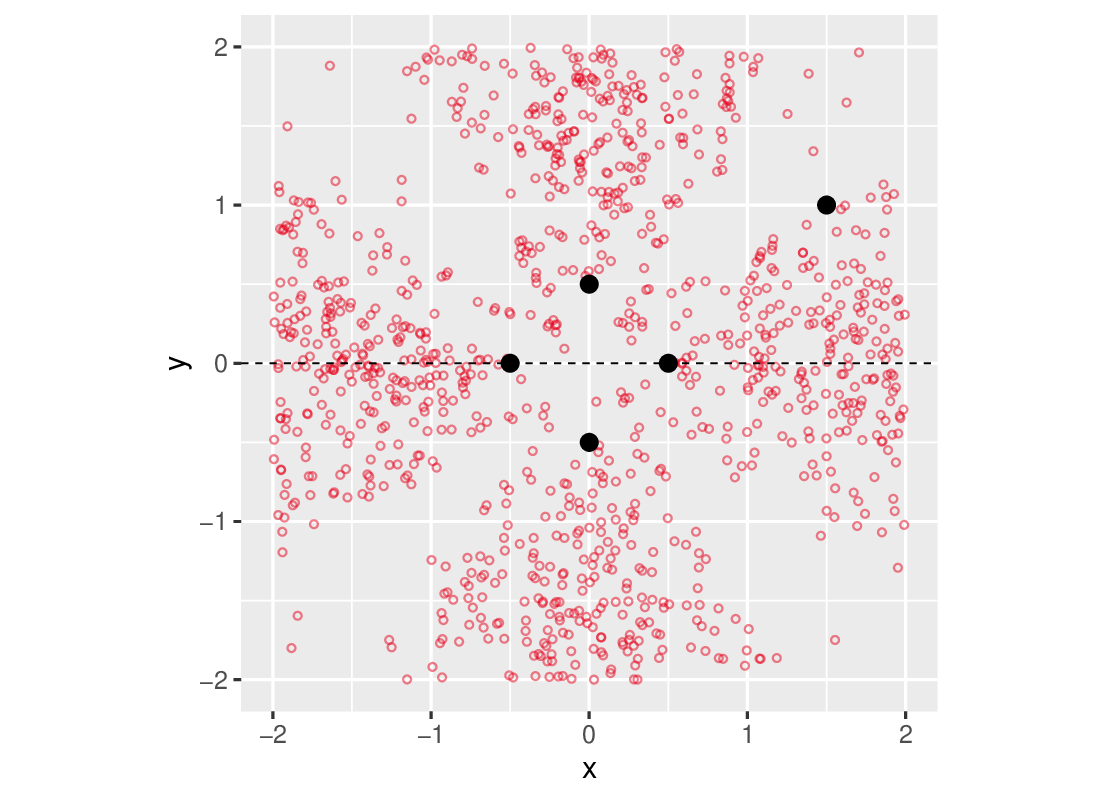
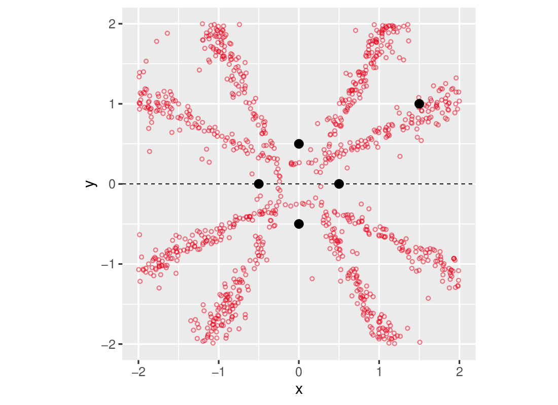
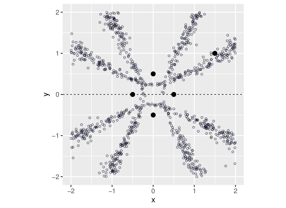
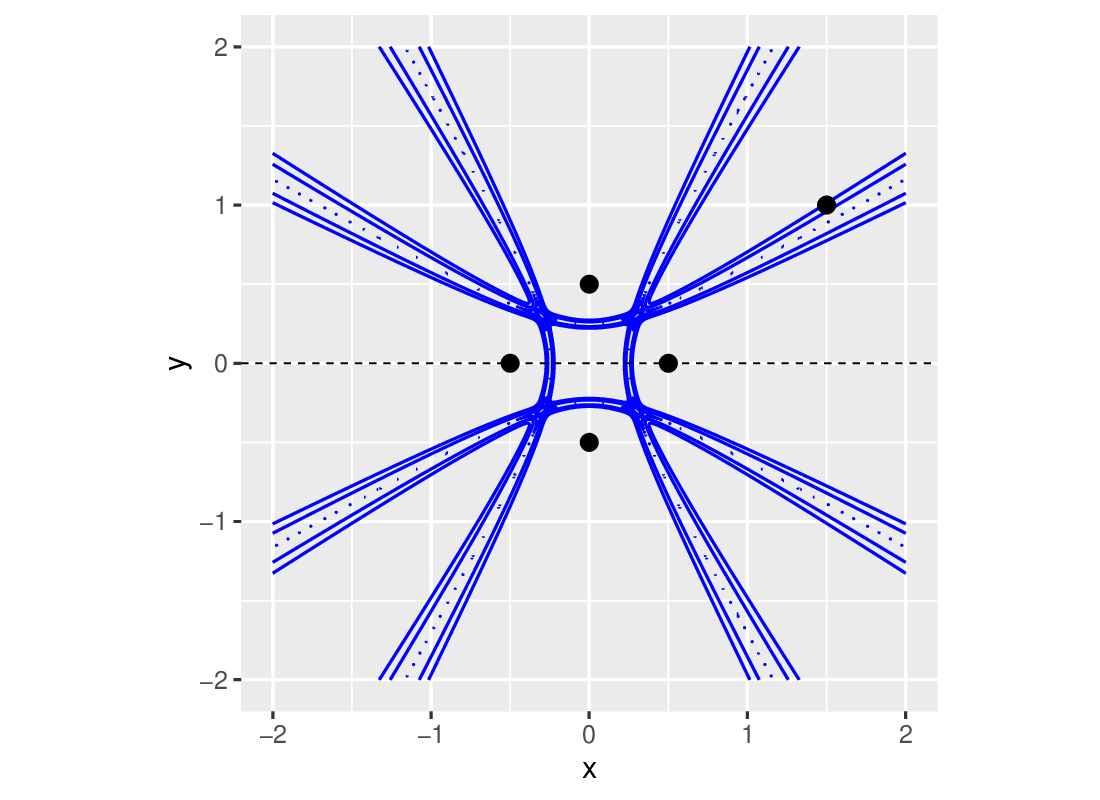
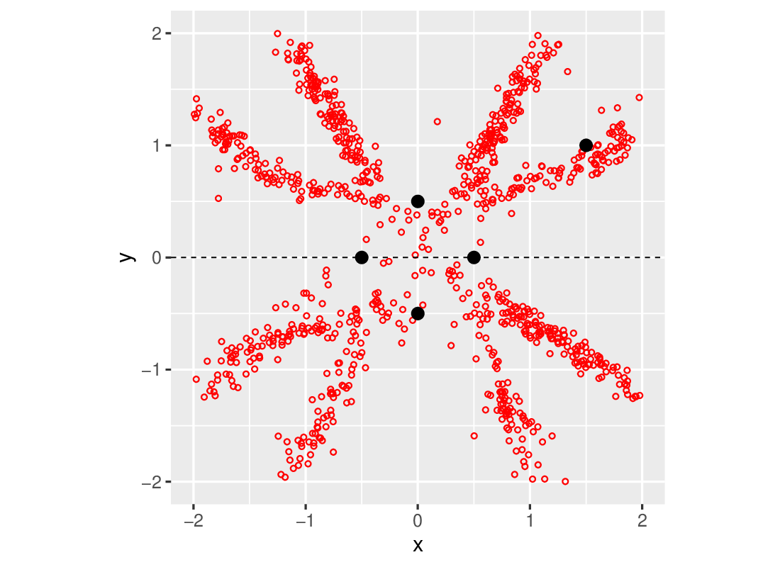
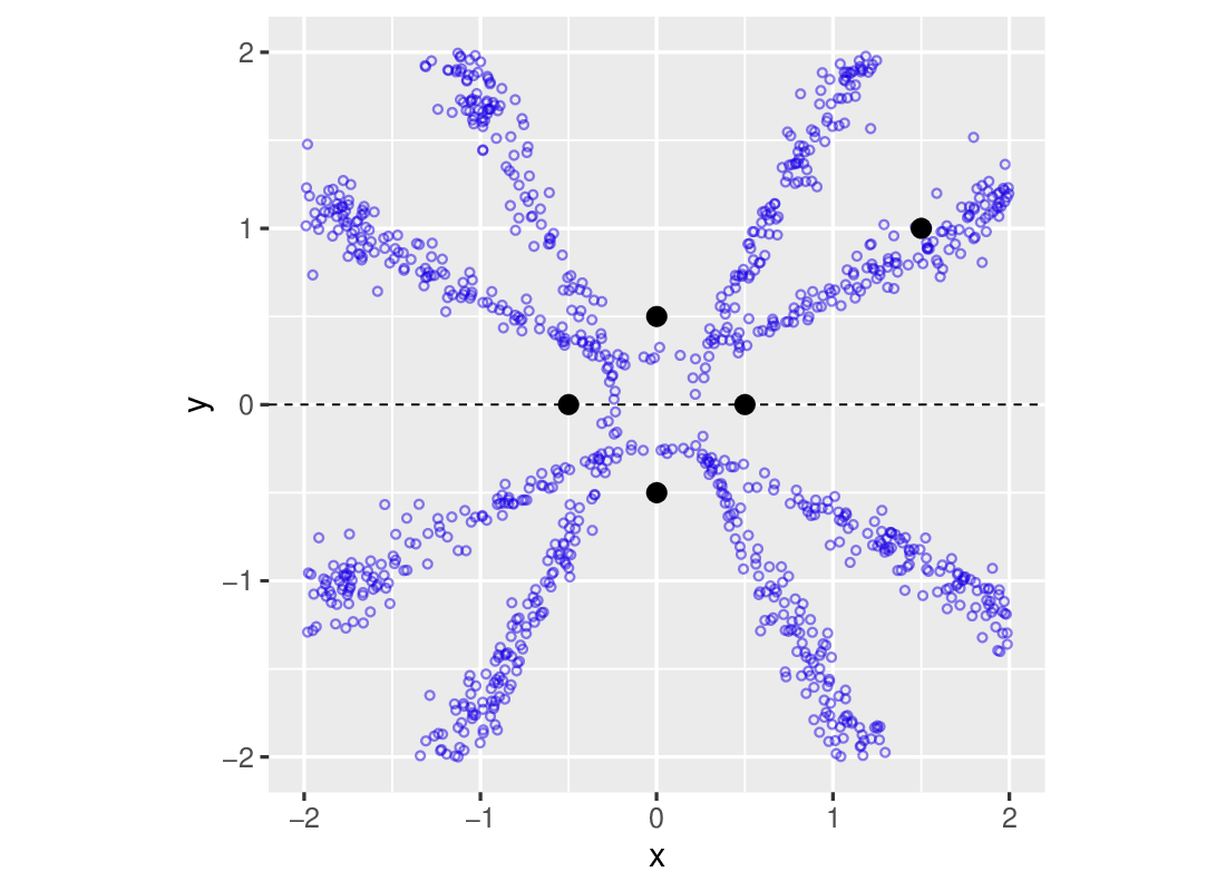
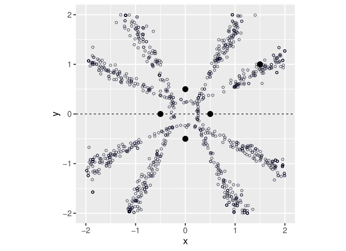
The parameter space is assumed to be $Θ = [- 2, 2] \times [- 2, 2]$ and the prior on $𝜽$ is assumed to be uniform on $Θ$ . The pair positions are $𝒎^{1} = ((- 0.5, 0), (0.5, 0))$ and $𝒎^{2} = ((0, - 0.5), (0, 0.5))$ . We assume $ν = 3$ and $σ^{2} = 0.01$ . The true $𝜽$ is set to $𝜽 = (1.5, 1)$ and we simulate a 10-dimensional $𝐲$ following model (15). Depending on whether this observation is coming from the first pair or second pair component, it results in a true posterior as shown in Figure 1 (d) or one with non-intersecting hyperbolas. The contour plot indicates that the observation corresponds to the $((0, - 0.5), (0, 0.5))$ pair. Multimodality of the posterior is coming from that each isosurface defined by (16) is represented by a two-sheet hyperboloid in 2D.

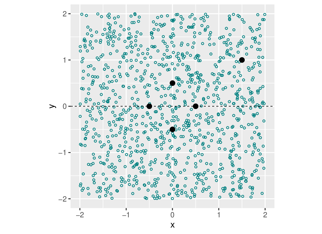
The four ABC methods using GLLiM and semi-automatic ABC are compared. The first GLLiM model used consists of $K = 20$ Gaussian components with an isotropic constraint. A selected sample of 1000 values is retained by thresholding the distances under the $0.1 %$ quantile. In a first test, semi-automatic ABC and GLLiM use the same data set of size $M = 10^{6}$ , which is also used for the rejection ABC part. Selected samples are shown in supplementary Section S4.5.2, Figure S10. The mixture provided by GLLiM as an approximation of the true posterior (Figure 10 (d)) well captures the main posterior parts. This GLLiM posterior is a $20$ -component Gaussian mixture of form (2). The true posterior expectations are all zero and are thus not informative about the location parameters. However, a correct structure can be seen in the GLLiM-E-ABC sample, in contrast to the semi-automatic one that shows no structure as expected. Adding the posterior log-variance estimations has a good impact on the selected sample, which is only marginally different from the GLLiM-D-ABC samples. This suggests that the posterior log-variances are very informative on the location parameters.

When GLLiM is first learned with a smaller data set of size $N = 10^{5}$ and different from the rejection ABC data set, results slightly degrade, but not significantly so (Supplementary Figure S11). More badly localized estimations can be seen in the samples of Figure S11 (g,h), but the GLLiM-D-ABC samples are well localized and are not really impacted by this difference in the GLLiM learning step. In this case, the improvement of GLLiM-D-ABC over GLLiM-EV-ABC is clearer.

When BIC is used to select $K$ , we observe a minimum at $K = 38$ when the criterion is computed for $K = 2$ to $K = 40$ (see supplementary Figure S12). Figure 1 below shows then the results with GLLiM learned with $K = 38$ and $N = 10^{5}$ . A clear improvement is visible, especially on the GLLiM-mixture and GLLiM-EV-ABC plots. In contrast to the MA(2) example where manually choosing $K$ too large led to similar results, choosing it too small has here more impact. We also use the better GLLiM approximation to show that the number of ABC simulations can be reduced without much changing the selected posterior samples. Plots (c) and (g) in Figure 1 are obtained by selecting among $M = 10^{5}$ simulations the best 1% distances instead of the best 0.1% in supplementary Figure S11. At last, all previously mentioned samples are obtained using a rejection ABC scheme while Figure 1 (h) is a sample obtained using the MW₂ distance and SMC-ABC. Results are very similar with a slightly better sampling with SMC at the hyperboloids intersection.

Refer to caption — Figure 1: Multiple hyperboloid example. GLLiM is learned with $K = 38$ on a data set of size $N = 10^{5}$ while ABC is run using a data set of size $M = 10^{6}$ for (a,b,f,h) and $M = 10^{5}$ for (c,g). Rejection ABC is used except for (h) which uses SMC-ABC. Selected samples using (a) GLLiM posterior expectations, (b) GLLiM posterior expectations and log variances, (c) MW₂ distances, (d) contours of the true posterior distribution, (e) approximate GLLiM posterior for the observed data, (f) semi-automatic ABC, (g) L₂ distances and (h) MW₂ distances with SMC-ABC. Black points on the dotted line are the pairs positions. The fifth black point is the true parameter value.

6.5 A physical model inversion in planetary science

As a real-world example, we consider a remote sensing application coming from the study of planetary environment; in particular, the morphological, compositional, photometrical, and textural characterization of sites on the surface of a planet. The composition of the surface materials is generally established on the basis of spectral mixing and physical modeling techniques using images produced by hyperspectral cameras, from different angles during a site flyover. An example for the planet Mars is described by Murchie et al. (2009); Fernando et al. (2016). Such observations can also be measured in the laboratory, on known materials to validate a model. In both cases, the interpretation of the surface Bidirectional Reflectance Distribution Factor (BRDF) extracted from these observations is based on the inversion of a model of radiative transfer, linking physical and observable parameters in a non-linear way.

The Hapke model is a semi-empirical photometric model that relates physically meaningful parameters to the reflectivity of a granular material for a given geometry of illumination and viewing. Formally, it links a set of parameters $𝜽 \in ℝ^{4}$ to a theoretical BRDF denoted by $𝐲 = F_{Hapke} (𝜽) \in ℝ^{d}$ . A given experiment defines $d$ geometries of measurement, each parameterized by a triplet $(θ_{0}, θ, ϕ)$ of incidence, emergence and azimuth angles. Moreover, $𝜽 = (ω, \bar{θ}, b, c)$ are the sensitive parameters, respectively single scattering albedo, macroscopic roughness, asymmetry parameter and backscattering fraction. More details on these quantities and their photometric meanings may be found in Schmidt and Fernando (2015); Labarre (2017). Although available, the expression of $F_{Hapke}$ is very complex and tedious to handle analytically, with a number of approximations required (see the description of the function in more than 15 pages in Labarre 2017). In practice, it is therefore mainly used via a numerical code, allowing simulations from the model. In addition, previous studies (Kugler et al. 2021; Schmidt and Fernando 2015) have shown evidence for the existence of multiple solutions or for the possibility to obtain very similar observations from different sets of parameters, which makes this setting appropriate for testing the ability of our procedures to recover multimodal posterior distributions.

In the following experiments, all parameters are transformed to be in $[0, 1]^{4}$ , which amounts to keep $b$ and $c$ unchanged, divide $\bar{θ}$ by 30 and operate the following change of variable for $ω$ , $γ = 1 - \sqrt{1 - ω}$ . This last transformation also has the advantage of avoiding the non-linearity of $F_{Hapke}$ , when $ω$ tends to 1. The experimental setting defines geometries at which the measurements are made, which in turn define $F_{Hapke}$ . The number of geometries thus corresponds to the size $d$ , of each observation. The measurement geometries used to define $F_{Hapke}$ are borrowed from a real laboratory experiment presented below. The number of parameters is therefore $ℓ = 4$ with $d = 10$ observed geometries. The sets to learn GLLiM and generate ABC samples are both set to size $N = M = 10^{5}$ . For each pair $(𝜽, 𝐲)$ in the simulated data sets, the $4$ parameters ( $𝜽$ ) are simulated uniformly in $[0, 1]^{4}$ . Besides these learning sets, the Hapke simulator is not available to us so we cannot run SMC-ABC for this specific example. Following a previous study (Kugler et al., 2021), the corresponding reflectance curves are generated as $𝐲 = F_{Hapke} (𝜽) + 𝜺$ , where $𝜺$ is a centered Gaussian variable with isotropic covariance $σ^{2} I_{d}$ . In this section $σ = 0.05$ . The GLLiM model is learned with $K = 40$ to be consistent with a previous study (Kugler et al., 2021). We check that this value is reasonable and in particular that it cannot be significantly reduced. BIC is computed from $K = 2$ to $K = 40$ . The BIC values are shown in supplementary Figure S13. The minimum is reached for $K = 39$ but $K = 40$ provides almost the same BIC.

Prior to real data inversion, performance is assessed by considering an observation simulated from the Hapke model, as explained in the supplementary Section S4.6.2. In this experiment, $ϵ$ is varying to observe the behavior of the different methods (Figure S14). GLLiM-L2-ABC seems less robust, than the other procedures, to these variations and even degrades in performance when $ϵ$ is too high. The two procedures based on expectations show satisfying performance with globally less sharp posteriors. The addition of the posterior log-variances does not seem to significantly change the selected samples.

Reflectance measurements made in the laboratory are also generally considered by experts (see e.g. Pilorget et al. 2016). We focus on one observation coming from a mineral called Nontronite (see Kugler et al. 2021 for a description). The experiment consists of taking measures at 100 wavelengths in the spectral range 400–2800 nm. Each of these 100 measures is an observation to be inverted. We focus on one of them, at 2310 nm. This observation has been chosen from previous study (Kugler et al., 2021) as likely to exhibit multiple solutions. The size $d$ of each observation is $d = 10$ and the corresponding angles are such that the incidence and azimuth angles are fixed to $θ_{0} = 45$ and $ϕ = 0$ . This number $d$ of geometries is typical of real observations for which the number of possible measurements during a planet flyover is limited.

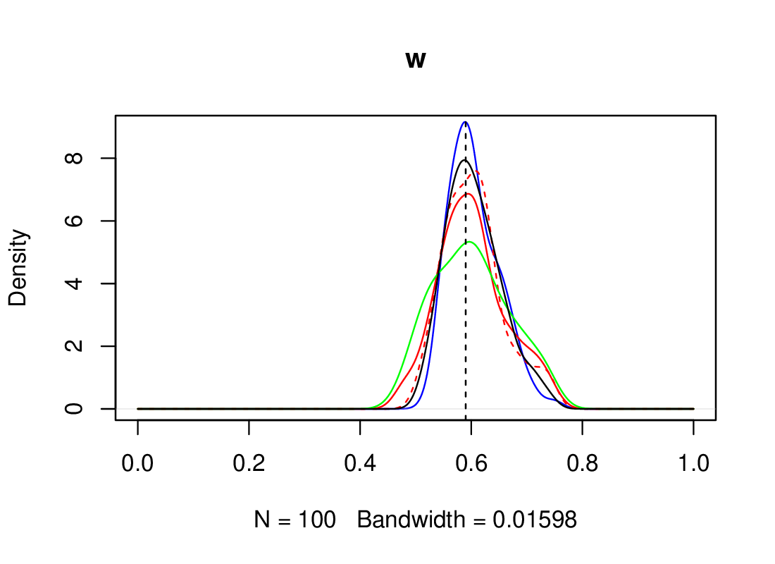
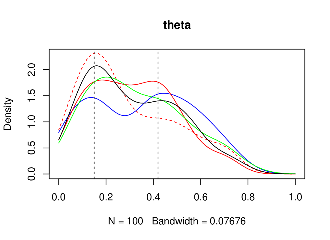
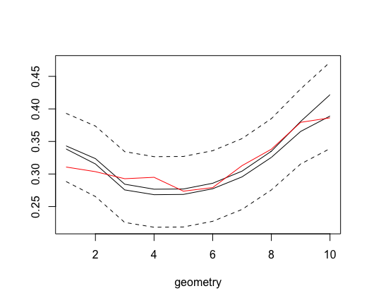
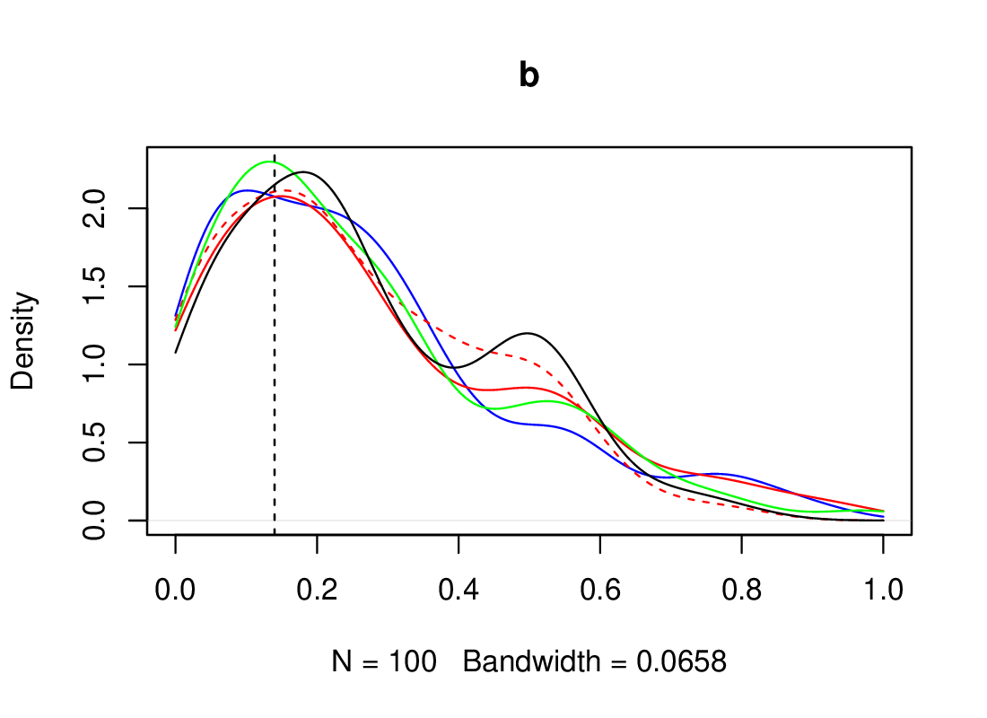
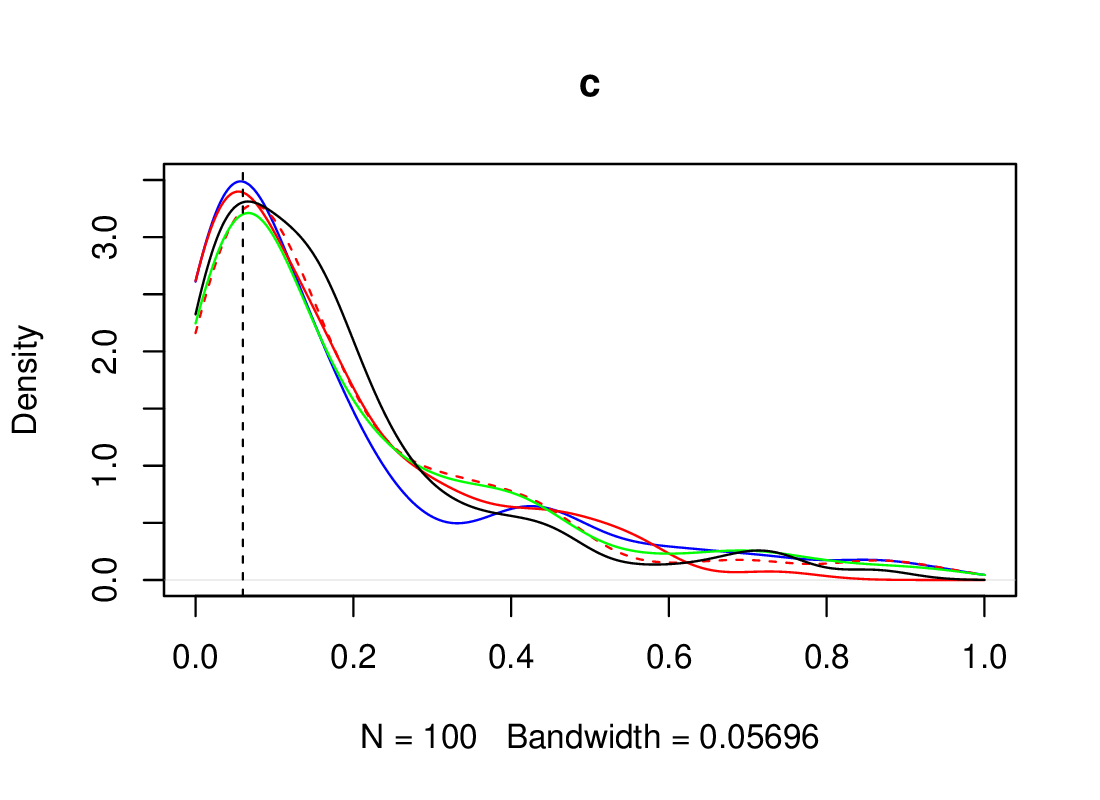
Figure 2 provides the posterior marginals for the Nontronite, obtained by setting $ϵ$ to the 0.1% quantile of the distances. Two solutions can be deduced. Parameters $ω$ and $c$ show unimodal posterior distributions, while $\bar{θ}$ distribution exhibits two modes. For $b$ , the GLLiM-MW2-ABC sample shows a second smaller mode around 0.5 but this mode is not maintained when $ϵ$ is set to a lower quantile (see Figure S15 in supplementary Section S4.6.3). We therefore consider that the multiplicity comes mainly from $\bar{θ}$ . In the absence of ground truth, it is difficult to fully validate the estimations. However a simple inspection consists of checking the reconstructed signals. The top-right plot in Figure 2 compares the inverted signal to the reconstructed signals obtained by applying the Hapke model to the two sets of estimated parameters, namely $(0.59, 0.15, 0.14, 0.06)$ and $(0.59, 0.42, 0.14, 0.06)$ , which differ only in $\bar{θ}$ . The proximity of the reconstructions confirms the existence of multiple solutions and thus the relevance of a multimodal posterior. One solution can be selected by choosing the parameters that provide the best reconstruction. The set $(0.59, 0.42, 0.14, 0.06)$ is selected as its MSE is slightly lower ( $2.6 \times 10^{- 4}$ vs $3.3 \times 10^{- 4}$ ). This is satisfactory, as the lower value of $\bar{θ}$ in the other solution is less physically interpretable. Note that for simplicity, we have used a uniform prior on $𝜽$ but for a more meaningful study in planetary science, information on the parameters’ plausible values could be incorporated directly in the prior.

6.6 Computation times

The simulations ran on a laptop with 8 cores at 2.4 Ghz. Supplementary Table S3 recalls the settings and shows the computation times for the main experiments. For each experiment, the time is divided into several parts depending on the procedure. When GLLiM is used, we report the time to compute BIC from $K = 2$ to some $K_{m a x}$ value, the time for learning GLLiM with the selected $K$ value, the time to compute distances, and the time for the ABC procedure per se, which consists either of rejection ABC or SMC-ABC. In the latter case, the computation of the distances is included in the ABC time. The compared procedures use different R packages. The computing times are therefore not fully comparable. However the overall conclusions are quite clear. The semi-automatic approach as implemented in the abctools package is much faster than any other tested procedure. When dimensions of both observations and parameters are moderate and posterior distributions are likely to be unimodal, semi-automatic ABC is the most efficient choice. In contrast, GLLiM-based approaches are much more costly, especially if we include the time spent in selecting $K$ via BIC. SMC-ABC is in general more efficient than rejection ABC even when the number of simulations is similar (see the MA(2) case). We suspect this is due to a better implementation and memory usage in the winference package compared to our code. The GLLiM implementation could certainly be improved but would remain based on an EM algorithm, which is intrinsically slower, although one interesting investigation would be to consider stochastic, incremental, or online EM algorithm implementations (see e.g. Cappé and Moulines (2009); Nguyen et al. (2020a); Nguyen and Forbes (2022)) for better computing time and memory usage. When EM is not used, as in the very special case of the normal location model, GLLiM-D-SMC procedures are actually much faster (1 to 2 minutes) vs. 50 minutes for WABC, which is blind to the parametric structure of the model. GLLiM-based procedures also show quite different timings depending on the experiments, ranging from a few minutes to several hours. This is due to the different GLLiM implementations (e.g. GLLiM-iid vs standard GLLiM) and learning sets sizes and dimensions. The number of components $K$ has also an impact on the cost of each GLLiM iteration and reflects the model complexity. For example, the Bivariate Beta model is learned with $K = 100$ in about 11 hours, which is an extreme case. We suspect this is due to the difficulty in fitting such a model. More iterations are needed for EM to converge and each iteration has a higher cost. For comparison learning GLLiM on the 14 quantiles summaries and $K = 40$ takes about 10 minutes. Reversely, the cost of computing L₂ or MW₂ distances may vary surprisingly for models of similar dimensions. The Wasserstein distance cost increases with the dimension and the number of components in the mixture. In practice, we propose to accelerate this computation by neglecting components with too low weights. This can be quite efficient in the unimodal posterior case (1 minute 3 seconds for the MW₂ distances in the MA(2) example), while in the multiple hyperboloid example (4 hours 18 minutes for the MW₂ distances), most mixtures contain 8 components, one for each "branch", and cannot be reduced. We refer to supplementary Section S5 for more detailed comments.

7 Conclusion and perspectives

In this work, the issue of choosing summary statistics was revisited. We built on the seminal work of Fearnhead and Prangle (2012) and their semi-automatic ABC by replacing the approximate posterior expectations with functional statistics; namely approximations of the posterior distributions. These surrogate posterior distributions were obtained in a preliminary learning step, based on an inverse regression principle. This is original with respect to most standard regression procedures, which usually provide only point-wise predictions, i.e. first-order moments. So doing, we not only could compute approximate posterior moments of higher orders as summary statistics but, more generally, approximate full posterior distributions. This learning step was based on the so-called GLLiM model, which provides surrogate posteriors in the parametric family of Gaussian mixtures. Preliminary experiments showed that although the posterior moments provided by GLLiM were not always leading to better results than that provided by semi-automatic ABC, the use of the full surrogate posteriors was always an improvement. Consequently, an interesting feature of our approach is that, with our adaptation of the original GLLiM model to i.i.d. data, it can be seen as an alternative to both summary-based and discrepancy-based procedures.

To handle distributions as functional summary statistics, our procedure required appropriate distances. We investigated an L₂ and a Wasserstein-based distance (MW₂). The two distances often performed similarly but poor results have been observed with L₂ that would require further investigations. The MW₂ distance appeared to be more robust. As illustrated in our remote sensing example, it may also allow for the ability to set the tolerance level at a higher value without overly degrading the quality of the posterior sample.

Among aspects that have not been thoroughly investigated in this work, we could refine the way to choose this tolerance level $ϵ$ or combine GLLiM with more sophisticated ABC schemes than the simple rejection scheme.

Another interesting perspective would be to investigate the use of GLLiM in the context of synthetic likelihood (SL) approaches. When used in a Bayesian framework, SL techniques can be viewed as alternatives to ABC in which the intractable likelihood is replaced by an estimator of the likelihood (Price et al., 2018). Since the seminal work of Wood (2010), several estimators have been proposed (e.g. Ong et al., 2018; An et al., 2019, 2020; Frazier and Drovandi, 2021), often derived from auxiliary models (Drovandi et al., 2015). In the ABC framework of this paper, GLLiM was used to provide approximate posteriors but these posteriors are themselves coming from approximate likelihoods that could lead to new SL procedures.

Lastly, in principle, any other method that is able to provide approximate surrogate posteriors could be used in place of GLLiM to produce the functional summaries. Besides the family of mixture of experts models which are similar to GLLiM, mixture density networks (Bishop, 1994) or normalizing flows (Dinh et al., 2015; Kobyzev et al., 2020; Kruse et al., 2021) are potential candidates. These neural networks have already been used in likelihood-free inference to directly approximate likelihoods or posteriors. The corresponding approaches are related to Sequential Neural Posterior Estimation (SNPE) and are different from our approach in that the approximate posteriors are not used to compute distances in a subsequent ABC scheme. SNPE is a strategy for reducing the number of simulations needed by conditional neural density estimation and is closer in spirit to SMC-ABC. These methods include SNPE-A (Papamakarios and Murray, 2016), SNPE-B (Lueckmann et al., 2017), SNPE-C or AFT (Greenberg et al., 2019). However, these methods do not all scale well with the dimension. Examples of Papamakarios and Murray (2016) are of dimension at most 10, while SNPE-C is used successfully on Lokta-Volterra time series of length 150. Overall, it is not clear whether the gain/compromise in flexibility/tractability would be so much higher than with Gaussian mixtures learned with GLLiM, all the more so as GLLiM estimation could also be refined in a similar sequential learning way. A full and fair comparison would require much more work as these methods have all their own features. To the best of our knowledge, other common neural networks, like most regression techniques, would not be appropriate as they only focus on point-wise predictions.

Acknowledgements.

The authors are grateful to reviewers and editors for their time and comments on this work, which have helped us in producing a much-improved manuscript. FF would like to thank Guillaume Kon Kam King for an initial discussion on semi-automatic ABC, which inspired this work, Benoît Kugler and Sylvain Douté for providing the simulations for the planetary science example, and for helpful discussions on the Hapke model. The work is supported by Inria project LANDER.

References

M. Akesson, P. Singh, F. Wrede, and A. Hellander (2021) Convolutional Neural Networks as Summary Statistics for Approximate Bayesian Computation. IEEE/ACM Transactions on Computational Biology and Bioinformatics. Cited by: §1, §4. ↩ a b
Z. An, D. J. Nott, and C. Drovandi (2020) Robust Bayesian synthetic likelihood via a semi-parametric approach. Statistics and Computing 30 (3), pp. 543–557. External Links: ISSN 1573-1375, Link, Document Cited by: §7. ↩ a
Z. An, L. F. South, D. J. Nott, and C. C. Drovandi (2019) Accelerating Bayesian Synthetic Likelihood With the Graphical Lasso. Journal of Computational and Graphical Statistics 28 (2), pp. 471–475. Note: Publisher: Taylor & Francisdoi: 10.1080/10618600.2018.1537928 External Links: ISSN 1061-8600, Link, Document Cited by: §7. ↩ a
S. Arridge, P. Maass, O. Öktem, and C. Schönlieb (2019) Solving inverse problems using data-driven models. Acta Numerica 28, pp. 1–174 (en). External Links: ISSN 0962–4929, 1474–0508 Cited by: §3. ↩ a
C. Bernard-Michel, S. Douté, M. Fauvel, L. Gardes, and S. Girard (2009) Retrieval of Mars surface physical properties from OMEGA hyperspectral images using Regularized Sliced Inverse Regression. Journal of Geophysical Research: Planets 114 (E6). Cited by: §1. ↩ a b
E. Bernton, P. E. Jacob, M. Gerber, and C. P. Robert (2019) Approximate Bayesian computation with the Wasserstein distance. Journal of the Royal Statistical Society: Series B (Statistical Methodology) 81, pp. 235–269. Cited by: §1, §1, §2, §2, §5.1, §5.1, §6.1, §6.2.1, §6.2.2, §6.2, §6.3, §6. ↩ a b c d e f g h i j k l m n o p q r s
C. M. Bishop (1994) Mixture density networks. Technical report Aston University, Birmingham. Cited by: §3, §7. ↩ a b
M. G. B. Blum, M. A. Nunes, D. Prangle, and S. A. Sisson (2013) A comparative review of dimension reduction methods in approximate Bayesian computation. Statistical Science 28 (2), pp. 189–208. Cited by: §1. ↩ a
F. Boux, F. Forbes, J. Arbel, B. Lemasson, and E. L. Barbier (2021) Bayesian Inverse Regression for Vascular Magnetic Resonance Fingerprinting. IEEE Trans. Medical Imaging 40 (7), pp. 1827–1837. Cited by: §3. ↩ a
A. Buchholz and N. Chopin (2019) Improving Approximate Bayesian Computation via Quasi-Monte Carlo. Journal of Computational and Graphical Statistics 28 (1), pp. 205–219. Cited by: §1. ↩ a
O. Cappé and E. Moulines (2009) On-line expectation-maximization algorithm for latent data models. Journal of the Royal Statistical Society B 71, pp. 593–613. Cited by: §6.6. ↩ a
Y. Chen, T. T. Georgiou, and A. Tannenbaum (2019) Optimal Transport for Gaussian Mixture Models. IEEE Access 7, pp. 6269–6278. Cited by: §1, §2, §4.2. ↩ a b c
Y. Chen, D. Zhang, M. Gutmann, A. Courville, and Z. Zhu (2021) Neural Approximate Sufficient Statistics for Implicit Models. In ICLR2021 spotlight, Cited by: §1, §4.1. ↩ a b c
R. D. Cook and L. Forzani (2019) Partial least squares prediction in high-dimensional regression. The Annals of Statistics 47 (2), pp. 884–908 (EN). External Links: ISSN 0090-5364, 2168-8966, MathReview Entry Cited by: §3. ↩ a
R. Crackel and J. Flegal (2017) Bayesian inference for a flexible class of bivariate beta distributions. Journal of Statistical Computation and Simulation 87, pp. 295–312. Cited by: §6.2, §6.2. ↩ a b
K. Csillery, O. Francois, and M. Blum (2012) abc: an R package for approximate Bayesian computation (ABC). Methods in Ecology and Evolution. Cited by: §6. ↩ a
P. Del Moral, A. Doucet, and A. Jasra (2012) An Adaptive Sequential Monte Carlo Method for Approximate Bayesian Computation. Statistics and Computing 22 (5), pp. 1009–1020. Cited by: §1. ↩ a
A. Deleforge, F. Forbes, S. Ba, and R. Horaud (2015a) Hyper-Spectral Image Analysis with Partially-Latent Regression and Spatial Markov Dependencies. IEEE Journal of Selected Topics in Signal Processing 9 (6), pp. 1037–1048. Cited by: §1. ↩ a
A. Deleforge, F. Forbes, and R. Horaud (2015b) High-Dimensional Regression with Gaussian Mixtures and Partially-Latent Response Variables. Statistics and Computing 25 (5), pp. 893–911. Cited by: §1, §3, §3, §3, §4.2, §6. ↩ a b c d e f g h
J. Delon and A. Desolneux (2020) A Wasserstein-type distance in the space of Gaussian Mixture Models. SIAM Journal on Imaging Sciences. Cited by: §1, §2, §4.2. ↩ a b c d
L. Dinh, D. Krueger, and Y. Bengio (2015) NICE: non-linear independent components estimation. In 3rd International Conference on Learning Representations, ICLR 2015, San Diego, CA, USA, May 7-9, 2015, Workshop Track Proceedings, Y. Bengio and Y. LeCun (Eds.), Cited by: §3, §7. ↩ a b
C. C. Drovandi and A. N. Pettitt (2011) Likelihood-free Bayesian estimation of multivariate quantile distributions. Computational Statistics and Data Analysis 55, pp. 2541–2556. Cited by: §1. ↩ a
C. Drovandi, T. Pettitt, and A. Lee (2015) Bayesian indirect inference using a parametric auxiliary model. Statistical Science 30 (1), pp. 72–95. Cited by: §7. ↩ a
P. Fearnhead and D. Prangle (2012) Constructing summary statistics for approximate Bayesian computation: semi-automatic approximate Bayesian computation. Journal of the Royal Statistical Society: Series B (Statistical Methodology) 74 (3), pp. 419–474. Cited by: §1, §1, §1, §2, §3, §4, §6.2.1, §6.3, §6, §7. ↩ a b c d e f g h i j k
J. Fernando, F. Schmidt, and S. Douté (2016) Martian surface microtexture from orbital CRISM multi-angular observations: A new perspective for the characterization of the geological processes. Planetary and Space Science 128, pp. 30–51. Cited by: §6.5. ↩ a
D. T. Frazier and C. Drovandi (2021) Robust Approximate Bayesian Inference With Synthetic Likelihood. Journal of Computational and Graphical Statistics, pp. 1–19. Cited by: §7. ↩ a
D. Greenberg, M. Nonnenmacher, and J. Macke (2019) Automatic posterior transformation for likelihood-free inference. In International Conference on Machine Learning, pp. 2404–2414. Cited by: §7. ↩ a
M. U. Gutmann, R. Dutta, S. Kaski, and J. Corander (2018) Likelihood-free inference via classification. Statistics and Computing 28, pp. 411–425. Cited by: §1, §2, §2. ↩ a b c d
R. Hovorka, V. Canonico, L. J. Chassin, U. Haueter, M. Massi-Benedetti, M. O. Federici, T. R. Pieber, H. C. Schaller, L. Schaupp, T. Vering, and M. E. Wilinska (2004) Nonlinear model predictive control of glucose concentration in subjects with type 1 diabetes. Physiological Measurement 25 (4), pp. 905–920. Cited by: §1. ↩ a
S. Ingrassia, S. C. Minotti, and G. Vittadini (2012) Local Statistical Modeling via a Cluster-Weighted Approach with Elliptical Distributions. Journal of classification 29 (3), pp. 363–401. Cited by: §3. ↩ a
P. Jacob, E. Bernton, M. Gerber, and C. P. Robert (2020) Winference: R package to perform approximate Bayesian computation with the Wasserstein distance. External Links: Link Cited by: §6. ↩ a
B. Jiang, T-Y. Wu, Z. C., and W.H. Wong (2017) Learning summary statistics for Approximate Bayesian Computation via Deep Neural Network. Statistica Sinica, pp. 1595–1618. Cited by: §1, §1, §3, §4, §6.2.1, §6.3, §6.3, §6.3, Table 2, §6. ↩ a b c d e f g h i j k l m n o
B. Jiang, T-Y. Wu, and W. H. Wong (2018) Approximate Bayesian computation with Kullback-Leibler divergence as data discrepancy. In 21st International Conference on Artificial Intelligence and Statistics (AISTATS), Cited by: §2, §2, §6.2.1, §6.2.1, §6.2.1, §6.2, §6.2, §6.3. ↩ a b c d e f g h i
I. Kobyzev, S. Prince, and M. Brubaker (2020) Normalizing Flows: An Introduction and Review of Current Methods. IEEE Trans. Pattern Anal. Mach. Intell., pp. 1–1. External Links: Link Cited by: §7. ↩ a
M. Kristan, A. Leonardis, and D. Skočaj (2011) Multivariate online kernel density estimation with Gaussian kernels. Pattern Recognition 44 (10-11), pp. 2630–2642. Cited by: §2. ↩ a
J. Kruse, L. Ardizzone, C. Rother, and U. Kothe (2021) Benchmarking invertible architectures on inverse problems. Workshop on Invertible Neural Networks and Normalizing Flows (ICML 2019), arXiv preprint arXiv:2101.10763. Cited by: §7. ↩ a
B. Kugler, F. Forbes, and S. Douté (2021) Fast Bayesian Inversion for high dimensional inverse problems. To appear in Statistics and Computing, https://hal.archives-ouvertes.fr/hal-02908364. Cited by: §6.5, §6.5, §6.5. ↩ a b c d e
S. Labarre (2017) Caractérisation et modélisation de la rugosité multi-échelle des surfaces naturelles par télédétection dans le domaine solaire. Ph.D. Thesis, Physique Univers Sorbonne Paris Cité. Note: Supervised by C. Ferrari and S. Jacquemoud External Links: Link Cited by: §6.5. ↩ a b
B. Lemasson, N. Pannetier, N. Coquery, L. S. B. Boisserand, N. Collomb, N. Schuff, M. Moseley, G. Zaharchuk, E. L. Barbier, and T. Christen (2016) MR Vascular Fingerprinting in Stroke and Brain Tumors Models. Scientific Reports 6, pp. 37071 (en). External Links: ISSN 2045-2322 Cited by: §1. ↩ a
K. Li (1991) Sliced Inverse Regression for Dimension Reduction. Journal of American Statistical Association 86 (414), pp. 316–327. External Links: ISSN 0162-1459 Cited by: §3. ↩ a
J.-M. Lueckmann, J. Boelts, D. S. Greenberg, P. J. GonÃ§alves, and J. H. Macke (2021) Benchmarking simulation-based inference. In Proceedings of the 24th International Conference on Artificial Intelligence and Statistics (AISTATS), Proceedings of Machine Learning Research, Vol. 130, pp. 343–351. Cited by: §6.2. ↩ a
J. Lueckmann, P. J. Goncalves, G. Bassetto, K. Öcal, M. Nonnenmacher, and J. H. Macke (2017) Flexible statistical inference for mechanistic models of neural dynamics. In Advances in Neural Information Processing Systems, I. Guyon, U. V. Luxburg, S. Bengio, H. Wallach, R. Fergus, S. Vishwanathan, and R. Garnett (Eds.), Vol. 30, pp. . Cited by: §7. ↩ a
D. Ma, V. Gulani, N. Seiberlich, K. Liu, J. L. Sunshine, J. L. Duerk, and M. A. Griswold (2013) Magnetic Resonance Fingerprinting. Nature 495 (7440), pp. 187–192. External Links: ISSN 0028-0836 Cited by: §1. ↩ a
J-M. Marin, P. Pudlo, C. P. Robert, and R. J. Ryder (2012) Approximate Bayesian computation methods. Statistics and Computing 22, pp. 1167–1180. Cited by: §6.3. ↩ a
P. Mesejo, S. Saillet, O. David, C. Bénar, J. M. Warnking, and F. Forbes (2016) A differential evolution-based approach for fitting a nonlinear biophysical model to fMRI BOLD data. IEEE Journal of Selected Topics in Signal Processing 10 (2), pp. 416–427. Cited by: §1. ↩ a
K. Muandet, K. Fukumizu, F. Dinuzzo, and B. Scholkopf (2012) Learning from distributions via support measure machines. In Advances in Neural Information Processing Systems, pp. 10–18. Cited by: §2. ↩ a
S. L. Murchie, F. P. Seelos, C. D. Hash, D. C. Humm, E. Malaret, J. A. McGovern, T. H. Choo, K. D. Seelos, D. L. Buczkowski, M. F. Morgan, O. S. Barnouin-Jha, H. Nair, H. W. Taylor, G. W. Patterson, C. A. Harvel, J. F. Mustard, R. E. Arvidson, P. McGuire, M. D. Smith, M. J. Wolff, T. N. Titus, J. Bibring, and F. Poulet (2009) Compact Reconnaissance Imaging Spectrometer for Mars investigation and data set from the Mars Reconnaissance Orbiter’s primary science phase. Journal of Geophysical Research: Planets 114 (E2), pp. E00D07 (en). Cited by: §6.5. ↩ a
G. Nataraj, J. Nielsen, C. Scott, and J. A. Fessler (2018) Dictionary-Free MRI PERK: Parameter Estimation via Regression with Kernels. IEEE Trans. Med. Imaging 37 (9), pp. 2103–2114. External Links: ISSN 1558-254X Cited by: §3. ↩ a
H. D. Nguyen, F. Forbes, and G.J. McLachlan (2020a) Mini-batch learning of exponential family finite mixture models. Statistics and Computing 30, pp. 731–748. Cited by: §6.6. ↩ a
H.D. Nguyen and F. Forbes (2022) Global implicit function theorems and the online expectation–maximisation algorithm. Australian and New Zealand Journal of Statistics to appear. Cited by: §6.6. ↩ a
H. D. Nguyen, F. Chamroukhi, and F. Forbes (2019) Approximation results regarding the multiple-output Gaussian gated mixture of linear experts model. Neurocomputing. External Links: ISSN 0925-2312 Cited by: §3, §3. ↩ a b c
H. D. Nguyen, J. Arbel, H. Lu, and F. Forbes (2020b) Approximate Bayesian Computation Via the Energy Statistic. IEEE Access 8, pp. 131683–131698. External Links: ISSN 2169-3536, Document Cited by: §1, §2, §2, §4.2, §6.2.1, §6.2.1, §6.2.1, §6.2.1, §6.2, §6.2, §6.3, Table 1, §6. ↩ a b c d e f g h i j k l m n o p
H. D. Nguyen, T. Nguyen, F. Chamroukhi, and G. J. McLachlan (2021) Approximations of conditional probability density functions in Lebesgue spaces via mixture of experts models. Journal of Statistical Distributions and Applications 8 (1), pp. 13. External Links: ISSN 2195-5832, Link Cited by: §3, §3. ↩ a b
T. Nguyen, F. Chamroukhi, H. D. Nguyen, and G. J. McLachlan (2022a) Approximation of probability density functions via location-scale finite mixtures in Lebesgue spaces. Communications in Statistics - Theory and Methods, pp. 1–12. Cited by: §3. ↩ a
T. Nguyen, H. D. Nguyen, F. Chamroukhi, and G. J. McLachlan (2020c) Approximation by finite mixtures of continuous density functions that vanish at infinity. Cogent Mathematics & Statistics 7 (1), pp. 1750861. Cited by: §3. ↩ a
T. Nguyen, H. D. Nguyen, F. Chamroukhi, and F. Forbes (2022b) A non-asymptotic approach for model selection via penalization in high-dimensional mixture of experts models. To appear in Electronic Journal of Statistics. External Links: 2104.02640, Link Cited by: §3. ↩ a
M. A. Nunes and D. Prangle (2015) Abctools: an R package for tuning Approximate Bayesian Computation analyses. Note: https://cran.r-project.org/web/packages/abctools/ Cited by: §6. ↩ a
V. Ong, D. Nott, M. Tran, S. Sisson, and C. Drovandi (2018) Likelihood-free inference in high dimensions with synthetic likelihood. Computational Statistics and Data Analysis 128. Cited by: §7. ↩ a
G. Papamakarios and I. Murray (2016) Fast $ε$ -Free Inference of Simulation Models with Bayesian Conditional Density Estimation. In Advances in Neural Information Processing Systems, D. Lee, M. Sugiyama, U. Luxburg, I. Guyon, and R. Garnett (Eds.), Vol. 29. External Links: Link Cited by: §7. ↩ a b
M. Park, W. Jitkrittum, and D. Sejdinovic (2016) K2-ABC: approximate Bayesian computation with kernel embeddings. In 19th International Conference on Artificial Intelligence and Statistics (AISTATS), Cited by: §2, §2. ↩ a b
E. Perthame, F. Forbes, A. Deleforge, E. Devijver, and M. Gallopin (2017) xLLiM: High Dimensional Locally-Linear Mapping. Note: R package version 2.1 External Links: Link Cited by: §6. ↩ a
C. Pilorget, J. Fernando, B. L. Ehlmann, F. Schmidt, and T. Hiroi (2016) Wavelength dependence of scattering properties in the VIS–NIR and links with grain-scale physical and compositional properties. Icarus 267, pp. 296–314. Cited by: §6.5. ↩ a
D. Prangle, R. G. Everitt, and T. Kypraios (2018) A rare event approach to high-dimensional approximate Bayesian computation. Statistics and Computing 28, pp. 819–834. Cited by: §5.1. ↩ a
D. Prangle (2017) Adapting the ABC Distance Function. Bayesian Analysis 12 (1), pp. 289 – 309. Cited by: §1. ↩ a
L. F. Price, C. C. Drovandi, A. Lee, and D. J. Nott (2018) Bayesian Synthetic Likelihood. Journal of Computational and Graphical Statistics 27 (1), pp. 1–11. Cited by: §7. ↩ a
A. Rakhlin, D. Panchenko, and S. Mukherjee (2005) Risk bounds for mixture density estimation. ESAIM: Probability and Statistics 9, pp. 220–229. Cited by: §5.2, §5.2. ↩ a b
G. S. Rodrigues, D. J. Nott, and S. A. Sisson (2016) Functional regression approximate Bayesian computation for Gaussian process density estimation. Computational Statistics & Data Analysis 103, pp. 229–241. External Links: ISSN 0167-9473, Link, Document Cited by: §2. ↩ a b
F. Rubio and A. M. Johansen (2013) A simple approach to maximum intractable likelihood estimation. Electronic Journal of Statistics 7, pp. 1632–1654. Cited by: §5.1. ↩ a
F. Schmidt and J. Fernando (2015) Realistic uncertainties on Hapke model parameters from photometric measurements. Icarus 260, pp. 73–93. Cited by: §1, §6.5. ↩ a b c
S. A. Sisson, Y. Fan, and M. A. Beaumont (Eds.) (2019) Handbook of Approximate Bayesian Computation. CRC Press, Boca Raton. Cited by: §1. ↩ a
S. Soubeyrand, F. Carpentier, F. Guiton, and E. K. Klein (2013) Approximate Bayesian computation with functional statistics. Statistical Applications in Genetics and Molecular Biology 12 (1), pp. 17–37. Cited by: §2. ↩ a
B. K. Sriperumbudur, A. Gretton, K. Fukumizu, B. Scholkopf, and G. R. Lanckriet (2010) Hilbert space embeddings and metrics on probability measures. The Journal of Machine Learning Research 11, pp. 1517–1561. Cited by: §2. ↩ a
F. Wang, T. Syeda-Mahmood, B. C. Vemuri, D. Beymer, and A. Rangarajan (2009) Closed-form Jensen-Renyi divergence for mixture of Gaussians and applications to group-wise shape registration. In International Conference on Medical Image Computing and Computer-Assisted Intervention, pp. 648–655. Cited by: §2. ↩ a
S. Wiqvist, P.-A. Mattei, U. Picchini, and J. Frellsen (2019) Partially exchangeable networks and architectures for learning summary statistics in approximate Bayesian computation. In Proceedings of the 36th International Conference on Machine Learning, K. Chaudhuri and R. Salakhutdinov (Eds.), Vol. 97, Long Beach, California, USA, pp. 6798–6807. Cited by: §1, §4. ↩ a b
S. N. Wood (2010) Statistical inference for noisy nonlinear ecological dynamic systems. Nature 466 (7310), pp. 1102–1104. Cited by: §7. ↩ a

[bib.bib17] M. Akesson, P. Singh, F. Wrede, and A. Hellander (2021) Convolutional Neural Networks as Summary Statistics for Approximate Bayesian Computation. IEEE/ACM Transactions on Computational Biology and Bioinformatics. Cited by: §1, §4. ↩ a b

[bib.bib36] Z. An, D. J. Nott, and C. Drovandi (2020) Robust Bayesian synthetic likelihood via a semi-parametric approach. Statistics and Computing 30 (3), pp. 543–557. External Links: ISSN 1573-1375, Link, Document Cited by: §7. ↩ a

[bib.bib35] Z. An, L. F. South, D. J. Nott, and C. C. Drovandi (2019) Accelerating Bayesian Synthetic Likelihood With the Graphical Lasso. Journal of Computational and Graphical Statistics 28 (2), pp. 471–475. Note: Publisher: Taylor & Francisdoi: 10.1080/10618600.2018.1537928 External Links: ISSN 1061-8600, Link, Document Cited by: §7. ↩ a

[bib.bib72] S. Arridge, P. Maass, O. Öktem, and C. Schönlieb (2019) Solving inverse problems using data-driven models. Acta Numerica 28, pp. 1–174 (en). External Links: ISSN 0962–4929, 1474–0508 Cited by: §3. ↩ a

[bib.bib96] C. Bernard-Michel, S. Douté, M. Fauvel, L. Gardes, and S. Girard (2009) Retrieval of Mars surface physical properties from OMEGA hyperspectral images using Regularized Sliced Inverse Regression. Journal of Geophysical Research: Planets 114 (E6). Cited by: §1. ↩ a b

[bib.bib27] E. Bernton, P. E. Jacob, M. Gerber, and C. P. Robert (2019) Approximate Bayesian computation with the Wasserstein distance. Journal of the Royal Statistical Society: Series B (Statistical Methodology) 81, pp. 235–269. Cited by: §1, §1, §2, §2, §5.1, §5.1, §6.1, §6.2.1, §6.2.2, §6.2, §6.3, §6. ↩ a b c d e f g h i j k l m n o p q r s

[bib.bib31] C. M. Bishop (1994) Mixture density networks. Technical report Aston University, Birmingham. Cited by: §3, §7. ↩ a b

[bib.bib83] M. G. B. Blum, M. A. Nunes, D. Prangle, and S. A. Sisson (2013) A comparative review of dimension reduction methods in approximate Bayesian computation. Statistical Science 28 (2), pp. 189–208. Cited by: §1. ↩ a

[bib.bib16] F. Boux, F. Forbes, J. Arbel, B. Lemasson, and E. L. Barbier (2021) Bayesian Inverse Regression for Vascular Magnetic Resonance Fingerprinting. IEEE Trans. Medical Imaging 40 (7), pp. 1827–1837. Cited by: §3. ↩ a

[bib.bib46] A. Buchholz and N. Chopin (2019) Improving Approximate Bayesian Computation via Quasi-Monte Carlo. Journal of Computational and Graphical Statistics 28 (1), pp. 205–219. Cited by: §1. ↩ a

[bib.bib2] O. Cappé and E. Moulines (2009) On-line expectation-maximization algorithm for latent data models. Journal of the Royal Statistical Society B 71, pp. 593–613. Cited by: §6.6. ↩ a

[bib.bib79] Y. Chen, T. T. Georgiou, and A. Tannenbaum (2019) Optimal Transport for Gaussian Mixture Models. IEEE Access 7, pp. 6269–6278. Cited by: §1, §2, §4.2. ↩ a b c

[bib.bib18] Y. Chen, D. Zhang, M. Gutmann, A. Courville, and Z. Zhu (2021) Neural Approximate Sufficient Statistics for Implicit Models. In ICLR2021 spotlight, Cited by: §1, §4.1. ↩ a b c

[bib.bib76] R. D. Cook and L. Forzani (2019) Partial least squares prediction in high-dimensional regression. The Annals of Statistics 47 (2), pp. 884–908 (EN). External Links: ISSN 0090-5364, 2168-8966, MathReview Entry Cited by: §3. ↩ a

[bib.bib115] R. Crackel and J. Flegal (2017) Bayesian inference for a flexible class of bivariate beta distributions. Journal of Statistical Computation and Simulation 87, pp. 295–312. Cited by: §6.2, §6.2. ↩ a b

[bib.bib43] K. Csillery, O. Francois, and M. Blum (2012) abc: an R package for approximate Bayesian computation (ABC). Methods in Ecology and Evolution. Cited by: §6. ↩ a

[bib.bib81] P. Del Moral, A. Doucet, and A. Jasra (2012) An Adaptive Sequential Monte Carlo Method for Approximate Bayesian Computation. Statistics and Computing 22 (5), pp. 1009–1020. Cited by: §1. ↩ a

[bib.bib91] A. Deleforge, F. Forbes, S. Ba, and R. Horaud (2015a) Hyper-Spectral Image Analysis with Partially-Latent Regression and Spatial Markov Dependencies. IEEE Journal of Selected Topics in Signal Processing 9 (6), pp. 1037–1048. Cited by: §1. ↩ a

[bib.bib98] A. Deleforge, F. Forbes, and R. Horaud (2015b) High-Dimensional Regression with Gaussian Mixtures and Partially-Latent Response Variables. Statistics and Computing 25 (5), pp. 893–911. Cited by: §1, §3, §3, §3, §4.2, §6. ↩ a b c d e f g h

[bib.bib78] J. Delon and A. Desolneux (2020) A Wasserstein-type distance in the space of Gaussian Mixture Models. SIAM Journal on Imaging Sciences. Cited by: §1, §2, §4.2. ↩ a b c d

[bib.bib32] L. Dinh, D. Krueger, and Y. Bengio (2015) NICE: non-linear independent components estimation. In 3rd International Conference on Learning Representations, ICLR 2015, San Diego, CA, USA, May 7-9, 2015, Workshop Track Proceedings, Y. Bengio and Y. LeCun (Eds.), Cited by: §3, §7. ↩ a b

[bib.bib113] C. C. Drovandi and A. N. Pettitt (2011) Likelihood-free Bayesian estimation of multivariate quantile distributions. Computational Statistics and Data Analysis 55, pp. 2541–2556. Cited by: §1. ↩ a

[bib.bib39] C. Drovandi, T. Pettitt, and A. Lee (2015) Bayesian indirect inference using a parametric auxiliary model. Statistical Science 30 (1), pp. 72–95. Cited by: §7. ↩ a

[bib.bib102] P. Fearnhead and D. Prangle (2012) Constructing summary statistics for approximate Bayesian computation: semi-automatic approximate Bayesian computation. Journal of the Royal Statistical Society: Series B (Statistical Methodology) 74 (3), pp. 419–474. Cited by: §1, §1, §1, §2, §3, §4, §6.2.1, §6.3, §6, §7. ↩ a b c d e f g h i j k

[bib.bib49] J. Fernando, F. Schmidt, and S. Douté (2016) Martian surface microtexture from orbital CRISM multi-angular observations: A new perspective for the characterization of the geological processes. Planetary and Space Science 128, pp. 30–51. Cited by: §6.5. ↩ a

[bib.bib33] D. T. Frazier and C. Drovandi (2021) Robust Approximate Bayesian Inference With Synthetic Likelihood. Journal of Computational and Graphical Statistics, pp. 1–19. Cited by: §7. ↩ a

[bib.bib24] D. Greenberg, M. Nonnenmacher, and J. Macke (2019) Automatic posterior transformation for likelihood-free inference. In International Conference on Machine Learning, pp. 2404–2414. Cited by: §7. ↩ a

[bib.bib99] M. U. Gutmann, R. Dutta, S. Kaski, and J. Corander (2018) Likelihood-free inference via classification. Statistics and Computing 28, pp. 411–425. Cited by: §1, §2, §2. ↩ a b c d

[bib.bib97] R. Hovorka, V. Canonico, L. J. Chassin, U. Haueter, M. Massi-Benedetti, M. O. Federici, T. R. Pieber, H. C. Schaller, L. Schaupp, T. Vering, and M. E. Wilinska (2004) Nonlinear model predictive control of glucose concentration in subjects with type 1 diabetes. Physiological Measurement 25 (4), pp. 905–920. Cited by: §1. ↩ a

[bib.bib77] S. Ingrassia, S. C. Minotti, and G. Vittadini (2012) Local Statistical Modeling via a Cluster-Weighted Approach with Elliptical Distributions. Journal of classification 29 (3), pp. 363–401. Cited by: §3. ↩ a

[bib.bib11] P. Jacob, E. Bernton, M. Gerber, and C. P. Robert (2020) Winference: R package to perform approximate Bayesian computation with the Wasserstein distance. External Links: Link Cited by: §6. ↩ a

[bib.bib100] B. Jiang, T-Y. Wu, Z. C., and W.H. Wong (2017) Learning summary statistics for Approximate Bayesian Computation via Deep Neural Network. Statistica Sinica, pp. 1595–1618. Cited by: §1, §1, §3, §4, §6.2.1, §6.3, §6.3, §6.3, Table 2, §6. ↩ a b c d e f g h i j k l m n o

[bib.bib129] B. Jiang, T-Y. Wu, and W. H. Wong (2018) Approximate Bayesian computation with Kullback-Leibler divergence as data discrepancy. In 21st International Conference on Artificial Intelligence and Statistics (AISTATS), Cited by: §2, §2, §6.2.1, §6.2.1, §6.2.1, §6.2, §6.2, §6.3. ↩ a b c d e f g h i

[bib.bib28] I. Kobyzev, S. Prince, and M. Brubaker (2020) Normalizing Flows: An Introduction and Review of Current Methods. IEEE Trans. Pattern Anal. Mach. Intell., pp. 1–1. External Links: Link Cited by: §7. ↩ a

[bib.bib67] M. Kristan, A. Leonardis, and D. Skočaj (2011) Multivariate online kernel density estimation with Gaussian kernels. Pattern Recognition 44 (10-11), pp. 2630–2642. Cited by: §2. ↩ a

[bib.bib29] J. Kruse, L. Ardizzone, C. Rother, and U. Kothe (2021) Benchmarking invertible architectures on inverse problems. Workshop on Invertible Neural Networks and Normalizing Flows (ICML 2019), arXiv preprint arXiv:2101.10763. Cited by: §7. ↩ a

[bib.bib85] B. Kugler, F. Forbes, and S. Douté (2021) Fast Bayesian Inversion for high dimensional inverse problems. To appear in Statistics and Computing, https://hal.archives-ouvertes.fr/hal-02908364. Cited by: §6.5, §6.5, §6.5. ↩ a b c d e

[bib.bib52] S. Labarre (2017) Caractérisation et modélisation de la rugosité multi-échelle des surfaces naturelles par télédétection dans le domaine solaire. Ph.D. Thesis, Physique Univers Sorbonne Paris Cité. Note: Supervised by C. Ferrari and S. Jacquemoud External Links: Link Cited by: §6.5. ↩ a b

[bib.bib93] B. Lemasson, N. Pannetier, N. Coquery, L. S. B. Boisserand, N. Collomb, N. Schuff, M. Moseley, G. Zaharchuk, E. L. Barbier, and T. Christen (2016) MR Vascular Fingerprinting in Stroke and Brain Tumors Models. Scientific Reports 6, pp. 37071 (en). External Links: ISSN 2045-2322 Cited by: §1. ↩ a

[bib.bib75] K. Li (1991) Sliced Inverse Regression for Dimension Reduction. Journal of American Statistical Association 86 (414), pp. 316–327. External Links: ISSN 0162-1459 Cited by: §3. ↩ a

[bib.bib13] J.-M. Lueckmann, J. Boelts, D. S. Greenberg, P. J. GonÃ§alves, and J. H. Macke (2021) Benchmarking simulation-based inference. In Proceedings of the 24th International Conference on Artificial Intelligence and Statistics (AISTATS), Proceedings of Machine Learning Research, Vol. 130, pp. 343–351. Cited by: §6.2. ↩ a

[bib.bib15] J. Lueckmann, P. J. Goncalves, G. Bassetto, K. Öcal, M. Nonnenmacher, and J. H. Macke (2017) Flexible statistical inference for mechanistic models of neural dynamics. In Advances in Neural Information Processing Systems, I. Guyon, U. V. Luxburg, S. Bengio, H. Wallach, R. Fergus, S. Vishwanathan, and R. Garnett (Eds.), Vol. 30, pp. . Cited by: §7. ↩ a

[bib.bib89] D. Ma, V. Gulani, N. Seiberlich, K. Liu, J. L. Sunshine, J. L. Duerk, and M. A. Griswold (2013) Magnetic Resonance Fingerprinting. Nature 495 (7440), pp. 187–192. External Links: ISSN 0028-0836 Cited by: §1. ↩ a

[bib.bib145] J-M. Marin, P. Pudlo, C. P. Robert, and R. J. Ryder (2012) Approximate Bayesian computation methods. Statistics and Computing 22, pp. 1167–1180. Cited by: §6.3. ↩ a

[bib.bib95] P. Mesejo, S. Saillet, O. David, C. Bénar, J. M. Warnking, and F. Forbes (2016) A differential evolution-based approach for fitting a nonlinear biophysical model to fMRI BOLD data. IEEE Journal of Selected Topics in Signal Processing 10 (2), pp. 416–427. Cited by: §1. ↩ a

[bib.bib64] K. Muandet, K. Fukumizu, F. Dinuzzo, and B. Scholkopf (2012) Learning from distributions via support measure machines. In Advances in Neural Information Processing Systems, pp. 10–18. Cited by: §2. ↩ a

[bib.bib50] S. L. Murchie, F. P. Seelos, C. D. Hash, D. C. Humm, E. Malaret, J. A. McGovern, T. H. Choo, K. D. Seelos, D. L. Buczkowski, M. F. Morgan, O. S. Barnouin-Jha, H. Nair, H. W. Taylor, G. W. Patterson, C. A. Harvel, J. F. Mustard, R. E. Arvidson, P. McGuire, M. D. Smith, M. J. Wolff, T. N. Titus, J. Bibring, and F. Poulet (2009) Compact Reconnaissance Imaging Spectrometer for Mars investigation and data set from the Mars Reconnaissance Orbiter’s primary science phase. Journal of Geophysical Research: Planets 114 (E2), pp. E00D07 (en). Cited by: §6.5. ↩ a

[bib.bib73] G. Nataraj, J. Nielsen, C. Scott, and J. A. Fessler (2018) Dictionary-Free MRI PERK: Parameter Estimation via Regression with Kernels. IEEE Trans. Med. Imaging 37 (9), pp. 2103–2114. External Links: ISSN 1558-254X Cited by: §3. ↩ a

[bib.bib3] H. D. Nguyen, F. Forbes, and G.J. McLachlan (2020a) Mini-batch learning of exponential family finite mixture models. Statistics and Computing 30, pp. 731–748. Cited by: §6.6. ↩ a

[bib.bib4] H.D. Nguyen and F. Forbes (2022) Global implicit function theorems and the online expectation–maximisation algorithm. Australian and New Zealand Journal of Statistics to appear. Cited by: §6.6. ↩ a

[bib.bib84] H. D. Nguyen, F. Chamroukhi, and F. Forbes (2019) Approximation results regarding the multiple-output Gaussian gated mixture of linear experts model. Neurocomputing. External Links: ISSN 0925-2312 Cited by: §3, §3. ↩ a b c

[bib.bib19] H. D. Nguyen, J. Arbel, H. Lu, and F. Forbes (2020b) Approximate Bayesian Computation Via the Energy Statistic. IEEE Access 8, pp. 131683–131698. External Links: ISSN 2169-3536, Document Cited by: §1, §2, §2, §4.2, §6.2.1, §6.2.1, §6.2.1, §6.2.1, §6.2, §6.2, §6.3, Table 1, §6. ↩ a b c d e f g h i j k l m n o p

[bib.bib47] H. D. Nguyen, T. Nguyen, F. Chamroukhi, and G. J. McLachlan (2021) Approximations of conditional probability density functions in Lebesgue spaces via mixture of experts models. Journal of Statistical Distributions and Applications 8 (1), pp. 13. External Links: ISSN 2195-5832, Link Cited by: §3, §3. ↩ a b

[bib.bib48] T. Nguyen, F. Chamroukhi, H. D. Nguyen, and G. J. McLachlan (2022a) Approximation of probability density functions via location-scale finite mixtures in Lebesgue spaces. Communications in Statistics - Theory and Methods, pp. 1–12. Cited by: §3. ↩ a

[bib.bib63] T. Nguyen, H. D. Nguyen, F. Chamroukhi, and G. J. McLachlan (2020c) Approximation by finite mixtures of continuous density functions that vanish at infinity. Cogent Mathematics & Statistics 7 (1), pp. 1750861. Cited by: §3. ↩ a

[bib.bib8] T. Nguyen, H. D. Nguyen, F. Chamroukhi, and F. Forbes (2022b) A non-asymptotic approach for model selection via penalization in high-dimensional mixture of experts models. To appear in Electronic Journal of Statistics. External Links: 2104.02640, Link Cited by: §3. ↩ a

[bib.bib45] M. A. Nunes and D. Prangle (2015) Abctools: an R package for tuning Approximate Bayesian Computation analyses. Note: https://cran.r-project.org/web/packages/abctools/ Cited by: §6. ↩ a

[bib.bib34] V. Ong, D. Nott, M. Tran, S. Sisson, and C. Drovandi (2018) Likelihood-free inference in high dimensions with synthetic likelihood. Computational Statistics and Data Analysis 128. Cited by: §7. ↩ a

[bib.bib25] G. Papamakarios and I. Murray (2016) Fast $ε$ -Free Inference of Simulation Models with Bayesian Conditional Density Estimation. In Advances in Neural Information Processing Systems, D. Lee, M. Sugiyama, U. Luxburg, I. Guyon, and R. Garnett (Eds.), Vol. 29. External Links: Link Cited by: §7. ↩ a b

[bib.bib130] M. Park, W. Jitkrittum, and D. Sejdinovic (2016) K2-ABC: approximate Bayesian computation with kernel embeddings. In 19th International Conference on Artificial Intelligence and Statistics (AISTATS), Cited by: §2, §2. ↩ a b

[bib.bib12] E. Perthame, F. Forbes, A. Deleforge, E. Devijver, and M. Gallopin (2017) xLLiM: High Dimensional Locally-Linear Mapping. Note: R package version 2.1 External Links: Link Cited by: §6. ↩ a

[bib.bib51] C. Pilorget, J. Fernando, B. L. Ehlmann, F. Schmidt, and T. Hiroi (2016) Wavelength dependence of scattering properties in the VIS–NIR and links with grain-scale physical and compositional properties. Icarus 267, pp. 296–314. Cited by: §6.5. ↩ a

[bib.bib68] D. Prangle, R. G. Everitt, and T. Kypraios (2018) A rare event approach to high-dimensional approximate Bayesian computation. Statistics and Computing 28, pp. 819–834. Cited by: §5.1. ↩ a

[bib.bib1] D. Prangle (2017) Adapting the ABC Distance Function. Bayesian Analysis 12 (1), pp. 289 – 309. Cited by: §1. ↩ a

[bib.bib37] L. F. Price, C. C. Drovandi, A. Lee, and D. J. Nott (2018) Bayesian Synthetic Likelihood. Journal of Computational and Graphical Statistics 27 (1), pp. 1–11. Cited by: §7. ↩ a

[bib.bib157] A. Rakhlin, D. Panchenko, and S. Mukherjee (2005) Risk bounds for mixture density estimation. ESAIM: Probability and Statistics 9, pp. 220–229. Cited by: §5.2, §5.2. ↩ a b

[bib.bib26] G. S. Rodrigues, D. J. Nott, and S. A. Sisson (2016) Functional regression approximate Bayesian computation for Gaussian process density estimation. Computational Statistics & Data Analysis 103, pp. 229–241. External Links: ISSN 0167-9473, Link, Document Cited by: §2. ↩ a b

[bib.bib41] F. Rubio and A. M. Johansen (2013) A simple approach to maximum intractable likelihood estimation. Electronic Journal of Statistics 7, pp. 1632–1654. Cited by: §5.1. ↩ a

[bib.bib94] F. Schmidt and J. Fernando (2015) Realistic uncertainties on Hapke model parameters from photometric measurements. Icarus 260, pp. 73–93. Cited by: §1, §6.5. ↩ a b c

[bib.bib153] S. A. Sisson, Y. Fan, and M. A. Beaumont (Eds.) (2019) Handbook of Approximate Bayesian Computation. CRC Press, Boca Raton. Cited by: §1. ↩ a

[bib.bib30] S. Soubeyrand, F. Carpentier, F. Guiton, and E. K. Klein (2013) Approximate Bayesian computation with functional statistics. Statistical Applications in Genetics and Molecular Biology 12 (1), pp. 17–37. Cited by: §2. ↩ a

[bib.bib65] B. K. Sriperumbudur, A. Gretton, K. Fukumizu, B. Scholkopf, and G. R. Lanckriet (2010) Hilbert space embeddings and metrics on probability measures. The Journal of Machine Learning Research 11, pp. 1517–1561. Cited by: §2. ↩ a

[bib.bib66] F. Wang, T. Syeda-Mahmood, B. C. Vemuri, D. Beymer, and A. Rangarajan (2009) Closed-form Jensen-Renyi divergence for mixture of Gaussians and applications to group-wise shape registration. In International Conference on Medical Image Computing and Computer-Assisted Intervention, pp. 648–655. Cited by: §2. ↩ a

[bib.bib80] S. Wiqvist, P.-A. Mattei, U. Picchini, and J. Frellsen (2019) Partially exchangeable networks and architectures for learning summary statistics in approximate Bayesian computation. In Proceedings of the 36th International Conference on Machine Learning, K. Chaudhuri and R. Salakhutdinov (Eds.), Vol. 97, Long Beach, California, USA, pp. 6798–6807. Cited by: §1, §4. ↩ a b

[bib.bib38] S. N. Wood (2010) Statistical inference for noisy nonlinear ecological dynamic systems. Nature 466 (7310), pp. 1102–1104. Cited by: §7. ↩ a


(a) GLLiM-E-ABC	(b) GLLiM-EV-ABC	(c) GLLiM-MW2-ABC	(d) True posterior

(e) GLLiM mixture	(f) Semi-automatic ABC	(g) GLLiM-L2-ABC	(h) GLLiM-MW2-SMC