
Abstract
We develop a unified statistical framework for softmax-gated Gaussian mixture of experts (SGMoE) that addresses three long-standing obstacles in parameter estimation and model selection: (i) non-identifiability of gating parameters up to common translations, (ii) intrinsic gate-expert interactions that induce coupled differential relations in the likelihood, and (iii) the tight numerator-denominator coupling in the softmax-induced conditional density. Our approach introduces Voronoi-type loss functions aligned with the gate-partition geometry and establishes finite-sample convergence rates for the maximum likelihood estimator (MLE). In over-specified models, we reveal a link between the MLE’s convergence rate and the solvability of an associated system of polynomial equations characterizing near-nonidentifiable directions. For model selection, we adapt dendrograms of mixing measures to SGMoE, yielding a consistent, sweep-free selector of the number of experts that attains pointwise-optimal parameter rates under overfitting while avoiding multi-size training. Simulations on synthetic data corroborate the theory, accurately recovering the expert count and achieving the predicted rates for parameter estimation while closely approximating the regression function. Under model misspecification (e.g., -contamination), the dendrogram selection criterion is robust, recovering the true number of mixture components, while the Akaike information criterion, the Bayesian information criterion, and the integrated completed likelihood tend to overselect as sample size grows. On a maize proteomics dataset of drought-responsive traits, our dendrogram-guided SGMoE selects two experts, exposes a clear mixing-measure hierarchy, stabilizes the likelihood early, and yields interpretable genotype-phenotype maps, outperforming standard criteria without multi-size training. ††⋆Co-first author, †Corresponding author.
1 INTRODUCTION
Mixture of Experts: Scope and Appeal. Mixture of experts (MoE) were introduced as modular neural architectures in Jacobs et al. (1991); Jordan and Jacobs (1994), where a gating network dispatches inputs to specialized experts. Beyond their practical versatility in speech, language, and vision (Fedus et al., 2022; Pham et al., 2024; Do et al., 2023; Eigen et al., 2014; Bao et al., 2022; Dosovitskiy et al., 2021; Liang et al., 2022; You et al., 2021, 2022; Peng et al., 1996), MoE admit strong approximation guarantees and learning theory. Universal approximation results for conditional densities and regressors quantify how MoE improve upon unconditional mixtures by allowing both gates and experts to depend on covariates (Norets, 2010; Nguyen et al., 2016, 2019, 2021a). These developments complement classical approximation and risk bounds for unconditional mixtures (Genovese and Wasserman, 2000; Rakhlin et al., 2005; Nguyen et al., 2025b; Chong et al., 2024; Nguyen, 2013; Shen et al., 2013; Ho and Nguyen, 2016a, b; Nguyen et al., 2020, 2023b) and are surveyed in Yuksel et al. (2012); Nguyen and Chamroukhi (2018); Nguyen (2021); Chen et al. (2022).
Parameter Estimation: from Unconditional Mixtures to MoE. Over-specified finite mixtures can display slow, nonstandard parameter rates. In unconditional mixtures this is explained by singular Fisher information and merging components. Foundational results start with Chen (1995) for univariate mixtures, and extend via Wasserstein tools to multivariate models and weaker identifiability (Nguyen, 2013; Ho and Nguyen, 2016a), with minimax studies in Heinrich and Kahn (2018); Manole and Ho (2020). Algorithmic guarantees for Expectation-Maximization (EM) and Majorization-Minimization or Minimization-Maximization (MM) algorithms and moments have been analyzed under both exact-fit and over-fit regimes (Balakrishnan et al., 2017; Anandkumar et al., 2012; Hardt and Price, 2015; Dwivedi et al., 2020b, a; Wu and Yang, 2020; Doss et al., 2023; Wu and Zhou, 2021; Tran et al., 2026b). For MoE with covariate-free gates, parameter rates depend on algebraic independence of experts and PDE-type couplings (Ho et al., 2022; Do et al., 2025). In softmax-gated Gaussian mixture of experts (SGMoE), parameter estimation is harder due to translation invariance in softmax gates and intrinsic gate-expert couplings; recent progress includes identifiability, inverse bounds, and finite-sample guarantees for the maximum likelihood estimator (MLE) with unified exact- and over-fit treatments in Nguyen et al. (2023a, 2024a, 2024c).
Model Selection: Information Criteria, Penalties, and Bayes. Choosing the number of experts remains critical despite universal approximation theorems. Classical criteria balance fit and complexity, including AIC (Akaike, 1974; Frühwirth-Schnatter et al., 2018), BIC and its MoE adaptations (Schwarz, 1978; Khalili et al., 2024; Forbes et al., 2022a; Berrettini et al., 2024; Forbes et al., 2022b; Nguyen and Nguyen, 2025; Ho et al., 2025), ICL (Biernacki et al., 2000; Frühwirth-Schnatter et al., 2012), eBIC for structured settings (Foygel and Drton, 2010; Nguyen and Li, 2024), and SWIC for dependent data (Sin and White, 1996; Nguyen et al., 2025a; Westerhout et al., 2024). These methods are largely asymptotic and often require multi-size model sweeps. Non-asymptotic penalization brings risk guarantees via weak oracle bounds in high-dimensional MoE (Nguyen et al., 2021b, 2022a, 2022b, 2023c; Montuelle and Le Pennec, 2014; Nguyen et al., 2023d). Bayesian strategies avoid fixing the order but need careful marginal-likelihood evaluation or post-processing; the merge-truncate-merge approach ensures consistency in related mixture settings yet introduces sensitive tuning (Frühwirth-Schnatter, 2019; Zens, 2019; Guha et al., 2021; Nguyen et al., 2024d). A recent alternative leverages dendrograms of mixing measures for selection without exhaustive sweeps in (Do et al., 2024; Thai et al., 2025; Tran et al., 2026a).
Gaps Specific to SGMoE. Softmax gating creates three intertwined obstacles. First, gate parameters are identifiable only up to common translations, so parameter losses must factor out these symmetries. Second, the softmax numerator-denominator coupling and the expert structure induce exact PDE relations between derivatives, which collapse naive Taylor decompositions and require algebra-aware inverse bounds. Third, when models are over-specified, the first nonvanishing terms in the expansions are ruled by solvability of polynomial systems; the resulting exponents govern slow parameter rates and depend on how many fitted atoms approximate each truth (Ho et al., 2022; Nguyen et al., 2023a). Existing selection criteria do not exploit this rate geometry for the MLE, and sweep-based procedures are computationally heavy for SGMoE.
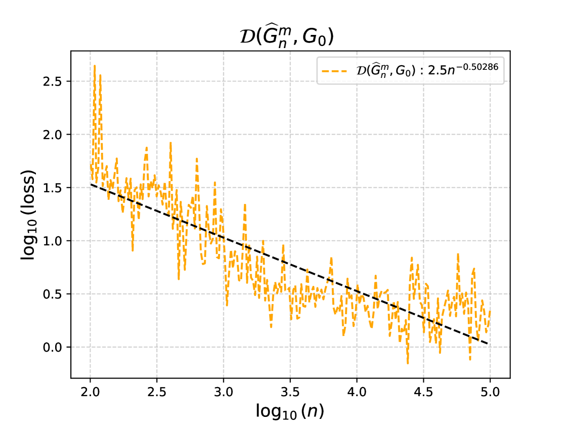
Contributions. We introduce a fast-rate-aware Voronoi distance for SGMoE that augments the unified exact- and over-fit loss with merged-moment couplings inside multi-covered Voronoi cells (eq. 6). This exposes slow directions created by redundant atoms, motivates a hierarchical merge operator, and yields an aggregation path (dendrogram) on mixing measures. Along this path we prove a monotone strengthening of the loss (Lemma 1), obtain near-parametric finite-sample rates for the aggregated estimators together with height and likelihood control (Theorems 1, 2 and 3 and Table 1), and derive a sweep-free dendrogram selection criterion (DSC) that is consistent and avoids multi- training (Theorems 4, 1 and 3). Empirically, DSC is less prone to overfitting than AIC/BIC/ICL under -contamination due to its structural penalty on small heights (Figure 4), and it restores fast parameter rates after aggregation in over-specified SGMoE (Figure 2). To our knowledge this is the first method that couples finite-sample, fast-rate-aware merging with consistent model selection for SGMoE, avoiding multi-size training while preserving statistical efficiency.
| Setting | Loss | ||||
|---|---|---|---|---|---|
| Exact-fit | |||||
| Over-fit | |||||
| Merged |
SGMoE Setting. Let be i.i.d. samples with and . Assume the data are generated by a SGMoE model of order , whose conditional density is
| (1) |
Each expert is Gaussian with mean and variance . We encode parameters via the (not-necessarily normalized) mixing measure
where . Assume is compact and , the support of , is bounded. Assume has a continuous distribution so that the model is identifiable under this convention, a standard mild assumption; see Proposition 1 of Nguyen et al. (2023a).
Maximum Likelihood Over At Most Experts. When the true order is unknown, we estimate within We analyze the exactly specified case , the over-specified case , and the merging scheme using the following maximum likelihood estimator (MLE):
Practical Implication. Practitioners can fit a single over-specified SGMoE with moderate , compute its aggregation path, and select via DSC. This single-fit workflow avoids grid sweeps over , merges near-duplicate atoms to collapse slow directions within Voronoi cells, accelerates parameter convergence, and often recovers the correct expert count even under mild contamination. Dendrogram heights provide a transparent structural summary.
Paper Organization. Section 2 states the unified parameter-rate result and the algebraic exponents . Section 3 introduces the fast-rate-aware distance, merge operator, aggregation path, fast pathwise rates, and DSC. Section 4 illustrates parameter rates, path behaviour, model selection under clean and contaminated regimes, and a real-data application to maize drought-response traits in Section 5. Then, we offer concluding remarks, limitations, and future work in Section 6. Proof sketches appear at the end of Section 3, with full proofs deferred to the appendix. Additional biological background, preprocessing details for the maize dataset, and further geometric and technical discussion are provided in the supplementary material.
Notation. Throughout the paper, for any natural number we abbreviate by . Given two sequences of positive real numbers and , we write (equivalently, ) to mean that there exists a constant such that for all . For a vector , set , and let denote its -norm; by default, refers to the -norm unless otherwise stated. We also use for the Frobenius norm of a matrix . For any set , denotes its cardinality. Finally, for two probability density functions and with respect to the Lebesgue measure , define as their Total Variation distance, while denotes the squared Hellinger distance between them. Let be the parameter space. Write for the collection of discrete probability measures on with exactly atoms, and for those with at most atoms. For a mixing measure , we (slightly abusively) refer to each component as an “atom,” comprising both its weight and parameter . When clear from context, we drop and simply write and .
2 PRELIMINARIES
We present a unified result for the parameter estimation rate of the MLE in the SGMoE that simultaneously covers the exact-specified case () and the over-specified case (), building on Nguyen et al. (2023a).
Voronoi Cells. For a candidate mixing measure and the true , define for :
| (2) |
where we denote . We use the softmax-translation from identifiability (cf. Proposition 1 of Nguyen et al., 2023a) and the shorthand , , , . For notational simplicity, we write instead of .
Algebraic Obstruction and Exponents. For , let be the smallest integer determined by the polynomial system as follows: given the polynomial system
| (3) |
admits no non-trivial solution (all and at least one ). The ranges of in the above sum satisfy . For general dimension and parameter , finding the exact value of is a non-trivial central problem in algebraic geometry (Sturmfels, 2002). Known values:
Fact 1 (Nguyen et al., 2023a, Lemma 1).
For any : , , and for .
Classical Overfit-Aware Voronoi Distance. Define a single loss that reduces to the exact-fit metric when each cell has one atom, and adds over-fit penalties otherwise:
| (4) | |||
When for all (i.e., ), eq. 4 equals the exact-fit metric ; if some (i.e., ), eq. 4 adds the higher-order penalties determined by .
Fact 2 (Nguyen et al., 2023a, Theorems 1 and 2).
There exist universal constants (depending only on and ) s.t. the MLE of order satisfies
| (5) |
Remarks. (i) If (all ), then and eq. 5 yields the exact-specified rate implying parametric ( up to logs) estimation of , (up to translation), , , for all . (ii) If (some ), the same bound holds for , while the exponents inside eq. 4 encode the slower algebraic behavior of over-covered parameters within each Voronoi cell.
3 FAST-RATE-AWARE EXPERT AGGREGATION IN SGMOE
3.1 Why Merge Experts? The Rate Gap
Building on Section 2, identifiability and the unified parameter-rate bound (Fact 2) imply that converting density accuracy into parameter accuracy hinges on a suitable inverse (loss) inequality. When the model is over-specified (), several fitted atoms may fall into the same Voronoi cell (defined in eq. 2), which induces a rate gap: single-covered truths achieve (near) parametric rates, whereas multi-covered truths converge more slowly with exponents governed by from Section 2. To exploit this, we (i) refine the loss to expose mergeable structure, and (ii) aggregate (merge) near-duplicate atoms to recover fast rates and guide model order selection.
3.2 A Fast-Rate-Aware Voronoi Distance
Our Proposal. Let denote the over-fit Voronoi loss from eq. 4 and be as in eq. 2. We augment it with first-order “merged-moment” couplings inside multi-covered cells to obtain
| (6) |
Link to Section 2. The penalties inside eq. 6 are consistent with the exponents that appear in the unified loss eq. 4: when , reduces to the exact-fit metric ; when , the added block-sums control the slow directions and quantify how well the cell behaves as if merged.
Motivation for Merging. Because the slow rates originate from multiple atoms sharing a cell, replacing these atoms by their softmax-weighted aggregate collapses the problematic directions and restores first-order (parametric) behavior for the merged parameters. Thus, both (i) certifies where merging is beneficial (large intra-cell terms) and (ii) predicts the rate improvement obtained by aggregation, which we leverage next for hierarchical merging and model selection.
3.3 A Merge Operator Tailored to SGMoE
Connection to Section 2 and Novelty. The unified rate result in Section 2 shows that parameter convergence hinges on how fitted atoms distribute across Voronoi cells; multi-covered cells induce slower algebraic behavior governed by . The merge operator below is the first ingredient of our contribution: it operationalizes that insight by collapsing near-duplicate atoms within a cell using softmax-weighted updates. This turns slow, multi-component directions into a single, first-order direction, setting up our fast pathwise rates (Theorem 1) and height/likelihood controls (Theorems 2 and 3).
Rate-Weighted Dissimilarity. For with , define
| (7) |
Pick and replace the pair by the softmax-weighted aggregate
| (8) |
Then we define . A description of the whole procedure can be seen in Algorithm 1. The choice of merging atoms and deriving the new atom (eqs. 7 and 8) are in particular faithful to hierarchical clustering and -means algorithms.
3.4 The Hierarchical View of Aggregation Path
Transition and Main Idea. The merge step converts local redundancy into a single effective atom. Repeating it induces a global hierarchy, the aggregation path, along which our new analysis proves a monotone strengthening of the loss and, crucially, fast convergence at every level. This bridges Section 2 (unified loss but slow rates) with a constructive, data-driven path that achieves the same near-parametric behavior after aggregation.
Having presented the algorithm to choose and merge a mixing measure with atoms to atoms, we now describe the dendrogram (hierarchical aggregation) of that emerges by repeatedly applying the merging procedure.
Dendrogram (Hierarchical Aggregation). Iterate the merge in eqs. 7 and 8 from down to , generating . Define the dendrogram with containing levels, the -th level holding the atoms of , storing the links between merged pairs across adjacent levels, and with The quantity is the height between levels and .
When we represent on a graph, is the height between -th level and -th level. The procedure to construct the dendrogram of is given by Algorithm 2.
Monotone Strengthening of the Loss (Bridge to Fast Rates). The following lemma formalizes that each merge step cannot increase our fast-rate-aware distance to , making the path progressively easier to estimate:
Lemma 1.
As , with constants depending only on , , and .
Behavior of the Path for the MLE (Main Fast-Rate Theorem). Leveraging the monotonicity above together with the unified inverse bound from Section 2, we obtain fast rates at every level of the path, including the exact-fit and under-fit levels where aggregation recovers optimal parametric rate behavior:
Theorem 1 (Fast convergence rates along the path).
There exist universal constants such that for all and , we have
| (9) | |||
3.5 Heights and Likelihood Along the Path
Transition from Structure to Statistics. Heights summarize structural redundancy; likelihood captures statistical fit. Our second set of novel guarantees shows (i) heights shrink at a rate dictated by , and (ii) the empirical likelihood concentrates to its population counterpart along the path.
Height Definitions. For all and , let
| (10) |
and let be the analogous height on the true path. Then:
Theorem 2 (Height control).
For all and , and
with constants depending only on , , and .
Likelihood. We define empirical average log-likelihood and population average log-likelihood as follow: and .
Condition K. There exist positive constants and such that for all sufficiently small and such that , we have .
Theorem 3 (Likelihood concentration on the path).
Assume Condition K hold. Then, for any , Moreover, for , in -probability as .
3.6 Choosing the Number of Experts via a Height-Likelihood Rule
Novel Model Selection Principle. By combining structural signal (heights) and statistical fit (likelihood), our DSC favors models that are both well-separated and well-supported by the data, unlike AIC/BIC/ICL, which ignore the geometry of the fitted atoms.
DSC Definition. For each level , define
where the weight satifies . A practical choice is . Select
Theorem 4 (Consistency of model selection).
Assume that data are generated by a softmax-gated Gaussian MoE, the parameter space is compact, the covariate support is bounded, the DSC uses a penalty satisfying as above, and the true component . Then in -probability as .
Interpretation. Unlike pure likelihood criteria (AIC/BIC/ICL), also penalizes structural closeness through . Small heights indicate either redundant atoms (near-duplicates) or atoms with tiny softmax weights; both are symptomatic of over-specification. The joint use of heights and likelihood therefore yields a more robust selection rule in SGMoE.
3.7 Proof Sketches
We sketch the proofs of Lemmas 1, 1, 2, 3 and 4, which together establish monotonicity along the dendrogram path and consistency of the dendrogram-based model selection. We first motivate the fast-rate-aware Voronoi distance in eq. 6. When , over-specification yields Voronoi cells with . Repeatedly merging such atoms eventually makes every cell singleton, which motivates our construction. Using the density decomposition
we analyze the sums over indices with under . For clarity, we also consider with , which corresponds to . This reasoning leads to the merging algorithm.
Proof Sketch of Lemma 1. Proceed by induction on and justify . As , extract a sequence that satisfies and there exist , with and for all . The minimizing pair must belong to a common . Using eq. 8 and Jensen’s inequality for the convex maps and , it suffices to show
which yields the desired monotonicity.
Proof Sketch of Theorem 1. Combine Lemma 1 with an inverse bound for . Following Nguyen et al., 2023a, establish
and use Proposition 2 in Nguyen et al., 2023a,
to derive the rate for . Apply Lemma 1 to obtain the bounds for . For , combine the previous rate with the merging formula to conclude.
Proof Sketch of Theorem 2. Use Theorem 1 and the fact that any merged pair lies in the same Voronoi cell. Inequalities analogous to those in Lemmas 1 and 1 translate parameter rates into height bounds.
Proof Sketch of Theorem 3. Consider three cases. If , invoke empirical process tools (van de Geer, 2000) and comparisons between Hellinger and Wasserstein distances (Chen, 1995; Villani, 2003, 2009). If , combine Theorem 1 with verification that satisfies Condition K. If , conclude via standard convergence arguments.
Finally, Theorem 4 follows from Theorems 2 and 3.
4 SIMULATION STUDIES
We first show that the dendrogram-based merge yields fast convergence of the mixing measure: starting from an over-fitted estimator that converges slowly, the merged estimator approaches the truth quickly. We then assess model selection via DSC against AIC, BIC, and ICL. Unlike these single-shot selectors, the dendrogram offers a hierarchical view of the fitted atoms, clarifying redundancy and structure. All simulations were run in Python 3.12 on a standard Unix-based system.
Numerical Schemes. The ground-truth mixing measure is
For each experiment, varies on a logarithmic grid from to , yielding sizes in . At each , we generate datasets from and compute the exact-fitted MLE and the over-fitted MLE () using an EM variant of Chamroukhi et al. (2009). EM stops at tolerance or 2000 iterations. Because the softmax gate in eq. 1 is translation-invariant, we fix a baseline by setting and .
To stabilize estimation and highlight asymptotics, EM is favorably initialized. For each replication and , split into disjoint sets , each nonempty. For , draw from a Gaussian centered at with small covariance. After estimating , apply the merging procedure in Algorithm 2 to obtain .
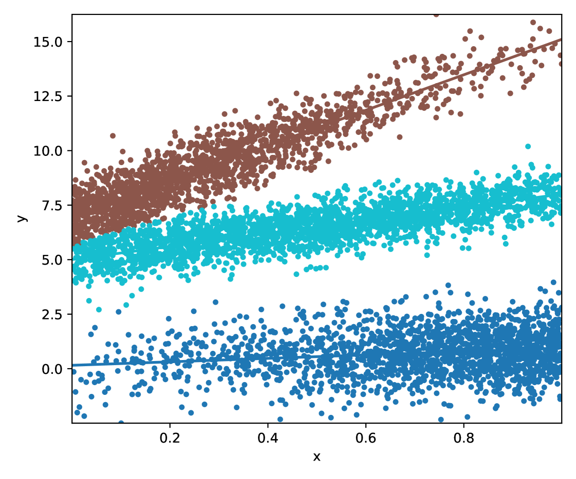
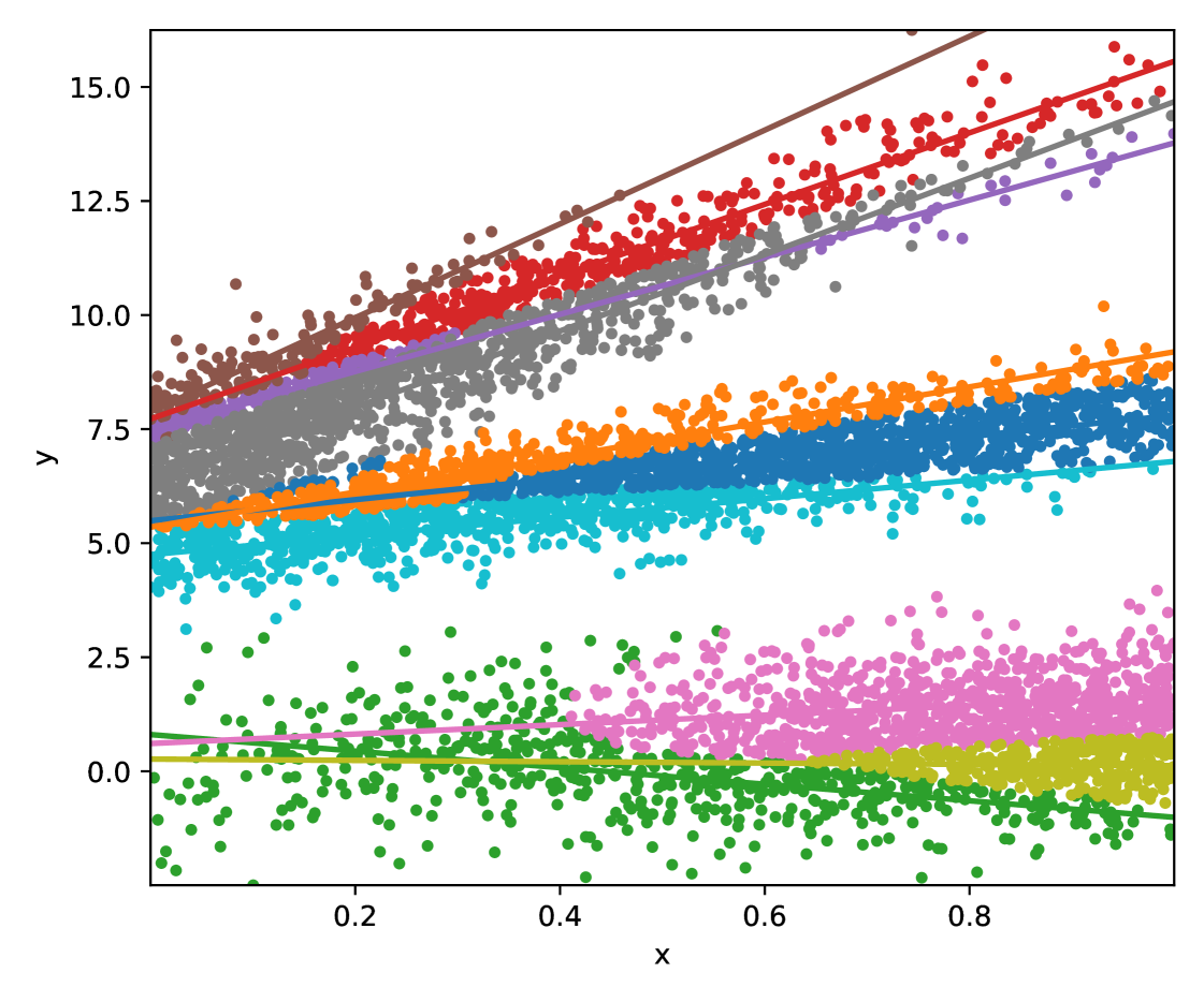
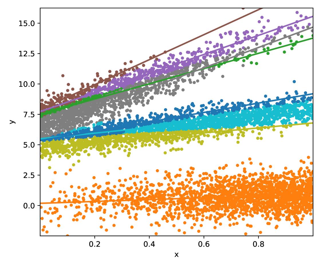
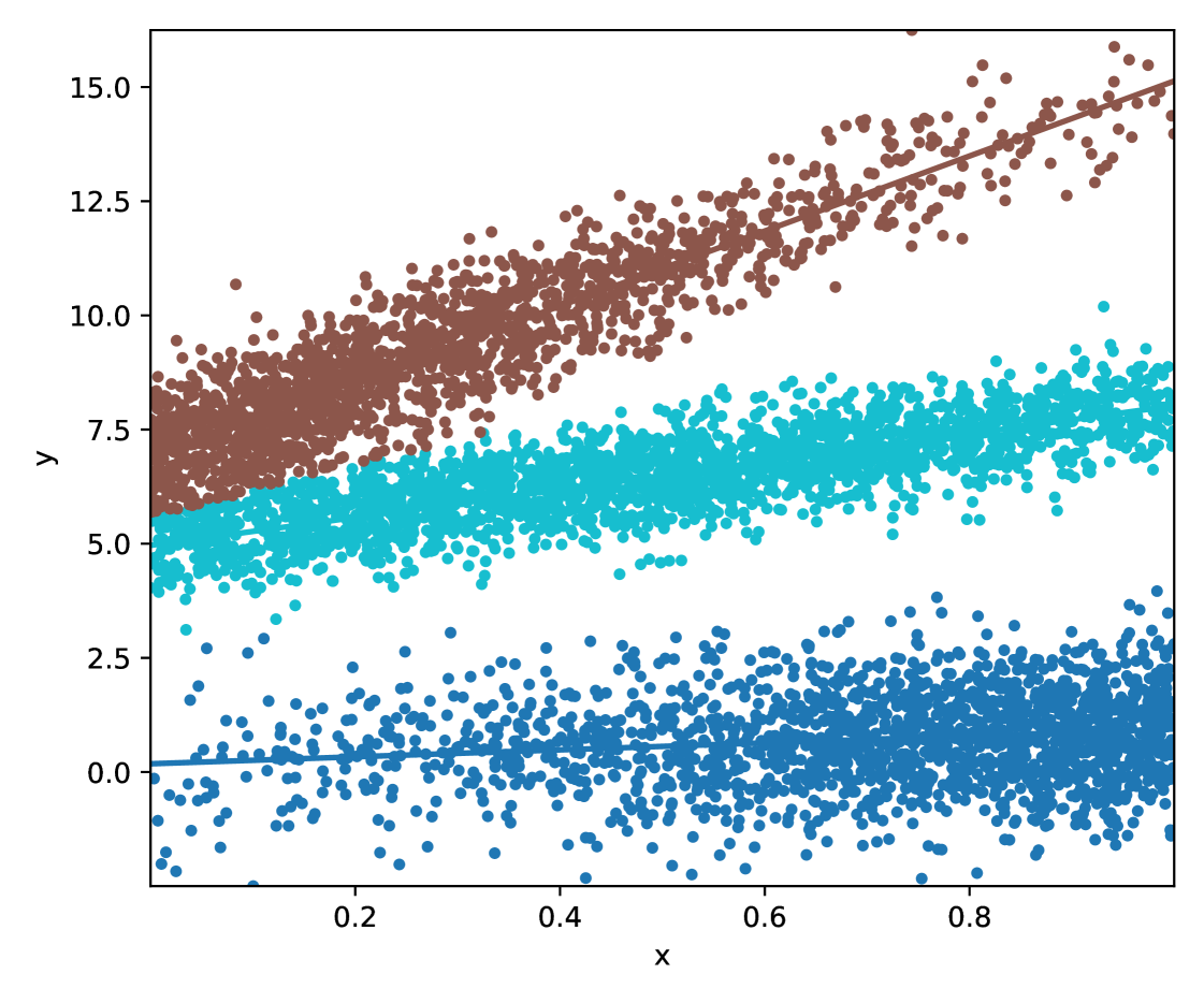
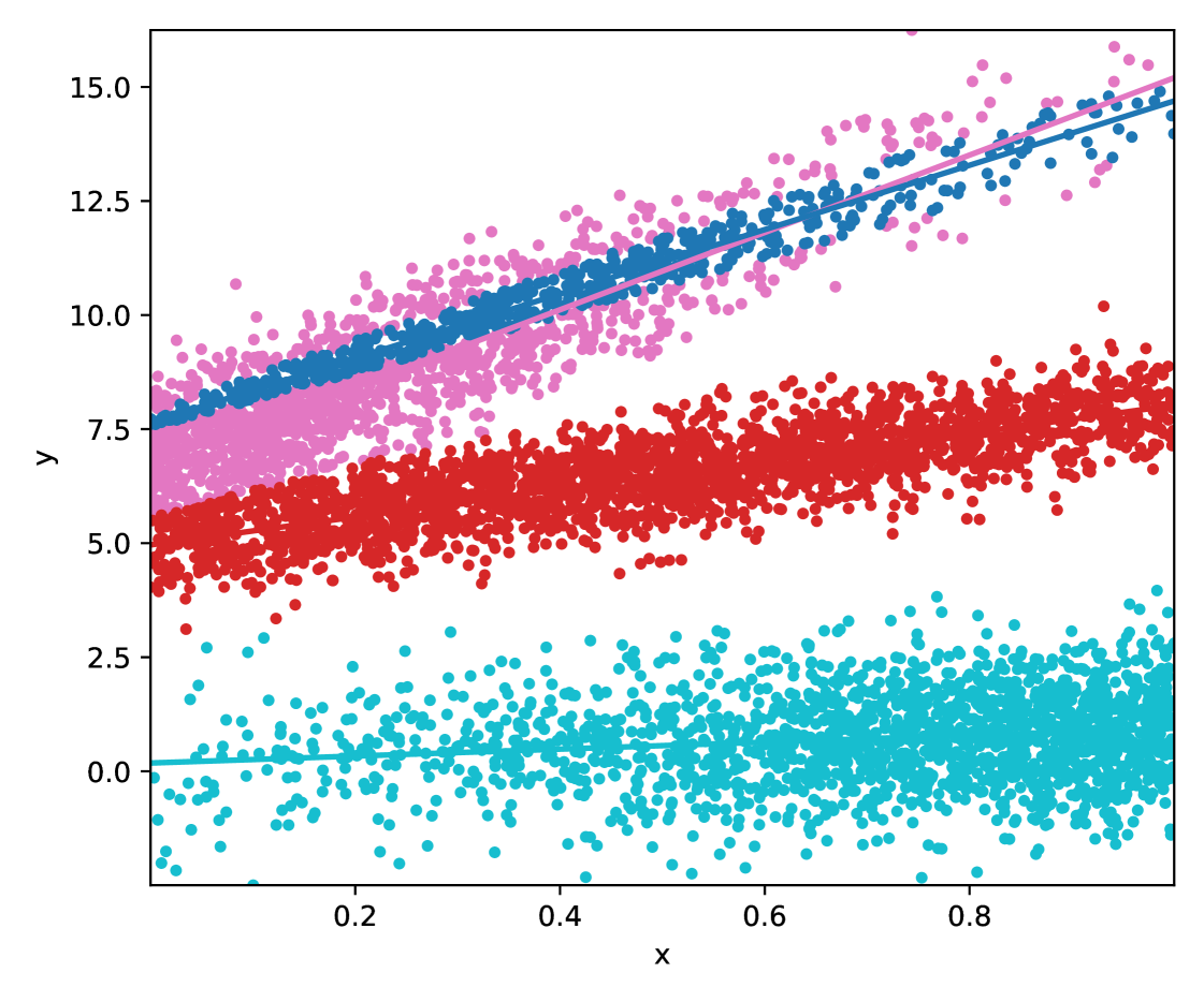
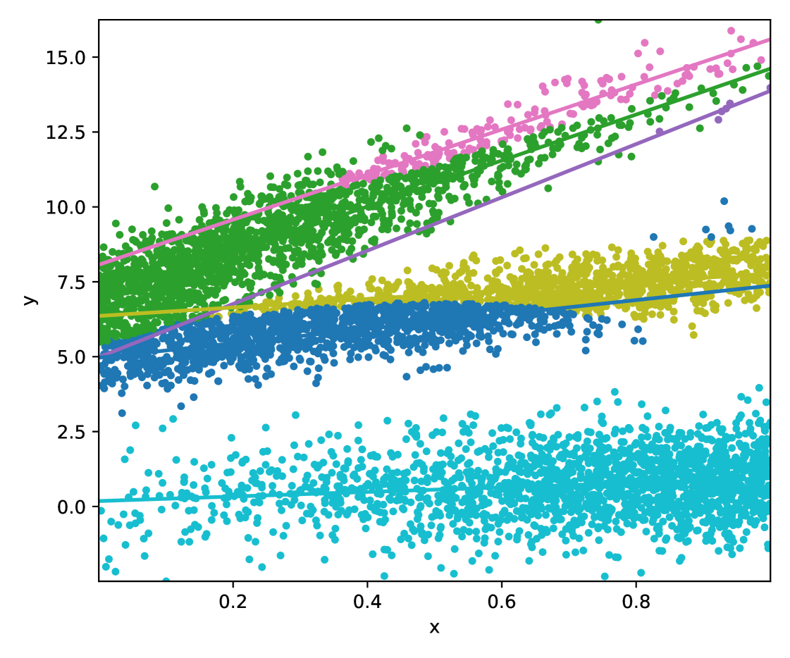
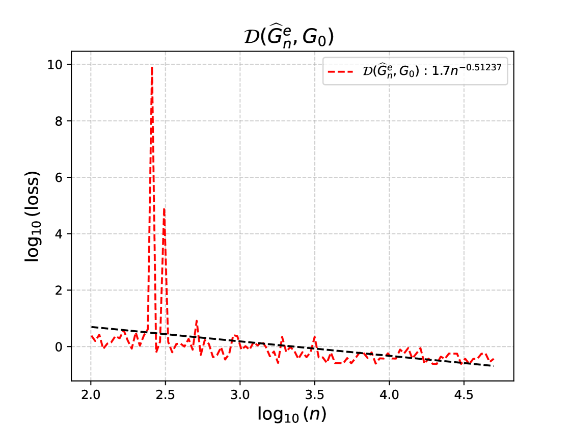
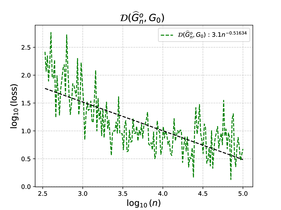
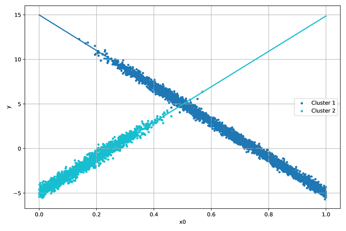
Fast Parameter Estimation via the Dendrogram. We measure accuracy with the Voronoi distance in eq. 6. For the exact-fitted setting, we use replicates over sample sizes with ; for the over-fitted setting, replicates over sizes with ; for the merged estimator, replicates over sizes with . The average loss and a reference slope are shown in Figure 2. Results match Theorem 1: the exact-fitted and merged estimators attain the optimal rate toward , while merging drives the over-fitted estimator to the exact-fit level. For illustration of Algorithm 2, Figure 1 considers as follows:
| (11) |
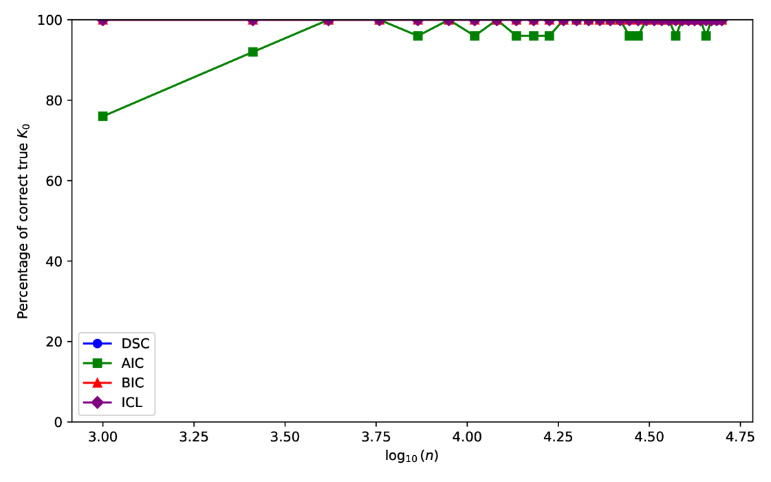
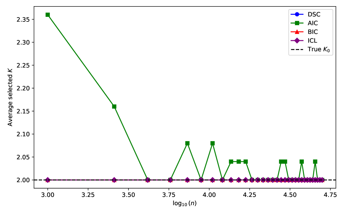
Model Selection with DSC. We compare DSC to AIC, BIC, and ICL over sample sizes with and . For each method, we report the selection frequency of and the average selected size (see Figure 3). AIC/BIC/ICL fit a model for each via EM and pick the best by the corresponding criterion. DSC fits a single SGMoE with , builds its dendrogram, and evaluates the criterion with (Section 3.6). AIC tends to overestimate at small , while all methods recover for large .
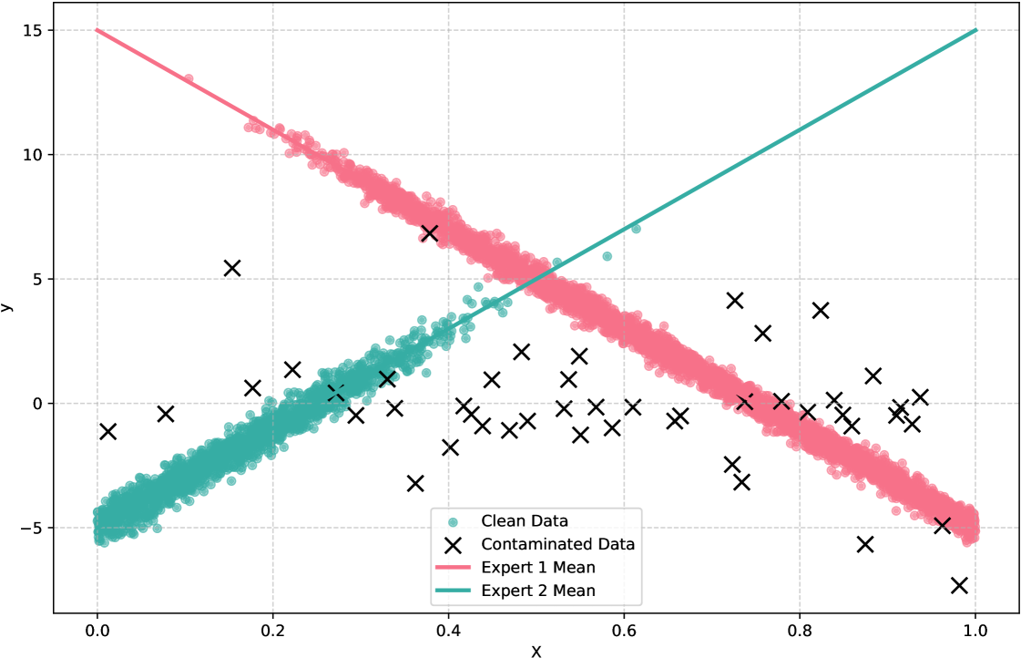
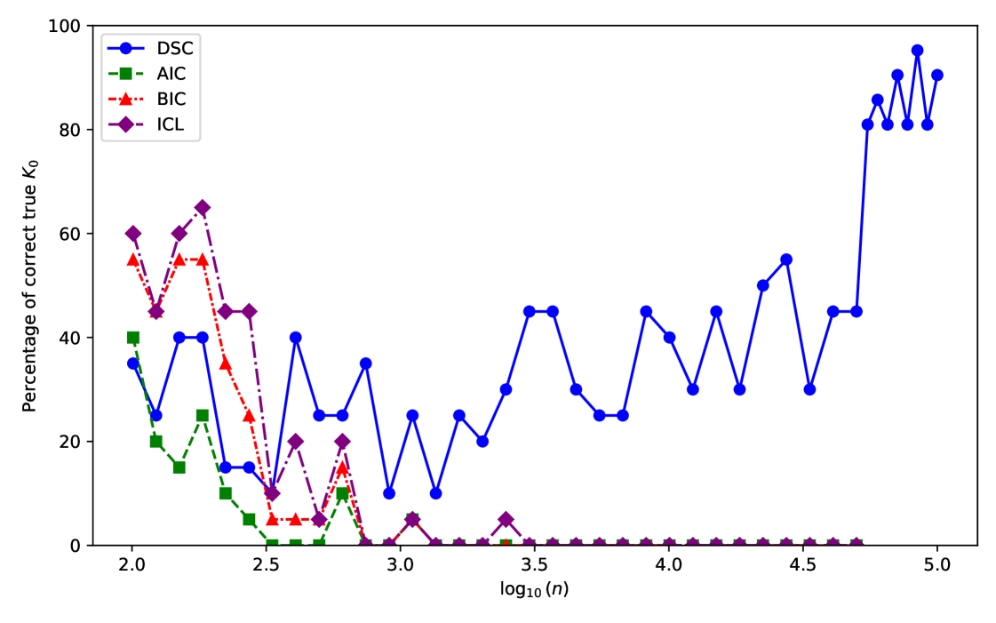
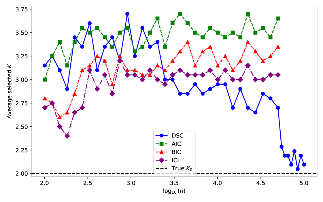
Misspecified Regime. We study -contamination with , where is Laplace. Figure 4(a) shows the contaminated sample (). Figures 4(b) and 4(c) report the proportion of correct selections and the average selected size. AIC/BIC/ICL behave similarly: they may find at small , but tend to overselect as grows, indicating sensitivity to contamination. DSC, leveraging dendrogram structure, is more robust and continues to select with non-negligible frequency even at large .
5 REAL DATA APPLICATION
We illustrate the dendrogram of mixing measures obtained from our SGMoE model using a real dataset from the study in Blein-Nicolas et al. (2024). The data originate from a large-scale experiment on maize aimed at understanding the genetic and molecular bases of drought-responsive traits from proteins expressed in the leaf (Prado et al., 2018; Blein-Nicolas et al., 2020), where 254 genotypes representing the genetic diversity of dent maize were grown under two watering conditions and phenotyped for seven ecophysiological traits.
After preprocessing and removing missing data as described in Blein-Nicolas et al. (2024), the final dataset consists of 233 maize genotypes (), two ecophysiological traits (outputs), which are water use (WU) and the proteins quantified under the water deficit (WD) condition, and 973 protein variables (inputs, ). To reduce dimensionality and remove irrelevant features, we apply a Lasso procedure to select protein variables most associated with the target trait and primarily focus on the ecophysiological trait WU.
We then fit the SGMoE model with clusters. To ensure a more robust initialization, we first cluster the data into 20 groups using the K-Means algorithm. The resulting cluster assignments are then used to initialize the gating and expert parameters of the SGMoE model, providing a stable starting point for the subsequent steps of the EM algorithm.
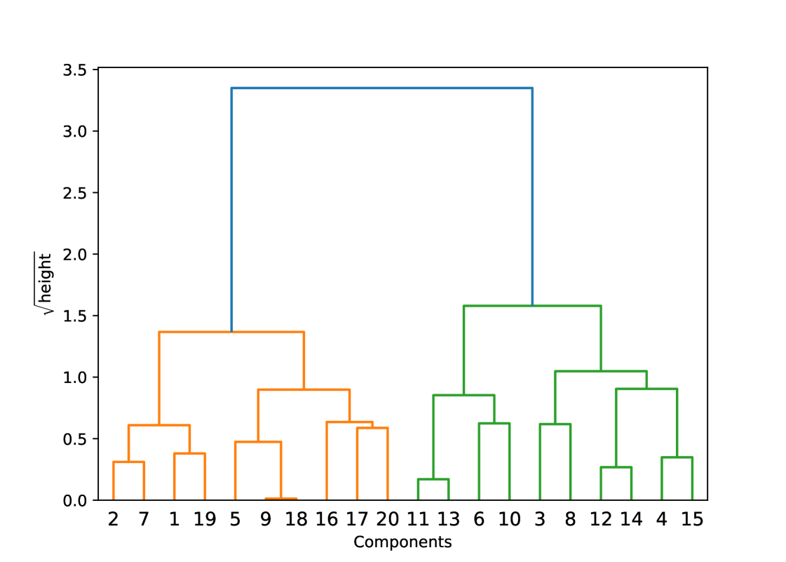
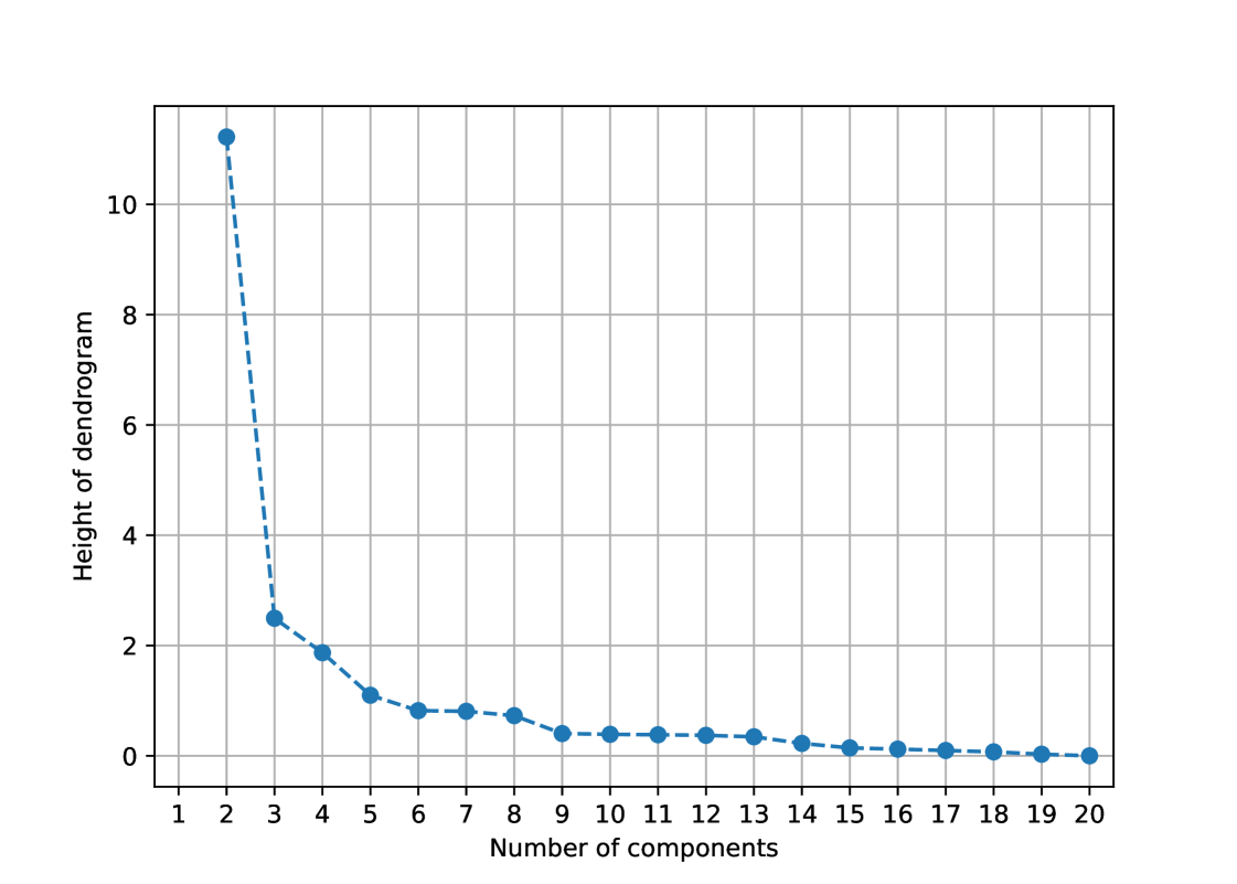
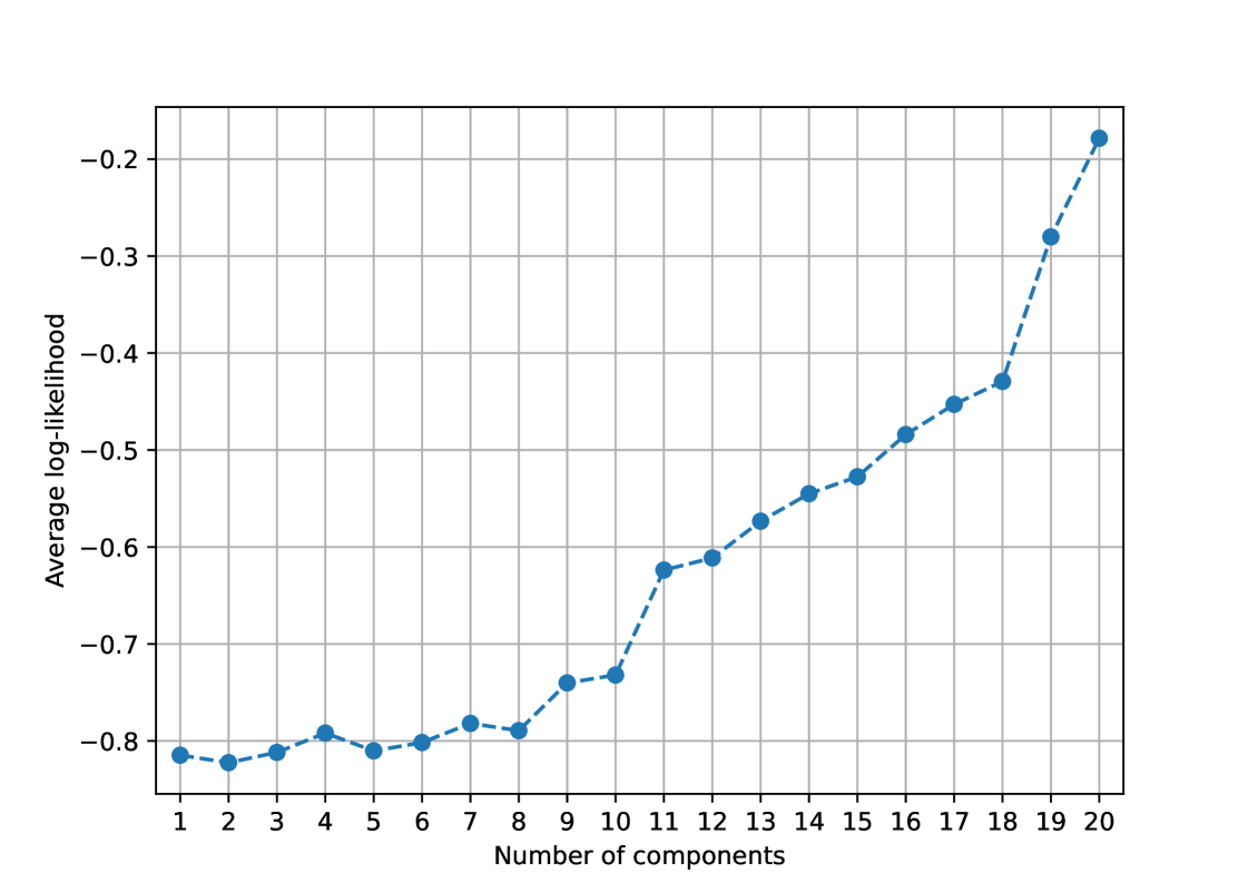
Figure 5(a) displays the dendrogram of the fitted mixing measure obtained by Algorithm 2, which reveals the hierarchical structure underlying the data. In this experiment, both BIC and ICL select a single component, while DSC selects 2 components, and AIC overestimates with 18 components. The corresponding heights and average log-likelihoods across levels are shown in Figure 5(b) and Figure 5(c), respectively. We observe that the merging heights generally decrease and approach zero, while the average log-likelihood stabilizes in a few initial levels. Notably, the height at level 2 is much larger than those at subsequent levels, suggesting that there should be two clusters in the data.
The dendrogram not only facilitates effective model selection but also unveils the hierarchical relationships among mixture components, thereby enhancing the interpretability of the estimated parameters in complex biological data settings.
6 CONCLUSION
This work shows that rate-aware geometry, realized through a Voronoi distance together with merging and dendrograms of mixing measures, delivers both fast parameter estimation and consistent, sweep-free model selection in SGMoE. We hope these ideas spur further advances in structured mixture models and expert architectures. Our analysis assumes linear softmax gates, Gaussian experts, compact , and bounded covariate support. Extending the theory beyond these settings will require additional regularity and tail controls. Exact values of are known for ; for only lower bounds are available. While our guarantees use these bounds, sharper algebraic results would further tighten rates.
Acknowledgments
This project was funded primarily by the Australian Research Council Centre of Excellence for the Mathematical Analysis of Cellular Systems (CE230100001), which supported TrungTin Nguyen and Christopher Drovandi. Christopher Drovandi was also supported by an Australian Research Council Future Fellowship (FT210100260). Additional support was provided by Vietnam National University Ho Chi Minh City (VNU-HCM) under grant number A2025-18-02. The authors also acknowledge Dr. Dat Do (University of Chicago) for helpful discussions about the dendrogram of mixing measures for mixture models (Do et al., 2024).
References
- A new look at the statistical model identification. IEEE Transactions on Automatic Control 19 (6), pp. 716–723. External Links: Document Cited by: §1. ↩ 1
- A method of moments for mixture models and hidden markov models. In COLT, Cited by: §1. ↩ 1
- Statistical guarantees for the EM algorithm: from population to sample-based analysis. Annals of Statistics 45, pp. 77–120. Cited by: §1. ↩ 1
- VLMo: unified vision-language pre-training with mixture-of-modality-experts. In Advances in Neural Information Processing Systems, Cited by: §1. ↩ 1
- Identifying Brexit voting patterns in the British house of commons: an analysis based on Bayesian mixture models with flexible concomitant covariate effects. Journal of the Royal Statistical Society Series C: Applied Statistics 73 (3), pp. 621–638. External Links: ISSN 0035-9254, Link, Document Cited by: §1. ↩ 1
- Assessing a mixture model for clustering with the integrated completed likelihood. IEEE Transactions on Pattern Analysis and Machine Intelligence 22 (7), pp. 719–725. External Links: Document Cited by: §1. ↩ 1
- Nonlinear network-based quantitative trait prediction from biological data. Journal of the Royal Statistical Society Series C: Applied Statistics 73 (3), pp. 796–815. External Links: ISSN 0035-9254, Document, Link, https://academic.oup.com/jrsssc/article-pdf/73/3/796/58185677/qlae012.pdf Cited by: Appendix A, Appendix A, Appendix A, §5, §5. ↩ 5 A
- A systems genetics approach reveals environment-dependent associations between snps, protein coexpression, and drought-related traits in maize. Genome Research 30 (11), pp. 1593–1604. Cited by: Appendix A, §5. ↩ 5 A
- Time series modeling by a regression approach based on a latent process. Neural Networks 22 (5–6), pp. 593–602. External Links: ISSN 0893-6080, Link, Document Cited by: §4. ↩ 4
- Optimal Rate of Convergence for Finite Mixture Models. The Annals of Statistics 23 (1), pp. 221 – 233. Note: Publisher: Institute of Mathematical Statistics External Links: Link, Document Cited by: §1, §3.7. ↩ 1 3.7
- Towards Understanding the Mixture-of-Experts Layer in Deep Learning. In Advances in Neural Information Processing Systems, A. H. Oh, A. Agarwal, D. Belgrave, and K. Cho (Eds.), External Links: Link Cited by: §1. ↩ 1
- Risk Bounds for Mixture Density Estimation on Compact Domains via the h-Lifted Kullback–Leibler Divergence. Transactions on Machine Learning Research. Note: Accept with minor revision External Links: Link Cited by: §1. ↩ 1
- DeepSeekMoE: towards ultimate expert specialization in mixture-of-experts language models. In Proceedings of the 62nd Annual Meeting of the Association for Computational Linguistics (Volume 1: Long Papers), L. Ku, A. Martins, and V. Srikumar (Eds.), Bangkok, Thailand, pp. 1280–1297. External Links: Link, Document Cited by: Appendix B. ↩ B
- Dendrogram of mixing measures: Learning latent hierarchy and model selection for finite mixture models. arXiv preprint arXiv:2403.01684. Cited by: Appendix B, §1, §6. ↩ 1 6 B
- Strong identifiability and parameter learning in regression with heterogeneous response. Electronic Journal of Statistics 19 (1), pp. 131 – 203. Note: Publisher: Institute of Mathematical Statistics and Bernoulli Society External Links: Link, Document Cited by: §1. ↩ 1
- HyperRouter: Towards Efficient Training and Inference of Sparse Mixture of Experts. In Proceedings of the 2023 Conference on Empirical Methods in Natural Language Processing, Singapore. Cited by: Appendix B, §1. ↩ 1 B
- An image is worth 16x16 words: transformers for image recognition at scale. In International Conference on Learning Representations, External Links: Link Cited by: §1. ↩ 1
- Optimal estimation of high-dimensional Gaussian location mixtures. The Annals of Statistics 51 (1), pp. 62 – 95. Note: Publisher: Institute of Mathematical Statistics External Links: Link, Document Cited by: §1. ↩ 1
- Sharp analysis of expectation-maximization for weakly identifiable models. AISTATS. Cited by: §1. ↩ 1
- Singularity, misspecification, and the convergence rate of EM. Annals of Statistics 44, pp. 2726–2755. Cited by: §1. ↩ 1
- Learning factored representations in a deep mixture of experts. In ICLR Workshops, Cited by: §1. ↩ 1
- Switch transformers: scaling to trillion parameter models with simple and efficient sparsity. Journal of Machine Learning Research 23, pp. 1–39. Cited by: Appendix B, §1. ↩ 1 B
- Mixture of expert posterior surrogates for approximate Bayesian computation. In JDS 2022 - 53èmes Journées de Statistique de la Société Française de Statistique (SFdS), Lyon, France. Cited by: §1. ↩ 1
- Summary statistics and discrepancy measures for approximate Bayesian computation via surrogate posteriors. Statistics and Computing 32 (5), pp. 85. External Links: ISSN 1573-1375, Link, Document Cited by: §1. ↩ 1
- Extended Bayesian Information Criteria for Gaussian Graphical Models. In Advances in Neural Information Processing Systems, J. Lafferty, C. Williams, J. Shawe-Taylor, R. Zemel, and A. Culotta (Eds.), Vol. 23. External Links: Link Cited by: §1. ↩ 1
- Labor market entry and earnings dynamics: Bayesian inference using mixtures-of-experts Markov chain clustering. Journal of Applied Econometrics 27 (7), pp. 1116–1137. External Links: Link, Document Cited by: §1. ↩ 1
- Analysing plant closure effects using time-varying mixture-of-experts Markov chain clustering. The Annals of Applied Statistics 12 (3), pp. 1796 – 1830. Note: Publisher: Institute of Mathematical Statistics External Links: Link, Document Cited by: §1. ↩ 1
- Keeping the balance—Bridge sampling for marginal likelihood estimation in finite mixture, mixture of experts and Markov mixture models. Brazilian Journal of Probability and Statistics 33 (4), pp. 706 – 733. External Links: Link, Document Cited by: §1. ↩ 1
- Rates of convergence for the Gaussian mixture sieve. The Annals of Statistics 28 (4), pp. 1105 – 1127. External Links: Link, Document Cited by: §1. ↩ 1
- On posterior contraction of parameters and interpretability in Bayesian mixture modeling. Bernoulli 27 (4), pp. 2159 – 2188. External Links: Link, Document Cited by: §1. ↩ 1
- Tight bounds for learning a mixture of two gaussians. In STOC, Cited by: §1. ↩ 1
- Strong identifiability and optimal minimax rates for finite mixture estimation. The Annals of Statistics 46 (6), pp. 2844–2870. Cited by: §1. ↩ 1
- A Unified Framework for Variable Selection in Model-Based Clustering with Missing Not at Random. In The Thirty-ninth Annual Conference on Neural Information Processing Systems, External Links: Link Cited by: §1. ↩ 1
- Convergence rates of parameter estimation for some weakly identifiable finite mixtures. The Annals of Statistics 44 (6), pp. 2726 – 2755. External Links: Link, Document Cited by: §F.4, §1, §1, Fact 7. ↩ 1 F.4
- On strong identifiability and convergence rates of parameter estimation in finite mixtures. Electronic Journal of Statistics 10 (1), pp. 271–307. Cited by: §1. ↩ 1
- Convergence Rates for Gaussian Mixtures of Experts. Journal of Machine Learning Research 23 (323), pp. 1–81. External Links: Link Cited by: §1, §1. ↩ 1
- Adaptive mixtures of local experts. Neural computation 3 (1), pp. 79–87. Cited by: §1. ↩ 1
- On the identifiability of mixtures-of-experts. Neural Networks 12 (9), pp. 1253–1258. External Links: ISSN 0893-6080, Link, Document Cited by: §F.2. ↩ F.2
- Hierarchical mixtures of experts and the EM algorithm. Neural computation 6 (2), pp. 181–214. Cited by: §1. ↩ 1
- Estimation and group-feature selection in sparse mixture-of-experts with diverging number of parameters. Journal of Statistical Planning and Inference, pp. 106250. External Links: ISSN 0378-3758, Link, Document Cited by: §1. ↩ 1
- M3ViT: Mixture-of-Experts Vision Transformer for Efficient Multi-task Learning with Model-Accelerator Co-design. In NeurIPS, Cited by: §1. ↩ 1
- Uniform convergence rates for maximum likelihood estimation under two-component gaussian mixture models. arXiv preprint arXiv:2006.00704. Cited by: §1. ↩ 1
- Mixture of Gaussian regressions model with logistic weights, a penalized maximum likelihood approach. Electronic Journal of Statistics 8 (1), pp. 1661–1695. Cited by: §1. ↩ 1
- Joint learning of Gaussian graphical models in heterogeneous dependencies of high-dimensional transcriptomic data. In The 16th Asian Conference on Machine Learning (Conference Track), External Links: Link Cited by: §1. ↩ 1
- Approximation results regarding the multiple-output Gaussian gated mixture of linear experts model. Neurocomputing 366, pp. 208–214. External Links: ISSN 0925-2312, Link, Document Cited by: §1. ↩ 1
- Practical and theoretical aspects of mixture-of-experts modeling: An overview. Wiley Interdisciplinary Reviews: Data Mining and Knowledge Discovery 8 (4), pp. e1246. Cited by: §1. ↩ 1
- A universal approximation theorem for mixture-of-experts models. Neural computation 28 (12), pp. 2585–2593. Cited by: §1. ↩ 1
- On the large-sample limits of some Bayesian model evaluation statistics. arXiv preprint arXiv:2502.03846. Cited by: §1. ↩ 1
- Approximations of conditional probability density functions in Lebesgue spaces via mixture of experts models. Journal of Statistical Distributions and Applications 8 (1), pp. 13. External Links: ISSN 2195-5832, Link, Document Cited by: §1. ↩ 1
- Approximation rates for finite mixtures of location-scale models. arXiv preprint arXiv:2508.10612. Cited by: §1. ↩ 1
- Modifications of the BIC for order selection in finite mixture models. 2506.20124. External Links: Link Cited by: §1. ↩ 1
- A General Theory for Softmax Gating Multinomial Logistic Mixture of Experts. In Proceedings of The 41st International Conference on Machine Learning, Cited by: §1. ↩ 1
- Statistical perspective of top-k sparse softmax gating mixture of experts. External Links: 2309.13850, Link Cited by: Appendix B. ↩ B
- Demystifying Softmax Gating Function in Gaussian Mixture of Experts. In Advances in Neural Information Processing Systems, A. Oh, T. Naumann, A. Globerson, K. Saenko, M. Hardt, and S. Levine (Eds.), Vol. 36, pp. 4624–4652. Cited by: Appendix B, Appendix C, Appendix D, §E.2, §E.2, §F.2, §F.2, §F.4, §1, §1, §1, §2, §2, §3.7, §3.7, Fact 1, Fact 2, Fact 3, Fact 4, Fact 5. ↩ 1 2 3.7 B C D E.2 F.2 F.4
- Towards Convergence Rates for Parameter Estimation in Gaussian-gated Mixture of Experts. In Proceedings of The 27th International Conference on Artificial Intelligence and Statistics, S. Dasgupta, S. Mandt, and Y. Li (Eds.), Proceedings of Machine Learning Research, Vol. 238, pp. 2683–2691. External Links: Link Cited by: §1. ↩ 1
- Approximation of probability density functions via location-scale finite mixtures in Lebesgue spaces. Communications in Statistics - Theory and Methods 52 (14), pp. 5048–5059. External Links: Link, Document Cited by: §1. ↩ 1
- Non-asymptotic model selection in block-diagonal mixture of polynomial experts models. Preprint. arXiv:2104.08959. External Links: Link Cited by: §1. ↩ 1
- Model selection by penalization in mixture of experts models with a non-asymptotic approach. In JDS 2022 - 53èmes Journées de Statistique de la Société Française de Statistique (SFdS), Lyon, France. Cited by: §1. ↩ 1
- Bayesian nonparametric mixture of experts for inverse problems. Journal of Nonparametric Statistics, pp. 1–60. Note: doi: 10.1080/10485252.2024.2426091 External Links: ISSN 1048-5252, Link, Document Cited by: §1. ↩ 1
- A non-asymptotic theory for model selection in high-dimensional mixture of experts via joint rank and variable selection. In AJCAI Australasian Joint Conference on Artificial Intelligence 2023, External Links: Link Cited by: §1. ↩ 1
- Non-asymptotic oracle inequalities for the Lasso in high-dimensional mixture of experts. arXiv:2009.10622. External Links: Link Cited by: §1. ↩ 1
- A non-asymptotic approach for model selection via penalization in high-dimensional mixture of experts models. Electronic Journal of Statistics 16 (2), pp. 4742 – 4822. External Links: Link, Document Cited by: §1. ↩ 1
- Approximation by finite mixtures of continuous density functions that vanish at infinity. Cogent Mathematics & Statistics 7 (1), pp. 1750861. External Links: ISSN null, Link, Document Cited by: §1. ↩ 1
- Model Selection and Approximation in High-dimensional Mixtures of Experts Models: from Theory to Practice. PhD Thesis, Normandie Université, (en). External Links: Link Cited by: §1. ↩ 1
- Convergence of latent mixing measures in finite and infinite mixture models. The Annals of Statistics 41 (1), pp. 370–400. External Links: Link, Document Cited by: §1, §1. ↩ 1
- Approximation of conditional densities by smooth mixtures of regressions. The Annals of Statistics 38 (3), pp. 1733 – 1766. External Links: Link, Document Cited by: §1. ↩ 1
- Bayesian Inference in Mixtures-of-Experts and Hierarchical Mixtures-of-Experts Models With an Application to Speech Recognition. Journal of the American Statistical Association 91 (435), pp. 953–960. External Links: ISSN 01621459 Cited by: §1. ↩ 1
- CompeteSMoE–Effective Training of Sparse Mixture of Experts via Competition. arXiv preprint arXiv:2402.02526. Cited by: Appendix B, §1. ↩ 1 B
- Phenomics allows identification of genomic regions affecting maize stomatal conductance with conditional effects of water deficit and evaporative demand. Plant, Cell & Environment 41 (2), pp. 314–326. Cited by: Appendix A, §5. ↩ 5 A
- Risk bounds for mixture density estimation. ESAIM: PS 9, pp. 220–229. External Links: Link, Document Cited by: §1. ↩ 1
- Estimating the dimension of a model. The Annals of Statistics 6 (2), pp. 461–464. Cited by: §1. ↩ 1
- Adaptive Bayesian multivariate density estimation with Dirichlet mixtures. Biometrika 100 (3), pp. 623–640. Cited by: §1. ↩ 1
- Information criteria for selecting possibly misspecified parametric models. Journal of Econometrics 71 (1), pp. 207–225. External Links: ISSN 0304-4076, Link, Document Cited by: §1. ↩ 1
- Solving systems of polynomial equations. CBMS Regional Conference Series in Mathematics, American Mathematical Soc.. Cited by: §2. ↩ 2
- Model Selection for Gaussian-gated Gaussian Mixture of Experts Using Dendrograms of Mixing Measures. arXiv preprint arXiv:2505.13052. Cited by: Appendix B, Appendix B, §1. ↩ 1 B
- Fast Model Selection and Stable Optimization for Softmax-Gated Multinomial-Logistic Mixture of Experts Models. Note: _eprint: 2602.07997 External Links: Link Cited by: §1. ↩ 1
- Revisiting Incremental Stochastic Majorization-Minimization Algorithms with Applications to Mixture of Experts. arXiv preprint arXiv:2601.19811. Cited by: §1. ↩ 1
- Empirical Processes in M-estimation. Vol. 6, Cambridge university press. Cited by: §E.4, §3.7, Fact 6. ↩ 3.7 E.4 F.4
- Topics in optimal transportation. Graduate Studies in Mathematics, Vol. 58, American Mathematical Society. External Links: ISBN 0-8218-3312-X Cited by: §3.7. ↩ 3.7
- Optimal transport: old and new. Vol. 338, Springer. Cited by: §3.7. ↩ 3.7
- On the Asymptotic Distribution of the Minimum Empirical Risk. In Forty-first International Conference on Machine Learning, External Links: Link Cited by: §1. ↩ 1
- Randomly initialized EM algorithm for two-component Gaussian mixture achieves near optimality in iterations. Mathematical Statistics and Learning 4, pp. 143–220. Cited by: §1. ↩ 1
- Optimal estimation of Gaussian mixtures via denoised method of moments. The Annals of Statistics 48, pp. 1987–2007. Cited by: §1. ↩ 1
- SpeechMoE: scaling to large acoustic models with dynamic routing mixture of experts. In Interspeech, Cited by: §1. ↩ 1
- Speechmoe2: mixture-of-experts model with improved routing. In ICASSP 2022 - 2022 IEEE International Conference on Acoustics, Speech and Signal Processing (ICASSP), pp. 7217–7221. External Links: Document Cited by: §1. ↩ 1
- Twenty Years of Mixture of Experts. IEEE Transactions on Neural Networks and Learning Systems 23 (8), pp. 1177–1193. External Links: ISSN 2162-2388 VO - 23, Document Cited by: §1. ↩ 1
- Bayesian shrinkage in mixture-of-experts models: identifying robust determinants of class membership. Advances in Data Analysis and Classification 13 (4), pp. 1019–1051. External Links: ISSN 1862-5355, Link, Document Cited by: §1. ↩ 1
Appendix A ADDITIONAL DETAILS ON THE MAIZE DROUGHT-RESPONSE DATA
This appendix provides additional biological context and a more explicit description of the data-processing pipeline used for the real-data illustration in the main paper. The goal is to clarify the provenance of the dataset, the meaning of the response and predictor variables, and the rationale for the preprocessing choices, while avoiding repetition of the main-text discussion.
Biological motivation and data provenance.
The dataset comes from a broader systems-genetics effort on dent maize aimed at linking molecular variation in the leaf proteome to drought-related ecophysiological traits. In that line of work, a genetically diverse maize panel was grown under contrasting watering conditions and characterised using both high-throughput phenotyping and proteomics, with the broader objective of understanding how genotype-dependent molecular responses are related to drought adaptation and plant water-use behaviour (Prado et al., 2018; Blein-Nicolas et al., 2020). The statistical prediction study of Blein-Nicolas et al. (2024) used these biological measurements as a benchmark for multivariate trait prediction from high-dimensional proteomic covariates, specifically considering drought-related traits measured on a panel of 233 maize genotypes with 973 protein predictors (Blein-Nicolas et al., 2024). Systems-genetics reports associated with the same experimental programme also emphasise that the maize data were designed to study drought-related traits by integrating proteomic and genomic information (Blein-Nicolas et al., 2020).
Why this dataset is relevant here.
This dataset is well suited to our SGMoE framework for three reasons. First, the sample is biologically heterogeneous: the maize panel spans substantial genetic diversity, so one should not expect all genotypes to follow a single homogeneous regression relationship. Second, drought response is known to be multi-mechanistic, with different molecular programmes potentially associated with different water-use strategies or stress-response profiles. Third, the predictor space is high-dimensional relative to the sample size, which makes model structure and interpretability especially important. These features make the dataset a natural test bed for a method that combines flexible conditional modelling with hierarchical aggregation and model selection. The resulting fitted components can then be interpreted as latent subgroups of genotypes sharing similar proteomic-to-phenotypic relationships rather than as merely algorithmic clusters.
Raw variables used in the illustration.
Following Blein-Nicolas et al. (2024), we work with a cleaned subset of the original experiment after removing observations with missing values. The final analysis set contains maize genotypes. The biological study recorded two drought-related ecophysiological outputs together with quantitative protein abundances measured under water-deficit conditions, yielding a predictor matrix with 973 protein variables before dimension reduction. In the present illustration, we focus primarily on the ecophysiological trait water use (WU), while the predictors are the leaf protein abundances measured under the water-deficit regime. This choice is scientifically meaningful because WU is directly linked to drought adaptation and integrates the cumulative effect of genotype-specific physiological regulation under stress.
Preprocessing strategy.
The preprocessing follows the protocol used for the statistical benchmark in Blein-Nicolas et al. (2024), with the same starting point of a cleaned matrix after exclusion of incomplete observations. Since the original proteomic representation is very high-dimensional compared with the number of genotypes, we apply a supervised screening step before fitting the SGMoE. Concretely, we use a Lasso-based variable-selection procedure to extract a smaller subset of proteins that are most strongly associated with the target trait, and we retain proteins for the analysis shown in the main paper. This reduction serves two purposes. Statistically, it improves stability in the small-, large- regime and reduces the risk that the fitted experts are driven by noise dimensions. Biologically, it yields a more interpretable model by restricting attention to a compact set of drought-informative protein signals. We stress that this Lasso step is used only as a preprocessing device; the clustering, aggregation path, and model selection are all performed by the SGMoE methodology thereafter.
Model fitting for the SGMoE path.
After preprocessing, we fit an over-specified SGMoE with initial components. Because mixture models can be sensitive to starting values, we initialise the fit using a preliminary -means partition of the genotypes. These initial groups are then used to seed the gating and expert parameters before running the estimation procedure. The purpose of this intentionally over-specified fit is not to interpret all 20 initial components literally, but rather to create a rich starting representation from which the dendrogram path can merge redundant atoms and reveal a more stable low-dimensional structure. In this sense, the over-specified fit plays the same exploratory role as in the synthetic studies: it allows the subsequent aggregation path to separate persistent large-scale structure from small within-cell duplications.
Interpretation of the fitted path.
In the main-text illustration, the fitted dendrogram suggests a pronounced split at level , while the average log-likelihood stabilises quickly along the path. From a biological viewpoint, this pattern is consistent with the idea that the maize panel contains a small number of broad genotype groups with distinct proteomic-response profiles under drought, rather than many sharply separated subpopulations. Thus, the selected two-expert solution should be read as a parsimonious summary of two dominant genotype–phenotype response regimes. The value of the dendrogram is therefore twofold: it provides a data-driven model-selection tool, and it offers a hierarchical view of how more complex over-specified representations collapse into a small number of biologically interpretable regimes.
Why the real-data example is informative for our methodology.
Unlike the synthetic experiments, this dataset does not come with a known ground-truth number of experts. Its role is instead to illustrate the practical behaviour of the pathwise procedure on a genuinely heterogeneous biological problem. In particular, it shows that the dendrogram can remain informative even when standard information criteria disagree strongly, and that the selected solution can still be interpreted in domain terms through genotype–phenotype structure and early likelihood stabilisation. This complements the theory by demonstrating that the SGMoE aggregation path is not only a technical device for proving rates, but also a practically useful summary of heterogeneity in complex omics-assisted prediction problems.
Appendix B OVERVIEW OF MIXTURE AND MOE GEOMETRY
This section provides a unified overview of unconditional mixtures, MoE, and SGMoE, clarifying the geometric and statistical differences that motivate our dendrogram framework.
First, we recall the definitions of unconditional mixtures, MoE, and covariate-free gates.
-
•
Unconditional mixture:
-
•
MoE:
where both the weights and the experts depend on .
-
•
Covariate-free gates:
which reduces to a mixture of regressions when is a regression map.
Next, we analyze the difference from existing dendrogram approaches and compare them to Gaussian-gated Gaussian MoE (GGMoE) (Thai et al., 2025).
Difference from existing dendrogram approaches.
Our framework differs from classical dendrogram methods in three key aspects. First, we introduce Voronoi-type losses in the gate space that respect softmax symmetry (common translations). Second, our method is tailored to conditional SGMoE geometry and provides finite-sample predictive parameter rates, building on Nguyen et al. (2023a). Third, earlier dendrogram approaches were developed for unconditional finite mixtures (Do et al., 2024) and rely on standard Wasserstein-type losses; they are not tailored to the conditional geometry and softmax-induced couplings of SGMoE. We introduce a fast-rate-aware Voronoi loss that (i) reduces to the exact-fit loss when cells are singletons and (ii) adds merged-moment block sums precisely in the slow directions created by Voronoi multi-coverage. This is motivated by the insufficiency of Wasserstein for SGMoE parameter geometry (and even the limitations of early Voronoi losses in Nguyen et al. (2023a)) and is spelled out in our appendix overview and the formal /merge analysis.
Compare to GGMoE.
GGMoE is a generative MoE that models covariates and gates via Bayes’ rule, enabling closed-form EM M-steps but not matching modern deep MoE practice. Our framework aligns with contemporary discriminative softmax/top- gating learned end-to-end over features: we directly optimize the conditional density without a generative model for (Dai et al., 2024; Nguyen et al., 2024b; Fedus et al., 2022; Pham et al., 2024; Do et al., 2023). This conditional focus aligns with predictive use but is analytically harder: softmax gating introduces a tight numerator–denominator coupling and nontrivial gate–expert interactions that do not arise in GGMoE’s EM updates. Beyond this objective mismatch, we contribute Voronoi-type losses aligned with the gate-induced partition and establish finite-sample MLE convergence rates for SGMoE in both exact-fit and over-specified regimes, addressing the conditional SGMoE geometry directly rather than relying on a generative model for . Empirically, beyond synthetic studies, we analyze a maize proteomics dataset of drought-responsive traits: the dendrogram-guided SGMoE path selects two experts, stabilizes the likelihood early, reveals a clear hierarchical structure in the mixing measure, and yields interpretable genotype–phenotype mappings, complementing GGMoE-centric work whose experiments are primarily synthetic (Thai et al., 2025).
Appendix C ILLUSTRATION OF VORONOI CELLS AND MERGE STEPS FOR SGMoE
For a candidate mixing measure and the true , define, for , the (parameter-space) Voronoi cell
| (12) |
where . We use the softmax translation from identifiability (cf. Proposition 1 of Nguyen et al., 2023a) and the shorthand , , , . For brevity we write for . (We restate eq. 12 only for completeness; throughout we reference the main-paper definition eq. 2.)
Explanation. Figure 6 summarizes the geometry and the merge step used by our method for an example with and : red squares denote true atoms of , blue circles denote fitted atoms of . Each Voronoi cell is generated by one true atom, and its cardinality equals the number of fitted atoms assigned to that true atom (e.g., two circles in a cell imply ). Panel Figure 6(a) shows the Voronoi partition induced by as in eq. 2. Cells with reveal redundancy: multiple fitted atoms approximate the same truth and create slow directions. Panel Figure 6(b) zooms into one such multi-covered cell and depicts the merge step at a visual level: the closest pair (w.r.t. our rate-weighted dissimilarity) is merged into a single aggregate; iterating this operation produces the aggregation path. Panel Figure 6(c) links the visuals to the mathematics: labels “fitted i,” “fitted j,” and “merged *” correspond to , , and . Pair selection uses from eq. 7, and the softmax-weighted update rules are given in eq. 8. Together, these steps collapse slow directions within a cell, strengthen the loss along the path (eq. 6), and enable our fast pathwise guarantees and sweep-free model selection via DSC.
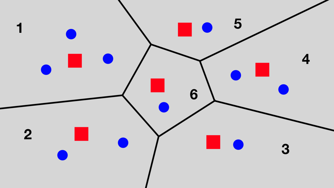
Math key and merge equations. Visual labels i, j, and * correspond to Pair selection uses the rate-weighted dissimilarity in eq. 7. The softmax-weighted merge (eq. 8) is
Appendix D THEORETICAL CHALLENGES: MORE DETAILS
The geometric picture above motivates the analytic tools below. We now detail three fundamental challenges in the statistical analysis of SGMoE that create substantial obstacles for parameter estimation and model selection:
(i) Softmax translation invariance. Gating parameters are identifiable only up to common translations. Unlike covariate-independent gating functions, the softmax gate is invariant under simultaneous shifts of intercepts and slopes, which makes the parameterization non-unique. As a result, standard identifiability arguments break down, and it becomes necessary to design translation-invariant loss functions. We address this by introducing the Voronoi partition and loss (see eq. 6), which takes an infimum over translations and thereby aligns the loss with the geometry of gating partitions.
(ii) Gate-expert PDE couplings. The likelihood function exhibits intrinsic gate-expert interactions that induce coupled differential relations among parameters. These relations lead to numerous linear dependencies among derivative terms in Taylor expansions, which prevents a direct decomposition of density discrepancies into independent components. Moreover, the parameters of the softmax gating numerators and the Gaussian experts are intrinsically linked through explicit PDEs,
| (13) |
where . Our analysis requires a systematic reorganization of these dependent terms to recover a meaningful set of independent directions.
(iii) Algebraic cancellations. Due to the tight coupling between numerators and denominators in the softmax-induced conditional density, higher-order cancellations in the expansions give rise to systems of polynomial equations introduced in eq. 3. The solvability of these systems determines the order of the first non-vanishing terms and directly controls the convergence rates of the MLE in over-specified models. This algebraic obstruction is a key source of non-standard, slower rates unique to SGMoE.
These challenges indicate that previously used loss functions, such as the Wasserstein distance, are insufficient for analyzing parameter quantities in either standard mixture models or mixtures with covariate-free gating functions. Moreover, the convergence rates of parameter estimates, as reported in Nguyen et al. (2023a), remain relatively slow due to the influence of the associated polynomial systems. Therefore, developing a dedicated method or algorithm, such as our DSC approach in Section 3, for models of this type is well motivated.
In addition, we also clarify the relationship between polynomial equations in eq. 3 and SGMoE in the over - specified case. Following Theorem 1, at , we can see that the convergence rate of Fast-Rate-Aware Voronoi distance is
this is an "optimal" rate for a mixing measure. However, the convergence rate of some parameters such as are not (following the definition of ). In particular, in the over-specified case, respectively , then the associated parameters suffer slower rates of the order or (see Table 1).
To explain this connection, we revisit our proof for over-specified case. Firstly, we want to show that because we can see that if we obtain this argument, we will get the "optimal" convergence rate of . We can rewrite the quantity as follows:
where we define and . Next, for each and , we denote and then apply the Taylor expansions to the functions and up to orders and (which we will choose later), respectively, as follows:
where and are Taylor remainders such that vanishes as for . As a result, the limit of when goes to infinity can be seen as a linear combination of elements of the following set:
which is shown to be linearly independent. By the Fatou’s lemma, we demonstrate that goes to zero as , implying that all the coefficients in the representation of , denoted by and , vanish when . Given that result, we aim to select the Taylor orders and such that at least one among the limits of and is different from zero, which leads to a contradiction. In the over-specified case, we assume that all the limits of and equal zero. After some steps of considering typical limits as in the previous setting which requires for all , we encounter the following system of polynomial equations:
for all such that and for some . Due to the construction of this system, it must have at least one non-trivial solution. Therefore, we choose for all .
To discuss about the value of with in general, by Fact 1, we obtain for and as increases, so does . Hence, we predict that . With this conjecture, we can see that the slow convergence rate of parameter estimation of SGMoE before we apply the merging atoms process.
Appendix E PROOF SKETCHES
In this section we expand the sketches for Lemma 1, Theorems 1, 2 and 3.
Why the loss in eq. 6?
When with , some Voronoi cells are multi-covered. The slow directions in (with exponents ) arise from these cells. augments with first-order merged-moment block-sums that vanish when a cell behaves as a single aggregate. Thus is simultaneously (i) exact-fit consistent, it reduces to when , and (ii) overfit-aware, penalizing precisely the slow directions that merging removes. In the over-specified case, cells with may persist; repeatedly merging atoms within such cells yields singletons and restores first-order behavior. Formally, using the density decomposition
we analyze the sums over indices with under ; for clarity, we also isolate the case , corresponding to . This leads directly to the merge operator and the aggregation path.
E.1 Proof Sketch of Lemma 1
We argue for the first merge ; the rest follows by induction. Assume . Then, for the Voronoi partition , there exist such that, for every ,
The minimizing pair of must lie in the same cell . Let the merged atom be as in eq. 8. Using the convexity of for and the identities implicit in eq. 8, we obtain the two key comparisons
The block-sum terms in also decrease since the merged parameters are softmax-weighted averages. Collecting terms yields , proving monotonicity.
E.2 Proof Sketch of Theorem 1
(A) Inverse bound.
We first prove an inverse inequality: there exists depending only on and such that, for any ,
| (14) |
The proof follows the density decomposition strategy in Nguyen et al. (2023a) but keeps all merged-moment block-sums that define . Let
A multi-index Taylor expansion (around within each cell ) up to order , together with the PDE identities and , rewrites as a linear combination of basis functions
with coefficients that are precisely the atomwise sums appearing in (up to constants). If eq. 14 failed, all these coefficients would have to vanish at a rate faster than , forcing a non-trivial solution to the polynomial system of eq. 3, in contradiction with the definition of (Fact 1). This yields eq. 14.
(B) Applying density rates.
E.3 Proof Sketch of Theorem 2
For , the height is the minimum -distance between any two atoms of . Inside a multi-covered cell , the Taylor/merged-moment analysis from the proof of eq. 14 implies that
The right-hand side is controlled by with the exponents , hence . For , heights converge at parametric rate because atoms are separated and .
E.4 Proof Sketch of Theorem 3
Let and . Under Condition K, a local Lipschitz/curvature argument yields
For , combine the inverse bound with and standard empirical-process bounds (e.g., van de Geer, 2000) to obtain . For , is exact/under-fit and converges at parametric rate, hence in probability.
Appendix F PROOF OF MAIN RESULTS
Before proving the main results, we fix notation used throughout this appendix. For any natural number , write . Given two sequences of positive real numbers and , we write (equivalently, ) to mean that there exists a constant such that for all . For a vector and any multi-index , set , , , and let denote its -norm; by default, refers to the -norm unless otherwise stated. We also use for the Frobenius norm of a matrix . For any set , denotes its cardinality. For two probability density functions and with respect to the Lebesgue measure , define as their total variation distance, while denotes the squared Hellinger distance. Moreover, for , , and a differentiable function of , we write the partial derivative of order as
Let be the parameter space. Write for the collection of discrete probability measures on with exactly atoms, and for those with at most atoms. For a mixing measure , we (slightly abusively) refer to each component as an “atom,” comprising both its weight and parameter . Finally, the domain of parameters in the SGMoE is , where . Furthermore, assume is compact and , the support of , is bounded. When clear from context, we drop and simply write and .
F.1 Proof of Lemma 1
We prove the inequality , and the rest are similar.
Assume that varies so that . We consider the Voronoi cells , for , of the mixing measure generated by the true components of . Since the argument in this proof is asymptotic, we assume without loss of generality that those Voronoi cells are independent of for all , i.e, .
Then, we have , and there exist and such that and for any and as approaches infinity.
We are going to show that the merging pair of indices must belong to a common . Indeed, for every pair in a common , since and , and and , we have
On the other hand, for every pair , where , because and , and and , we have
where the multiplicative constant is not dependent on . Hence, the merging pair must belong to a common .
Next, for any such that and still lie inside the domain of the parameter space , we define as
in which , , , , and .
We prove that . Let the merging pair of indices in the Voronoi cell , then and the merged atom is , i.e,
Hence, we have that
It follows that the term
Similarly, we can show that
To this end, we show the key convexity step in detail. Firstly, we define and () as follow:
Note that and and by the definition of the merged atom eq. 8, we have the convex combination identity .
By the fact that (since ), so we can use Jensen’s inequality (convexity of the map with ):
Multiply both sides by and substitute :
Analogously, we can show that
Combining the two inequalities above gives the claimed comparison between the contribution of the merged atom and the contributions of the two original atoms:
Hence
and therefore
F.2 Proof of Theorem 1
First of all, we study the convergence rate of the MLE of the SGMoE; that is, we will show the inverse bound for SGMoE. We revisit the following result on the identifiability of the SGMoE models, which was previously studied in Nguyen et al. (2023a); Jiang and Tanner (1999).
Fact 3 (Nguyen et al., 2023a, Proposition 1).
For any mixing measures and , if we have for almost surely , then it follows that and where for some and .
The identifiability of the softmax gating Gaussian mixture of experts guarantees that the MLE converges to the true mixing measure (up to the translation of the parameters in the softmax gating).
Given the consistency of the MLE, it is natural to ask about its convergence rate to the true parameters. Our next result establishes the convergence rate of conditional density estimation to the true conditional density , which lays an important foundation for the study of MLE’s convergence rate.
Fact 4 (Nguyen et al., 2023a, Proposition 2).
The density estimation converges to the true density under the Hellinger distance at the following rate:
That is,
where and are universal constants.
The result of Fact 4 indicates that under either the exact-specified or over-specified cases of the SGMoE, the rate of the conditional density function to the true one under Hellinger distance is of order (up to some logarithmic factors), which is parametric on the sample size.
Now, we establish the convergence rate of the MLE under the over-specified case of the SGMoE via the Fast-Rate-Aware Voronoi Distance .
Theorem 5.
Under the over-specified case of the SGMoE, namely, when , we obtain that
for any where is some universal constant depending only on and . Therefore, that lower bound leads to the following convergence rate of the MLE:
| (15) |
where and are some universal constants.
Proof of Theorem 5.
We are going to prove that there exists a constant depending only on and such that, for any ,
| (16) |
Then, by the Fact 4, we get the convergence rate of the MLE of SGMoE.
Local version: Firstly, we prove the local version of the eq. 16:
| (17) |
Assume that the inequality in eq. 17 does not hold true, there exists a sequence of mixing measures such that
when to infinity. Since the proof argument is asymptotic, we also assume that for all . Next, we consider the Voronoi cells , for , of the mixing measure generated by the true components of . And we can assume without loss of generality (WLOG) that those Voronoi cells are independent of for all , i.e. . Additionally, since , we have for any as . Furthermore, there exist and such that and as approaches infinity for any and . It suggests that we can upper bound as , where
in which , , , .
Step 1: Density Decomposition
In this step, we try to find a density decomposition for the quatity :
where we denote and .
Since each Voronoi cell possibly has more than one element, we continue to decompose as follows:
Now, we perform Taylor expansion up to the th order, and then rewrite with a note that as follows:
where is the remainder term such that
Next, for each and , we denote . By the partial differential equations
we have
Hence
It follows that
where .
Similarly, we can decompose by the first-order Taylor expansion as
where
Analogously, can be rewritten as
where
Therefore, can be represented as
| (18) |
with coefficients and are defined for any , and as
Step 2: Non-vanishing coefficients
Next, we will show that not all the quatities and go to as . We assume that all of them go to as . Then, by assumption , we have
| (19) |
For any such that , consider all implying , we have for all such that . Hence
| (20) |
Next, we consider such that and such that :
-
•
For , then
-
•
For , then
-
•
For , then
-
•
For , then
-
•
For , then
Combining the above limit and the formulation of together, it follows that
which implies that there exists some index such that and
for all . WLOG, we assume that . For such that , we have as . Thus, by dividing this ratio and the left hand side of the above equation and let , we have
| (21) |
for all such that .
Let us define and . Since the sequence is bounded, we can replace it by its subsequence that has a positive limit . Hence, at least one among , for , equals .
Similarly, we also define
Here, at least one of and for equals either or . Next, we divide both the numerator and the denominator of the ratio in eq. 21 by , and then achieve the following system of polynomial equations:
for all such that . However, based on the definition of , the above system has no non-trivial solutions, which is a contradiction. Thus, not all the quantities and go to as .
Step 3: Fatou’s lemma involvement
Following this, we define by be the maximum of the absolute values of those quantities. Based on the result in Step 2, we know that . Then, by applying the Fatou’s lemma, we obtain that
| (22) |
By assumption, the left-hand side of eq. 22 equals to , so the integrand in the right-hand side also equals to for almost surely . Hence, we get that as for almost surely . It follows from the decomposition of in eq. 18 that
for almost surely , where and denote the limits of and as , respectively, for all and . By definition, at least one among and is different from zero.
Furthermore, we denote the set as follows:
Fact 5 (Nguyen et al., 2023a, Lemma 2).
The set is linearly indeqendent w.r.t and , where is denoted as follows:
the set is linearly independent w.r.t and , it follows that
for all and , which is a contradiction. Hence, we achieve the eq. 17.
Global version: Hence, it is sufficient to prove its following global inequality:
| (23) |
Assume by contrary that there exists a sequence that satisfies
Then, we get that as . Since the set is compact, we can replace the sequence by its subsequence which converges to some mixing measure such that . Then, by the Fatou’s lemma, we get
It follows that
Thus, we obtain that for almost surely . By Fact 3, the mixing measure admits the form for some , where is some permutation of the set . It follows that , which contradicts the hypothesis . Hence, we obtain the inequality in eq. 16. ∎
Next, assume that with . From Fact 4, there exists a constant depending on and so that on an event, we call , with probability at least , we have
Now, we prove Theorem 1.
Proof of Theorem 1.
Firstly, we prove for the over-specified case. By Lemma 1 and Theorem 5, we have the first statement.
To prove the rest, we need to consider the exact-specified case. When , by definition of , we obtain that . Hence, by Lemma 1, we get the convergence rate
Assume that . Building on our previous work, there exist and such that for large enough, we get
for every , where , , and .
This implies that for every , by the triangle inequality, we have
Similarly, we have
Hence, we obtain that
| (24) |
Hence, on , the optimal choice of indices to merge for will be the same as for every large enough. It follows that we have two merged atoms are and denoted as follows:
and
After merging, we also have
| (25) |
and
Hence, . By the induction, we have the rest statement. ∎
F.3 Proof of Theorem 2
For the convergence rate of the height at all levels , from Theorem 1, we have
Because , by the pigeonhole principle, there exists at least two such that two atoms and belongs to a common Voronoi cell of some (we suppress the dependence of , and on for ease of notation). Hence,
Using the fact that , , and using the Hölder’s inequality, for every we have
Since the height of the dendrogram is the minimum of over all pairs , we obtain that
for all .
F.4 Proof of Theorem 3
Before we prove Theorem 3, we revisit preliminary on empirical process theory and connection between the Hellinger distance and the Wasserstein metric.
Preliminary on Empirical Process Theory.
Suppose . Denote is the empirical measure. Denote the empirical process for :
The following results is important in proof below.
Fact 6 (van de Geer, 2000, Theorem 5.11).
Let positive numbers satisfy:
and
then
Connection between the Hellinger distance and the Wasserstein metric.
We introduce the Wasserstein distances to measure the difference between two measures. For two mixing measure and , the Wasserstein- distance (for ) between and is defined as
| (26) |
where is the set of all couplings between and , i.e, . Fix , and consider such that , we obtain that
Now, we remind Lemma 1 in Ho and Nguyen (2016a).
Fact 7 (Ho and Nguyen, 2016a, Lemma 1).
Let denote a discrete probability measure and be the mixture density. According to the Lemma 1: Let such that both and are finite for some convex function . Then, .
By Fact 7, we can compare the expectation of Hellinger distance between and with the Wasserstein metric between and following:
Now, we are going to prove Theorem 3.
Proof of Theorem 3.
Firstly, we recall the empirical average log-likelihood and population average log-likelihood as follows:
where is the empirical measure from data, and the joint distribution over is then constructed by first sampling and then .
We divide into three cases.
Case 1: . For any , we denote by the distribution of . By the concavity of log function, we have
Therefore, for all we have
Hence,
Now, we compare Wasserstein metrics and . Since , with a note that for a probability , we have . Combining with all norms on finite space is equivalent, we obtain that
Then, we get . Using the fact that and , we also have
Let and denotes the bracketing entropy of under the Hellinger distance. By the Lemma 3 in Nguyen et al. (2023a), there is a constant such that for any .
Define, , substitute , , then for any positive number , we have and for large enough. Therefore, for large enough, we obtain that and
By Fact 6, we get
Combining with the bound on Hellinger distance, we have
For the second term, by the Chebyshev inequality, we have
| (27) |
Choose , we have
Hence, we conclude that
Case 2: . By the Theorem 1, we have
Assume that , since as , the Voronoi cell has only one element for any . WLOG, we suppose that for all . Moreover, there exist and independent of such that and as for all . By the definition of , we get for large enough
for every , where , , and .
Because the function satisfies Condition K (see Lemma 2), let , from condition K, there exist and such that
Besides, we can find constant and such that
Hence, we have
With the fact that is a convex function, we get
Therefore, we have
Hence
| (28) |
Now, we will bound the right-hand side of above equation, from Chebyshev inequality from eq. 27, choose , we get that
Obviously, the terms , thus there exist a constant such that . Then, for some constant , we have
Call the event under above case is , then we obtain that
approach when , where is defined in Section F.2. Therefore, combine both results, we can conclude that
Case 3: . Since for a measurable function for all , we can use uniform law of large number to get that
where means convergence in probability. Therefore,
We know that in probability, by application of Dominated Convergence theorem, we obtain
Combining the above results together, we get
∎
Checking condition K.
Finally, we check condition K for the function .
Lemma 2.
The condition K is satisfied for , where and are bounded as from the initial setup, and the eigenvalues of are bounded below and above by the positive constants and .
Proof of Lemma 2.
When with , by the equivalence of the norm, we can consider the cases where . We aim to show that for sufficiently small , there exist such that
which is equivalent to
Firstly, since is bounded, we can omit the term . Next, we note that
and if is bounded above and below far from 0 (which satisfies because is positive definite), then the map is Lipschitz; that is, there exists a constant such that
Furthermore, we have . Hence, for all , then we have
So that
We want to choose such that
Let , using the boundedness of , there exist such that
Hence, we only need to prove
which is equivalent to
We can bound the right-hand side of above equation as follow
Hence, it is sufficient to choose such that
Then .
Therefore, we complete the proof. ∎
F.5 Proof of Theorem 4
Define with (e.g., ). For , shrinks at order while the likelihood term cannot compensate at that scale given the chosen , so is suboptimal. For , the (under-fit) likelihood gap dominates and is worse than at . Hence in probability. We will give a more detailed proof below.