A non-asymptotic approach for model selection via penalization in high-dimensional mixture of experts models

TrungTin Nguyen; Hien D. Nguyen; Faicel Chamroukhi; Florence Forbes

Abstract

Mixture of experts (MoE) are a popular class of statistical and machine learning models that have gained attention over the years due to their flexibility and efficiency. In this work, we consider Gaussian-gated localized MoE (GLoME) and block-diagonal covariance localized MoE (BLoME) regression models to present nonlinear relationships in heterogeneous data with potential hidden graph-structured interactions between high-dimensional predictors. These models pose difficult statistical estimation and model selection questions, both from a computational and theoretical perspective. This paper is devoted to the study of the problem of model selection among a collection of GLoME or BLoME models characterized by the number of mixture components, the complexity of Gaussian mean experts, and the hidden block-diagonal structures of the covariance matrices, in a penalized maximum likelihood estimation framework. In particular, we establish non-asymptotic risk bounds that take the form of weak oracle inequalities, provided that lower bounds for the penalties hold. The good empirical behavior of our models is then demonstrated on synthetic and real datasets.

10.1214/154957804100000000

Keywords: [class=MSC] [; Primary ]62H30 62E17; [; ; secondary ]62H12

Keywords: Mixture of experts; linear cluster-weighted models; mixture of regressions; Gaussian locally-linear mapping models; clustering; oracle inequality; model selection; penalized maximum likelihood; block-diagonal covariance matrix; graphical Lasso;

1 Introduction

1.1 Mixture of experts models

Mixture of experts (MoE) models, originally introduced as neural network architectures in Jacobs et al. (1991); Jordan and Jacobs (1994), are flexible models that generalize the classical finite mixture models as well as finite mixtures of regression models (McLachlan and Peel, 2000, Sec. 5.13). Their flexibility comes from allowing the mixture weights (or the gating functions) to depend on the explanatory variables, along with the component densities (or experts). In the context of regression, MoE models with Gaussian experts and softmax or normalized Gaussian gating functions are the most popular choices and are powerful tools for modeling more complex nonlinear relationships between outputs (responses) and inputs (predictors) that arise from different subpopulations. The popularity of these conditional mixture density models arise largely due to their universal approximation properties, which have been studied in (Jiang and Tanner, 1999; Norets et al., 2010; Nguyen et al., 2016; Ho et al., 2019; Nguyen et al., 2019, 2021a), and which improve upon approximation capabilities of unconditional finite mixture models, as studied in (Genovese and Wasserman, 2000; Rakhlin et al., 2005; Nguyen, 2013; Ho et al., 2016a, b; Nguyen et al., 2020a, 2021b). Detailed reviews on the practical and theoretical aspects of MoE models can be found in Yuksel et al. (2012); Masoudnia and Ebrahimpour (2014); Nguyen and Chamroukhi (2018); Nguyen (2021).

In this paper, we wish to investigate MoE models with Gaussian experts and normalized Gaussian gating functions for clustering and regression, first introduced by Xu et al. (1995), which extended the original MoE models of Jacobs et al. (1991). From hereon in, we refer to these models as Gaussian-gated localized MoE (GLoME) models and block-diagonal covariance for localized MoE (BLoME) models, and we provide their precise definitions in Section 2.1. Furthermore, the original MoE models with softmax gating functions will be referred to as linear-combination-of-bounded-functions softmax-gated MoE (LinBoSGaME) regression models. In particular, we simply refer to affine instances of LinBoSGaME models as softmax-gated MoE (SGaME) regression models. It is worth pointing out that the BLoME models generalize GLoME models by utilizing a parsimonious covariance structure, via block-diagonal structures for covariance matrices in the Gaussian experts. It is also interesting to point out that supervised Gaussian locally-linear mapping (GLLiM) and block-diagonal covariance for Gaussian locally-linear mapping (BLLiM) models in Deleforge et al. (2015a) and Devijver et al. (2017) are affine instances of GLoME and BLoME models, respectively, where the latter pair consider general linear combination of bounded functions instead of affine for mean functions of Gaussian experts, in the prior pair.

One of the main disadvantages of LinBoSGaME models is the difficulty of applying an expectation–maximization (EM) algorithm (Dempster et al., 1977; McLachlan and Krishnan, 1997), which requires an internal iterative numerical optimization procedure (e.g., iteratively-reweighted least squares, Newton-Raphson algorithm) to update the softmax parameters. To overcome this problem, we instead use the Gaussian gating network that enables us to link BLoME with hierarchical Gaussian mixture model. Then, the maximization with respect to the parameters of the gating network can be solved analytically with the EM algorithm framework, which decreases the computational complexity of the estimation routine. Furthermore, we can then also make use of well-established theoretical results for finite mixture models.

We note here that both GLoME and BLoME models have been thoroughly studied in the statistics and machine learning literatures in many different guises, including localized MoE (Ramamurti and Ghosh, 1996, 1998; Moerland, 1999; Bouchard, 2003), normalized Gaussian networks (Sato and Ishii, 2000), MoE modeling of priors in Bayesian nonparametric regression (Norets and Pelenis, 2014; Norets and Pati, 2017), cluster-weighted modeling (Ingrassia et al., 2012), deep mixture of linear inverse regressions (Lathuilière et al., 2017), hierarchical Gaussian locally linear mapping structured mixture (HGLLiM) model (Tu et al., 2019), multiple-output Gaussian gated mixture of linear experts (Nguyen et al., 2019), and approximate Bayesian computation with surrogate posteriors using GLLiM (Forbes et al., 2021).

1.2 Goals

Our main goal is to learn potentially nonlinear relationships between a multivariate output and a high-dimensional input issued from a heterogeneous population. This involves performing regression, clustering and model selection, simultaneously. While estimation can be performed using standard EM algorithms, it crucially depends and requires data-driven hyperparameter choices, including the number of mixture components (or clusters), the degree of complexity of each Gaussian expert’s mean function, and the hidden block-diagonal structures of the covariance matrices. Recall that hyperparameter choices of data-driven learning algorithms belong to the class of model selection problems, which have attracted a lot of attention in statistics and machine learning over the past 50 years (Akaike, 1974; Mallows, 1973; Anderson and Burnham, 2002; Massart, 2007; Arlot, 2019). Specifically, given a set of models, how do we select the one with the lowest possible risk from the data? Note that penalization is one of the main strategies proposed for model selection. It suggests choosing the estimator that minimizes the sum of its empirical risk and some penalty terms corresponding to the fit of the model to the data while avoiding overfitting.

1.3 Related literature

In general, model selection for MoE models is often performed using the Akaike information criterion (AIC) (Akaike, 1974), the Bayesian information criterion (BIC) (Schwarz et al., 1978) or the BIC-like approximation of integrated classification likelihood (ICL-BIC) Biernacki et al. (2000). An important limitation of these criteria, however, is that they are only valid asymptotically. This implies that there is no finite-sample guarantee when using AIC, BIC or ICL-BIC, to choose between different levels of complexity. Their use in small samples is, therefore, ad hoc. To overcome such difficulties, Birgé and Massart (2007) proposed a novel approach, called the slope heuristics, supported by a non-asymptotic oracle inequality. This method leads to an optimal data-driven choice of multiplicative constants for the penalties. Recent reviews and practical issues concerning the slope heuristic can be found in Baudry et al. (2012); Arlot (2019) and the references given therein.

It should be emphasized that a general model selection result, originally established by (Massart, 2007, Theorem 7.11), ensures a penalized criterion leads to a good model selection and that the penalty is known only up to multiplicative constants and is proportional to the dimensions of models. In particular, these multiplicative constants can be calibrated by the slope heuristic approach in a finite-sample setting. Then, in the spirit of the methods based on concentration inequalities developed in Massart (2007); Massart and Meynet (2011); Cohen and Le Pennec (2011, 2013), a number of finite-sample oracle type inequalities have been established for the least absolute shrinkage and selection operator (LASSO) (Tibshirani, 1996) and general penalized maximum likelihood estimators (PMLE). These results include the works for high-dimensional Gaussian graphical models (Devijver and Gallopin, 2018), Gaussian mixture model selection (Maugis and Michel, 2011a, b; Maugis-Rabusseau and Michel, 2013), finite mixture regression models (Meynet, 2013; Devijver, 2015a, b, 2017a, 2017b), and LinBoSGaME models, outside the high-dimensional setting (Montuelle et al., 2014).

1.4 Main contributions

To the best of our knowledge, no attempt has been made in the literature to develop a finite-sample oracle inequality for the framework of MoE regression models for high-dimensional data. In this paper, our first original contribution is to provide finite-sample oracle inequalities, Theorems 3.3 and 3.4 for high-dimensional GLoME and BLoME models, respectively. More specifically, we establish non-asymptotic risk bounds that take the form of weak oracle inequalities, provided that the lower bounds on the penalties are true, in high-dimensional GLoME and BLoME models, based on an inverse regression strategy and block-diagonal structures of the Gaussian covariance matrices experts. Unlike traditional criteria such as AIC, BIC, or ICL-BIC, which are based on asymptotic theory or a Bayesian approach, our contributed non-asymptotic risk bounds allow the number $n$ of observations to be fixed while the dimensionality and cardinality of the models, characterized by the number of covariates and the size of the response, are allowed to grow with respect to $n$ and can be much larger than $n$ .

In particular, our oracle inequalities show that the Jensen–Kullback–Leibler loss performance of our PMLEs is comparable to that of oracle models if we take sufficiently large constants in front of the penalties, whose shapes are only known up to multiplicative constants and proportional to the dimensions of the models. These theoretical justifications for the shapes of the penalties motivate us to make use of the slope heuristic criterion to select several hyperparameters, including the number of mixture components, the degree of polynomial mean functions, and the potential hidden block-diagonal structures of the covariance matrices of the multivariate predictors.

Moreover, in Theorem 3.3, we extends a corollary of (Montuelle et al., 2014, Theorem 1), which can be verified via Lemma 1 from Nguyen et al. (2021a), which makes explicit the relationship between softmax and Gaussian gating classes.

Another significant contribution is the numerical experiments for simulated and real data sets in Section 5 that support our theoretical results, and the statistical study of non-asymptotic model selection in GLoME models. To the best of our knowledge, instead of using classical asymptotic approaches for model selection such as AIC, BIC and ICL-BIC, we are the first to illustrate that the slope heuristic works well for MoEs with Gaussian experts and normalized Gaussian gating networks such as GLLiM, BLLiM, GLoME, and BLoME models. Note that our main objective here is to investigate how well the empirical tensorized Kullback–Leibler divergence between the true model ( $s_{0}^{*}$ ) and the selected model $\hat{s}_{\hat{𝐦}}^{*}$ follows the finite-sample oracle inequality of Theorem 3.3, as well as the convergence rate $𝒪 (n^{- 1})$ of the error upper bound. Therefore, we focus on $1$ -dimensional data sets. Beyond the statistical estimation and model selection purposes considered here, the dimensionality reduction capability of GLLiM and BLLiM models in high-dimensional regression data, can be found in (Deleforge et al., 2015a, Section 6) and (Devijver et al., 2017, Sections 3 and 4), respectively.

Specifically, besides the important theoretical issues regarding the tightness of upper bounds, how to integrate a priori information, and a minimax analysis of our proposed PMLEs, our finite-sample oracle inequalities and the corresponding illustrative numerical experiments help to partially answer the following two important questions raised in the field of MoE regression models: (1) What is the number of mixture components $K$ to choose, given the sample size $n$ ; and (2) Whether it is better to use a few complex experts or a combination of many simple experts, given the total number of parameters. Note that such problems are also considered in the work of (Mendes and Jiang, 2012, Proposition 1), where the authors provided some qualitative guidance and only suggested a practical method for choosing $K$ and $d$ , involving a complexity penalty or cross-validation. Furthermore, their model is only non-regularized maximum-likelihood estimation, and thus is not suitable for the high-dimensional setting.

Lastly, we emphasize that although the finite-sample oracle inequalities compare performances of our estimators with the best model in the collection, they also allow us to approximate a rich class of conditional densities if we take enough clusters and/or a high enough degree $d$ of polynomials in the mean of the functions of Gaussian experts, in the context of mixture of Gaussian experts (Jiang and Tanner, 1999; Mendes and Jiang, 2012; Nguyen et al., 2016; Ho et al., 2019; Nguyen et al., 2021a). This leads to the upper bounds of the risks being small.

1.5 Main challenges

For the Gaussian gating parameters, the technique for handling the logistic weights in the SGaME models of Montuelle et al. (2014) is not directly applicable to the GLoME or BLoME framework, due to the quadratic form of the canonical link. Therefore, we have to propose a reparameterization trick¹¹1Note that we only use this nomenclature to perform a change of variables of the Gaussian gating parameters space of GLoME models via the logistic weights of SGaME models. This reparameterization trick does not stand for the well-known one of variational autoencoders (VAEs) in deep learning literature (see Kingma and Welling (2013), for more details). to bound the metric entropy of the Gaussian gating parameters space; see (4.1.3) and Lemma 4.9 for more details.

To work with conditional density estimation in the BLLiM and BLoME models, it is natural to make use of a general conditional density model selection theorem from Cohen and Le Pennec (2011, 2013), see also Theorem 4.5 for its adaption to our context. However, it is worth mentioning that since the collection of models constructed by the BLLiM model Devijver et al. (2017) or by some appropriate procedures for BLoME models in practice is usually random, we have to utilize a model selection theorem for MLE among a random subcollection (cf. (Devijver, 2015b, Theorem 5.1) and (Devijver and Gallopin, 2018, Theorem 7.3)).

In particular, our collections of BLoME models must satisfy certain regularity assumptions, see Section 4.2.3 for details, which are not easy to verify due to the complexity of BLoME models and technical reasons. For BLoME models, the main difficulty in proving our oracle inequality lies in bounding the bracketing entropy of the Gaussian gating functions and Gaussian experts with block-diagonal covariance matrices. To solve the first problem, we need to use our previous trick of reparametrizing the Gaussian gating parameter space. For the second one, based on some ideas of Gaussian mixture models from Genovese and Wasserman (2000); Maugis and Michel (2011a), we provide a novel extension for standard MoE models with Gaussian gating networks. Note that our important contributions also extend the recent result on block-diagonal covariance matrices in Devijver and Gallopin (2018), which is only developed for Gaussian graphical models.

In addition, there are two possible ways to decompose the bracketing entropy of collection models based on different distances. As mentioning in Appendix B.2.1 from Montuelle et al. (2014), their decomposition boils down to assuming that the predictor domain is bounded. And this limiting assumption can then be relaxed by using a smaller distance, namely a tensorized extension of the Hellinger distance $d^{\otimes n}$ in (2.24), but bounding the corresponding bracketing entropy becomes much more difficult. Nevertheless, it is important to point out that we are able to weaken this limiting assumption by using the smaller distance: $d^{\otimes n}$ , for the bracketing entropy of our collection of BLoME models, see Lemma 4.14 for more details. This reinforces our original contributions concerning the control of bracketing entropy of BLoME models.

1.6 Organization

The rest of this paper is organized as follows. In Section 2, we present the notation and framework for GLoME, and BLoME models and their special cases, GLLiM, and BLLiM models. In Section 3, we state the main results of this paper: finite-sample oracle inequalities satisfied by the PMLEs. Section 4 is devoted to the proofs and main mathematical challenges in establishing our new finite-sample oracle inequalities. We experimentally evaluate our new results in simulated and real datasets in Section 5. Some conclusions and perspectives are provided in Section 6. The proofs of technical lemmas can be found in Appendix A.

2 Notation and framework

From now on, for any $L \in ℕ^{⋆}$ , we write $[L]$ to denote the set ${1, \dots, L}$ . We are interested in estimating the law of the random variable $𝐘 = (𝐘_{j})_{j \in [L]}$ , conditionally on $𝐗 = (𝐗_{j})_{j \in [D]}$ . Here and subsequently, given any $n \in ℕ^{⋆}$ , $(𝐗_{[n]}, 𝐘_{[n]}) : = (𝐗_{i}, 𝐘_{i})_{i \in [n]}$ denotes a random sample, and $𝐱$ and $𝐲$ stands for the observed values of the random variables $𝐗$ and $𝐘$ , respectively. The following assumptions will be needed throughout the paper. We assume that the covariates $𝐗$ are independent but not necessarily identically distributed. The assumptions on the responses $𝐘$ are stronger: conditional on $𝐗_{[n]}$ , $𝐘_{[n]}$ are independent, and each $𝐘$ follows a law with true (but unknown) PDF $s_{0} (\cdot ∣ 𝐗 = 𝐱)$ , which is approximated via MoE models. For a matrix $𝐀$ , let $m (𝐀)$ and $M (𝐀)$ be, respectively, the modulus of the smallest and largest eigenvalues of $𝐀$ .

2.1 GLoME and BLoME models

Motivated by an inverse regression framework, where the role of predictor and response variables will be exchanged such that $𝐘$ becomes the input and $𝐗$ plays the role of a multivariate output, we consider GLoME and BLoME models with inverse conditional probability density functions (PDFs) of the form (2.1). This construction goes back to the work of Li (1991); Xu et al. (1995); Deleforge et al. (2015a); Perthame et al. (2018), and is very useful in a high-dimensional regression context, where typically $D ≫ L$ . In this way, we define PDF of $𝐗$ conditional on $𝐘 = 𝐲$ as follows:

	$s_{𝝍_{K, d}} (𝐱 ∣ 𝐲)$	$= \sum_{k = 1}^{K} g_{k} (𝐲; 𝝎) ϕ_{D} (𝐱; 𝝊_{k, d} (𝐲), 𝚺_{k}),$		(2.1)
	$g_{k} (𝐲; 𝝎)$	$= \frac{π_{k} ϕ_{L} (𝐲; 𝐜_{k}, 𝚪_{k})}{\sum_{j = 1}^{K} π_{j} ϕ_{L} (𝐲; 𝐜_{j}, 𝚪_{j})} \cdot$		(2.2)

Here, $g_{k} (\cdot; 𝝎)$ and $ϕ_{D} (\cdot; 𝝊_{k, d} (\cdot), 𝚺_{k})$ , $k \in [K]$ , $K \in ℕ^{⋆}$ , $d \in ℕ^{⋆}$ , are called normalized Gaussian gating functions (or Gaussian gating networks) and Gaussian experts, respectively. Furthermore, we decompose the parameters of the model as follows: $𝝍_{K, d} = (𝝎, 𝝊_{d}, 𝚺) \in 𝛀_{K} \times 𝚼_{K, d} \times 𝐕_{K} = : 𝚿_{K, d}$ , $𝝎 = (𝝅, 𝒄, 𝚪) \in (𝚷_{K - 1} \times 𝐂_{K} \times 𝑽^{'}_{K}) = : 𝛀_{K}$ , $𝝅 = (π_{k})_{k \in [K]}$ , $𝒄 = (𝐜_{k})_{k \in [K]}$ , $𝚪 = (𝚪_{k})_{k \in [K]}$ , $𝝊_{d} = (𝝊_{k, d})_{k \in [K]} \in 𝚼_{K, d}$ , and $𝚺 = (𝚺_{k})_{k \in [K]} \in 𝐕_{K}$ . Note that $𝚷_{K - 1} = {(π_{k})_{k \in [K]} \in (ℝ^{+})^{K}, \sum_{k = 1}^{K} π_{k} = 1}$ is a $K - 1$ dimensional probability simplex, $𝐂_{K}$ is a set of $K$ -tuples of mean vectors of size $L \times 1$ , $𝑽^{'}_{K}$ is a set of $K$ -tuples of elements in $𝒮_{L}^{+ +}$ , where $𝒮_{L}^{+ +}$ denotes the collection of symmetric positive definite matrices on $ℝ^{L}$ , $𝚼_{K, d}$ is a set of $K$ -tuples of mean functions from $ℝ^{L}$ to $ℝ^{D}$ depending on a degree $d$ (e.g., a degree of polynomials), and $𝐕_{K}$ is a set containing $K$ -tuples from $𝒮_{D}^{+ +}$ .

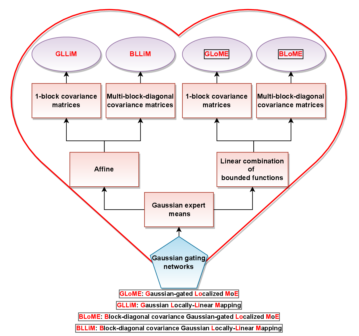
Recall that GLLiM and BLLiM models are affine instances of GLoME and BLoME models, and are especially useful for high-dimensional regression data, since there exist link functions between the inverse and forward conditional density; see Figure 1 for comprehensive classification and nomenclature of standard MoE regression models with Gaussian gating networks. Note that the principle of inverse regression is only useful when the functions $𝝊_{k, d} (𝐲)$ are linear, because there is no explicit way to express the law of $𝐘 ∣ 𝐗$ from that of $𝐗 ∣ 𝐘$ for higher degree of polynomials. However, to have more consistent notations with the previous affine results of GLLiM, BLLiM models from Deleforge et al. (2015a); Devijver et al. (2017), we decide to use the inverse regression frameworks instead of the forward one.

Refer to caption — Figure 1: A comprehensive classification and nomenclature of standard MoE regression models with Gaussian gating networks.

In the BLoME model, we wish to make use of block-diagonal covariance structures by replacing $𝚺_{k}$ and $𝐕_{K}$ with $𝚺_{k} (𝐁_{k})$ and $𝐕_{K} (𝐁)$ , defined in (2.5), respectively (see, e.g., (Devijver et al., 2017; Devijver and Gallopin, 2018)). This block-diagonal structures for covariance matrices are not only used to trade-off between complexity and sparsity but is also motivated by some real applications, where we want to perform prediction on data sets with heterogeneous observations and hidden graph-structured interactions between covariates; for instance, for gene expression data sets in which conditionally on the phenotypic response, genes interact with few other genes only, i.e., there are small modules of correlated genes (see (Devijver et al., 2017; Devijver and Gallopin, 2018) for more details). To be more precise, for $k \in [K]$ , we decompose $𝚺_{k} (𝐁_{k})$ into $G_{k}$ blocks, $G_{k} \in ℕ^{⋆}$ , and we denote by $d^{[g]}_{k}$ the set of variables into the $g$ th group, for $g \in [G_{k}]$ , and by $c a r d (d^{[g]}_{k})$ the number of variables in the corresponding set. Then, we define $𝐁_{k} = (d^{[g]}_{k})_{g \in [G_{k}]}$ to be a block structure for the cluster $k$ , and $𝐁 = (𝐁_{k})_{k \in [K]}$ to be the covariate indexes into each group for each cluster. In this way, to construct the block-diagonal covariance matrices, up to a permutation, we make the following definition: $𝐕_{K} (𝐁) = (𝐕_{k} (𝐁_{k}))_{k \in [K]}$ , for every $k \in [K]$ ,

𝐕_{k} (𝐁_{k}) = {𝚺_{k} (𝐁_{k}) \in 𝒮_{D}^{+ +} | \begin{matrix} 𝚺_{k} (𝐁_{k}) = 𝐏_{k} (\begin{matrix} 𝚺_{k}^{[1]} & 𝟎 & \dots & 𝟎 \\ 𝟎 & 𝚺_{k}^{[2]} & \dots & 𝟎 \\ 𝟎 & 𝟎 & ⋱ & 𝟎 \\ 𝟎 & 𝟎 & \dots & 𝚺_{k}^{[G_{k}]} \end{matrix}) 𝐏^{- 1}_{k}, \\ 𝚺_{k}^{[g]} \in 𝒮^{+ +}_{c a r d (d^{[g]}_{k})}, \forall g \in [G_{k}] \end{matrix}} .

(2.5)

Here, $𝐏_{k}$ corresponds to the permutation leading to a block-diagonal matrix in cluster $k$ . It is worth pointing out that outside the blocks, all coefficients of the matrix are zeros and we also authorize reordering of the blocks: e.g., ${(1, 3); (2, 4)}$ is identical to ${(2, 4); (1, 3)}$ , and the permutation inside blocks: e.g., the partition of $4$ variables into blocks ${(1, 3); (2, 4)}$ is the same as the partition ${(3, 1); (4, 2)}$ .

It is interesting to point out that the BLLiM framework aims to model a sample of high-dimensional regression data issued from a heterogeneous population with hidden graph-structured interaction between covariates. In particular, the BLLiM model is considered as a good candidate for performing model-based clustering and for predicting the response in situations affected by the “curse of dimensionality” phenomenon, where the number of parameters could be larger than the sample size. Indeed, to deal with high-dimensional regression problems, the BLLiM model is based on an inverse regression strategy, which inverts the role of the high-dimensional predictor and the multivariate response. Therefore, the number of parameters to estimate is drastically reduced. More precisely, BLLiM utilizes GLLiM, described in Deleforge et al. (2015b, a), in conjunction with a block-diagonal structure hypothesis on the residual covariance matrices, to make a trade-off between complexity and sparsity. This prediction model is fully parametric and highly interpretable. For instance, it can be used for the analysis of transcriptomic data in molecular biology to classify observations or predict phenotypic states; see e.g., (Golub et al., 1999; Nguyen and Rocke, 2002; Lê Cao et al., 2008). Indeed, if the predictor variables are gene expression data measured by microarrays or by the RNA-seq technologies, and the response is a phenotypic variable, the BLLiM model not only provides clusters of individuals based on the relation between gene expression data and the phenotype, but also implies a gene regulatory network specific to each cluster of individuals (see (Devijver et al., 2017) for more details).

In order to establish our finite-sample oracle inequalities, Theorems 3.3 and 3.4, we need to explicitly impose some classical boundedness conditions on the parameter space.

2.1.1 Gaussian gating networks

We shall restrict our study to bounded Gaussian gating parameter vectors. Specifically, we assume that there exist deterministic positive constants $a_{𝝅}, A_{𝒄}, a_{𝚪}, A_{𝚪}$ , such that $𝝎$ belongs to $\tilde{𝛀}_{K}$ , where

	$\tilde{𝛀}_{K}$	$= {𝝎 \in 𝛀_{K} : \forall k \in [K], ∥ 𝐜_{k} ∥_{\infty} \leq A_{𝒄},$
		$a_{𝚪} \leq m (𝚪_{k}) \leq M (𝚪_{k}) \leq A_{𝚪}, a_{𝝅} \leq π_{k}} .$		(2.6)

2.1.2 Gaussian experts

Following the same structure for the Gaussian mean experts from Montuelle et al. (2014), the set $𝚼_{K, d}$ will be chosen as a tensor product of compact sets of moderate dimension (e.g., a set of polynomials of degree smaller than $d$ , whose coefficients are smaller in absolute values than $T_{𝚼}$ ). Then, $𝚼_{K, d}$ is defined as a linear combination of a finite set of bounded functions whose coefficients belong to a compact set. This general setting includes polynomial bases when the covariates are bounded, Fourier bases on an interval, as well as suitably renormalized wavelet dictionaries. More specifically, $𝚼_{K, d} = \otimes_{k \in [K]} 𝚼_{k, d} = : 𝚼_{k, d}^{K}$ , where $𝚼_{k, d} = 𝚼_{b, d}$ , $\forall k \in [K]$ , and

𝚼_{b, d}

= {𝐲 \mapsto (\sum_{i = 1}^{d} 𝜶_{i}^{(j)} φ_{𝚼, i} (𝐲))_{j \in [D]} = : (𝝊_{d, j} (𝐲))_{j \in [D]} : ∥ 𝜶 ∥_{\infty} \leq T_{𝚼}} .

(2.7)

Here, the subscript $b$ stands for ”bounded functions”, $d \in ℕ^{⋆}, T_{𝚼} \in ℝ^{+}$ , and $(φ_{𝚼, i})_{i \in [d]}$ is a collection of bounded functions on $𝒴$ . In particular, we focus on the bounded $𝒴$ case and assume that $𝒴 = [0, 1]^{L}$ , without loss of generality. In this case, $φ_{𝚼, i}$ can be chosen as monomials with maximum (non-negative) degree $d$ : $𝐲^{𝐫} = \prod_{l = 1}^{L} 𝐲^{𝐫_{l}}_{l}$ . Recall that a multi-index $𝐫 = (𝐫_{l})_{l \in [L]}, 𝐫_{l} \in ℕ^{⋆} \cup {0}, \forall l \in [L]$ , is an $L$ -tuple of nonnegative integers. We define $| 𝐫 | = \sum_{l = 1}^{L} 𝐫_{l}$ and the number $| 𝐫 |$ is called the order or degree of $𝐲^{𝐫}$ . Then, $𝚼_{K, d} = 𝚼_{p, d}^{K}$ , where

𝚼_{p, d}

= {𝐲 \mapsto (\sum_{| 𝐫 | = 0}^{d} 𝜶_{𝐫}^{(j)} 𝐲^{𝐫})_{j \in [D]} = : (𝝊_{d, j} (𝐲))_{j \in [D]} : ∥ 𝜶 ∥_{\infty} \leq T_{𝚼}} .

(2.8)

Here, the subscript $p$ stands for ”polynomial”.

For GLoME models, note that any covariance matrix $𝚺_{k}$ can be decomposed into the form $B_{k} 𝐏_{k} 𝐀_{k} 𝐏_{k}^{⊤}$ , such that $B_{k} = | 𝚺_{k} |^{1 / D}$ is a positive scalar corresponding to the volume, $𝐏_{k}$ is the matrix of eigenvectors of $𝚺_{k}$ and $𝐀_{k}$ the diagonal matrix of normalized eigenvalues of $𝚺_{k}$ ; $B_{-} \in ℝ^{+}, B_{+} \in ℝ^{+}$ , $𝒜 (λ_{-}, λ_{+})$ is a set of diagonal matrices $𝐀_{k}$ , such that $| 𝐀_{k} | = 1$ and $\forall i \in [D], λ_{-} \leq (𝐀_{k})_{i, i} \leq λ_{+}$ , where $λ_{-}, λ_{+} \in ℝ$ ; and $S O (D)$ is the special orthogonal group of dimension $D$ . In this way, we obtain what is known as the classical covariance matrix sets described by Celeux and Govaert (1995) for Gaussian parsimonious clustering models, defined by

	$𝐕_{K}$	$= {(B_{k} 𝐏_{k} 𝐀_{k} 𝐏_{k}^{⊤})_{k \in [K]} : \forall k \in [K], B_{-} \leq B_{k} \leq B_{+},$
		$𝐏_{k} \in S O (D), 𝐀_{k} \in 𝒜 (λ_{-}, λ_{+})} .$		(2.9)

For the block-diagonal covariances of Gaussian experts from BLoME models, we assume that there exist some positive constants $λ_{m}$ and $λ_{M}$ such that, for every $k \in [K]$ ,

	$\tilde{𝐕}_{K} (𝐁)$	$= {(𝚺_{k} (𝐁_{k}))_{k \in [K]} \in 𝐕_{K} (𝐁) :$
		$0 < λ_{m} \leq m (𝚺_{k} (𝐁_{k})) \leq M (𝚺_{k} (𝐁_{k})) \leq λ_{M}} .$		(2.10)

Note that this is a typical assumption and is also used in the block-diagonal covariance selection for Gaussian graphical models of Devijver and Gallopin (2018).

Next, characterizations of GLLiM and BLLiM models are provided in Section 2.2.

2.2 High-dimensional regression via GLLiM and BLLiM models

The GLLiM and BLLiM models, as originally introduced in Deleforge et al. (2015a); Devijver et al. (2017), are used to capture the nonlinear relationship between the response and the set of covariates from a high-dimensional regression data, imposed by a potential hidden graph structured interaction, typically in the case when $D ≫ L$ , by the $K$ locally affine mappings:

𝐘 = \sum_{k = 1}^{K} 𝕀 (Z = k) (𝐀^{*}_{k} 𝐗 + 𝐛^{*}_{k} + 𝐄^{*}_{k}) .

(2.11)

Here, $𝕀$ is an indicator function and $Z$ is a latent variable capturing a cluster relationship, such that $Z = k$ if $𝐘$ originates from cluster $k \in [K]$ . Cluster specific affine transformations are defined by matrices $𝐀^{*}_{k} \in ℝ^{L \times D}$ and vectors $𝐛^{*}_{k} \in ℝ^{L}$ . Furthermore, $𝐄^{*}_{k}$ are error terms capturing both the reconstruction error due to the local affine approximations and the observation noise in $ℝ^{L}$ .

Following the common assumption that $𝐄^{*}_{k}$ is a zero-mean Gaussian variable with covariance matrix $𝚺_{k}^{*} \in ℝ^{L \times L}$ , it holds that

p (𝐘 = 𝐲 ∣ 𝐗 = 𝐱, Z = k; 𝝍^{*}_{K}) = Φ_{L} (𝐲; 𝐀^{*}_{k} 𝐱 + 𝐛^{*}_{k}, 𝚺^{*}_{k}),

(2.12)

where we denote by $𝝍^{*}_{K}$ the vector of model parameters and $Φ_{L}$ is the PDF of a Gaussian distribution of dimension $L$ . In order to allow the affine transformations to be local, $𝐗$ is defined as a mixture of $K$ Gaussian components as follows:

p (𝐗 = 𝐱 ∣ Z = k; 𝝍^{*}_{K}) = Φ_{D} (𝐱; 𝐜^{*}_{k}, 𝚪^{*}_{k}), p (Z = k; 𝝍^{*}_{k}) = 𝝅^{*}_{k},

(2.13)

where $𝐜^{*}_{k} \in ℝ^{D}, 𝚪^{*}_{k} \in ℝ^{D \times D}$ , $𝝅^{*} = (𝝅^{*}_{k})_{k \in [K]} \in 𝚷^{*}_{K - 1}$ , and $𝚷^{*}_{K - 1}$ is the $K - 1$ dimensional probability simplex. Then, according to formulas for conditional multivariate Gaussian variables and the following hierarchical decomposition

p (𝐘 = 𝐲, 𝐗 = 𝐱; 𝝍^{*}_{K})

= \sum_{k = 1}^{K} 𝝅^{*}_{k} Φ_{D} (𝐱; 𝐜^{*}_{k}, 𝚪^{*}_{k}) Φ_{L} (𝐲; 𝐀^{*}_{k} 𝐱 + 𝐛^{*}_{k}, 𝚺^{*}_{k}),

we obtain the following forward conditional density (Deleforge et al., 2015a):

p (𝐘 = 𝐲 ∣ 𝐗 = 𝐱; 𝝍^{*}_{K}) = \sum_{k = 1}^{K} \frac{𝝅^{*}_{k} Φ_{D} (𝐱; 𝐜^{*}_{k}, 𝚪^{*}_{k})}{\sum_{j = 1}^{K} 𝝅^{*}_{j} Φ_{D} (𝐱; 𝐜^{*}_{j}, 𝚪^{*}_{j})} Φ_{L} (𝐲; 𝐀^{*}_{k} 𝐱 + 𝐛^{*}_{k}, 𝚺^{*}_{k}),

(2.14)

where $𝝍^{*}_{K} = (𝝅^{*}, 𝜽^{*}_{K}) \in Π_{K - 1} \times 𝚯^{*}_{K} = : 𝚿^{*}_{K}$ . Here, $𝜽^{*}_{K} = (𝐜^{*}_{k}, 𝚪^{*}_{k}, 𝐀^{*}_{k}, 𝐛^{*}_{k}, 𝚺^{*}_{k})_{k \in [K]}$ and

𝚯^{*}_{K} = (ℝ^{D} \times 𝒮_{D}^{+ +} (ℝ) \times ℝ^{L \times D} \times ℝ^{L} \times 𝒮_{L}^{+ +} (ℝ))^{K} .

Without assuming anything on the structure of parameters, the dimension of the model, denoted by $dim (\cdot)$ , is defined as the total number of parameters that has to be estimated, as follows:

dim (𝚿^{*}_{K}) = K (1 + D (L + 1) + \frac{D (D + 1)}{2} + \frac{L (L + 1)}{2} + L) - 1 .

It is worth mentioning that $dim (𝚿_{K})$ is typically very large compared to the sample size (see, e.g., Deleforge et al. (2015a); Devijver et al. (2017); Perthame et al. (2018) for more details in their real data sets) whenever $D$ is large and $D ≫ L$ . Furthermore, it is more realistic to make assumption on the residual covariance matrices $𝚺^{*}_{k}$ of error vectors $𝐄^{*}_{k}$ rather than on $𝚪^{*}_{k}$ (cf. (Deleforge et al., 2015a, Section 3)). This justifies the use of the inverse regression trick from Deleforge et al. (2015a), which leads a drastic reduction in the number of parameters to be estimated.

More specifically, in (2.14), the roles of input and response variables were exchanged such that $𝐘$ becomes the covariates and $𝐗$ plays the role of the multivariate response. Therefore, its corresponding inverse conditional density is defined as a Gaussian locally-linear mapping (GLLiM) model, based on the previous hierarchical Gaussian mixture model, as follows:

$p (Z = k; 𝝍_{k})$	$= π_{k},$	(2.15)
$p (𝐘 = 𝐲 ∣ Z = k; 𝝍_{K})$	$= Φ_{L} (𝐲; 𝐜_{k}, 𝚪_{k}),$	(2.16)
$p (𝐗 = 𝐱 ∣ 𝐘 = 𝐲, Z = k; 𝝍_{K})$	$= Φ_{D} (𝐱; 𝐀_{k} 𝐲 + 𝐛_{k}, 𝚺_{k}),$	(2.17)
$p (𝐗 = 𝐱 ∣ 𝐘 = 𝐲; 𝝍_{K})$	$= \sum_{k = 1}^{K} \frac{π_{k} Φ_{L} (𝐲; 𝐜_{k}, 𝚪_{k})}{\sum_{j = 1}^{K} π_{j} Φ_{L} (𝐲; 𝐜_{j}, 𝚪_{j})} Φ_{D} (𝐱; 𝐀_{k} 𝐲 + 𝐛_{k}, 𝚺_{k}),$	(2.18)

where $𝚺_{k}$ is a $D \times D$ covariance structure (usually diagonal in GLLiM models, chosen to reduce the number of parameters) automatically learned from data and $𝝍_{K}$ is the set of parameters, denoted by $𝝍_{K} = (𝝅, 𝜽_{K}) \in 𝚷_{K - 1} \times 𝚯_{K} = : 𝚿_{K}$ . It is important to note that the BLLiM model imposes block-diagonal structures on $(𝚺_{k})_{k \in [K]}$ to make a trade-off between complexity and sparsity.

The following interesting feature of both GLLiM and BLLiM models is proved in Section A.1.

Lemma 2.1.

The parameter $𝛙^{*}_{K}$ in the forward conditional PDF, defined in (2.14), can then be deduced from $𝛙_{K}$ in (2.18) via the following one-to-one correspondence:

𝜽_{K} = (\begin{matrix} 𝐜_{k} \\ 𝚪_{k} \\ 𝐀_{k} \\ 𝐛_{k} \\ 𝚺_{k} \end{matrix})_{k \in [K]} \mapsto (\begin{matrix} 𝐜_{k}^{*} \\ 𝚪_{k}^{*} \\ 𝐀^{*}_{k} \\ 𝐛^{*}_{k} \\ 𝚺_{k}^{*} \end{matrix})_{k \in [K]} = (\begin{matrix} 𝐀_{k} 𝐜_{k} + 𝐛_{k} \\ 𝚺_{k} + 𝐀_{k} 𝚪_{k} 𝐀_{k}^{⊤} \\ 𝚺_{k}^{*} 𝐀_{k}^{⊤} 𝚺_{k}^{- 1} \\ 𝚺_{k}^{*} (𝚪_{k}^{- 1} 𝐜_{k} - 𝐀_{k}^{⊤} 𝚺_{k}^{- 1} 𝐛_{k}) \\ (𝚪_{k}^{- 1} + 𝐀_{k}^{⊤} 𝚺_{k}^{- 1} 𝐀_{k})^{- 1} \end{matrix})_{k \in [K]} \in 𝚯^{*}_{K},

(2.19)

with $𝛑^{*} \equiv 𝛑$ .

2.3 Collection of GLoME and BLoME models

For GLoME, we only need to choose the degree of polynomials $d$ and the number of components $K$ among finite sets $𝒟_{𝚼} = [d_{\max}]$ and $𝒦 = [K_{\max}]$ , respectively, where $d_{\max} \in ℕ^{⋆}$ and $K_{\max} \in ℕ^{⋆}$ may depend on the sample size $n$ . We wish to estimate the unknown inverse conditional density $s_{0}$ by inverse conditional densities belonging to the following collection of models $(S_{𝐦})_{𝐦 \in ℳ}$ . Here, we define $ℳ = {(K, d) : K \in 𝒦, d \in 𝒟_{𝚼}}$ , and

	$S_{𝐦}$	$= {(𝐱, 𝐲) \mapsto s_{𝝍_{K, d}} (𝐱 ∣ 𝐲) = : s_{𝐦} (𝐱 ∣ 𝐲) :$
		$𝝍_{K, d} = (𝝎, 𝝊_{d}, 𝚺) \in \tilde{𝛀}_{K} \times 𝚼_{K, d} \times 𝐕_{K}},$		(2.20)

where $s_{𝝍_{K, d}}$ , $\tilde{𝛀}_{K}$ , $𝚼_{K, d}$ and $𝐕_{K}$ are define previously in (2.1), (2.1.1), (2.8) (or more general (2.7)) and (2.1.2), respectively.

While for the BLoME model, we also need to select $𝐁$ from a list of candidate structures $(ℬ_{k})_{k \in [K]} \equiv (ℬ)_{k \in [K]}$ , where $ℬ$ denotes the set of all possible partitions of the covariables indexed by $[D]$ , for each cluster of individuals.The collection of BLoME models is defined as follows: $(S_{𝐦})_{𝐦 \in ℳ}$ , $ℳ = {(K, d, 𝐁) : K \in 𝒦, d \in 𝒟_{𝚼}, 𝐁 \in (ℬ)_{k \in [K]}}$ ,

	$S_{𝐦}$	$= {(𝐱, 𝐲) \mapsto s_{𝝍_{K, d, 𝐁}} (𝐱 ∣ 𝐲) : = s_{𝐦} (𝐱 ∣ 𝐲) :$
		$𝝍_{K, d, 𝐁} = (𝝎, 𝝊_{d}, 𝚺 (𝐁)) \in \tilde{𝛀}_{K} \times 𝚼_{K, d} \times \tilde{𝐕}_{K} (𝐁)},$		(2.21)

where $s_{𝝍_{K, d, 𝐁}}$ , $\tilde{𝛀}_{K}$ , $𝚼_{K, d}$ , and $\tilde{𝐕}_{K} (𝐁)$ are defined in (2.1), (2.1.1), (2.8) (or more generally (2.7)), and (2.1.2), respectively. In theory, we would like to consider the whole collection of models $(S_{𝐦})_{𝐦 \in ℳ}$ . However, the cardinality of $ℬ$ is large; its size is a Bell number. Even for a moderate number of variables $D$ , it is not possible to explore the set $ℬ$ , exhaustively. We restrict our attention to a random subcollection $ℬ^{R}$ of moderate size. For example, we can consider the BLLiM procedure from (Devijver et al., 2017, Section 2.2).

Remark 2.2.

It is worth noting that we can also define the collection of the forward GLoME and BLoME models in the same framework as in (2.3) and (2.3), respectively. For example, in GloME models, the unknown forward conditional density $s_{0}^{*}$ is estimated via the following collection of forward models $(S^{*}_{𝐦})_{𝐦 \in ℳ}$ , with $ℳ = 𝒦 \times 𝒟_{𝚼}$ , and

	$S^{*}_{𝐦}$	$= {(𝐱, 𝐲) \mapsto s_{𝝍^{}_{K}} (𝐲 ∣ 𝐱) = : s^{}_{𝐦} (𝐲 ∣ 𝐱) :$
		$𝝍^{}_{K} = (𝝎^{}, 𝝊^{}_{d}, 𝚺^{}) \in \tilde{𝛀}_{K}^{} \times 𝚼^{}_{K, d} \times 𝐕_{K}^{} = : \tilde{𝚿}^{}_{K, d}},$		(2.22)

where $\tilde{𝛀}_{K}^{*}$ , $𝚼^{*}_{K, d}$ and $𝐕_{K}^{*}$ are defined similar to (2.1.1), (2.8) (or more general (2.7)) and (2.1.2), respectively.

Motivated by the inverse conditional densities (2.18) and the one-to-one correspondence in Lemma 2.1, for the sake of simplicity of notation, we only state our main Theorems 3.3 and 3.4 for the collection of inverse models $(S_{𝐦})_{𝐦 \in ℳ}$ in (2.3) and (2.3), respectively. However, our finite-sample oracle inequalities, Theorems 3.3 and 3.4 can be applied to the forward model $(S^{*}_{𝐦})_{𝐦 \in ℳ}$ , established in (2.2), if we consider $𝐲$ and $𝐱$ as realizations of predictors and response variables, respectively.

2.4 Loss functions and penalized maximum likelihood estimator

In the maximum likelihood approach, the Kullback–Leibler divergence is the most natural loss function, which is defined for two densities $s$ and $t$ by

K L (s, t) = {\begin{matrix} \int_{ℝ^{D}} \ln (\frac{s (y)}{t (y)}) s (y) d y & if s d y is absolutely continuous w.r.t. t d y, \\ + \infty & otherwise . \end{matrix}

However, to take into account the structure of conditional densities and the random covariates $(𝐘_{[n]})$ , we consider the tensorized Kullback–Leibler divergence $K L^{\otimes n}$ , defined as:

K L^{\otimes n} (s, t) = 𝔼_{𝐘_{[n]}} [\frac{1}{n} \sum_{i = 1}^{n} K L (s (\cdot ∣ 𝐘_{i}), t (\cdot ∣ 𝐘_{i}))],

(2.23)

if $s d y$ is absolutely continuous w.r.t. $t d y$ , and $+ \infty$ otherwise. Note that if the predictors are fixed, this divergence is the classical fixed design type divergence in which there is no expectation. We refer to our result as a weak oracle inequality, because its statement is based on a smaller divergence, when compared to $K L^{\otimes n}$ , namely the tensorized Jensen-Kullback–Leibler divergence:

J K L_{ρ}^{\otimes n} (s, t) = 𝔼_{𝐘_{[n]}} [\frac{1}{n} \sum_{i = 1}^{n} \frac{1}{ρ} K L (s (\cdot ∣ 𝐘_{i}), (1 - ρ) s (\cdot ∣ 𝐘_{i}) + ρ t (\cdot ∣ 𝐘_{i}))],

with $ρ \in (0, 1)$ . We note that $J K L_{ρ}^{\otimes n}$ was first used in Cohen and Le Pennec (2011, 2013). However, a version of this divergence appears explicitly with $ρ = \frac{1}{2}$ in Massart (2007), and it is also found implicitly in Birgé et al. (1998). This loss is always bounded by $\frac{1}{ρ} \ln \frac{1}{1 - ρ}$ but behaves like $K L^{\otimes n}$ , when $t$ is close to $s$ . The main tools in the proof of such a weak oracle inequality are deviation inequalities for sums of random variables and their suprema. These tools require a boundedness assumption on the controlled functions which is not satisfied by $- \ln \frac{s_{𝐦}}{s_{0}}$ , and thus also not satisfied by $K L^{\otimes n}$ . Therefore, we consider instead the use of $J K L_{ρ}^{\otimes n}$ . In particular, in general, it holds that $C_{ρ} d^{2 \otimes n} \leq J K L_{ρ}^{\otimes n} \leq K L^{\otimes n}$ , where $C_{ρ} = \frac{1}{ρ} \min (\frac{1 - ρ}{ρ}, 1) (\ln (1 + \frac{ρ}{1 - ρ}) - ρ)$ (see (Cohen and Le Pennec, 2011, Prop. 1)) and $d^{2 \otimes n}$ is a tensorized extension of the squared Hellinger distance $d^{2 \otimes n}$ , defined by

d^{2 \otimes n} (s, t) = 𝔼_{𝐘_{[n]}} [\frac{1}{n} \sum_{i = 1}^{n} d^{2} (s (\cdot ∣ 𝐘_{i}), t (\cdot ∣ 𝐘_{i}))] .

(2.24)

Moreover, if we assume that, for any $𝐦 \in ℳ$ and any $s_{𝐦} \in S_{𝐦}, s_{0} d λ ≪ s_{𝐦} d λ$ , then (see Montuelle et al. (2014); Cohen and Le Pennec (2011))

\frac{C_{ρ}}{2 + \ln ∥ s_{0} / s_{𝐦} ∥}_{\infty} K L^{\otimes n} (s_{0}, s_{𝐦}) \leq J K L_{ρ}^{\otimes n} (s_{0}, s_{𝐦}) .

(2.25)

In the context of MLE, given the collection of conditional densities $S_{𝐦}$ , we aim to estimate $s_{0}$ by the conditional density $\hat{s}_{𝐦}$ that maximizes the likelihood (conditionally to $(𝐲_{i})_{i \in [n]}$ ) or equivalently that minimizes the negative log-likelihood (NLL), which we can write as:

\hat{s}_{𝐦} = a r g m i n_{s_{𝐦} \in S_{𝐦}} \sum_{i = 1}^{n} - \ln [s_{𝐦} (𝐱_{i} ∣ 𝐲_{i})] .

We should work with almost minimizer of this quantity and define a $η$ -log-likelihood minimizer as any $\hat{s}_{𝐦}$ that satisfies:

\sum_{i = 1}^{n} - \ln [\hat{s}_{𝐦} (𝐱_{i} ∣ 𝐲_{i})] \leq i n f_{s_{𝐦} \in S_{𝐦}} \sum_{i = 1}^{n} - \ln [s_{𝐦} (𝐱_{i} ∣ 𝐲_{i})] + η,

(2.26)

where the error term $η$ is necessary to avoid any existence issue, e.g., the infimum may not be reached. Roughly speaking, the Ekeland variational principle asserts that, for any extended-valued lower semicontinuous function which is bounded below, one can add a small perturbation to ensure the existence of the minimum, see e.g., (Borwein and Zhu, 2004, Chapter 2). This framework is also used in Cohen and Le Pennec (2011, 2013); Montuelle et al. (2014).

As always, using the NLL of the estimate in each model as a criterion is not sufficient. It is an underestimation of the risk of the estimate and this leads to choosing models that are too complex. In the context of PMLE, by adding a suitable penalty $pen (𝐦)$ , one hopes to create a trade-off between good data fit and model complexity. For a given choice of $pen (𝐦)$ , the selected model $S_{\hat{𝐦}}$ is chosen as the one whose index is an $η^{'}$ -almost minimizer of the sum of the NLL and this penalty:

\sum_{i = 1}^{n} - \ln [\hat{s}_{\hat{𝐦}} (𝐱_{i} ∣ 𝐲_{i})] + pen (\hat{𝐦}) \leq i n f_{𝐦 \in ℳ} {\sum_{i = 1}^{n} - \ln [\hat{s}_{𝐦} (𝐱_{i} ∣ 𝐲_{i})] + pen (𝐦)} + η^{'} .

(2.27)

Note that $\hat{s}_{\hat{𝐦}}$ is then called the $η^{'}$ -penalized likelihood estimate and depends on both the error terms $η$ and $η^{'}$ . From hereon in, the term selected model (estimate) or best data-driven model (estimate) is used to indicate that it satisfies the definition in (2.27).

3 Main results of finite-sample oracle inequalities

3.1 Deterministic collection of GLoME models

Theorem 3.3 provides a lower bound on the penalty function, $pen (𝐦)$ , which guarantees that the PMLE selects a best data-driven model that performs almost as well as the best model. We highlight our main contribution and briefly establish the proof of Theorem 3.3 in Section 4.1.3. A more detail technical proof can be found in Sections A.2 and A.3.

Theorem 3.3 (Finite-sample oracle inequality for GLoME models).

Assume that we observe $(𝐱_{[n]}, 𝐲_{[n]})$ , arising from an unknown conditional density $s_{0}$ . Given a collection of GLoME models, $(S_{𝐦})_{𝐦 \in ℳ}$ , there is a constant $C$ such that for any $ρ \in (0, 1)$ , for any $𝐦 \in ℳ$ , $z_{𝐦} \in ℝ^{+}$ , $Ξ = \sum_{𝐦 \in ℳ} e^{- z_{𝐦}} < \infty$ and any $C_{1} > 1$ , there is a constant $κ$ depending only on $ρ$ and $C_{1}$ , such that if for every index $𝐦 \in ℳ$ ,

pen (𝐦) > κ [(C + \ln n) dim (S_{𝐦}) + z_{𝐦}],

(3.1)

then the $η^{'}$ -penalized likelihood estimate $\hat{s}_{\hat{𝐦}}$ , defined in (2.26) and (2.27), satisfies

	$𝔼_{𝐗_{[n]}, 𝐘_{[n]}} [J K L_{ρ}^{\otimes n} (s_{0}, \hat{s}_{\hat{𝐦}})]$	$\leq C_{1} i n f_{𝐦 \in ℳ} (i n f_{s_{𝐦} \in S_{𝐦}} K L^{\otimes n} (s_{0}, s_{𝐦}) + \frac{pen (𝐦)}{n})$
		$+ \frac{κ C_{1} Ξ}{n} + \frac{η + η^{'}}{n} .$		(3.2)

It is worth noting that Theorem 3.3 extends a corollary of (Montuelle et al., 2014, Theorem 1), which can be verified via Lemma 1 from Nguyen et al. (2021a), which makes explicit the relationship between softmax and Gaussian gating classes.

Note that we only aim to construct upper bounds and do not focus on the important question of the existence of the corresponding lower bounds or minimax adaptive estimation. However, as a special case of GLoME models, Maugis and Michel (2011a); Maugis-Rabusseau and Michel (2013) consider a collection of univariate Gaussian mixture models having the same and known component variance. They show that the PMLE $\hat{s}_{\hat{𝐦}}$ is minimax adaptive to the regularity $β$ , $β > 0$ , of univariate density classes $ℋ_{β}$ whose logarithm of the elements is locally $β$ -Hölder, with convergence rate $n^{- \frac{2 β}{2 β + 1}}$ up to a power of $\ln (n)$ . Although this result is stated for the Hellinger risk, it remains valid for the Kullback–Leibler divergence if we further assume that $\ln (∥ s / t ∥_{\infty})$ is uniformly bounded on $\cup_{𝐦 \in ℳ} S_{𝐦}$ , see e.g., Lemma 7.23 in Massart (2007). Note that this assumption guarantees that the Kullback–Leibler divergence and the Hellinger distance are equivalent.

A special case of GLoME models, namely model-selection (nearly-D-sparse) aggregation in mixture models, is considered by Bunea et al. (2010); Bertin et al. (2011); Rigollet (2012); Butucea et al. (2017); Dalalyan and Sebbar (2018) and is related to our model selection results. More precisely, the authors of Rigollet (2012) did not consider PMLEs with Kullback-Leibler loss but only with $L_{2}$ -loss or aggregation of a finite number of densities. Similarly, the results from Bunea et al. (2010); Bertin et al. (2011) dealt with the $L_{2}$ -loss and investigate the Lasso and the Dantzig estimators, respectively, suitably adapted to the problem of density estimation. With respect to the Kullback–Leibler loss, Butucea et al. (2017) established model selection type oracle inequalities with high probability rather than in expectation. In particular, a bound in expectation with Kullback–Leibler loss in Dalalyan and Sebbar (2018) is perhaps the most relevant reference to our result. They established exact oracle inequalities with a rate-optimal remainder term $((\ln K) / n)^{1 / 2}$ , up to a possible logarithm correction, in the problem of convex aggregation when the number $K$ of components is larger than $n^{1 / 2}$ . It is worth noting that they did not consider PMLEs as we do or as Maugis and Michel (2011a); Maugis-Rabusseau and Michel (2013), see e.g., (2.27). Instead, the constraint that the weight vector in the mixture model belongs to the probabilistic simplex acts as a sparsity-inducing penalty. However, in their collection of mixture models, the mixture components are deterministic and chosen from a dictionary obtained on the basis of previous experiments or expert knowledge rather estimated from data. The adjective exact refers to the fact that the “bias term” $K L^{\otimes n} (s_{0}, s_{𝐦})$ is not multiplied by factor strictly larger than one as in our Theorem 3.3.

To the best of our knowledge, providing a minimax analysis for the PMLEs or the problem of model-selection (nearly-D-sparse) aggregation in the context of standard MoE models is still an open question. In particular, it is not trivial to extend such optimal risk bounds regarding Gaussian mixtures, see e.g., (Maugis-Rabusseau and Michel, 2013, Theorem 2.8) or (Dalalyan and Sebbar, 2018, Theorems 2.3 and 3.1), to standard MoE models. However, we wish to provide such a minimax analysis in future research.

In contract to Theorem 3.3, in Theorem 3.4, we consider a random subcollection of models $\tilde{ℳ}$ , included in the whole collection $ℳ$ . This is particularly useful in a high-dimensional context where we cannot test all the models. Therefore, we have to restrict ourselves to a smaller subcollection of models, which is then potentially random.

3.2 Random subcollection of BLoME models

Note that the constructed collection of models with block-diagonal structures for each cluster of individuals is designed, for example, by the BLLiM procedure from Devijver et al. (2017), where each collection of partitions is sorted by sparsity level. Nevertheless, our finite-sample oracle inequality, Theorem 3.4, still holds for any random subcollection of $ℳ$ , which is constructed by some suitable tools in the framework of BLoME regression models. We highlight our main contribution and briefly establish the proof of Theorem 3.4 in Section 4.2. A more detailed technical proof can be found in Sections A.4, 4.2.3 and A.5.

Theorem 3.4 (Finite-sample oracle inequality for BLoME models).

Let $(𝐱_{[n]}, 𝐲_{[n]})$ be observations coming from an unknown conditional density $s_{0}$ . For each $𝐦 = (K, d, 𝐁) \in (𝒦 \times 𝒟_{𝚼} \times ℬ) \equiv ℳ$ , let $S_{𝐦}$ be define by (2.3). Assume that there exists $τ > 0$ and $ϵ_{K L} > 0$ such that, for all $𝐦 \in ℳ$ , one can find $\bar{s}_{𝐦} \in S_{𝐦}$ , such that

K L^{\otimes n} (s_{0}, \bar{s}_{𝐦}) \leq i n f_{t \in S_{𝐦}} K L^{\otimes n} (s_{0}, t) + \frac{ϵ_{K L}}{n}, and \bar{s}_{𝐦} \geq e^{- τ} s_{0} .

(3.3)

Next, we construct some random subcollections $(S_{𝐦})_{𝐦 \in \tilde{ℳ}}$ of $(S_{𝐦})_{𝐦 \in ℳ}$ by letting $\tilde{ℳ} \equiv (𝒦 \times 𝒟_{𝚼} \times ℬ^{R}) \subset ℳ$ , where $ℬ^{R}$ is a random subcollection $ℬ$ , of moderate size. Consider the collection $(\hat{s}_{𝐦})_{𝐦 \in \tilde{ℳ}}$ of $η$ -log likelihood minimizers satisfying (2.26) for all $𝐦 \in \tilde{ℳ}$ . Then, there is a constant $C$ such that for any $ρ \in (0, 1)$ , and any $C_{1} > 1$ , there are two constants $κ$ and $C_{2}$ depending only on $ρ$ and $C_{1}$ such that, for every index, $𝐦 \in ℳ$ , $z_{𝐦} \in ℝ^{+}$ , $Ξ = \sum_{𝐦 \in ℳ} e^{- z_{𝐦}} < \infty$ and

pen (𝐦) \geq κ [(C + \ln n) dim (S_{𝐦}) + (1 \lor τ) z_{𝐦}],

(3.4)

the $η^{'}$ -penalized likelihood estimator $\hat{s}_{\hat{𝐦}}$ , defined as in (2.27) on the subset $\tilde{ℳ} \subset ℳ$ , satisfies

	$𝔼_{𝐗_{[n]}, 𝐘_{[n]}} [J K L_{ρ}^{\otimes n} (s_{0}, \hat{s}_{\hat{𝐦}})]$	$\leq C_{1} 𝔼_{𝐗_{[n]}, 𝐘_{[n]}} [i n f_{𝐦 \in \tilde{ℳ}} (i n f_{t \in S_{𝐦}} K L^{\otimes n} (s_{0}, t) + 2 \frac{pen (𝐦)}{n})]$
		$+ C_{2} (1 \lor τ) \frac{Ξ^{2}}{n} + \frac{η^{'} + η}{n} .$		(3.5)

It is worth mentioning that the comparison of the two inequalities in Theorems 3.3 and 3.4 involves the following major differences. First, to control the random subcollection, in Theorem 3.4, we further assume condition (3.3). However, this is not a strong assumption and is satisfied, for example, if $s_{0}$ is bounded, with a compact support. Assumption (3.3) is needed because we consider a random subcollection from the whole collection. Thanks to this assumption, we can utilize Bernstein’s inequality to control the additional randomness. It is important to stress that the parameter $τ$ depends on the true unknown density $s_{0}$ and cannot be explicitly determined for this reason. It appears not only in the oracle type inequality (3.5), but also in the penalty term (3.4). However, in some special cases of BLoME models, for instance finite mixture regression models, we can construct a larger penalty independent of $τ$ to obtain an oracle type inequality but the price to pay for getting rid of $τ$ in the risk bound is the increased value of error upper bound, see Appendix C in Devijver (2017b) for more details. Second, the constant $Ξ$ associated to the Kraft-type inequality for the collection appears squared in the upper bound of the oracle inequality in Theorem 3.4. This is because of the random subcollection $\tilde{ℳ}$ of $ℳ$ , if the model collection is fixed, we get a linear bound as in Theorem 3.3.

3.3 Practical application of finite-sample oracle inequalities

It is important to mention that Theorems 3.3 and 3.4 provide some theoretical justification regarding the penalty shapes when using the slope heuristic for our collection of MoE models, including GLLiM, GLoME, BLLiM, BLoME models.

More precisely, our oracle inequalities show that the performance in $J K L_{ρ}^{\otimes n}$ loss of our PMLEs are roughly comparable to that of oracle models if we take large enough constants in front of the penalties, whose forms are only known up to multiplicative constants and proportional to the dimensions of models. This motivate us to make use of the slope heuristic criterion to select our data-driven hyperparameters, including the number of mixture components, the degree of polynomial Gaussian expert’s mean functions, and the potential hidden block-diagonal structures of the covariance matrices of the multivariate predictor, see more in Section 5.

To be more precise, we consider the condition (3.6) for GLoME models. As shown in the proof of Theorem 3.1, in fact we can replace the assumption on $pen (𝐦)$ by a milder one. More precisely, given a constant $ℭ$ , which we specify later, there is a constant $κ$ depending only on $ρ$ and $C_{1}$ , such that for every index $𝐦 \in ℳ$ , $pen (𝐦)$ is bounded from below by

κ (dim (S_{𝐦}) (2 (\sqrt{ℭ} + \sqrt{π})^{2} + (\ln \frac{n}{(\sqrt{ℭ} + \sqrt{π})^{2} dim (S_{𝐦})})_{+}) + z_{𝐦}) .

(3.6)

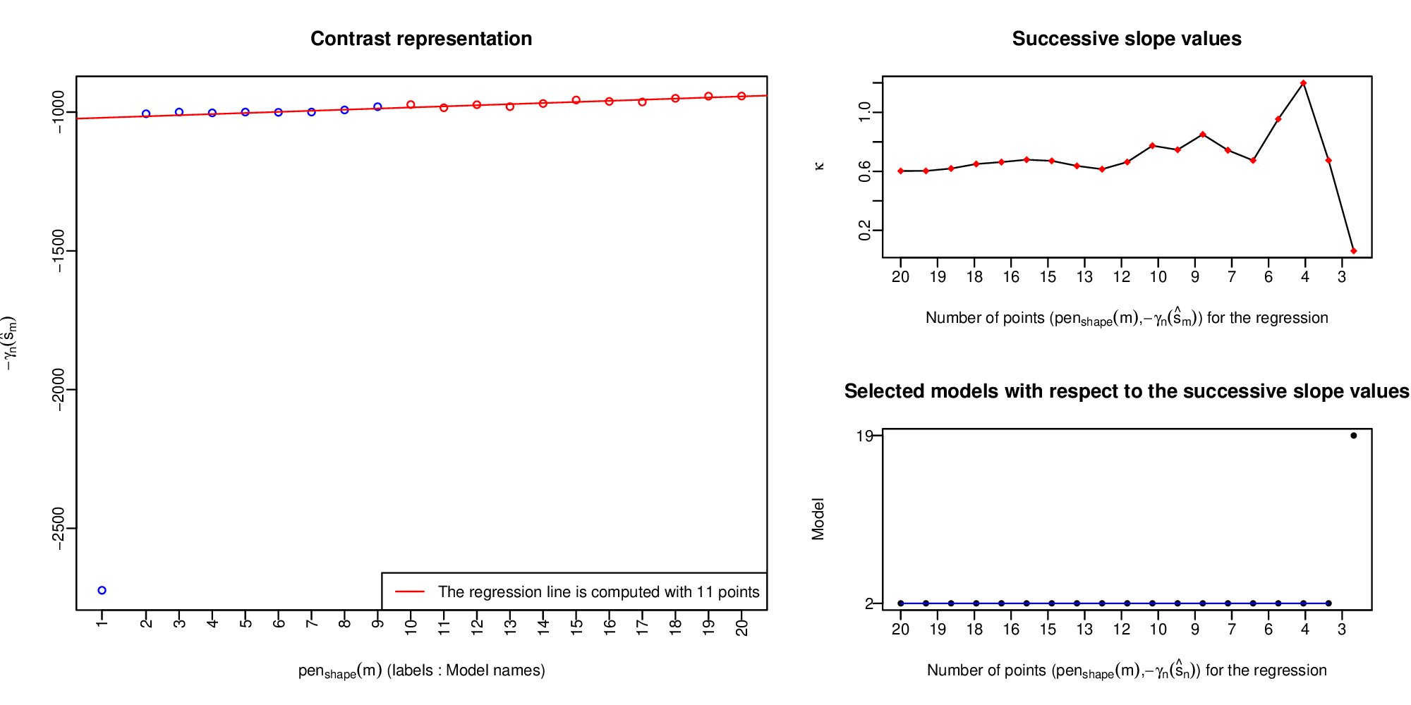
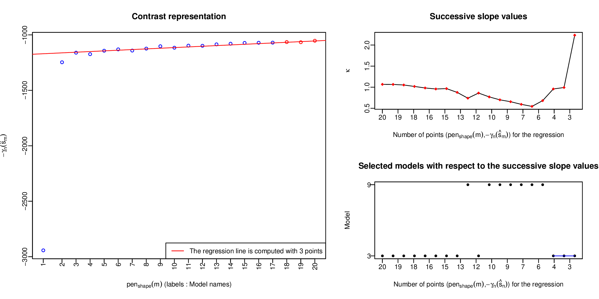
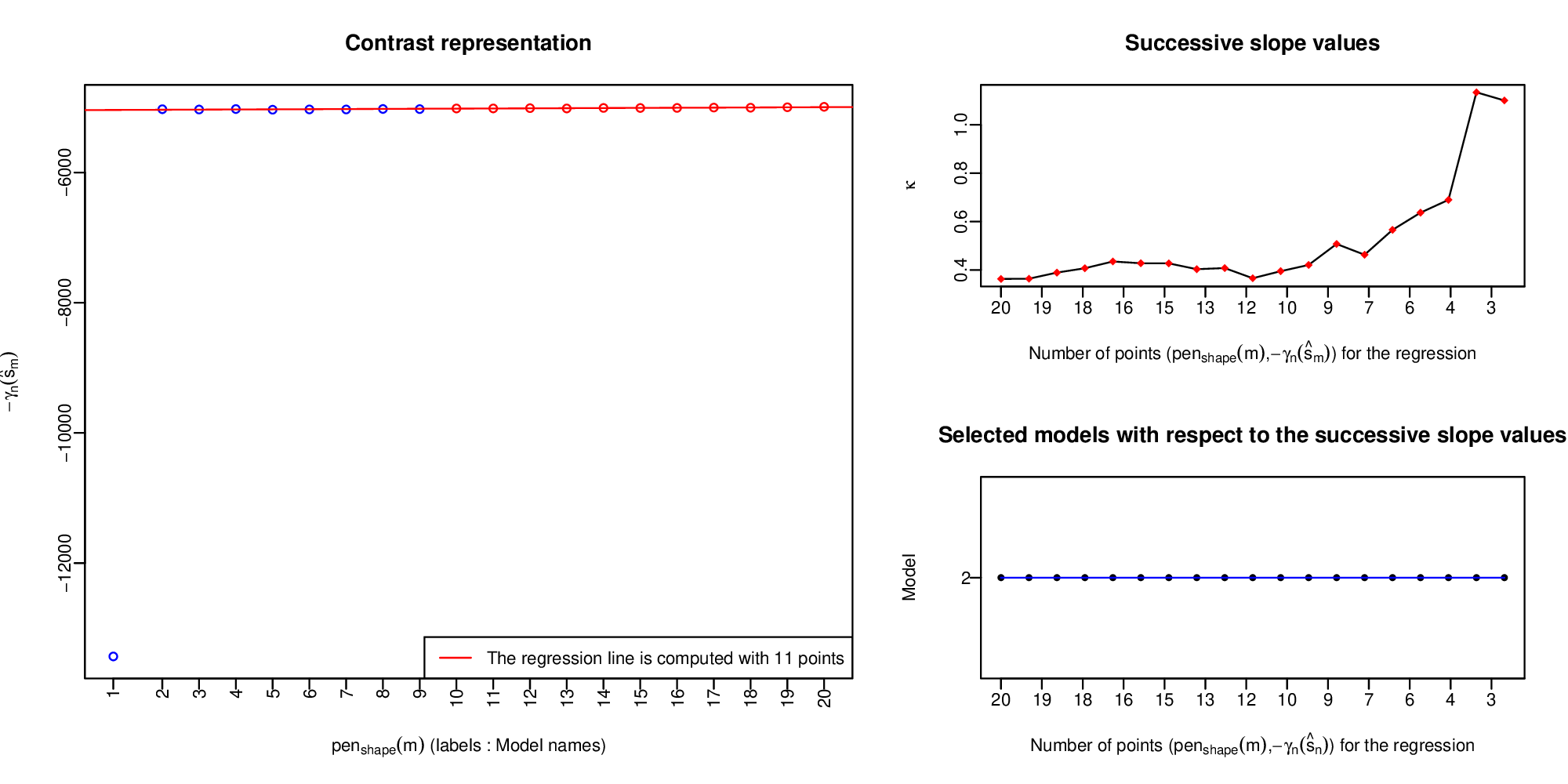
In our numerical experiment, namely, Figures 3 and 4, we confirm the validity of the linear penalty shape assumption, which supports the use of penalties proportional to the dimension. This implies that the logarithm terms are not detected in practice as shown in Figures 3 and 4 and thus only the preponderant term in $dim (S_{𝐦})$ is retained in the penalty form.

In particular, based on Appendix B.4 from Cohen and Le Pennec (2011), we can make explicit the dependence of the theoretical constant $κ$ , with respect to $ρ$ and $C_{1}$ as follows. For instance, in Theorem 3.3, given any $ρ \in (0, 1)$ and $C_{1} > 1$ , define $ϵ_{pen} = 1 - \frac{1}{C_{1}}$ . Then $κ$ is determined by

κ = \frac{κ^{'}_{0} (κ^{'}_{1} + κ^{'}_{2})^{2} (\sqrt{1 + \frac{72 C_{ρ} ϵ_{pen}}{ρ κ^{'}_{0} (κ^{'}_{1} + κ^{'}_{2})^{2}}} + 1)}{2 C_{ρ} ϵ_{pen}} + \frac{18}{ρ},

where $ϵ_{d}$ is a given positive constant and

	$κ^{'}_{0}$	$= \frac{2 (2 + ϵ_{d})}{1 + ϵ_{d}}, κ^{'}_{1} = \frac{1}{\sqrt{ρ (1 - ρ)}} (3 κ^{'}_{3} \sqrt{2} + 12 + 16 \sqrt{\frac{1 - ρ}{ρ}}),$
	$κ^{'}_{3}$	$\leq 27, κ^{'}_{2} = \frac{1}{\sqrt{ρ (1 - ρ)}} (42 + \frac{3}{4 \sqrt{κ^{'}_{0}}}) .$

For example, if $ρ = \frac{1}{2}$ , $C_{1} = 2$ , $ϵ_{d} = 1$ , $κ_{3}^{'} = 27$ , then $ϵ_{pen} = 1 - \frac{1}{C_{1}} = \frac{1}{2}$ , $κ_{0}^{'} = 3$ , $κ_{1}^{'} = 56 + 162 \sqrt{2}$ , $κ_{2}^{'} = 84 + \frac{\sqrt{3}}{2}$ , and

	$C_{ρ}$	$= \frac{1}{ρ} \min (\frac{1 - ρ}{ρ}, 1) (\ln (1 + \frac{ρ}{1 - ρ}) - ρ) = 2 \ln 2 - 1,$
	$κ$	$\approx 2126069 .$		(3.7)

According to the previous example, we can see that the theoretical penalty is lower bounded by $κ$ , which can be large in practice. This result is not surprising since, according to (Cohen and Le Pennec, 2011, Appendix B.4, page 40, line 7), if we choose $ϵ_{d}$ small enough then $κ$ scales proportionally to

\frac{1}{C_{ρ} ρ (1 - ρ) ϵ_{pen}} = \frac{ρ}{(1 - ρ)^{2} (\ln (1 + \frac{ρ}{1 - ρ}) - ρ)}

and thus explodes to $+ \infty$ when $ρ$ goes to $1$ and $C_{1}$ goes to $1$ . Therefore, it is important to study a natural question as to whether the constant $κ$ appearing in the penalty can be estimated from the data without losing theoretical guaranties on the performance? No definite answer exists so far for MoE regression models, however at least our numerical experiment in Section 5 shows that the slope heuristic proposed by Birgé and Massart (2007) may lead to a good practical solution. In particular, we seek to mathematically and fully justify the slope heuristic in MoE regression models as in least-squares regression on a random (or fixed) design with regressogram (projection) estimators, respectively, see Birgé and Massart (2007); Arlot and Massart (2009); Arlot and Bach (2009); Arlot (2019) for greater details. Furthermore, as is often the case in empirical processes theory, the constant $κ$ appearing in the bound is pessimistic as shown in (3.3). Numerical experiments in Section 5 show that there is a hope that this is only a technical issue. For instance, Figures 5 and 6 show that the practical values of $κ$ , selecting by slope heuristic, are generally very small compared to the theoretical values.

4 Proofs of finite-sample oracle inequalities and main mathematical challenges

4.1 Proof for deterministic collections of GLoME models

The deterministic collection of MoE models include GLLiM, GLoME, SGaME and LinBoSGaME models, where finite-sample oracle inequalities have only been well studied for the latter two models (Cohen and Le Pennec, 2011, Theorem 2), see also (Cohen and Le Pennec, 2013, Theorem 2.2.) and (Montuelle et al., 2014, Theorem 2). We first summarize this general model selection theorem and the techniques that Montuelle et al. (2014) used to control the bracketing entropy of LinBoSGaME models with softmax gating networks in Sections 4.1.1 and 4.1.2, respectively. Then, we explain why such techniques can not be directly applied to our collection of GLoME models via Section 4.1.3 and propose our approach to highlight the main issues and our contributions.

4.1.1 A general conditional density model selection theorem for deterministic collection of models

Before stating a general model selection theorem for conditional densities, we have to present some regularity assumptions.

First, we need an information theory type assumption to control the complexity of our collection. We assume the existence of a Kraft-type inequality for the collection (Massart, 2007; Barron et al., 2008).

Assumption 4.1 (K).

There is a family $(z_{𝐦})_{𝐦 \in ℳ}$ of non-negative numbers and a real number $Ξ$ such that

Ξ = \sum_{𝐦 \in ℳ} e^{- z_{𝐦}} < + \infty .

For technical reasons, a separability assumption, always satisfied in the setting of this paper, is also required. It is a mild condition, which is classical in empirical process theory (Van Der Vaart and Wellner, 1996; van de Geer, 2000). 4.2 allows us to work with a countable subset.

Assumption 4.2 (Sep).

For every model $S_{𝐦}$ in the collection $(S_{𝐦})_{𝐦 \in ℳ}$ , there exists some countable subset $S^{'}_{𝐦}$ of $S_{𝐦}$ and a set $𝒳^{'}_{𝐦}$ with $ι (𝒳 ∖ 𝒳^{'}_{𝐦}) = 0$ , where $ι$ denotes Lebesgue measure, such that for every $t \in S_{𝐦}$ , there exist some sequences $(t_{k})_{k \geq 1}$ of elements of $S^{'}_{𝐦}$ , such that for every $𝐲 \in 𝒴$ and every $𝐱 \in 𝒳^{'}_{𝐦}, \ln (t_{k} (𝐱 ∣ 𝐲)) \overset{k \to + \infty}{\to} \ln (t (𝐱 ∣ 𝐲))$ .

Next, recall that the bracketing entropy of a set $S$ with respect to any distance $d$ , denoted by $ℋ_{[\cdot], d} ((δ, S))$ , is defined as the logarithm of the minimal number $𝒩_{[\cdot], d} (δ, S)$ of brackets $[t^{-}, t^{+}]$ covering $S$ , such that $d (t^{-}, t^{+}) \leq δ$ . That is,

N_{[\cdot], d} (δ, S) : = \min {n \in ℕ^{⋆} : \exists [t^{-}_{k}, t^{+}_{k}]_{k \in [n]} s.t d (t^{-}_{k}, t^{+}_{k}) \leq δ, S \subset ⋃_{k = 1}^{n} [t^{-}_{k}, t^{+}_{k}]} .

(4.1)

Here, $s \in [t^{-}_{k}, t^{+}_{k}]$ means that $t^{-}_{k} (𝐱, 𝐲) \leq s (𝐱, 𝐲) \leq t^{+}_{k} (𝐱, 𝐲)$ , $\forall (𝐱, 𝐲) \in 𝒳 \times 𝒴$ .

We also need the following important 4.3 on Dudley-type integral of these bracketing entropies, which is often utilized in empirical process theory (Van Der Vaart and Wellner, 1996; van de Geer, 2000; Kosorok, 2007).

Assumption 4.3 (H).

For every model $S_{𝐦}$ in the collection $𝒮$ , there is a non-decreasing function $ϕ_{𝐦}$ such that $δ \mapsto \frac{1}{δ} ϕ_{𝐦} (δ)$ is non-increasing on $(0, \infty)$ and for every $δ \in ℝ^{+}$ ,

\int_{0}^{δ} \sqrt{ℋ_{[\cdot], d^{\otimes n}} (δ, S_{𝐦} (\tilde{s}, δ))} d δ \leq ϕ_{𝐦} (δ),

where $S_{𝐦} (\tilde{s}, δ) = {s_{𝐦} \in S_{𝐦} : d^{\otimes n} (\tilde{s}, s_{𝐦}) \leq δ}$ . The model complexity of $S_{𝐦}$ is then defined as $𝒟_{𝐦}$ = $n δ^{2}_{𝐦}$ , where $δ_{𝐦}$ is the unique root of $\frac{1}{δ} ϕ_{𝐦} (δ) = \sqrt{n} δ$ .

Observe that the model complexity does not depend on the bracketing entropies of the global models $S_{𝐦}$ , but rather on those of smaller localized sets $S_{𝐦} (\tilde{s}, δ)$ . We are now able to state an important weak oracle inequality, Theorem 4.5, originally from (Cohen and Le Pennec, 2011, 2013, Theorem 2).

Theorem 4.5.

Assume that we observe $(𝐱_{[n]}, 𝐲_{[n]})$ , arising from an unknown conditional density $s_{0}$ . Let $𝒮 = (S_{𝐦})_{𝐦 \in ℳ}$ be an at most countable conditional density model collection. Assume that 4.1 (K), 4.2 (Sep), and 4.3 (H) hold for every model $S_{𝐦} \in 𝒮$ . Then, for any $ρ \in (0, 1)$ and any $C_{1} > 1$ , there is a constant $κ$ depending only on $ρ$ and $C_{1}$ , such that for every index $𝐦 \in ℳ$ ,

pen (𝐦) \geq κ (n δ_{𝐦}^{2} + z_{𝐦})

with $δ_{𝐦}$ is the unique root of $\frac{1}{δ} ϕ_{𝐦} (δ) = \sqrt{n} δ$ , such that the $η^{'}$ -penalized likelihood estimator $\hat{s}_{\hat{𝐦}}$ satisfies

	$𝔼_{𝐗_{[n]}, 𝐘_{[n]}} [J K L_{ρ}^{\otimes n} (s_{0}, \hat{s}_{\hat{𝐦}})]$	$\leq C_{1} i n f_{𝐦 \in ℳ} (i n f_{s_{𝐦} \in S_{𝐦}} K L^{\otimes n} (s_{0}, s_{𝐦}) + \frac{pen (𝐦)}{n})$
		$+ \frac{κ C_{1} Ξ}{n} + \frac{η + η^{'}}{n} .$		(4.2)

For the sake of generality, Theorem 4.5 is relatively abstract. Since the assumptions of Theorem 4.5 are as general as possible. But from the practical point of view, a natural question is the existence of interesting model collections that satisfy these assumptions. We will sketch the proof for collection of LinBoSGaME models from (Montuelle et al., 2014, Theorem 1) and show that their result is not directly applicable to the GLoME setting. The main reason is that the technique for handling the linear combination of bounded functions for the weight functions of logistic schemes of Montuelle et al. (2014) is not valid for the Gaussian gating parameters in GLoME models. Therefore, we propose a reparameterization trick to bound the metric entropy of the Gaussian gating parameters space; see Section 4.1.3 for more details.

4.1.2 Sketch of the proof for LinBoSGaME models

To prove the main conditional density model selection theorem for LinBoSGaME models, (Montuelle et al., 2014, Theorem 1), the authors have to make use of Theorem 4.5. Then, they need to prove that their collection of LinBoSGaME models have to satisfy 4.1 (K), 4.2 (Sep), and 4.3 (H). However, they did not verify 4.1 (K) and 4.2 (Sep) and considered them as primative assumptions on their LinBoSGaME models because of the complexity of LinBoSGaME models and technical reasons. Therefore, the main difficulty remains on verifying 4.3 (H) via bracketing entropy controls of the linear combination of bounded functions for the weight functions of logistic schemes.

Firstly, they define the following distance over conditional densities:

sup_{𝐲} d_{𝐱} (s, t) = sup_{𝐲 \in 𝒴} (\int_{𝒳} (\sqrt{s (𝐱 ∣ 𝐲)} - \sqrt{t (𝐱 ∣ 𝐲)})^{2} d 𝐱)^{1 / 2} .

This leads straightforwardly to $d^{2 \otimes n} (s, t) \leq sup_{𝐲} d^{2}_{𝐱} (s, t)$ . Then, they also define

sup_{𝐲} d_{k} (g, g^{'}) = sup_{𝐲 \in 𝒴} (\sum_{k = 1}^{K} (\sqrt{g_{k} (𝐲)} - \sqrt{g^{'}_{k} (𝐲)})^{2})^{1 / 2},

for any gating functions $g$ and $g^{'}$ . To this end, given any densities $s$ and $t$ over $𝒳$ , the following distance, depending on $𝐲$ , is constructed as follows:

	$sup_{𝐲} \max_{k} d_{𝐱} (s, t)$	$= sup_{𝐲 \in 𝒴} \max_{k \in [K]} d_{𝐱} (s_{k} (\cdot, 𝐲), t_{k} (\cdot, 𝐲))$
		$= sup_{𝐲 \in 𝒴} \max_{k \in [K]} (\int_{𝒳} (\sqrt{s_{k} (𝐱, 𝐲)} - \sqrt{t_{k} (𝐱, 𝐲)})^{2} d 𝐱)^{1 / 2} .$

Then, they prove that definition of complexity of model $S_{𝐦}$ in 4.3 (H) is related to an classical entropy dimension with respect to a Hellinger type divergence $d^{\otimes n}$ , due to Proposition 4.6.

Proposition 4.6 (Proposition 2 from (Cohen and Le Pennec, 2011)).

For any $δ \in (0, \sqrt{2}]$ , such that $ℋ_{[\cdot], d^{\otimes n}} (δ, S_{𝐦}) \leq dim (S_{𝐦}) (C_{𝐦} + \ln (\frac{1}{δ}))$ , the function

ϕ_{𝐦} (δ) = δ \sqrt{dim (S_{𝐦})} (\sqrt{C_{𝐦}} + \sqrt{π} + \sqrt{\ln (\frac{1}{\min (δ, 1)})})

satisfies 4.3 (H). Furthermore, the unique solution $δ_{𝐦}$ of $\frac{1}{δ} ϕ_{𝐦} (δ) = \sqrt{n} δ$ , satisfies

n δ^{2}_{𝐦} \leq dim (S_{𝐦}) (2 (\sqrt{C_{𝐦}} + \sqrt{π})^{2} + (\ln \frac{n}{(\sqrt{C_{𝐦}} + \sqrt{π})^{2} dim (S_{𝐦})})_{+}) .

Therefore, Proposition 4.6 implies that 4.3 (H) can be proved via Lemma 4.7.

Lemma 4.7.

For any $δ \in (0, \sqrt{2}]$ , the collection of LinBoSGaME models, $𝒮 = (S_{𝐦})_{𝐦 \in ℳ}$ , satisfies

ℋ_{[\cdot], d^{\otimes n}} (δ, S_{𝐦}) \leq dim (S_{𝐦}) (C_{𝐦} + \ln (\frac{1}{δ})) .

Lemma 4.7 is then obtained by decomposing the entropy terms between the softmax gating functions and the Gaussian experts. Note that both LinBoSGaME and GLoME models share the same structures of Gaussian experts mean, see Figure 1 again for more details. Therefore, in Section 4.1.3, we only highlight our contributions regarding the control of bracketing entropy for the parameter of gating network compared to Montuelle et al. (2014).

More precisely, the authors of Montuelle et al. (2014) rewrite the softmax gating parameters’ space as follows:

	$𝐖_{K, d_{𝐖}}$	$= {0} \otimes 𝐖^{K - 1}, 𝐖 = {𝐲 \mapsto \sum_{d = 1}^{d_{𝐖}} ω_{d} θ_{𝐖, d} (𝐲) \in ℝ : \max_{d \in [d_{𝐖}]} \| ω_{d} \| \leq T_{𝐖}},$
	$𝒫_{K}$	$= {𝐲 \mapsto (\frac{e^{𝐰_{k} (𝐲)}}{\sum_{l = 1}^{K} e^{𝐰_{l} (𝐲)}})_{k \in [K]} = : (g_{𝐰, k} (𝐲))_{k \in [K]}, 𝐰 \in 𝐖_{K, d_{𝐖}}} .$

Then, they also require the definition of metric entropy of the set $𝒲_{K}$ : $ℋ_{d_{∥ sup ∥_{\infty}}} (δ, 𝒲_{K})$ , which measures the logarithm of the minimal number of balls of radius at most $δ$ , according to a distance $d_{∥ sup ∥_{\infty}}$ , needed to cover $𝒲_{K}$ where

d_{∥ sup ∥_{\infty}} ((s_{k})_{k \in [K]}, (t_{k})_{k \in [K]}) = \max_{k \in [K]} sup_{𝐲 \in 𝒴} ∥ s_{k} (𝐲) - t_{k} (𝐲) ∥_{2},

(4.3)

for any $K$ -tuples of functions $(s_{k})_{k \in [K]}$ , $(t_{k})_{k \in [K]}$ and $∥ s_{k} (𝐲) - t_{k} (𝐲) ∥_{2}$ is the Euclidean distance in $ℝ^{L}$ . By using Lemma 5 and Proposition 2 from (Montuelle et al., 2014), Lemma 4.7 holds true if we can prove Lemma 4.8. Note that the first inequality of Lemma 4.8 comes from (Montuelle et al., 2014, Lemma 4) and describes relationship between the bracketing entropy of $𝒫_{K}$ and the entropy of $𝒲_{K}$ .

Lemma 4.8.

For all $δ \in (0, \sqrt{2}]$ , there exists a constant $C_{𝒲_{K}}$ such that

	$ℋ_{[\cdot], sup_{𝐲} d_{k}} (\frac{δ}{5}, 𝒫_{K})$	$\leq ℋ_{d_{∥ sup ∥_{\infty}}} (\frac{3 \sqrt{3} δ}{20 \sqrt{K - 1}}, 𝒲_{K})$
		$\leq dim (𝒲_{K}) (C_{𝒲_{K}} + \ln (\frac{20 \sqrt{K - 1}}{3 \sqrt{3} δ})) .$

By the linearity from the construction of linear combination of a finite set of bounded functions whose coefficients belong to a compact set, in the argument from (Montuelle et al., 2014, Proof of Part 1 of Lemma 1, Page 1689), the second inequality of Lemma 4.8 is then easily established as follows.

Proof of the second inequality of Lemma 4.8.

Note that for all

𝐰 = (0, w_{k})_{k \in [K - 1]} \in 𝐖_{K, d_{𝐖}}, 𝐯 = (0, v_{k})_{k \in [K - 1]} \in 𝐖_{K, d_{𝐖}},

it holds that

	$d_{∥ sup ∥_{\infty}} (𝐰 - 𝐯)$	$= \max_{k \in [K - 1]} ∥ 𝒲_{K} - 𝐯_{k} ∥_{\infty}$
		$= \max_{k \in [K - 1]} sup_{𝐲 \in 𝐘} \| \sum_{i = 1}^{d_{𝐖}} ω_{k, i}^{𝐰} θ_{𝐖, i} (𝐲) - \sum_{i = 1}^{d_{𝐖}} ω_{k, i}^{𝐯} θ_{𝐖, i} (𝐲) \|$
		$\leq \max_{k \in [K - 1]} \sum_{i = 1}^{d_{𝐖}} \| ω_{k, i}^{𝐰} - ω_{k, i}^{𝐯} \| \underset{⏟}{sup_{𝐲 \in 𝐘} \| θ_{𝐖, i} (𝐲) \|}_{\leq 1}$
		$\leq d_{𝐖} \max_{k \in [K - 1], i \in [d_{𝐖}]} \| ω_{k, i}^{𝐰} - ω_{k, i}^{𝐯} \| .$

Therefore, we obtain

	$ℋ_{d_{∥ sup ∥_{\infty}}} (\frac{3 \sqrt{3} δ}{20 \sqrt{K - 1}}, 𝒲_{K})$
	$\leq ℋ_{d_{∥ sup ∥_{\infty}}} (\frac{3 \sqrt{3} δ}{20 \sqrt{K - 1} d_{𝐖}}, {𝝎 \in ℝ^{(K - 1) d_{𝐖}} : ∥ 𝝎 ∥_{\infty} \leq T_{𝐖}})$
	$\leq (K - 1) d_{𝐖} \ln (1 + \frac{20 \sqrt{K - 1} d_{𝐖} T_{𝐖}}{3 \sqrt{3} δ})$
	$\leq (K - 1) d_{𝐖} \ln (\sqrt{2} + \frac{20 \sqrt{K - 1} d_{𝐖} T_{𝐖}}{3 \sqrt{3}} + \ln (\frac{1}{δ})) .$

∎

However, proving Lemma 4.9, our equivalent of Lemma 4.8, will be much harder and could be used for controlling the bracketing entropy for many standard MoE regression models with Gaussian gating networks, see Section 4.1.3 for more details.

4.1.3 Our contributions on the proof for GLoME models

To prove Theorem 3.3, we also need to make use of Theorem 4.5. Then, our model collection has to satisfy 4.1 (K), 4.2 (Sep), and 4.3 (H).

Note that in the proof of LinBoSGaME models, the authors of Montuelle et al. (2014) did not prove 4.1 (K) and 4.2 (Sep) and considered them as assumptions on their LinBoSGaME models because of the complexity of LinBoSGaME models and technical reasons. However, in our proof for GLoME models, we consider an explicit example where the model is defined by $ℳ = 𝒦 \times 𝒟_{𝚼} = [K_{\max}] \times [d_{\max}]$ , $K_{\max}, d_{\max} \in ℕ^{⋆}$ , leads to the 4.1 (K) is always satisfied. It is interesting to find the optimal family $(z_{𝐦})_{𝐦 \in ℳ}$ satisfying 4.1 (K). To the best of our knowledge, this question is only partially answered in some special cases of MoE regression models, e.g., Gaussian graphical model Devijver and Gallopin (2018), Gaussian finite mixture models Maugis and Michel (2011a), finite mixture of Gaussian regression models Devijver (2015b, 2017b). However, for the standard MoE regression models such as LinBoSGaME and GLoME models, such question still remains open due to the complexity of models. We hope to resolve this important and interesting problem in our future work. Furthermore, note that the 4.2 (Sep) is true when we consider Gaussian densities Massart (2007).

Therefore, our model has only to satisfy the remaining 4.3 (H). Following the same strategy as in the proof of LinBoSGaME models, the main task for GLoME models is to establish Lemma 4.9, which is much more difficult compared to Lemma 4.8 and is proved in Section A.2.

For the Gaussian gating parameters, to make use of the first inequality from Lemma 4.8 of Montuelle et al. (2014), we propose the following reparameterization trick of the Gaussian gating space, which is defined in (2.2), via the logistics scheme $𝒫_{K}$ and the nonlinear space $𝒲_{K}$ as follows:

	$𝒲_{K}$	$= {𝐲 \mapsto (\ln (π_{k} ϕ_{L} (𝐲; 𝐜_{k}, 𝚪_{k})))_{k \in [K]} = : (𝐰_{k} (𝐲; 𝝎))_{k \in [K]} = 𝐰 (𝐲; 𝝎) : 𝝎 \in \tilde{𝛀}_{K}},$
	$𝒫_{K}$	$= {𝐲 \mapsto (\frac{e^{𝐰_{k} (𝐲)}}{\sum_{l = 1}^{K} e^{𝐰_{l} (𝐲)}})_{k \in [K]} = : (g_{𝐰, k} (𝐲))_{k \in [K]}, 𝐰 \in 𝒲_{K}} .$		(4.4)

We aim to provide the following important upper bound for metric entropy of nonlinear space Lemma 4.9, which play a key step for controlling the bracketing entropy not only for GLoME models but also for any standard MoE regression models with Gaussian gating networks, e.g., BLLiM and BLoME models, see again Figure 1 for comprehensive descriptions of this general class.

Lemma 4.9.

For all $δ \in (0, \sqrt{2}]$ , there exists a constant $C_{𝒲_{K}}$ such that

	$ℋ_{[\cdot], sup_{𝐲} d_{k}} (\frac{δ}{5}, 𝒫_{K})$	$\leq ℋ_{d_{∥ sup ∥_{\infty}}} (\frac{3 \sqrt{3} δ}{20 \sqrt{K - 1}}, 𝒲_{K})$
		$\leq dim (𝒲_{K}) (C_{𝒲_{K}} + \ln (\frac{20 \sqrt{K - 1}}{3 \sqrt{3} δ})) .$

More precisely, 4.3 (H) is proved due to Lemma 4.7 and the following Lemma 4.10 by using the fact that $\sum_{k = 1}^{K} g_{𝐰, k} (𝐲) = 1, \forall 𝐲 \in 𝒴, \forall 𝐰 \in 𝒲_{K}$ and $ℋ_{[\cdot], d^{\otimes n}} (δ, S_{𝐦}) \leq ℋ_{[\cdot], sup_{𝐲} d_{𝐱}} (δ, S_{𝐦})$ , which is obtained by definition of bracketing entropy and $d^{\otimes n} (s, t) \leq sup_{𝐲} d_{𝐱} (s, t)$ .

Lemma 4.10 (Lemma 5 from Montuelle et al. (2014)).

Let

𝒢_{K, d}

= {𝒳 \times 𝒴 ∋ (𝐱, 𝐲) \mapsto (Φ_{D} (𝐱; 𝒗_{k, d} (𝐲), 𝚺_{k}))_{k \in [K]} : 𝝊_{d} \in 𝚼_{K, d}, 𝚺 \in 𝐕_{K}} .

For all $δ \in (0, \sqrt{2}]$ and $𝐦 \in ℳ$ ,

ℋ_{[\cdot], sup_{𝐲} d_{𝐱}} (δ, S_{𝐦}) \leq ℋ_{[\cdot], sup_{𝐲} d_{k}} (\frac{δ}{5}, 𝒫_{K}) + ℋ_{[\cdot], sup_{𝐲} \max_{k} d_{𝐱}} (\frac{δ}{5}, 𝒢_{K, d}) .

By making use of Lemma 4.10, the remaining task is to control the bracketing entropy of the Gaussian gating functions and experts separately via Lemmas 4.9 and 4.11, which are proved in Sections A.2 and A.3, respectively.

Lemma 4.11.

For all $δ \in (0, \sqrt{2}]$ , there exists a constant $C_{𝒢_{K, d}}$ such that

ℋ_{[\cdot], sup_{𝐲} \max_{k} d_{𝐱}} (\frac{δ}{5}, 𝒢_{K, d}) \leq dim (𝒢_{K, d}) (C_{𝒢_{K, d}} + \ln (\frac{1}{δ})) .

(4.5)

To this end, Lemma 4.10 allows us to conclude that given $ℭ = C_{𝒲_{K}} + \ln (\frac{5 K_{\max} \sqrt{K_{\max}}}{a_{W}}) + C_{𝒢_{K, d}}$ ,

	$ℋ_{[\cdot], sup_{𝐲} d_{𝐱}} (δ, S_{𝐦})$	$\leq ℋ_{[\cdot], sup_{𝐲} d_{k}} (\frac{δ}{5}, 𝒫_{K}) + ℋ_{[\cdot], sup_{𝐲} \max_{k} d_{𝐱}} (\frac{δ}{5}, 𝒢_{K, d})$
		$\leq dim (S_{𝐦}) (ℭ + \ln (\frac{1}{δ})) .$

Then, Proposition 4.6 leads to

n δ^{2}_{𝐦} \leq dim (S_{𝐦}) (2 (\sqrt{ℭ} + \sqrt{π})^{2} + (\ln \frac{n}{(\sqrt{ℭ} + \sqrt{π})^{2} dim (S_{𝐦})})_{+}) .

Finally, Theorem 4.5 implies that for any given collection of GLoME models $(S_{𝐦})_{𝐦 \in ℳ}$ , the oracle inequality of Theorem 3.3 is satisfied if $pen (𝐦)$ is bounded from below by

κ (dim (S_{𝐦}) (2 (\sqrt{ℭ} + \sqrt{π})^{2} + (\ln \frac{n}{(\sqrt{ℭ} + \sqrt{π})^{2} dim (S_{𝐦})})_{+}) + z_{𝐦}) .

4.2 Proof of random subcollection of BLoME models

The random subcollection of MoE models include BLLiM and BLoME models where finite-sample oracle inequalities were only well studied for finite mixture of Gaussian regression models via a model selection theorem for MLE among a random subcollection of models in regression framework of (Devijver, 2015b, Theorem 5.1), see also (Devijver and Gallopin, 2018, Theorem 7.3). This is an extension of a whole collection of conditional densities from (Cohen and Le Pennec, 2011, Theorem 2), and of (Massart, 2007, Theorem 7.11), working only for density estimation. In Section 4.2.1, we first summarize this theorem and the techniques that Devijver (2017b) used to control the bracketing entropy of finite mixture of Gaussian regression models with joint rank and variable selection for parsimonious estimation in a high-dimensional framework. Then, we explain why such techniques can not be applied to our collection of BLLiM and BLoME models to highlight the main challenges and our contributions.

4.2.1 A model selection theorem for MLE among a random subcollection

We can now state the main result of (Devijver, 2015b, Theorem 5.1) for the model selection theorem for MLE among a random subcollection.

Theorem 4.12 (Theorem 5.1 from Devijver (2015b)).

Let $(𝐱_{[n]}, 𝐲_{[n]})$ be observations coming from an unknown conditional density $s_{0}$ . Let the model collection $(S_{𝐦})_{𝐦 \in ℳ}$ be an at most countable collection of conditional density sets. Assume that 4.1 (K), 4.2 (Sep), and 4.3 (H) hold for every $𝐦 \in ℳ$ . Let $ϵ_{K L} > 0$ , and $\bar{s}_{𝐦} \in S_{𝐦}$ , such that

K L^{\otimes n} (s_{0}, \bar{s}_{𝐦}) \leq i n f_{t \in S_{𝐦}} K L^{\otimes n} (s_{0}, t) + \frac{ϵ_{K L}}{n};

and let $τ > 0$ , such that

\bar{s}_{𝐦} \geq e^{- τ} s_{0} .

(4.6)

Introduce $(S_{𝐦})_{𝐦 \in \tilde{ℳ}}$ , a random subcollection of $(S_{𝐦})_{𝐦 \in ℳ}$ . Consider the collection $(\hat{s}_{𝐦})_{𝐦 \in \tilde{ℳ}}$ of $η$ -log likelihood minimizer satisfying (2.26) for all $𝐦 \in \tilde{ℳ}$ . Then, for any $ρ \in (0, 1)$ , and any $C_{1} > 1$ , there are two constants $κ$ and $C_{2}$ depending only on $ρ$ and $C_{1}$ , such that, for every index $𝐦 \in ℳ$ ,

pen (𝐦) \geq κ (𝒟_{𝐦} + (1 \lor τ) z_{𝐦}),

and where the model complexity $𝒟_{𝐦}$ is defined in 4.3 (H), the $η^{'}$ -penalized likelihood estimator $\hat{s}_{\hat{𝐦}}$ , defined as in (2.27) on the subset $\tilde{ℳ} \subset ℳ$ , satisfies

	$𝔼_{𝐗_{[n]}, 𝐘_{[n]}} [J K L_{ρ}^{\otimes n} (s_{0}, \hat{s}_{\hat{𝐦}})]$	$\leq C_{1} 𝔼_{𝐗_{[n]}, 𝐘_{[n]}} [i n f_{𝐦 \in \tilde{ℳ}} (i n f_{t \in S_{𝐦}} K L^{\otimes n} (s_{0}, t) + 2 \frac{pen (𝐦)}{n})]$
		$+ C_{2} (1 \lor τ) \frac{Ξ^{2}}{n} + \frac{η^{'} + η}{n} .$

4.2.2 Sketch of the proof for BLoME models

To work with conditional density estimation in the BLLiM and BLoME models, it is natural to make use of Theorem 4.5. However, it is worth mentioning that because the model collection constructed by the BLLiM Devijver et al. (2017) or by some suitable procedures for BLoME models in practice is usually random, we have to use a model selection theorem for MLE among a random subcollection (cf. (Devijver, 2015b, Theorem 5.1) and (Devijver and Gallopin, 2018, Theorem 7.3)).

More precisely, we explain how Theorem 4.12 implies the finite-sample oracle inequality, Theorem 3.4. To this end, our collections of BLoME models has to satisfy some regularity assumptions, see Section 4.2.3 for more details. For BLoME models, the main difficulty in proving our oracle inequality lies in bounding the bracketing entropy of the Gaussian gating functions and Gaussian experts with block-diagonal covariance matrices. To overcome the former issue, we follow a reparameterization trick of the Gaussian gating parameters space in (4.1.3) and Lemma 4.9. For the second one, based on some ideas of Gaussian mixture models from Genovese and Wasserman (2000); Maugis and Michel (2011a), we contribute a novel extension for standard MoE models with Gaussian gating networks. Note that our contributions extend the recent novel result on block-diagonal covariance matrices in Devijver and Gallopin (2018), which is only developed for Gaussian graphical models.

4.2.3 Our contributions on BLoME models

It should be stressed that all we need is to verify that 4.3 (H), 4.2 (Sep) and 4.1 (K) hold for every $𝐦 \in ℳ$ . According to the result from (Devijver, 2015b, Section 5.3), 4.2 (Sep) holds when we consider Gaussian densities and the assumption defined by (4.6) is true if we assume further that the true conditional density $s_{0}$ is bounded and compactly supported. Furthermore, since we restricted $d$ and $K$ to $𝒟_{𝚼} = [d_{\max}]$ and $𝒦 = [K_{\max}]$ , respectively, it is true that there exists a family $(z_{𝐦})_{𝐦 \in ℳ}$ and $Ξ > 0$ such that, 4.1 (K) is satisfied. Therefore, the proof for the remaining 4.3 (H) is our novel contribution. In particular, to the best of our knowledge, there are no results that can be directly applied to 4.3 (H) for BLoME models due to their complexity with the Gaussian gating functions and Gaussian experts with block-diagonal covariance matrices. This highlights our contributions to this challenging problem concerning the work of Genovese and Wasserman (2000); Maugis and Michel (2011a); Devijver (2015b, 2017b); Devijver and Gallopin (2018); Montuelle et al. (2014).

By using Lemma 4.7, 4.3 (H) holds true if we can prove that for any $δ \in (0, \sqrt{2}]$ , the collection of LinBoSGaME models, $𝒮 = (S_{𝐦})_{𝐦 \in ℳ}$ , satisfies

ℋ_{[\cdot], d^{\otimes n}} (δ, S_{𝐦}) \leq dim (S_{𝐦}) (C_{𝐦} + \ln (\frac{1}{δ})) .

(4.7)

Proof of 4.7.

Note that (4.7) can be established by first decomposing the entropy term between the Gaussian gating functions and the Gaussian experts. Motivated by our reparameterization trick of the Gaussian gating space in Section 4.1.3 and (4.1.3), we define Gaussian experts $𝒢_{K, d, 𝐁}$ as follows.

𝒢_{K, d, 𝐁}

= {(𝐱, 𝐲) \mapsto (ϕ (𝐱; 𝝊_{k, d} (𝐲), 𝚺_{k} (𝐁_{k})))_{k \in [K]} : 𝝊_{d} \in 𝚼_{K, d}, 𝚺 (𝐁) \in 𝐕_{K} (𝐁)} .

There are two possible ways to decompose the bracketing entropy of $S_{𝐦}$ based on different distances. For the first approach, we can use Lemma 4.13 (Montuelle et al., 2014, Lemma 5):

Lemma 4.13.

For all $δ \in (0, \sqrt{2}]$ and $𝐦 \in ℳ$ ,

ℋ_{[\cdot], sup_{𝐲} d_{𝐱}} (δ, S_{𝐦}) \leq ℋ_{[\cdot], sup_{𝐲} d_{k}} (\frac{δ}{5}, 𝒫_{K}) + ℋ_{[\cdot], sup_{𝐲} \max_{k} d_{𝐱}} (\frac{δ}{5}, 𝒢_{K, d, 𝐁}) .

As mentioning in Appendix B.2.1 from Montuelle et al. (2014), Lemma 4.13 boils down to assuming that $𝐘$ is bounded. Furthermore, they also claim that this boundedness assumption can be relaxed when using smaller distance $d^{\otimes n}$ but bounding the corresponding bracketing entropy becomes much more challenging. We successfully weaken such boundedness assumption via utilizing the smaller distance: $d^{\otimes n}$ , for the bracketing entropy of $S_{𝐦}$ although bounding such bracketing entropy for $𝒲_{K}$ and $𝒢_{K, ℬ}$ becomes much more challenging. This reinforces our new contributions concerning the control of bracketing entropy of BLoME models. Consequently, this leads to the second approach via Lemma 4.14 (Montuelle et al., 2014, Lemma 6).

Lemma 4.14.

For all $δ \in (0, \sqrt{2}]$ ,

ℋ_{[\cdot], d^{\otimes n}} (δ, S_{𝐦}) \leq ℋ_{[\cdot], d_{𝒫_{K}}} (\frac{δ}{2}, 𝒫_{K}) + ℋ_{[\cdot], d_{𝒢_{K, d, 𝐁}}} (\frac{δ}{2}, 𝒢_{K, d, 𝐁}),

where

	$d^{2}_{𝒫_{K}} (g^{+}, g^{-})$	$= 𝔼_{𝐘_{[n]}} [\frac{1}{n} \sum_{i = 1}^{n} d^{2}_{k} (g^{+} (𝐘_{i}), g^{-} (𝐘_{i}))]$
		$= 𝔼_{𝐘_{[n]}} [\frac{1}{n} \sum_{i = 1}^{n} \sum_{k = 1}^{K} (\sqrt{g^{+}_{k} (𝐘_{i})} - \sqrt{g^{-}_{k} (𝐘_{i})})^{2}],$
	$d^{2}_{𝒢_{K, d, 𝐁}} (ϕ^{+}, ϕ^{-})$	$= 𝔼_{𝐘_{[n]}} [\frac{1}{n} \sum_{i = 1}^{n} \sum_{k = 1}^{K} d^{2}_{𝐱} (ϕ^{+}_{k} (\cdot, 𝐘_{i}), ϕ^{-}_{k} (\cdot, 𝐘_{i}))]$
		$= 𝔼_{𝐘_{[n]}} [\frac{1}{n} \sum_{i = 1}^{n} \sum_{k = 1}^{K} \int_{𝒳} (\sqrt{ϕ^{+}_{k} (𝐱, 𝐘_{i})} - \sqrt{ϕ^{+}_{k} (𝐱, 𝐘_{i})})^{2} d 𝐱] .$

Next, we make use of Lemma 4.15, which is proved in Section A.4, to provide an upper bound on the bracketing entropy of $S_{𝐦}$ and $𝒫_{K}$ on the corresponding distances $d^{\otimes n}$ and $d_{𝒫_{K}}$ , respectively.

Lemma 4.15.

It holds that

	$d^{\otimes n} (s, t)$	$\leq sup_{𝐲} d_{𝐱} (s, t), and ℋ_{[\cdot], d^{\otimes n}} (δ, S_{𝐦}) \leq ℋ_{[\cdot], sup_{𝐲} d_{𝐱}} (δ, S_{𝐦}),$		(4.8)
	$d_{𝒫_{K}} (g^{+}, g^{-})$	$\leq sup_{𝐲} d_{k} (g^{+}, g^{-}), and ℋ_{[\cdot], d_{𝒫_{K}}} (\frac{δ}{2}, 𝒫_{K}) \leq ℋ_{[\cdot], sup_{𝐲} d_{k}} (\frac{δ}{2}, 𝒫_{K}) .$		(4.9)

Lemmas 4.14 and 4.15 imply that

ℋ_{[\cdot], d^{\otimes n}} (δ, S_{𝐦}) \leq ℋ_{[\cdot], sup_{𝐲} d_{k}} (\frac{δ}{2}, 𝒫_{K}) + ℋ_{[\cdot], d_{𝒢_{K, d, 𝐁}}} (\frac{δ}{2}, 𝒢_{K, d, 𝐁}) .

Based on this metric, one can first relate the bracketing entropy of $𝒫_{K}$ to $ℋ_{d_{∥ sup ∥_{\infty}}} (δ, 𝒲_{K})$ , and then obtain the upper bound for its entropy via Lemma 4.9. Then, we present our main contribution for BLoME models via Lemma 4.16. This lemma allows us to construct the Gaussian brackets to handle the metric entropy for Gaussian experts, which is established in Section A.5.

Lemma 4.16.

ℋ_{[\cdot], d_{𝒢_{K, d, 𝐁}}} (\frac{δ}{2}, 𝒢_{K, d, 𝐁}) \leq dim (𝒢_{K, d, 𝐁}) (C_{𝒢_{K, d, 𝐁}} + \ln (\frac{1}{δ})) .

(4.10)

Finally, (4.7) can easily proved via Lemmas 4.9 and 4.16. ∎

5 Numerical experiments

Note that our numerical experiments in Section 5, and the codes written in the R programming language (R Core Team, 2020) are available in the following link:
https://github.com/Trung-TinNGUYEN/NamsGLoME-Simulation.

5.1 The procedure

We illustrate our theoretical results in settings similar to those considered by Chamroukhi et al. (2010) and Montuelle et al. (2014), including simulated as well as real data sets. We first observe $n$ random samples $(𝐱_{i}, 𝐲_{i})_{i \in [n]}$ from an forward conditional density $s^{*}_{0}$ , and look for the best estimate among $s^{*}_{𝐦} \in S^{*}_{𝐦}, 𝐦 \in ℳ$ , defined in (2.2). We considered the simple case where the mean experts are linear functions, which leads to GLoME and supervised GLLiM are identical models. Our aim is to estimate the best number of components $K$ , as well as the model parameters. As described in more detail in Deleforge et al. (2015a), we use a GLLiM-EM algorithm to estimate the model parameters for each $K$ , and select the optimal model using the penalized approach that was described earlier. More precisely, in the following numerical experiments, the GLoME model is learned using functions from the package xLLiM, available on CRAN. It solves the inverse regression problem, defined in (2.18), and obtain the inverse maximum likelihood estimates (MLE) $(\hat{s}_{𝐦} (𝐱_{i} ∣ 𝐲_{i}))_{i \in [N]}$ , $𝐦 \in ℳ$ , then via (2.19), we obtain the forward MLE $(\hat{s}_{𝐦}^{*} (𝐲_{i} ∣ 𝐱_{i}))_{i \in [N]}$ , $𝐦 \in ℳ$ .

According to the general procedure for model selection, we first compute the forward MLE for each model $𝐦 \in ℳ$ , where $ℳ = 𝒦$ . Then, we select the model that satisfies the definition (2.27) with $pen (𝐦) = κ dim (S_{𝐦}^{*})$ , where $κ$ is a positive hyperparameter. The point we want to stress here is that the theoretical result stated in Theorem 3.3 gives the general form of penalty functions but it does not provide explicit penalties since the lower bounds on penalty functions in (3.1) are defined up to an unknown multiplicative constant $κ$ and mixture parameters are not bounded in practice. Nevertheless, Theorem 3.3 is required to justify the shape of penalties using for the slope heuristic and allows the number of variables $D$ as well as responses $L$ to be large compared to the fixed sample size $n$ . In particular, our Theorem 3.3 and Remark 2.2 guarantee that there exists a $κ$ large enough for which the estimate has the desired properties. Therefore, we need a data-driven method to choose $κ$ . According to the AIC or the BIC, we can select $κ = 1$ or $κ = \frac{\ln n}{2}$ . An important limitation of these criteria, however, is that they are only valid asymptotically. This implies that there are no finite-sample guarantees when using AIC or BIC for choosing between different levels of complexity. Their use in small sample settings is thus ad hoc. To overcome such difficulties, Birgé and Massart Birgé and Massart (2007) proposed a novel approach, called slope heuristics, supported by a non-asymptotic oracle inequality. This method leads to an optimal data-driven choice of multiplicative constants for penalties, e.g., $κ$ in our framework. Thus, we shall concentrate our attention on the slope heuristic for choosing the number of mixture components in our numerical experiments.

5.2 Simulated data sets

Note that our main objective here is to investigate how well the empirical tensorized Kullback–Leibler divergence between the true model ( $s_{0}^{*}$ ) and the selected model $\hat{s}_{\hat{𝐦}}^{*}$ follows the finite-sample oracle inequality of Theorem 3.3, as well as the rate of convergence of the error term. Therefore, we focus on $1$ -dimensional data sets, that is, with $L = D = 1$ . Beyond the statistical estimation and model selection objectives considered here, the dimensionality reduction capability of GLLiM in high-dimensional regression data, typically $D ≫ L$ , can be found in (Deleforge et al., 2015a, Section 6).

We construct simulated data sets following two scenarios: a well-specified (WS) case in which the true forward conditional density belongs to the class of proposed models:

	$s_{0}^{*} (y ∣ x)$	$= \frac{Φ (x; 0.2, 0.1)}{Φ (x; 0.2, 0.1) + Φ (x; 0.8, 0.15)} Φ (y; - 5 x + 2, 0.09)$
		$+ \frac{Φ (x; 0.8, 0.15)}{Φ (x; 0.2, 0.1) + Φ (x; 0.8, 0.15)} Φ (y; 0.1 x, 0.09),$

and a misspecified (MS) case, whereupon such an assumption is not true:

	$s_{0}^{*} (y ∣ x)$	$= \frac{Φ (x; 0.2, 0.1)}{Φ (x; 0.2, 0.1) + Φ (x; 0.8, 0.15)} Φ (y; x^{2} - 6 x + 1, 0.09)$
		$+ \frac{Φ (x; 0.8, 0.15)}{Φ (x; 0.2, 0.1) + Φ (x; 0.8, 0.15)} Φ (y; - 0.4 x^{2}, 0.09) .$

Figures 2(a) and 2(e) show some typical realizations of 2000 data points arising from the WS and MS scenarios. Note that by using GLoME, our estimator performs well in the WS setting (Figures 2(b) to 2(d)). In the MS case, we expect our algorithm to automatically balance the model bias and its variance (Figures 2(f) to 2(h)), which leads to the choice of a complex model, with $4$ mixture components. This observation will be elaborated upon in the subsequent experiments.

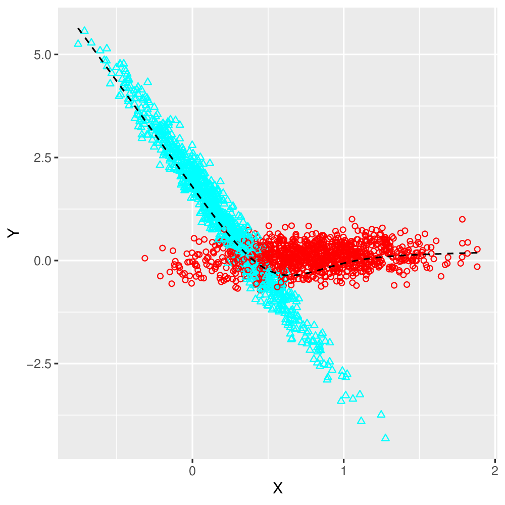
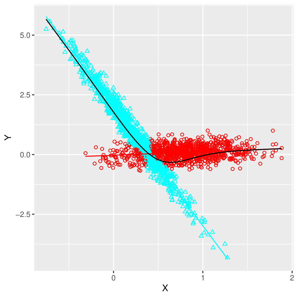
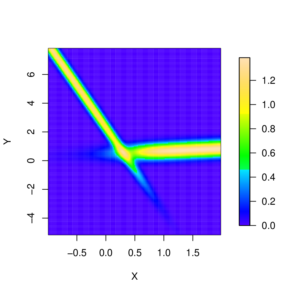
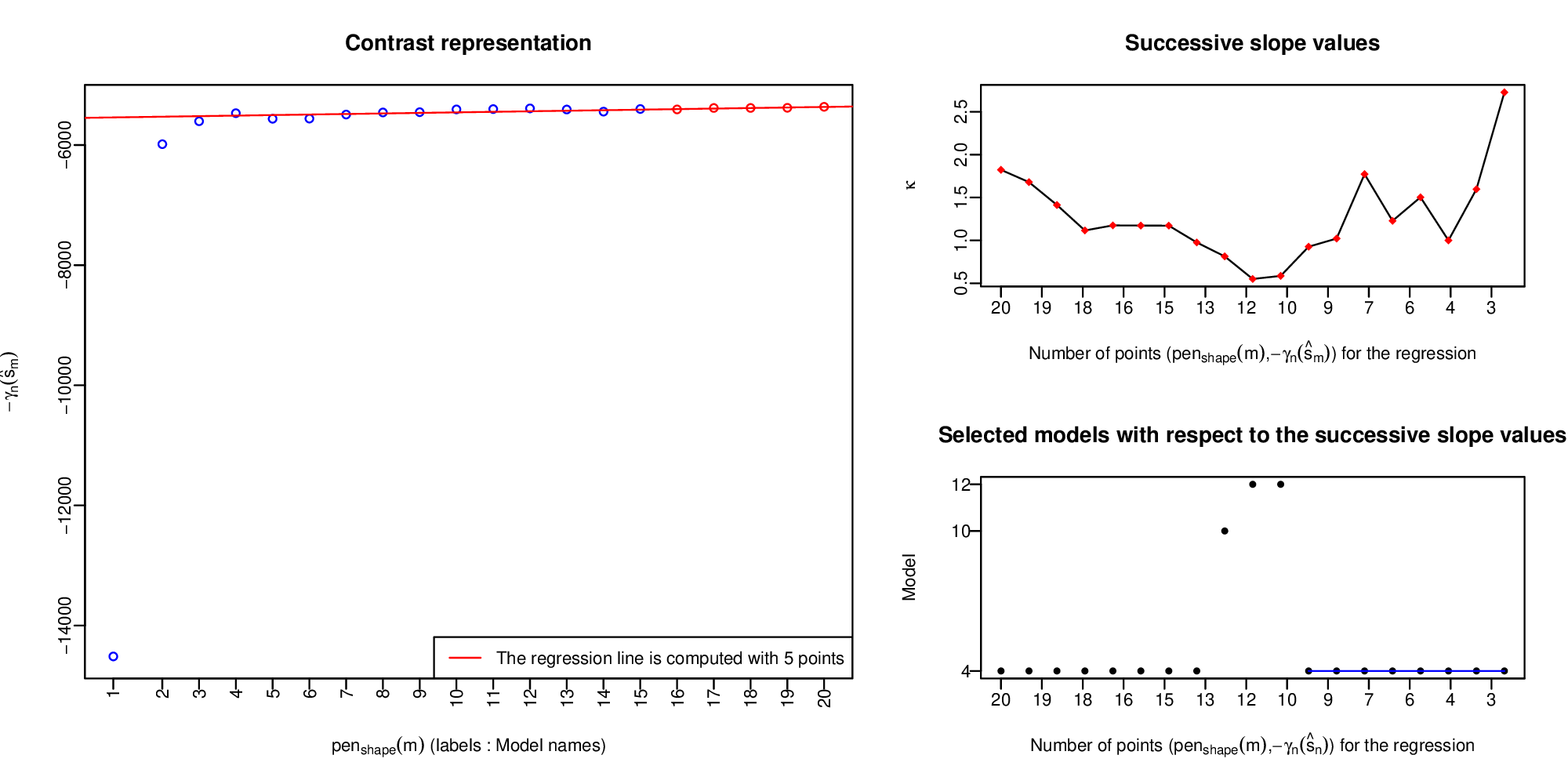
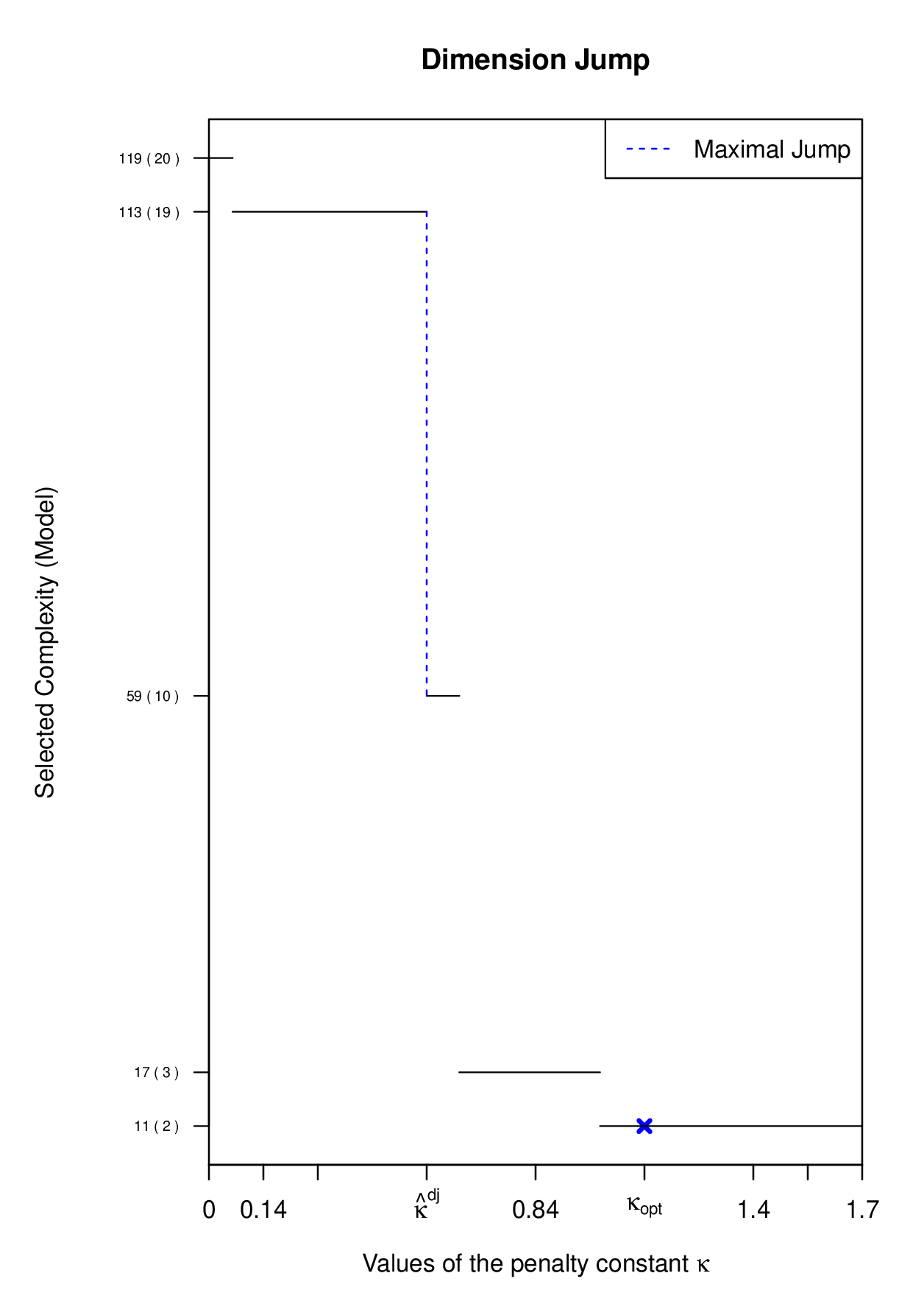
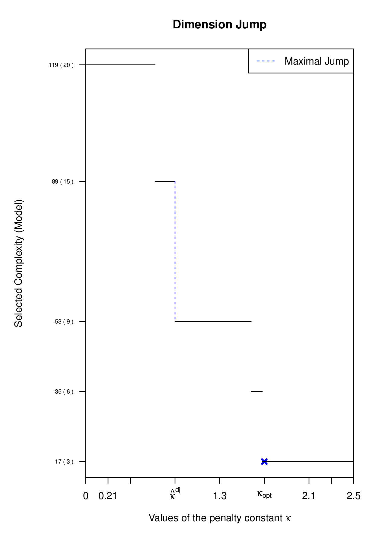
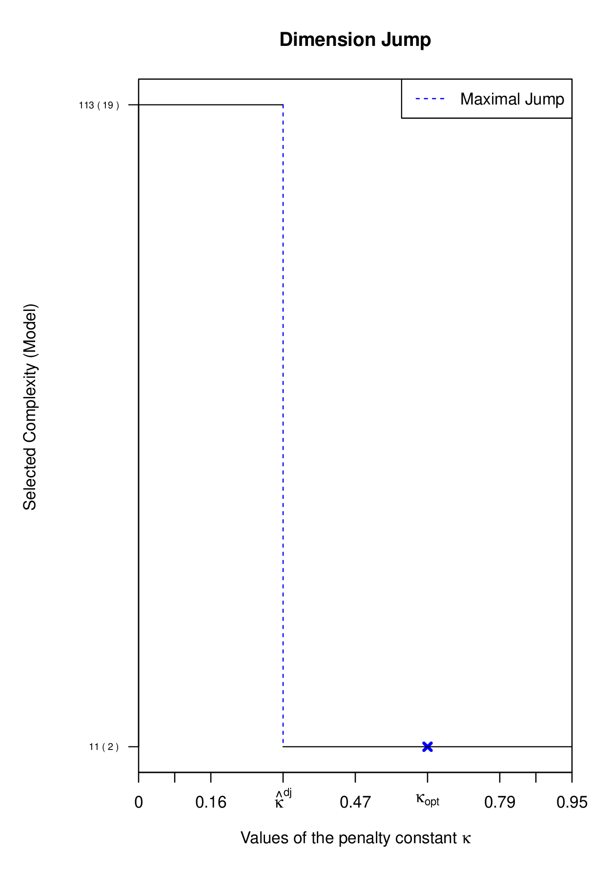
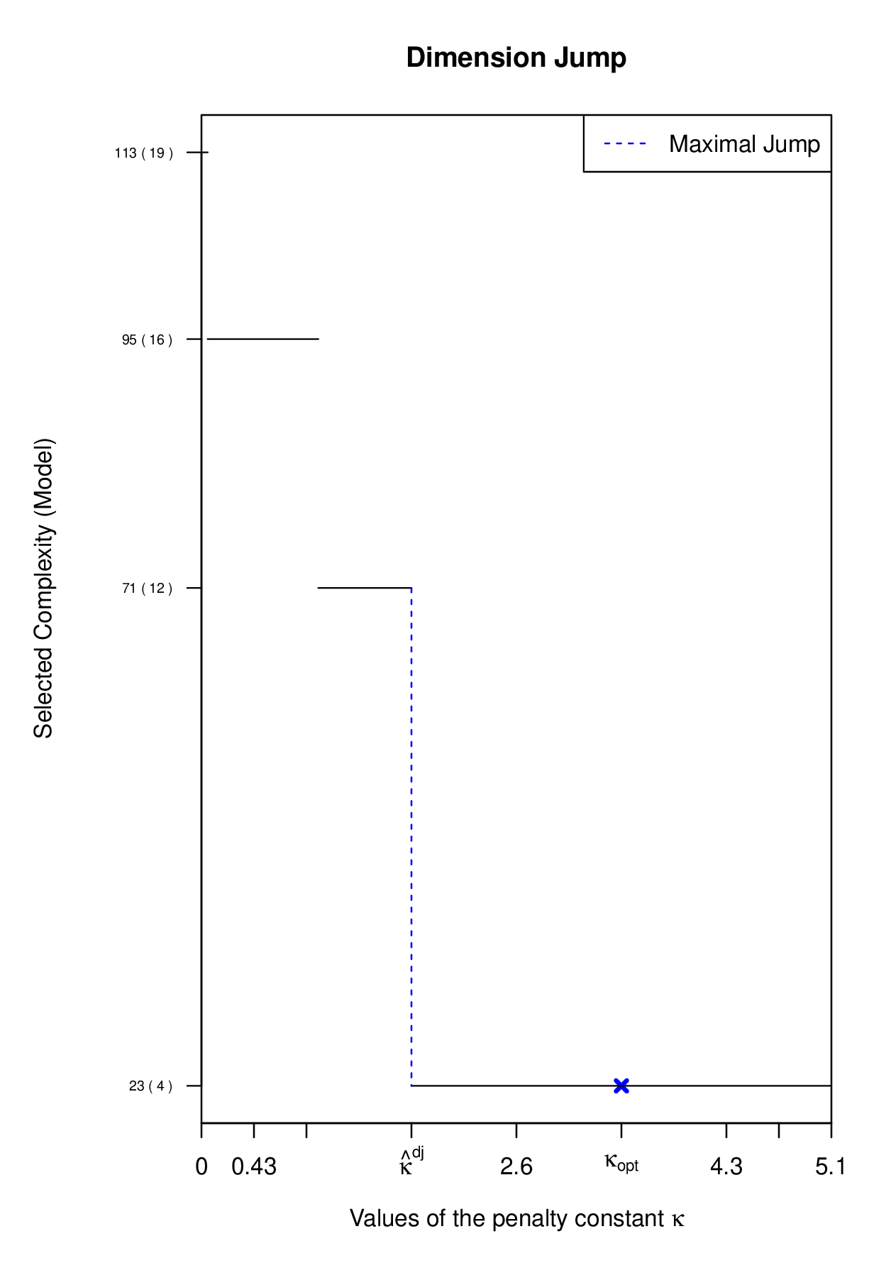
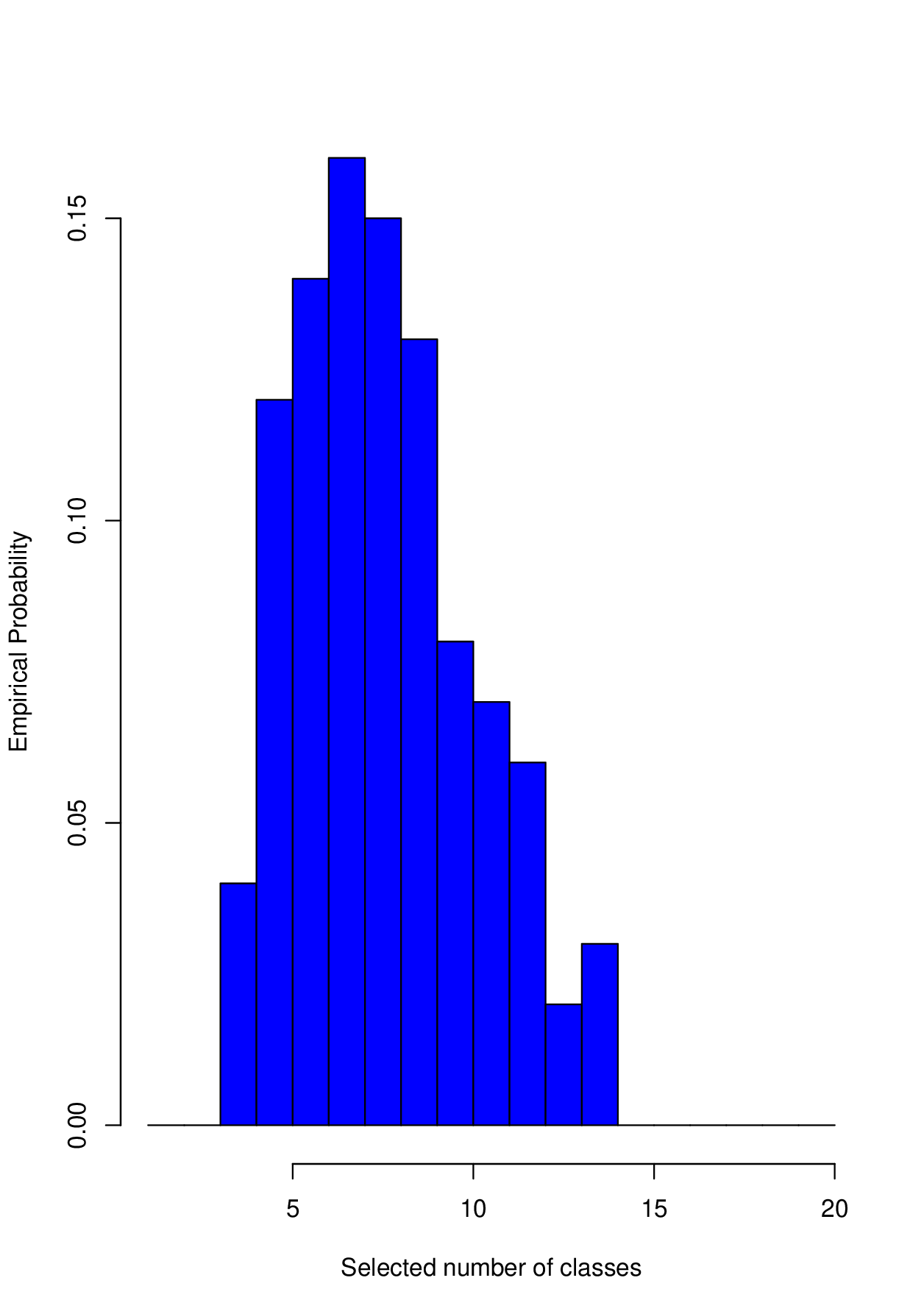
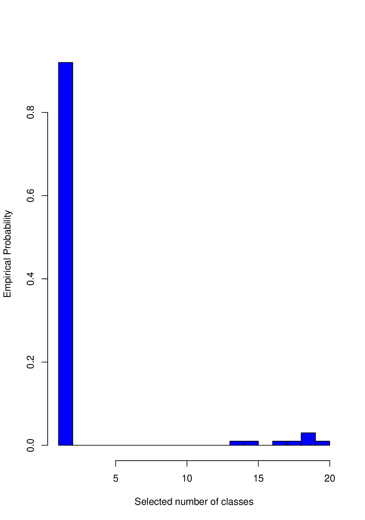
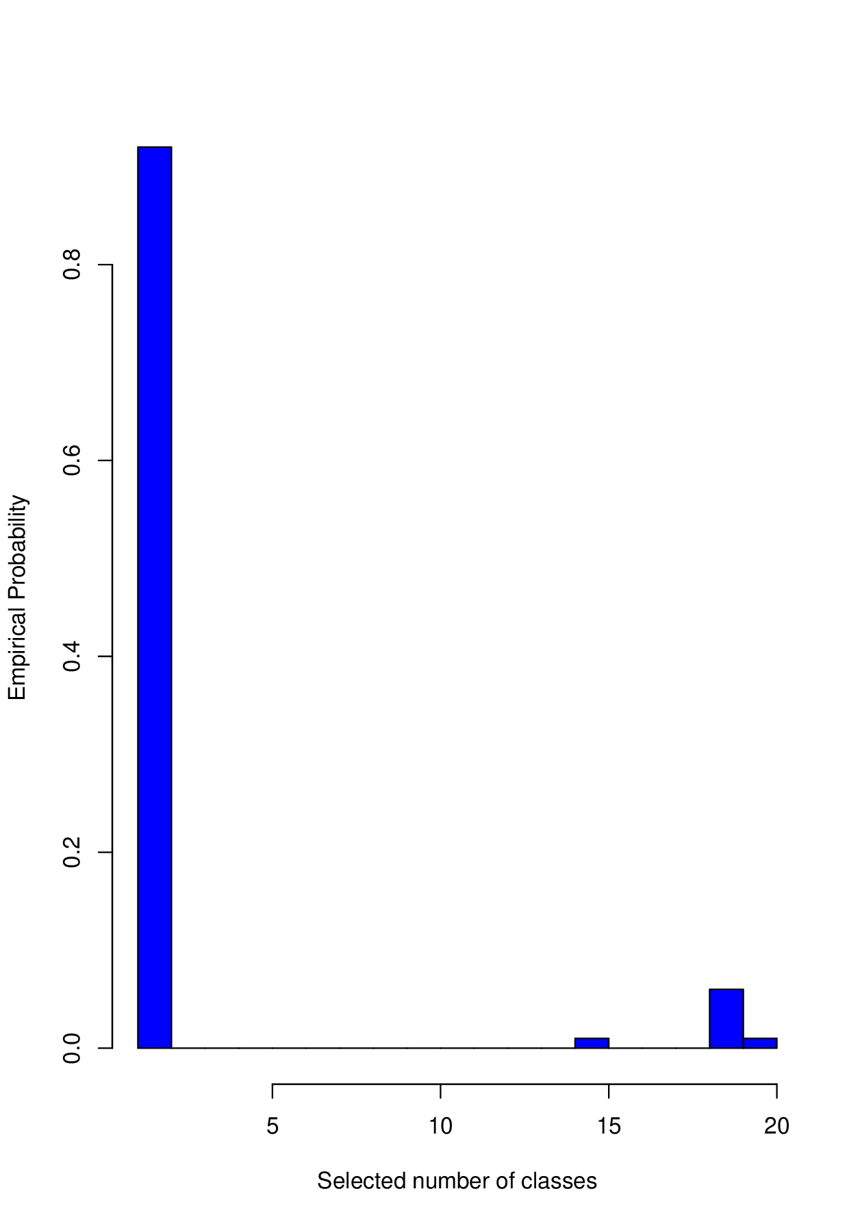
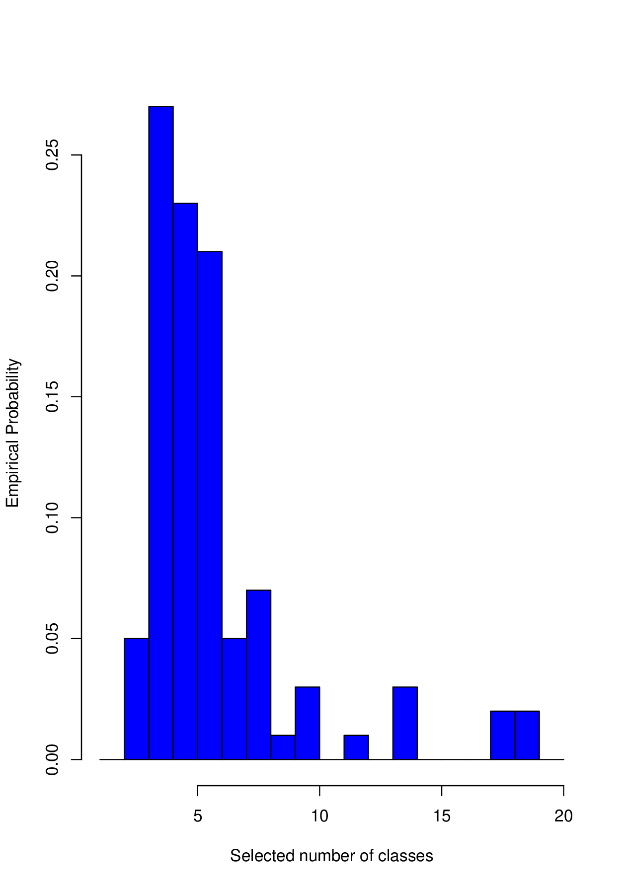
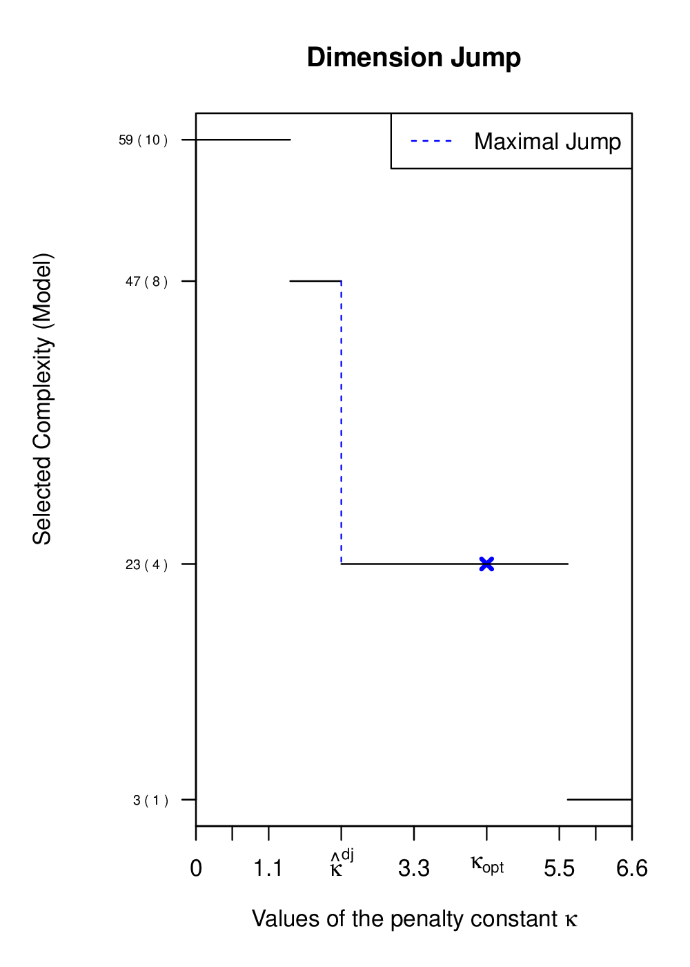
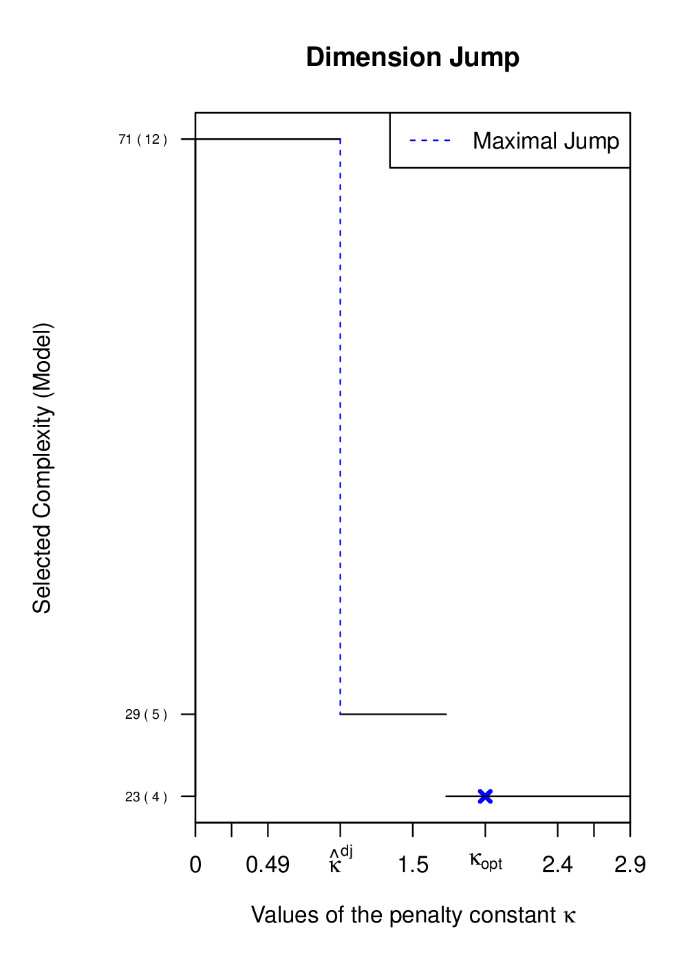
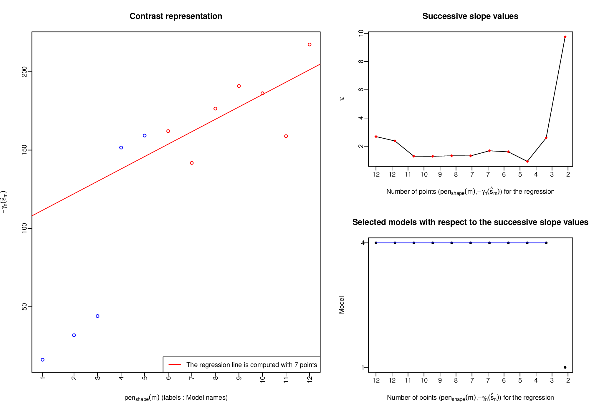
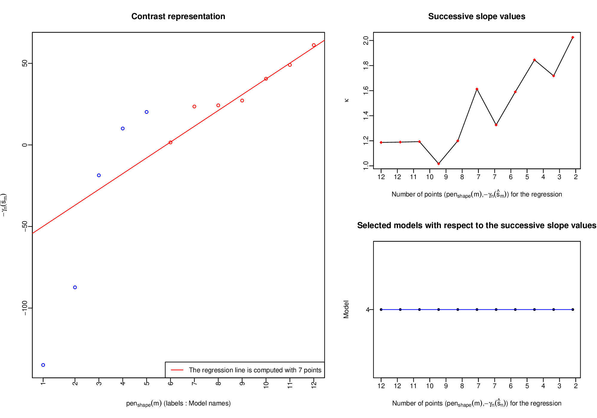
Firstly, by using the capushe (CAlibrating Penalities Using Slope HEuristics) package in R (Baudry et al., 2012), we can select the penalty coefficient, along with the number of mixture components $K$ . This heuristic comprises two possible criteria: the slope criterion and the jump criterion. The first criterion consists of computing the asymptotic slope of the log-likelihood (Figures 3 and 4), drawn according to the model dimension, and then penalizing the log-likelihood by twice the slope times the model dimension. Regarding the second criterion, one aims to represent the dimension of the selected model according to $κ$ (Figures 5 and 6), and find $\hat{κ}$ , such that if $κ < \hat{κ}$ , then the dimension of the selected model is large, and of reasonable size, otherwise. The slope heuristic prescribes then the use of $κ = 2 \hat{κ}$ . In our simulated data sets, Figures 7, 8, 9 and 10 show that the jump criterion appears to work better. The slope criterion sometimes chooses highly complex models in the WS case, with the problem exacerbated in the MS case.

Next, a close inspection shows that the bias-variance trade-off differs between the two examples. We run our experiment over $100$ trials with $K \in 𝒦 = [20]$ , using both the jump and slope criteria. The first remark is that the best choice of $K = 2$ appears to be selected with very high probability, even for large samples ( $n = 10000$ ) in the WS case. This can be observed in Figures 7(a), 7(b), 9(a) and 9(b). In the MS case, the best choice for $K$ should balance between the model approximation error term and the variance one, which is observed in Figures 8(a), 8(b), 10(a) and 10(b). Here, the larger the number of samples $n$ , the larger the value of $K$ that is selected as optimal.

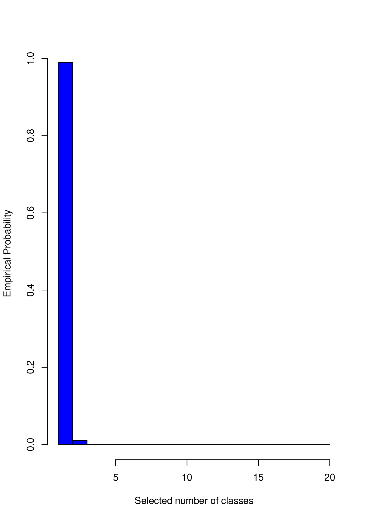
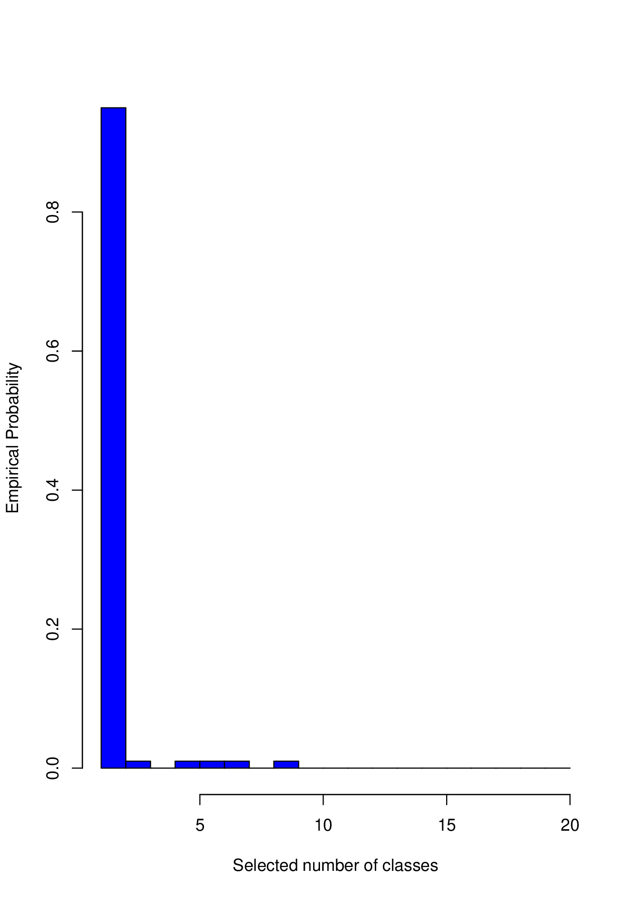
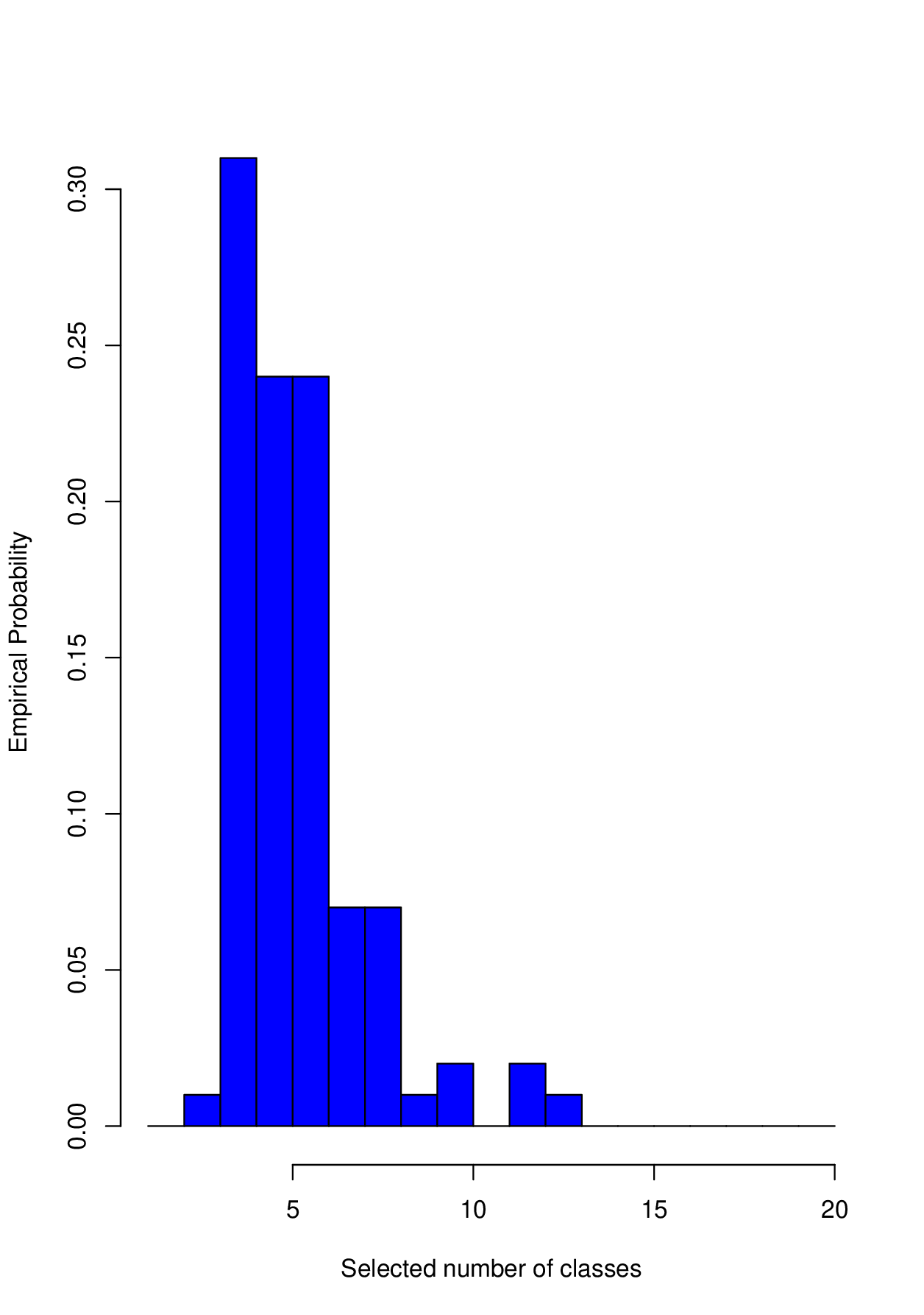
From hereon in, we only focus on the jump criterion, due to its stability regarding the choice of $K$ . We wish to measure the performances of our chosen GLoME models in term of the tensorized Kullback–Leibler divergence, $K L^{\otimes n}$ , which can not be calculated exactly in the case of Gaussian mixtures. Therefore, we evaluate the divergence using a Monte Carlo simulation, since we know the true density. We note that the variability of this randomized approximation has been demonstrated to be negligible in practice, which is also supported in the numerical experiments by Montuelle et al. (2014). More precisely, we compute the Monte Carlo approximation for the tensorized Kullback–Leibler divergence as follows. First, note that the Monte Carlo approximation for tensorized Kullback–Leibler divergence between the true model, $s_{0}^{*}$ , and the selected model $\hat{s}_{\hat{𝐦}}^{*}$ can be approximated as

	$K L^{\otimes n} (s_{0}^{}, \hat{s}_{\hat{𝐦}}^{})$	$= 𝔼_{𝐗} [\frac{1}{n} \sum_{i = 1}^{n} K L (s_{0}^{} (\cdot ∣ 𝐱_{i}), \hat{s}_{\hat{𝐦}}^{} (\cdot ∣ 𝐱_{i}))]$
		$\approx \frac{1}{n} \sum_{i = 1}^{n} K L (s_{0}^{} (\cdot ∣ 𝐱_{i}), \hat{s}_{\hat{𝐦}}^{} (\cdot ∣ 𝐱_{i}))$
		$= \frac{1}{n} \sum_{i = 1}^{n} \frac{1}{n_{y}} \sum_{j = 1}^{n_{y}} \ln (\frac{s_{0}^{} (𝐲_{i, j} ∣ 𝐱_{i})}{\hat{s}_{\hat{𝐦}}^{} (𝐲_{i, j} ∣ 𝐱_{i})}),$

where the data $𝐱_{i}, i \in [n]$ , and $(𝐲_{i, j})_{j \in [n_{y}]}$ are drawn from $s_{0}^{*} (\cdot ∣ 𝐱_{i})$ . Then, $𝔼 [K L^{\otimes n} (s_{0}^{*}, \hat{s}_{\hat{𝐦}}^{*})]$ is approximated again by averaging over $N_{t} = 100$ Monte Carlo trials. Therefore, the simulated data used for approximation can be written as $(𝐱_{i}, 𝐲_{i, j})_{t}$ with $i \in [n], j \in [n_{y}], t \in [N_{t}]$ .

Based on the approximation, Figures 11 and 12 show the box plots and the mean of the tensorized Kullback–Leibler divergence over $100$ trials, based on the jump criterion. Our boxplots confirm that the mean tensorized Kullback–Leibler divergence between $\hat{s}^{*}_{K}$ and $s_{0}^{*}$ , over $K \in {1, \dots, 20}$ number of mixture components, is always larger than the mean of tensorized Kullback–Leibler divergence between the penalized estimator $\hat{s}_{\hat{K}}^{*}$ and $s_{0}^{*}$ , which is consistent with Theorem 3.3. In particular, if the true model belongs to our nested collection, the mean tensorized Kullback–Leibler divergence seems to behave like $\frac{dim (S_{𝐦}^{*})}{2 n}$ (shown by a dotted line), which can be explained by the AIC heuristic. More precisely, we firstly assume that

S_{𝐦}^{*} = {𝒳 \times 𝒴 ∋ (𝐱, 𝐲) \mapsto s_{𝐦}^{*} : = s_{𝝍_{𝐦}^{*}} (𝐲 ∣ 𝐱) : 𝝍_{𝐦}^{*} \in 𝚿_{𝐦}^{*} \subset ℝ^{dim (S_{𝐦}^{*})}}

is identifiable and make some strong regularity assumptions on $𝝍_{𝐦}^{*} \mapsto s_{𝝍_{m}}^{*}$ . Further, we assume the existence of $dim (S_{𝐦}^{*}) \times dim (S_{𝐦}^{*})$ matrices $𝐀 (𝝍_{𝐦}^{*})$ and $𝑩 (𝝍_{𝐦}^{*})$ , which are defined as follows:

	$[𝐀 (𝝍_{𝐦}^{*})]_{k, l}$	$= 𝔼 [\frac{1}{n} \sum_{i = 1}^{n} \int \frac{- \partial^{2} \ln s_{𝝍_{𝐦}^{}}}{\partial 𝝍_{𝐦, k}^{} \partial 𝝍_{𝐦, l}^{}} (𝐲 ∣ 𝐱_{i}) s_{0}^{} (𝐲 ∣ 𝐱_{i}) d 𝐲],$
	$[𝑩 (𝝍_{𝐦}^{*})]_{k, l}$	$= 𝔼 [\frac{1}{n} \sum_{i = 1}^{n} \int \frac{\partial \ln s_{𝝍_{𝐦}^{}}}{\partial 𝝍_{𝐦, k}^{}} (𝐲 ∣ 𝐱_{i}) \frac{\partial \ln s_{𝝍_{𝐦}^{}}}{\partial 𝝍_{𝐦, l}^{}} (𝐲 ∣ 𝐱_{i}) s_{0}^{*} (𝐲 ∣ 𝐱_{i}) d 𝐲] .$

Then, the results from White (1982) and Cohen and Le Pennec (2011) imply that $𝔼 [K L^{\otimes n} (s_{0}^{*}, \hat{s}_{𝐦}^{*})]$ is asymptotically equivalent to

K L^{\otimes n} (s_{0}^{*}, s_{𝝍^{* *}_{𝐦}}) + \frac{1}{2 n} t r (𝑩 (𝝍^{* *}_{𝐦}) 𝐀 (𝝍^{* *}_{𝐦})^{- 1}),

where we defined $𝝍^{* *}_{𝐦} = a r g m i n_{s_{𝝍_{𝐦}^{*}} \in S_{𝐦}^{*}} K L^{\otimes n} (s_{0}^{*}, s_{𝝍^{*}_{m}})$ .

In particular, $𝔼 [K L^{\otimes n} (s_{0}^{*}, \hat{s}_{𝐦}^{*})]$ is asymptotically equivalent to $\frac{1}{2 n} dim (S_{𝐦}^{*})$ , whenever $s_{0}^{*}$ belongs to the model collection $S_{𝐦}^{*}$ . Furthermore, even though there is no theoretical guarantee, the slope of the mean error in the misspecified case seems also to grow at the same rate as $\frac{dim (S_{𝐦}^{*})}{2 n}$ , for large enough number of mixture components ( $K \geq 6$ in the WS case and $K \geq 9$ in the MS case).

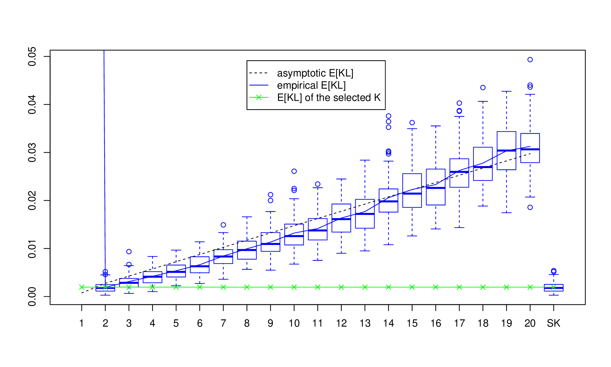
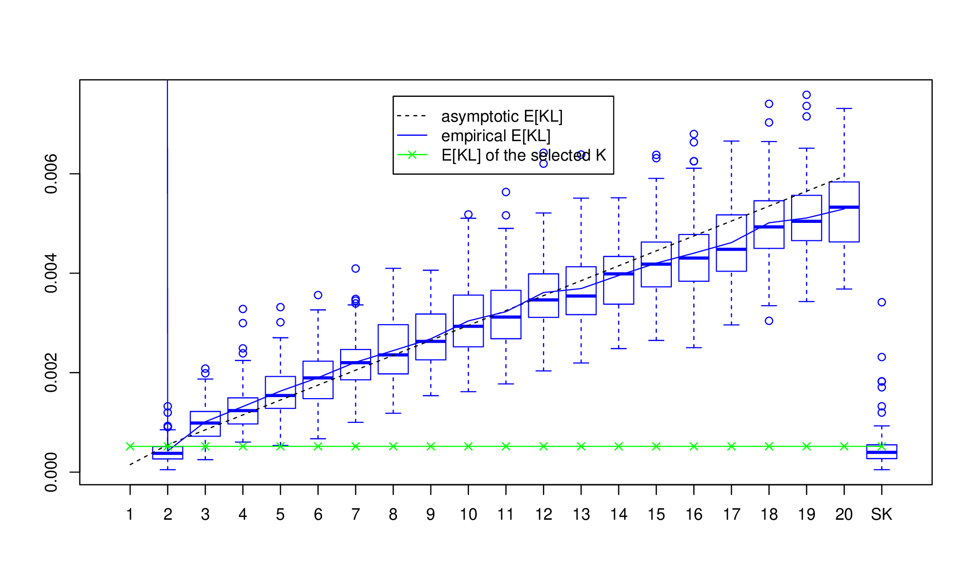
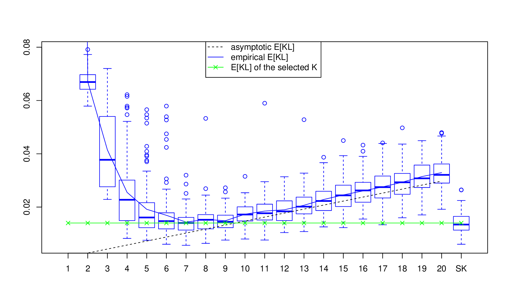
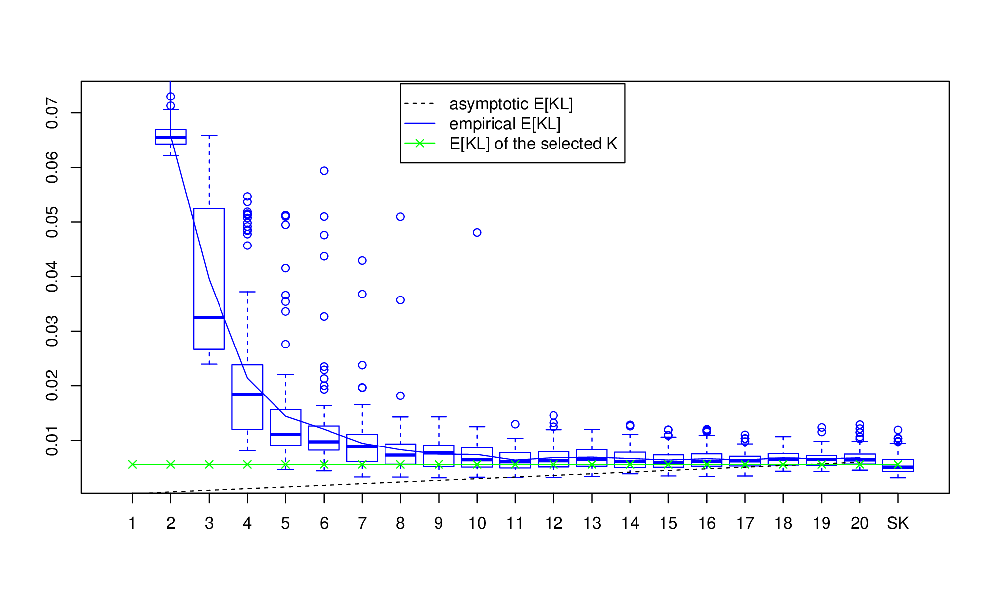
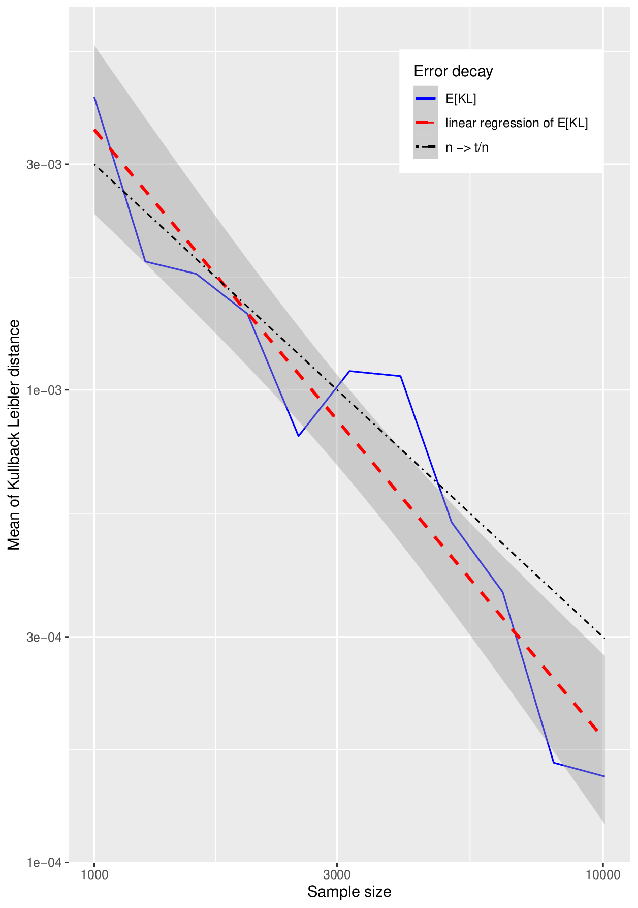
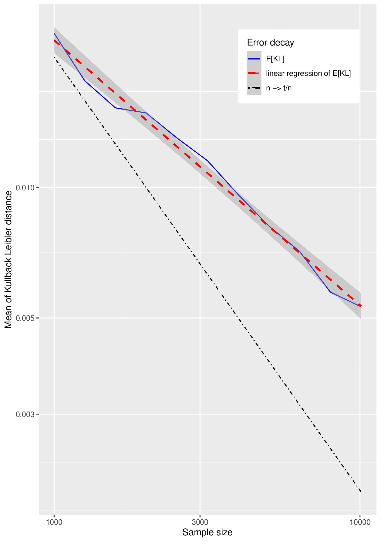
Figure 13 shows that the error decays when the sample size $n$ grows, when using the penalty based on the jump criterion. The first remark is that we observed the error decay is of order $t / n$ , as predicted in by the theory, where $t$ is some constant, as expected in the well-specified case. The rate of convergence for the misspecified case seems to be slower.

5.3 Ethanol data set

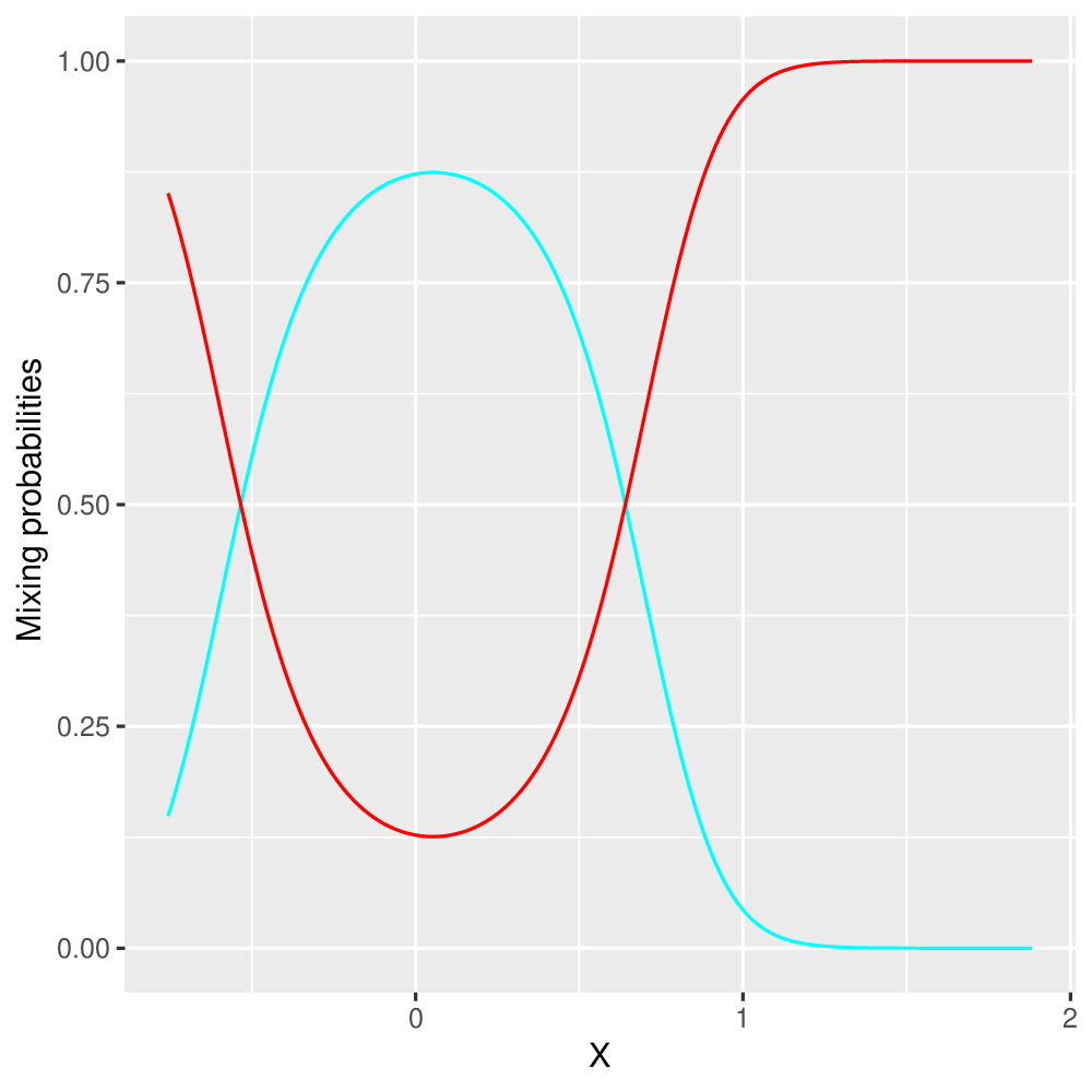
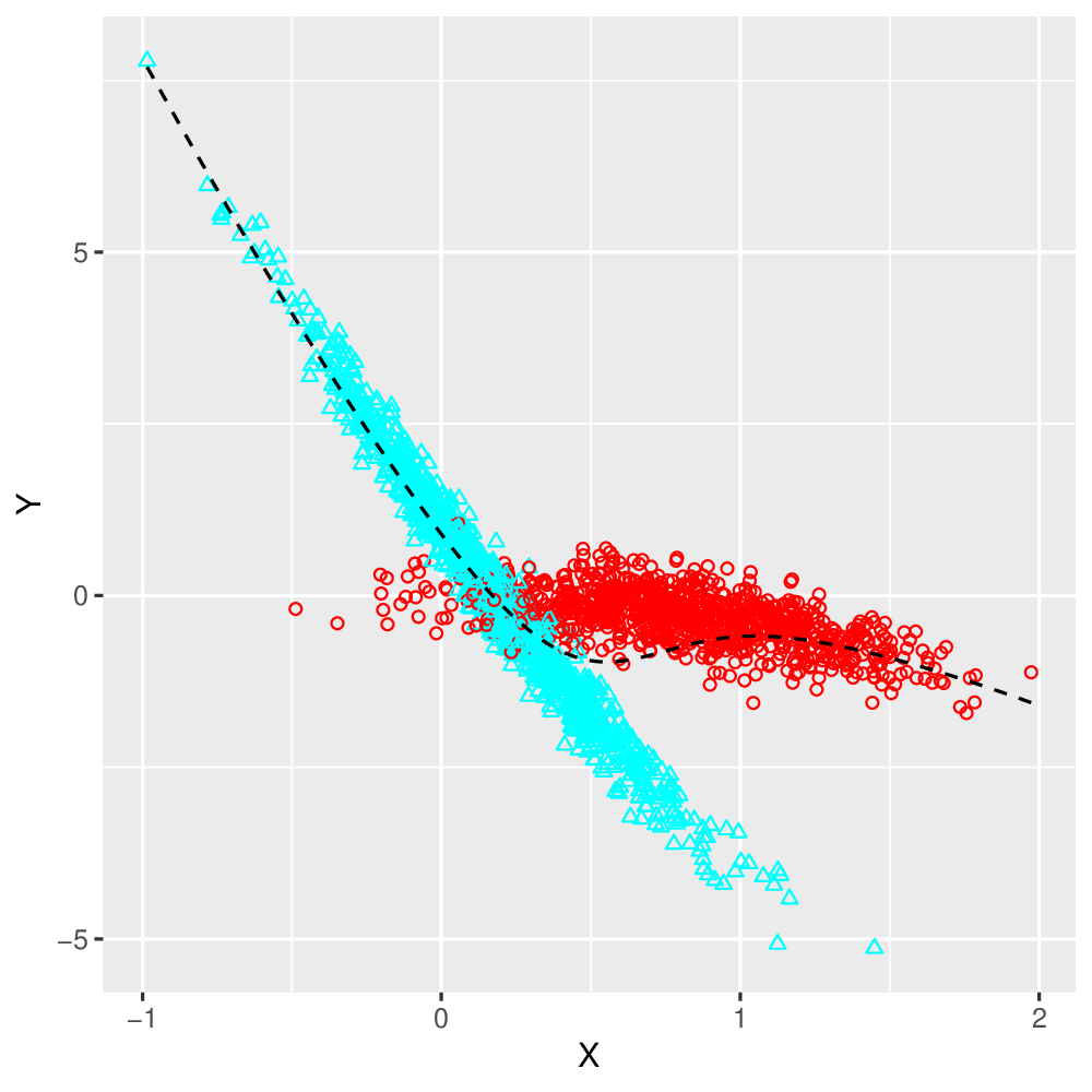
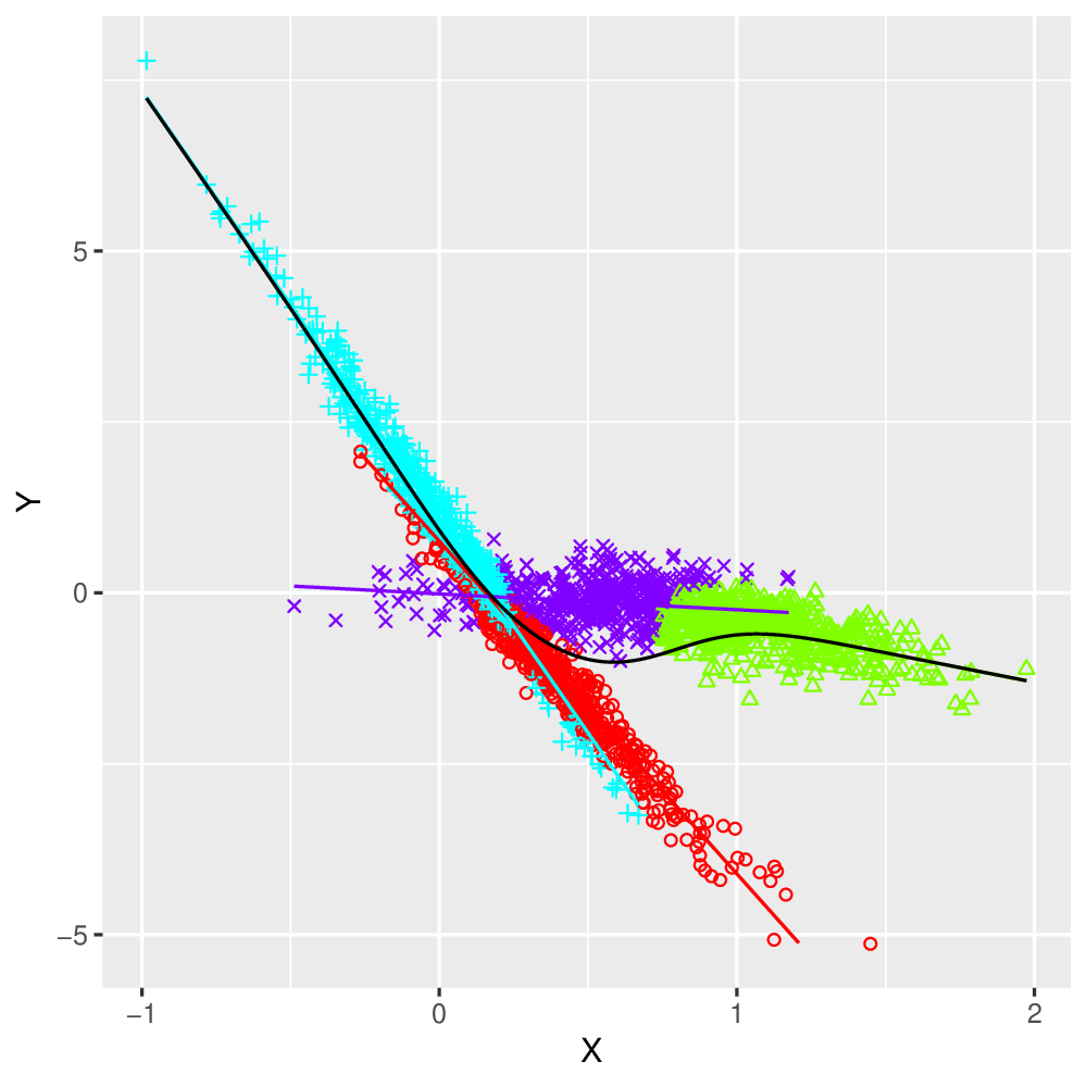
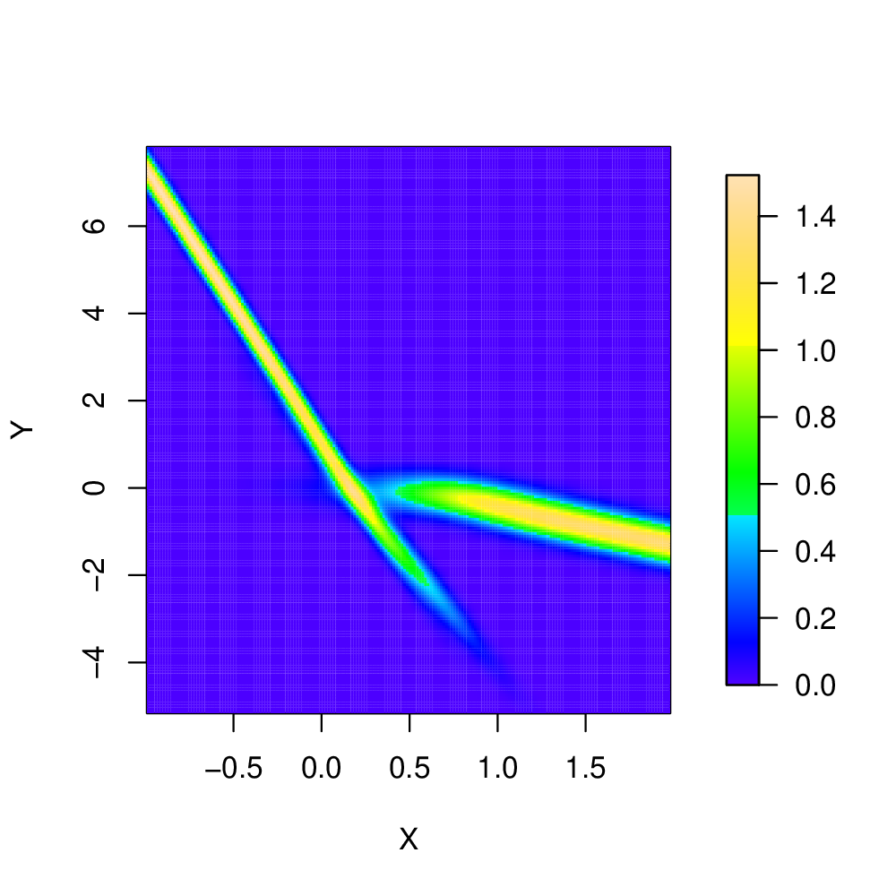
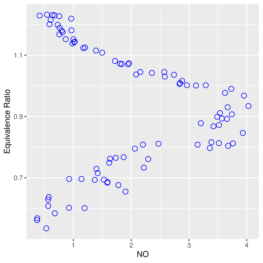
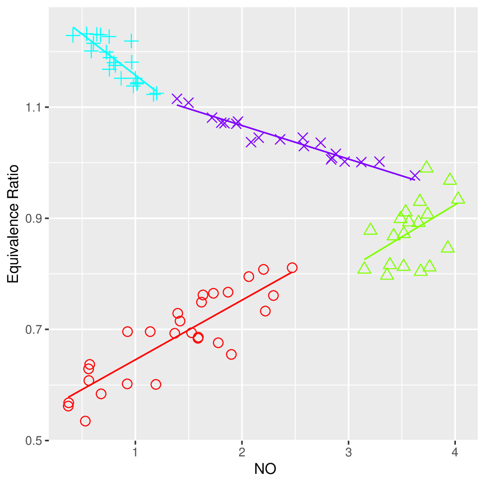
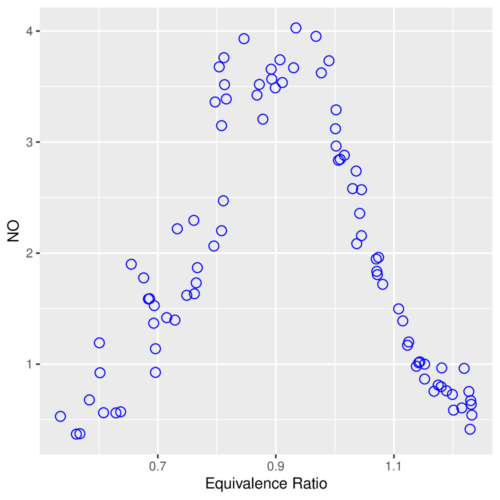
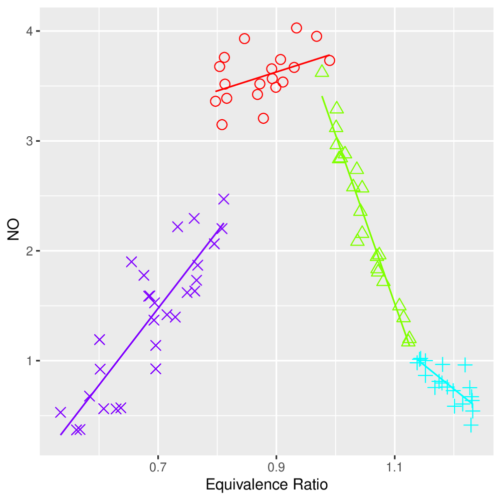
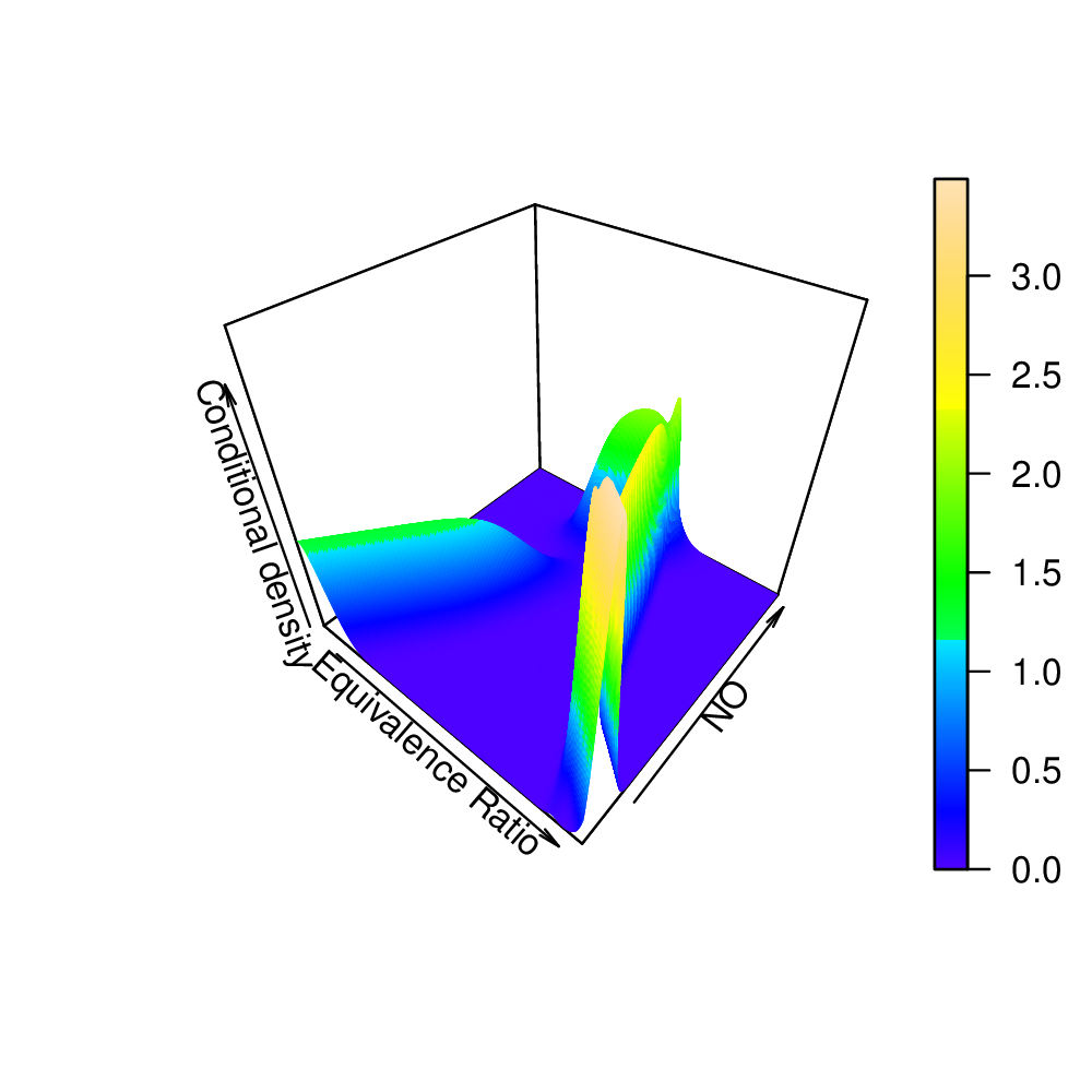
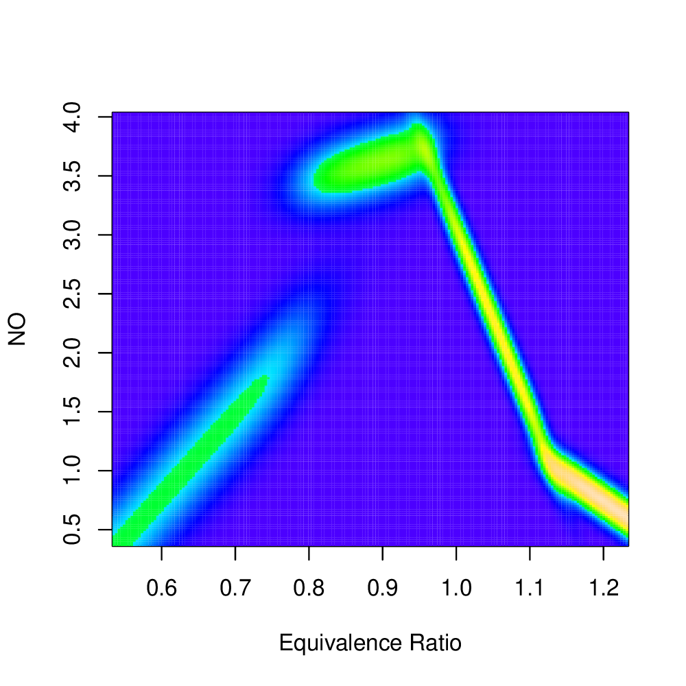
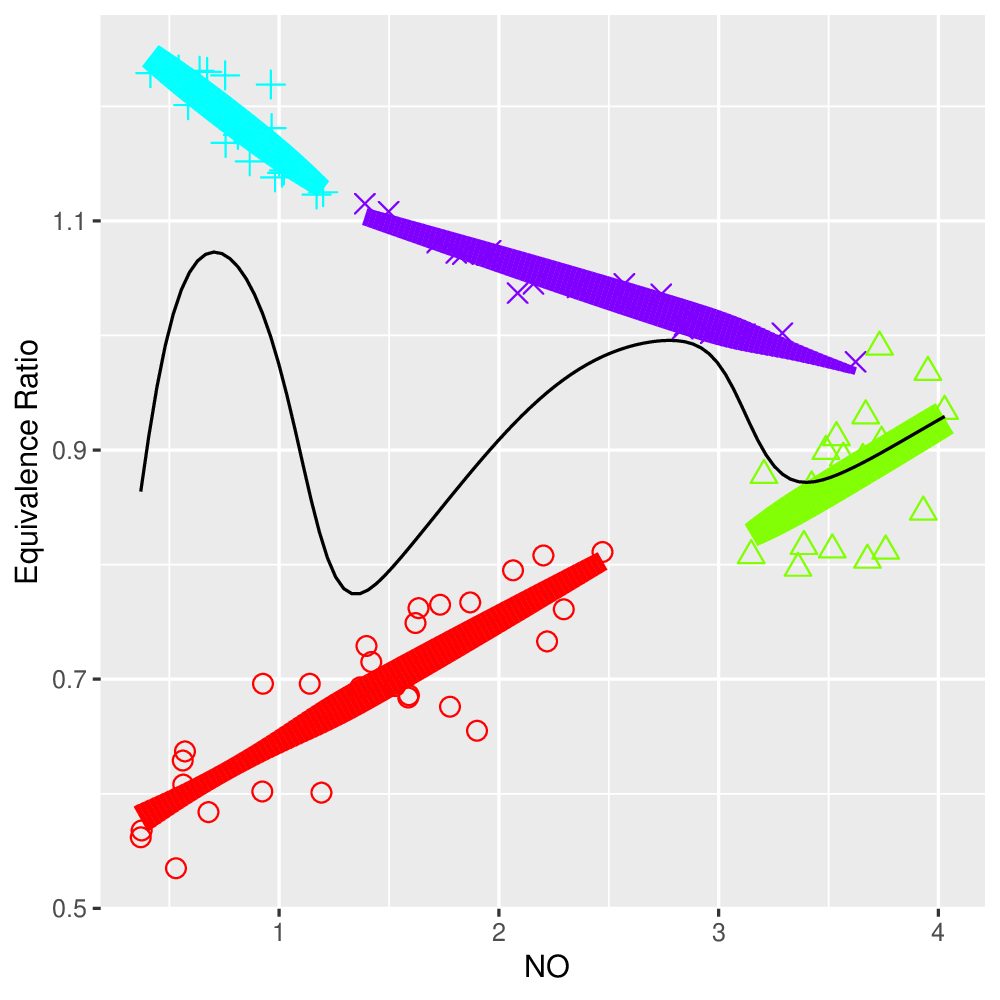
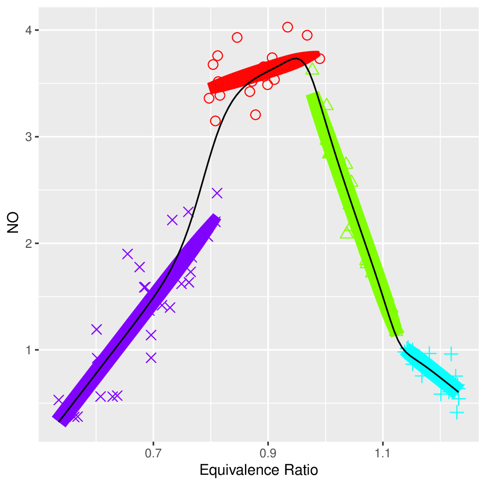
We now consider the use of GLoME models for performing clustering and regression tasks on a real data set. Following the numerical experiments from Young (2014) and Montuelle et al. (2014), we demonstrate our model on the ethanol data set of Brinkman (1981). The data comprises of 88 observations, which represent the relationship between the engine’s concentration of nitrogen oxide (NO) emissions and the equivalence ratio (ER), a measure of the air-ethanol mix, used as a spark-ignition engine fuel in a single-cylinder automobile test (Figures 18(a) and 18(e)). Our goal is then to estimate the parameters of a GLoME model, as well as the number of mixture components.

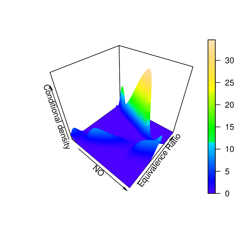
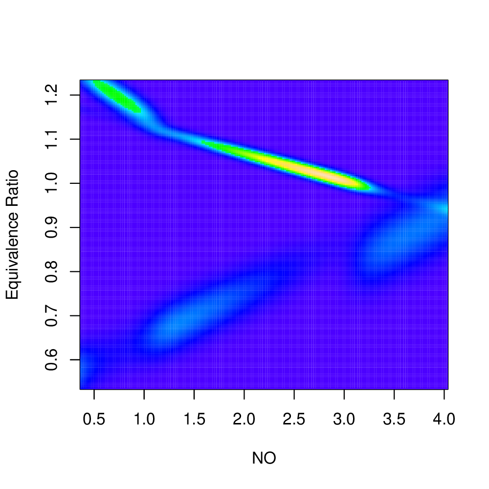
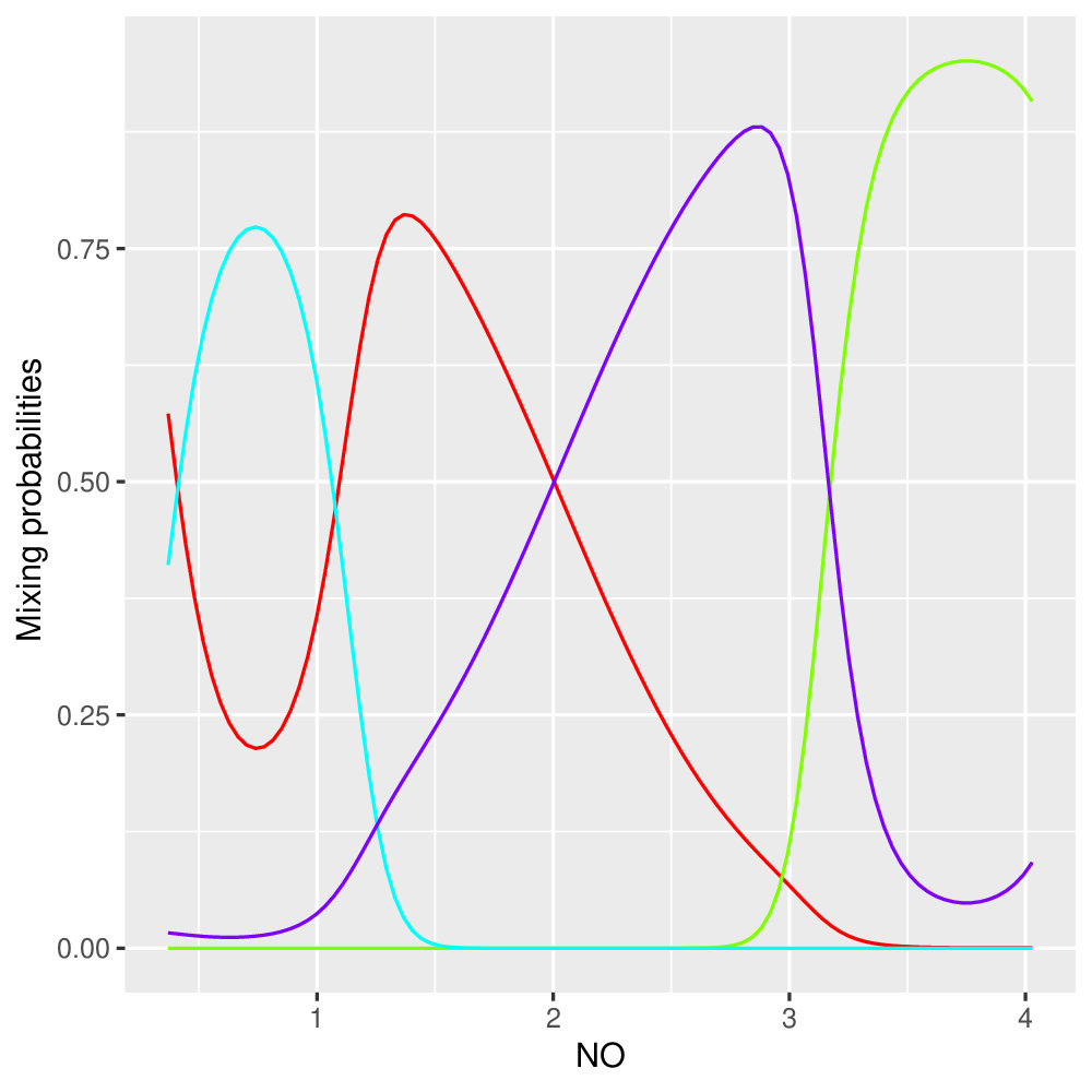
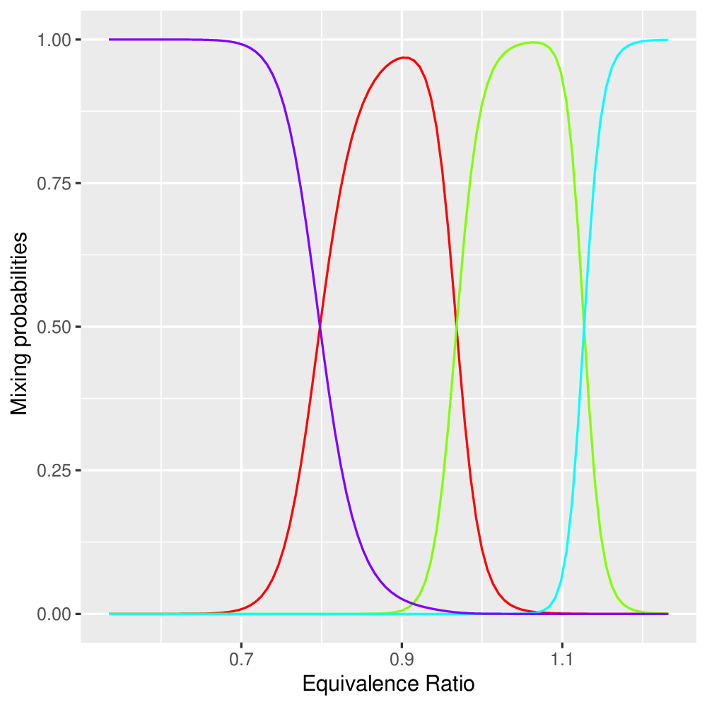
More precisely, we first use the EM algorithm from the xLLiM package to compute the forward PMLE of (2.1), for each $K \in [12]$ , on the Ethanol data set. Then, based on the slope heuristic (Figures 14, 15, 16 and 17), we select the best model. Given the estimators of the model chosen, we obtain the estimated conditional density and clustering by applying the maximum a posteriori probability (MAP) rule (Figures 18 and 19).

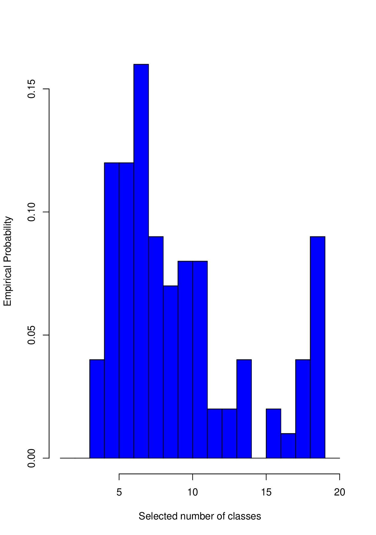
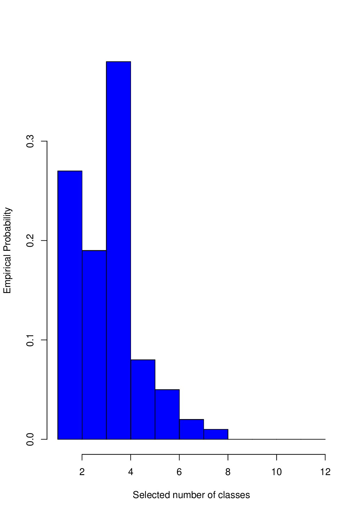
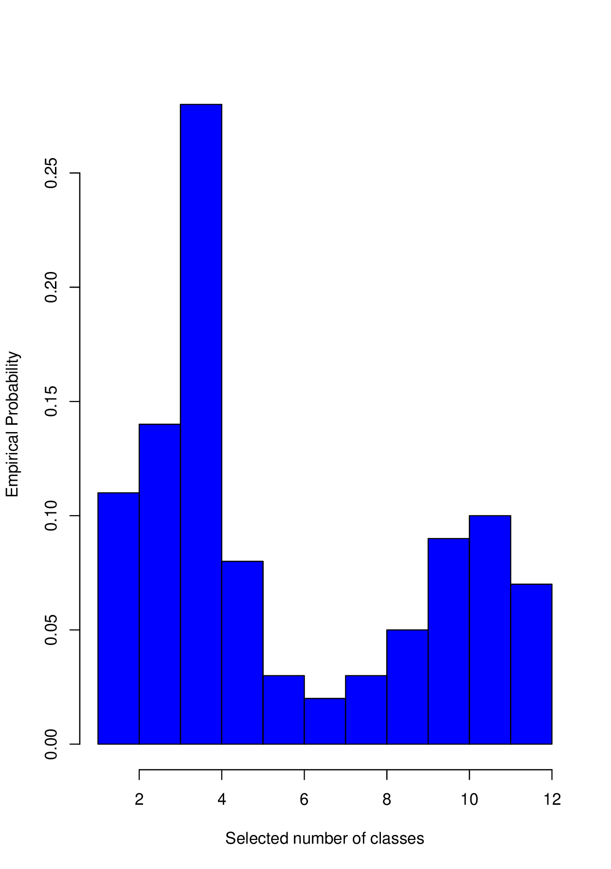
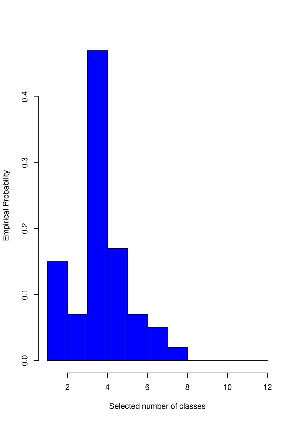
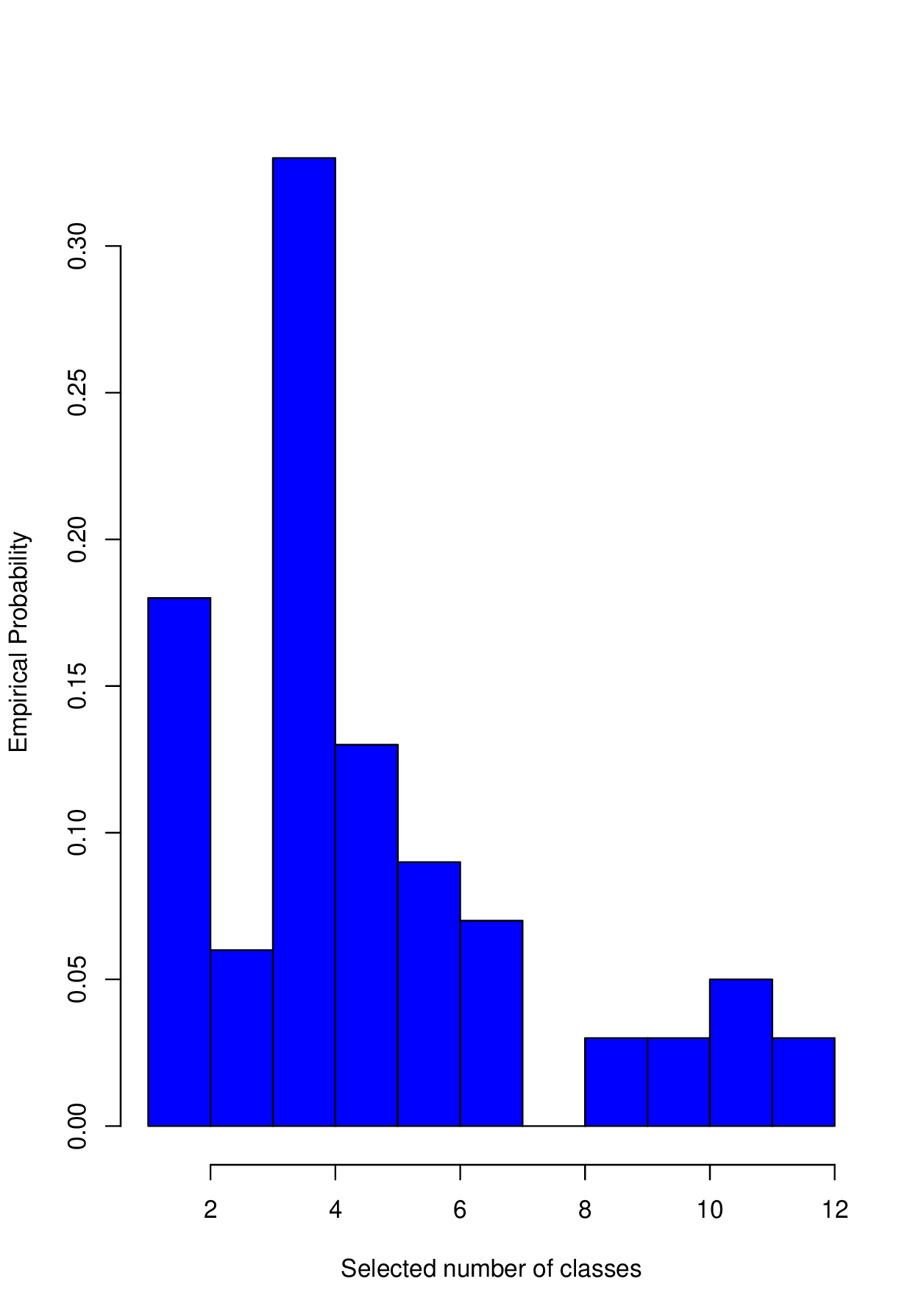
Because we only have 88 data points and $6$ parameters per class, the EM algorithm is strongly dependent on the random initialization of the parameters. One solution is that we can modify slightly that procedure in order to guarantee that at least $10$ points are assigned to each class so that the estimated parameters are more stable (cf. Montuelle et al. (2014)). In this work, we wish to investigate how well our proposed PMLE performs for detecting the best number of mixture components for the GLoME model. Thus, we run our experiment over 100 trials with different initializations for the EM algorithm. Histograms of selected values of $K$ are presented in Figures 14 and 15. Notice that it is quite unlikely that the true conditional PDF of Ethanol data set belongs to our hypothesised collection of GLoME models. In fact, this phenomenon has been observed in the MS case, Figures 7, 8, 9 and 10, on the simulated data set. We believe that this is due to the simplistic affine models used in our experiments. Furthermore, it seems that the jump criterion outperformed the slope criterion in the stability of order selection for GLoME models, as previously observed.

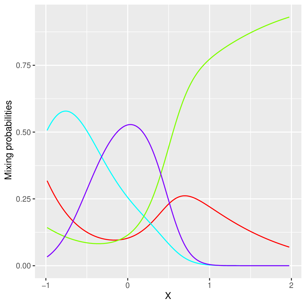
Based on the highest empirical probabilities in all situations, our procedure selects $K = 4$ components, which is consistent with the results from Montuelle et al. (2014). It is worth noting that if we consider the regression of NO with respect to ER, our proposed PMLE of GLoME performs very well for both the clustering and regression tasks (Figure 19). Here, instead of considering the variable NO as the covariate, we use it as the response variable. Then, the resulting clustering, the estimated mean function (black curve) and mixing probabilities are more easily interpretable. This is very similar to the results obtained in Montuelle et al. (2014).

6 Conclusion and perspectives

We have studied the PMLEs for GLoME and BLoME regression models. Our main contributions are to establish non-asymptotic risk bounds that take the form of finite-sample weak oracle inequalities, provided that lower bounds on the penalties hold true. We believe that our contributions help to popularize GLoME and BLoME models as well as slope heuristics, by giving some non-asymptotic theoretical foundations for model selection technique in this area and demonstrating some interesting numerical schemes and experiments. In particular, we aim to provide extensions of the current finite-sample oracle inequalities, Theorems 3.3 and 3.4, to more general frameworks where Gaussian experts are replaced by the elliptical distributions in the future work.

Some important theoretical issues regarding the tightness of the bounds of the PMLEs are still open. As per the SGaME models from Montuelle et al. (2014), we also have to deal with three potential issues: the differences of divergence on the left ( $J K L_{ρ}^{\otimes n}$ ) and the right ( $K L^{\otimes n}$ ) hand side, $C_{1} > 1$ , and the relationship between $\frac{pen (𝐦)}{n}$ and the variance. The first issue is important as in general we have $J K L_{ρ}^{\otimes n} (s_{0}, s_{𝐦}) \leq K L^{\otimes n} (s_{0}, s_{𝐦})$ . However, (2.25) ensures that the two divergences are equivalent under regularity conditions. Namely, when

sup_{𝐦 \in ℳ} sup_{s_{𝐦} \in S_{𝐦}} ∥ s_{0} / s_{𝐦} ∥_{\infty} < \infty .

Such a strong assumption is satisfied as long as $𝒳$ is compact, $s_{0}$ is compactly supported, and the regression functions are uniformly bounded, and under the condition that there is a uniform lower bound on the eigenvalues of the covariance matrices. When $s_{0} \notin (S_{𝐦})_{𝐦 \in ℳ}$ , the error bound converges to $C_{1} i n f_{s_{𝐦} \in S_{𝐦}} K L^{\otimes n} (s_{0}, s_{𝐦})$ , which may be large. Nevertheless, as we consider GLoME models, some recent results from Nguyen et al. (2019, 2021a) imply that if we take a sufficiently large number of mixture components, we can approximate a broad class of densities, and thus the term on the right hand side is small for $K$ sufficiently large. This improves the error bound even when $s_{0}$ does not belong to $S_{𝐦}$ for any $𝐦 \in ℳ$ . For the last issue, it holds that $\frac{pen (𝐦)}{n}$ is approximately proportional to the asymptotic variance, $\frac{dim (S_{𝐦})}{n}$ , in the parametric case, see its justification in Section 3.3.

Finally, it is also interesting to point out that the weak inequalities in Theorems 3.3 and 3.4 make use of different divergences and require some regularity assumptions to be considered proper oracle inequalities. To illustrate the strictness of the compactness assumption for $s_{0}$ , we only need to consider $s_{0}$ as a univariate Gaussian PDF, which obviously does not satisfy such a hypothesis. This motivates (Nguyen et al., 2020b, Theorem 3.1) to investigate an $l_{1}$ -ball model selection procedure and an $l_{1}$ -oracle inequality of SGaME with the LASSO estimator. Such an $l_{1}$ -oracle inequality can be considered as a complementary to Theorem 3.3. In particular, the most intriguing property of the $l_{1}$ -oracle inequality is that it requires only the boundedness assumption of the parameters of the model, which is also required in Theorem 3.3, as well as in Stadler et al. (2010); Meynet (2013); Devijver (2015c); Nguyen et al. (2020b). Note that such a mild assumption is quite common when working with MLE (cf. Baudry (2009); Maugis and Michel (2011a)), to tackle the problem of the unboundedness of the likelihood at the boundary of the parameter space McLachlan and Peel (2000); Redner and Walker (1984), and to prevent it from diverging. Nevertheless, by using the smaller divergence: $J K L_{ρ}^{\otimes n}$ (or more strict assumptions on $s_{0}$ and $s_{𝐦}$ , with the same divergence $K L^{\otimes n}$ as ours), Theorem 3.3 obtain a faster convergence rate of order $1 / n$ compared to $1 / \sqrt{n}$ in the $l_{1}$ -oracle inequality. Therefore, in the case where there is no guarantee of a compact support of $s_{0}$ or uniformly bounded regression functions, the $l_{1}$ -oracle inequality gives a theoretical foundation for the $l_{1}$ -ball model selection procedure, with the order of rate convergence of $1 / \sqrt{n}$ , with only the boundedness assumption on the parameter space.

Acknowledgments

TrungTin Nguyen is supported by a “Contrat doctoral” from the French Ministry of Higher Education and Research. Faicel Chamroukhi is granted by the French National Research Agency (ANR) grant SMILES ANR-18-CE40-0014. Hien Duy Nguyen is funded by Australian Research Council grant number DP180101192. This research is funded directly by the Inria LANDER project. TrungTin Nguyen also sincerely acknowledges Inria Grenoble-Rhône-Alpes Research Centre for a valuable Visiting PhD Fellowship working with STATIFY team so that this research can be completed, Erwan LE PENNEC and Lucie Montuelle for providing the simulations for the SGaME models.

Appendix A Our contributions on lemma proofs

A.1 Proof of Lemma 2.1: Inverse regression trick

We firstly aim to provide the proof of one-to-one correspondence defines the link between the inverse and forward conditional distributions not only for the special case of Gaussian distribution in (2.19) but also for elliptical distributions (cf. Cambanis et al. (1981); Fang et al. (1990)). It is worth mentioning that the multivariate normal distribution, multivariate $t$ -distribution and multivariate Laplace distribution are some instances of elliptical distributions (cf. (Frahm, 2004, Chapter 1), Hult and Lindskog (2002)). Note that a statement similar to the following has been proved in the linear regression setting in (Devijver and Perthame, 2020, Section 2.2). We include a proof for mixture of regression models, which is an extension to the aforementioned result.

A.1.1 Elliptically symmetric distributions

We will provide the proof of Lemma 2.1 by using some general results regarding elliptical distributions.

Definition A.17.

Let $𝐗$ be a $D$ -dimensional random vector. Then $𝐗$ is said to be elliptically distributed (or simply elliptical) if and only if there exist a vector $𝛍 \in ℝ^{D}$ , a positive semidefinite matrix $𝚺 \in ℝ^{D \times D}$ and a function $ϕ : ℝ^{+} \to ℝ$ such that the characteristic function $𝐭 \mapsto φ_{𝐗 - 𝛍} (𝐭)$ of $𝐗 - 𝛍$ corresponds to $𝐭 \mapsto ϕ (𝐭^{⊤} 𝚺 𝐭), 𝐭 \in ℝ^{D}$ . We write $𝐗 \sim ℰ_{D} (𝛍, 𝚺, ϕ)$ to denote that $𝐗$ is elliptical.

The function $ϕ$ is referred to as the characteristic generator of $𝑿$ . When $D = 1$ the class of elliptical distributions coincides with the class of univariate symmetric distributions. Thanks to Proposition 1 from Frahm (2004), it holds that every affinely transformed elliptical random vector is elliptically distributed. Moreover, the following stochastic representation theorem, Theorem A.18, shows that the converse is true if the transformation matrix has full rank.

Theorem A.18 (Theorem 1 from Cambanis et al. (1981)).

Let $𝐗$ be a $D$ -dimensional random vector. Then $𝐗 \sim ℰ_{D} (𝛍, 𝚺, ϕ)$ with $r a n k (𝚺) = k$ if and only if

𝐗 = 𝝁 + ℛ 𝚲 𝑼^{(k)},

where $𝐔^{(k)}$ is a $k$ -dimensional random vector uniformly distributed on the unit hypersphere with $k - 1$ dimensions $𝒮^{k - 1} = {𝐱 \in ℝ^{D} : ∥ 𝐱 ∥_{2} = 1}$ , $ℛ$ is a non-negative random variable with distribution function $F$ related to $ϕ$ being stochastically independent of $𝐔^{(k)}$ , $𝛍 \in ℝ^{D}$ and $𝚺 = 𝚲 𝚲^{⊤}$ is a rank factorization of $𝚺$ where $𝚲 \in ℝ^{D \times k}$ with $r a n k (𝚲) = k$ .

Note that via the transformation matrix $𝚲$ , the spherical random vector $𝑼^{(k)}$ produces elliptically contoured density surfaces, whereas the generating random variable $ℛ$ determines the distribution’s shape, in particular the heaviness of the distribution’s tails. Further, $𝝁$ determines the location of the random vector $𝐗$ . The matrix $𝚺$ is called the dispersion matrix or scatter matrix of $𝐗$ . Therefore, it holds that every elliptical distribution belongs to a location-scale-family (Kelker, 1970) defined by an underlying spherical standard distribution.

Example A.19 (Multivariate normal distribution).

Let $𝛍 \in ℝ^{D}$ and $𝚲 \in ℝ^{D \times k}$ such that $𝚺 : = 𝚲 𝚲^{⊤} \in ℝ^{D \times D}$ is positive definite. The random vector $𝐗 \sim Φ_{D} (𝛍, 𝚺)$ is elliptically distributed since $𝐗$ is representable as $𝐗 = 𝛍 + \sqrt{χ^{2}_{k}} 𝚲 𝐔^{(k)}$ . The underlying spherical standard distribution is the standard normal distribution. Further, since $s \mapsto \exp (- s / 2)$ is the characteristic generator for the class of normal distributions, the characteristic function of $𝐗 - 𝛍$ corresponds to $𝐭 \mapsto ϕ_{𝐗 - 𝛍} (𝐭) = \exp (- 𝐭^{⊤} 𝚺 𝐭), 𝐭 \in ℝ^{d}$ .

We next describe some important results on the conditional distributions of elliptical random vectors (cf. (Cambanis et al., 1981, Corollary 5), (Frahm, 2004, Chapter 1)).

Theorem A.20.

Let $𝐗 \sim ℰ_{D} (𝛍, 𝚺, ϕ)$ with $r a n k (𝚺) = k$ . It holds that:

(a)

$𝔼 (X) = 𝝁$ .
(b)

$var (𝐗) = \frac{𝔼 (ℛ^{2})}{k} 𝚺 = - 2 ϕ^{'} (0) 𝚺$ , if $ϕ$ is differentiable at $0$ .
(c)

The sum of independent elliptically distributed random vector with the same dispersion matrix $𝚺$ is elliptically too. Furthermore, the sum of two dependent elliptical random vectors with the same dispersion matrix, which are dependent only through their radial parts $ℛ$ , is also elliptical (Hult and Lindskog, 2002, Theorem 4.1). More precisely, let $ℛ$ and $\tilde{ℛ}$ be nonnegative random variables and let $𝐗 : = 𝝁 + ℛ 𝒁 \sim ℰ_{D} (𝝁, 𝚺, ϕ)$ and $\tilde{𝐗} : = \tilde{𝝁} + \tilde{ℛ} \tilde{𝒁} \sim ℰ_{D} (\tilde{𝝁}, 𝚺, \tilde{ϕ})$ , where $(ℛ, \tilde{ℛ})$ , $Z$ , and $\tilde{Z}$ are independent. Then $𝐗 + \tilde{𝐗} \sim ℰ_{D} (𝝁 + \tilde{𝝁}, 𝚺, ϕ^{*})$ .
(d)

Affine transformation: every affinely transformed and particularly every linearly combined elliptical random vector is elliptical, too. More formally, for any $𝐛 \in ℝ^{L}$ , $𝐀 \in ℝ^{L \times D}$ , and $𝐘 = 𝐛 + 𝐀 𝐗$ where $𝐗 = 𝝁 + ℛ 𝚲 𝑼^{(k)}$ with $𝚲 \in ℝ^{D \times k}$ , it follows that $𝐘 = ℰ_{L} (𝐛 + 𝐀 𝝁, 𝐀 𝚺 𝐀^{⊤}, ϕ)$ since

$𝐘 = 𝐛 + 𝐀 (𝝁 + ℛ 𝚲 𝑼^{(k)}) = (𝐀 𝝁 + 𝐛) + ℛ 𝐀 𝚲 𝑼^{(k)} .$ (A.1)
(e)

Marginal distribution: let $𝒫_{m} \in {0, 1}^{m \times D} (m \leq D)$ be a permutation and deletion matrix, i.e., $𝒫_{m}$ has only binary entries of $0$ ’s and $1$ ’s and $𝒫_{m} 𝒫_{m}^{⊤} = I_{m}$ . So the transformation $𝒫_{m} 𝐗 = : 𝐘$ permutes and deletes certain components of $𝐗$ such that $𝐘$ is a $k$ -dimensional random vector containing the remaining components of $𝐗$ and having a (multivariate) marginal distribution with respect to the joint distribution of $𝐗$ . Then by (A.1), we obtain $𝐘 \sim ℰ_{m} (𝒫_{m} 𝝁, 𝒫_{m} 𝚺 𝒫_{m}^{⊤}, ϕ)$ since

$𝐘 = 𝒫_{m} (𝝁 + ℛ 𝚲 𝑼^{(k)}) = 𝒫_{m} 𝝁 + ℛ 𝒫_{m} 𝚲 𝑼^{(k)} .$ (A.2)
(f)

Conditional distribution: let $𝐗 = (𝐗_{1}, 𝐗_{2})$ , where $𝐗_{1}$ is a $k$ -dimensional sub-vector of $𝐗$ , and let $𝚺 = (\begin{matrix} 𝚺_{11} & 𝚺_{12} \\ 𝚺_{21} & 𝚺_{22} \end{matrix}) \in ℝ^{D \times D}$ . Provided the conditional random vector $𝐗_{2} ∣ 𝐗_{1} = 𝐱_{1}$ exists, it is also elliptically distributed: $𝐗_{2} ∣ (𝐗_{1} = 𝐱_{1}) \sim ℰ_{D - k} (𝝁^{*}, 𝚺^{*}, ϕ^{*})$ . Moreover, it can be presented stochastically by

$𝐗_{2} ∣ (𝐗_{1} = 𝐱_{1}) = 𝝁^{*} + ℛ^{*} 𝑼^{(D - k)} Γ^{*}$

and $𝑼^{(D - k)}$ is uniformly distributed on $𝒮^{(D - k - 1)}$ , and

$ℛ^{*}$ $= ℛ \sqrt{1 - β} ∣ (ℛ \sqrt{β} 𝑼^{(k)} = 𝚺^{- 1}_{11} (𝐱_{1} - 𝝁_{1})),$

$𝝁^{*}$ $= 𝝁_{2} + 𝚺_{21} 𝚺^{- 1}_{11} (𝐱_{1} - 𝝁_{1}),$

$𝚺^{*}$ $= 𝚺_{22} - 𝚺_{21} 𝚺^{- 1}_{11} 𝚺_{12} .$

where $β \sim B e t a (k / 2, (D - k) / 2)$ and $ℛ, β, 𝑼^{(k)}$ and $𝑼^{(D - k)}$ are mutually independent, and $𝚺^{*} = (Γ^{*})^{⊤} Γ^{*}$ .

A.1.2 Relation between forward and inverse regression

Proposition 1 from Deleforge et al. (2015a), a multivariate extension of Ingrassia et al. (2012), leads to a link between GLLiM, defined in (2.18) models, and a Gaussian mixture model on the joint variable $[𝐗; 𝐘]$ . This result motivates us to establish the general proof for the relationship between forward and inverse mixture of elliptical regression models. More precisely, we consider the following generative model, conditionally on the cluster label:

[𝐗; 𝐘] ∣ (Z = k) \sim ℰ_{L + D} (𝐦_{k}, 𝐕_{k}, ϕ),

(A.3)

where $ℰ_{L + D}$ denotes an elliptical distribution of dimension $D + L$ , and are $𝐦_{k}$ and $𝐕_{k}$ its location and scale parameters, respectively.

When applying the inverse regression strategy in the context of mixture of elliptical locally-linear mapping, the key point is to account for (A.4):

𝐗 = \sum_{k = 1}^{K} 𝕀 (Z = k) (𝐀_{k} 𝐘 + 𝐛_{k} + 𝐄_{k}),

(A.4)

where $𝐀_{k} \in ℝ^{D \times L}$ and vector $𝐛_{k} \in ℝ^{D}$ , and $𝐄_{k}$ is an error term capturing both the reconstruction error due to the local affine approximation and the observation noise in $ℝ^{D}$ , into the parameterization of $𝐦_{k}$ and $𝐕_{k}$ . Given $Z = k$ , it follows from (A.3) that $𝐘$ is also elliptical distribution by using Theorem A.20 (e) and $𝐘$ can be assumed to have a location $𝐜_{k} \in ℝ^{L}$ and a scale matrix $𝚪_{k} \in ℝ^{L \times L}$ . We assume further that the error term $𝐄_{k} \sim ℰ (𝟎, ϕ_{e_{k}}, 𝚺_{k})$ is an unobserved centered elliptical random noise with residual covariance matrix $𝚺_{k}$ of type $ϕ_{e_{k}}$ , and is independent of $𝐘$ . Then, using (A.4) and Theorem A.20, we have

\begin{matrix} 𝔼 (𝐗 ∣ (Z = k)) = & 𝔼 (𝐀_{k} 𝐘 + 𝐛_{k} + 𝐄_{k}) = 𝐀_{k} 𝐜_{k} + 𝐛_{k}, \\ var (𝐗 ∣ (Z = k)) = & var (𝐀_{k} 𝐘) + var (𝐄_{k}) = 𝐀_{k} 𝚪_{k} 𝐀_{k}^{⊤} + 𝚺_{k}, \\ cov (𝐗, 𝐘 ∣ (Z = k)) = & 𝐀_{k} 𝚪_{k}, cov (𝐘, 𝐗) = cov (𝐘, 𝐀_{k} 𝐘) = 𝚪_{k}^{⊤} 𝐀_{k}^{⊤}, \\ 𝐦_{k} = & [\begin{matrix} 𝐀_{k} 𝐜_{k} + 𝐛_{k} \\ 𝐜_{k} \end{matrix}], \\ 𝐕_{k} = & [\begin{matrix} 𝚺_{k} + 𝐀_{k} 𝚪_{k} 𝐀_{k}^{⊤} & 𝐀_{k} 𝚪_{k} \\ (𝐀_{k} 𝚪_{k})^{⊤} & 𝚪_{k} \end{matrix}] . \end{matrix}

(A.5)

Note that in the forward and inverse regression problems of elliptical locally-linear mapping (containing the Gaussian case (2.12), (2.13), (2.17) and (2.16)), by using Theorem A.20, the joint distribution defined in (A.3) allows us to consider a mixture of linear regression problem, characterized by the following marginal and conditional distributions:

$𝐗 ∣ (Z = k)$	$\sim ℰ_{D} (𝐜_{k}^{}, 𝚪_{k}^{}, ϕ),$	(A.6)
$𝐘 ∣ (𝐗, Z = k)$	$= 𝐀^{}_{k} 𝐗 + 𝐛^{}_{k} + 𝐄^{*}_{k},$	(A.7)
$𝐘 ∣ (Z = k)$	$\sim ℰ_{D} (𝐜_{k}, 𝚪_{k}, ϕ),$	(A.8)
$𝐗 ∣ (𝐘, Z = k)$	$= 𝐀_{k} 𝐘 + 𝐛_{k} + 𝐄_{k},$	(A.9)

where $𝐄_{k} \sim ℰ (𝟎, ϕ_{e_{k}}, 𝚺_{k})$ and $𝐄^{*}_{k} \sim ℰ (𝟎, ϕ_{e^{*}_{k}}, 𝚺^{*}_{k})$ .

Then, we claim that the joint distribution, defined in (A.3) and (A.5), leads to the marginal and the conditional distributions of Equations A.6 to A.9 and to a mapping between their mean and variance parameters. Indeed, by using conditioning properties of elliptical distributions, see more in Theorem A.20, implies the following marginal for $𝐗$ and conditional distribution for $𝐘$ given $𝐗$ as follows:

	$𝐗 ∣ (Z = k)$	$\sim ℰ_{D} (𝐀_{k} 𝐜_{k} + 𝐛_{k}, 𝚺_{k} + 𝐀_{k} 𝚪_{k} 𝐀_{k}^{⊤}, ϕ),$		(A.10)
	$𝐘 ∣ (𝐗, Z = k)$	$\sim ℰ_{L} (𝒎^{y x}_{k}, 𝚺^{y x}_{k}, \tilde{ϕ}),$		(A.11)

where the explicit expression of the characteristic function $\tilde{ϕ}$ can be found in (Cambanis et al., 1981, Corollary 5), and

	$𝒎^{y x}_{k}$	$= 𝐜_{k} + 𝚪_{k}^{⊤} 𝐀_{k}^{⊤} (𝚺_{k} + 𝐀_{k} 𝚪_{k} 𝐀_{k}^{⊤})^{- 1} (𝐗 - 𝐀_{k} 𝐜_{k} - 𝐛_{k}),$
	$𝚺^{y x}_{k}$	$= 𝚪_{k} - 𝚪_{k}^{⊤} 𝐀_{k}^{⊤} (𝚺_{k} + 𝐀_{k} 𝚪_{k} 𝐀_{k}^{⊤})^{- 1} 𝐀_{k} 𝚪_{k} = (𝚪_{k}^{- 1} + 𝐀_{k}^{⊤} 𝚺_{k}^{- 1} 𝐀_{k})^{- 1},$

with the fact that the last equality is the Woodbury matrix identity. Note that the locations and scale matrices of the conditional distribution do not depend upon the third parameter of the joint distribution, and consequently, we do not describe the explicit expression for $\tilde{ϕ}$ . We then utilize again the Woodbury matrix identity and the symmetric property of $𝚪$ to identify (A.6) and (A.7) with (A.10) and (A.11), respectively, which implies the following important connections:

	$𝐜_{k}^{*}$	$= 𝐀_{k} 𝐜_{k} + 𝐛_{k}, 𝚪_{k}^{} = 𝚺_{k} + 𝐀_{k} 𝚪_{k} 𝐀_{k}^{⊤}, 𝚺^{}_{k} = (𝚪_{k}^{- 1} + 𝐀_{k}^{⊤} 𝚺_{k}^{- 1} 𝐀_{k})^{- 1},$
	$𝐀_{k}^{*}$	$= 𝚪_{k}^{⊤} 𝐀_{k}^{⊤} (𝚺_{k} + 𝐀_{k} 𝚪_{k} 𝐀_{k}^{⊤})^{- 1}$
		$= 𝚪_{k}^{⊤} 𝐀_{k}^{⊤} 𝚺^{- 1}_{k} - 𝚪_{k}^{⊤} 𝐀_{k}^{⊤} 𝚺^{- 1}_{k} 𝐀_{k} (𝚪_{k}^{- 1} + 𝐀_{k}^{⊤} 𝚺^{- 1}_{k} 𝐀_{k})^{- 1} 𝐀_{k}^{⊤} 𝚺^{- 1}_{k}$
		$= [𝚪_{k} (𝚪_{k}^{- 1} + 𝐀_{k}^{⊤} 𝚺^{- 1}_{k} 𝐀_{k}) - 𝚪_{k} 𝐀_{k}^{⊤} 𝚺^{- 1}_{k} 𝐀_{k}] (𝚪_{k}^{- 1} + 𝐀_{k}^{⊤} 𝚺^{- 1}_{k} 𝐀_{k})^{- 1} 𝐀_{k}^{⊤} 𝚺^{- 1}_{k}$
		$= (𝚪_{k}^{- 1} + 𝐀_{k}^{⊤} 𝚺^{- 1}_{k} 𝐀_{k})^{- 1} 𝐀_{k}^{⊤} 𝚺^{- 1}_{k} = 𝚺^{*}_{k} 𝐀_{k}^{⊤} 𝚺^{- 1}_{k},$
	$𝐛_{k}^{*}$	$= 𝐜_{k} + 𝚪_{k}^{⊤} 𝐀_{k}^{⊤} (𝚺_{k} + 𝐀_{k} 𝚪_{k} 𝐀_{k}^{⊤})^{- 1} (- 𝐀_{k} 𝐜_{k} - 𝐛_{k})$
		$= 𝐜_{k} + (𝚪_{k}^{- 1} + 𝐀_{k}^{⊤} 𝚺^{- 1}_{k} 𝐀_{k})^{- 1} 𝐀_{k}^{⊤} 𝚺^{- 1}_{k} (- 𝐀_{k} 𝐜_{k} - 𝐛_{k})$
		$= (𝚪_{k}^{- 1} + 𝐀_{k}^{⊤} 𝚺^{- 1}_{k} 𝐀_{k})^{- 1} [(𝚪_{k}^{- 1} + 𝐀_{k}^{⊤} 𝚺^{- 1}_{k} 𝐀_{k}) 𝐜_{k} + 𝐀_{k}^{⊤} 𝚺^{- 1}_{k} (- 𝐀_{k} 𝐜_{k} - 𝐛_{k})]$
		$= 𝚺_{k}^{*} (𝚪_{k}^{- 1} 𝐜_{k} - 𝐀_{k}^{⊤} 𝚺_{k}^{- 1} 𝐛_{k}) .$

Therefore, the desired results then are obtained by using the fact that the multivariate normal distribution not only has the property of having Gaussian marginal and conditional distributions (Bishop, 2006, Sections 2.3.1 and 2.3.2) but also belongs to elliptical distributions (detailed in Example A.19). Furthermore, it should be stressed that several versions of multivariate $t$ -distributions (e.g., Section 5.5, page 94 of Kotz and Nadarajah (2004), Ding (2016)) have the previous property. This leads to the inverse regression model based on the multivariate $t$ -distributions (Perthame et al., 2018). It will be interesting to find other sub-classes of elliptically contoured distributions that have the closedness property on marginal and conditional distribution so that the previous inverse regression trick can be applied.

A.2 Proof of Lemma 4.9: Bracketing entropy of Gaussian gating networks

Note that the first inequality of Lemma 4.9 comes from (Montuelle et al., 2014, Lemma 4) and describes relationship between the bracketing entropy of $𝒫_{K}$ and the entropy of $𝒲_{K}$ . Therefore, Lemma 4.9 is obtained by proving that there exists a constant $C_{𝒲_{K}}$ such that $\forall δ \in (0, 2]$ ,

ℋ_{d_{∥ sup ∥_{\infty}}} (δ, 𝒲_{K})

\leq dim (𝒲_{K}) (C_{𝒲_{K}} + \ln (\frac{1}{δ})),

(A.12)

where $dim (𝒲_{K}) = K - 1 + K L + K \frac{L (L + 1)}{2}$ .

In order to establish the proof for (A.12), we have to construct firstly the $δ_{𝝅}$ -covering $𝚷_{K - 1, 𝝎}$ of $𝚷_{K - 1}$ via Lemma A.21, which is proved in Section A.2.1.

Lemma A.21 (Covering number of probability simplex with maximum norm).

Given any $δ_{𝛑} > 0$ , any $𝛑 \in 𝚷_{K - 1}$ , we can choose $\hat{𝛑} \in 𝚷_{K - 1, 𝛚}$ , an $δ_{𝛑}$ -covering of $𝚷_{K - 1}$ , so that $\max_{k \in [K]} | π_{k} - \hat{𝛑}_{k} | \leq δ_{𝛑}$ . Furthermore, it holds that

𝒩 (δ_{𝝅}, 𝚷_{K - 1}, ∥ \cdot ∥_{\infty}) \leq \frac{K (2 π e)^{K / 2}}{δ^{K - 1}_{𝝅}} .

(A.13)

Then, by definition of the covering number, (A.12) is obtained immediately via Lemma A.22, which controls the covering number of $𝒲_{K}$ and is proved in Section A.2.2.

Lemma A.22.

Given a bounded set $𝒴$ in $ℝ^{L}$ such that $𝒴 = {𝐲 \in ℝ^{L} : ∥ 𝐲 ∥_{\infty} \leq C_{𝒴}}$ , it holds that $𝒲_{K}$ has a covering number satisfied $𝒩 (δ, 𝒲_{K}, d_{∥ sup ∥_{\infty}}) \leq C δ^{- dim (𝒲_{K})}$ , for some constant $C$ .

Indeed, Lemma A.22 implies the desired result by noting that

	$ℋ_{d_{∥ sup ∥_{\infty}}} (δ, 𝒲_{K})$	$= \ln 𝒩 (δ, 𝒲_{K}, d_{∥ sup ∥_{\infty}}) \leq \ln [\frac{C}{δ^{dim (𝒲_{K})}}]$
		$= dim (𝒲_{K}) [\frac{1}{dim (𝒲_{K})} \ln C + \ln (\frac{1}{δ})]$
		$= dim (𝒲_{K}) (C_{𝒲_{K}} + \ln (\frac{1}{δ})) .$

A.2.1 Proof of Lemma A.21

Note that (Genovese and Wasserman, 2000, Lemma 2) provide a result for controlling a $δ_{𝝅}$ -Hellinger bracketing of $𝚷_{K - 1}$ . However, such result can not be applied for our Lemma A.21 since they use $δ_{𝝅}$ -Hellinger bracketing entropy while we use $δ_{𝝅}$ -covering number for the probability complex with maximum norm.

Given any $𝝅 = (π_{k})_{k \in [K]} \in 𝚷_{K - 1}$ , let $𝝃 = (𝝃_{k})_{k \in [K]}$ where $𝝃_{k} = \sqrt{π_{k}}, \forall k \in [K]$ . Then $𝝅 \in 𝚷_{K - 1}$ if and only if $𝝃 \in Q^{+} \cap U$ , where $U$ is the surface of the unit sphere and $Q^{+}$ is the positive quadrant of $ℝ^{K}$ . Next, we divide the unit cube in $ℝ^{K}$ into disjoint cubes with sides parallel to the axes and sides of length $δ_{𝝅} / \sqrt{K}$ . Let $(𝐂_{j})_{j \in [N]}$ is the subset of these cubes that have non-empty intersection with $Q^{+} \cap U$ . For any $j \in [N]$ , let $𝝂_{j} = (𝝂_{j, k})_{k \in [K]}$ be the center of the cube $𝐂_{j}$ and $𝝂^{2}_{j} = (𝝂^{2}_{j, k})_{k \in [K]}$ .

Then ${𝝂_{j}}_{j \in [N]}$ is a $δ_{𝝅} / (2 \sqrt{K})$ -covering of $Q^{+} \cap U$ , since we have for any $𝝃 = (𝝃_{k})_{k \in [K]} \in Q^{+} \cap U$ , there exists $j_{0} \in [N]$ such that $𝝃 \in 𝐂_{j_{0}}$ , and

∥ 𝝃 - 𝝂_{j_{0}} ∥_{\infty} = \max_{k \in [K]} | 𝝃_{k} - 𝝂_{j_{0}, k} | \leq \frac{δ_{𝝅}}{2 \sqrt{K}} .

(A.14)

Therefore, it follows that $𝚷_{K - 1, 𝝎} : = {𝝂^{2}_{j}}_{j \in [N]}$ is a $δ_{𝝅}$ -covering of $𝚷_{K - 1}$ , since for any $𝝅 = (π_{k})_{k \in [K]} \in 𝚷_{K - 1}$ , (A.14) leads to the existence of $j_{0} \in [N]$ , such that

	$∥ 𝝅 - 𝝂^{2}_{j_{0}} ∥_{\infty}$	$= \max_{k \in [K]} \| 𝝃^{2}_{k} - 𝝂^{2}_{j_{0}, k} \| = \max_{k \in [K]} {\| 𝝃_{k} - 𝝂_{j_{0}, k} \| \| 𝝃_{k} + 𝝂_{j_{0}, k} \|}$
		$\leq \frac{δ_{𝝅}}{2 \sqrt{K}} \max_{k \in [K]} \| 𝝃_{k} + 𝝂_{j_{0}, k} \| \leq \frac{δ_{𝝅}}{\sqrt{K}} \leq δ_{𝝅},$

where we used the fact that $\max_{k \in [K]} | 𝝃_{k} + 𝝂_{j_{0}, k} | \leq 2$ . Now, it remains to count the number of cubes $N$ . Let $𝒯_{a} = {𝒛 \in Q^{+} : ∥ 𝒛 ∥_{2} \leq a}$ and let $𝒞 = ⋃_{j \in [N]} 𝐂_{j}$ . Note that $𝒞 \subset 𝒯_{1 + δ_{𝝅}} - 𝒯_{1 - δ_{𝝅}} \equiv 𝒯$ , and so

Volume (𝒯) \geq Volume (𝒞) = N (\frac{δ_{𝝅}}{\sqrt{K}})^{K} .

Note that here we use the notation $π$ for the Archimedes’ constant, which differs from $𝝅 = (π_{k})_{k \in [K]}$ for the mixing proportion of the GLoME model. Then, we define $𝒱_{K} (a) = a^{K} π^{K / 2}$ as the volume of a sphere of radius $a$ . Since $z! \geq z^{z} e^{- z}$ and $(1 + δ_{𝝅})^{K} - (1 - δ_{𝝅})^{K} = K \int_{1 - δ_{𝝅}}^{1 + δ_{𝝅}} z^{K - 1} d z \leq 2 δ_{𝝅} K (1 + δ_{𝝅})^{K - 1}$ , it follows that

	$𝒩 (δ_{𝝅}, 𝚷_{K - 1}, ∥ \cdot ∥_{\infty})$
	$\leq N \leq \frac{Volume (𝒞)}{(δ_{𝝅} / \sqrt{K})^{K}} = \frac{1}{2^{K}} \frac{𝒱_{K} (1 + δ_{𝝅}) - 𝒱_{K} (1 - δ_{𝝅})}{(δ_{𝝅} / \sqrt{K})^{K}}$
	$= \frac{1}{2^{K}} \frac{[(1 + δ_{𝝅})^{K} - (1 - δ_{𝝅})^{K}]}{(δ_{𝝅} / \sqrt{K})^{K}} \frac{π^{K / 2}}{(K / 2)!} \leq (\frac{π e}{2})^{K / 2} \frac{[(1 + δ_{𝝅})^{K} - (1 - δ_{𝝅})^{K}]}{δ_{𝝅}^{K}}$
	$\leq \frac{K (2 π e)^{K / 2}}{δ^{K - 1}_{𝝅}} .$

A.2.2 Proof of Lemma A.22

In order to find an upper bound for a covering number of $𝒲_{K}$ , we wish to construct a finite $δ$ -covering $𝐖_{K, 𝝎}$ of $𝒲_{K}$ , with respect to the distance $d_{∥ sup ∥_{\infty}}$ . That is, given any $δ > 0, 𝐰 (\cdot; 𝝎) \in 𝒲_{K}$ , we aim to prove that there exists $𝐰 (\cdot; \hat{𝝎}) \in 𝐖_{K, 𝝎}$ such that

d_{∥ sup ∥_{\infty}} (𝐰 (\cdot; 𝝎), 𝐰 (\cdot; \hat{𝝎})) = \max_{k \in [K]} sup_{𝐲 \in 𝒴} | 𝒲_{K} (𝐲; 𝝎) - 𝒲_{K} (𝐲; \hat{𝝎}) | \leq δ .

(A.15)

In order to accomplish such task, given any positive constants $δ_{𝒄}, δ_{𝚪}, δ_{𝝅}$ , and any $k \in [K]$ , let us define

$ℱ$	$= {𝒴 ∋ 𝐲 \mapsto \ln (ϕ_{L} (𝐲; 𝒄, 𝚪)) : ∥ 𝒄 ∥_{\infty} \leq A_{𝒄}, a_{𝚪} \leq m (𝚪) \leq M (𝚪) \leq A_{𝚪}},$
$ℱ_{𝐜_{k}}$	$= {\ln (ϕ_{L} (\cdot; 𝐜_{k}, 𝚪_{k})) : \ln (ϕ_{L} (\cdot; 𝐜_{k}, 𝚪_{k})) \in ℱ,$
	$𝐜_{k, j} \in {- C_{𝒴} + l δ_{𝒄} / L : l = 0, \dots, ⌈ 2 C_{𝒴} L / δ_{𝒄} ⌉}, j \in [L]},$	(A.16)
$ℱ_{𝐜_{k}, 𝚪_{k}}$	$= {\ln (ϕ_{L} (\cdot; 𝐜_{k}, 𝚪_{k})) : \ln (ϕ_{L} (\cdot; 𝐜_{k}, 𝚪_{k})) \in ℱ_{𝐜_{k}}; [v e c (𝚪_{k})]_{i, j} = γ_{i, j} \frac{δ_{𝚪}}{L^{2}},$
	$γ_{i, j} = γ_{j, i} \in ℤ \cap [- ⌊ \frac{L^{2} A_{𝚪}}{δ_{𝚪}} ⌋, ⌊ \frac{L^{2} A_{𝚪}}{δ_{𝚪}} ⌋], i \in [L], j \in [L]},$	(A.17)
$𝐖_{K, 𝝎}$	$= {𝐰 (\cdot; 𝝎) : 𝐰 (\cdot; 𝝎) \in 𝒲_{K},$
	$\forall k \in [K], \ln (ϕ_{L} (\cdot; 𝐜_{k}, 𝚪_{k})) \in ℱ_{𝐜_{k}, 𝚪_{k}}, 𝝅 \in 𝚷_{K - 1, 𝝎}} .$	(A.18)

Here, $⌈ \cdot ⌉$ and $⌊ \cdot ⌋$ are ceiling and floor functions, respectively, and $v e c (\cdot)$ is an operator that stacks matrix columns into a column vector. In particular, we denote $𝚷_{K - 1, 𝝎}$ as a $δ_{𝝅}$ -covering of $𝚷_{K - 1}$ , which is defined in Lemma A.21. By the previous definition, it holds that $\forall k \in [K]$ , $ℱ_{𝐜_{k}, 𝚪_{k}} \subset ℱ_{𝐜_{k}} \subset ℱ$ , and $𝐖_{K, 𝝎} \subset 𝒲_{K}$ .

Next, we claim that $𝐖_{K, 𝝎}$ is a finite $δ$ -covering of $𝒲_{K}$ with respect to the distance $d_{∥ sup ∥_{\infty}}$ . To do this, for any $𝐰 (\cdot; 𝝎) = (\ln (π_{k} ϕ_{L} (\cdot; 𝐜_{k}, 𝚪_{k})))_{k \in [K]} \in 𝒲_{K}$ , $\ln (ϕ_{L} (\cdot; 𝐜_{k}, 𝚪_{k})) \in ℱ, 𝝅 \in 𝚷_{K - 1}$ , and for any $k \in [K]$ , by (A.16), we first choose a function $\ln (ϕ_{L} (\cdot; \hat{𝒄}_{k}, 𝚪_{k})) \in ℱ_{𝐜_{k}}$ so that

∥ \hat{𝒄}_{k} - 𝐜_{k} ∥_{1} = \sum_{j = 1}^{L} | \hat{𝒄}_{k, j} - 𝐜_{k, j} | \leq L \frac{δ_{𝒄}}{L} = δ_{𝒄} .

Furthermore, by (A.17), we can obtain a result to construct the covariance matrix lattice. That is, any $\ln (ϕ_{L} (\cdot; \hat{𝒄}_{k}, 𝚪_{k})) \in ℱ_{𝐜_{k}}$ can be approximated by $\ln (ϕ_{L} (\cdot; \hat{𝒄}_{k}, \hat{𝚪}_{k})) \in ℱ_{𝐜_{k}, 𝚪_{k}}$ such that

	$∥ v e c (\hat{𝚪}_{k}) - v e c (𝚪_{k}) ∥_{1}$	$\equiv ∥ v e c (\hat{𝚪}_{k} - 𝚪_{k}) ∥_{1}$
		$= \sum_{i = 1}^{L} \sum_{j = 1}^{L} \| [v e c (\hat{𝚪}_{k} - 𝚪_{k})]_{i, j} \| \leq \frac{L^{2} δ_{𝚪}}{L^{2}} = δ_{𝚪} .$		(A.19)

Note that since for any $k \in [K]$ , $(𝐲, 𝐜_{k}, v e c (𝚪_{k})) \mapsto \ln (ϕ_{L} (𝐲; 𝐜_{k}, 𝚪_{k}))$ is differentiable, it is also continuous w.r.t. $𝐲$ and its parameters $𝐜_{k}$ and $𝚪_{k}$ . Thus, for every fixed $𝐲 \in 𝒴$ , for every $\hat{𝒄}_{k}, 𝐜_{k} \in 𝒳$ with $\hat{𝒄}_{k} \leq 𝐜_{k}$ , and for every $\hat{𝚪}_{k}$ , $𝚪_{k}$ , where $v e c (\hat{𝚪}_{k}) \leq v e c (𝚪_{k})$ , we can apply the mean value theorem (see (Duistermaat and Kolk, 2004, Lemma 2.5.1)) to $\ln (ϕ_{L} (𝐲; \cdot, 𝚪_{k}))$ and $\ln (ϕ_{L} (𝐲; \hat{𝒄}_{k}, \cdot))$ on the intervals $[\hat{𝒄}_{k}, 𝐜_{k}]$ and $[v e c (\hat{𝚪}_{k}), v e c (𝚪_{k})]$ for some $z_{𝐜_{k}} \in (\hat{𝒄}_{k}, 𝐜_{k})$ and $z_{𝚪_{k}} \in (v e c (\hat{𝚪}_{k}), v e c (𝚪_{k}))$ , respectively, to get

\ln (ϕ_{L} (𝐲; \hat{𝒄}_{k}, 𝚪_{k})) - \ln (ϕ_{L} (𝐲; 𝐜_{k}, 𝚪_{k}))

= (\hat{𝒄}_{k} - 𝐜_{k})^{⊤} \nabla_{𝐜_{k}} \ln (ϕ_{L} (𝐲; z_{𝐜_{k}}, 𝚪_{k})),

	$\ln (ϕ_{L} (𝐲; \hat{𝒄}_{k}, \hat{𝚪}_{k})) - \ln (ϕ_{L} (𝐲; \hat{𝒄}_{k}, 𝚪_{k}))$
	$= (v e c (\hat{𝚪}_{k}) - v e c (𝚪_{k}))^{⊤} \nabla_{v e c (𝚪_{k})} \ln (ϕ_{L} (𝐲; \hat{𝒄}_{k}, z_{𝚪_{k}})) .$

Moreover, $(𝐲, 𝐜_{k}, v e c (𝚪_{k})) \mapsto \nabla_{𝐜_{k}} \ln (ϕ_{L} (𝐲; z_{𝐜_{k}}, 𝚪_{k}))$ and $(𝐲, 𝐜_{k}, v e c (𝚪_{k})) \mapsto \nabla_{v e c (𝚪_{k})} \ln (ϕ_{L} (𝐲; \hat{𝒄}_{k}, z_{𝚪_{k}}))$ are continuous functions on the compact set $𝒰 : = 𝒴 \times 𝒴 \times [a_{𝚪}, A_{𝚪}]^{L^{2}}$ leads to they attain minimum and maximum values (see (Duistermaat and Kolk, 2004, Theorem 1.8.8)). That is, we can set

	$𝟎$	$< (C_{𝒄})_{1, \dots, L}^{⊤} : = \max_{k \in [K]} sup_{(𝐲, 𝐜_{k}, v e c (𝚪_{k})) \in 𝒰} \| \nabla_{𝐜_{k}} \ln \| ϕ_{L} (𝐲; 𝐜_{k}, 𝚪_{k}) \| \| < \infty,$
	$𝟎$	$< (C_{𝚪})_{1, \dots, L^{2}}^{⊤} : = \max_{k \in [K]} sup_{(𝐲, 𝐜_{k}, v e c (𝚪_{k})) \in 𝒰} \| \nabla_{v e c (𝚪_{k})} \ln \| ϕ_{L} (𝐲; 𝐜_{k}, 𝚪_{k}) (x) \| \| < \infty .$

Therefore, by the Cauchy–Schwarz inequality, we have

	$sup_{𝐲 \in 𝒴} \| \ln (ϕ_{L} (𝐲; \hat{𝒄}_{k}, 𝚪_{k})) - \ln (ϕ_{L} (𝐲; 𝐜_{k}, 𝚪_{k})) \|$	$\leq \| \hat{𝒄}_{k} - 𝐜_{k} \|^{⊤} (C_{𝒄})_{1, \dots, L}^{⊤}$
		$= C_{𝒄} ∥ \hat{𝒄}_{k} - 𝐜_{k} ∥_{1} \leq C_{𝒄} δ_{𝝅},$
	$sup_{𝐲 \in 𝒴} \| \ln (ϕ_{L} (𝐲; \hat{𝒄}_{k}, \hat{𝚪}_{k})) - \ln (ϕ_{L} (𝐲; \hat{𝒄}_{k}, 𝚪_{k})) \|$	$\leq C_{𝚪} ∥ v e c (\hat{𝚪}_{k} - 𝚪_{k}) ∥_{1} \leq C_{𝚪} δ_{𝚪},$

and by using the triangle inequality, it follows that

\max_{k \in [K]} sup_{𝐲 \in 𝒴} | \ln (ϕ_{L} (𝐲; \hat{𝒄}_{k}, \hat{𝚪}_{k})) - \ln (ϕ_{L} (𝐲; 𝐜_{k}, 𝚪_{k})) | \leq C_{𝒄} δ_{𝒄} + C_{𝚪} δ_{𝚪} .

(A.20)

Moreover, for every $𝝅 \in 𝚷_{K - 1}$ , Lemma A.21 implies that we can choose $\hat{𝝅} \in 𝚷_{K - 1, 𝝎}$ so that $\max_{k \in [K]} | π_{k} - \hat{𝝅}_{k} | \leq δ_{𝝅}$ . Notice that $[a_{𝝅}, \infty) ∋ t \mapsto \ln (t), a_{𝝅} > 0$ is a Lipschitz continuous function on $[a_{𝝅}, \infty]$ . Indeed, by the mean value theorem, it holds that there exists $c \in (t_{1}, t_{2})$ , such that

| \ln (t_{1}) - \ln (t_{2}) | = \ln^{'} (c) | t_{1} - t_{2} | \leq \frac{1}{a_{𝝅}} | t_{1} - t_{2} |, for all t_{1}, t_{2} \in [a_{𝝅}, \infty) .

(A.21)

Therefore, (A.15) can be obtained by the following evaluation

	$d_{∥ sup ∥_{\infty}} (𝐰 (\cdot; 𝝎), 𝐰 (\cdot; \hat{𝝎}))$
	$= \max_{k \in [K]} sup_{𝐲 \in 𝒴} \| \ln (π_{k} ϕ_{L} (𝐲; 𝐜_{k}, 𝚪_{k})) - \ln (\hat{𝝅}_{k} ϕ_{L} (𝐲; \hat{𝒄}_{k}, \hat{𝚪}_{k})) \|$
	$= \max_{k \in [K]} sup_{𝐲 \in 𝒴} \| \ln (π_{k}) - \ln (\hat{𝝅}_{k}) + \ln (ϕ_{L} (𝐲; 𝐜_{k}, 𝚪_{k})) - \ln (ϕ_{L} (𝐲; \hat{𝒄}_{k}, \hat{𝚪}_{k})) \|$
	$\leq \max_{k \in [K]} \| \ln (π_{k}) - \ln (\hat{𝝅}_{k}) \| + \max_{k \in [K]} sup_{𝐲 \in 𝒴} \| \ln (ϕ_{L} (𝐲; 𝐜_{k}, 𝚪_{k})) - \ln (ϕ_{L} (𝐲; \hat{𝒄}_{k}, \hat{𝚪}_{k})) \|$
	$\leq \frac{1}{a_{𝝅}} \max_{k \in [K]} \| π_{k} - \hat{𝝅}_{k} \| + C_{𝒄} δ_{𝒄} + C_{𝚪} δ_{𝚪} (using (A.21) and (A.20))$
	$\leq \frac{δ_{𝝅}}{a_{𝝅}} + C_{𝒄} δ_{𝒄} + C_{𝚪} δ_{𝚪} (using Lemma A.21) \leq \frac{δ}{3} + \frac{δ}{3} + \frac{δ}{3} = δ,$

where we choose $δ_{𝝅} = \frac{δ a_{𝝅}}{3}, δ_{𝒄} = \frac{δ}{3 C_{μ}}, δ_{𝚪} = \frac{δ}{3 C_{𝚪}}$ . Finally, we get the covering number

	$𝒩 (δ, 𝒲_{K}, d_{∥ sup ∥_{\infty}})$
	$\leq c a r d (𝐖_{K, 𝝎}) = [\frac{2 C_{𝒴} L}{δ_{𝒄}}]^{K L} [\frac{2 A_{𝚪} L^{2}}{δ_{𝚪}}]^{\frac{L (L + 1)}{2} K} 𝒩 (δ_{𝝅}, 𝚷_{K - 1}, ∥ \cdot ∥_{\infty})$
	$= \frac{C}{δ^{K L + K \frac{L (L + 1)}{2} + K - 1}} = \frac{C}{δ^{dim (𝒲_{K})}},$

where

C = (6 C_{𝒄} C_{𝒴} L)^{K L} (6 C_{𝚪} A_{𝚪} L^{2})^{\frac{L (L + 1)}{2} K} (\frac{3}{a_{𝝅}})^{K - 1} K (2 π e)^{K / 2} .

A.3 Proof of Lemma 4.11: Bracketing entropy of Gaussian experts with 1-block covariance matrices

Note that the proof of Lemma 4.11 is adapted from Montuelle et al. (2014) and is given here for the sake of completeness.

Indeed, Lemmas 1 and 2 from Montuelle et al. (2014) imply that there exists a constant $C_{𝚼_{K, d}} = \ln (\sqrt{2} + \sqrt{D} d T_{𝚼})$ (when $𝚼_{K, d} = 𝚼_{b, d}^{K}$ ) or $C_{𝚼_{K, d}} = \ln (\sqrt{2} + \sqrt{D} (\binom{d + L}{L}) T_{𝚼})$ (when $𝚼_{K, d} = 𝚼_{p, d}^{K}$ ) such that, $\forall δ \in (0, \sqrt{2})$ ,

ℋ_{d_{∥ sup ∥_{\infty}}} (δ, 𝚼_{K, d}) \leq dim (𝚼_{K, d}) (C_{𝚼_{K, d}} + \ln \frac{1}{δ}) .

(A.22)

Next, we rely on Proposition A.23 for constructing of Gaussian brackets to for the Gaussian experts.

Proposition A.23 (Proposition 2 from Montuelle et al. (2014)).

Let $κ \geq \frac{17}{29}$ and $γ_{κ} = \frac{25 (κ - \frac{1}{2})}{49 (1 + \frac{2 κ}{5})}$ . For any $0 < δ \leq \sqrt{2}$ , any $D \geq 1$ , and any $δ_{Σ} \leq \frac{1}{5 \sqrt{κ^{2} \cosh (\frac{2 κ}{5}) + \frac{1}{2}}} \frac{δ}{D}$ , let $(𝛖_{d}, B, 𝐀, 𝐏) \in 𝚼_{K, d} \times [B_{-}, B_{+}] \times 𝒜 (λ_{-}, λ_{+}) \times S O (D)$ and $(\tilde{𝛖}_{d}, \tilde{B}, \tilde{𝐀}, \tilde{𝐏}) \in 𝚼_{K, d} \times [B_{-}, B_{+}] \times 𝒜 (λ_{-}, + \infty) \times S O (D)$ , and define $𝚺 = B 𝐏 𝐀 𝐏^{⊤}$ , $\tilde{𝚺} = \tilde{B} \tilde{𝐏} \tilde{𝐀} \tilde{𝐏}^{⊤}$ ,

	$t^{-} (𝐱, 𝐲)$	$= (1 + κ δ_{𝚺})^{- D} Φ_{D} (𝐱; \tilde{𝝊}_{d} (𝐲), (1 + δ_{𝚺})^{- 1} \tilde{𝚺}), and$
	$t^{+} (𝐱, 𝐲)$	$= (1 + κ δ_{𝚺})^{D} Φ_{D} (𝐱; \tilde{𝝊}_{d} (𝐲), (1 + δ_{𝚺}) \tilde{𝚺}) .$

If

{\begin{matrix} \forall 𝐲 \in 𝒴, ∥ 𝝊_{d} (𝐲) - \tilde{𝝊}_{d} (𝐲) ∥^{2} \leq D γ_{κ} ℒ_{-} λ_{-} \frac{λ_{-}}{λ_{+}} δ^{2}_{𝚺} \\ (1 + \frac{2}{25} δ_{𝚺})^{- 1} \tilde{B} \leq B \leq \tilde{B} \\ \forall i \in [D], | 𝐀^{- 1}_{i, i} - \tilde{𝐀}^{- 1}_{i, i} | \leq \frac{1}{10} \frac{δ_{𝚺}}{λ_{+}} \\ \forall 𝐱 \in ℝ^{D}, ∥ 𝐏 𝐱 - \tilde{𝐏} 𝐱 ∥ \leq \frac{1}{10} \frac{λ_{-}}{λ_{+}} δ_{𝚺} ∥ 𝐱 ∥ \end{matrix}

then $[t^{-}, t^{+}]$ is a $\frac{δ}{5}$ Hellinger bracket such that $t^{-} (𝐱, 𝐲) \leq Φ_{D} (𝐱; 𝛖_{d} (𝐲), 𝚺) \leq t^{+} (𝐱, 𝐲)$ .

Then, following the same argument as in (Montuelle et al., 2014, Appendix B.2.3), Proposition A.23 allows us to construct nets over the spaces of the means, the volumes, the eigenvector matrices, the normalized eigenvalue matrices and then control the bracketing entropy of $𝒢_{K, d}$ . More precisely, three different contexts are considered for the mean, volume and matrix parameters. They can be all known $(⋆ = 0)$ , unknown but common to all classes $(⋆ = c)$ , unknown and possibly different for every class $(⋆ = K)$ . For example, $[𝒗_{K}, B_{0}, 𝐏_{0}, 𝐀_{0}]$ denotes a model in which only mean vectors are assumed to be free. Then, we obtain

ℋ_{[\cdot], sup_{𝐲} \max_{k} d_{𝐱}} (\frac{δ}{5}, 𝒢_{K, d}) \leq dim (𝒢_{K, d}) (C_{𝒢_{K, d}} + \ln (\frac{1}{δ})),

(A.23)

where $dim (𝒢_{K, d}) = Z_{𝒗, ⋆} + Z_{B, ⋆} + \frac{D (D - 1)}{2} Z_{𝐏_{,} ⋆} + (D - 1) Z_{𝐀, ⋆}$ . Here, $Z_{𝒗, K} = dim (𝚼_{K, d}), Z_{𝒗, c} = dim (𝚼_{1}), Z_{𝒗, 0} = 0$ , $Z_{B, 0} = Z_{𝐏_{,} 0} = Z_{𝐀, 0} = 0$ , $Z_{B, c} = Z_{𝐏_{,} c} = Z_{𝐀, c} = 1$ , $Z_{B, K} = Z_{𝐏_{,} K} = Z_{𝐀, K} = K$ , and given a universal constant $c_{U}$ ,

	$C_{𝒢_{K, d}}$	$= \ln (5 D \sqrt{κ^{2} \cosh (\frac{2 κ}{5}) + \frac{1}{2}}) + C_{𝚼_{K, d}} + \frac{1}{2} \ln (\frac{λ_{+}}{D γ_{k} B_{-} λ^{2}_{-}})$
		$+ \ln (\frac{4 + 129 \ln (\frac{B_{+}}{B_{-}})}{10}) + \frac{D (D - 1)}{2} \ln (c_{U})$
		$+ \ln (\frac{10 λ_{+}}{λ_{-}}) + \ln (\frac{4}{5} + \frac{52 λ_{+}}{5 λ_{-}} \ln (\frac{λ_{+}}{λ_{-}})) .$

A.4 Proof of Lemma 4.15

We first aim to prove that $d^{2 \otimes n} (s, t) \leq sup_{𝐲} d^{2}_{𝐱} (s, t)$ . Indeed, by definition, it follows that

	$d^{2 \otimes n} (s, t)$	$= 𝔼_{𝐘_{[n]}} [\frac{1}{n} \sum_{i = 1}^{n} d^{2}_{𝐱} (s (\cdot ∣ 𝐘_{i}), t (\cdot ∣ 𝐘_{i}))] = \frac{1}{n} \sum_{i = 1}^{n} 𝔼_{𝐘_{[n]}} [d^{2}_{𝐱} (s (\cdot ∣ 𝐘_{i}), t (\cdot ∣ 𝐘_{i}))]$
		$= \frac{1}{n} \sum_{i = 1}^{n} \int_{𝒴} d^{2}_{𝐱} (s (\cdot ∣ 𝐲), t (\cdot ∣ 𝐲)) s_{𝐱, 0} (𝐲) d 𝐲$
		$\leq sup_{𝐲} d^{2}_{𝐱} (s, t) \frac{1}{n} \sum_{i = 1}^{n} \int_{𝒴} s_{𝐱, 0} (𝐲) d 𝐲 = sup_{𝐲} d^{2}_{𝐱} (s, t),$

where $s_{𝐱, 0}$ denotes that marginal PDF of $s_{0}$ , w.r.t. $𝐱$ . Consequently, it holds that $d^{\otimes n} (s, t) = \sqrt{d^{2 \otimes n} (s, t)} \leq \sqrt{sup_{𝐲} d^{2}_{𝐱} (s, t)} = sup_{𝐲} d_{𝐱} (s, t)$ . To prove that

ℋ_{[\cdot], d^{\otimes n}} (δ, S_{𝐦}) \leq ℋ_{[\cdot], sup_{𝐲} d_{𝐱}} (δ, S_{𝐦}),

it is sufficient to check that

𝒩_{[\cdot], d^{\otimes n}} (δ, S_{𝐦}) \leq 𝒩_{[\cdot], sup_{𝐲} d_{𝐱}} (δ, S_{𝐦}) .

By using the definition of bracketing entropy in (4.1) and $d^{\otimes n} (s, t) \leq sup_{𝐲} d_{𝐱} (s, t)$ , given

	$A$	$= {n \in ℕ^{⋆} : \exists t^{-}_{1}, t^{+}_{1}, \dots, t^{-}_{n}, t^{+}_{n} s.t sup_{𝐲} d_{𝐱} (s, t) (t^{-}_{k}, t^{+}_{k}) \leq δ, S_{𝐦} \subset ⋃_{k = 1}^{n} [t^{-}_{k}, t^{+}_{k}]},$
	$B$	$= {n \in ℕ^{⋆} : \exists t^{-}_{1}, t^{+}_{1}, \dots, t^{-}_{n}, t^{+}_{n} s.t d^{\otimes n} (t^{-}_{k}, t^{+}_{k}) \leq δ, S_{𝐦} \subset ⋃_{k = 1}^{n} [t^{-}_{k}, t^{+}_{k}]},$

it leads to that $A \subset B$ and then (4.8) follows, since

𝒩_{[\cdot], sup_{𝐲} d_{𝐱} (s, t)} (δ, S_{𝐦}) = \min A \geq \min B = 𝒩_{[\cdot], d^{\otimes n}} (δ, S_{𝐦}) .

With the similar argument as in the proof of (4.8), it holds that $d_{𝒫_{K}} (g^{+}, g^{-}) \leq sup_{𝐲} d_{k} (g^{+}, g^{-})$ and (4.9) is proved.

A.5 Proof of Lemma 4.16: Bracketing entropy of Gaussian experts with multi-block-diagonal covariance matrices

It is worth mentioning that without any structures on covariance matrices of Gaussian experts from the collection $ℳ$ , Lemma 4.16 can be proved using (Montuelle et al., 2014, Proposition 2 and Appendix B.2.3), for constructing of Gaussian brackets to deal with the Gaussian experts. However, dealing with block-diagonal covariance matrices with random subcollection is not a trivial extension. We have to establish more constructive bracketing entropies in the spirits of Maugis and Michel (2011a); Devijver (2015b); Devijver and Gallopin (2018).

Given any $k \in [K]$ , by defining

	$𝒢_{d, 𝐁_{k}}$	$= {(𝐱, 𝐲) \mapsto ϕ (𝐱; 𝝊_{k, d} (𝐲), 𝚺_{k} (𝐁_{k})) = : ϕ_{k} :$
		$𝝊_{k, d} \in 𝚼_{k, d}, 𝚺_{k} (𝐁_{k}) \in 𝐕_{k} (𝐁_{k})},$		(A.24)

it follows that $𝒢_{K, d, 𝐁} = \prod_{k = 1}^{K} 𝒢_{d, 𝐁_{k}}$ , where $\prod$ stands for the cartesian product. By using Lemma A.24, which is proved in Section A.5.1, it follows that

ℋ_{[\cdot], d_{𝒢_{K, d, 𝐁}}} (\frac{δ}{2}, 𝒢_{K, d, 𝐁}) \leq \sum_{k = 1}^{K} ℋ_{[\cdot], d_{𝒢_{d, 𝐁_{k}}}} (\frac{δ}{2 \sqrt{K}}, 𝒢_{d, 𝐁_{k}}) .

(A.25)

Lemma A.24.

Given $𝒢_{K, d, 𝐁} = \prod_{k = 1}^{K} 𝒢_{d, 𝐁_{k}}$ , where $𝒢_{d, 𝐁_{k}}$ is defined in (A.5), it holds that

𝒩_{[\cdot], d_{𝒢_{K, d, 𝐁}}} (\frac{δ}{2}, 𝒢_{K, d, 𝐁}) \leq \prod_{k = 1}^{K} 𝒩_{[\cdot], d_{𝒢_{d, 𝐁_{k}}}} (\frac{δ}{2 \sqrt{K}}, 𝒢_{d, 𝐁_{k}}),

where for any $ϕ^{+}, ϕ^{-} \in 𝒢_{K, d, 𝐁}$ and any $ϕ_{k}^{+}, ϕ_{k}^{-} \in 𝒢_{d, 𝐁_{k}}, k \in [K]$ ,

	$d^{2}_{𝒢_{K, d, 𝐁}} (ϕ^{+}, ϕ^{-})$	$= 𝔼_{𝐘_{[n]}} [\frac{1}{n} \sum_{i = 1}^{n} \sum_{k = 1}^{K} d^{2} (ϕ^{+}_{k} (\cdot, 𝐘_{i}), ϕ^{-}_{k} (\cdot, 𝐘_{i}))],$
	$d^{2}_{𝒢_{d, 𝐁_{k}}} (ϕ_{k}^{+}, ϕ_{k}^{-})$	$= 𝔼_{𝐘_{[n]}} [\frac{1}{n} \sum_{i = 1}^{n} d^{2} (ϕ_{k}^{+} (\cdot, 𝐘_{i}), ϕ_{k}^{-} (\cdot, 𝐘_{i}))] .$

Lemma 4.16 is proved via (A.25) and Lemma A.25, which is proved in Section A.5.2.

Lemma A.25.

By defining $𝒢_{d, 𝐁_{k}}$ as in (A.5), for all $δ \in (0, \sqrt{2}]$ , it holds that

$ℋ_{[\cdot], d_{𝒢_{d, 𝐁_{k}}}} (\frac{δ}{2}, 𝒢_{d, 𝐁_{k}})$	$\leq dim (𝒢_{d, 𝐁_{k}}) (C_{𝒢_{d, 𝐁_{k}}} + \ln (\frac{1}{δ})), where$	(A.26)
$D_{𝐁_{k}}$	$= \sum_{g = 1}^{G_{k}} \frac{c a r d (d_{k}^{[g]}) (c a r d (d_{k}^{[g]}) - 1)}{2},$
$C_{𝒢_{d, 𝐁_{k}}}$	$= \frac{D_{𝐁_{k}} \ln (\frac{6 \sqrt{6} λ_{M} D^{2} (D - 1)}{λ_{m} D_{𝐁_{k}}}) + dim (𝚼_{k, d}) \ln (\frac{6 \sqrt{2 D} \exp (C_{𝚼_{k, d}})}{\sqrt{λ_{m}}})}{dim (𝒢_{d, 𝐁_{k}})} .$

Indeed, (A.25) and (A.26) lead to

	$ℋ_{[\cdot], d_{𝒢_{K, d, 𝐁}}} (\frac{δ}{2}, 𝒢_{K, d, 𝐁})$	$\leq \sum_{k = 1}^{K} ℋ_{[\cdot], d_{𝒢_{d, 𝐁_{k}}}} (\frac{δ}{2 \sqrt{K}}, 𝒢_{d, 𝐁_{k}})$
		$\leq \sum_{k = 1}^{K} dim (𝒢_{d, 𝐁_{k}}) (C_{𝒢_{d, 𝐁_{k}}} + \ln (\sqrt{K}) + \ln (\frac{1}{δ}))$
		$\leq dim (𝒢_{K, d, 𝐁}) (C_{𝒢_{K, d, 𝐁}} + \ln (\frac{1}{δ})) .$

Here, $C_{𝒢_{K, d, 𝐁}} = \sum_{k = 1}^{K} C_{𝒢_{d, 𝐁_{k}}} + \ln (\sqrt{K})$ and note that $dim (𝒢_{K, d, 𝐁}) = \sum_{k = 1}^{K} dim (𝒢_{d, 𝐁_{k}})$ , $dim (𝒢_{d, 𝐁_{k}}) = D_{𝐁_{k}} + dim (𝚼_{k, d})$ , $dim (𝚼_{k, d}) = D d_{𝚼_{k, d}}, C_{𝚼_{k, d}} = \sqrt{D} d_{𝚼_{k, d}} T_{𝚼_{k, d}}$ (in cases where linear combination of bounded functions are used for means, i.e., $𝚼_{k, d} = 𝚼_{b}$ ) or $dim (𝚼_{k, d}) = D (\binom{d_{𝚼_{k, d}} + L}{L})$ , $C_{𝚼_{k, d}} = \sqrt{D} (\binom{d_{𝚼_{k, d}} + L}{L}) T_{𝚼_{k, d}}$ (in cases where we use polynomial means, i.e., $𝚼_{k, d} = 𝚼_{p}$ ).

A.5.1 Proof of Lemma A.24

By the definition of the bracketing entropy in (4.1), for each $k \in [K]$ , let ${[ϕ^{l, -}_{k}, ϕ^{l, +}_{k}]}_{1 \leq l \leq 𝒩_{𝒢_{d, 𝐁_{k}}}}$ be a minimal covering of $δ_{k}$ brackets for $d_{𝒢_{d, 𝐁_{k}}}$ of $𝒢_{d, 𝐁_{k}}$ , with cardinality $𝒩_{𝒢_{d, 𝐁_{k}}}$ . This leads to

\forall l \in [𝒩_{𝒢_{d, 𝐁_{k}}}], d_{𝒢_{d, 𝐁_{k}}} (ϕ^{l, -}_{k}, ϕ^{l, +}_{k}) \leq δ_{k} .

Therefore, we claim that the set ${\prod_{k = 1}^{K} [ϕ^{l, -}_{k}, ϕ^{l, +}_{k}]}_{1 \leq l \leq 𝒩_{𝒢_{d, 𝐁_{k}}}}$ is a covering of $\frac{δ}{2}$ -bracket for $d_{𝒢_{K, d, 𝐁}}$ of $𝒢_{K, d, 𝐁}$ with cardinality $\prod_{k = 1}^{K} 𝒩_{[\cdot], d_{𝒢_{d, 𝐁_{k}}}} (δ_{k}, 𝒢_{d, 𝐁_{k}})$ . Indeed, let any $ϕ = (ϕ_{k})_{k \in [K]} \in 𝒢_{K, d, 𝐁}$ . Consequently, for each $k \in [K], ϕ_{k} \in 𝒢_{d, 𝐁_{k}}$ , there exists $l (k) \in [𝒩_{𝒢_{d, 𝐁_{k}}}]$ , such that

ϕ^{l (k), -}_{k} \leq ϕ_{k} \leq ϕ^{l (k), +}_{k}, d^{2}_{𝒢_{d, 𝐁_{k}}} (ϕ^{l (k), +}_{k}, ϕ^{l (k), -}_{k}) \leq (δ_{k})^{2} .

Then, it follows that $ϕ \in [ϕ^{-}, ϕ^{+}] \in {\prod_{k = 1}^{K} [ϕ^{l, -}_{k}, ϕ^{l, +}_{k}]}_{1 \leq l \leq 𝒩_{𝒢_{d, 𝐁_{k}}}}$ , with $ϕ^{-} = (ϕ^{l (k), -}_{k})_{k \in [K]}, ϕ^{+} = (ϕ^{l (k), +}_{k})_{k \in [K]}$ , which implies that ${\prod_{k = 1}^{K} [ϕ^{l, -}_{k}, ϕ^{l, +}_{k}]}_{1 \leq l \leq 𝒩_{𝒢_{d, 𝐁_{k}}}}$ is a bracket covering of $𝒢_{K, d, 𝐁}$ .

Now, we want to verify that the size of this bracket is $δ / 2$ by choosing $δ_{k} = \frac{δ}{2 \sqrt{K}}, \forall k \in [K]$ . It follows that

	$d^{2}_{𝒢_{K, d, 𝐁}} (ϕ^{-}, ϕ^{+})$	$= 𝔼_{𝐘_{[n]}} [\frac{1}{n} \sum_{i = 1}^{n} \sum_{k = 1}^{K} d^{2} (ϕ^{l (k), -}_{k} (\cdot, 𝐘_{i}), ϕ^{l (k), +}_{k} (\cdot, 𝐘_{i}))]$
		$= \sum_{k = 1}^{K} 𝔼_{𝐘_{[n]}} [\frac{1}{n} \sum_{i = 1}^{n} d^{2} (ϕ^{l (k), -}_{k} (\cdot, 𝐘_{i}), ϕ^{l (k), +}_{k} (\cdot, 𝐘_{i}))]$
		$= \sum_{k = 1}^{K} d^{2}_{𝒢_{d, 𝐁_{k}}} (ϕ^{l (k), -}_{k}, ϕ^{l (k), +}_{k}) \leq K (\frac{δ}{2 \sqrt{K}})^{2} = (\frac{δ}{2})^{2} .$

To this end, by definition of a minimal $\frac{δ}{2}$ -bracket covering number for $𝒢_{K, d, 𝐁}$ , Lemma A.24 is proved.

A.5.2 Proof of Lemma A.25

To provide the upper bound of the bracketing entropy in (A.26), our technique is adapted from the work of Genovese and Wasserman (2000) for unidimensional Gaussian mixture families, which is recently generalized to multidimensional case by Maugis and Michel (2011a) for Gaussian mixture models. Furthermore, we make use of the results from Devijver and Gallopin (2018) to deal with block-diagonal covariance matrices, $𝐕_{k} (𝐁_{k}), k \in [K]$ , and from Montuelle et al. (2014) to handle the means of Gaussian experts $𝚼_{k, d}, k \in [K]$ .

The main idea in our approach is to define firstly a net over the parameter spaces of Gaussian experts, $𝚼_{k, d} \times 𝐕_{k} (𝐁_{k}), k \in [K]$ , and to construct a bracket covering of $𝒢_{d, 𝐁_{k}}$ according to the tensorized Hellinger distance. Note that $dim (𝒢_{d, 𝐁_{k}}) = dim (𝚼_{k, d}) + dim (𝐕_{k} (𝐁_{k}))$ .

Step 1: Construction of a net for the block-diagonal covariance matrices.

Firstly, for $k \in [K]$ , we denote by $A d j (𝚺_{k} (𝐁_{k}))$ the adjacency matrix associated to the covariance matrix $𝚺_{k} (𝐁_{k})$ . Note that this matrix of size $D^{2}$ can be defined by a vector of concatenated upper triangular vectors. We are going to make use of the result from Devijver and Gallopin (2018) to handle the block-diagonal covariance matrices $𝚺_{k} (𝐁_{k})$ , via its corresponding adjacency matrix. To do this, we need to construct a discrete space for ${0, 1}^{D (D - 1) / 2}$ , which is a one-to-one correspondence (bijection) with

𝒜_{𝐁_{k}} = {𝐀_{𝐁_{k}} \in 𝒮_{D} ({0, 1}) : \exists 𝚺_{k} (𝐁_{k}) \in 𝐕_{k} (𝐁_{k}) s.t A d j (𝚺_{k} (𝐁_{k})) = 𝐀_{𝐁_{k}}},

where $𝒮_{D} ({0, 1})$ is the set of symmetric matrices of size $D$ taking values on ${0, 1}$ .

Then, we want to deduce a discretization of the set of covariance matrices. Let $h$ denotes Hamming distance on ${0, 1}^{D (D - 1) / 2}$ defined by

d (z, z^{'}) = \sum_{i = 1}^{n} 𝕀 {z \neq z^{'}}, for all z, z^{'} \in {0, 1}^{D (D - 1) / 2} .

Let ${0, 1}_{𝐁_{k}}^{D (D - 1) / 2}$ be the subset of ${0, 1}^{D (D - 1) / 2}$ of vectors for which the corresponding graph has structure $𝐁_{k} = (d^{[g]}_{k})_{g \in [G_{k}]}$ . Corollary 1 and Proposition 2 from Supplementary Material A of Devijver and Gallopin (2018) imply that there exists some subset $ℛ$ of ${0, 1}^{D (D - 1) / 2}$ , as well as its equivalent $𝒜^{d i s c}_{𝐁_{k}}$ for adjacency matrices such that, given $ϵ > 0$ , and

	$\tilde{S}^{d i s c}_{𝐁_{k}} (ϵ)$	$= {𝚺_{k} (𝐁_{k}) \in 𝒮_{D}^{+ +} (ℝ) : A d j (𝚺_{k} (𝐁_{k})) \in 𝒜^{d i s c}_{𝐁_{k}},$
		$[𝚺_{k} (𝐁_{k})]_{i, j} = σ_{i, j} ϵ, σ_{i, j} \in [\frac{- λ_{M}}{ϵ}, \frac{λ_{M}}{ϵ}] ⋂ ℤ},$

it holds that for all $(𝚺_{k} (𝐁_{k}), \tilde{𝚺}_{k} (𝐁_{k})) \in (\tilde{S}^{d i s c}_{𝐁_{k}} (ϵ))^{2} s.t. 𝚺_{k} (𝐁_{k}) \neq \tilde{𝚺}_{k} (𝐁_{k})$ ,

$∥ 𝚺_{k} (𝐁_{k}) - \tilde{𝚺}_{k} (𝐁_{k}) ∥_{2}^{2}$	$\leq \frac{D_{𝐁_{k}}}{2} \land ϵ^{2},$
$c a r d (\tilde{S}^{d i s c}_{𝐁_{k}} (ϵ))$	$\leq (⌊ \frac{2 λ_{M}}{ϵ} ⌋ \frac{D (D - 1)}{2 D_{𝐁_{k}}})^{D_{𝐁_{k}}},$	(A.27)
$D_{𝐁_{k}} = dim (𝐕_{k} (𝐁_{k}))$	$= \sum_{g = 1}^{G_{k}} \frac{c a r d (d_{k}^{[g]}) (c a r d (d_{k}^{[g]}) - 1)}{2} .$	(A.28)

By choosing $ϵ^{2} \leq \frac{D_{𝐁_{k}}}{2}$ , given $𝚺_{k} (𝐁_{k}) \in 𝐕_{k} (𝐁_{k})$ , then there exists $\tilde{𝚺}_{k} (𝐁_{k}) \in \tilde{S}^{d i s c}_{𝐁_{k}} (ϵ)$ , such that

∥ 𝚺_{k} (𝐁_{k}) - \tilde{𝚺}_{k} (𝐁_{k}) ∥_{2}^{2} \leq ϵ^{2} .

(A.29)

Step 2: Construction of a net for the mean functions.

Based on $\tilde{𝚺}_{k} (𝐁_{k})$ , we can construct the following bracket covering of $𝒢_{d, 𝐁_{k}}$ by defining the nets for the means of Gaussian experts. The proof of Lemma 1, page 1693, from Montuelle et al. (2014) implies that

𝒩_{[\cdot], sup_{𝐲} ∥ \cdot ∥_{2}} (δ_{𝚼_{k, d}}, 𝚼_{k, d}) \leq (\frac{\exp (C_{𝚼_{k, d}})}{δ_{𝚼_{k, d}}})^{dim (𝚼_{k, d})} .

Here $dim (𝚼_{k, d}) = D d_{𝚼_{k, d}}$ , and $C_{𝚼_{k, d}} = \sqrt{D} d_{𝚼_{k, d}} T_{𝚼_{k, d}}$ in the general case or $dim (𝚼_{k, d}) = D (\binom{d_{𝚼_{k, d}} + L}{L})$ , and $C_{𝚼_{k, d}} = \sqrt{D} (\binom{d_{𝚼_{k, d}} + L}{L}) T_{𝚼_{k, d}}$ in the special case of polynomial means. Then, by the definition of bracketing entropy in (4.1), for any minimal $δ_{𝚼_{k, d}}$ -bracketing covering of the means from Gaussian experts, denoted by $G_{𝚼_{k, d}} (δ_{𝚼_{k, d}})$ , it is true that

c a r d (G_{𝚼_{k, d}} (δ_{𝚼_{k, d}})) \leq (\frac{\exp (C_{𝚼_{k, d}})}{δ_{𝚼_{k, d}}})^{dim (𝚼_{k, d})} .

(A.30)

Therefore, given $α > 0$ , which is specified later, we claim that the set

{[l, u] | \begin{matrix} l (𝐱, 𝐲) = (1 + 2 α)^{- D} ϕ (𝐱; \tilde{𝝊}_{k, d} (𝐲), (1 + α)^{- 1} \tilde{𝚺}_{k} (𝐁_{k})), \\ u (𝐱, 𝐲) = (1 + 2 α)^{D} ϕ (𝐱; \tilde{𝝊}_{k, d} (𝐲), (1 + α) \tilde{𝚺}_{k} (𝐁_{k})), \\ \tilde{𝝊}_{k, d} \in G_{𝚼_{k, d}} (δ_{𝚼_{k, d}}), \tilde{𝚺}_{k} (𝐁_{k}) \in \tilde{S}^{d i s c}_{𝐁_{k}} (ϵ) \end{matrix}},

is a $δ_{𝚼_{k, d}}$ -brackets set over $𝒢_{d, 𝐁_{k}}$ . Indeed, let $𝒳 \times 𝒴 ∋ (𝐱, 𝐲) \mapsto f (𝐱, 𝐲) = ϕ (𝐱; 𝝊_{k, d} (𝐲), 𝚺_{k} (𝐁_{k}))$ be a function of $𝒢_{d, 𝐁_{k}}$ , where $𝝊_{k, d} \in 𝚼_{k, d}$ and $𝚺_{k} (𝐁_{k}) \in 𝐕_{k} (𝐁_{k})$ . According to (A.29), there exists $\tilde{𝚺}_{k} (𝐁_{k}) \in \tilde{S}^{d i s c}_{𝐁_{k}} (ϵ)$ , such that

∥ 𝚺_{k} (𝐁_{k}) - \tilde{𝚺}_{k} (𝐁_{k}) ∥_{2}^{2} \leq ϵ^{2} .

By definition of $G_{𝚼_{k, d}} (δ_{𝚼_{k, d}})$ , there exists $\tilde{𝝊}_{k, d} \in G_{𝚼_{k, d}} (δ_{𝚼_{k, d}})$ , such that

sup_{𝐲 \in 𝒴} ∥ \tilde{𝝊}_{k, d} (𝐲) - 𝝊_{k, d} (𝐲) ∥_{2}^{2} \leq δ^{2}_{𝚼_{k, d}} .

(A.31)

Step 3: Upper bound of the number of the bracketing entropy.

Next, we wish to make use of Lemma A.26 to evaluate the ratio of two Gaussian densities.

Lemma A.26 (Proposition C.1 from Maugis and Michel (2011a)).

Let $ϕ (\cdot; 𝛍_{1}, 𝚺_{1})$ and $ϕ (\cdot; 𝛍_{2}, 𝚺_{2})$ be two Gaussian densities. If $𝚺_{2} - 𝚺_{1}$ is a positive definite matrix then for all $𝐱 \in ℝ^{D}$ ,

\frac{ϕ (𝐱; 𝝁_{1}, 𝚺_{1})}{ϕ (𝐱; 𝝁_{2}, 𝚺_{2})} \leq \sqrt{\frac{| 𝚺_{2} |}{| 𝚺_{1} |}} \exp [\frac{1}{2} (𝝁_{1} - 𝝁_{2})^{⊤} (𝚺_{2} - 𝚺_{1})^{- 1} (𝝁_{1} - 𝝁_{2})] .

The following Lemma A.27 allows us to fulfill the assumptions of Lemma A.26.

Lemma A.27.

Assume that $0 < ϵ < λ^{2}_{m} / 9$ , and set $α = 3 \sqrt{ϵ} / λ_{m}$ . Then, for every $k \in [K]$ , $(1 + α) \tilde{𝚺}_{k} (𝐁_{k}) - 𝚺_{k} (𝐁_{k})$ and $𝚺_{k} (𝐁_{k}) - (1 + α)^{- 1} \tilde{𝚺}_{k} (𝐁_{k})$ are both positive definite matrices. Moreover, for all $𝐱 \in ℝ^{D}$ ,

	$𝐱^{⊤} [(1 + α) \tilde{𝚺}_{k} (𝐁_{k}) - 𝚺_{k} (𝐁_{k})] 𝐱$	$\geq ϵ ∥ 𝐱 ∥_{2}^{2},$
	$𝐱^{⊤} [𝚺_{k} (𝐁_{k}) - (1 + α)^{- 1} \tilde{𝚺}_{k} (𝐁_{k})] 𝐱$	$\geq ϵ ∥ 𝐱 ∥_{2}^{2} .$

Proof of Lemma A.27.

For all $𝐱 \neq 𝟎$ , since

sup_{λ \in vp (𝚺_{k} (𝐁_{k}) - \tilde{𝚺}_{k} (𝐁_{k}))} | λ | = ∥ 𝚺_{k} (𝐁_{k}) - \tilde{𝚺}_{k} (𝐁_{k}) ∥_{2} \leq ϵ,

where vp denotes the spectrum of matrix, $- ϵ \geq - λ_{m} / 3$ , and $α = 3 ϵ / λ_{m}$ , it follow that

	$𝐱^{⊤} [(1 + α) \tilde{𝚺}_{k} (𝐁_{k}) - 𝚺_{k} (𝐁_{k})] 𝐱$
	$= (1 + α) 𝐱^{⊤} [\tilde{𝚺}_{k} (𝐁_{k}) - 𝚺_{k} (𝐁_{k})] 𝐱 + α 𝐱^{⊤} 𝚺_{k} (𝐁_{k}) 𝐱$
	$\geq - (1 + α) ∥ \tilde{𝚺}_{k} (𝐁_{k}) - 𝚺_{k} (𝐁_{k}) ∥_{2} ∥ 𝐱 ∥_{2}^{2} + α λ_{m} ∥ 𝐱 ∥_{2}^{2}$
	$\geq (α λ_{m} - (1 + α) ϵ) ∥ 𝐱 ∥_{2}^{2} = (α λ_{m} - α ϵ - ϵ) ∥ 𝐱 ∥_{2}^{2}$
	$\geq (\frac{2}{3} α λ_{m} - ϵ) ∥ 𝐱 ∥_{2}^{2} = ϵ ∥ 𝐱 ∥_{2}^{2} > 0,$

and

	$𝐱^{⊤} [𝚺_{k} (𝐁_{k}) - (1 + α)^{- 1} \tilde{𝚺}_{k} (𝐁_{k})] 𝐱$
	$= (1 + α)^{- 1} 𝐱^{⊤} [𝚺_{k} (𝐁_{k}) - \tilde{𝚺}_{k} (𝐁_{k})] 𝐱 + (1 - (1 + α)^{- 1}) 𝐱^{⊤} 𝚺_{k} (𝐁_{k}) 𝐱$
	$\geq (\frac{α λ_{m} - ϵ}{1 + α}) ∥ 𝐱 ∥_{2}^{2} = \frac{2 ϵ}{1 + α} ∥ 𝐱 ∥_{2}^{2} \geq ϵ ∥ 𝐱 ∥_{2}^{2} > 0 (since 0 < α < 1) .$

∎

By Lemma A.26 and the same argument as in the proof of Lemma B.9 from Maugis and Michel (2011a), given $0 < ϵ < λ_{m} / 3$ , where $ϵ$ is chosen later, and $α = 3 ϵ / λ_{m}$ , we obtain

\max {\frac{l (𝐱, 𝐲)}{f (𝐱, 𝐲)}, \frac{f (𝐱, 𝐲)}{u (𝐱, 𝐲)}} \leq (1 + 2 α)^{- \frac{D}{2}} \exp (\frac{∥ 𝝊_{k, d} (𝐲) - \tilde{𝝊}_{k, d} (𝐲) ∥_{2}^{2}}{2 ϵ}) .

(A.32)

Because $\ln (\cdot)$ is a non-decreasing function, $\ln (1 + 2 α) \geq α, \forall α \in [0, 1]$ . Combined with (A.31) where $δ^{2}_{𝚼_{k, d}} = D α ϵ$ , we conclude that

\max {\ln (\frac{l (𝐱, 𝐲)}{f (𝐱, 𝐲)}), \ln (\frac{f (𝐱, 𝐲)}{u (𝐱, 𝐲)})}

\leq - \frac{D}{2} \ln (1 + 2 α) + \frac{δ^{2}_{𝚼_{k, d}}}{2 ϵ} \leq - \frac{D}{2} α + \frac{δ^{2}_{𝚼_{k, d}}}{2 ϵ} = 0 .

This means that $l (𝐱, 𝐲) \leq f (𝐱, 𝐲) \leq u (𝐱, 𝐲), \forall (𝐱, 𝐲) \in 𝒳 \times 𝒴$ . Hence, it remains to bound the size of bracket $[l, u]$ w.r.t. $d_{𝒢_{d, 𝐁_{k}}}$ . To this end, we aim to verify that $d^{2}_{𝒢_{d, 𝐁_{k}}} (l, u) \leq \frac{δ}{2}$ . To do that, we make use of the following Lemma A.28.

Lemma A.28 (Proposition C.3 from Maugis and Michel (2011a)).

Let $ϕ (\cdot; 𝛍_{1}, 𝚺_{1})$ and $ϕ (\cdot; 𝛍_{2}, 𝚺_{2})$ be two Gaussian densities with full rank covariance. It holds that

	$d^{2} (ϕ (\cdot; 𝝁_{1}, 𝚺_{1}), ϕ (\cdot; 𝝁_{2}, 𝚺_{2}))$
	$= 2 {1 - 2^{D / 2} \| 𝚺_{1} 𝚺_{2} \|^{- 1 / 4} \| 𝚺_{1}^{- 1} + 𝚺_{2}^{- 1} \|^{- 1 / 2} \exp^{- \frac{1}{4} (𝝁_{1} - 𝝁_{2})^{⊤} (𝚺_{1} + 𝚺_{2})^{- 1} (𝝁_{1} - 𝝁_{2})}} .$

Therefore, using the fact that $\cosh (t) = \frac{e^{- t} + e^{t}}{2}$ , Lemma A.28 leads to, for all $𝐲 \in 𝒴$ :

	$d^{2} (l (\cdot, 𝐲), u (\cdot, 𝐲))$	$= \int_{𝒳} [l (𝐱, 𝐲) + u (𝐱, 𝐲) - 2 \sqrt{l (𝐱, 𝐲) u (𝐱, 𝐲)}] d 𝐱$
		$= (1 + 2 α)^{- D} + (1 + 2 α)^{D} - 2$
		$+ d^{2} (ϕ (\cdot; \tilde{𝝊}_{k, d} (𝐲), (1 + α)^{- 1} \tilde{𝚺}_{k} (𝐁_{k})), ϕ (\cdot; \tilde{𝝊}_{k, d} (𝐲), (1 + α) \tilde{𝚺}_{k} (𝐁_{k})))$
		$= 2 \cosh [D \ln (1 + 2 α)] - 2$
		$+ 2 [1 - 2^{D / 2} [(1 + α)^{- 1} + (1 + α)]^{- D / 2} \| \tilde{𝚺}_{k} (𝐁_{k}) \|^{- 1 / 2} \| \tilde{𝚺}_{k} (𝐁_{k}) \|^{1 / 2}]$
		$= 2 \cosh [D \ln (1 + 2 α)] - 2 + 2 - 2 [\cosh (\ln (1 + α))]^{- D / 2}$
		$= 2 g (D \ln (1 + 2 α)) + 2 h (\ln (1 + α)),$

where $g (t) = \cosh (t) - 1 = \frac{e^{- t} + e^{t}}{2} - 1$ , and $h (t) = 1 - \cosh (t)^{- D / 2}$ . The upper bounds of terms $g$ and $h$ separately imply that, for all $𝐲 \in 𝒴$ ,

d^{2} (l (\cdot, 𝐲), u (\cdot, 𝐲)) \leq 2 (2 \cosh (\frac{1}{\sqrt{6}}) α^{2} D^{2} + \frac{1}{4} α^{2} D^{2}) \leq 6 α^{2} D^{2} = \frac{δ^{2}}{4},

where we choose $α = \frac{3 ϵ}{λ_{m}}, ϵ = \frac{δ λ_{m}}{6 \sqrt{6} D}$ , $\forall δ \in (0, 1], D \in ℕ^{⋆}, λ_{m} > 0$ , which appears in (A.32) and satisfies $α = \frac{δ}{2 \sqrt{6} D}$ and $0 < ϵ < \frac{λ_{m}}{3}$ . Indeed, studying functions $g$ and $h$ yields

	$g^{'} (t)$	$= \sinh (t), g^{''} (t) = \cosh (t) \leq \cosh (c), \forall t \in [0, c], c \in ℝ_{+},$
	$h^{'} (t)$	$= \frac{D}{2} \cosh (t)^{- D / 2 - 1} \sinh (t),$
	$h^{''} (t)$	$= \frac{D}{2} (- \frac{D}{2} - 1) \cosh (t)^{- D / 2 - 2} \sinh^{2} (t) + \frac{D}{2} \cosh (t)^{- D / 2}$
		$= \frac{D}{2} (1 - (\frac{D}{2} + 1) (\frac{\sinh (t)}{\cosh (t)})^{2}) \cosh (t)^{- D / 2} \leq \frac{D}{2},$

where we used the fact that $\cosh (t) \geq 1$ . Then, since $g (0) = 0, g^{'} (0) = 0, h (0) = 0, h^{'} (0) = 0$ , by applying Taylor’s Theorem, it is true that

	$g (t)$	$= g (t) - g (0) - g^{'} (0) t = R_{0, 1} (t) \leq \cosh (c) \frac{t^{2}}{2}, \forall t \in [0, c],$
	$h (t)$	$= h (t) - h (0) - h^{'} (0) t = R_{0, 1} (t) \leq \frac{D}{2} \frac{t^{2}}{2} \leq \frac{D^{2}}{2} \frac{t^{2}}{2}, \forall t \geq 0 .$

We wish to find an upper bound for $t = D \ln (1 + 2 α)$ , $D \in ℕ^{⋆}$ , $α = \frac{δ}{2 \sqrt{6} D}$ , $δ \in (0, 1]$ . Since $\ln$ is an increasing function, then we have

t = D \ln (1 + \frac{δ}{\sqrt{6} D}) \leq D \ln (1 + \frac{1}{\sqrt{6} D}) \leq D \frac{1}{\sqrt{6} D} = \frac{1}{\sqrt{6}}, \forall δ \in (0, 1],

since $\ln (1 + \frac{1}{\sqrt{6} D}) \leq \frac{1}{\sqrt{6} D}$ , $\forall D \in ℕ^{⋆}$ . Then, since $\ln (1 + 2 α) \leq 2 α, \forall α \geq 0$ ,

	$g (D \ln (1 + 2 α))$	$\leq \cosh (\frac{1}{\sqrt{6}}) \frac{(D \ln (1 + 2 α))^{2}}{2} \leq \cosh (\frac{1}{\sqrt{6}}) \frac{D^{2}}{2} 4 α^{2},$
	$h (\ln (1 + α))$	$\leq \frac{D^{2}}{2} \frac{(\ln (1 + α))^{2}}{2} \leq \frac{D^{2} α^{2}}{4} .$

Note that the set of $δ / 2$ -brackets $[l, u]$ over $𝒢_{d, 𝐁_{k}}$ is totally defined by the parameter spaces $\tilde{S}^{d i s c}_{𝐁_{k}} (ϵ)$ and $G_{𝚼_{k, d}} (δ_{𝚼_{k, d}})$ . This leads to an upper bound of the $δ / 2$ -bracketing entropy of $𝒢_{d, 𝐁_{k}}$ evaluated from an upper bound of the two set cardinalities. Hence, given any $δ > 0$ , by choosing $ϵ = \frac{δ λ_{m}}{6 \sqrt{6} D}$ , $α = \frac{3 ϵ}{λ_{m}} = \frac{δ}{2 \sqrt{6} D}$ , and $δ^{2}_{𝚼_{k, d}} = D α ϵ = D \frac{δ}{2 \sqrt{6} D} \frac{δ λ_{m}}{6 \sqrt{6} D} = \frac{δ^{2} λ_{m}}{72 D}$ , it holds that

	$𝒩_{[\cdot], d_{𝒢_{d, 𝐁_{k}}}} (\frac{δ}{2}, 𝒢_{d, 𝐁_{k}})$
	$\leq c a r d (\tilde{S}^{d i s c}_{𝐁_{k}} (ϵ)) \times c a r d (G_{𝚼_{k, d}} (δ_{𝚼_{k, d}}))$
	$\leq (⌊ \frac{2 λ_{M}}{ϵ} ⌋ \frac{D (D - 1)}{2 D_{𝐁_{k}}})^{D_{𝐁_{k}}} (\frac{\exp (C_{𝚼_{k, d}})}{δ_{𝚼_{k, d}}})^{dim (𝚼_{k, d})} (using (A.28) and (A.30))$
	$\leq (\frac{2 λ_{M} 6 \sqrt{6} D}{δ λ_{m}} \frac{D (D - 1)}{2 D_{𝐁_{k}}})^{D_{𝐁_{k}}} (\frac{6 \sqrt{2 D} \exp (C_{𝚼_{k, d}})}{δ \sqrt{λ_{m}}})^{dim (𝚼_{k, d})}$
	$= (\frac{6 \sqrt{6} λ_{M} D^{2} (D - 1)}{λ_{m} D_{𝐁_{k}}})^{D_{𝐁_{k}}} (\frac{6 \sqrt{2 D} \exp (C_{𝚼_{k, d}})}{\sqrt{λ_{m}}})^{dim (𝚼_{k, d})} (\frac{1}{δ})^{D_{𝐁_{k}} + dim (𝚼_{k, d})} .$

Finally, by definition of bracketing entropy in (4.1), we obtain

	$ℋ_{[\cdot], d_{𝒢_{d, 𝐁_{k}}}} (\frac{δ}{2}, 𝒢_{d, 𝐁_{k}})$
	$\leq D_{𝐁_{k}} \ln (\frac{6 \sqrt{6} λ_{M} D^{2} (D - 1)}{λ_{m} D_{𝐁_{k}}}) + dim (𝚼_{k, d}) \ln (\frac{6 \sqrt{2 D} \exp (C_{𝚼_{k, d}})}{\sqrt{λ_{m}}})$
	$+ (D_{𝐁_{k}} + dim (𝚼_{k, d})) \ln (\frac{1}{δ}) = dim (𝒢_{d, 𝐁_{k}}) (C_{𝒢_{d, 𝐁_{k}}} + \ln (\frac{1}{δ})),$

where $dim (𝒢_{d, 𝐁_{k}}) = D_{𝐁_{k}} + dim (𝚼_{k, d})$ and

C_{𝒢_{d, 𝐁_{k}}} = \frac{D_{𝐁_{k}} \ln (\frac{6 \sqrt{6} λ_{M} D^{2} (D - 1)}{λ_{m} D_{𝐁_{k}}}) + dim (𝚼_{k, d}) \ln (\frac{6 \sqrt{2 D} \exp (C_{𝚼_{k, d}})}{\sqrt{λ_{m}}})}{dim (𝒢_{d, 𝐁_{k}})} .

References

Jacobs et al. [1991] Robert A Jacobs, Michael I Jordan, Steven J Nowlan, and Geoffrey E Hinton. Adaptive mixtures of local experts. Neural computation, 3(1):79–87, 1991. ↩ 1.1
Jordan and Jacobs [1994] Michael I Jordan and Robert A Jacobs. Hierarchical mixtures of experts and the EM algorithm. Neural computation, 6(2):181–214, 1994. ↩ 1.1
McLachlan and Peel [2000] G J McLachlan and D Peel. Finite Mixture Models. John Wiley & Sons, 2000. ↩ 1.1 6
Jiang and Tanner [1999] Wenxin Jiang and Martin A Tanner. Hierarchical mixtures-of-experts for exponential family regression models: approximation and maximum likelihood estimation. Annals of Statistics, pages 987–1011, 1999. ↩ 1.1 1.4
Norets et al. [2010] Andriy Norets et al. Approximation of conditional densities by smooth mixtures of regressions. The Annals of statistics, 38(3):1733–1766, 2010. ↩ 1.1
Nguyen et al. [2016] Hien D Nguyen, Luke R Lloyd-Jones, and Geoffrey J McLachlan. A universal approximation theorem for mixture-of-experts models. Neural computation, 28(12):2585–2593, 2016. ↩ 1.1 1.4
Ho et al. [2019] Nhat Ho, Chiao-Yu Yang, and Michael I Jordan. Convergence rates for gaussian mixtures of experts. arXiv preprint arXiv:1907.04377, 2019. ↩ 1.1 1.4
Nguyen et al. [2019] Hien D Nguyen, Faicel Chamroukhi, and Florence Forbes. Approximation results regarding the multiple-output Gaussian gated mixture of linear experts model. Neurocomputing, 366:208–214, 2019. ISSN 0925-2312. https://doi.org/10.1016/j.neucom.2019.08.014. URL https://www.sciencedirect.com/science/article/pii/S0925231219311336. ↩ 1.1 6
Nguyen et al. [2021a] Hien Duy Nguyen, TrungTin Nguyen, Faicel Chamroukhi, and Geoffrey John McLachlan. Approximations of conditional probability density functions in Lebesgue spaces via mixture of experts models. Journal of Statistical Distributions and Applications, 8(1):13, 2021a. ISSN 2195-5832. 10.1186/s40488-021-00125-0. URL https://doi.org/10.1186/s40488-021-00125-0. ↩ 1.1 1.4 3.1 6
Genovese and Wasserman [2000] Christopher R Genovese and Larry Wasserman. Rates of convergence for the Gaussian mixture sieve. The Annals of Statistics, 28(4):1105–1127, aug 2000. 10.1214/aos/1015956709. URL https://doi.org/10.1214/aos/1015956709. ↩ 1.1 1.5 4.2.2 4.2.3 A.2.1 A.5.2
Rakhlin et al. [2005] Alexander Rakhlin, Dmitry Panchenko, and Sayan Mukherjee. Risk bounds for mixture density estimation. ESAIM: PS, 9:220–229, 2005. 10.1051/ps:2005011. URL https://doi.org/10.1051/ps:2005011. ↩ 1.1
Nguyen [2013] XuanLong Nguyen. Convergence of latent mixing measures in finite and infinite mixture models. The Annals of Statistics, 41(1):370–400, 2013. 10.1214/12-AOS1065. URL https://doi.org/10.1214/12-AOS1065. ↩ 1.1
Ho et al. [2016a] Nhat Ho, XuanLong Nguyen, et al. Convergence rates of parameter estimation for some weakly identifiable finite mixtures. The Annals of Statistics, 44(6):2726–2755, 2016a. ↩ 1.1
Ho et al. [2016b] Nhat Ho, XuanLong Nguyen, et al. On strong identifiability and convergence rates of parameter estimation in finite mixtures. Electronic Journal of Statistics, 10(1):271–307, 2016b. ↩ 1.1
Nguyen et al. [2020a] TrungTin Nguyen, Hien D Nguyen, Faicel Chamroukhi, and Geoffrey J McLachlan. Approximation by finite mixtures of continuous density functions that vanish at infinity. Cogent Mathematics & Statistics, 7(1):1750861, 2020a. ↩ 1.1
Nguyen et al. [2021b] TrungTin Nguyen, Faicel Chamroukhi, Hien Nguyen, and Geoff McLachlan. Approximation of probability density functions via location-scale finite mixtures in Lebesgue spaces. Communications in Statistics - Theory and Methods, 2021b. 10.1080/03610926.2021.2002360. URL https://doi.org/10.1080/03610926.2021.2002360. ↩ 1.1
Yuksel et al. [2012] S E Yuksel, J N Wilson, and P D Gader. Twenty Years of Mixture of Experts. IEEE Transactions on Neural Networks and Learning Systems, 23(8):1177–1193, 2012. ISSN 2162-2388 VO - 23. 10.1109/TNNLS.2012.2200299. ↩ 1.1
Masoudnia and Ebrahimpour [2014] Saeed Masoudnia and Reza Ebrahimpour. Mixture of experts: a literature survey. Artificial Intelligence Review, 42(2):275–293, 2014. ISSN 1573-7462. 10.1007/s10462-012-9338-y. URL https://doi.org/10.1007/s10462-012-9338-y. ↩ 1.1
Nguyen and Chamroukhi [2018] Hien D Nguyen and Faicel Chamroukhi. Practical and theoretical aspects of mixture-of-experts modeling: An overview. Wiley Interdisciplinary Reviews: Data Mining and Knowledge Discovery, 8(4):e1246, 2018. ↩ 1.1
Nguyen [2021] TrungTin Nguyen. Model Selection and Approximation in High-dimensional Mixtures of Experts Models: from Theory to Practice. PhD Thesis, Normandie Université, December 2021. URL https://tel.archives-ouvertes.fr/tel-03524749. ↩ 1.1
Xu et al. [1995] Lei Xu, Michael Jordan, and Geoffrey E Hinton. An Alternative Model for Mixtures of Experts. In G Tesauro, D Touretzky, and T Leen, editors, Advances in Neural Information Processing Systems, volume 7. MIT Press, 1995. URL https://proceedings.neurips.cc/paper/1994/file/c8fbbc86abe8bd6a5eb6a3b4d0411301-Paper.pdf. ↩ 1.1 2.1
Deleforge et al. [2015a] Antoine Deleforge, Florence Forbes, and Radu Horaud. High-dimensional regression with gaussian mixtures and partially-latent response variables. Statistics and Computing, 25(5):893–911, 2015a. ISSN 1573-1375. 10.1007/s11222-014-9461-5. URL https://doi.org/10.1007/s11222-014-9461-5. ↩ 1.1 1.4 2.1 2.2 5.1 5.2 A.1.2
Devijver et al. [2017] Emilie Devijver, Mélina Gallopin, and Emeline Perthame. Nonlinear network-based quantitative trait prediction from transcriptomic data. arXiv preprint arXiv:1701.07899, 2017. ↩ 1.1 1.4 1.5 2.1 2.2 2.3 3.2 4.2.2
Dempster et al. [1977] A P Dempster, N M Laird, and D B Rubin. Maximum Likelihood from Incomplete Data via the EM Algorithm. Journal of the Royal Statistical Society. Series B (Methodological), 39(1):1–38, mar 1977. ISSN 00359246. URL http://www.jstor.org/stable/2984875. ↩ 1.1
McLachlan and Krishnan [1997] Geoffrey J McLachlan and Thriyambakam Krishnan. The EM Algorithm and Extensions. Wiley, 1997. ↩ 1.1
Ramamurti and Ghosh [1996] V Ramamurti and J Ghosh. Structural adaptation in mixture of experts. In Proceedings of 13th International Conference on Pattern Recognition, volume 4, pages 704–708 vol.4, 1996. ISBN 1051-4651 VO - 4. 10.1109/ICPR.1996.547656. ↩ 1.1
Ramamurti and Ghosh [1998] Viswanath Ramamurti and Joydeep Ghosh. Use of localized gating in mixture of experts networks. In Proc.SPIE, volume 3390, mar 1998. 10.1117/12.304812. URL https://doi.org/10.1117/12.304812. ↩ 1.1
Moerland [1999] P Moerland. Classification using localized mixture of experts. In Ninth International Conference on Artificial Neural Networks, volume 2, pages 838–843, 1999. ISBN 0537-9989 VO - 2. 10.1049/cp:19991216. ↩ 1.1
Bouchard [2003] Guillaume Bouchard. Localised Mixtures of Experts for Mixture of Regressions. In Martin Schader, Wolfgang Gaul, and Maurizio Vichi, editors, Between Data Science and Applied Data Analysis, pages 155–164, Berlin, Heidelberg, 2003. Springer Berlin Heidelberg. ISBN 978-3-642-18991-3. ↩ 1.1
Sato and Ishii [2000] M Sato and S Ishii. On-line EM algorithm for the normalized gaussian network. Neural computation, 12(2):407–432, feb 2000. ISSN 0899-7667 (Print). 10.1162/089976600300015853. ↩ 1.1
Norets and Pelenis [2014] Andriy Norets and Justinas Pelenis. Posterior consistency in conditional density estimation by covariate dependent mixtures. Econometric Theory, 30(3):606–646, 2014. ISSN 0266-4666. DOI: 10.1017/S026646661300042X. URL https://www.cambridge.org/core/article/posterior-consistency-in-conditional-density-estimation-by-covariate-dependent-mixtures/68481163FABF988BDBF92699F00F22DE. ↩ 1.1
Norets and Pati [2017] Andriy Norets and Debdeep Pati. Adaptive Bayesian estimation of conditional densities. Econometric Theory, 33(4):980–1012, 2017. ISSN 0266-4666. ↩ 1.1
Ingrassia et al. [2012] Salvatore Ingrassia, Simona C Minotti, and Giorgio Vittadini. Local Statistical Modeling via a Cluster-Weighted Approach with Elliptical Distributions. Journal of Classification, 29(3):363–401, 2012. ISSN 1432-1343. 10.1007/s00357-012-9114-3. URL https://doi.org/10.1007/s00357-012-9114-3. ↩ 1.1 A.1.2
Lathuilière et al. [2017] Stéphane Lathuilière, Rémi Juge, Pablo Mesejo, Rafael Muñoz-Salinas, and Radu Horaud. Deep mixture of linear inverse regressions applied to head-pose estimation. In Proceedings of the IEEE Conference on Computer Vision and Pattern Recognition, pages 4817–4825, 2017. ↩ 1.1
Tu et al. [2019] Chun-Chen Tu, Florence Forbes, Benjamin Lemasson, and Naisyin Wang. Prediction with high dimensional regression via hierarchically structured Gaussian mixtures and latent variables. Journal of the Royal Statistical Society: Series C (Applied Statistics), 68(5):1485–1507, nov 2019. ISSN 0035-9254. https://doi.org/10.1111/rssc.12370. URL https://doi.org/10.1111/rssc.12370. ↩ 1.1
Forbes et al. [2021] Florence Forbes, Hien Duy Nguyen, Trung Tin Nguyen, and Julyan Arbel. Approximate Bayesian computation with surrogate posteriors. Preprint hal-03139256, feb 2021. URL https://hal.archives-ouvertes.fr/hal-03139256. ↩ 1.1
Akaike [1974] H Akaike. A new look at the statistical model identification. IEEE Transactions on Automatic Control, 19(6):716–723, 1974. 10.1109/TAC.1974.1100705. ↩ 1.2 1.3
Mallows [1973] C L Mallows. Some Comments on CP. Technometrics, 15(4):661–675, feb 1973. ISSN 00401706. 10.2307/1267380. URL http://www.jstor.org/stable/1267380. ↩ 1.2
Anderson and Burnham [2002] D Anderson and K Burnham. Model Selection and Multi-model Inference. A Pratical Information-Theoretic Approach. Springer-Verlag, New York, 2 edition, 2002. ISBN 978-0-387-22456-5. https://doi.org/10.1007/b97636. ↩ 1.2
Massart [2007] Pascal Massart. Concentration Inequalities and Model Selection: Ecole d’Eté de Probabilités de Saint-Flour XXXIII-2003. Springer, 2007. ↩ 1.2 1.3 2.4 3.1 4.1.1 4.1.3 4.2
Arlot [2019] Sylvain Arlot. Minimal penalties and the slope heuristics: a survey. Journal de la Société Française de Statistique, 160(3):1–106, 2019. ↩ 1.2 1.3 3.3
Schwarz et al. [1978] Gideon Schwarz et al. Estimating the dimension of a model. The annals of statistics, 6(2):461–464, 1978. ↩ 1.3
Biernacki et al. [2000] C. Biernacki, G. Celeux, and G. Govaert. Assessing a mixture model for clustering with the integrated completed likelihood. IEEE Transactions on Pattern Analysis and Machine Intelligence, 22(7):719–725, 2000. 10.1109/34.865189. ↩ 1.3
Birgé and Massart [2007] Lucien Birgé and Pascal Massart. Minimal penalties for Gaussian model selection. Probability Theory and Related Fields, 138(1):33–73, 2007. 10.1007/s00440-006-0011-8. URL https://doi.org/10.1007/s00440-006-0011-8. ↩ 1.3 3.3 5.1
Baudry et al. [2012] Jean-Patrick Baudry, Cathy Maugis, and Bertrand Michel. Slope heuristics: overview and implementation. Statistics and Computing, 22(2):455–470, 2012. ISSN 1573-1375. 10.1007/s11222-011-9236-1. URL https://doi.org/10.1007/s11222-011-9236-1. ↩ 1.3 5.2
Massart and Meynet [2011] P Massart and C Meynet. The Lasso as an $l_{1}$ -ball model selection procedure. Electronic Journal of Statistics, 5:669–687, 2011. ↩ 1.3
Cohen and Le Pennec [2011] Serge Cohen and Erwan Le Pennec. Conditional density estimation by penalized likelihood model selection and applications. Technical report, INRIA, 2011. ↩ 1.3 1.5 2.4 3.3 4.1 4.1.1 4.1.2 4.2 5.2
Cohen and Le Pennec [2013] S X Cohen and Erwan Le Pennec. Partition-based conditional density estimation. ESAIM: Probability and Statistics, 17:672–697, 2013. ISSN 1292-8100. ↩ 1.3 1.5 2.4 4.1 4.1.1
Tibshirani [1996] Robert Tibshirani. Regression shrinkage and selection via the lasso. Journal of the Royal Statistical Society: Series B (Methodological), 58(1):267–288, 1996. ↩ 1.3
Devijver and Gallopin [2018] Emilie Devijver and Mélina Gallopin. Block-diagonal covariance selection for high-dimensional gaussian graphical models. Journal of the American Statistical Association, 113(521):306–314, 2018. ↩ 1.3 1.5 2.1 2.1.2 4.1.3 4.2 4.2.2 4.2.3 A.5 A.5.2
Maugis and Michel [2011a] Cathy Maugis and Bertrand Michel. A non asymptotic penalized criterion for gaussian mixture model selection. ESAIM: Probability and Statistics, 15:41–68, 2011a. ↩ 1.3 1.5 3.1 4.1.3 4.2.2 4.2.3 6 A.5 A.5.2
Maugis and Michel [2011b] Cathy Maugis and Bertrand Michel. Data-driven penalty calibration: A case study for Gaussian mixture model selection. ESAIM: PS, 15:320–339, 2011b. URL https://doi.org/10.1051/ps/2010002. ↩ 1.3
Maugis-Rabusseau and Michel [2013] Cathy Maugis-Rabusseau and Bertrand Michel. Adaptive density estimation for clustering with Gaussian mixtures. ESAIM: Probability and Statistics, 17:698–724, 2013. ↩ 1.3 3.1
Meynet [2013] C Meynet. An $l_{1}$ -oracle inequality for the Lasso in finite mixture Gaussian regression models. ESAIM: Probability and Statistics, 17:650–671, 2013. ↩ 1.3 6
Devijver [2015a] Emilie Devijver. An $l_{1}$ -oracle inequality for the Lasso in multivariate finite mixture of multivariate Gaussian regression models. ESAIM: PS, 19:649–670, 2015a. 10.1051/ps/2015011. URL https://doi.org/10.1051/ps/2015011. ↩ 1.3
Devijver [2015b] Emilie Devijver. Finite mixture regression: a sparse variable selection by model selection for clustering. Electronic journal of statistics, 9(2):2642–2674, 2015b. ↩ 1.3 1.5 4.1.3 4.2 4.2.1 4.2.2 4.2.3 A.5
Devijver [2017a] Emilie Devijver. Model-based regression clustering for high-dimensional data: application to functional data. Advances in Data Analysis and Classification, 11(2):243–279, 2017a. ↩ 1.3
Devijver [2017b] Emilie Devijver. Joint rank and variable selection for parsimonious estimation in a high-dimensional finite mixture regression model. Journal of Multivariate Analysis, 157:1–13, 2017b. ↩ 1.3 3.2 4.1.3 4.2 4.2.3
Montuelle et al. [2014] Lucie Montuelle, Erwan Le Pennec, et al. Mixture of gaussian regressions model with logistic weights, a penalized maximum likelihood approach. Electronic Journal of Statistics, 8(1):1661–1695, 2014. ↩ 1.3 1.4 1.5 2.1.2 2.4 3.1 4.1 4.1.1 4.1.2 4.1.3 4.2.3 5.1 5.2 5.3 6 A.2 A.3 A.5 A.5.2
Mendes and Jiang [2012] Eduardo F Mendes and Wenxin Jiang. On convergence rates of mixtures of polynomial experts. Neural computation, 24(11):3025–3051, 2012. ↩ 1.4
Kingma and Welling [2013] Diederik P Kingma and Max Welling. Auto-encoding variational bayes. arXiv preprint arXiv:1312.6114. Proceedings of the 2nd International Conference on Learning Representations (ICLR), 2013. ↩ 1.5
Li [1991] Ker-Chau Li. Sliced Inverse Regression for Dimension Reduction. Journal of the American Statistical Association, 86(414):316–327, feb 1991. ISSN 01621459. 10.2307/2290563. URL http://www.jstor.org/stable/2290563. ↩ 2.1
Perthame et al. [2018] Emeline Perthame, Florence Forbes, and Antoine Deleforge. Inverse regression approach to robust nonlinear high-to-low dimensional mapping. Journal of Multivariate Analysis, 163:1–14, 2018. ISSN 0047-259X. https://doi.org/10.1016/j.jmva.2017.09.009. URL https://www.sciencedirect.com/science/article/pii/S0047259X17300635. ↩ 2.1 2.2 A.1.2
Deleforge et al. [2015b] A Deleforge, F Forbes, S Ba, and R Horaud. Hyper-Spectral Image Analysis With Partially Latent Regression and Spatial Markov Dependencies. IEEE Journal of Selected Topics in Signal Processing, 9(6):1037–1048, 2015b. ISSN 1941-0484 VO - 9. 10.1109/JSTSP.2015.2416677. ↩ 2.1
Golub et al. [1999] T R Golub, D K Slonim, P Tamayo, C Huard, M Gaasenbeek, J P Mesirov, H Coller, M L Loh, J R Downing, M A Caligiuri, C D Bloomfield, and E S Lander. Molecular classification of cancer: class discovery and class prediction by gene expression monitoring. Science (New York, N.Y.), 286(5439):531–537, oct 1999. ISSN 0036-8075 (Print). 10.1126/science.286.5439.531. ↩ 2.1
Nguyen and Rocke [2002] Danh V Nguyen and David M Rocke. Tumor classification by partial least squares using microarray gene expression data. Bioinformatics, 18(1):39–50, jan 2002. ISSN 1367-4803. 10.1093/bioinformatics/18.1.39. URL https://doi.org/10.1093/bioinformatics/18.1.39. ↩ 2.1
Lê Cao et al. [2008] Kim-Anh Lê Cao, Debra Rossouw, Christèle Robert-Granié, and Philippe Besse. A sparse PLS for variable selection when integrating omics data. Statistical applications in genetics and molecular biology, 7(1):Article 35, 2008. ISSN 1544-6115 (Electronic). 10.2202/1544-6115.1390. ↩ 2.1
Celeux and Govaert [1995] Gilles Celeux and Gérard Govaert. Gaussian parsimonious clustering models. Pattern recognition, 28(5):781–793, 1995. ↩ 2.1.2
Birgé et al. [1998] Lucien Birgé, Pascal Massart, et al. Minimum contrast estimators on sieves: exponential bounds and rates of convergence. Bernoulli, 4(3):329–375, 1998. ↩ 2.4
Borwein and Zhu [2004] Jonathan M Borwein and Qiji J Zhu. Techniques of Variational Analysis. Springer, 2004. ↩ 2.4
Bunea et al. [2010] Florentina Bunea, Alexandre B. Tsybakov, Marten H. Wegkamp, and Adrian Barbu. SPADES and mixture models. The Annals of Statistics, 38(4):2525 – 2558, 2010. 10.1214/09-AOS790. URL https://doi.org/10.1214/09-AOS790. Publisher: Institute of Mathematical Statistics. ↩ 3.1
Bertin et al. [2011] K. Bertin, E. Le Pennec, and V. Rivoirard. Adaptive Dantzig density estimation. Annales de l’I.H.P. Probabilités et statistiques, 47(1):43–74, 2011. 10.1214/09-AIHP351. URL http://www.numdam.org/articles/10.1214/09-AIHP351/. Publisher: Gauthier-Villars. ↩ 3.1
Rigollet [2012] Philippe Rigollet. Kullback–Leibler aggregation and misspecified generalized linear models. The Annals of Statistics, 40(2):639 – 665, 2012. 10.1214/11-AOS961. URL https://doi.org/10.1214/11-AOS961. Publisher: Institute of Mathematical Statistics. ↩ 3.1
Butucea et al. [2017] Cristina Butucea, Jean-François Delmas, Anne Dutfoy, and Richard Fischer. Optimal exponential bounds for aggregation of estimators for the Kullback-Leibler loss. Electronic Journal of Statistics, 11(1):2258 – 2294, 2017. 10.1214/17-EJS1269. URL https://doi.org/10.1214/17-EJS1269. Publisher: Institute of Mathematical Statistics and Bernoulli Society. ↩ 3.1
Dalalyan and Sebbar [2018] Arnak S. Dalalyan and Mehdi Sebbar. Optimal Kullback–Leibler aggregation in mixture density estimation by maximum likelihood. Mathematical Statistics and Learning, 1(1):1–35, 2018. ISBN: 2520-2316. ↩ 3.1
Arlot and Massart [2009] Sylvain Arlot and Pascal Massart. Data-driven Calibration of Penalties for Least-Squares Regression. Journal of Machine learning research, 10(2), 2009. ISBN: 1532-4435. ↩ 3.3
Arlot and Bach [2009] Sylvain Arlot and Francis Bach. Data-driven calibration of linear estimators with minimal penalties. Advances in Neural Information Processing Systems, 22, 2009. ↩ 3.3
Barron et al. [2008] Andrew R Barron, Cong Huang, Jonathan Li, and Xi Luo. The MDL principle, penalized likelihoods, and statistical risk. Festschrift in Honor of Jorma Rissanen on the Occasion of his 75th Birthday, pages 33–63, 2008. ↩ 4.1.1
Van Der Vaart and Wellner [1996] AW Van Der Vaart and JA Wellner. Weak convergence and empirical processes: With applications to statistics springer series in statistics. Springer, 58:59, 1996. ↩ 4.1.1
van de Geer [2000] Sara van de Geer. Empirical Processes in M-estimation, volume 6. Cambridge university press, 2000. ↩ 4.1.1
Kosorok [2007] Michael R Kosorok. Introduction to empirical processes and semiparametric inference. Springer Science & Business Media, 2007. ↩ 4.1.1
R Core Team [2020] R Core Team. R: A language and environment for statistical computing. Vienna, Austria, 2020. ↩ 5
Chamroukhi et al. [2010] Faicel Chamroukhi, Allou Samé, Gérard Govaert, and Patrice Aknin. A hidden process regression model for functional data description. Application to curve discrimination. Neurocomputing, 73(7-9):1210–1221, 2010. ↩ 5.1
White [1982] Halbert White. Maximum Likelihood Estimation of Misspecified Models. Econometrica, 50(1):1–25, 1982. ISSN 00129682, 14680262. URL http://www.jstor.org/stable/1912526. ↩ 5.2
Young [2014] Derek S Young. Mixtures of regressions with changepoints. Statistics and Computing, 24(2):265–281, 2014. ↩ 5.3
Brinkman [1981] Norman D Brinkman. Ethanol Fuel—Single—Cylinder Engine Study of Efficiency and Exhaust Emissions. SAE transactions, pages 1410–1424, 1981. ↩ 5.3
Nguyen et al. [2020b] TrungTin Nguyen, Hien D Nguyen, Faicel Chamroukhi, and Geoffrey J McLachlan. An $l_{1}$ -oracle inequality for the Lasso in mixture-of-experts regression models. arXiv preprint arXiv:2009.10622, 2020b. ↩ 6
Stadler et al. [2010] N Stadler, P Buhlmann, and S van de Geer. $l_{1}$ -penalization for mixture regression models. TEST, 19:209–256, 2010. ↩ 6
Devijver [2015c] E Devijver. An $l_{1}$ -oracle inequality for the Lasso in finite mixture of multivariate Gaussian regression. ESAIM: Probability and Statistics, 19:649–670, 2015c. ↩ 6
Baudry [2009] Jean-Patrick Baudry. Sélection de modèle pour la classification non supervisée. Choix du nombre de classes. PhD thesis, Université Paris-Sud XI, 2009. ↩ 6
Redner and Walker [1984] Richard A Redner and Homer F Walker. Mixture densities, maximum likelihood and the em algorithm. SIAM review, 26(2):195–239, 1984. ↩ 6
Cambanis et al. [1981] Stamatis Cambanis, Steel Huang, and Gordon Simons. On the theory of elliptically contoured distributions. Journal of Multivariate Analysis, 11(3):368–385, 1981. ISSN 0047-259X. ↩ A.1 A.1.1 A.1.2
Fang et al. [1990] K T Fang, S Kotz, and K W Ng. Symmetric Multivariate And Related Distributions. Chapman and Hall, 1990. ↩ A.1
Frahm [2004] Grabriel Frahm. Generalized Elliptical Distributions : Theory and Applications. Universität zu Köln, 2004. ↩ A.1 A.1.1
Hult and Lindskog [2002] Henrik Hult and Filip Lindskog. Multivariate extremes, aggregation and dependence in elliptical distributions. Advances in Applied Probability, 34(3):587–608, 2002. ISSN 0001-8678. DOI: 10.1239/aap/1033662167. URL https://www.cambridge.org/core/article/multivariate-extremes-aggregation-and-dependence-in-elliptical-distributions/9F625E100B97416711D4620953DE1C1A. ↩ A.1 A.1.1
Devijver and Perthame [2020] Emilie Devijver and Emeline Perthame. Prediction regions through Inverse Regression. Journal of Machine Learning Research, 21(113):1–24, 2020. URL http://jmlr.org/papers/v21/19-535.html. ↩ A.1
Kelker [1970] Douglas Kelker. Distribution Theory of Spherical Distributions and a Location-Scale Parameter Generalization. Sankhyā: The Indian Journal of Statistics, Series A (1961-2002), 32(4):419–430, feb 1970. ISSN 0581572X. URL http://www.jstor.org/stable/25049690. ↩ A.1.1
Bishop [2006] Christopher M Bishop. Pattern Recognition and Machine Learning (Information Science and Statistics). Springer-Verlag, Berlin, Heidelberg, 2006. ISBN 0387310738. ↩ A.1.2
Kotz and Nadarajah [2004] Samuel Kotz and Saralees Nadarajah. Multivariate T-Distributions and Their Applications. Cambridge University Press, Cambridge, 2004. ISBN 9780521826549. DOI: 10.1017/CBO9780511550683. URL https://www.cambridge.org/core/books/multivariate-tdistributions-and-their-applications/463E067E32C230D3205563EDD195DA2D. ↩ A.1.2
Ding [2016] Peng Ding. On the Conditional Distribution of the Multivariate t Distribution. The American Statistician, 70(3):293–295, jul 2016. ISSN 0003-1305. 10.1080/00031305.2016.1164756. URL https://doi.org/10.1080/00031305.2016.1164756. ↩ A.1.2
Duistermaat and Kolk [2004] Johannes Jisse Duistermaat and Johan AC Kolk. Multidimensional real analysis I: differentiation, volume 86. Cambridge University Press, 2004. ↩ A.2.2

[bib.bib1] Jacobs et al. [1991] Robert A Jacobs, Michael I Jordan, Steven J Nowlan, and Geoffrey E Hinton. Adaptive mixtures of local experts. Neural computation, 3(1):79–87, 1991. ↩ 1.1

[bib.bib2] Jordan and Jacobs [1994] Michael I Jordan and Robert A Jacobs. Hierarchical mixtures of experts and the EM algorithm. Neural computation, 6(2):181–214, 1994. ↩ 1.1

[bib.bib3] McLachlan and Peel [2000] G J McLachlan and D Peel. Finite Mixture Models. John Wiley & Sons, 2000. ↩ 1.1 6

[bib.bib4] Jiang and Tanner [1999] Wenxin Jiang and Martin A Tanner. Hierarchical mixtures-of-experts for exponential family regression models: approximation and maximum likelihood estimation. Annals of Statistics, pages 987–1011, 1999. ↩ 1.1 1.4

[bib.bib5] Norets et al. [2010] Andriy Norets et al. Approximation of conditional densities by smooth mixtures of regressions. The Annals of statistics, 38(3):1733–1766, 2010. ↩ 1.1

[bib.bib6] Nguyen et al. [2016] Hien D Nguyen, Luke R Lloyd-Jones, and Geoffrey J McLachlan. A universal approximation theorem for mixture-of-experts models. Neural computation, 28(12):2585–2593, 2016. ↩ 1.1 1.4

[bib.bib7] Ho et al. [2019] Nhat Ho, Chiao-Yu Yang, and Michael I Jordan. Convergence rates for gaussian mixtures of experts. arXiv preprint arXiv:1907.04377, 2019. ↩ 1.1 1.4

[bib.bib8] Nguyen et al. [2019] Hien D Nguyen, Faicel Chamroukhi, and Florence Forbes. Approximation results regarding the multiple-output Gaussian gated mixture of linear experts model. Neurocomputing, 366:208–214, 2019. ISSN 0925-2312. https://doi.org/10.1016/j.neucom.2019.08.014. URL https://www.sciencedirect.com/science/article/pii/S0925231219311336. ↩ 1.1 6

[bib.bib9] Nguyen et al. [2021a] Hien Duy Nguyen, TrungTin Nguyen, Faicel Chamroukhi, and Geoffrey John McLachlan. Approximations of conditional probability density functions in Lebesgue spaces via mixture of experts models. Journal of Statistical Distributions and Applications, 8(1):13, 2021a. ISSN 2195-5832. 10.1186/s40488-021-00125-0. URL https://doi.org/10.1186/s40488-021-00125-0. ↩ 1.1 1.4 3.1 6

[bib.bib10] Genovese and Wasserman [2000] Christopher R Genovese and Larry Wasserman. Rates of convergence for the Gaussian mixture sieve. The Annals of Statistics, 28(4):1105–1127, aug 2000. 10.1214/aos/1015956709. URL https://doi.org/10.1214/aos/1015956709. ↩ 1.1 1.5 4.2.2 4.2.3 A.2.1 A.5.2

[bib.bib11] Rakhlin et al. [2005] Alexander Rakhlin, Dmitry Panchenko, and Sayan Mukherjee. Risk bounds for mixture density estimation. ESAIM: PS, 9:220–229, 2005. 10.1051/ps:2005011. URL https://doi.org/10.1051/ps:2005011. ↩ 1.1

[bib.bib12] Nguyen [2013] XuanLong Nguyen. Convergence of latent mixing measures in finite and infinite mixture models. The Annals of Statistics, 41(1):370–400, 2013. 10.1214/12-AOS1065. URL https://doi.org/10.1214/12-AOS1065. ↩ 1.1

[bib.bib13] Ho et al. [2016a] Nhat Ho, XuanLong Nguyen, et al. Convergence rates of parameter estimation for some weakly identifiable finite mixtures. The Annals of Statistics, 44(6):2726–2755, 2016a. ↩ 1.1

[bib.bib14] Ho et al. [2016b] Nhat Ho, XuanLong Nguyen, et al. On strong identifiability and convergence rates of parameter estimation in finite mixtures. Electronic Journal of Statistics, 10(1):271–307, 2016b. ↩ 1.1

[bib.bib15] Nguyen et al. [2020a] TrungTin Nguyen, Hien D Nguyen, Faicel Chamroukhi, and Geoffrey J McLachlan. Approximation by finite mixtures of continuous density functions that vanish at infinity. Cogent Mathematics & Statistics, 7(1):1750861, 2020a. ↩ 1.1

[bib.bib16] Nguyen et al. [2021b] TrungTin Nguyen, Faicel Chamroukhi, Hien Nguyen, and Geoff McLachlan. Approximation of probability density functions via location-scale finite mixtures in Lebesgue spaces. Communications in Statistics - Theory and Methods, 2021b. 10.1080/03610926.2021.2002360. URL https://doi.org/10.1080/03610926.2021.2002360. ↩ 1.1

[bib.bib17] Yuksel et al. [2012] S E Yuksel, J N Wilson, and P D Gader. Twenty Years of Mixture of Experts. IEEE Transactions on Neural Networks and Learning Systems, 23(8):1177–1193, 2012. ISSN 2162-2388 VO - 23. 10.1109/TNNLS.2012.2200299. ↩ 1.1

[bib.bib18] Masoudnia and Ebrahimpour [2014] Saeed Masoudnia and Reza Ebrahimpour. Mixture of experts: a literature survey. Artificial Intelligence Review, 42(2):275–293, 2014. ISSN 1573-7462. 10.1007/s10462-012-9338-y. URL https://doi.org/10.1007/s10462-012-9338-y. ↩ 1.1

[bib.bib19] Nguyen and Chamroukhi [2018] Hien D Nguyen and Faicel Chamroukhi. Practical and theoretical aspects of mixture-of-experts modeling: An overview. Wiley Interdisciplinary Reviews: Data Mining and Knowledge Discovery, 8(4):e1246, 2018. ↩ 1.1

[bib.bib20] Nguyen [2021] TrungTin Nguyen. Model Selection and Approximation in High-dimensional Mixtures of Experts Models: from Theory to Practice. PhD Thesis, Normandie Université, December 2021. URL https://tel.archives-ouvertes.fr/tel-03524749. ↩ 1.1

[bib.bib21] Xu et al. [1995] Lei Xu, Michael Jordan, and Geoffrey E Hinton. An Alternative Model for Mixtures of Experts. In G Tesauro, D Touretzky, and T Leen, editors, Advances in Neural Information Processing Systems, volume 7. MIT Press, 1995. URL https://proceedings.neurips.cc/paper/1994/file/c8fbbc86abe8bd6a5eb6a3b4d0411301-Paper.pdf. ↩ 1.1 2.1

[bib.bib22] Deleforge et al. [2015a] Antoine Deleforge, Florence Forbes, and Radu Horaud. High-dimensional regression with gaussian mixtures and partially-latent response variables. Statistics and Computing, 25(5):893–911, 2015a. ISSN 1573-1375. 10.1007/s11222-014-9461-5. URL https://doi.org/10.1007/s11222-014-9461-5. ↩ 1.1 1.4 2.1 2.2 5.1 5.2 A.1.2

[bib.bib23] Devijver et al. [2017] Emilie Devijver, Mélina Gallopin, and Emeline Perthame. Nonlinear network-based quantitative trait prediction from transcriptomic data. arXiv preprint arXiv:1701.07899, 2017. ↩ 1.1 1.4 1.5 2.1 2.2 2.3 3.2 4.2.2

[bib.bib24] Dempster et al. [1977] A P Dempster, N M Laird, and D B Rubin. Maximum Likelihood from Incomplete Data via the EM Algorithm. Journal of the Royal Statistical Society. Series B (Methodological), 39(1):1–38, mar 1977. ISSN 00359246. URL http://www.jstor.org/stable/2984875. ↩ 1.1

[bib.bib25] McLachlan and Krishnan [1997] Geoffrey J McLachlan and Thriyambakam Krishnan. The EM Algorithm and Extensions. Wiley, 1997. ↩ 1.1

[bib.bib26] Ramamurti and Ghosh [1996] V Ramamurti and J Ghosh. Structural adaptation in mixture of experts. In Proceedings of 13th International Conference on Pattern Recognition, volume 4, pages 704–708 vol.4, 1996. ISBN 1051-4651 VO - 4. 10.1109/ICPR.1996.547656. ↩ 1.1

[bib.bib27] Ramamurti and Ghosh [1998] Viswanath Ramamurti and Joydeep Ghosh. Use of localized gating in mixture of experts networks. In Proc.SPIE, volume 3390, mar 1998. 10.1117/12.304812. URL https://doi.org/10.1117/12.304812. ↩ 1.1

[bib.bib28] Moerland [1999] P Moerland. Classification using localized mixture of experts. In Ninth International Conference on Artificial Neural Networks, volume 2, pages 838–843, 1999. ISBN 0537-9989 VO - 2. 10.1049/cp:19991216. ↩ 1.1

[bib.bib29] Bouchard [2003] Guillaume Bouchard. Localised Mixtures of Experts for Mixture of Regressions. In Martin Schader, Wolfgang Gaul, and Maurizio Vichi, editors, Between Data Science and Applied Data Analysis, pages 155–164, Berlin, Heidelberg, 2003. Springer Berlin Heidelberg. ISBN 978-3-642-18991-3. ↩ 1.1

[bib.bib30] Sato and Ishii [2000] M Sato and S Ishii. On-line EM algorithm for the normalized gaussian network. Neural computation, 12(2):407–432, feb 2000. ISSN 0899-7667 (Print). 10.1162/089976600300015853. ↩ 1.1

[bib.bib31] Norets and Pelenis [2014] Andriy Norets and Justinas Pelenis. Posterior consistency in conditional density estimation by covariate dependent mixtures. Econometric Theory, 30(3):606–646, 2014. ISSN 0266-4666. DOI: 10.1017/S026646661300042X. URL https://www.cambridge.org/core/article/posterior-consistency-in-conditional-density-estimation-by-covariate-dependent-mixtures/68481163FABF988BDBF92699F00F22DE. ↩ 1.1

[bib.bib32] Norets and Pati [2017] Andriy Norets and Debdeep Pati. Adaptive Bayesian estimation of conditional densities. Econometric Theory, 33(4):980–1012, 2017. ISSN 0266-4666. ↩ 1.1

[bib.bib33] Ingrassia et al. [2012] Salvatore Ingrassia, Simona C Minotti, and Giorgio Vittadini. Local Statistical Modeling via a Cluster-Weighted Approach with Elliptical Distributions. Journal of Classification, 29(3):363–401, 2012. ISSN 1432-1343. 10.1007/s00357-012-9114-3. URL https://doi.org/10.1007/s00357-012-9114-3. ↩ 1.1 A.1.2

[bib.bib34] Lathuilière et al. [2017] Stéphane Lathuilière, Rémi Juge, Pablo Mesejo, Rafael Muñoz-Salinas, and Radu Horaud. Deep mixture of linear inverse regressions applied to head-pose estimation. In Proceedings of the IEEE Conference on Computer Vision and Pattern Recognition, pages 4817–4825, 2017. ↩ 1.1

[bib.bib35] Tu et al. [2019] Chun-Chen Tu, Florence Forbes, Benjamin Lemasson, and Naisyin Wang. Prediction with high dimensional regression via hierarchically structured Gaussian mixtures and latent variables. Journal of the Royal Statistical Society: Series C (Applied Statistics), 68(5):1485–1507, nov 2019. ISSN 0035-9254. https://doi.org/10.1111/rssc.12370. URL https://doi.org/10.1111/rssc.12370. ↩ 1.1

[bib.bib36] Forbes et al. [2021] Florence Forbes, Hien Duy Nguyen, Trung Tin Nguyen, and Julyan Arbel. Approximate Bayesian computation with surrogate posteriors. Preprint hal-03139256, feb 2021. URL https://hal.archives-ouvertes.fr/hal-03139256. ↩ 1.1

[bib.bib37] Akaike [1974] H Akaike. A new look at the statistical model identification. IEEE Transactions on Automatic Control, 19(6):716–723, 1974. 10.1109/TAC.1974.1100705. ↩ 1.2 1.3

[bib.bib38] Mallows [1973] C L Mallows. Some Comments on CP. Technometrics, 15(4):661–675, feb 1973. ISSN 00401706. 10.2307/1267380. URL http://www.jstor.org/stable/1267380. ↩ 1.2

[bib.bib39] Anderson and Burnham [2002] D Anderson and K Burnham. Model Selection and Multi-model Inference. A Pratical Information-Theoretic Approach. Springer-Verlag, New York, 2 edition, 2002. ISBN 978-0-387-22456-5. https://doi.org/10.1007/b97636. ↩ 1.2

[bib.bib40] Massart [2007] Pascal Massart. Concentration Inequalities and Model Selection: Ecole d’Eté de Probabilités de Saint-Flour XXXIII-2003. Springer, 2007. ↩ 1.2 1.3 2.4 3.1 4.1.1 4.1.3 4.2

[bib.bib41] Arlot [2019] Sylvain Arlot. Minimal penalties and the slope heuristics: a survey. Journal de la Société Française de Statistique, 160(3):1–106, 2019. ↩ 1.2 1.3 3.3

[bib.bib42] Schwarz et al. [1978] Gideon Schwarz et al. Estimating the dimension of a model. The annals of statistics, 6(2):461–464, 1978. ↩ 1.3

[bib.bib43] Biernacki et al. [2000] C. Biernacki, G. Celeux, and G. Govaert. Assessing a mixture model for clustering with the integrated completed likelihood. IEEE Transactions on Pattern Analysis and Machine Intelligence, 22(7):719–725, 2000. 10.1109/34.865189. ↩ 1.3

[bib.bib44] Birgé and Massart [2007] Lucien Birgé and Pascal Massart. Minimal penalties for Gaussian model selection. Probability Theory and Related Fields, 138(1):33–73, 2007. 10.1007/s00440-006-0011-8. URL https://doi.org/10.1007/s00440-006-0011-8. ↩ 1.3 3.3 5.1

[bib.bib45] Baudry et al. [2012] Jean-Patrick Baudry, Cathy Maugis, and Bertrand Michel. Slope heuristics: overview and implementation. Statistics and Computing, 22(2):455–470, 2012. ISSN 1573-1375. 10.1007/s11222-011-9236-1. URL https://doi.org/10.1007/s11222-011-9236-1. ↩ 1.3 5.2

[bib.bib46] Massart and Meynet [2011] P Massart and C Meynet. The Lasso as an $l_{1}$ -ball model selection procedure. Electronic Journal of Statistics, 5:669–687, 2011. ↩ 1.3

[bib.bib47] Cohen and Le Pennec [2011] Serge Cohen and Erwan Le Pennec. Conditional density estimation by penalized likelihood model selection and applications. Technical report, INRIA, 2011. ↩ 1.3 1.5 2.4 3.3 4.1 4.1.1 4.1.2 4.2 5.2

[bib.bib48] Cohen and Le Pennec [2013] S X Cohen and Erwan Le Pennec. Partition-based conditional density estimation. ESAIM: Probability and Statistics, 17:672–697, 2013. ISSN 1292-8100. ↩ 1.3 1.5 2.4 4.1 4.1.1

[bib.bib49] Tibshirani [1996] Robert Tibshirani. Regression shrinkage and selection via the lasso. Journal of the Royal Statistical Society: Series B (Methodological), 58(1):267–288, 1996. ↩ 1.3

[bib.bib50] Devijver and Gallopin [2018] Emilie Devijver and Mélina Gallopin. Block-diagonal covariance selection for high-dimensional gaussian graphical models. Journal of the American Statistical Association, 113(521):306–314, 2018. ↩ 1.3 1.5 2.1 2.1.2 4.1.3 4.2 4.2.2 4.2.3 A.5 A.5.2

[bib.bib51] Maugis and Michel [2011a] Cathy Maugis and Bertrand Michel. A non asymptotic penalized criterion for gaussian mixture model selection. ESAIM: Probability and Statistics, 15:41–68, 2011a. ↩ 1.3 1.5 3.1 4.1.3 4.2.2 4.2.3 6 A.5 A.5.2

[bib.bib52] Maugis and Michel [2011b] Cathy Maugis and Bertrand Michel. Data-driven penalty calibration: A case study for Gaussian mixture model selection. ESAIM: PS, 15:320–339, 2011b. URL https://doi.org/10.1051/ps/2010002. ↩ 1.3

[bib.bib53] Maugis-Rabusseau and Michel [2013] Cathy Maugis-Rabusseau and Bertrand Michel. Adaptive density estimation for clustering with Gaussian mixtures. ESAIM: Probability and Statistics, 17:698–724, 2013. ↩ 1.3 3.1

[bib.bib54] Meynet [2013] C Meynet. An $l_{1}$ -oracle inequality for the Lasso in finite mixture Gaussian regression models. ESAIM: Probability and Statistics, 17:650–671, 2013. ↩ 1.3 6

[bib.bib55] Devijver [2015a] Emilie Devijver. An $l_{1}$ -oracle inequality for the Lasso in multivariate finite mixture of multivariate Gaussian regression models. ESAIM: PS, 19:649–670, 2015a. 10.1051/ps/2015011. URL https://doi.org/10.1051/ps/2015011. ↩ 1.3

[bib.bib56] Devijver [2015b] Emilie Devijver. Finite mixture regression: a sparse variable selection by model selection for clustering. Electronic journal of statistics, 9(2):2642–2674, 2015b. ↩ 1.3 1.5 4.1.3 4.2 4.2.1 4.2.2 4.2.3 A.5

[bib.bib57] Devijver [2017a] Emilie Devijver. Model-based regression clustering for high-dimensional data: application to functional data. Advances in Data Analysis and Classification, 11(2):243–279, 2017a. ↩ 1.3

[bib.bib58] Devijver [2017b] Emilie Devijver. Joint rank and variable selection for parsimonious estimation in a high-dimensional finite mixture regression model. Journal of Multivariate Analysis, 157:1–13, 2017b. ↩ 1.3 3.2 4.1.3 4.2 4.2.3

[bib.bib59] Montuelle et al. [2014] Lucie Montuelle, Erwan Le Pennec, et al. Mixture of gaussian regressions model with logistic weights, a penalized maximum likelihood approach. Electronic Journal of Statistics, 8(1):1661–1695, 2014. ↩ 1.3 1.4 1.5 2.1.2 2.4 3.1 4.1 4.1.1 4.1.2 4.1.3 4.2.3 5.1 5.2 5.3 6 A.2 A.3 A.5 A.5.2

[bib.bib60] Mendes and Jiang [2012] Eduardo F Mendes and Wenxin Jiang. On convergence rates of mixtures of polynomial experts. Neural computation, 24(11):3025–3051, 2012. ↩ 1.4

[bib.bib61] Kingma and Welling [2013] Diederik P Kingma and Max Welling. Auto-encoding variational bayes. arXiv preprint arXiv:1312.6114. Proceedings of the 2nd International Conference on Learning Representations (ICLR), 2013. ↩ 1.5

[bib.bib62] Li [1991] Ker-Chau Li. Sliced Inverse Regression for Dimension Reduction. Journal of the American Statistical Association, 86(414):316–327, feb 1991. ISSN 01621459. 10.2307/2290563. URL http://www.jstor.org/stable/2290563. ↩ 2.1

[bib.bib63] Perthame et al. [2018] Emeline Perthame, Florence Forbes, and Antoine Deleforge. Inverse regression approach to robust nonlinear high-to-low dimensional mapping. Journal of Multivariate Analysis, 163:1–14, 2018. ISSN 0047-259X. https://doi.org/10.1016/j.jmva.2017.09.009. URL https://www.sciencedirect.com/science/article/pii/S0047259X17300635. ↩ 2.1 2.2 A.1.2

[bib.bib64] Deleforge et al. [2015b] A Deleforge, F Forbes, S Ba, and R Horaud. Hyper-Spectral Image Analysis With Partially Latent Regression and Spatial Markov Dependencies. IEEE Journal of Selected Topics in Signal Processing, 9(6):1037–1048, 2015b. ISSN 1941-0484 VO - 9. 10.1109/JSTSP.2015.2416677. ↩ 2.1

[bib.bib65] Golub et al. [1999] T R Golub, D K Slonim, P Tamayo, C Huard, M Gaasenbeek, J P Mesirov, H Coller, M L Loh, J R Downing, M A Caligiuri, C D Bloomfield, and E S Lander. Molecular classification of cancer: class discovery and class prediction by gene expression monitoring. Science (New York, N.Y.), 286(5439):531–537, oct 1999. ISSN 0036-8075 (Print). 10.1126/science.286.5439.531. ↩ 2.1

[bib.bib66] Nguyen and Rocke [2002] Danh V Nguyen and David M Rocke. Tumor classification by partial least squares using microarray gene expression data. Bioinformatics, 18(1):39–50, jan 2002. ISSN 1367-4803. 10.1093/bioinformatics/18.1.39. URL https://doi.org/10.1093/bioinformatics/18.1.39. ↩ 2.1

[bib.bib67] Lê Cao et al. [2008] Kim-Anh Lê Cao, Debra Rossouw, Christèle Robert-Granié, and Philippe Besse. A sparse PLS for variable selection when integrating omics data. Statistical applications in genetics and molecular biology, 7(1):Article 35, 2008. ISSN 1544-6115 (Electronic). 10.2202/1544-6115.1390. ↩ 2.1

[bib.bib68] Celeux and Govaert [1995] Gilles Celeux and Gérard Govaert. Gaussian parsimonious clustering models. Pattern recognition, 28(5):781–793, 1995. ↩ 2.1.2

[bib.bib69] Birgé et al. [1998] Lucien Birgé, Pascal Massart, et al. Minimum contrast estimators on sieves: exponential bounds and rates of convergence. Bernoulli, 4(3):329–375, 1998. ↩ 2.4

[bib.bib70] Borwein and Zhu [2004] Jonathan M Borwein and Qiji J Zhu. Techniques of Variational Analysis. Springer, 2004. ↩ 2.4

[bib.bib71] Bunea et al. [2010] Florentina Bunea, Alexandre B. Tsybakov, Marten H. Wegkamp, and Adrian Barbu. SPADES and mixture models. The Annals of Statistics, 38(4):2525 – 2558, 2010. 10.1214/09-AOS790. URL https://doi.org/10.1214/09-AOS790. Publisher: Institute of Mathematical Statistics. ↩ 3.1

[bib.bib72] Bertin et al. [2011] K. Bertin, E. Le Pennec, and V. Rivoirard. Adaptive Dantzig density estimation. Annales de l’I.H.P. Probabilités et statistiques, 47(1):43–74, 2011. 10.1214/09-AIHP351. URL http://www.numdam.org/articles/10.1214/09-AIHP351/. Publisher: Gauthier-Villars. ↩ 3.1

[bib.bib73] Rigollet [2012] Philippe Rigollet. Kullback–Leibler aggregation and misspecified generalized linear models. The Annals of Statistics, 40(2):639 – 665, 2012. 10.1214/11-AOS961. URL https://doi.org/10.1214/11-AOS961. Publisher: Institute of Mathematical Statistics. ↩ 3.1

[bib.bib74] Butucea et al. [2017] Cristina Butucea, Jean-François Delmas, Anne Dutfoy, and Richard Fischer. Optimal exponential bounds for aggregation of estimators for the Kullback-Leibler loss. Electronic Journal of Statistics, 11(1):2258 – 2294, 2017. 10.1214/17-EJS1269. URL https://doi.org/10.1214/17-EJS1269. Publisher: Institute of Mathematical Statistics and Bernoulli Society. ↩ 3.1

[bib.bib75] Dalalyan and Sebbar [2018] Arnak S. Dalalyan and Mehdi Sebbar. Optimal Kullback–Leibler aggregation in mixture density estimation by maximum likelihood. Mathematical Statistics and Learning, 1(1):1–35, 2018. ISBN: 2520-2316. ↩ 3.1

[bib.bib76] Arlot and Massart [2009] Sylvain Arlot and Pascal Massart. Data-driven Calibration of Penalties for Least-Squares Regression. Journal of Machine learning research, 10(2), 2009. ISBN: 1532-4435. ↩ 3.3

[bib.bib77] Arlot and Bach [2009] Sylvain Arlot and Francis Bach. Data-driven calibration of linear estimators with minimal penalties. Advances in Neural Information Processing Systems, 22, 2009. ↩ 3.3

[bib.bib78] Barron et al. [2008] Andrew R Barron, Cong Huang, Jonathan Li, and Xi Luo. The MDL principle, penalized likelihoods, and statistical risk. Festschrift in Honor of Jorma Rissanen on the Occasion of his 75th Birthday, pages 33–63, 2008. ↩ 4.1.1

[bib.bib79] Van Der Vaart and Wellner [1996] AW Van Der Vaart and JA Wellner. Weak convergence and empirical processes: With applications to statistics springer series in statistics. Springer, 58:59, 1996. ↩ 4.1.1

[bib.bib80] van de Geer [2000] Sara van de Geer. Empirical Processes in M-estimation, volume 6. Cambridge university press, 2000. ↩ 4.1.1

[bib.bib81] Kosorok [2007] Michael R Kosorok. Introduction to empirical processes and semiparametric inference. Springer Science & Business Media, 2007. ↩ 4.1.1

[bib.bib82] R Core Team [2020] R Core Team. R: A language and environment for statistical computing. Vienna, Austria, 2020. ↩ 5

[bib.bib83] Chamroukhi et al. [2010] Faicel Chamroukhi, Allou Samé, Gérard Govaert, and Patrice Aknin. A hidden process regression model for functional data description. Application to curve discrimination. Neurocomputing, 73(7-9):1210–1221, 2010. ↩ 5.1

[bib.bib84] White [1982] Halbert White. Maximum Likelihood Estimation of Misspecified Models. Econometrica, 50(1):1–25, 1982. ISSN 00129682, 14680262. URL http://www.jstor.org/stable/1912526. ↩ 5.2

[bib.bib85] Young [2014] Derek S Young. Mixtures of regressions with changepoints. Statistics and Computing, 24(2):265–281, 2014. ↩ 5.3

[bib.bib86] Brinkman [1981] Norman D Brinkman. Ethanol Fuel—Single—Cylinder Engine Study of Efficiency and Exhaust Emissions. SAE transactions, pages 1410–1424, 1981. ↩ 5.3

[bib.bib87] Nguyen et al. [2020b] TrungTin Nguyen, Hien D Nguyen, Faicel Chamroukhi, and Geoffrey J McLachlan. An $l_{1}$ -oracle inequality for the Lasso in mixture-of-experts regression models. arXiv preprint arXiv:2009.10622, 2020b. ↩ 6

[bib.bib88] Stadler et al. [2010] N Stadler, P Buhlmann, and S van de Geer. $l_{1}$ -penalization for mixture regression models. TEST, 19:209–256, 2010. ↩ 6

[bib.bib89] Devijver [2015c] E Devijver. An $l_{1}$ -oracle inequality for the Lasso in finite mixture of multivariate Gaussian regression. ESAIM: Probability and Statistics, 19:649–670, 2015c. ↩ 6

[bib.bib90] Baudry [2009] Jean-Patrick Baudry. Sélection de modèle pour la classification non supervisée. Choix du nombre de classes. PhD thesis, Université Paris-Sud XI, 2009. ↩ 6

[bib.bib91] Redner and Walker [1984] Richard A Redner and Homer F Walker. Mixture densities, maximum likelihood and the em algorithm. SIAM review, 26(2):195–239, 1984. ↩ 6

[bib.bib92] Cambanis et al. [1981] Stamatis Cambanis, Steel Huang, and Gordon Simons. On the theory of elliptically contoured distributions. Journal of Multivariate Analysis, 11(3):368–385, 1981. ISSN 0047-259X. ↩ A.1 A.1.1 A.1.2

[bib.bib93] Fang et al. [1990] K T Fang, S Kotz, and K W Ng. Symmetric Multivariate And Related Distributions. Chapman and Hall, 1990. ↩ A.1

[bib.bib94] Frahm [2004] Grabriel Frahm. Generalized Elliptical Distributions : Theory and Applications. Universität zu Köln, 2004. ↩ A.1 A.1.1

[bib.bib95] Hult and Lindskog [2002] Henrik Hult and Filip Lindskog. Multivariate extremes, aggregation and dependence in elliptical distributions. Advances in Applied Probability, 34(3):587–608, 2002. ISSN 0001-8678. DOI: 10.1239/aap/1033662167. URL https://www.cambridge.org/core/article/multivariate-extremes-aggregation-and-dependence-in-elliptical-distributions/9F625E100B97416711D4620953DE1C1A. ↩ A.1 A.1.1

[bib.bib96] Devijver and Perthame [2020] Emilie Devijver and Emeline Perthame. Prediction regions through Inverse Regression. Journal of Machine Learning Research, 21(113):1–24, 2020. URL http://jmlr.org/papers/v21/19-535.html. ↩ A.1

[bib.bib97] Kelker [1970] Douglas Kelker. Distribution Theory of Spherical Distributions and a Location-Scale Parameter Generalization. Sankhyā: The Indian Journal of Statistics, Series A (1961-2002), 32(4):419–430, feb 1970. ISSN 0581572X. URL http://www.jstor.org/stable/25049690. ↩ A.1.1

[bib.bib98] Bishop [2006] Christopher M Bishop. Pattern Recognition and Machine Learning (Information Science and Statistics). Springer-Verlag, Berlin, Heidelberg, 2006. ISBN 0387310738. ↩ A.1.2

[bib.bib99] Kotz and Nadarajah [2004] Samuel Kotz and Saralees Nadarajah. Multivariate T-Distributions and Their Applications. Cambridge University Press, Cambridge, 2004. ISBN 9780521826549. DOI: 10.1017/CBO9780511550683. URL https://www.cambridge.org/core/books/multivariate-tdistributions-and-their-applications/463E067E32C230D3205563EDD195DA2D. ↩ A.1.2

[bib.bib100] Ding [2016] Peng Ding. On the Conditional Distribution of the Multivariate t Distribution. The American Statistician, 70(3):293–295, jul 2016. ISSN 0003-1305. 10.1080/00031305.2016.1164756. URL https://doi.org/10.1080/00031305.2016.1164756. ↩ A.1.2

[bib.bib101] Duistermaat and Kolk [2004] Johannes Jisse Duistermaat and Johan AC Kolk. Multidimensional real analysis I: differentiation, volume 86. Cambridge University Press, 2004. ↩ A.2.2

	$d_{∥ sup ∥_{\infty}} (𝐰 - 𝐯)$	$= \max_{k \in [K - 1]} ∥ 𝒲_{K} - 𝐯_{k} ∥_{\infty}$
		$= \max_{k \in [K - 1]} sup_{𝐲 \in 𝐘} \| \sum_{i = 1}^{d_{𝐖}} ω_{k, i}^{𝐰} θ_{𝐖, i} (𝐲) - \sum_{i = 1}^{d_{𝐖}} ω_{k, i}^{𝐯} θ_{𝐖, i} (𝐲) \|$
		$\leq \max_{k \in [K - 1]} \sum_{i = 1}^{d_{𝐖}} \| ω_{k, i}^{𝐰} - ω_{k, i}^{𝐯} \| \underset{⏟}{sup_{𝐲 \in 𝐘} \| θ_{𝐖, i} (𝐲) \|}_{\leq 1}$
		$\leq d_{𝐖} \max_{k \in [K - 1], i \in [d_{𝐖}]} \| ω_{k, i}^{𝐰} - ω_{k, i}^{𝐯} \| .$

	$K L^{\otimes n} (s_{0}^{}, \hat{s}_{\hat{𝐦}}^{})$	$= 𝔼_{𝐗} [\frac{1}{n} \sum_{i = 1}^{n} K L (s_{0}^{} (\cdot ∣ 𝐱_{i}), \hat{s}_{\hat{𝐦}}^{} (\cdot ∣ 𝐱_{i}))]$
		$\approx \frac{1}{n} \sum_{i = 1}^{n} K L (s_{0}^{} (\cdot ∣ 𝐱_{i}), \hat{s}_{\hat{𝐦}}^{} (\cdot ∣ 𝐱_{i}))$
		$= \frac{1}{n} \sum_{i = 1}^{n} \frac{1}{n_{y}} \sum_{j = 1}^{n_{y}} \ln (\frac{s_{0}^{} (𝐲_{i, j} ∣ 𝐱_{i})}{\hat{s}_{\hat{𝐦}}^{} (𝐲_{i, j} ∣ 𝐱_{i})}),$

	$sup_{𝐲 \in 𝒴} \| \ln (ϕ_{L} (𝐲; \hat{𝒄}_{k}, 𝚪_{k})) - \ln (ϕ_{L} (𝐲; 𝐜_{k}, 𝚪_{k})) \|$	$\leq \| \hat{𝒄}_{k} - 𝐜_{k} \|^{⊤} (C_{𝒄})_{1, \dots, L}^{⊤}$
		$= C_{𝒄} ∥ \hat{𝒄}_{k} - 𝐜_{k} ∥_{1} \leq C_{𝒄} δ_{𝝅},$
	$sup_{𝐲 \in 𝒴} \| \ln (ϕ_{L} (𝐲; \hat{𝒄}_{k}, \hat{𝚪}_{k})) - \ln (ϕ_{L} (𝐲; \hat{𝒄}_{k}, 𝚪_{k})) \|$	$\leq C_{𝚪} ∥ v e c (\hat{𝚪}_{k} - 𝚪_{k}) ∥_{1} \leq C_{𝚪} δ_{𝚪},$

	$d_{∥ sup ∥_{\infty}} (𝐰 (\cdot; 𝝎), 𝐰 (\cdot; \hat{𝝎}))$
	$= \max_{k \in [K]} sup_{𝐲 \in 𝒴} \| \ln (π_{k} ϕ_{L} (𝐲; 𝐜_{k}, 𝚪_{k})) - \ln (\hat{𝝅}_{k} ϕ_{L} (𝐲; \hat{𝒄}_{k}, \hat{𝚪}_{k})) \|$
	$= \max_{k \in [K]} sup_{𝐲 \in 𝒴} \| \ln (π_{k}) - \ln (\hat{𝝅}_{k}) + \ln (ϕ_{L} (𝐲; 𝐜_{k}, 𝚪_{k})) - \ln (ϕ_{L} (𝐲; \hat{𝒄}_{k}, \hat{𝚪}_{k})) \|$
	$\leq \max_{k \in [K]} \| \ln (π_{k}) - \ln (\hat{𝝅}_{k}) \| + \max_{k \in [K]} sup_{𝐲 \in 𝒴} \| \ln (ϕ_{L} (𝐲; 𝐜_{k}, 𝚪_{k})) - \ln (ϕ_{L} (𝐲; \hat{𝒄}_{k}, \hat{𝚪}_{k})) \|$
	$\leq \frac{1}{a_{𝝅}} \max_{k \in [K]} \| π_{k} - \hat{𝝅}_{k} \| + C_{𝒄} δ_{𝒄} + C_{𝚪} δ_{𝚪} (using (A.21) and (A.20))$
	$\leq \frac{δ_{𝝅}}{a_{𝝅}} + C_{𝒄} δ_{𝒄} + C_{𝚪} δ_{𝚪} (using Lemma A.21) \leq \frac{δ}{3} + \frac{δ}{3} + \frac{δ}{3} = δ,$

	$ℛ^{*}$	$= ℛ \sqrt{1 - β} ∣ (ℛ \sqrt{β} 𝑼^{(k)} = 𝚺^{- 1}_{11} (𝐱_{1} - 𝝁_{1})),$
	$𝝁^{*}$	$= 𝝁_{2} + 𝚺_{21} 𝚺^{- 1}_{11} (𝐱_{1} - 𝝁_{1}),$
	$𝚺^{*}$	$= 𝚺_{22} - 𝚺_{21} 𝚺^{- 1}_{11} 𝚺_{12} .$