
Abstract
We study the large sample behavior of approximate Bayesian computation (ABC) posterior measures in situations when the data generating process is dependent on unidentifiable parameters. In particular, we establish the concentration of posterior measures on sets of arbitrarily small measure that contain the equivalence set of the data generative parameter, when the sample size tends to infinity. Our theory also makes weak assumptions regarding the measurement of discrepancy between the data set and simulations. In particular, it does not require the use of summary statistics and is applicable to a broad class of kernelized ABC algorithms. We provide useful illustrations and demonstrations of our theory in practice, and offer a comprehensive assessment of how our findings complement other results in the literature.
Keywords: Approximate Bayesian computation; Posterior consistency; Pseudo-posterior measure; Unidentifiability; Large sample theory
1 Introduction
Approximate Bayesian computation (ABC) has become a leading paradigm for drawing inference when data generating processes do not possess known or tractable likelihood functions. Recent expositions regarding the history, varieties, and example applications of ABC can be found in the comprehensive volume of Sisson et al. (2018). Other reviews of the ABC literature can be found in Marin et al. (2012) and Beaumont (2019). In this work, we study the asymptotic behaviors of two classes of ABC posterior measures, the so-called pseudo-posterior and coarsened posterior measures, in the context where the data generating process is unidentifiable. We now turn to describing those two classes of densities, the unidentifiable setting, as well as the possible asymptotic regimes in ABC.
Pseudo-posterior density.
The density obtained by a usual ABC algorithm is referred to here as the pseudo-posterior density. A typical ABC sampling scheme consists of three steps:
-
1.
sample some parameter value from the prior distribution;
-
2.
sample some synthetic data from the data generative process, given ;
-
3.
compute some distance between the synthetic data and the actual data in order to treat .
Multiple ABC variants exist depending on the treatment of the parameter in step 3. The usual accept/reject ABC algorithm (e.g. Marin et al. 2012, Algorithm 2) discards parameter samples that are at a distance beyond some threshold , while keeping all the parameters below the threshold. In contrast, variants known as importance sampling ABC (Karabatsos and Leisen, 2018; Nguyen et al., 2020) or kernel ABC (Park et al., 2016; Li and Fearnhead, 2018b, a) yield weighted ABC posterior samples, where sample weights are computed by taking kernel function transformations of sample discrepancy values. Refer to Equation (1) in Section 3 for a detailed description of the pseudo-posterior density, and more specifically to the description of weights at the end of Section 3.
Coarsened posterior density.
The approach followed by Miller and Dunson (2019) is different in nature from ABC, however we will see in Section 3 that it can be described in similar statistical terms. The motivation of these authors stems from realizing that the distribution of the observed data rarely belongs to the chosen model class of idealized data. In order to ensure robustness to model misspecification, the basic idea proposed by Miller and Dunson (2019) in a Bayesian context is to condition on the event that the observed data and idealized data are sufficiently close, resulting in the so-called coarsened posterior density. The degree of closeness is defined according to the distance between the empirical measures of the observed data and idealized data, assumed to be below some threshold denoted by in Miller and Dunson (2019), and which will be denoted by here. Refer to Equation (2) in Section 3 for a detailed description of the coarsened posterior density.
Unidentifiability.
We are interested in models which are not necessarily identifiable, meaning that multiple parameter values may result in the same likelihood. Let us denote by the true data generating parameter. The meaning of such a true parameter in a Bayesian context may seem counterintuitive, but such a value is often postulated in works that endeavour to validate posterior distributions based on frequentist principles in the asymptotic regime of large sample size. Let be the set of parameters which identify the same likelihood as the true data generating parameter . Then the model is identifiable if reduces to the singleton , and unidentifiable otherwise. Illustrations of identifiable, as well as finitely unidentifiable, and infinitely unidentifiable normal models are presented in Sections 6.1, 6.2, and 6.3, respectively.
Asymptotic settings for ABC posterior measures.
The asymptotic behavior of the ABC posterior can be investigated in three scenarios depending on the regime of the tolerance parameter and the sample size .
-
fixed and : when the tolerance parameter is held fixed while the sample size increases to infinity, the ABC posterior measures are expected to converge to some pseudo-posterior distribution. This scenario is particularly relevant when computational resources allow for larger sample sizes and large data sets are available.
-
and : when the tolerance parameter and the sample size tend to zero and infinity, respectively, the goal is to have a more stringent acceptance criterion with a large sample, potentially leading to more accurate estimates of the posterior distribution, with high probability or in expectation. One typically requires shape restrictions on the tail probabilities of both the measure on the sequence of data and the prior measure. These restrictions can be controlled as a function of and are often quite restrictive and intricate. The results that have been obtained in this setting yield convergence in probability theorems which differ from our conclusions, which establish convergence of measures in the almost sure sense. An archetypal example of such a result is found in Bernton et al. (2019), Proposition 3 and Corollary 1.
-
and fixed: when the tolerance parameter decreases toward zero while the sample size is kept constant, the acceptance criterion becomes strict, requiring that whatever distance is used to measure similarities can identify discretely supported measures. It has been resolved for most practical scenarios through Bernton et al. (2019), Proposition 2, and Rubio and Johansen (2013), Proposition 1.
A collection of recent works from the literature concerning these asymptotic settings for ABC posterior measures appears in Table 1.
| fixed and | and | and fixed |
| Jiang (2018) | Bernton et al. (2019) | Bernton et al. (2019) |
| Nguyen et al. (2020) | Frazier et al. (2018) | Rubio and Johansen (2013) |
| Legramanti et al. (2025) | Li and Fearnhead (2018a, b) | Nguyen et al. (2020) |
| Frazier et al. (2020) | ||
| Legramanti et al. (2025) | ||
| Miller and Dunson (2019) | Miller and Dunson (2019) |
The current work extends upon the best-known results for the setting when and , and seeks to complement the technical contributions by other authors regarding alternative settings for establishing convergence. Namely, in Section 3, we prove the almost sure convergence of the pseudo-posterior density and its convergence in expectation, resulting in a special case of the convergence for the coarsened posterior of Miller and Dunson (2019). Our convergence result makes more explicit assumptions than the previous works of Jiang (2018), Miller and Dunson (2019), and Nguyen et al. (2020), with proofs that more carefully handle the measure theoretic elements of the analysis. Furthermore, we make the important observation that these posterior density results imply the convergence in total variation of the corresponding measures. In Section 4, we then expand upon the convergence of the ABC posterior measures (both the pseudo-posterior and coarsened posterior measures) to obtain broadly applicable concentration of mass results as , in practical cases when the density is not identifiable with respect to the generative parameter .
Outline.
In the rest of the paper, we first discuss the related literature in Section 2, and then define the notations as well as the pseudo-posterior density and the coarsened posterior density in Section 3. Our main results on convergence of ABC posterior measures and concentration of mass without identifiability are stated in Section 4 and Section 5, respectively. The next three sections are devoted to illustrations: posterior concentration is illustrated in Section 6, numerical estimation of the posterior is covered in Section 7, while in Section 8 covers an application motivated by a sound source localization problem. Section 9 summarizes our contributions and discuss future research directions, while the Appendix contains the proofs of the technical results.
2 Related work
Our work follows the progress of Jiang (2018), Miller and Dunson (2019), and Nguyen et al. (2020), who focus on the use of limit theorems to derive asymptotics regarding the ABC posteriors and . This differs from the approaches of Frazier et al. (2018), Bernton et al. (2019), Frazier et al. (2020), and Legramanti et al. (2025), who rely on concentration of probability inequalities in order to provide rates at which the posterior measure converges in probability. However, although we do not provide in-probability rates, our results establish the stronger modes of and almost sure convergence of posterior objects instead.
As discussed in Section 5, it is also notable that Theorem 1 only provides posterior quasi-consistency results, rather than true posterior consistency, which would require a result that guarantees that or converges to a point mass, in some mode of convergence, when is taken to be a decreasing function of , as . Such a result is in fact guaranteed by Frazier et al. (2018, Thm. 1), Bernton et al. (2019, Cor. 1), and Legramanti et al. (2025, Cor. 1), in probability. We note that Frazier et al. (2018, Thm. 1), Bernton et al. (2019, Cor. 1), and Legramanti et al. (2025, Cor. 1) make Hölder continuity assumptions that are stronger than our uniform continuity assumption when interpreting our assumption B2 in the identifiable case, and obviously much stronger than our assumptions in unidentifiable cases. In particular, in comparison to Frazier et al. (2018, Thm. 1), we do not require to be a distance between summary statistics. This is also true when comparing with the results of Li and Fearnhead (2018b, a).
Next, unlike Frazier et al. (2018), Bernton et al. (2019), Frazier et al. (2020), and Legramanti et al. (2025), we provide asymptotic results for weights other than the accept/reject kernel. This is a feature that is shared with Li and Fearnhead (2018b, a). However, our structural assumptions A3 and B4 are fairly mild in comparison to the location-scale form requirements and the existence of higher order moments of Li and Fearnhead (2018b, a). On the other hand, the additional restrictions together with stronger assumptions regarding the concentration of measure and weak convergence of summaries of and , particularly the concentration of the prior measure , permit Frazier et al. (2018); Li and Fearnhead (2018b, a), and Frazier et al. (2020) to establish weak and strong convergence of to measures with explicit forms.
3 Pseudo-posterior and coarsened posterior densities
Let be a probability space with typical element and expectation operator . We let be a sequence of random variables , and we denote the tuple containing the first elements of by , which is defined on the measurable space . We define a measure on via the density function , dominated by the measure (where is typically the counting measure or Lebesgue measure), for some , which we call the generative parameter.
Next, we let denote a random parameter from the measure space , where is characterized by its density , dominated by the measure . Let () be a sequence of random variables with partial sequence on , and define the joint measure of and via the density , where is the likelihood of , and corresponds to a measure on , for each . Throughout the text, we will take and to be independent, and take and to be Polish spaces. Furthermore, for fixed , we will write to denote the conditional measure of given that is compatible, in the sense of the Ionescu–Tulcea extension Theorem (Spataru, 2013, Thm. 16.8), with the measure on and density , for all .
Define , to be a weighting or kernel function, where we typically think of as a threshold parameter. For , we then let denote some notion of a distance or a discrepancy between and . We are now ready to describe our primary objects of interest, the pseudo-posterior density
| (1) |
where
and the coarsened posterior density
| (2) |
where
The pseudo-posterior density of form (1) is often studied in the context of importance sampling ABC (Karabatsos and Leisen, 2018; Nguyen et al., 2020) or kernel ABC (Park et al., 2016; Li and Fearnhead, 2018b, a). Of course, the accept/reject ABC algorithms (e.g. Marin et al. 2012, Algorithm 2) can be studied in this setting by taking , where we use the indicator function notation: if , and otherwise. Other popular choices of weights including the exponential kernel (with ) (Park et al., 2016), with Gaussian kernel special case, where , and the Epanechnikov kernel (Beaumont et al., 2002). In Section 5, we also consider the tri-weight kernel and note that one may also validly choose any of the traditionally studied kernels from the theory of kernel density estimation, as per Scott (2015, Ch. 6). The purpose of the weight function is to generate a surrogate for the likelihood function that endows higher density on synthetic data that are closer to the observed data and lower density to those synthetic data that are further away. Here, the choice of weight function may be made on technical grounds, when properties such as continuity, differentiability, or support boundedness are often required, or to emulate other objects of interest, as per the measurement error interpretation of Wilkinson (2013).
Lastly, our study of the coarsened posterior density can be seen as a special case of that studied in Miller and Dunson (2019), under the assumption of correct specification of the simulation model, in the sense that there exists a such that has density . We shall refer to both (1) and (2) as ABC posterior densities, when it is immaterial to distinguish between them.
4 Convergence of ABC posterior measures
Since we are operating on both the probability spaces and , it is important to maintain a clear nomenclature. Throughout the article, we will use the convention of denoting an event being true for almost every by P-a.s. (P-almost sure/surely). Similarly, for an event that is true for almost all , we write -a.a. (-almost all/always).
Let the pseudo-posterior and coarsened posterior measures and be defined, respectively, as
for each and . We show in this section that and converge in total variation, almost surely and deterministically, respectively. To this end, we first establish the pointwise convergence of their densities in Proposition 1 below.
Let and make the following assumptions:
- A1
-
For -a.a , .
- A2
-
For each , .
- A3
-
For each , is continuous -a.a.
Proposition 1.
Under A1–A3, if
then (i) for -a.a ,
and (ii) for -a.a ,
Proof sketch. For each fixed for which A3 holds, we observe that
which then allows the use of Hunt’s Lemma (Lemma 2 in Appendix A) to conclude that
| (3) |
and
for , which yield the respective convergence of the numerators of (1) and (2). To obtain convergence of the denominator of (2), we apply Tonelli’s Theorem to write as a double integral over the space :
where Q is the joint measure on that is consistent with P, , and (for each ), which exists by the Ionescu–Tulcea extension Theorem. This then permits an application of the dominated convergence theorem with respect to the joint measure Q to show that converges to the integral of the right-hand side of (3).
Finally, we obtain the Q-a.s. convergence of the denominator of (1), by noticing that (3) implies that
by a second application of Hunt’s Lemma.
Complete proofs of all results can be found in Appendix B.
Let us now discuss the assumptions. A1 holds in a variety of settings and is generally obtained by combining a strong law of large numbers and continuous mapping theorem. As applied in Section 5, a common situation that often appears (see, e.g., Marin et al., 2012) is when , where, for each , is a summary statistic that maps to the space , and is continuous in both its arguments. Then, if the summary statistics are consistent in the sense that and , for -a.a , then A1 holds with . In Section 6 we also consider the case when , where is the empirical distribution function corresponding to the sample of observations supported on . Then, by the Glivenko–Cantelli Theorem, it holds that converges uniformly P-a.s to the distribution and similarly, converges uniformly -a.s to . This then implies that , where , by Makarov and Podkorytov (2013, Thm. 4.8.1). Beyond these examples, we have that A1 holds, under appropriate conditions, when is taken to be the energy distance (Nguyen et al., 2020), the sample Kullback–Leibler divergence (Jiang, 2018), the classification accuracy discriminant, or distances between posterior surrogates (Forbes et al., 2022).
Notice that no assumption is made regarding the independence between elements of the sequences and . Further, no direct conditions are imposed on the limiting function , as it always appears composed with the weight function , as in A3. The latter assumption requires continuity on a set of probability one with respect to the prior distribution, which is verified for the accept/reject kernel, for instance. Lastly, A2 is a simple requirement that the weight function is bounded.
Remark 1.
Proposition 1(i) makes the same conclusion as Jiang (2018, Thm. 1) and Nguyen et al. (2020, Thm. 2), although the proofs in the aforementioned works require some clarification, which we take the opportunity to make. Proposition 1(ii) can be viewed as a version of the large-sample results regarding the well-specified case of the coarsened posterior, proved in Miller and Dunson (2019, Sec. S3.1).
Remark 2.
The pointwise convergence established by Proposition 1, together with Scheffé’s Theorem, implies that
where
| (4) |
defines the limiting ABC posterior measure. That is, and converge in total variation to , almost surely and deterministically, respectively.
5 Concentration of mass without identifiability
We let be the (open) unit ball in with respect to the Euclidean norm , centered at , and we note that we can scale by a factor to obtain balls with any radius . Let be some set of interest. We say that is a set of -covering centres for if , where is the Minkowski sum. We will denote the cardinality of by and the Lebesgue measure on by Leb.
Let . In the context of potential unidentifiability, consider the function and denote its set of zeros by . Then unidentifiability amounts to having a set of zeros of cardinality larger than 1. The illustrations of Section 6 will cover the identifiable case , and then the unidentifiable cases and .
We make the following assumptions:
- B1
-
The set of zeros of , denoted by , is non-empty.
- B2
-
For each , there exists an , such that implies that .
- B3
-
For each , there exists a covering of with -covering centres , such that .
- B4
-
The weight function can be decomposed as where and is strictly increasing and bijective, with .
Lemma 1.
Assume B1–B3. Then, as , .
Proof sketch.
We make the observation that ,
and combine this with the fact that the Lebesgue measure of
in , for some constant . The result follows
by bounding
from above by .
Theorem 1.
Assume A1–A3 and B1–B4. Let , for each . Then
(i) for every , there exists an , such that ;
(ii) for every , there exists an , such that .
Proof sketch.
Let be the support of
the ABC posterior kernel in the sense that
for all . By B4, this set
has a finite radius in the sense that for every ,
if . From this, B1 and B2
then imply that ,
which implies that the mass of the limiting posterior measure (4)
is concentrated on , since
B4 implies that
.
Then, A1–A3 permit the conclusions of Remark 2, implying the convergence in total
variation of and to ,
P-a.s. and deterministically, respectively. We conclude by noting that convergence in total variation implies set-wise convergence.
Let us now unpack the assumptions and conclusions of Theorem 1. Firstly, B1 simply assumes that the zeroes of exists. If is a pseudometric on (as per Richmond 2020, Sec. 11.1), then we may consider to be the equivalence class defined by the generative parameter: , corresponding to the equivalence relationship: .
B2 is a primitive boundedness and an identification assumption. A sufficient condition for B2 to hold is if the Hölder condition is satisfied for each , for some . This is further simplified when taking to be a singleton. Then, B2 is implied by condition that , for every .
Next, B3 states that there exists a set of covering centres of that does not grow too quickly, since we need the Lebesgue measure of the Euclidean balls covering to be small when is small, in order to establish Part (i) of the theorem. Here, the assumption is automatically fulfilled when is a finite set, which particularly holds true when is a singleton. Note, however, that countability of is not a sufficient condition for B3 as in the case of dense countable subsets of . Taken together, B1–B3 require that there is a non-empty set of parameters that corresponding to the generative model of , that the sets of parameters in that produce small discrepancies to the generative model are good approximations of the set , and that the set can be covered by sets of arbitrarily small volume, respectively.
Lastly, B4 implies, when taken together with A2, that and its support are bounded. This holds for the classical accept/reject kernel , but not for kernels with unbounded support, such as the Gaussian kernel , that is considered in Park et al. (2016) and Nguyen et al. (2020). Note, however, that the conclusions of Proposition 1 remain true for kernels with unbounded supports.
We can interpret the results as follows. Lemma 1 states that under B1–B3, we can always cover the zero set , of elements of that are indistinguishable from , using , by Euclidean balls with radius , such that the total volume of the covering vanishes with respect to the Lebesgue measure, as . Then, Theorem 1 states that if we further assume A1–A3 and B4, given any choice of , we can pick an such that the pseudo-posterior and coarsened posterior measures, or , of the covering of converge to full mass as , almost surely and deterministically, respectively. That is, regardless of how small the Lebesgue measure of our covering of is, we can always choose an such that the ABC posterior always eventually concentrates its mass entirely within the covering.
The conclusions can be viewed as a kind of posterior consistency, as defined in Ghosal and van der Vaart (2017, Ch. 6), where posterior consistency requires that the posterior measure concentrates on a point mass (with zero Lebesgue measure, in the continuous case), as , in some sense, in the case where is a singleton. Here, we can call our conclusion a posterior quasi-consistency result, since we obtain that the ABC posterior measures concentrate on a set of negligible mass, instead, for potentially uncountable .
Remark 4.
Like Bernton et al. (2019), Frazier et al. (2020), and Legramanti et al. (2025), we can also permit misspecification between the density of the data generating process of : , and that of the simulated data , in the sense that there does not exist a such that , by allowing for the possibility that , for all . This can be achieved by replacing in B1 by , where (assuming that exists), and replacing B2 by the condition: for each , there exists an , such that if , then . This then provides a result in situations when the underlying data generating process is both unidentifiable and misspecified.
6 Illustrative examples of posterior concentration
In this section we illustrate examples covering different sets of zeros . Firstly, in Section 6.1, is equal to the singleton , and then in Section 6.2, is made of two points . Lastly, an example where is studied in Section 6.3.
6.1 Identifiable normal model
Let us suppose that is an independent and identically distributed (IID) sequence defined by for each , and that is independent of , with elements , where . We will take , where is the normal density function with mean and variance . We shall use the distance
| (5) |
The law of large numbers and continuous mapping implies that , which entails that is equal to the singleton . Provided that satisfies A2 and A3, then Theorem 1 implies that the pseudo-posterior and coarsened posterior densities
| (6) |
and
| (7) |
converge to
| (8) |
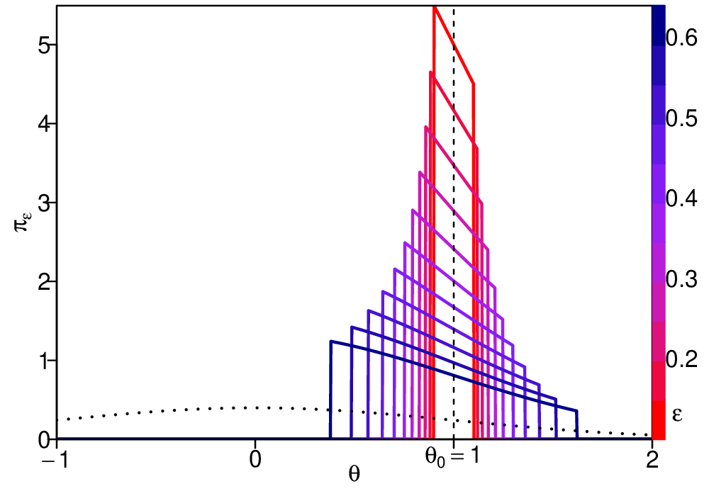
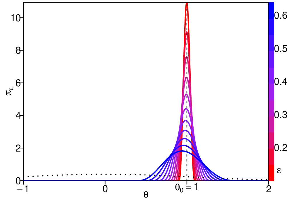
where we write from now on and as for the Lebesgue measure. To make the conclusions of Theorem 2, we require a choice of that satisfies B4. Two possibilities are the venerable accept/reject kernel and the triweight kernel which corresponds to a choice of and . In either case, since , it is then procedural to verify the remaining assumptions B1–B3 of Theorem 2, which then implies that the pseudo-posterior and coarsened posterior can be made to concentrate on sets of arbitrarily small Lebesgue measure by making sufficiently small. We visualize the concentration of the limiting measure in Figure 1, for both the cases of the accept/reject and triweight kernels. Observe that the masses of both limiting measures concentrate on smaller intervals around as decreases, as expected from our theory. The choice of weight functions influences the smoothness and shape of the posterior densities but does not affect the size of the support.
Remark 5.
Besides our choices for , one can use any common kernel with compact support from the theory of density estimation, such as the triangular or Epanechnikov kernels (cf. Scott 2015, Ch. 6).
6.2 Finitely unidentifiable normal model
We now instead suppose that is an IID sequence defined by for each , and that is independent of , with elements , where . We again use the distance (5), which P-a.s. converges to .
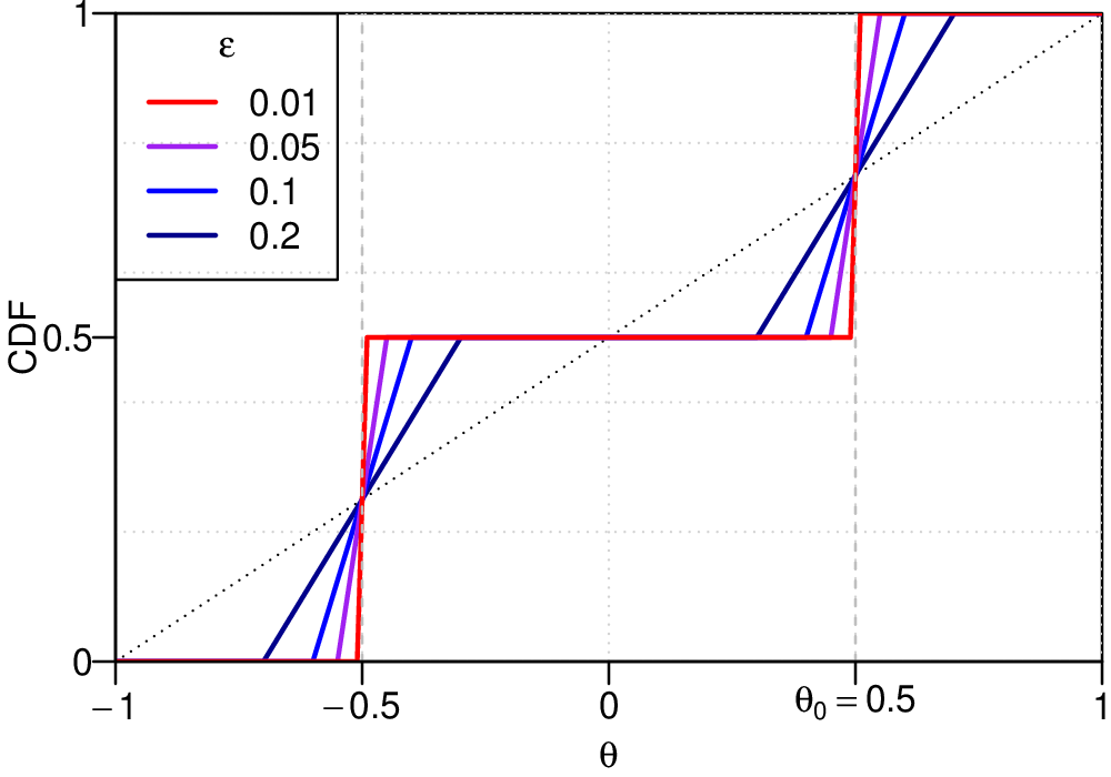
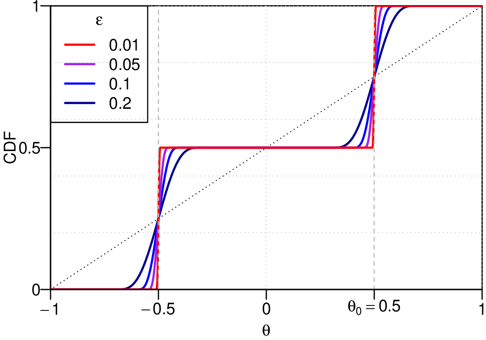
For non-zero generative parameter , B1 holds with . B2 holds since implies that . The verification of the remaining assumptions A1–A3 and B3–B4 for the case of set to the accept/reject and triweight kernels follows from analogous arguments to those made in Section 6.1. As such, we have the fact that the pseudo-posterior and coarsened posterior measures concentrate mass on sets with arbitrarily small Lebesgue measure, for sufficiently small , and have limiting densities
| (9) |
and
| (10) |
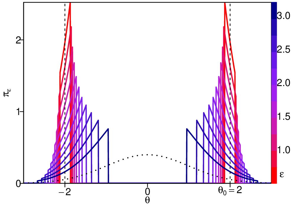
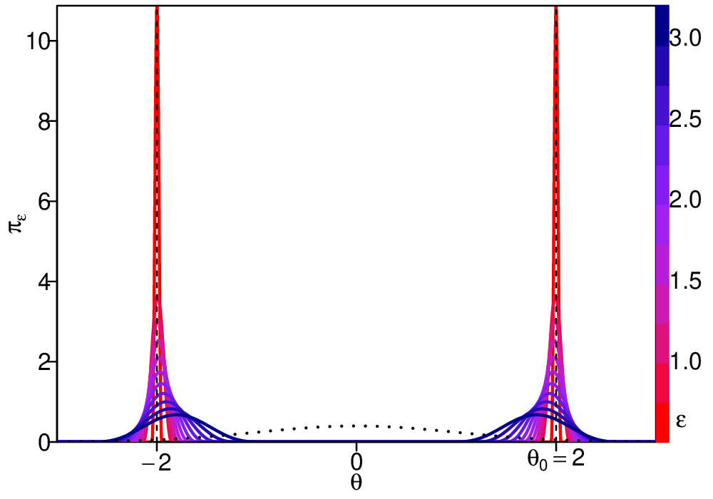
when is taken as either the accept/reject or triweight kernels, respectively. We plot the concentration of mass of the corresponding measures for various values of in Figure 2. Unlike Figure 1, we observe that the limiting posterior distributions not only concentrate mass around but also around , since is the same in both cases. As predicted by our theory, as decreases, the limiting distributions are supported on smaller sets containing and , which are independent of the choice of weights.
6.3 Infinitely unidentifiable normal model
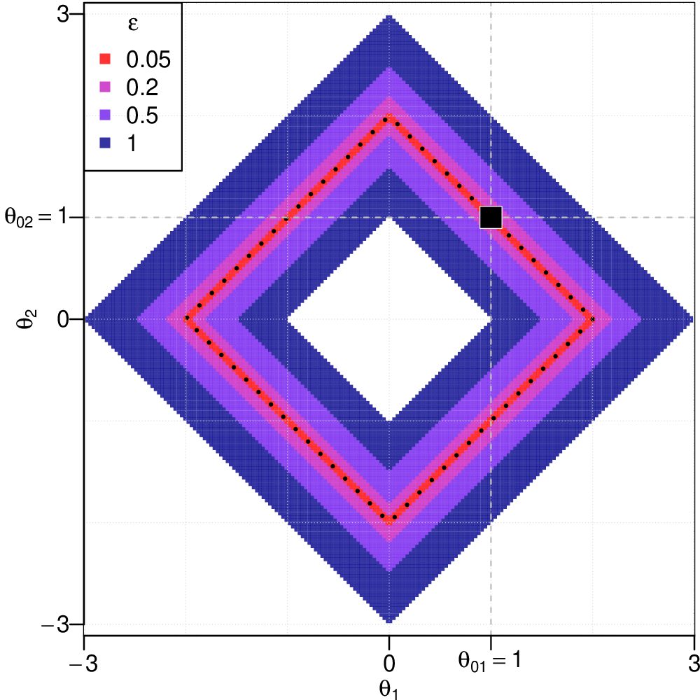
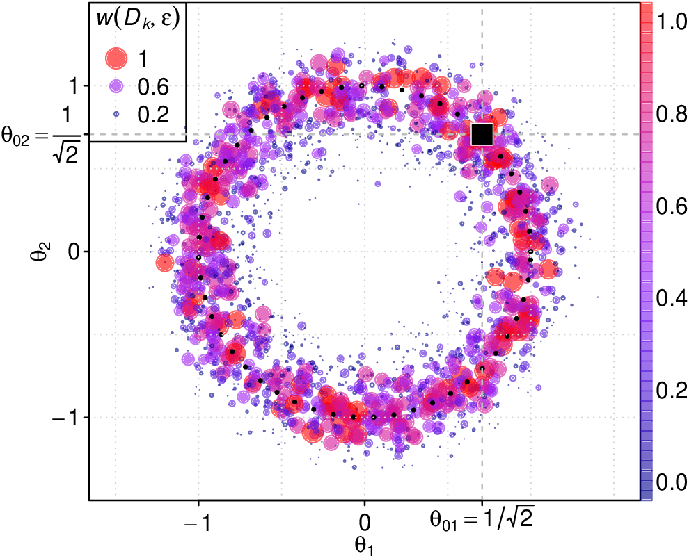
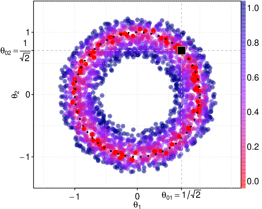
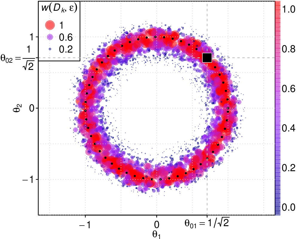
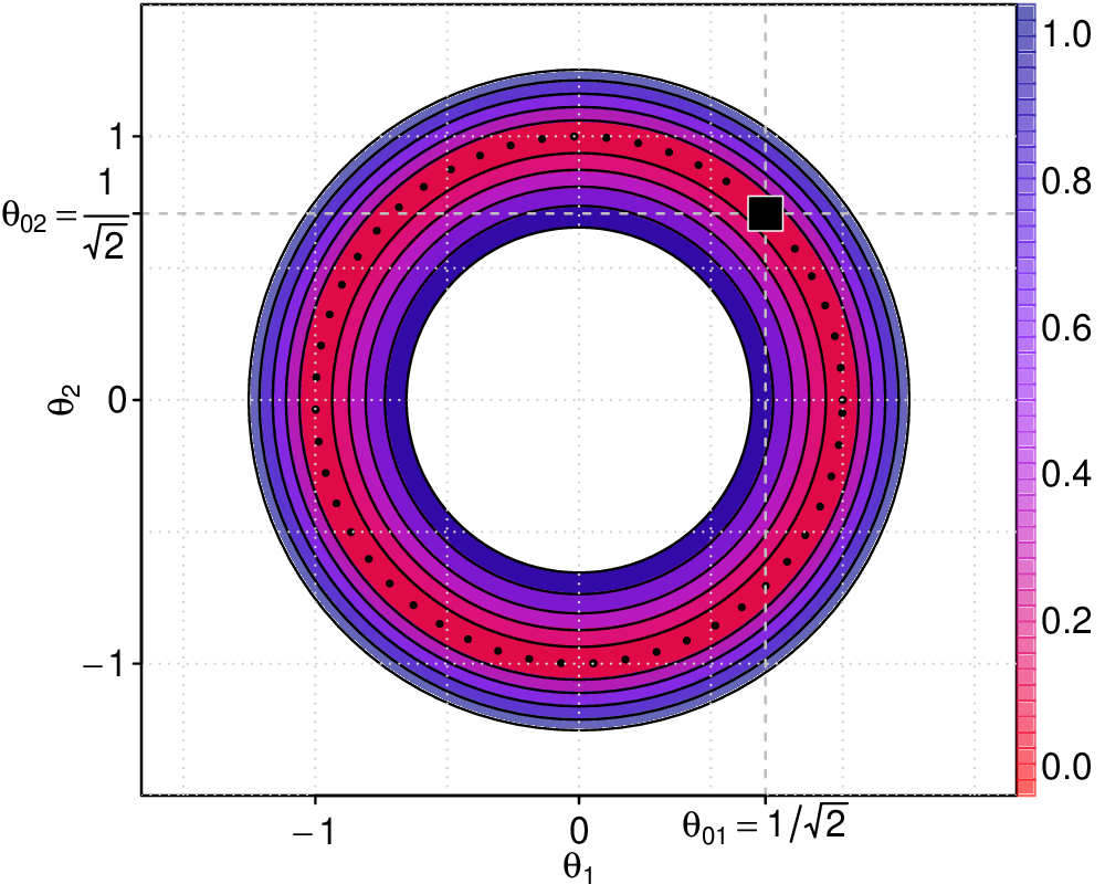
We further complicate the situation by supposing that is an IID sequence defined by for each , and that is independent of , with IID elements . In this example, and are elements in with and denoting their L1-norms. We use the prior and consider the distance (5), which P-a.s. converges to . B1 holds with and B2 holds with since implies that and for each . We also have to verify B3, which can be achieved by noting that is the contour of the -ball of radius and thus consists of four line segments, each of length , where . We can cover each of line segments with Euclidean balls of radius by placing a ball on each of the equidistant points along the line, of distance apart. Then, we can check B3 by evaluating , which approaches zero as , as required. The verification of A1–A3 and B4 for concluding Theorem 1 Part (i) and Theorem 2 Part (ii) using set to the accept/reject and triweight kernels is then procedural. We illustrate the concentration of mass by plotting the support of the limit (8) of both of the ABC posterior densities, defined by (6) and (7), in Figure 3. For both kernels, the support satisfies or equivalently , which corresponds to the region between the L1-balls of radii and .
Remark 6.
We have used the example of normal distributions for the measures of (), and , in all of the examples above out of convenience. Of course, the same illustrations can be made if we replace all uses of the normal law , with density , by any generic location-scale law defined by density with location and scale parameters and , provided that the necessary integrals with respect to exist.
7 Numerical estimation of posterior measures
We have opted for examples with summary-based discrepancy functions and for IID sequences and , for ease of understanding and simplicity of exposition. However, the main conclusions of Proposition 1 and Theorem 1 apply in much broader settings, as we will demonstrate below.
7.1 Non-IID sequences from a first-order autoregressive model
In this example, we consider , where can be characterized as
where , , and is IID with . Similarly, we write , characterized by , with , where and is IID with . We shall use a uniform prior density . Via Hall and Heyde (1980, Thm. 6.6), we have the following strongly consistent estimators of and from and : and , respectively. Thus, the distance converges, P-a.s., to .
To estimate the ABC posterior measures, we sample and compute as described in Algorithm 1. For any given , we can then characterize the ABC posterior measures via their cumulative distribution functions (CDFs), estimated by the respective empirical CDFs. The larger the value of , the more accurate the empirical distribution is to its target. When we take to be the accept/reject kernel, the empirical CDF is given by:
| (11) |
In the same way, when taking to be the triweight kernel, we can estimate CDFs that characterize the ABC posterior measures, for any given , via the empirical weighted CDF:
| (12) |
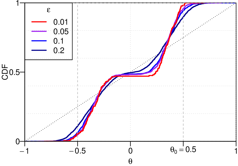
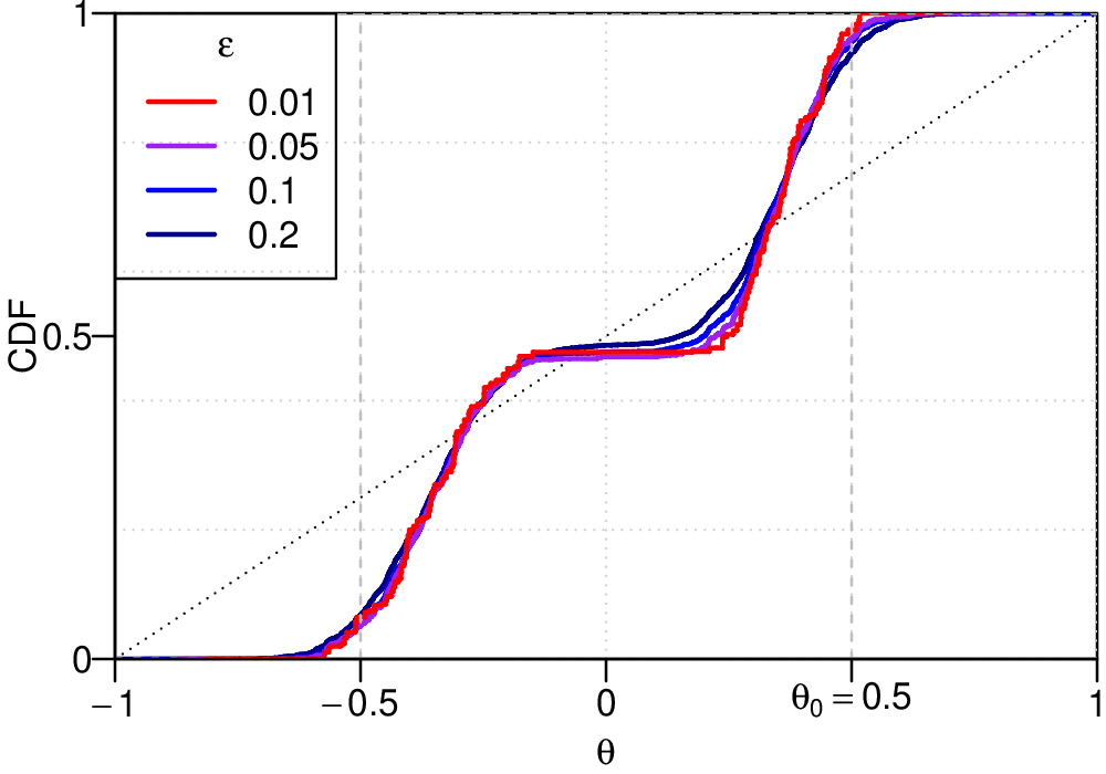
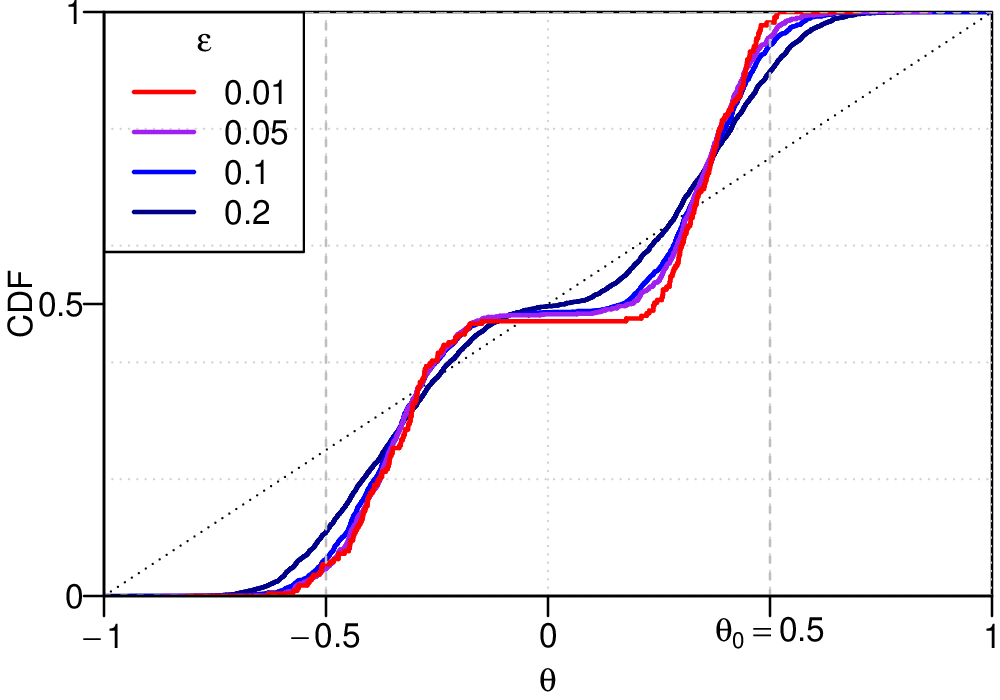
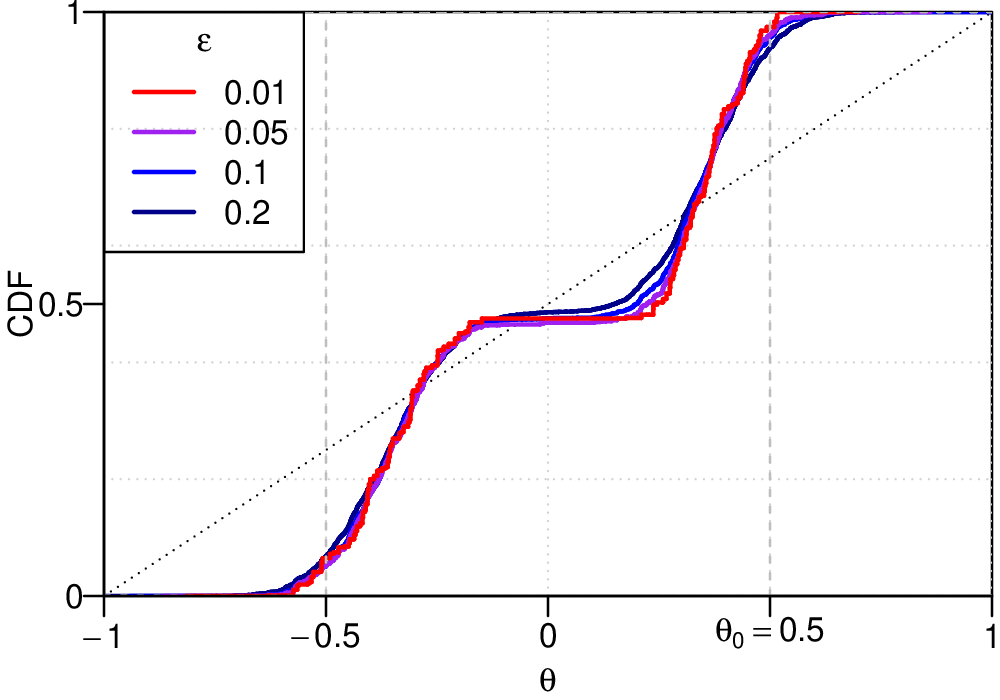
Figure 4 displays sample functions (11) and (12) from an experiment with , , and . We observe that the empirical cumulative distribution functions both concentrate around the estimates , which converge towards the zeroes of : . The support of the sample measures are supersets of the estimates that decrease in size as decreases towards zero, as expected. We also observe that, for fixed , the empirical cumulative distribution functions both converge to their limiting forms, as increases, as predicted by Remark 2.
Input: Data , discrepancy function , number of Monte Carlo replications .
For :
Sample from a measure with density ;
Generate from a measure with density ;
Compute discrepancy .
Output: Discrepancies ; Parameters .
| (a) | |
 |
 |
| (b) | |
 |
 |
| (c) | |
 |
 |
7.2 Wasserstein distance in Gaussian model
For this example, we take to be an IID sequence of random variables, where , for each . We let and endow with the prior measure defined by the uniform density . We then take to be an IID sequence, independent of , such that , for each .
To measure the distance between partial sequences and , we use the sample -Wasserstein distance
where and are the order statistics of and , respectively (cf. Peyré and Cuturi 2019, Rem. 2.28). In this case, the -Wasserstein distance between measures on is just the distance between the distribution functions of and , and (Peyré and Cuturi, 2019, Rem. 2.30). The Glivenko–Cantelli theorem implies that converges P-a.s. to . To verify B2, we use the fact that the 1-Wasserstein distance between normal distributions and is , for (cf. Chafai and Malrieu, 2010, Example. 2.5).
We use Algorithm 1 to obtain samples and discrepancies to estimate the ABC posteriors using the accept/reject kernel and the triweight kernel in place of . Simulations are carried out with , , and . Interpreting the expression as meaning and (for ), we provide representations of the obtained estimated empirical distribution functions of form (11) and (12) via their weighted point masses in Figure 5, along with an illustration of the supports of the limiting ABC posterior measures for various values of . We observe, as predicted, that the estimated ABC posterior measures concentrate on supersets of the zeroes of , which can be characterized by the contour of the L2-ball of radius : , where the sets get smaller in volume as decreases, and where smaller weights are assigned for larger deviations from . As expected from Remark 2, we observe that the supports of the empirical representations converge to those of the limiting measures, as increases, for fixed values of .
Note that, when and arise from general location-scale distributions instead of normal distributions, we can use the formula of Gelbrich (1990, Cor. 2.4) with the Wasserstein norm equivalence result of Garling (2018, Cor. 21.2.4) to verify B2.
| (a1) , varies | (a2) , weights representation |
|---|---|
 |
 |
| (b1) , varies | (b2) , weights representation |
 |
 |
| (c) , varies | |
 |
8 Application to binaural sound source localization
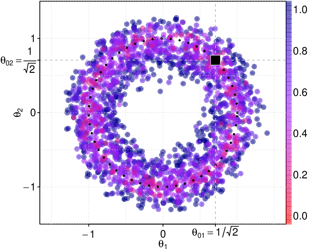
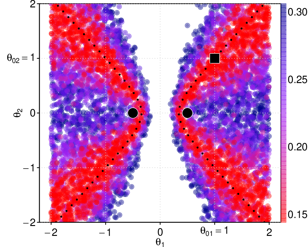
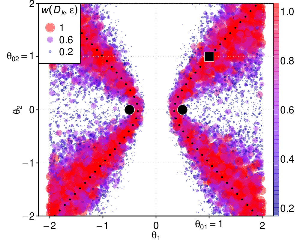
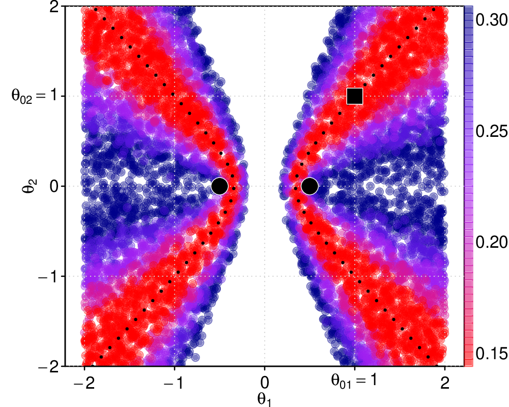
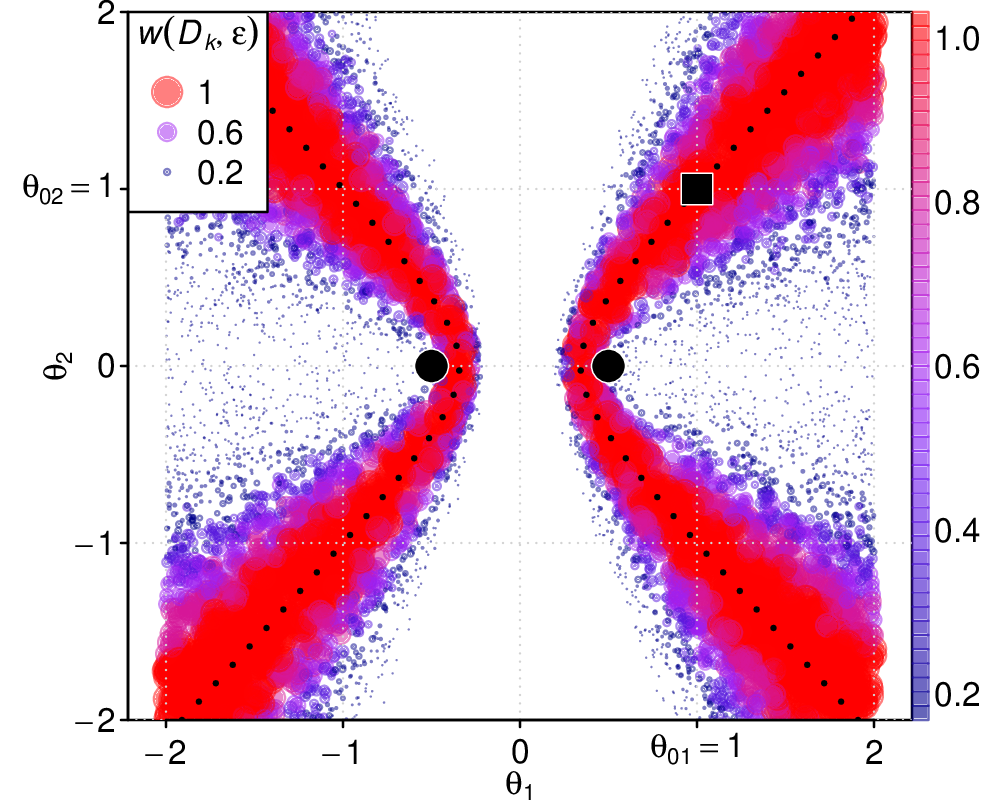
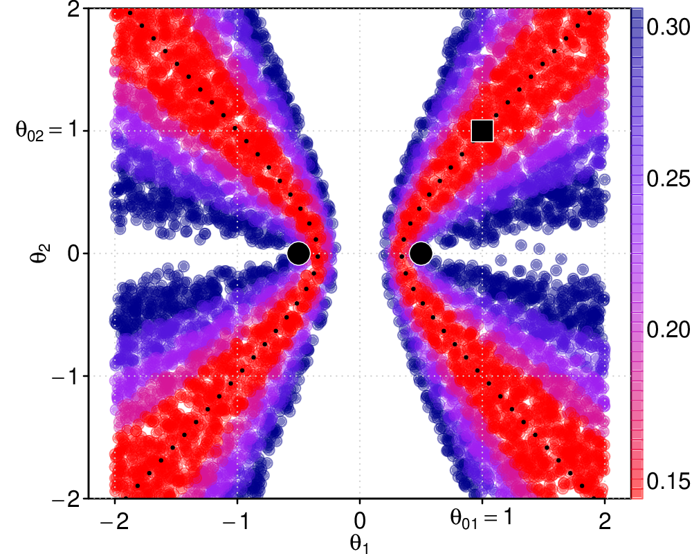
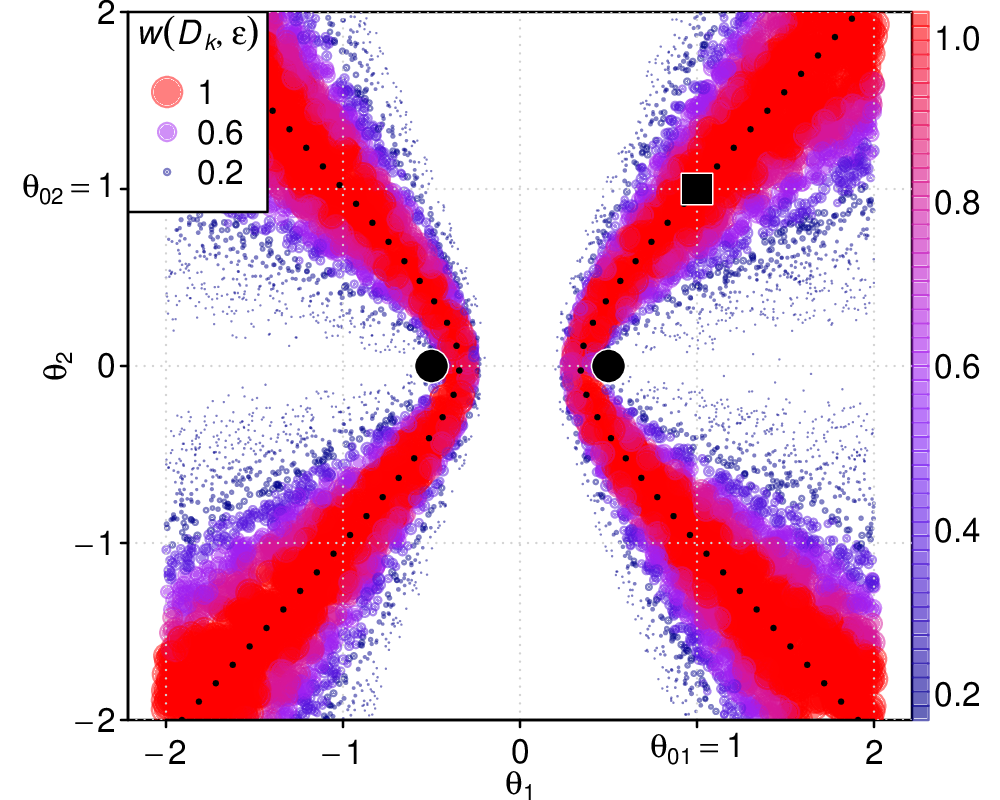
The following example is a simplified version of a synthetic example of Forbes et al. (2022) related to sound source localization. Here, we take to be an IID sequence of random variables, with , for each , and is interpreted as the 2D position of a sound source, assumed to be captured only through the noisy measurements of so-called interaural time differences (ITDs). In a binaural setting with two microphones, the ITD is defined as the difference between the time of arrival to the first and second microphone and given by for a source in and microphones at positions . ITD measurements only allow us to determine a pair of hyperbolas on which the source may be. We let and endow with the prior measure defined by the uniform density . We then take to be an IID sequence, independent of , such that , for each .
We proceed in the same manner as in Section 7.2. That is, to measure the distance between partial sequences and , we use the -Wasserstein distance , where and are the order statistics of and , respectively. Again, the -Wasserstein distance between measures on is just the distance between the distribution functions of and , and , and we have the convergence of , P-a.s., to , with B2 verified via the form of the 1-Wasserstein distance: (cf. Chafai and Malrieu, 2010, Example. 2.5).
We again use Algorithm 1 to obtain prior and discrepancy samples to estimate the ABC posteriors using the accept/reject kernel and the triweight kernel in place of . Simulations are carried out with , , and . We provide representations of the obtained estimated empirical distribution functions via their weighted point masses in Figure 6. We observe, as predicted, that the estimated ABC posterior measures concentrate on supersets of the zeroes of which consists of two hyperbolas as shown in Figure 6. Observe that smaller values of correspond to sets with elements that sit closer to the zeroes of . We also observe that smaller weights are assigned for larger deviations from the zeroes of .
| (a1) , varies | (a2) , weights representation |
 |
 |
| (b1) , varies | (b2) , weights representation |
 |
 |
| (c1) , varies | (c2) , weights representation |
 |
 |
9 Conclusion and future directions
In summary, we have provided a set of results that permit the establishment of posterior quasi-consistency of ABC posterior measures in the and almost sure sense, in scenarios that lack identifiability, when discrepancies are possibly not Hölder continuous, and when the sequences and are potentially non-IID. Our results complement the existing literature and deliver theoretical guarantees to situations that are not covered by previous works.
Our contributions suggest several potential directions for further research. Open questions include whether our approach can be extended to prove the concentration of ABC posterior measures when the weight function is supported on an unbounded domain, whether this approach can prove concentration results in the setting, and whether our proof techniques can be extended to provide approximation and estimation rates that either improve upon those proposed by others, such as Frazier et al. (2018), Bernton et al. (2019), and Legramanti et al. (2025), or relax the assumptions that are previously made. We aim to address these questions in our future work.
Acknowledgments
All authors acknowledge funding from the Australian Research Council grant number DP230100905, and from Inria Project WOMBAT.
Appendix A Technical results
Lemma 2 (Hunt’s Lemma).
Let be a probability space and be a filtration on . Further, define . Let , , and be random variables mapping from , such that , where , -a.s., for each , such that . Then, , -a.s., and in .
Appendix B Proofs of main results
B.1 Proof of Proposition 1
We use the canonical representation of that supports the definitions of and . That is, we write with typical elements , and equip it with its Borel -algebra . We then, define , with typical element , and equip it with the -algebra . For each , write and . For each , we characterize the measure on via the density function
| (13) |
with respect to the dominating measure , and we assume that is a consistent sequence in the sense of the Ionescu–Tulcea extension theorem. We shall write to denote the unique measure on that is compatible with the measures defined by (13).
Further, for each and -a.a. , we define the conditional distribution of given by as the measure defined by
and denote the compatible conditional measure on by . Let be a filtration, where , and write to be its limit.
Next, we set
By A2, we can set , so that . By A1, we have
| (14) |
for -a.a. . Then, by A3, we can apply the continuous mapping:
Using the filtration , we then apply Lemma 2, which implies that
and
for -a.a. . By definition of , we have
and since
for -a.a. , we conclude that, for -a.a. ,
| (15) |
and
| (16) |
B.2 Proof of Lemma 1
Let us define the Minkowski sum of sets as . By B3, we have -covering centres of (as defined by B1 and B2). This then implies that . By the monotonicity of Minkoswki addition, , where we use the fact that if is convex, then (cf. Schneider 2013, Ch. 3). Now, using the fact that the Lebesgue measure of is and by monotonicity, we obtain the fact that
since .
B.3 Proof of Theorem 1
Notice first that for each , has support , by B4. But by B1 and B2, for each , there exists a , such that if , then , and thus
and
where the equality holds by the fact that is zero when . Thus,
since . Here, by appropriately choosing , we can make as small as we like via Lemma 1. Under A1–A3, we obtain the conclusion from Remark 2, implying that converges in total variation to , P-a.s., and converges in total variation to . But by definition of convergence in total variation, we must also have the set-wise convergence statements and , for any (cf. Hernández-Lerma and Lasserre, 2003, Sec. 1.4.2). Thus,
and
as required.
References
- Approximate bayesian computation in population genetics. Genetics 162 (4), pp. 2025–2035. Cited by: §3. ↩ 3
- Approximate Bayesian computation. Annual Review of Statistics and its Application 6, pp. 379–403. Cited by: §1. ↩ 1
- Approximate Bayesian computation with the Wasserstein distance. Journal of the Royal Statistical Society: Series B (Statistical Methodology) 81 (2), pp. 235–269. Cited by: item, item, Table 1, §2, §2, §2, §9, Remark 4. ↩ 1 2 5 9
- On fine properties of mixtures with respect to concentration of measure and Sobolev type inequalities. Annales de l’IHP Probabilités et Statistiques 46, pp. 72–96. Cited by: §7.2, §8. ↩ 7.2 8
- Probabilities and potential, b: theory of martingales. Elsevier. Cited by: Remark 7. ↩ A
- Summary statistics and discrepancy measures for approximate Bayesian computation via surrogate posteriors. Statistics and Computing 32. Cited by: §4, §8. ↩ 4 8
- Asymptotic properties of approximate Bayesian computation. Biometrika 105 (3), pp. 593–607. Cited by: Table 1, §2, §2, §2, §9. ↩ 1 2 9
- Model misspecification in approximate Bayesian computation: consequences and diagnostics. Journal of the Royal Statistical Society: Series B (Statistical Methodology) 82 (2), pp. 421–444. Cited by: Table 1, §2, §2, Remark 4. ↩ 1 2 5
- Analysis on polish spaces and an introduction to optimal transportation. Cambridge University Press. Cited by: §7.2. ↩ 7.2
- On a formula for the L2 Wasserstein metric between measures on Euclidean and Hilbert spaces. Mathematische Nachrichten 147 (1), pp. 185–203. Cited by: §7.2. ↩ 7.2
- Fundamentals of nonparametric bayesian inference. Vol. 44, Cambridge University Press. Cited by: §5. ↩ 5
- Martingale limit theory and its application. Academic Press. Cited by: §7.1. ↩ 7.1
- Markov chains and invariant probabilities. Birkhauser. Cited by: §B.3. ↩ B.3
- Approximate Bayesian computation with Kullback-Leibler divergence as data discrepancy. In International Conference on Artificial Intelligence and Statistics, pp. 1711–1721. Cited by: §1, Table 1, §2, §4, Remark 1. ↩ 1 2 4
- An approximate likelihood perspective on ABC methods. Statistics Surveys 12, pp. 66–104. Cited by: §1, §3. ↩ 1 3
- Concentration of discrepancy-based approximate Bayesian computation via Rademacher complexity. Annals of Statistics 53 (1), pp. 37 – 60. External Links: Document Cited by: Table 1, §2, §2, §2, §9, Remark 4. ↩ 1 2 5 9
- Convergence of regression-adjusted approximate Bayesian computation. Biometrika 105 (2), pp. 301–318. Cited by: §1, Table 1, §2, §2, §3. ↩ 1 2 3
- On the asymptotic efficiency of approximate Bayesian computation estimators. Biometrika 105 (2), pp. 285–299. Cited by: §1, Table 1, §2, §2, §3. ↩ 1 2 3
- Real Analysis: Measures, Integrals and Applications. Springer, New York. Cited by: §4. ↩ 4
- Approximate Bayesian computational methods. Statistics and Computing 22 (6), pp. 1167–1180. Cited by: §1, §1, §3, §4. ↩ 1 3 4
- Robust Bayesian inference via coarsening. Journal of the American Statistical Association 114 (527), pp. 1113–1125. Cited by: §1, §1, Table 1, §2, §3, Remark 1. ↩ 1 2 3 4
- Approximate Bayesian computation via the energy statistic. IEEE Access 8, pp. 131683–131698. Cited by: §1, §1, Table 1, §2, §3, §4, §5, Remark 1. ↩ 1 2 3 4 5
- K2-ABC: Approximate Bayesian computation with kernel embeddings. In Artificial Intelligence and Statistics, pp. 398–407. Cited by: §1, §3, §5. ↩ 1 3 5
- Computational optimal transport: with applications to data science. Foundations and Trends in Machine Learning 11 (5-6), pp. 355–607. Cited by: §7.2. ↩ 7.2
- General Topology. An Introduction, De Gruyter. External Links: ISBN 978-3-11-068657-9, Document Cited by: §5. ↩ 5
- A simple approach to maximum intractable likelihood estimation. Electronic Journal of Statistics 7, pp. 1632–1654. Cited by: item, Table 1. ↩ 1
- Convex Bodies: The Brunn–Minkowski Theory. 2 edition, Encyclopedia of Mathematics and its Applications, Cambridge University Press, Cambridge. External Links: ISBN 978-1-107-60101-7, Document Cited by: §B.2. ↩ B.2
- Multivariate density estimation: theory, practice, and visualization. John Wiley & Sons. Cited by: §3, Remark 5. ↩ 3 6.1
- Handbook of approximate bayesian computation. CRC Press. Cited by: §1. ↩ 1
- Analysis and probability. Elsevier, Oxford. Cited by: §3, Remark 7. ↩ 3 A
- Approximate bayesian computation (ABC) gives exact results under the assumption of model error. Statistical Applications in Genetics and Molecular Biology 12, pp. 129–141. Cited by: §3. ↩ 3