Bayesian nonparametric mixture of experts for inverse problems

TrungTin Nguyen; Florence Forbes; Julyan Arbel; Hien Duy Nguyen

Abstract

Large classes of problems can be formulated as inverse problems, where the goal is to find parameter values that best explain some observed measures. The relationship between parameters and observations is typically highly non-linear, with relatively high dimensional observations and correlated multidimensional parameters. To deal with these constraints via inverse regression strategies, we consider the Gaussian Local Linear Mapping (GLLiM) model, a special instance of mixture of expert models. We propose a general scheme to design a Bayesian nonparametric GLLiM model to avoid any commitment to an arbitrary number of experts. A tractable estimation algorithm is designed using variational Bayesian expectation-maximisation. We establish posterior consistency for the number of mixture components after the merge-truncate-merge algorithm post-processing. Illustrations on simulated data show good results in terms of recovering the true number of experts and the regression function.

Keywords: B

ayesian nonparametrics; mixture of experts; inverse problems; Gaussian locally-linear mapping models; linear cluster-weighted models; variational inference; clustering; regression; model selection.

1 Introduction

Inverse problems.

Many problems can be formulated as inverse problems, where the goal is to find parameter values that best explain an observed phenomenon. Typical constraints in practice are that the relationships between parameters and observations are highly non-linear, with relatively high dimensional observations and correlated multivariate parameters. To handle these constraints, we consider probabilistic mixtures of locally linear models, namely the Gaussian locally linear mapping (GLLiM) approach of Deleforge et al. (2015), which includes affine instances of the mixture of experts (MoE) model (Xu et al., 1995) and the classical inverse linear regression model (Hoadley, 1970; Li, 1991), as special cases. We propose to address inverse problems in a Bayesian framework, making use of the availability of simulations from forward models of interest. The GLLiM approach has been used in many applications, e.g., in medical imaging (Boux et al., 2021), planetary science (Kugler et al., 2022; Nguyen et al., 2024a), head-pose estimation problem in computer vision (Lathuilière et al., 2017) and quantitative trait prediction from biological data (Blein-Nicolas et al., 2024).

Mixture of experts models (MoE)

are generalizations of neural network architectures proposed by Jacobs et al. (1991). Further, these flexible models also generalize the classical mixture models (MMs) and mixture of regression models (McLachlan and Peel, 2000). Their flexibility comes from the fact that they allow the mixture weights (or the gating functions) to depend on the explanatory variables, together with the component densities (or the experts). In regression, MoE models with Gaussian experts and softmax or normalized Gaussian gating functions (as in GLLiM) are the most popular choices. These models are powerful tools for modelling complex nonlinear relationships between outputs (responses) and inputs (predictors) that arise from different subpopulations. The popularity of these conditional mixture density models is largely due to their universal approximation properties (Norets, 2010; Nguyen et al., 2016, 2019, 2021a) as well as their good convergence rate, see, e.g., for mixture of regression in Ho et al. (2022) and for MoE in Jiang and Tanner (1999); Nguyen et al. (2024c, 2023a, b). It is worth noting that these results improve the approximation capabilities and convergence rates of unconditional MMs, as discussed in Genovese and Wasserman (2000); Rakhlin et al. (2005); Nguyen (2013); Shen et al. (2013); Ho and Nguyen (2016a, b); Nguyen et al. (2020, 2023b). At a high level, universal approximation theorems state that given a large enough number of components, MMs and MoE models can approximate a large class of unconditional and conditional probability density functions (cPDF), respectively, to any degree of accuracy. See, e.g., Yuksel et al. (2012); Nguyen and Chamroukhi (2018); Do et al. (2023); Nguyen (2021); Chen et al. (2022), for further detailed reviews of practical and theoretical aspects of MoE models in statistics and in diverse domains, e.g., natural language processing and computer vision.

Model selection in MoE models.

Although universal approximation allows us to conclude that, given a sufficient number of components, a finite MoE can approximate any other cPDF to an arbitrary degree of accuracy, it is not clear how to choose a large enough number of components for realistic problems. This motivates a careful study of interesting and important model selection problems for MMs and MoE models, which have attracted much attention in statistics and machine learning over the last 50 years, see, e.g., Celeux et al. (2019); Gormley and Frühwirth-Schnatter (2019) for a recent comprehensive review.

When selecting the best data-driven number of components for MoE models, there are several approaches to controlling and accounting for model complexity. Typically, model selection in MoE models is performed using an information criterion, such as the Akaike information criterion (AIC; Akaike, 1974; Frühwirth-Schnatter et al., 2018), the Bayesian information criterion (BIC; Schwarz, 1978; Berrettini et al., 2024, BIC-GLLiM; Forbes et al., 2022a, b), the BIC-like approximation of integrated classification likelihood (ICL-BIC; Biernacki et al., 2000; Frühwirth-Schnatter et al., 2012), extended BIC for mixture Gaussian graphical models (eBIC; Nguyen and Li, 2024; Foygel and Drton, 2010), or Sin and White information criterion (SWIC; Sin and White, 1996; Westerhout et al., 2024) for stationary sequences that are not independently and identically distributed. However, an important limitation of these criteria is that they are only asymptotically valid. This means that there are no finite sample guarantees when using AIC, BIC, ICL-BIC or SWIC to choose between different levels of complexity. Therefore, their use in small sample settings is ad hoc.

To overcome such difficulties, and to partially support the so-called slope heuristic approach (Birgé and Massart, 2007, also see Arlot, 2019 for a recent review), Nguyen et al. (2021b, 2022c, 2022b, 2023d, 2023c) recently established non-asymptotic risk bounds in the form of weak oracle inequalities, provided that lower bounds on the penalties hold, in high-dimensional regression scenarios for a variety of MoE models, including GLLiM. Another approach, as proposed by Nguyen et al. (2022a), is based on the closed testing principle, which leads to a sequential testing procedure that enables confidence statements regarding the order of a finite mixture model. These methods facilitate an optimal data-driven selection of the number of components in finite-sample settings. Additionally, Bayesian model selection, which employs marginal likelihoods as a criterion, provides another strategy for determining the number of components in MoE models (Frühwirth-Schnatter, 2019; Zens, 2019). However, all previous approaches require that a range of models with different values be trained and compared, which can be a computational bottleneck in a high-dimensional framework.

Recently, Kock et al. (2022) proposed computationally efficient variational inference approaches for architecture selection in high-dimensional deep Gaussian mixture models using overfitted mixtures (see, e.g., Rousseau and Mengersen, 2011; Forbes et al., 2019), where unnecessary components are dropped in the estimation. The same idea is applied in the context of overfitting sparse Bayesian factor analysis in Frühwirth-Schnatter et al. (2024), where the authors employed the Markov Chain Monte Carlo (MCMC) procedure, followed by post-processing of posterior draws, to facilitate practical Bayesian inference. However, we are interested here in the more general context of the Bayesian nonparametric (BNP) approach, (see, e.g., Hjort et al., 2010; Ghosal and Van der Vaart, 2017), where it is not necessary to know an upper bound of the true number of components as in Bayesian overfitted MM. This is one motivation for the BNP priors that are considered here for GLLiM.

Dirichlet process mixture models (DP-MMs) and Pitman-Yor process mixture models (PYP-MMs) are among the most popular BNP models, particularly suitable for density estimation and probabilistic clustering. However, the posterior of the DP-MMs or PYP-MMs are inconsistent for the number of components if the true number of components is finite and the concentration parameter is fixed (see, e.g., Miller and Harrison, 2014, and Alamichel et al., 2024 for a review). This is because a BNP prior such as DP or PYP places zero probability on mixing measures with a finite number of supporting atoms. An interesting recent result in Ascolani et al. (2022) is that consistency for the number of components can be achieved if a prior is placed on the concentration parameter of the DP-MM, under some assumptions on this prior.

It appears that BNP-GLLiM tends to produce many small extraneous components around the true clusters in our numerical experiment Section 6. This makes it difficult to use them to infer the true number of components when this becomes a quantity of interest (Maceachern and Müller, 1998; Green and Richardson, 2001). This encourages the use of a novel, simple post-processing algorithm in the spirit of the Merge-Truncate-Merge (MTM) introduced by Guha et al. (2021). This post-processing procedure consistently estimates the number of components for any general Bayesian prior, even without knowing its exact structure, as long as the posterior for that prior contracts to the true mixing distribution at a known rate.

Contributions.

To address the challenges of highly nonlinear inverse problems with relatively high dimensional observations and correlated parameters, we propose a novel BNP-GLLiM model and inference procedure, which is computationally efficient and avoids any commitment to an arbitrary number of components. Although BNP mixture models (BNP-MM), which are special cases of the BNP-GLLiM model, have been extensively studied in the literature (Escobar and West, 1995; Maceachern and Müller, 1998; Neal, 2000; Arbel et al., 2021; Li et al., 2022; Durand et al., 2022), the extension to MoE models in an inverse regression framework has not been covered. In addition, we establish theoretical properties such as posterior consistency for recovering the true number of components in BNP-GLLiM using the post-processing merge-truncate-merge (MTM) algorithm. Finally, our illustrations on simulated data show good results in terms of recovering the true number of components and mean regression functions. It is worth emphasising that, for the first time, we provide evidence that MTM consistency holds not only for the MMs results of Guha et al. (2021), but also in the more general context of MoE models for cPDFs.

Notations.

Throughout this paper, ${1, \dots, D}$ is abbreviated as $[D]$ for $D \in ℕ^{⋆}$ , where $ℕ^{⋆}$ denotes the positive natural numbers. The notation $\equiv$ refers to a definition. It is used to simplify the notation or expression. For a parametric model $S$ , $dim (S)$ refers to its dimension, i.e., the total number of parameters to be estimated. Furthermore, $[\cdot; \cdot]$ denotes vertical vector concatenation. Throughout, we use the following colour rule for observations and parameters: observations are represented in green; latent, random or unknown parameters in red; and (fixed) hyperparameters in blue.

Outline.

The paper is organized as follows. In Section 2, we first discuss how to construct the BNP-GLLiM model. A VBEM algorithm and the corresponding ELBO are described in Section 3, and predictive cPDFs in Section 4. Next, Section 5 shows how we can integrate the Merge-Truncate-Merge (MTM) post-processing procedure and prove consistency for the MTM output. This is useful to perform regression, clustering and model selection, simultaneously. We experimentally evaluate our new results on simulated datasets in Section 6. Some perspectives are provided in Section 7. We recall the standard Bayesian nonparametric priors and variational Bayesian expectation-maximisation principle in Appendices A and B, respectively. All details of VBEM for the BNP-GLLiM model, evidence lower-bound, and technical proofs not included in the main paper are relegated to Appendices C, D and E, respectively. Appendix F presents a more general model with a hyperprior on the gating parameters, called BNP-GLLiM2.

2 BNP-GLLiM model

In Sections 2.1 and 2.2, we present the advantage of adopting a GLLiM model, which uses an inverse regression approach to estimate nonlinear high-to-low dimensional mappings. Such a strategy allows to greatly reduce the number of required parameters. To avoid any commitment to an arbitrary number of components, we then construct the BNP-GLLiM model in Section 2.3.

2.1 Inverse regression framework

We are interested in estimating the law of a low-dimensional random variable $𝐗 = (𝐗_{l})_{l \in [L]}$ conditionally on a high-dimensional $𝐘 = (𝐘_{d})_{d \in [D]}$ , where typically $D ≫ L$ . We follow an inverse regression framework as in e.g., Li (1991); Deleforge et al. (2015). Therefore, in training, the low-dimensional variable $𝐗$ plays the role of the regressor, while the response $𝐘$ is a function of $𝐗$ , possibly corrupted by noise through inverse cPDF $p (𝐘 ∣ 𝐗; 𝝍$ ), where $𝝍$ is an inverse parameter. The low dimension of the regressor $𝐗$ allows to drastically reduce the number of parameters to be estimated. In addition, the forward parameter $𝝍^{*}$ and cPDF $p (𝐗 ∣ 𝐘; 𝝍^{*})$ are tractable after estimating the inverse parameter $𝝍$ . Therefore, this density can be used to predict the low-dimensional response $𝐱$ of a high-dimensional test point $𝐲$ . This inverse-then-forward regression strategy justifies the unconventional notation: $𝐘$ for the high-dimensional input and $𝐗$ for the low-dimensional response. Here and subsequently, we refer to the low-dimensional data sample as $𝒳 \equiv {𝐱_{n}}_{n \in [N]} \subset (ℝ^{L})^{N}$ , the high-dimensional data sample as $𝒴 \equiv {𝐲_{n}}_{n \in [N]} \subset (ℝ^{D})^{N}$ . We denote the observed values as $(𝐱, 𝐲)$ , which are independently and identically distributed (i.i.d.) samples from the random variables $(𝐗, 𝐘)$ .

2.2 Nonlinear high-to-low dimensional mapping via GLLiM model

The GLLiM models, as originally introduced in Deleforge et al. (2015), are used to capture the non-linear relationship between the response and the set of covariates from a high-to-low heterogeneous data. Specifically, Deleforge et al. (2015) overcame the difficulty of high-to-low regression by tackling the problem the other way round, i.e., low-to-high. This means that the roles of input and response variables are swapped so that the low-dimensional variable $𝐗$ becomes the regressor as in Section 2.1. GLLiM then relies on a piecewise linear model in the following way. The high-dimensional response $𝐘$ is approximated by the local affine mappings $K$ :

𝐘 = \sum_{k = 1}^{K} 𝕀 (Z = k) (𝐀_{k} 𝐗 + 𝐛_{k} + 𝐄_{k}) .

Here, $𝕀$ is an indicator function and $Z$ is a latent variable that captures a cluster relationship, such that $Z = k$ if $𝐘$ comes from cluster $k \in [K]$ . Matrices $𝐀_{k} \in ℝ^{D \times L}$ and vectors $𝐛_{k} \in ℝ^{D}$ define cluster-specific affine transformations. In addition, $𝐄_{k}$ are error terms that capture both the reconstruction error due to the local affine approximations as well as the observation noise in $ℝ^{D}$ .

Following the usual assumption that $𝐄_{k}$ is a zero-mean Gaussian variable with a covariance matrix $𝚺_{k} \in ℝ^{D \times D}$ , it follows that

p (𝐲 ∣ 𝐱, Z = k; 𝝍) = 𝒩_{D} (𝐲 ∣ 𝐀_{k} 𝐱 + 𝐛_{k}, 𝚺_{k}),

(1)

where $𝝍$ is the vector of model parameters, $𝒩_{D} (𝐲; 𝐀_{k} 𝐱 + 𝐛_{k}, 𝚺_{k})$ is the Gaussian cPDF of dimension $D$ . In order to enforce the affine transformations to be local, $𝐗$ is defined as a mixture of $K$ Gaussian components as follows:

p (𝐱 ∣ Z = k; 𝝍) = 𝒩_{L} (𝐱 ∣ 𝐜_{k}, 𝚪_{k}), p (Z = k; 𝝍) = π_{k},

where $𝐜_{k} \in ℝ^{L}$ , $𝚪_{k} \in ℝ^{L \times L}$ , and $𝝅 = (π_{k})_{k \in [K]}$ belongs to a probability simplex, defined as ${(π_{k})_{k \in [K]} \in (ℝ^{+})^{K}, \sum_{k = 1}^{K} π_{k} = 1}$ . Then, via the conditional property of Gaussian variables and hierarchical decomposition, given any $𝝍 = (π_{k}, 𝐜_{k}, 𝚪_{k}, 𝐀_{k}, 𝐛_{k}, 𝚺_{k})_{k \in [K]} \in 𝚿$ , we obtain the following inverse conditional density:

p (𝐲 ∣ 𝐱; 𝝍) = \sum_{k = 1}^{K} \frac{π_{k} 𝒩_{L} (𝐱 ∣ 𝐜_{k}, 𝚪_{k})}{\sum_{l = 1}^{K} π_{l} 𝒩_{L} (𝐱 ∣ 𝐜_{l}, 𝚪_{l})} 𝒩_{D} (𝐲 ∣ 𝐀_{k} 𝐱 + 𝐛_{k}, 𝚺_{k}) .

(2)

Using the inverse regression framework, in (1), the roles of input and response variables should be reversed so that $𝐘$ becomes the covariate and $𝐗$ plays the role of the multivariate response. Therefore, based on a similar previous hierarchical one in (2), its corresponding forward conditional density from $ℝ^{D}$ to $ℝ^{L}$ is defined by

p (𝐱 ∣ 𝐲; 𝝍^{*})

= \sum_{k = 1}^{K} \frac{π^{*}_{k} 𝒩_{D} (𝐲 ∣ 𝐜^{*}_{k}, 𝚪^{*}_{k})}{\sum_{l = 1}^{K} π^{*}_{l} 𝒩_{D} (𝐲 ∣ 𝐜^{*}_{l}, 𝚪^{*}_{l})} 𝒩_{L} (𝐱 ∣ 𝐀^{*}_{k} 𝐲 + 𝐛^{*}_{k}, 𝚺^{*}_{k}) .

(3)

A useful feature of GLLiM models is described in the following Lemma 2.1, established for multivariate Gaussian and Student components in Deleforge et al. (2015); Perthame et al. (2018) and which can be straightforwardly extended to Gaussian scale mixtures and elliptical distributions (Nguyen et al., 2022c; Ingrassia et al., 2012).

Lemma 2.1.

The parameter $𝛙^{*}$ in the forward cPDF, defined in (3), can then be deduced from $𝛙$ in (2) via the following one-to-one correspondence:

(\begin{matrix} π_{k} \\ 𝐜_{k} \\ 𝚪_{k} \\ 𝐀_{k} \\ 𝐛_{k} \\ 𝚺_{k} \end{matrix})_{k \in [K]} \mapsto (\begin{matrix} π_{k}^{*} \\ 𝐜_{k}^{*} \\ 𝚪_{k}^{*} \\ 𝐀^{*}_{k} \\ 𝐛^{*}_{k} \\ 𝚺_{k}^{*} \end{matrix})_{k \in [K]} = (\begin{matrix} π_{k} \\ 𝐀_{k} 𝐜_{k} + 𝐛_{k} \\ 𝚺_{k} + 𝐀_{k} 𝚪_{k} 𝐀_{k}^{⊤} \\ 𝚺_{k}^{*} 𝐀_{k}^{⊤} 𝚺_{k}^{- 1} \\ 𝚺_{k}^{*} (𝚪_{k}^{- 1} 𝐜_{k} - 𝐀_{k}^{⊤} 𝚺_{k}^{- 1} 𝐛_{k}) \\ (𝚪_{k}^{- 1} + 𝐀_{k}^{⊤} 𝚺_{k}^{- 1} 𝐀_{k})^{- 1} \end{matrix})_{k \in [K]} .

Remark 1 (GLLiM models are computationally efficient).

Without assuming anything about the structure of the parameters, the dimension of GLLiM is $dim (𝚿) = K (1 + D (L + 1) + D (D + 1) / 2 + L (L + 1) / 2 + L) - 1 .$ It is worth noting that $dim (𝚿)$ can be very large compared to the sample size (see, e.g., Deleforge et al. 2015 for real data sets) whenever $D$ is large and $D ≫ L$ . Furthermore, under the assumption that the $K$ transformations are affine, it is more realistic to make the assumption on the residual covariance matrices $𝚺_{k}$ of the error vectors $𝐄_{k}$ rather than on $𝚪_{k}$ (cf., Section 3 Deleforge et al., 2015). This justifies using the inverse regression trick from Deleforge et al. (2015), drastically reducing the number of parameters to be estimated. For instance, $𝐄_{k}$ can be modelled with equal isotropic Gaussian noise, so we have $𝚺_{k} = \tilde{σ}^{2} I_{D}, \forall k \in [K]$ , with some positive $\tilde{σ}^{2}$ . The number of parameters to be estimated is then $K + K (L + L (L + 1) / 2 + D L + D)$ . For example, it is $30, 060$ if $K = 10$ , $L = 2$ , $D = 1000$ . However, if a high-to-low regression is estimated directly instead, the size of the parameter vector will be $K + K (D + L D + D (D + 1) / 2 + L)$ , which is $5, 035, 030 ≫ 30, 060$ in the previous example.

A notable recent illustration of the GLLiM good features is described in Blein-Nicolas et al. (2024), tackling the challenge of nonlinear quantitative trait prediction using biological data. In this work, the authors focused on predicting a small set of continuous quantitative traits ( $L = 2$ ) from a large set of biomarkers ( $D \approx 1000 ≫ L$ ). Their inverse regression approach is not only computationally efficient, but also has the advantage of preserving all covariates while assuming a specific structure for the covariance matrix, which aids dimensionality reduction and improves prediction accuracy. This method operates by estimating an inverse model through several low-dimensional regressions and then inverting these estimators to solve the initial high-dimensional regression problem using Lemma 2.1.

2.3 Construction of BNP-GLLiM model

We propose the following hierarchical representation of BNP-GLLiM model to generate a data point $(𝐲_{n}, 𝐱_{n})$ within our BNP-GLLiM model:

1.

BNP prior: $G \sim BNP (α, σ, G_{0})$ .

$(α, σ) ∣ s_{1}, s_{2}, a \sim 𝒮 𝒢 (α ∣ σ; s_{1}, s_{2}) p (σ ∣ a) \equiv Gam (α + σ ∣ s_{1}, s_{2}) p (σ ∣ a),$ (4)

$τ_{k} ∣ α, σ \overset{ind}{\sim} Beta (τ_{k} ∣ 1 - σ, α + k σ), k \in ℕ^{⋆} .$ (5)

Define $π_{k} (𝝉) = τ_{k} \prod_{l = 1}^{k - 1} (1 - τ_{l}), k \in ℕ^{⋆}$ , $𝜽^{⋆}_{k} ∣ G_{0} \overset{iid}{\sim} G_{0}$ , where $𝜽^{⋆}_{k} \equiv (𝐜_{k}, 𝚪_{k}, 𝐀_{k}, 𝐛_{k}, 𝚺_{k}), k \in ℕ^{⋆}$ , and finally define $G = \sum_{k = 1}^{\infty} π_{k} (𝝉) δ_{𝜽^{⋆}_{k}}$ .

2.

BNP-GLLiM model: for each $n \in [N]$ , $𝐲_{n} \sim BNP-GLLiM (s_{1}, s_{2}, a, G)$ .

	$𝜽_{n} ∣ G \overset{iid}{\sim} G, if 𝜽_{n} = 𝜽^{⋆}_{k}, set z_{n} = k;$		(6)
	$𝐱_{n} ∣ z_{n}, 𝐜, 𝚪 \overset{iid}{\sim} 𝒩_{L} (𝐱_{n} ∣ 𝐜_{z_{n}}, 𝚪_{z_{n}}), (𝐜, 𝚪) \equiv (𝐜_{k}, 𝚪_{k})_{k \in ℕ^{⋆}};$		(7)
	$𝐲_{n} ∣ 𝐱_{n}, z_{n}, 𝐀, 𝐛, 𝚺 \overset{iid}{\sim} 𝒩_{D} (𝐲_{n} ∣ 𝐀_{z_{n}} 𝐱_{n} + 𝐛_{z_{n}}, 𝚺_{z_{n}}), (𝐀, 𝐛, 𝚺) \equiv (𝐀_{k}, 𝐛_{k}, 𝚺_{k})_{k \in ℕ^{⋆}} .$

3 Variational inference for BNP-GLLiM

For a brief summary of variational Bayesian expectation maximisation (VBEM) and its notation, see Appendix B. The task of conditional density estimation and clustering using the BNP-GLLiM model is mainly to estimate the unknown labels $𝒵 = (𝐳_{n})_{n \in [N]}$ from the observed data $(𝒴, 𝒳) = (𝐲_{n}, 𝐱_{n})_{n \in [N]}$ , whose joint distribution $p (𝒴, 𝒳, 𝒵, 𝚯; ϕ)$ is determined by a set of BNP prior parameters $𝚯 = (𝝉, α, σ, 𝜽^{⋆})$ , namely the stick-breaking construction of Pitman–Yor process (PYP) (Pitman and Yor, 1997) in Appendix A; and by additional hyperparameters $ϕ = (s_{1}, s_{2}, a)$ . Then the desired joint distribution is given by:

	$p (𝒴, 𝒳, 𝒵, 𝚯; ϕ)$	$= \prod_{n = 1}^{N} p (𝐲_{n} ∣ 𝐱_{n}, z_{n}; 𝐀, 𝐛, 𝚺) p (𝐱_{n} ∣ z_{n}, 𝐜, 𝚪) p (𝒵 ∣ 𝝉)$
		$\times \prod_{k \in ℕ^{⋆}} p (τ_{k} ∣ α, σ) p (α, σ ∣ s_{1}, s_{2}, a) p (𝜽^{⋆} \| G_{0}) .$		(8)

In most variational approximations, the posterior for the stick-breaking variables is approximated in a factorized form (mean-field approximation). Following the same approach, by factorizing the latent variables and the parameters, we choose the following variational distribution: $q (𝒵, 𝚯) = q_{𝒵} (𝒵) q_{𝚯} (𝚯)$ .

Figure 1: Graphical representation of BNP-GLLiM: the plate denotes

N

i.i.d. observations, white-filled circles correspond to latent variables and random or unknown parameters represented in red, while grey-filled circles correspond to observed variables represented in green. Hyperparameters are represented in blue.

In particular, the intractable posterior on $𝒵$ is approximated as $q_{𝒵} (𝒵)$ that factorizes so as to handle intractability, namely

q_{𝒵} (𝒵) = \prod_{n = 1}^{N} q_{z_{n}} (z_{n}) .

(9)

Then the infinite state space for each $z_{j}$ is dealt with by choosing a truncation of the state space to a maximum label $K \in ℕ^{⋆}$ , see, e.g., Blei and Jordan (2006); Wang et al. (2011). In practice, this consists of assuming that the variational distributions $q_{z_{n}}$ for $n \in [N]$ , satisfy $q_{z_{n}} (k) = 0$ for $k > K$ and that the variational distribution on $𝝉$ also factorizes as $q_{𝝉} (𝝉) = \prod_{k = 1}^{K - 1} q_{τ_{k}} (τ_{k})$ with the additional condition that $τ_{K} = 1$ . Thus the truncated variational posterior of parameters $𝚯$ is given by

q_{𝚯} (𝚯) = q_{α, σ} (α, σ) \prod_{k = 1}^{K - 1} q_{τ_{k}} (τ_{k}) \prod_{k = 1}^{K} q_{𝜽_{k}^{⋆}} (𝜽_{k}^{⋆}) .

In practice, for tractability reasons, we have to restrict to $p (𝜽_{k}^{⋆} | G_{0}) \propto 1$ and $q_{𝜽_{k}^{⋆}} (𝜽_{k}^{⋆})$ to Dirac distributions, $q_{𝜽_{k}^{⋆}} = δ_{𝜽_{k}^{⋆}}$ , which is equivalent to treating the $𝜽_{k}^{⋆}$ as fixed unknown hyperparameters, as illustrated graphically in Figure 1. These forms of $q_{𝒵}$ and $q_{𝚯}$ lead to our three VB-E steps and four VB-M steps, summarized below and with more detail in Appendix C. Set the initial value of $ϕ$ to $ϕ^{(0)}$ . Then repeat the following steps, iteratively. The iteration index is omitted in the update formulas for simplicity. Note that a more complex version with a normal-inverse-Wishart (NIW) distribution on the gating parameters $(𝐜_{k}, 𝚪_{k})$ , referred to as BNP-GLLiM2, is presented in Appendix F.

3.1 VB-E steps

VB-E- $𝝉$ step.

The VB-E- $𝝉$ step corresponds to a variational approximation in the exponential family case and results in a posterior from the same family as the prior. More precisely, to achieve this, we use (5), (6), (8), and are only interested in the functional dependence of (22) on the variable $τ_{k}$ . Thus, any terms that do not depend on $τ_{k}$ can be included in the additive normalization constant. Then, given for $k \in [K - 1]$ that $N_{k} = \sum_{n = 1}^{N} q_{z_{n}} (k)$ corresponds to the weight of the cluster $k$ , see more details in Section C.1, it holds that

	$q_{τ_{k}} (τ_{k})$	$= Beta (τ_{k} ∣ \hat{γ}_{k, 1}, \hat{γ}_{k, 2}), where,$
	$\hat{γ}_{k, 1}$	$= 1 - 𝔼_{q_{α, σ}} [σ] + N_{k}, \hat{γ}_{k, 2} = 𝔼_{q_{α, σ}} [α] + k 𝔼_{q_{α, σ}} [σ] + \sum_{l = k + 1}^{K} N_{l} .$

VB-E- $(α, σ)$ step.

The $(α, σ)$ variational posterior is more complex, but has a simple form in the DP case ( $σ = 0$ ). Specifically, we have to compute

\hat{s}_{1}

= s_{1} + K - 1, \hat{s}_{2} = s_{2} - \sum_{k = 1}^{K - 1} ψ (\hat{γ}_{k, 2}) - ψ (\hat{γ}_{k, 1} + \hat{γ}_{k, 2}),

(10)

where $ψ (\cdot)$ is the digamma function defined by $ψ (γ) = \frac{d}{d γ} \log Γ (γ) = \frac{Γ^{'} (γ)}{Γ (γ)}$ .

When $σ = 0$ then $q_{α, σ} \equiv q_{α, 0}$ is a gamma distribution $Gam (\hat{s}_{1}, \hat{s}_{2})$ with $𝔼_{q_{α, σ}} [α] = \hat{s}_{1} / \hat{s}_{2}$ . Otherwise (PYP case), $q_{α, σ}$ is only identified up to a normalizing constant but the required $𝔼_{q_{α, σ}} [α]$ and $𝔼_{q_{α, σ}} [σ]$ can be computed by importance sampling, see Section C.2 for more details.

We next consider the derivation of the update equation for the factor $q_{𝒵} (𝒵)$ .

VB-E- $𝒵$ step.

By using the mean-field approximation (9) and the truncation (see Section C.3), for all $n \in [N]$ and for all $k \in [K]$ , this step consists in computing

	$q_{z_{n}} (k) = \frac{ρ_{n k}}{\sum_{l = 1}^{K} ρ_{n l}}, where we define \log ρ_{n k} as follows:$	(11)
$\log ρ_{n k} =$	$- \frac{1}{2} {D \log (2 π) + \log \| \hat{𝚺}_{k} \| + (𝐲_{n} - \hat{𝐀}_{k} 𝐱_{n} - \hat{𝐛}_{k})^{⊤} \hat{𝚺}_{k}^{- 1} (𝐲_{n} - \hat{𝐀}_{k} 𝐱_{n} - \hat{𝐛}_{k})$
	$+ L \log (2 π) + \log \| \hat{𝚪}_{k} \| + (𝐱_{n} - \hat{𝐜}_{k})^{⊤} \hat{𝚪}^{- 1}_{k} (𝐱_{n} - \hat{𝐜}_{k})}$
	$+ ψ (\hat{γ}_{k, 1}) - ψ (\hat{γ}_{k, 1} + \hat{γ}_{k, 2}) + \sum_{l = 1}^{k - 1} [ψ (\hat{γ}_{l, 2}) - ψ (\hat{γ}_{l, 1} + \hat{γ}_{l, 2})] .$

Note that in the above formula, symbols $(\hat{𝐜}_{k}, \hat{𝚪}_{k}, \hat{𝐀}_{k}, \hat{𝐛}_{k}, \hat{𝚺}_{k})$ are the hyperparameters Specifically defined in the following Sections 3.2 and 3.2. It is important to note that (11) provides assignment probabilities $q_{z_{n}} (k)$ rather than intermediate commitments to hard assignments of $z_{n}$ . However, the hard assignments can be postponed to the end if desired to obtain a segmentation by the following MAP estimation $\hat{z}_{n} = a r g m a x_{k \in [K]} q_{z_{n}} (k)$ .

3.2 VB-M steps

The maximisation step consists of updating the hyperparameters $ϕ = (s_{1}, s_{2}, a, 𝜽^{⋆}_{[K]})$ , where $𝜽^{⋆}_{[K]} = (𝐜_{k}, 𝚪_{k}, 𝐀_{k}, 𝐛_{k}, 𝚺_{k})_{k \in [K]}$ , by maximizing the free energy as follows:

ϕ^{(r)} = a r g m a x_{ϕ} 𝔼_{q_{𝒵}^{(r)} q_{𝝉}^{(r)} q_{α, σ}^{(r)}} [\log p (𝒴, 𝒳, 𝒵, 𝝉, α, σ; ϕ)] .

The VB-M-step can therefore be divided into 4 independent sub-steps, as listed below. From the conditional independence of $(s_{1}, s_{2}, a)$ and $(𝒴, 𝒳, 𝒵)$ given $(𝝉, α, σ)$ , the solution for the VB-M- $(s_{1}, s_{2})$ (in the DP case) step is straightforward. Only the M- $(s_{1}, s_{2}, a)$ (in the PYP case) and M- $𝜽^{⋆}_{[K]}$ steps are more involved.

VB-M- $(s_{1}, s_{2}, a)$ step.

This step is straightforward in the DP case ( $σ = 0$ ). It can be expressed easily using the fact that both the prior and the variational posterior are Gamma distributions, and using the cross-entropy properties,

(s_{1}, s_{2})^{(r)} = a r g m a x_{(s_{1}, s_{2})} 𝔼_{q_{α, 0}^{(r)}} [\log p (α ∣ s_{1}, s_{2})] = (\hat{s}^{(r)}_{1}, \hat{s}^{(r)}_{2}),

where $(\hat{s}^{(r)}_{1}, \hat{s}^{(r)}_{2})$ is given in (10). We can also solve this step numerically using importance sampling in the more general case of PYP ( $σ \neq 0$ ). For more details, see Appendix A.7 in Lü et al. (2020).

VB-M- $(𝐜, 𝚪)$ step.

This step is divided into solving $K$ optimisation problems:

(\hat{𝐜}_{k}, \hat{𝚪}_{k}) \equiv (\hat{𝐜}_{k}^{(r)}, \hat{𝚪}_{k}^{(r)})

= a r g m a x_{(𝐜_{k}, 𝚪_{k})} 𝔼_{q_{𝒵}^{(r)}} [\log p (𝒳 ∣ 𝒵; 𝐜_{k}, 𝚪_{k})] .

We can then update the Gaussian gating parameters as follows:

\hat{𝐜}_{k} = \frac{1}{N_{k}} \sum_{n = 1}^{N} q_{z_{n}} (k) 𝐱_{n}, \hat{𝚪}_{k} = \frac{1}{N_{k}} \sum_{n = 1}^{N} q_{z_{n}} (k) (𝐱_{n} - \hat{𝐜}_{k}) (𝐱_{n} - \hat{𝐜}_{k})^{⊤} .

The technical details will be left to the Section C.4.

VB-M- $(𝐀, 𝐛, 𝚺)$ step.

Using the same idea, this step is divided into $K$ sub-steps, which include the following optimisation problems

(\hat{𝐀}_{k}, \hat{𝐛}_{k}, \hat{𝚺}_{k}) \equiv (\hat{𝐀}_{k}^{(r)}, \hat{𝐛}_{k}^{(r)}, \hat{𝚺}_{k}^{(r)})

= a r g m a x_{(𝐀_{k}, 𝐛_{k}, 𝚺_{k})} 𝔼_{q_{𝒵}^{(r)}} [\log p (𝒴 ∣ 𝒳, 𝒵; 𝐀_{k}, 𝐛_{k}, 𝚺_{k})] .

Given the following quantities:

	$\bar{𝐱}_{k}$	$= \frac{1}{N_{k}} \sum_{n = 1}^{N} q_{z_{n}} (k) 𝐱_{n}, 𝑿_{k} = \frac{1}{\sqrt{N_{k}}} (\sqrt{q_{z_{1}} (k)} (𝐱_{1} - \bar{𝐱}_{k}), \dots, \sqrt{q_{z_{N}} (k)} (𝐱_{N} - \bar{𝐱}_{k})),$
	$\bar{𝐲}_{k}$	$= \frac{1}{N_{k}} \sum_{n = 1}^{N} q_{z_{n}} (k) 𝐲_{n}, 𝒀_{k} = \frac{1}{\sqrt{N_{k}}} (\sqrt{q_{z_{1}} (k)} (𝐲_{1} - \bar{𝐲}_{k}), \dots, \sqrt{q_{z_{N}} (k)} (𝐲_{N} - \bar{𝐲}_{k})),$

We can update the parameters for the Gaussian experts as follows (cf. Section C.5):

	$\hat{𝐀}_{k}$	$= 𝒀_{k} 𝑿_{k}^{⊤} (𝑿_{k} 𝑿_{k}^{⊤})^{- 1}, \hat{𝐛}_{k} = \frac{1}{N_{k}} \sum_{n = 1}^{N} q_{z_{n}} (k) (𝐲_{n} - \hat{𝐀}_{k} 𝐱_{n}),$
	$\hat{𝚺}_{k}$	$= \frac{1}{N_{k}} \sum_{n = 1}^{N} q_{z_{n}} (k) (𝐲_{n} - \hat{𝐀}_{k} 𝐱_{n} - \hat{𝐛}_{k}) (𝐲_{n} - \hat{𝐀}_{k} 𝐱_{n} - \hat{𝐛}_{k})^{⊤} .$

3.3 Evidence lower-bound (ELBO)

Evaluating the ELBO in (20) allows us to not only monitor the bound during the re-estimation to test for convergence but also to check both the mathematical expressions for the solutions and their software implementation. Indeed, the value of this bound (20) at each step of the iterative re-estimation procedure should not decrease (Svensén and Bishop, 2005), in particular, see recent results for Bayesian nonparametric mixture models in Appendix A of Durand et al. (2022). Recall that $\hat{ϕ} = (\hat{s}_{1}, \hat{s}_{2}, \hat{a}, (\hat{𝐜}_{k}, \hat{𝚪}_{k}, \hat{𝐀}_{k}, \hat{𝐛}_{k}, \hat{𝚺}_{k})_{k \in ℕ^{⋆}})$ . Here, in order to keep the notation uncluttered, we will sometimes omit the subscripts on the expectation operators because each expectation is taken with respect to all of the random variables in its argument, and the hat superscript $\hat{\cdot}$ on the hyperparameters $\hat{ϕ}$ of $q$ distribution. If $σ \neq 0$ and there are enough training data, the ELBO can be evaluated via the fact that the integral reduces to a point evaluation at the posterior mean of each parameter, see, e.g., Yuan and Neubauer (2008); Luo and Sun (2017); Wu and Ma (2018); Nguyen and Bonilla (2014). When $σ = 0$ , we can analytically compute the ELBO in the BNP-GLLiM via Proposition 3.1 which is proved in Section E.2.

Proposition 3.1.

If $σ = 0$ , the ELBO in the BNP-GLLiM is decomposed as follows:

	$ℱ (q_{𝒵}, q_{𝚯}, \hat{ϕ})$	$= 𝔼 [\log p (𝒴 ∣ 𝒳, 𝒵, 𝚯; \hat{ϕ})] + 𝔼 [\log p (𝒳 ∣ 𝒵, 𝚯; \hat{ϕ})] + 𝔼 [\log p (𝒵 ∣ 𝚯; \hat{ϕ})]$
		$+ 𝔼 [\log p (𝚯; \hat{ϕ})] - 𝔼 [\log q (𝒵)] - 𝔼 [\log q (𝚯)],$		(12)

where all the terms have a closed-form expression.

The closed-form expressions for the terms of the right-hand side of Equation 12 are provided in Appendix D. Note that if the free energy is computed at the end of each VBEM iteration, as in Section 3.2, we have $𝔼 [\log q_{α, 0} (α)] = 𝔼 [\log p (α ∣ \hat{s}_{1}, \hat{s}_{2})]$ .

4 Predictive conditional density

The most popular uses of BNP-GLLiM with discrete random probability measures, such as the one displayed in (7), relate to conditional density estimation and data clustering. Specifically, we are interested in the predicted conditional density for a new value $(\hat{𝐲}, \hat{𝐱})$ of the observed variables. Note that there will be a corresponding latent variable $\hat{𝐳}$ associated with these observations. If $σ \neq 0$ , we can use the previous remark in Section 3.3, where the integral reduces to a point evaluation at the posterior mean of each parameter. When $σ = 0$ , we can analytically approximate such densities via several following theorems. In Theorems 4.1, 4.2 and 4.3, the notation “ $\approx$ ” means that we approximate the desired densities of the BNP-GLLiM by a mixture of Gaussians using factorized variational approximation posteriors and a truncation of $K$ .

4.1 Joint density

We first compute the joint density via Theorem 4.1, which is proved in Section E.3.

Theorem 4.1.

With $\hat{𝐰} \equiv [\hat{𝐱}; \hat{𝐲}]$ , we have

$𝝁_{k} \equiv 𝔼 [\hat{𝐰}]$	$= (\begin{matrix} \hat{𝐜}_{k} \\ \hat{𝐀}_{k} \hat{𝐜}_{k} + \hat{𝐛}_{k} \end{matrix}), 𝐕_{k} = cov [\hat{𝐰}] = (\begin{matrix} \hat{𝚪}_{k} & \hat{𝚪}_{k} \hat{𝐀}_{k}^{⊤} \\ \hat{𝐀}_{k} \hat{𝚪}_{k} & \hat{𝚺}_{k} + \hat{𝐀}_{k} \hat{𝚪}_{k} \hat{𝐀}_{k}^{⊤} \end{matrix}),$	(13)
$p (\hat{𝐲}, \hat{𝐱}, 𝒳, 𝒴)$	$\approx \sum_{k = 1}^{K} 𝔼_{q_{τ_{k}}} [τ_{k}] \prod_{l = 1}^{k - 1} 𝔼_{q_{τ_{l}}} [1 - τ_{l}] 𝒩_{L + D} (\hat{𝐰} ∣ 𝝁_{k}, 𝐕_{k}),$	(14)
$𝔼_{q_{τ_{k}}} [τ_{k}]$	$= \frac{\hat{γ}_{k, 1}}{\hat{γ}_{k, 1} + \hat{γ}_{k, 2}}, 𝔼_{q_{τ_{k}}} [1 - τ_{k}] = \frac{\hat{γ}_{k, 2}}{\hat{γ}_{k, 1} + \hat{γ}_{k, 2}} .$

4.2 Inverse conditional density

We then show how to approximate the inverse conditional density $p (\hat{𝐲} ∣ \hat{𝐱}, 𝒳, 𝒴)$ . This predictive density in BNP-GLLiM is approximated by a GLLiM via Theorem 4.2 with the proof in Section E.4.

Theorem 4.2.

We approximate the inverse conditional density $p (\hat{𝐲} ∣ \hat{𝐱}, 𝒳, 𝒴)$ and its conditional expectation for prediction by:

$p (\hat{𝐲} ∣ \hat{𝐱}, 𝒳, 𝒴)$	$\approx \sum_{k = 1}^{K} g_{L k} (\hat{𝐱} ∣ \hat{𝚯}, \hat{ϕ}, 𝒳, 𝒴) 𝒩_{D} (\hat{𝐲} ∣ \hat{𝐀}_{k} \hat{𝐱} + \hat{𝐛}_{k}, \hat{𝚺}_{k}),$	(15)
$𝔼 [\hat{𝐲} ∣ \hat{𝐱}, 𝒳, 𝒴]$	$\approx \sum_{k = 1}^{K} g_{L k} (\hat{𝐱} ∣ \hat{𝚯}, \hat{ϕ}, 𝒳, 𝒴) [\hat{𝐀}_{k} \hat{𝐱} + \hat{𝐛}_{k}], where$
$g_{L k} (\hat{𝐱} ∣ \hat{𝚯}, \hat{ϕ}, 𝒳, 𝒴)$	$= \frac{𝔼_{q_{𝝉}} [π_{k} (𝝉)] 𝒩_{L} (\hat{𝐱} ∣ \hat{𝐜}_{k}, \hat{𝚪}_{k})}{\sum_{l = 1}^{K} 𝔼_{q_{𝝉}} [π_{l} (𝝉)] 𝒩_{L} (\hat{𝐱} ∣ \hat{𝐜}_{l}, \hat{𝚪}_{l})}, k \in [K] .$

4.3 Forward conditional density

Given the inverse conditional density $p (\hat{𝐲} ∣ \hat{𝐱}, 𝒳, 𝒴)$ , we approximate the following forward conditional density via Theorem 4.3, whose proof is provided in Section E.5.

Theorem 4.3.

We approximate the forward conditional density and its corresponding conditional expectation and variance for prediction and uncertainty estimation by

	$p (\hat{𝐱} ∣ \hat{𝐲}, 𝒳, 𝒴)$	$\approx \sum_{k = 1}^{K} g_{D k} (\hat{𝐲} ∣ \hat{𝚯}^{}, \hat{ϕ}^{}, 𝒳, 𝒴) 𝒩_{L} (\hat{𝐱} ∣ \hat{𝐀}^{}_{k} \hat{𝐲} + \hat{𝐛}^{}_{k}, \hat{𝚺}^{*}_{k}),$
	$𝔼 [\hat{𝐱} ∣ \hat{𝐲}, 𝒳, 𝒴]$	$\approx \sum_{k = 1}^{K} g_{D k} (\hat{𝐲} ∣ \hat{𝚯}^{}, \hat{ϕ}^{}, 𝒳, 𝒴) (\hat{𝐀}^{}_{k} \hat{𝐲} + \hat{𝐛}^{}_{k}),$
	$var [\hat{𝐱} ∣ \hat{𝐲}, 𝒳, 𝒴]$	$\approx \sum_{k = 1}^{K} g_{D k} (\hat{𝐲} ∣ \hat{𝚯}^{}, \hat{ϕ}^{}, 𝒳, 𝒴) [\hat{𝚺}^{}_{k} + (\hat{𝐀}^{}_{k} \hat{𝐲} + \hat{𝐛}^{}_{k}) (\hat{𝐀}^{}_{k} \hat{𝐲} + \hat{𝐛}^{*}_{k})^{⊤}]$
		$- 𝔼 (\hat{𝐱} ∣ \hat{𝐲}, 𝒳, 𝒴) 𝔼 (\hat{𝐱} ∣ \hat{𝐲}, 𝒳, 𝒴)^{⊤}, where$
	$g_{D k} (\hat{𝐲} ∣ \hat{𝚯}^{}, \hat{ϕ}^{}, 𝒳, 𝒴)$	$= \frac{𝔼_{q_{𝝉}} [π_{k} (𝝉)] 𝒩_{D} (\hat{𝐲} ∣ \hat{𝐜}^{}_{k}, \hat{𝚪}^{}_{k})}{\sum_{l = 1}^{K} 𝔼_{q_{𝝉}} [π_{l} (𝝉)] 𝒩_{D} (\hat{𝐲} ∣ \hat{𝐜}^{}_{l}, \hat{𝚪}^{}_{l})},$
	$\hat{𝚺}^{*}_{k}$	$= (\hat{𝚪}^{- 1}_{k} + \hat{𝐀}^{⊤}_{k} \hat{𝚺}^{- 1}_{k} \hat{𝐀}_{k})^{- 1}, \hat{𝐛}^{}_{k} = \hat{𝚺}^{}_{k} [\hat{𝚪}^{- 1}_{k} \hat{𝐜}_{k} - \hat{𝐀}^{⊤}_{k} \hat{𝚺}^{- 1}_{k} \hat{𝐛}_{k}],$
	$\hat{𝐀}^{*}_{k}$	$= \hat{𝚺}^{}_{k} \hat{𝐀}^{⊤}_{k} \hat{𝚺}^{- 1}_{k}, \hat{𝐜}^{}_{k} = \hat{𝐀}_{k} \hat{𝐜}_{k} + \hat{𝐛}_{k}, \hat{𝚪}^{*}_{k} = \hat{𝚺}_{k} + \hat{𝐀}_{k} \hat{𝚪}_{k} \hat{𝐀}_{k}^{⊤} .$

5 Bayesian nonparametric model selection

Notations. A coupling between $𝝅 \equiv (π_{k})_{k \in [K]}$ and $𝝅^{0} \equiv (π^{0}_{l})_{l \in [K_{0}]}$ is a joint distribution $𝐐$ on $[K] \times [K_{0}]$ , which is expressed as a matrix $𝐐 = (q_{k l})_{k \in [K], l \in [K_{0}]} \in [0, 1]^{K \times K_{0}}$ with marginal probabilities $\sum_{k \in [K]} q_{k l} = π^{0}_{l}$ and $\sum_{l \in [K_{0}]} q_{k l} = π_{k}$ , for any $k \in [K]$ and $l \in [K_{0}]$ . We use $𝒬 (𝝅, 𝝅^{0})$ to denote the space of all such couplings. Regarding the space of mixing measures, let $ℰ_{K} \equiv ℰ_{K} (𝚯)$ and $𝒪_{K} \equiv 𝒪_{K} (𝚯)$ respectively denote the space of all mixing measures with exactly and at most $K$ support points, all in some parameter space $𝚯$ . Additionally, with $𝒢 \equiv 𝒢 (𝚯) = \cup_{K \in ℕ_{+}} ℰ_{K}$ to denote the set of all discrete measures with finite supports on $𝚯$ . Moreover, $\bar{𝒢} (𝚯)$ denotes the space of all discrete measures (including those with countably infinite supports) on $𝚯$ . Finally, $𝒫 (𝚯)$ stands for the space of all probability measures on $𝚯$ .

5.1 Posterior contraction rate in Bayesian infinite mixtures

Problem setup.

We first recall the GMM where we have i.i.d. samples $(𝐖_{n})_{n \in [N]} \equiv 𝒲$ coming from a true but unknown distribution $P_{G_{0}}$ with given PDF

p_{G_{0}} \equiv \int 𝒩 (𝐰 ∣ 𝜽) d G_{0} (𝜽) = \sum_{k \in [K_{0}]} π_{k}^{0} 𝒩 (𝐰 ∣ 𝜽_{k}^{0}), 𝜽^{0}_{k} \equiv (𝝁^{0}_{k}, 𝐕^{0}_{k}),

(16)

where $G_{0} = \sum_{k \in [K_{0}]} π_{k}^{0} δ_{𝜽_{k}^{0}}$ is a true but unknown mixing distribution with exactly $K_{0}$ number of support points, where $K_{0}$ is also unknown. Furthermore, $𝚯$ is a chosen parameter space, to which we believe that the true parameters belong. In a well-specified setting, all support points of $G_{0}$ reside in $𝚯$ , but this may not be the case in a misspecified setting. In this section, we assume that the GMM is well-specified, i.e., the data are i.i.d. samples from the mixture density $p_{G_{0}}$ , where mixing measure $G_{0}$ has $K_{0}$ support atoms in compact parameter space $𝚯$ .

A Bayesian modeller places a prior distribution $Π$ on a suitable subspace of $\bar{𝒢} (𝚯)$ . Then, the posterior distribution over $G$ is given by:

Π (G \in B ∣ 𝒲) \equiv \frac{\int_{B} \prod_{n = 1}^{N} p_{G} (𝐖_{n}) d Π (G)}{\int_{\bar{𝒢} (𝚯)} \prod_{n = 1}^{N} p_{G} (𝐖_{n}) d Π (G)} .

Here, the GMM $p_{G}$ is defined in (16) with $K \leq \infty$ unknown number of support points. We are interested in the posterior contraction behaviour of $G$ toward $G_{0}$ , in addition to recovering the true number of components $K_{0}$ .

We next recall the notion of Wasserstein distance for mixing measures that prove useful in the next sections.

Wasserstein distance for MM.

It is useful to analyze the identifiability and convergence of parameter estimation in mixture models using the notion of Wasserstein distance, as in Nguyen (2013); Ho and Nguyen (2016b). This distance can be defined as the optimal cost of moving masses in the transformation from one probability measure to another (Villani, 2003, 2009).

Definition 5.1.

Suppose $𝚯$ is equipped with a metric $d$ . The Wasserstein distance $W_{r}$ between two discrete measures $G = \sum_{k \in [K]} π_{k} δ_{𝜽_{k}}$ and $G_{0} = \sum_{l \in [K_{0}]} π^{0}_{l} δ_{𝜽^{0}_{l}}$ is given by

W_{r} (G, G_{0}) = i n f_{𝐐 \in 𝒬 (𝝅, 𝝅^{0})} [\sum_{k \in [K], l \in [K_{0}]} q_{k l} [d (𝜽_{k}, 𝜽^{0}_{l})]^{r}]^{1 / r},

where couplings $𝐐$ are defined at the beginning of this section. See Delon and Desolneux (2020) for more details.

It should be emphasized that if a sequence of probability measures $G_{N} \in 𝒪_{K_{0}}$ converges to $G_{0} \in ℰ_{K_{0}}$ under the $W_{r}$ metric at a rate $ω_{N} = o (1)$ for some $r \geq 1$ , then there exists a subsequence of $G_{N}$ such that the set of atoms of $G_{N}$ converges to the $K_{0}$ atoms of $G_{0}$ , up to a permutation of the atoms, at the same rate $ω_{N}$ .

Posterior contraction rate in infinite mixtures.

With a similar idea as in Guha et al. (2021), our starting point is the availability of a mixing measure sample $G$ that is drawn from the posterior distribution $Π (G ∣ 𝒲)$ , where $𝒲$ are i.i.d. samples of the mixing density $p_{G_{0}}$ . Under certain conditions on the kernel density, it can be established that for some Wasserstein metric $W_{r}$ ,

Π (G \in \bar{𝒢} (𝚯) : W_{r} (G, G_{0}) \leq δ ω_{N} ∣ 𝒲) \overset{N \to \infty}{\to} 1 in P_{G_{0}} -probability,

(17)

for all constant $δ > 0$ , while $ω_{N} = o (1)$ is a vanishing rate. Thus $ω_{N}$ can be assumed to be (slightly) slower than the actual rate of posterior contraction of the mixture measure. We can also write that $ω_{N}$ is a rate such that, under the posterior distribution $Π (G ∣ 𝒲)$ , $W_{r} (G, G_{0}) = o_{P_{G_{0}}} (ω_{N})$ . See Nguyen (2013); Gao and Vaart (2016); Ho and Nguyen (2016b) for concrete examples of posterior contraction rates in infinite and (overfitted) finite mixtures.

5.2 Merge-Truncate-Merge (MTM) algorithm for BNP-GLLiM

Link between GLLiM and joint GMM.

We start by noting that a GLLiM model on $(𝐗, 𝐘)$ , see (2), with unconstrained parameters $𝝍 = (π_{k}, 𝐜_{k}, 𝚪_{k}, 𝐀_{k}, 𝐛_{k}, 𝚺_{k})_{k \in [K]}$ , is equivalent to a GMM on the joint variable $[𝐗; 𝐘]$ with unrestricted parameters, via Lemma 5.2, which is briefly proved in Section E.1.

Lemma 5.2.

A GLLiM model on $(𝐗, 𝐘)$ with unconstrained parameters $𝛙 = (π_{k}, 𝐜_{k}, 𝚪_{k}, 𝐀_{k}, 𝐛_{k}, 𝚺_{k})_{k \in [K]}$ , defined in (2), is equivalent to a GMM on the joint variable $[𝐗; 𝐘] \equiv 𝐖$ with unconstrained parameters $𝛎 = {𝛍_{k}, 𝐕_{k}, ρ_{k}}_{k = 1}^{K}$ , i.e.,

p (𝐰 ∣ 𝝍) = \sum_{k = 1}^{K} ρ_{k} 𝒩_{L + D} (𝐰 ∣ 𝝁_{k}, 𝐕_{k}) .

The parameter $𝛙$ can be expressed as a function of $𝛎$ by:

	$π_{k}$	$= ρ_{k}, 𝐜_{k} = 𝝁^{𝐱}_{k}, 𝚪_{k} = 𝐕^{𝐱 𝐱}_{k}, 𝐀_{k} = 𝐕^{𝐱 𝐲 ⊤}_{k} (𝐕^{𝐱 𝐱}_{k})^{- 1},$
	$𝐛_{k}$	$= 𝝁^{𝐲}_{k} - 𝐕^{𝐱 𝐲 ⊤}_{k} (𝐕^{𝐱 𝐱}_{k})^{- 1} 𝝁^{𝐱}_{k}, 𝚺_{k} = 𝐕^{𝐲 𝐲}_{k} - 𝐕^{𝐱 𝐲 ⊤}_{k} (𝐕^{𝐱 𝐱}_{k})^{- 1} 𝐕^{𝐱 𝐲}_{k} .$		(18)

Here, we have defined

𝝁_{k} = [\begin{matrix} 𝝁^{𝐱}_{k} \\ 𝝁^{𝐲}_{k} \end{matrix}], 𝐕_{k} = [\begin{matrix} 𝐕^{𝐱 𝐱}_{k} & 𝐕^{𝐱 𝐲}_{k} \\ 𝐕^{𝐲 𝐱}_{k} & 𝐕^{𝐲 𝐲}_{k} \end{matrix}] .

Note that the symmetry $𝐕^{⊤}_{k} = 𝐕_{k}$ of the covariance matrix implies that $𝐕^{𝐱 𝐱}_{k}$ and $𝐕^{𝐲 𝐲}_{k}$ are symmetric, while $𝐕^{𝐱 𝐲 ⊤}_{k} = 𝐕^{𝐲 𝐱}_{k}$ . The parameter vector $𝛎$ can be expressed as a function of $𝛙$ by:

ρ_{k}

= π_{k}, 𝝁_{k} = [\begin{matrix} 𝐜_{k} \\ 𝐀_{k} 𝐜_{k} + 𝐛_{k} \end{matrix}], 𝐕_{k} = [\begin{matrix} 𝚪_{k} & (𝐀_{k} 𝚪_{k})^{⊤} \\ 𝐀_{k} 𝚪_{k} & 𝚺_{k} + 𝐀_{k} 𝚪_{k} 𝐀_{k}^{⊤} \end{matrix}] .

(19)

Merge-Truncate-Merge (MTM) algorithm

is a post-processing procedure applied to a posterior sample of the mixing measure $G$ in BNP-MM, essential for achieving posterior contraction rates under the Wasserstein metric (Guha et al., 2021). We propose in Algorithm 1 an algorithm for BNP joint GMM which follows the same steps as the original MTM algorithm for BNP-MM from Guha et al. (2021). This algorithm involves two main stages: the Merge procedure and the Truncate-Merge procedure. In the Merge stage, atoms are reordered by simple random sampling without replacement, ensuring random permutation. Sequentially, atoms are merged based on a distance threshold $ω_{N}$ , updating weights and removing merged atoms from the set, resulting in a new measure $G^{'}$ with reordered weights. In the Truncate-Merge stage, atoms are divided into two sets based on a weight threshold $(c ω_{N})^{r}$ . For each atom in the significant weight set, if another atom within the threshold distance exists, it is moved to the negligible weight set. Atoms in the negligible set are then merged with the nearest significant atom, resulting in the final measure $\tilde{G}$ and the number of its supporting atoms $\tilde{K}$ . See Algorithm 1 for a pseudo-code description.

Algorithm 1 MTM Algorithm for BNP joint GMM

1:Posterior sample

G = \sum_{k = 1}^{K} π_{k} δ_{𝜽_{k}}

, posterior contraction rate

ω_{N}

from from (17), and a tunning parameter

c

.

2:Discrete measure

\tilde{G}

and its number of supporting atoms

\tilde{K}

. Stage 1: Merge procedure:

3:Reorder atoms

{𝜽_{k}}_{k \in [K]}

by simple random sampling without replacement with corresponding weights

{π_{1}, π_{2}, \dots}

. Let

τ_{1}, τ_{2}, \dots

denote the new indices, and set

ℰ = {τ_{j}}_{j}

as the existing set of atoms.

4:Sequentially for each index

τ_{j} \in ℰ

, if there exists an index

τ_{i} < τ_{j}

such that

d (𝜽_{τ_{i}}, 𝜽_{τ_{j}}) \leq ω_{N}

, then update

π_{τ_{i}} = π_{τ_{i}} + π_{τ_{j}}

, and remove

τ_{j}

from

ℰ

.

5:Collect

G^{'} = \sum_{j : τ_{j} \in ℰ} π_{τ_{j}} δ_{𝜽_{τ_{j}}}

. Then write

G^{'}

as

\sum_{k = 1}^{K} q_{k} δ_{ϕ_{k}}

so that

q_{1} \geq q_{2} \geq \dots

. Stage 2: Truncate-Merge procedure:

6:Set

𝒜 = {i : q_{i} > (c ω_{N})^{r}}

,

𝒩 = {i : q_{i} \leq (c ω_{N})^{r}}

.

7:For each index

i \in 𝒜

, if there is

j \in 𝒜

such that

j < i

and

q_{i} ∥ ϕ_{i} - ϕ_{j} ∥^{r} \leq (c ω_{N})^{r}

, then remove

i

from

𝒜

and add it to

𝒩

.

8:For each

i \in 𝒩

, find atom

ϕ_{j}

among

j \in 𝒜

that is nearest to

ϕ_{i}

, then update

q_{j} = q_{j} + q_{i}

.

9:Return

\tilde{G} = \sum_{j \in 𝒜} q_{j} δ_{ϕ_{j}}

and

\tilde{K} = | 𝒜 |

.

As a consequence of our MTM algorithm, we obtain the theoretical guarantee of Theorem 5.3 for the outcome of Algorithm 1.

Theorem 5.3 (MTM consistency for BNP joint GMM).

Let $G$ be a posterior sample from the posterior distribution of any Bayesian procedure, namely, $Π (G ∣ 𝒲)$ according to which the upper bound (17) holds for all $δ > 0$ . Let $\tilde{G}$ and $\tilde{K}$ be the outcome of Algorithm 1 applied to $G$ , for an arbitrary constant $c > 0$ . Then the following hold

(a)

$Π (\tilde{K} = K_{0} ∣ 𝒲) \overset{N \to \infty}{\to} 1$ in $P_{G_{0}}$ -probability.
(b)

For all $δ > 0$ , $Π (G \in \bar{𝒢} (𝚯) : W_{r} (\tilde{G}, G_{0}) \leq δ ω_{N} ∣ 𝒲) \overset{N \to \infty}{\to} 1$ in $P_{G_{0}}$ -probability.

Proof of Theorem 5.3.

Lemma 5.2 implies that BNP joint GMM and BNP-GLLiM are considered equivalent with respect to the number of components in the model selection problem. Therefore, using Theorem 3.2 from Guha et al. (2021) and Lemma 5.2, it follows that the result of the MTM Algorithm 1 for BNP joint GMM is a consistent estimate of both the number of components and the mixing measure. The latter also admits the upper bound of the posterior contraction rate $ω_{N}$ , which leads to the desired Theorem 5.3. ∎

Remark 2.

Regarding the above theorem, we provide the following comments on posterior consistency for the number of components in BNP-GLLiM after the MTM algorithm post-processing.

(i)

As a complementary result to Guha et al. (2021), the aim of this paper is to study the practical viability of MTM Algorithm 1 and Theorem 5.3 in the context of high-to-low dimensional inverse regression via BNP-GLLiM model. In order to do this, we first need to specify the metric $d$ in $𝚯$ , e.g., $d (𝛉_{τ_{i}}, 𝛉_{τ_{j}}) = ∥ 𝛍_{τ_{i}} - 𝛍_{τ_{j}} ∥ + ∥ 𝐕_{τ_{i}} - 𝐕_{τ_{j}} ∥ .$ Here, $∥ \cdot ∥$ denotes either the $l_{2}$ -norm elements in $ℝ^{L + D}$ or the entrywise $l_{2}$ -norm for matrices in $ℝ^{(L + D) \times (L + D)}$ .
(ii)

In practice, one may not have a mixing measure $G$ sampled from the posterior $Π (\cdot ∣ 𝒲)$ , but rather a sample of $G$ itself. In particular, to deal with large data sets, we need to use VBEM. Therefore, in BNP-GLLiM, instead, we only obtain a sample $F_{N}$ from the variational posterior $G_{V} = \sum_{k = 1}^{K} 𝔼_{q_{𝝉}} [π_{k} (𝝉)] δ_{𝜽_{k}}$ . Here, $𝔼_{q_{𝝉}} [π_{k} (𝝉)]$ and $𝜽_{k} = (𝝁_{k}, 𝐕_{k})$ are defined in (14) and (13), respectively. However, as long as $F_{N}$ is sufficiently close to $G$ in the sense that $W_{r} (F_{N}, G) ≲ W_{r} (G, G_{0})$ , we can still apply the MTM algorithm to $F_{N}$ , instead. This requires an extension of the above Theorem 5.3 to cover this scenario and verify this approximation condition, which we leave for future work.

6 Numerical experiments

The code to reproduce our simulation study is publicly available¹¹1https://github.com/Trung-TinNGUYEN/BNP-GLLiM and all simulations below were performed in Python 3.9.13 on a standard Unix machine. For proof-of-concept numerical experiments, we consider only the simple data generating mechanism with $D = 1$ and $L = 1$ and demonstrate that BNP-GLLiM performs well in model selection, clustering and cPDF estimation with the MTM procedure. Real world examples are postponed to future work.

6.1 Data generation

We illustrate our theoretical results on simulated datasets in a more general setting for the BNP approach compared to those considered by Chamroukhi et al. (2010); Montuelle and Le Pennec (2014); Nguyen et al. (2022c). Specifically, we consider the following true inverse cPDF from GLLiM model as follows:

s_{0} (𝐲 ∣ 𝐱; 𝝍^{0}) = \sum_{k = 1}^{K_{0}} \frac{π^{0}_{k} 𝒩_{L} (𝐱 ∣ 𝐜^{0}_{k}, 𝚪^{0}_{k})}{\sum_{l = 1}^{K} π^{0}_{l} 𝒩_{L} (𝐱 ∣ 𝐜^{0}_{l}, 𝚪^{0}_{l})} 𝒩_{D} (𝐲 ∣ 𝐀^{0}_{k} 𝐱 + 𝐛^{0}_{k}, 𝚺^{0}_{k}) .

Here $K_{0} = 3$ , $L = D = 1$ , and $𝝍^{0} = (𝝅^{0}, 𝐜^{0}, 𝚪^{0}, 𝐀^{0}, 𝐛^{0}, 𝚺^{0})$ , where

	$𝝅^{0}$	$= (0.3, 0.4, 0.3), 𝐜^{0} = (1, 0.05, - 1), 𝚪^{0} = (0.1, 0.2, 0.1),$
	$𝐀^{0}$	$= (- 15, 3, 15), 𝐛^{0} = (- 2, 1, - 2), 𝚺^{0} = (0.5, 0.3, 0.5) .$

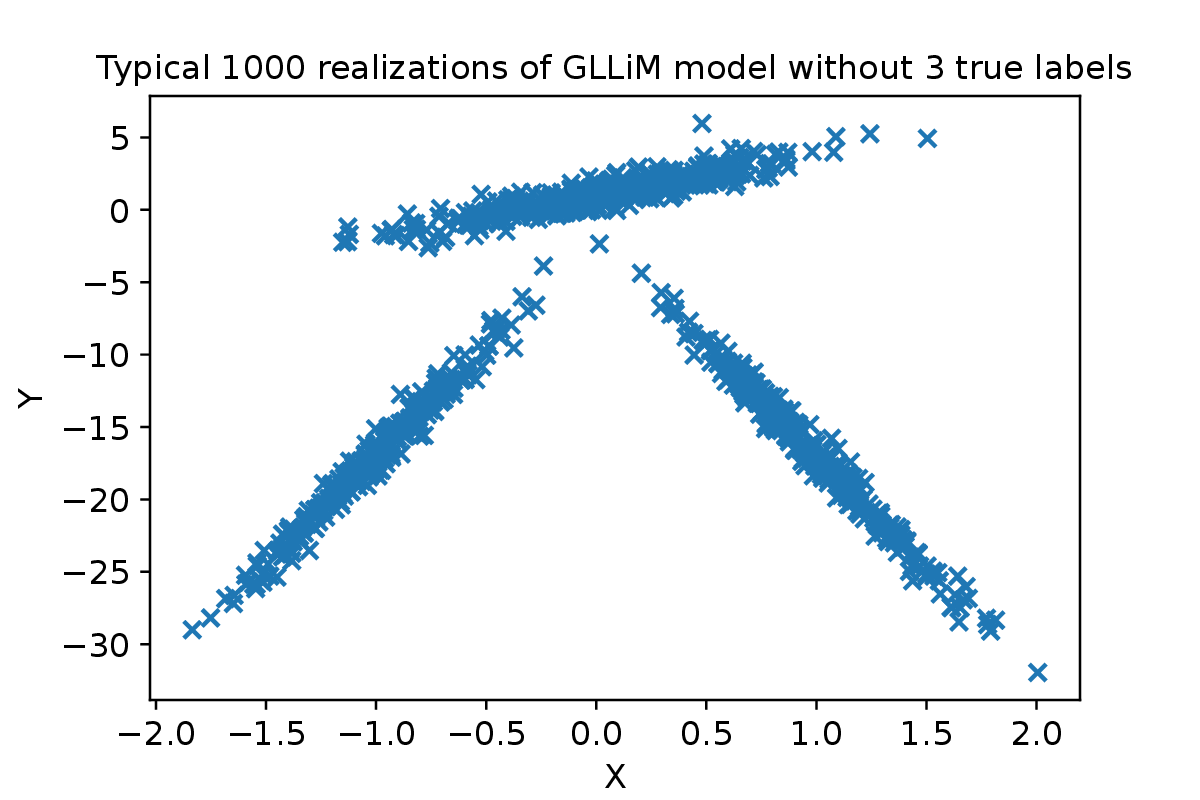
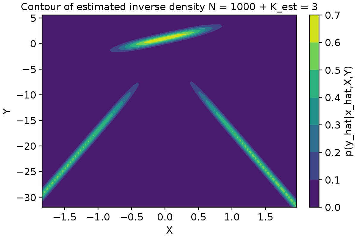
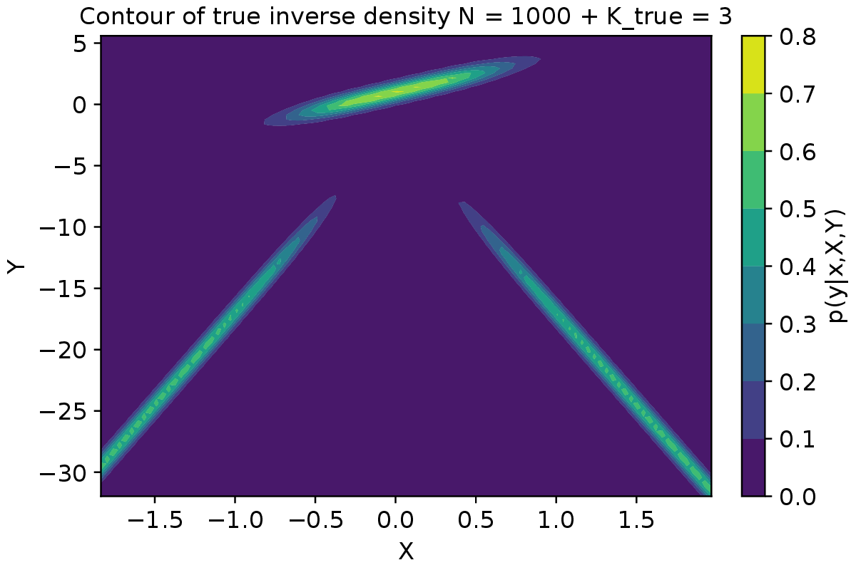
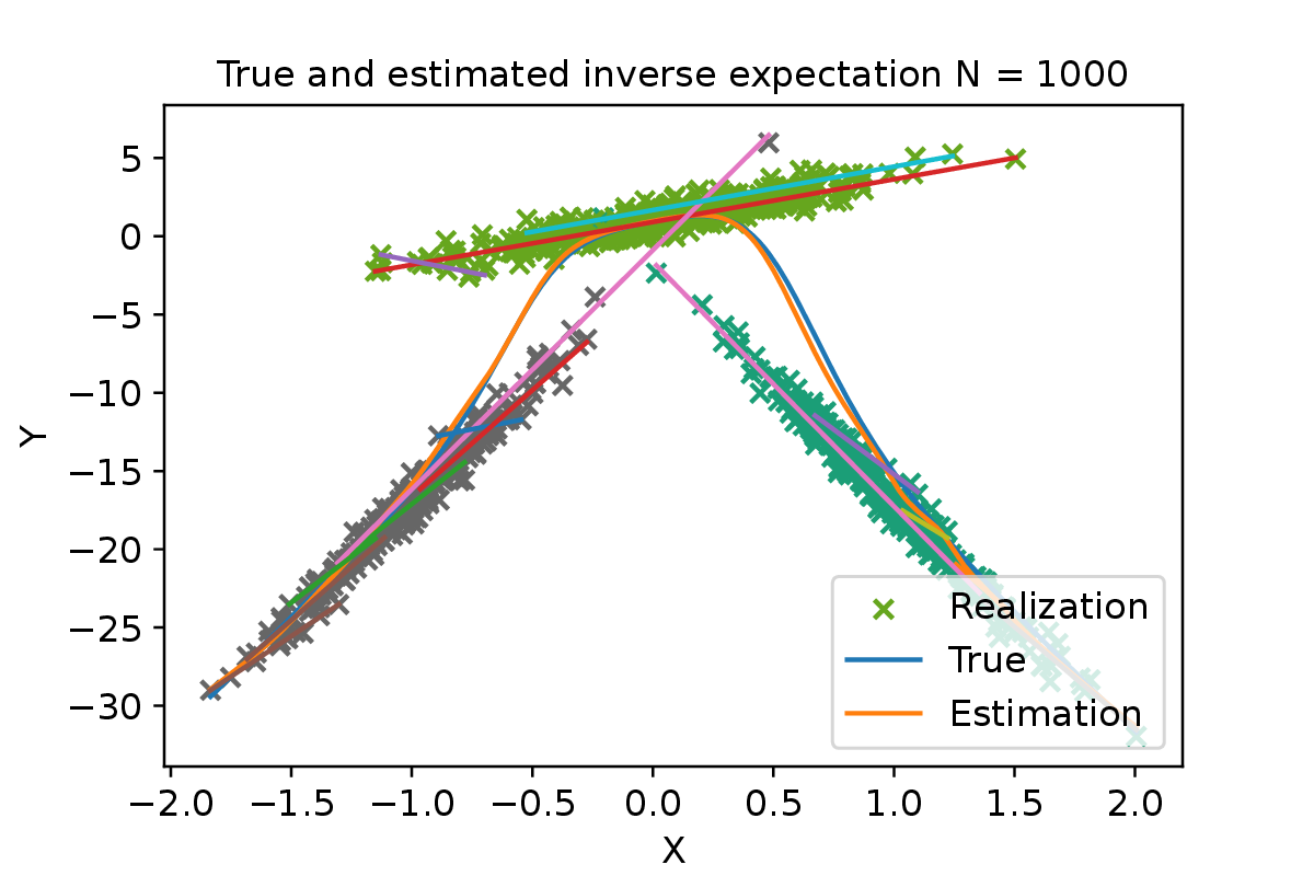
Figure 2a shows typical $N = 1, 000$ realisations of the true inverse cPDF from GLLiM, representing a $π$ -shape simulation with three clusters without labels.

6.2 Model selection, clustering and regression tasks via MTM-BNP-GLLiM

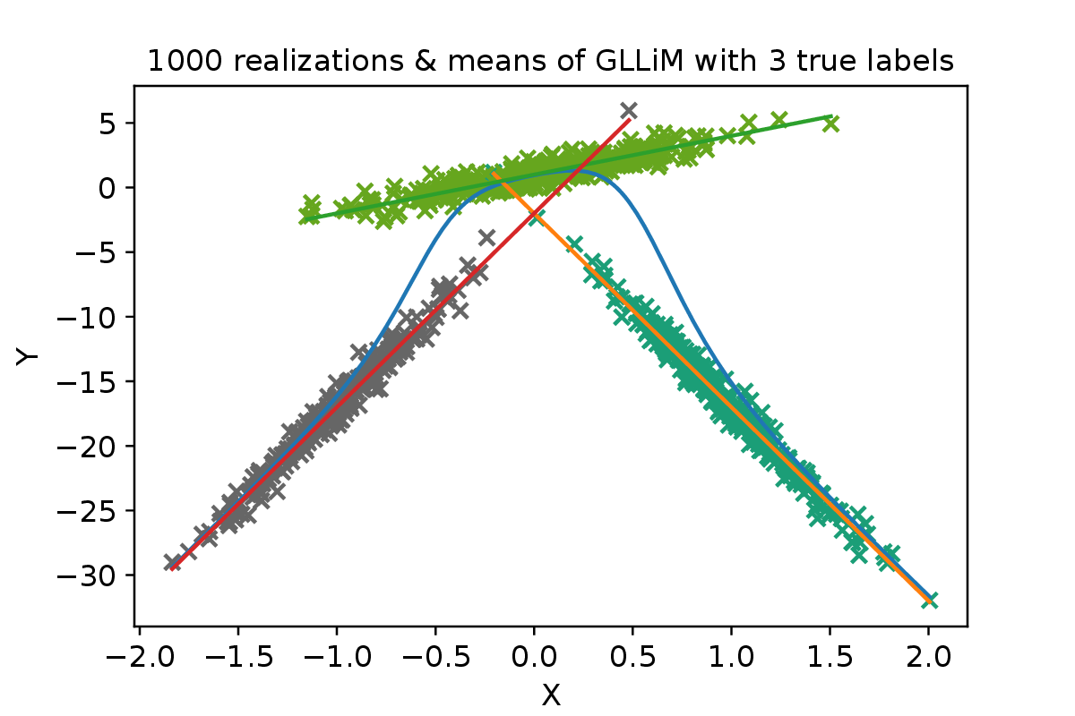
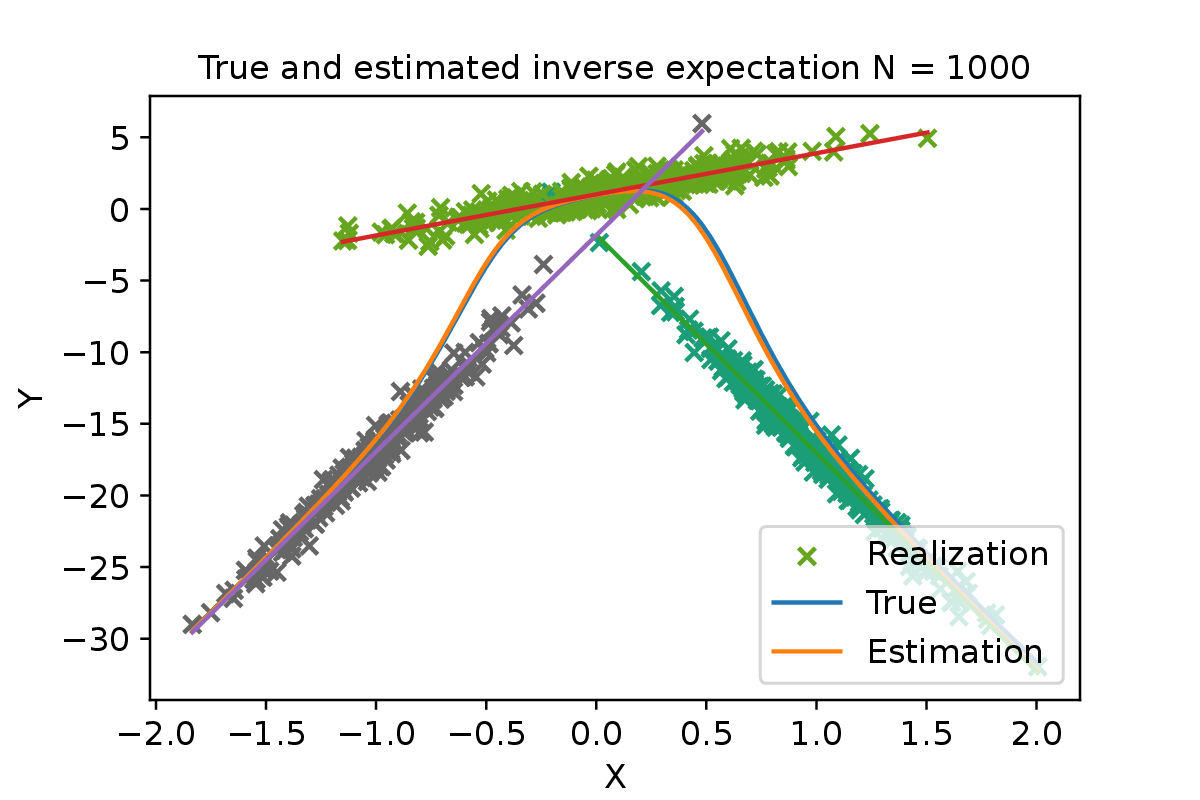
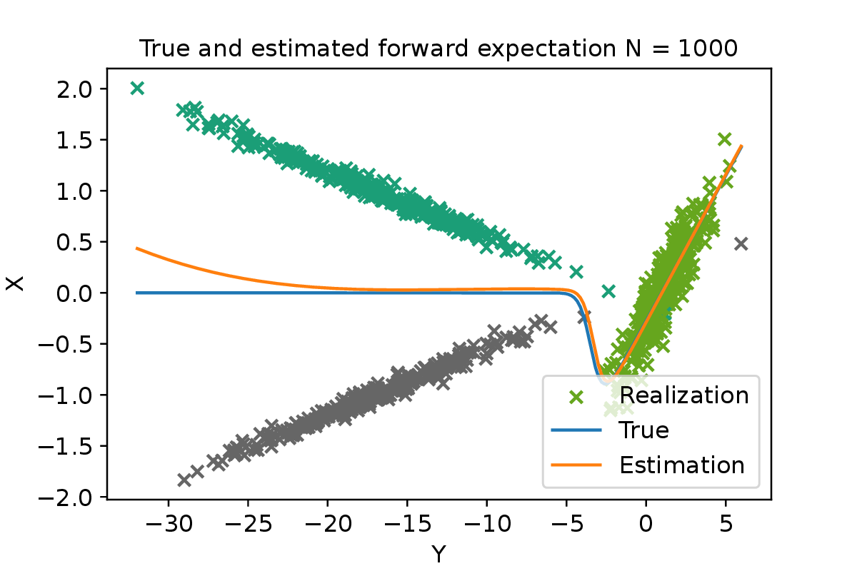
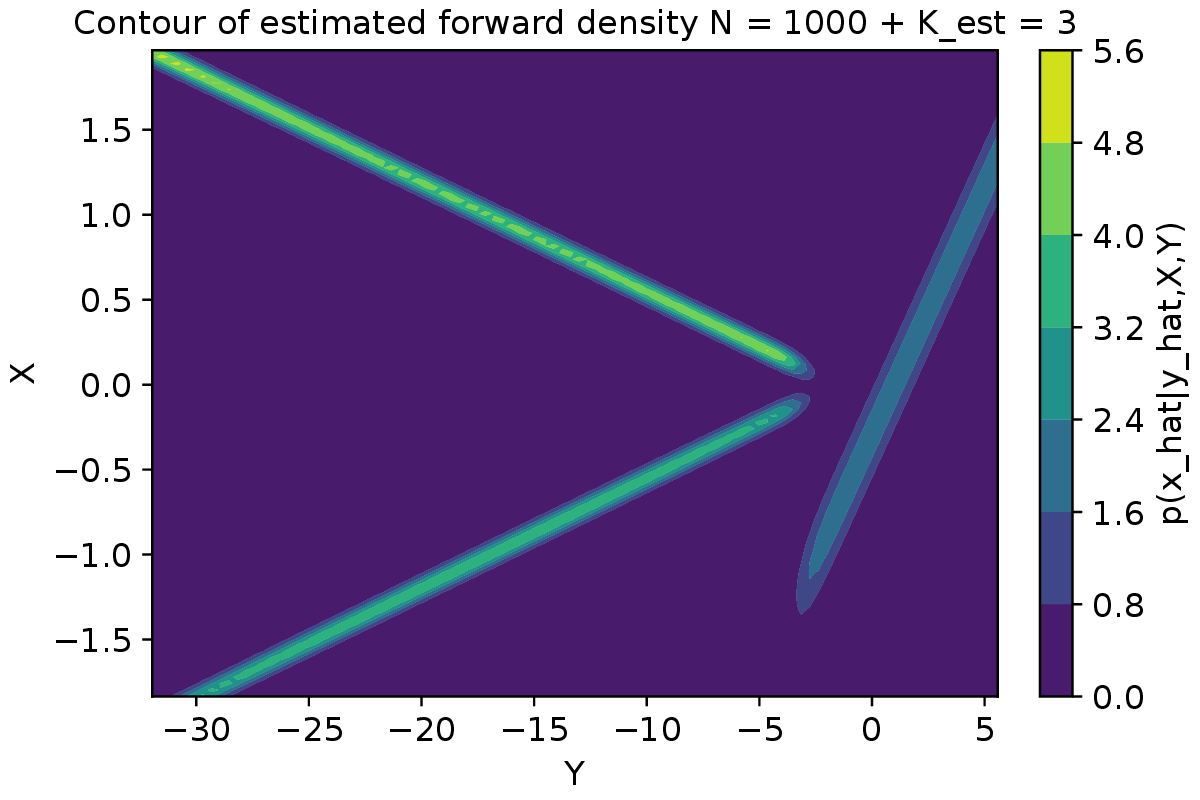
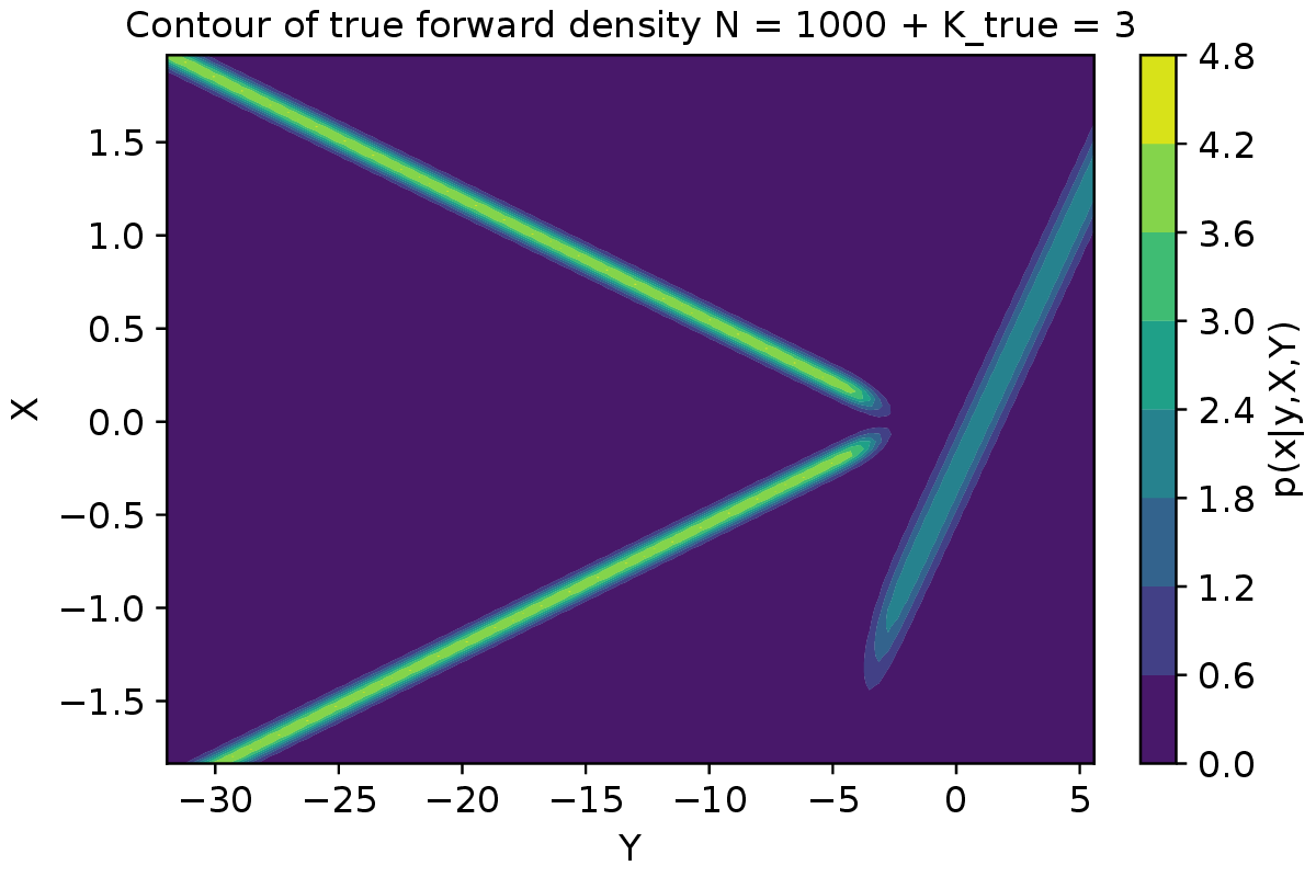
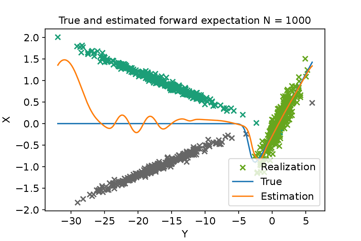
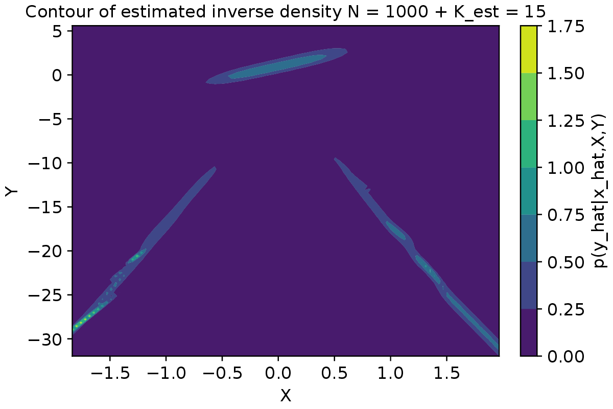
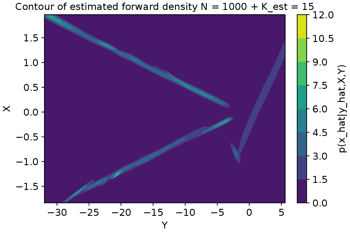
Our goal is to evaluate the inverse and forward cPDF, as well as the conditional means, to investigate the empirical performance of our MTM-BNP-GLLiM in the previous simulation. In Figure 2 it is clear that with the help of MTM Algorithm 1, MTM-BNP-GLLiM can simultaneously perform regression, clustering and model selection well. Without the MTM procedure, BNP-GLLiM performs poorly in model selection, clustering and cPDF estimation, except for conditional expectations as shown in Figure 3.

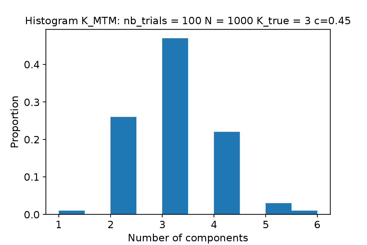
Refer to caption — (a) Typical realisations without labels.

Next, we illustrate the performance of the MTM algorithm when applied to the variational posterior from BNP-GLLiM. Specifically, the samples in our $100$ trials are drawn from $G_{V} = \sum_{k = 1}^{K} 𝔼_{q_{𝝉}} [π_{k} (𝝉)] δ_{𝜽_{k}}$ , wherere $𝔼_{q_{𝝉}} [π_{k} (𝝉)]$ and $𝜽_{k} = (𝝁_{k}, 𝐕_{k})$ are defined in (14) and (13), respectively. We know that for some constant $\tilde{C}$ , which depends on the covariance matrix $𝐕_{k}^{0}$ , the location parameters $𝝁^{0}_{k}$ and the weights $π_{k}^{0}$ , the contraction rate of mixing measures under the location Gaussian DP-MM is $\tilde{C} (\log (N))^{- 1 / 2}$ with respect to the $W_{2}$ -norm. Similar to Guha et al. (2021), our first attempt to choose $w_{N}$ to satisfy (17) is $w_{N} = (\frac{\log (\log (N))}{\log (N)})^{1 / 2}$ . In fact, we can choose any $w_{N}$ , as long as $\frac{w_{N}}{\log (N)^{- 1 / 2}} \to \infty$ , in order for $w_{N}$ to satisfy (17).

Since we only work with finite sample $N$ , it is not expected that the posterior probability for $K_{MTM} = K_{0}$ is close to $1$ and the input $c$ to Algorithm 1 should be chosen so that $\frac{\tilde{C}}{(\log (\log (N)))^{1 / 2}} \leq c$ . Furthermore, based on Equation (26) from Guha et al. (2021), with a useful lower bound on the posterior mass the mode, for any $1 > ϵ > 0$ , $(1 - ϵ) (1 - \sum_{k = 1}^{3} \frac{c_{0}^{r / 2}}{π_{k}^{0}}) > \frac{1}{2}$ , we hope to identify $K_{0}$ via the posterior mode with a reasonable estimate. To guarantee $K = K_{0}$ consistently using the posterior mode safety, we have to choose $c < c_{0}$ , with $c_{0}$ satisfying

(1 - ϵ) (1 - \sum_{k = 1}^{3} \frac{c_{0}^{r / 2}}{π_{k}^{0}}) > \frac{1}{2} \Leftrightarrow \frac{1 - 2 ϵ}{2 (1 - ϵ)} (\sum_{k = 1}^{3} \frac{1}{π_{k}^{0}})^{- 1} > c_{0}^{r / 2} > c^{r / 2} .

Therefore, we can choose

[\frac{1 - 2 ϵ}{4 (1 - ϵ)} (\sum_{k = 1}^{3} \frac{1}{π_{k}^{0}})^{- 1}]^{2 / r} = c_{0} > c, for all \frac{1}{2} > ϵ > 0 .

In particular, it is unrealistic to obtain the exact computation of the upper bound $c_{0}$ and the lower bound $\frac{\tilde{C}}{(\log (\log (N)))^{1 / 2}}$ . However, a reasonable estimate may be possible by considering a large range of $c$ , and show that there is a range where we can robustly identify the true number of components via the posterior mode. Guha et al. (2021) also used the same setting in their experiments. Figure 4 indicates that $c = 0.45$ leads to a quite good posterior mode in our experiments.

Although we do not have a theoretical result for the convergence rate of the variational posterior of BNP-GLLiM to the true data generating process, Figure 4 seems to suggest that MTM-BNP-GLLiM gives a comparable good result to the location Gaussian DP-MM in the simulation studies in Guha et al. (2021).

7 Perspectives

To address the dimensionality issue when $N$ is less than $D$ , we could incorporate sparsity penalty terms as described in the GLLiM context in Chamroukhi et al. (2019). Alternatively, we could impose additional structural restrictions, such as block-diagonal covariance matrices as in Blein-Nicolas et al. (2024)), which extends the GLLiM method to account for hidden module-structured regulatory networks of predictors through block-diagonal structures. In particular, Blein-Nicolas et al. (2024) applied their method to the prediction of drought-related traits $(L = 2)$ from protein abundance $(D = 973)$ in $N = 233$ maize genotypes. We leave for future research the intriguing but challenging questions of how to integrate BNP priors into the GLLiM model and how to establish posterior convergence theory in high-dimensional settings where $D ≫ N$ .

As indicated in Remark 2, there is a crucial need to formally establish general conditions on the prior, the likelihood and the variational class to characterise the convergence rate of the variational posterior of BNP-GLLiM to the true data generating process. Using the similar “prior mass and testing” conditions as in Ghosal et al. (2000), we believe that an interesting but challenging extension of the work on variational posterior unconditional distributions for MMs (Zhang and Gao, 2020) and on adaptive Bayesian estimation for MMs and MoE models but for true posterior distribution (Kruijer et al., 2010; Shen et al., 2013; Norets and Pati, 2017) can help shed some light and answer this important question. Furthermore, it is important to establish an extensional convergence property of our VBEM algorithm for BNP-GLLiM. This property is only known for GMM from Titterington and Wang (2006). A potential improvement of the VBEM algorithm developed for BNP-GLLiM can be achieved by combining it with MCMC, taking advantage of both inference approaches as in Ruiz and Titsias (2019). Finally, as mentioned in Section 6.2, the selection of a good data-driven tuning parameter $c$ as the same idea from the slope heuristic of Birgé and Massart (2007) is crucial for the success of the MTM procedure for any BNP model. We leave these interesting but challenging questions for future research.

Acknowledgments

We would like to express our sincere gratitude to the Reviewers and Editors for their valuable feedback, which has greatly enhanced the quality of this paper. All authors acknowledge funding from the Australian Research Council grant DP230100905, and from Inria Project WOMBAT.

References

H. Akaike (1974) A new look at the statistical model identification. IEEE Transactions on Automatic Control 19 (6), pp. 716–723. External Links: Document Cited by: §1. ↩ a
L. Alamichel, D. Bystrova, J. Arbel, and G. Kon Kam King (2024) Bayesian mixture models (in)consistency for the number of clusters. Scandinavian Journal of Statistics. Cited by: §1. ↩ a
J. Arbel, G. Kon Kam King, A. Lijoi, L. Nieto-Barajas, and I. Prünster (2021) BNPdensity: Bayesian nonparametric mixture modelling in R. Australian & New Zealand Journal of Statistics 63 (3), pp. 542–564. External Links: Link, Document Cited by: §1. ↩ a
S. Arlot (2019) Minimal penalties and the slope heuristics: a survey. Journal de la Société Française de Statistique 160 (3), pp. 1–106. Cited by: §1. ↩ a
F. Ascolani, A. Lijoi, G. Rebaudo, and G. Zanella (2022) Clustering consistency with Dirichlet process mixtures. Biometrika 110 (2), pp. 551–558. External Links: ISSN 1464-3510, Link, Document Cited by: §1. ↩ a
M. J. Beal and Z. Ghahramani (2003) The variational Bayesian EM algorithm for incomplete data: with application to scoring graphical model structures. Bayesian statistics 7 (453-464), pp. 210. Cited by: Appendix B. ↩ a
M. J. Beal (2003) Variational algorithms for approximate Bayesian inference. Ph.D. Thesis, University of London, University College London (United Kingdom). Cited by: Appendix B, Appendix B. ↩ a b
M. Berrettini, G. Galimberti, S. Ranciati, and T. B. Murphy (2024) Identifying Brexit voting patterns in the British house of commons: an analysis based on Bayesian mixture models with flexible concomitant covariate effects. Journal of the Royal Statistical Society Series C: Applied Statistics 73 (3), pp. 621–638. External Links: ISSN 0035-9254, Link, Document Cited by: §1. ↩ a
C. Biernacki, G. Celeux, and G. Govaert (2000) Assessing a mixture model for clustering with the integrated completed likelihood. IEEE Transactions on Pattern Analysis and Machine Intelligence 22 (7), pp. 719–725. External Links: Document Cited by: §1. ↩ a
L. Birgé and P. Massart (2007) Minimal penalties for Gaussian model selection. Probability Theory and Related Fields 138 (1), pp. 33–73. External Links: Link, Document Cited by: §1, §7. ↩ a b
C. M. Bishop (2006) Pattern Recognition and Machine Learning (Information Science and Statistics). Springer-Verlag, Berlin, Heidelberg. External Links: ISBN 0-387-31073-8 Cited by: Appendix B, §E.3, §E.5, §F.1.2, §F.4, §F.6. ↩ a b c d e f
D. M. Blei and M. I. Jordan (2006) Variational inference for Dirichlet process mixtures. Bayesian analysis 1 (1), pp. 121–143. Cited by: Appendix A, §E.3, §E.3, §F.4, §3. ↩ a b c d e
M. Blein-Nicolas, E. Devijver, M. Gallopin, and E. Perthame (2024) Nonlinear network-based quantitative trait prediction from biological data. Journal of the Royal Statistical Society Series C: Applied Statistics, pp. qlae012. Cited by: §1, §7, Remark 1. ↩ a b c d
F. Boux, F. Forbes, J. Arbel, B. Lemasson, and E. L. Barbier (2021) Bayesian inverse regression for vascular magnetic resonance fingerprinting. IEEE Transactions on Medical Imaging 40 (7), pp. 1827–1837. Cited by: §1. ↩ a
G. Celeux, S. Frühwirth-Schnatter, and C. P. Robert (2019) Model selection for mixture models–perspectives and strategies. In Handbook of mixture analysis, pp. 117–154. Cited by: §1. ↩ a
L. Chaari, T. Vincent, F. Forbes, M. Dojat, and P. Ciuciu (2013) Fast joint detection-estimation of evoked brain activity in event-related fMRI using a variational approach. IEEE transactions on Medical Imaging 32 (5), pp. 821–837. Cited by: Appendix B. ↩ a
F. Chamroukhi, F. Lecocq, and H. D. Nguyen (2019) Regularized Estimation and Feature Selection in Mixtures of Gaussian-Gated Experts Models. In Statistics and Data Science, H. Nguyen (Ed.), Singapore, pp. 42–56. External Links: ISBN 978-981-15-1960-4 Cited by: §7. ↩ a
F. Chamroukhi, A. Samé, G. Govaert, and P. Aknin (2010) A hidden process regression model for functional data description. Application to curve discrimination. Neurocomputing 73 (7-9), pp. 1210–1221. Cited by: §6.1. ↩ a
Z. Chen, Y. Deng, Y. Wu, Q. Gu, and Y. Li (2022) Towards Understanding the Mixture-of-Experts Layer in Deep Learning. In Advances in Neural Information Processing Systems, A. H. Oh, A. Agarwal, D. Belgrave, and K. Cho (Eds.), External Links: Link Cited by: §1. ↩ a
P. De Blasi, S. Favaro, A. Lijoi, R. H. Mena, I. Prünster, and M. Ruggiero (2015) Are Gibbs-type priors the most natural generalization of the Dirichlet process?. IEEE transactions on pattern analysis and machine intelligence 37 (2), pp. 212–229. Cited by: Appendix A. ↩ a
A. Deleforge, F. Forbes, and R. Horaud (2015) High-dimensional regression with gaussian mixtures and partially-latent response variables. Statistics and Computing 25 (5), pp. 893–911. External Links: ISSN 1573-1375, Link, Document Cited by: §E.1, §1, §2.1, §2.2, §2.2, Remark 1. ↩ a b c d e f g h i
J. Delon and A. Desolneux (2020) A Wasserstein-type distance in the space of Gaussian mixture models. SIAM Journal on Imaging Sciences 13 (2), pp. 936–970. Cited by: Definition 5.1. ↩ a
A. P. Dempster, N. M. Laird, and D. B. Rubin (1977) Maximum Likelihood from Incomplete Data Via the EM Algorithm. Journal of the Royal Statistical Society: Series B (Methodological) 39 (1), pp. 1–22. External Links: ISSN 0035-9246, Link, Document Cited by: Appendix B. ↩ a
T. G. Do, H. K. Le, T. Nguyen, Q. Pham, B. T. Nguyen, T. Doan, C. Liu, S. Ramasamy, X. Li, and S. HOI (2023) HyperRouter: Towards Efficient Training and Inference of Sparse Mixture of Experts. In Proceedings of the 2023 Conference on Empirical Methods in Natural Language Processing, Singapore. Cited by: §1. ↩ a
J.-B. Durand, F. Forbes, C.D. Phan, L. Truong, H.D. Nguyen, and F. Dama (2022) Bayesian non-parametric spatial prior for traffic crash risk mapping: A case study of Victoria, Australia. Australian & New Zealand Journal of Statistics 64 (2), pp. 171–204. External Links: Link, Document Cited by: Appendix A, §1, §3.3. ↩ a b c
M. D. Escobar and M. West (1995) Bayesian Density Estimation and Inference Using Mixtures. Journal of the American Statistical Association 90 (430), pp. 577–588. External Links: Link, Document Cited by: §1. ↩ a
S. Favaro, A. Lijoi, C. Nava, B. Nipoti, I. Pruenster, and Y. W. Teh (2016) On the stick-breaking representation for homogeneous NRMIs. Bayesian Analysis 11 (3), pp. 697–724. Cited by: Appendix A. ↩ a
T. S. Ferguson (1973) A Bayesian Analysis of Some Nonparametric Problems. The Annals of Statistics 1 (2), pp. 209 – 230. External Links: Link, Document Cited by: Appendix A. ↩ a
F. Forbes, A. Arnaud, B. Lemasson, and E. Barbier (2019) Component elimination strategies to fit mixtures of multiple scale distributions. In RSSDS 2019 - Research School on Statistics and Data Science, Communications in Computer and Information Science, Vol. 1150, Melbourne, Australia, pp. 81–95. External Links: Link, Document Cited by: §1. ↩ a
F. Forbes, H. D. Nguyen, T. Nguyen, and J. Arbel (2022a) Mixture of expert posterior surrogates for approximate Bayesian computation. In JDS 2022 - 53èmes Journées de Statistique de la Société Française de Statistique (SFdS), Lyon, France. Cited by: §1. ↩ a
F. Forbes, H. D. Nguyen, T. Nguyen, and J. Arbel (2022b) Summary statistics and discrepancy measures for approximate Bayesian computation via surrogate posteriors. Statistics and Computing 32 (5), pp. 85. External Links: ISSN 1573-1375, Link, Document Cited by: §1. ↩ a
R. Foygel and M. Drton (2010) Extended Bayesian Information Criteria for Gaussian Graphical Models. In Advances in Neural Information Processing Systems, J. Lafferty, C. Williams, J. Shawe-Taylor, R. Zemel, and A. Culotta (Eds.), Vol. 23. External Links: Link Cited by: §1. ↩ a
S. Frühwirth-Schnatter, D. Hosszejni, and H. F. Lopes (2024) Sparse Bayesian Factor Analysis When the Number of Factors Is Unknown. Bayesian Analysis, pp. 1 – 48. Note: Publisher: International Society for Bayesian Analysis External Links: Link, Document Cited by: §1. ↩ a
S. Frühwirth-Schnatter, C. Pamminger, A. Weber, and R. Winter-Ebmer (2012) Labor market entry and earnings dynamics: Bayesian inference using mixtures-of-experts Markov chain clustering. Journal of Applied Econometrics 27 (7), pp. 1116–1137. External Links: Link, Document Cited by: §1. ↩ a
S. Frühwirth-Schnatter, S. Pittner, A. Weber, and R. Winter-Ebmer (2018) Analysing plant closure effects using time-varying mixture-of-experts Markov chain clustering. The Annals of Applied Statistics 12 (3), pp. 1796 – 1830. Note: Publisher: Institute of Mathematical Statistics External Links: Link, Document Cited by: §1. ↩ a
S. Frühwirth-Schnatter (2019) Keeping the balance—Bridge sampling for marginal likelihood estimation in finite mixture, mixture of experts and Markov mixture models. Brazilian Journal of Probability and Statistics 33 (4), pp. 706 – 733. External Links: Link, Document Cited by: §1. ↩ a
F. Gao and A. v. d. Vaart (2016) Posterior contraction rates for deconvolution of Dirichlet-Laplace mixtures. Electronic Journal of Statistics 10 (1), pp. 608 – 627. External Links: Link, Document Cited by: §5.1. ↩ a
C. R. Genovese and L. Wasserman (2000) Rates of convergence for the Gaussian mixture sieve. The Annals of Statistics 28 (4), pp. 1105 – 1127. External Links: Link, Document Cited by: §1. ↩ a
S. Ghosal, J. K. Ghosh, and A. W. v. d. Vaart (2000) Convergence rates of posterior distributions. The Annals of Statistics 28 (2), pp. 500 – 531. External Links: Link, Document Cited by: §7. ↩ a
S. Ghosal and A. Van der Vaart (2017) Fundamentals of nonparametric Bayesian inference. Vol. 44, Cambridge University Press. External Links: ISBN 0-521-87826-8 Cited by: Appendix A, §E.3, §1. ↩ a b c
I. C. Gormley and S. Frühwirth-Schnatter (2019) Mixture of experts models. In Handbook of mixture analysis, pp. 271–307. Cited by: §1. ↩ a
P. J. Green and S. Richardson (2001) Modelling Heterogeneity With and Without the Dirichlet Process. Scandinavian Journal of Statistics 28 (2), pp. 355–375. External Links: Link, Document Cited by: §1. ↩ a
A. Guha, N. Ho, and X. Nguyen (2021) On posterior contraction of parameters and interpretability in Bayesian mixture modeling. Bernoulli 27 (4), pp. 2159 – 2188. External Links: Link, Document Cited by: §1, §1, item i, §5.1, §5.2, §5.2, §6.2, §6.2, §6.2. ↩ a b c d e f g h i j k
N. L. Hjort, C. Holmes, P. Müller, and S. G. Walker (Eds.) (2010) Bayesian Nonparametrics. Cambridge Series in Statistical and Probabilistic Mathematics, Cambridge University Press. External Links: ISBN 978-0-521-51346-3, Link, Document Cited by: §1. ↩ a
N. Ho and X. Nguyen (2016a) Convergence rates of parameter estimation for some weakly identifiable finite mixtures. The Annals of Statistics 44 (6), pp. 2726 – 2755. External Links: Link, Document Cited by: §1. ↩ a
N. Ho and X. Nguyen (2016b) On strong identifiability and convergence rates of parameter estimation in finite mixtures. Electronic Journal of Statistics 10 (1), pp. 271–307. Cited by: §1, §5.1, §5.1. ↩ a b c
N. Ho, C. Yang, and M. I. Jordan (2022) Convergence Rates for Gaussian Mixtures of Experts. Journal of Machine Learning Research 23 (323), pp. 1–81. External Links: Link Cited by: §1. ↩ a
B. Hoadley (1970) A Bayesian Look at Inverse Linear Regression. Journal of the American Statistical Association 65 (329), pp. 356–369. External Links: Link, Document Cited by: §1. ↩ a
S. Ingrassia, S. C. Minotti, and G. Vittadini (2012) Local Statistical Modeling via a Cluster-Weighted Approach with Elliptical Distributions. Journal of Classification 29 (3), pp. 363–401. External Links: ISSN 1432-1343, Link, Document Cited by: §2.2. ↩ a
H. Ishwaran and L. F. James (2001) Gibbs Sampling Methods for Stick-Breaking Priors. Journal of the American Statistical Association 96 (453), pp. 161–173. External Links: ISSN 0162-1459, Link, Document Cited by: Appendix A. ↩ a
R. A. Jacobs, M. I. Jordan, S. J. Nowlan, and G. E. Hinton (1991) Adaptive mixtures of local experts. Neural computation 3 (1), pp. 79–87. Cited by: §1. ↩ a
W. Jiang and M. A. Tanner (1999) Hierarchical mixtures-of-experts for exponential family regression models: approximation and maximum likelihood estimation. Annals of Statistics, pp. 987–1011. Cited by: §1. ↩ a
L. Kock, N. Klein, and D. J. Nott (2022) Variational inference and sparsity in high-dimensional deep Gaussian mixture models. Statistics and Computing 32 (5), pp. 70. External Links: ISSN 1573-1375, Link, Document Cited by: §1. ↩ a
W. Kruijer, J. Rousseau, and A. v. d. Vaart (2010) Adaptive Bayesian density estimation with location-scale mixtures. Electronic Journal of Statistics 4 (none), pp. 1225 – 1257. External Links: Link, Document Cited by: §7. ↩ a
B. Kugler, F. Forbes, and S. Douté (2022) Fast Bayesian Inversion for high dimensional inverse problems. Statistics and Computing 32 (2). Cited by: §1. ↩ a
S. Lathuilière, R. Juge, P. Mesejo, R. Muñoz-Salinas, and R. Horaud (2017) Deep mixture of linear inverse regressions applied to head-pose estimation. In Proceedings of the IEEE Conference on Computer Vision and Pattern Recognition, pp. 4817–4825. Cited by: §1. ↩ a
K. Li (1991) Sliced Inverse Regression for Dimension Reduction. Journal of the American Statistical Association 86 (414), pp. 316–327. External Links: ISSN 01621459, Link, Document Cited by: §1, §2.1. ↩ a b
N. Li, W. Li, Y. Jiang, and S. Xia (2022) Deep Dirichlet process mixture models. In Proceedings of the Thirty-Eighth Conference on Uncertainty in Artificial Intelligence, J. Cussens and K. Zhang (Eds.), Proceedings of Machine Learning Research, Vol. 180, pp. 1138–1147. External Links: Link Cited by: §1. ↩ a
H. Lü, J. Arbel, and F. Forbes (2020) Bayesian nonparametric priors for hidden Markov random fields. Statistics and Computing 30 (4), pp. 1015–1035. External Links: ISSN 1573-1375, Link, Document Cited by: Appendix A, Appendix A, §3.2. ↩ a b c
C. Luo and S. Sun (2017) Variational Mixtures of Gaussian Processes for Classification. In Proceedings of the Twenty-Sixth International Joint Conference on Artificial Intelligence, IJCAI-17, pp. 4603–4609. External Links: Link, Document Cited by: §3.3. ↩ a
S. N. Maceachern and P. Müller (1998) Estimating Mixture of Dirichlet Process Models. Journal of Computational and Graphical Statistics 7 (2), pp. 223–238. External Links: Link, Document Cited by: §1, §1. ↩ a b
G. J. McLachlan and D. Peel (2000) Finite Mixture Models. John Wiley & Sons. Cited by: §1. ↩ a
G. J. McLachlan and T. Krishnan (1997) The EM algorithm and extensions. Wiley, New York, USA. Cited by: Appendix B. ↩ a
J. W. Miller and M. T. Harrison (2014) Inconsistency of Pitman-Yor Process Mixtures for the Number of Components. Journal of Machine Learning Research 15 (96), pp. 3333–3370. External Links: Link Cited by: §1. ↩ a
L. Montuelle and E. Le Pennec (2014) Mixture of Gaussian regressions model with logistic weights, a penalized maximum likelihood approach. Electronic Journal of Statistics 8 (1), pp. 1661–1695. Cited by: §6.1. ↩ a
R. M. Neal and G. E. Hinton (1998) A View of the EM Algorithm that Justifies Incremental, Sparse, and other Variants. In Learning in Graphical Models, M. I. Jordan (Ed.), pp. 355–368. External Links: ISBN 978-94-011-5014-9, Link, Document Cited by: Appendix B. ↩ a
R. M. Neal (2000) Markov Chain Sampling Methods for Dirichlet Process Mixture Models. Journal of Computational and Graphical Statistics 9 (2), pp. 249–265. External Links: Link, Document Cited by: §1. ↩ a
D. T. Nguyen, S. Jacquemoud, A. Lucas, S. Douté, C. Ferrari, S. Coustance, S. Marcq, and A. Meygret (2024a) Unveiling the Characteristics of the Lunar Surface by Massive Inversion of a Photometric Model. In LPI Contributions, LPI Contributions, Vol. 3040, pp. 1998. Cited by: §1. ↩ a
D. N. Nguyen and Z. Li (2024) Joint learning of Gaussian graphical models in heterogeneous dependencies of high-dimensional transcriptomic data. In The 16th Asian Conference on Machine Learning (Conference Track), External Links: Link Cited by: §1. ↩ a
H. D. Nguyen, F. Chamroukhi, and F. Forbes (2019) Approximation results regarding the multiple-output Gaussian gated mixture of linear experts model. Neurocomputing 366, pp. 208–214. External Links: ISSN 0925-2312, Link, Document Cited by: §1. ↩ a
H. D. Nguyen and F. Chamroukhi (2018) Practical and theoretical aspects of mixture-of-experts modeling: An overview. Wiley Interdisciplinary Reviews: Data Mining and Knowledge Discovery 8 (4), pp. e1246. Cited by: §1. ↩ a
H. D. Nguyen, L. R. Lloyd-Jones, and G. J. McLachlan (2016) A universal approximation theorem for mixture-of-experts models. Neural computation 28 (12), pp. 2585–2593. Cited by: §1. ↩ a
H. D. Nguyen, D. Fryer, and G. J. McLachlan (2022a) Order selection with confidence for finite mixture models. Journal of the Korean Statistical Society. External Links: ISSN 2005-2863, Link, Document Cited by: §1. ↩ a
H. D. Nguyen, T. Nguyen, F. Chamroukhi, and G. J. McLachlan (2021a) Approximations of conditional probability density functions in Lebesgue spaces via mixture of experts models. Journal of Statistical Distributions and Applications 8 (1), pp. 13. External Links: ISSN 2195-5832, Link, Document Cited by: §1. ↩ a
H. Nguyen, P. Akbarian, T. Nguyen, and N. Ho (2024b) A General Theory for Softmax Gating Multinomial Logistic Mixture of Experts. In Proceedings of The 41st International Conference on Machine Learning, Cited by: §1. ↩ a
H. Nguyen, T. Nguyen, and N. Ho (2023a) Demystifying Softmax Gating in Gaussian Mixture of Experts. In Advances in Neural Information Processing Systems, Cited by: §1. ↩ a
H. Nguyen, T. Nguyen, K. Nguyen, and N. Ho (2024c) Towards Convergence Rates for Parameter Estimation in Gaussian-gated Mixture of Experts. In Proceedings of The 27th International Conference on Artificial Intelligence and Statistics, S. Dasgupta, S. Mandt, and Y. Li (Eds.), Proceedings of Machine Learning Research, Vol. 238, pp. 2683–2691. External Links: Link Cited by: §1. ↩ a
T. Nguyen and E. Bonilla (2014) Fast Allocation of Gaussian Process Experts. In Proceedings of the 31st International Conference on Machine Learning, E. P. Xing and T. Jebara (Eds.), Proceedings of Machine Learning Research, Vol. 32, Bejing, China, pp. 145–153. External Links: Link Cited by: §3.3. ↩ a
T. Nguyen, F. Chamroukhi, H. D. Nguyen, and G. J. McLachlan (2023b) Approximation of probability density functions via location-scale finite mixtures in Lebesgue spaces. Communications in Statistics - Theory and Methods 52 (14), pp. 5048–5059. External Links: Link, Document Cited by: §1. ↩ a
T. Nguyen, F. Chamroukhi, H. D. Nguyen, and F. Forbes (2021b) Non-asymptotic model selection in block-diagonal mixture of polynomial experts models. Preprint. arXiv:2104.08959. External Links: Link Cited by: §1. ↩ a
T. Nguyen, F. Chamroukhi, H. D. Nguyen, and F. Forbes (2022b) Model selection by penalization in mixture of experts models with a non-asymptotic approach. In JDS 2022 - 53èmes Journées de Statistique de la Société Française de Statistique (SFdS), Lyon, France. Cited by: §1. ↩ a
T. Nguyen, D. N. Nguyen, H. D. Nguyen, and F. Chamroukhi (2023c) A non-asymptotic theory for model selection in high-dimensional mixture of experts via joint rank and variable selection. In AJCAI Australasian Joint Conference on Artificial Intelligence 2023, External Links: Link Cited by: §1. ↩ a
T. Nguyen, H. D. Nguyen, F. Chamroukhi, and G. J. McLachlan (2023d) Non-asymptotic oracle inequalities for the Lasso in high-dimensional mixture of experts. arXiv:2009.10622. External Links: Link Cited by: §1. ↩ a
T. Nguyen, H. D. Nguyen, F. Chamroukhi, and F. Forbes (2022c) A non-asymptotic approach for model selection via penalization in high-dimensional mixture of experts models. Electronic Journal of Statistics 16 (2), pp. 4742 – 4822. External Links: Link, Document Cited by: §1, §2.2, §6.1. ↩ a b c
T. Nguyen, H. D. Nguyen, F. Chamroukhi, and G. J. McLachlan (2020) Approximation by finite mixtures of continuous density functions that vanish at infinity. Cogent Mathematics & Statistics 7 (1), pp. 1750861. External Links: ISSN null, Link, Document Cited by: §1. ↩ a
T. Nguyen (2021) Model Selection and Approximation in High-dimensional Mixtures of Experts Models: from Theory to Practice. PhD Thesis, Normandie Université, (en). External Links: Link Cited by: §1. ↩ a
X. Nguyen (2013) Convergence of latent mixing measures in finite and infinite mixture models. The Annals of Statistics 41 (1), pp. 370–400. External Links: Link, Document Cited by: §1, §5.1, §5.1. ↩ a b c
A. Norets and D. Pati (2017) Adaptive Bayesian estimation of conditional densities. Econometric Theory 33 (4), pp. 980–1012. External Links: Document Cited by: §7. ↩ a
A. Norets (2010) Approximation of conditional densities by smooth mixtures of regressions. The Annals of Statistics 38 (3), pp. 1733 – 1766. External Links: Link, Document Cited by: §1. ↩ a
E. Perthame, F. Forbes, and A. Deleforge (2018) Inverse regression approach to robust nonlinear high-to-low dimensional mapping. Journal of Multivariate Analysis 163 (C), pp. 1–14. Cited by: §2.2. ↩ a
J. Pitman and M. Yor (1997) The two-parameter Poisson-Dirichlet distribution derived from a stable subordinator. The Annals of Probability 25 (2), pp. 855–900. External Links: Document Cited by: Appendix A, Appendix A, §3. ↩ a b c
A. Rakhlin, D. Panchenko, and S. Mukherjee (2005) Risk bounds for mixture density estimation. ESAIM: PS 9, pp. 220–229. External Links: Link, Document Cited by: §1. ↩ a
J. Rousseau and K. Mengersen (2011) Asymptotic behaviour of the posterior distribution in overfitted mixture models. Journal of the Royal Statistical Society: Series B (Statistical Methodology) 73 (5), pp. 689–710. External Links: Link, Document Cited by: §1. ↩ a
F. Ruiz and M. Titsias (2019) A Contrastive Divergence for Combining Variational Inference and MCMC. In Proceedings of the 36th International Conference on Machine Learning, K. Chaudhuri and R. Salakhutdinov (Eds.), Proceedings of Machine Learning Research, Vol. 97, pp. 5537–5545. External Links: Link Cited by: §7. ↩ a
G. Schwarz (1978) Estimating the dimension of a model. The Annals of Statistics 6 (2), pp. 461–464. Cited by: §1. ↩ a
J. Sethuraman (1994) A constructive definition of Dirichlet priors. Statistica Sinica 4, pp. 639–650. Cited by: Appendix A. ↩ a
W. Shen, S. T. Tokdar, and S. Ghosal (2013) Adaptive Bayesian multivariate density estimation with Dirichlet mixtures. Biometrika 100 (3), pp. 623–640. Cited by: §1, §7. ↩ a b
C. Sin and H. White (1996) Information criteria for selecting possibly misspecified parametric models. Journal of Econometrics 71 (1), pp. 207–225. External Links: ISSN 0304-4076, Link, Document Cited by: §1. ↩ a
M. Svensén and C. M. Bishop (2005) Robust Bayesian mixture modelling. Neurocomputing 64, pp. 235–252. External Links: ISSN 0925-2312, Link, Document Cited by: §3.3. ↩ a
D. M. Titterington and B. Wang (2006) Convergence properties of a general algorithm for calculating variational Bayesian estimates for a normal mixture model. Bayesian Analysis 1 (3), pp. 625 – 650. External Links: Link, Document Cited by: §7. ↩ a
C. Villani (2003) Topics in optimal transportation. Graduate Studies in Mathematics, Vol. 58, American Mathematical Society. External Links: ISBN 0-8218-3312-X Cited by: §5.1. ↩ a
C. Villani (2009) Optimal transport: old and new. Vol. 338, Springer. Cited by: §5.1. ↩ a
C. Wang, J. Paisley, and D. M. Blei (2011) Online Variational Inference for the Hierarchical Dirichlet Process. In Proceedings of the Fourteenth International Conference on Artificial Intelligence and Statistics, G. Gordon, D. Dunson, and M. Dudík (Eds.), Proceedings of Machine Learning Research, Vol. 15, Fort Lauderdale, FL, USA, pp. 752–760. External Links: Link Cited by: §3. ↩ a
J. Westerhout, T. Nguyen, X. Guo, and H. D. Nguyen (2024) On the Asymptotic Distribution of the Minimum Empirical Risk. In Forty-first International Conference on Machine Learning, External Links: Link Cited by: §1. ↩ a
D. Wu and J. Ma (2018) A Two-Layer Mixture Model of Gaussian Process Functional Regressions and Its MCMC EM Algorithm. IEEE Transactions on Neural Networks and Learning Systems 29 (10), pp. 4894–4904. External Links: Document Cited by: §3.3. ↩ a
L. Xu, M. Jordan, and G. E. Hinton (1995) An Alternative Model for Mixtures of Experts. In Advances in Neural Information Processing Systems, G. Tesauro, D. Touretzky, and T. Leen (Eds.), Vol. 7. External Links: Link Cited by: §1. ↩ a
C. Yuan and C. Neubauer (2008) Variational Mixture of Gaussian Process Experts. In Advances in Neural Information Processing Systems, D. Koller, D. Schuurmans, Y. Bengio, and L. Bottou (Eds.), Vol. 21. External Links: Link Cited by: §3.3. ↩ a
S. E. Yuksel, J. N. Wilson, and P. D. Gader (2012) Twenty Years of Mixture of Experts. IEEE Transactions on Neural Networks and Learning Systems 23 (8), pp. 1177–1193. External Links: ISSN 2162-2388 VO - 23, Document Cited by: §1. ↩ a
G. Zens (2019) Bayesian shrinkage in mixture-of-experts models: identifying robust determinants of class membership. Advances in Data Analysis and Classification 13 (4), pp. 1019–1051. External Links: ISSN 1862-5355, Link, Document Cited by: §1. ↩ a
F. Zhang and C. Gao (2020) Convergence rates of variational posterior distributions. The Annals of Statistics 48 (4), pp. 2180 – 2207. External Links: Link, Document Cited by: §7. ↩ a

Supplementary Materials for
“Bayesian nonparametric mixture of experts for inverse problems”

In this supplementary material, we first recall the standard Bayesian nonparametric priors and variational Bayesian expectation-maximisation principle in Appendices A and B, respectively. Then, all specifications of the VBEM for the BNP-GLLiM model, the evidence lower bound and the technical proofs that are not included in the main paper are placed in Appendices C, D and E. . Finally, Appendix F proposes a more general model with a hyper prior on the gating parameters, referred to as BNP-GLLiM2.

Appendix A Bayesian nonparametric priors

Stick-breaking construction of Dirichlet process.

Note that the Dirichlet process (DP) (Ferguson, 1973) is a central BNP prior and is the infinite-dimensional generalization of the Dirichlet distribution. Therefore, for the sake of completeness, let us first recall the definition of the DP. A DP on the space $𝒢$ is defined as a random process characterized by a concentration parameter $α$ and a base distribution $G_{0}$ , denoted by $G \sim DP (α, G_{0})$ , such that for any finite partition ${A_{1}, \dots, A_{p}}$ of $𝒢$ , the random vector $(G (A_{1}), \dots, G (A_{p}))$ is Dirichlet distributed:

(G (A_{1}), \dots, G (A_{p})) \sim Dir (α G_{0} (A_{1}), \dots, α G_{0} (A_{p})) .

We use the stick-breaking construction of the DP $G$ (SBDP), due to Sethuraman (1994):

	$𝜽^{0}_{k} ∣ G_{0} \overset{iid}{\sim} G_{0}, k \in ℕ^{⋆},$
	$τ_{k} ∣ α \overset{iid}{\sim} Beta (τ_{k} ∣ 1, α), k \in ℕ^{⋆},$
	$π_{k} (𝝉) = τ_{k} \prod_{l = 1}^{k - 1} (1 - τ_{l}), k \in ℕ^{⋆},$
	$G = \sum_{k = 1}^{\infty} π_{k} (𝝉) δ_{𝜽^{0}_{k}} \sim DP (α, G_{0}) .$

Pitman–Yor process.

As a generalized version of the Dirichlet process, in the Pitman–Yor process (PYP) (Pitman and Yor, 1997), the $τ_{k}$ ’s are independent ( $\overset{ind}{\sim}$ ) but not identically distributed. Specifically,

	$𝜽^{0}_{k} ∣ G_{0} \overset{iid}{\sim} G_{0}, k \in ℕ^{⋆},$
	$τ_{k} ∣ α, σ \overset{ind}{\sim} Beta (1 - σ, α + k σ), k \in ℕ^{⋆},$
	$π_{k} (𝝉) = τ_{k} \prod_{l = 1}^{k - 1} (1 - τ_{l}), k \in ℕ^{⋆},$
	$G = \sum_{k = 1}^{\infty} π_{k} (𝝉) δ_{𝜽^{0}_{k}} \sim PYP (α, σ, G_{0}) .$

Here $σ \in (0, 1)$ is a discount parameter and $α$ is a concentration parameter $α > σ$ . The PYP is a two-parameter generalisation of the DP that allows one to control the tail behaviour when modelling data with either exponential or power-law tails (Ishwaran and James, 2001; Pitman and Yor, 1997). The PYP reduces to a DP when $σ = 0$ . More general stick-breaking representations are possible, e.g., Gibbs-type priors (De Blasi et al., 2015; Ghosal and Van der Vaart, 2017) or homogeneous normalised random measures with independent increments (Favaro et al., 2016). The PYP has a power-law behaviour for the number of clusters. This can make it more suitable for a number of applications. In other words, the number of clusters grows as $𝒪 (N^{σ})$ for PYP, while growing more slowly as $𝒪 (\log N)$ for DP.

Since the hyperparameters $α$ and $σ$ can have a significant effect on the growth of the number of clusters with data sample size, it is possible to specify priors for them. For the DP case obtained with $σ = 0$ , it is suggested in Blei and Jordan (2006) to use a gamma prior, $α \sim Gam (s_{1}, s_{2})$ , where the hyperparameters $s_{1}$ and $s_{2}$ can be estimated or fixed. A natural question is whether one can also find a tractable prior for the discount parameter $σ$ . Following the work of Lü et al. (2020), we use the following prior that satisfies the constraints $σ \in (0, 1)$ and $α > - σ$ ,

p (α, σ ∣ s_{1}, s_{2}, a) = p (α ∣ σ; s_{1}, s_{2}) p (σ ∣ a),

where $p (α ∣ σ; s_{1}, s_{2})$ is a shifted gamma distribution $𝒮 𝒢 (α ∣ σ; s_{1}, s_{2})$ and $p (σ, a)$ is a distribution depending on some parameter $a$ which is not specified at the moment but which can typically be assumed to be a uniform distribution on the interval $(0, 1)$ . Such a shifted gamma distribution is the distribution of a variable $U - σ$ , where $σ$ is considered fixed and $U$ follows a gamma distribution $Gam (s_{1}, s_{2})$ . The PDF of this shifted gamma distribution is obtained from the standard gamma distribution as $𝒮 𝒢 (α ∣ σ; s_{1}, s_{2}) = Gam (α + σ ∣ s_{1}, s_{2})$ .

Hierarchical representation of BNP-MM.

BNP-MMs, including DP-MMs and PYP-MMs, see, e.g., Lü et al. (2020); Durand et al. (2022), have the following hierarchical representation to generate a data point $𝐱_{n}$ as a special case of BNP-GLLiMs:

	1. BNP prior: aaaaaaaaaaaaaaaaaaaaaaaaaaaaaaaa
	$G = \sum_{k = 1}^{\infty} π_{k} (𝝉) δ_{𝜽^{^{'} ⋆}_{k}} \sim BNP (α, σ, G_{0}), 𝜽^{^{'} ⋆}_{k} = (𝝁_{k}, 𝐕_{k}),$
	2. BNP-MM: for each $n \in [N]$ ,
	$𝜽_{n} ∣ G \overset{iid}{\sim} G,$
	$If 𝜽_{n} = 𝜽^{^{'} ⋆}_{k}, set z_{n} = k,$
	$𝐱_{n} ∣ z_{n}, 𝜽^{⋆} \overset{iid}{\sim} 𝒩_{L} (𝐱_{n} ∣ 𝜽^{⋆}_{z_{n}}), 𝜽^{⋆} \equiv (𝜽^{^{'} ⋆}_{k})_{k \in [K]} .$

Appendix B Variational Bayesian expectation-maximisation principle

The clustering task consists mainly of estimating the unknown labels $𝒵 = (𝐳_{n})_{n \in [N]}$ from the observed data $(𝒴, 𝒳) = (𝐲_{n}, 𝐱_{n})_{n \in [N]}$ , whose joint distribution $p (𝒴, 𝒳, 𝒵, 𝚯; ϕ)$ is determined by a set of parameters denoted by $𝚯$ and often by additional hyperparameters $ϕ$ .

The expectation-maximisation (EM) algorithm (Dempster et al., 1977; McLachlan and Krishnan, 1997) is a generative technique for maximum likelihood estimation (MLE) in the presence of unobserved latent variables or missing data. An EM iteration consists of two steps usually referred to as the E-step in which the expectation of the so-called complete log-likelihood is computed and the M-step in which this expectation is maximized over $𝚯$ . An equivalent way to define EM is the following. As discussed in Neal and Hinton (1998), EM can be viewed as an alternating maximisation procedure of a function $ℱ_{0}$ defined, for any probability distribution $q_{𝒵}$ over labels $𝒵$ , by

	$ℱ_{0} (q_{𝒵}, 𝚯, ϕ)$	$= \sum_{𝒵} q_{𝒵} (𝒵) \log p (𝒴, 𝒳, 𝒵 ∣ 𝚯, ϕ) - 𝔼_{q_{𝒵}} [\log q_{𝒵} (𝒵)]$
		$= 𝔼_{q_{𝒵}} [\log \frac{p (𝒴, 𝒳, 𝒵 ∣ 𝚯, ϕ)}{q_{𝒵} (𝒵)}],$

where $- 𝔼_{q_{𝒵}} [\log q_{𝒵} (𝒵)]$ is the entropy of $q_{𝒵}$ and $𝔼_{q} [\cdot]$ is the expectation with respect to $q$ . The function $ℱ_{0}$ depends on the observations $(𝒴, 𝒳)$ , which are fixed throughout and are therefore omitted from the notation.

When prior knowledge on the parameters is available, an alternative approach consists of replacing the MLE by a maximum a posteriori (MAP) estimation of $𝚯$ using the prior knowledge encoded in a distribution $p (𝚯)$ . More precisely, the MLE of $𝚯$ is then replaced by a point estimation $\hat{𝚯} = a r g m a x_{𝚯 \in 𝚯} p (𝚯 ∣ 𝒴, 𝒳)$ . In this paper, instead of considering only point estimation of $𝚯$ , we carry out a fully Bayesian approach. That is, we integrate out $𝚯$ as follows

p (𝒵 ∣ 𝒴, 𝒳) = \int_{𝚯} p (𝒵 ∣ 𝒴, 𝒳, 𝚯) p (𝚯 ∣ 𝒴, 𝒳) d 𝚯 .

This integration requires the computation of the density $p (𝚯 ∣ 𝒴, 𝒳)$ , which is usually not available in closed-form. As an alternative to costly simulation-based methods (e.g., Markov chain Monte Carlo (MCMC)), an EM-like procedure using variational approximation can provide approximations of the marginal posterior distributions $p (𝚯 ∣ 𝒴, 𝒳)$ and $p (𝒵 ∣ 𝒴, 𝒳)$ . This approach is referred to as VBEM for variational Bayesian EM, as introduced by Beal and Ghahramani (2003).

To deal with the BNP-GLLiM model, we need to use the VBEM with hyperparameter optimisation of Beal (2003, Figure 2.5 and Algorithm 5.3). Let $q_{𝒵}$ and $q_{𝚯}$ denote the distributions over $𝒵$ and $𝚯$ , respectively, which will serve as approximations to the true posteriors. Specifically, in the Bayesian setting, the intractable posterior $p (𝒵, 𝚯 ∣ 𝒴, 𝒳; ϕ)$ is approximated by the variational posterior $q (𝒵, 𝚯) = q_{𝒵} (𝒵) q_{𝚯} (𝚯)$ .

Similar to standard EM, VBEM maximizes the following evidence lower bound (often abbreviated ELBO, and sometimes called the variational lower bound or negative variational free energy), defined for arbitrary $q_{𝒵}$ and $q_{𝚯}$ distributions by

	$ℱ (q_{𝒵}, q_{𝚯}, ϕ)$	$= 𝔼_{q_{𝒵} q_{𝚯}} [\log \frac{p (𝒴, 𝒳, 𝒵, 𝚯; ϕ)}{q_{𝒵} (𝒵) q_{𝚯} (𝚯)}]$		(20)
		$= \log p (𝒴, 𝒳 ∣ ϕ) - K L (q_{𝒵} q_{𝚯} ∥ p (𝒵, 𝚯 ∣ 𝒴, 𝒳, ϕ)) \leq \log p (𝒴, 𝒳 ∣ ϕ),$

alternatively over $q_{𝒵}, q_{𝚯}$ and $ϕ$ . Here, KL stands for Kullback-Leibler divergence. It is worth noting that adding a prior on $𝚯$ is formally equivalent to considering $𝚯$ as missing variables, while the hyperparameters $ϕ$ play the role of the parameters of interest in MLE.

The alternate maximisation over $ℱ$ leads to the VBEM algorithm, which can be decomposed into three steps. It is easy to show, using the KL divergence properties, that the maximisation over $q_{𝒵}$ and $q_{𝚯}$ leads to the following E-steps, see, e.g., Chaari et al. (2013, Appendix A), Beal (2003, Theorem 2.1) and Bishop (2006, Section 10.1.1), which is essentially coordinate ascent in the function space of variational distributions. Furthermore, the following update rules for E-steps converge to a local maximum of $ℱ (q_{𝒵}, q_{𝚯}, ϕ)$ . At the $r$ th iteration, using current values $ϕ^{(r - 1)}$ and $q^{(r - 1)}_{Θ}$ , we get the following updating,

	$VB-E- 𝒵 : q^{(r)}_{𝒵} (𝒵) \propto \exp 𝔼_{q^{(r - 1)}_{Θ}} [\log p (𝒴, 𝒳, 𝒵, 𝚯; ϕ^{(r - 1)})],$		(21)
	$VB-E- 𝚯 : q^{(r)}_{𝚯} (𝚯) \propto \exp 𝔼_{q^{(r)}_{𝒵}} [\log p (𝒴, 𝒳, 𝒵, 𝚯; ϕ^{(r - 1)})],$		(22)
	$VB-M- ϕ : ϕ^{(r)} \propto a r g m a x_{ϕ} 𝔼_{q^{(r)}_{𝒵} q^{(r)}_{𝚯}} [\log p (𝒴, 𝒳, 𝒵, 𝚯; ϕ)] .$

In practice, we can decide which parameters to treat as genuine parameters $𝚯$ or as hyperparameters $ϕ$ , depending on whether some prior knowledge is available for only a subset of the parameters, or whether the model has hyperparameters $ϕ$ for which no prior information is available. Furthermore, for complex models, $q_{𝚯}$ and $q_{𝒵}$ may need to be further restricted to simpler forms, such as factorised forms, to ensure tractable VB-E steps. This is illustrated in the next Section F.1 for the BNP-GLLiM inference.

Appendix C Details of VBEM for BNP-GLLiM model

C.1 VB-E- $𝝉$ step from Section 3.1

To achieve results from Section 3.1, we make use of (5), (6), (40), and are only interested in the functional dependence of the right-hand side of (22) on the variable $τ_{k}$ . Thus, any terms that do not depend on $τ_{k}$ can be absorbed into the additive normalization constant, giving

	$q_{τ_{k}} (τ_{k})$	$= \exp {𝔼_{q_{α, σ}} [\log p (τ_{k} ∣ α, σ)] + \sum_{n = 1}^{N} 𝔼_{q_{z_{n}} q_{τ_{∖ {k}}}} [\log π_{z_{n}} (𝝉)]} + c o n s t a n t$
		$\propto \exp {- 𝔼_{q_{α, σ}} [σ] \log τ_{k} + [𝔼_{q_{α, σ}} [α] + k 𝔼_{q_{α, σ}} [σ] - 1] \log (1 - τ_{k})$
		$+ \sum_{n = 1}^{N} q_{z_{n}} (k) \log τ_{k} + \sum_{n = 1}^{N} \sum_{j = k + 1}^{K} q_{z_{n}} (j) \log (1 - τ_{k})}$
		$= Beta (τ_{k} ∣ \hat{γ}_{k, 1}, \hat{γ}_{k, 2}) .$

Here,

	$\hat{γ}_{k, 1}$	$= 1 - 𝔼_{q_{α, σ}} [σ] + \sum_{n = 1}^{N} q_{z_{n}} (k) = 1 - 𝔼_{q_{σ}} [σ] + \sum_{n = 1}^{N} q_{z_{n}} (k),$
	$\hat{γ}_{k, 2}$	$= 𝔼_{q_{α, σ}} [α] + k 𝔼_{q_{α, σ}} [σ] + \sum_{n = 1}^{N} \sum_{j = k + 1}^{K} q_{z_{n}} (j) = 𝔼_{q_{α, σ}} [α] + k 𝔼_{q_{α, σ}} [σ] + \sum_{j = k + 1}^{K} \sum_{n = 1}^{N} q_{z_{n}} (j) .$

Furthermore, we used the fact that

	$\log p (τ_{k} ∣ α, σ)$	$= \log [Beta (τ_{k} ∣ 1 - σ, α + k σ)] = \log [\frac{Γ (1 - σ + k σ)}{Γ (1 - σ) Γ (α + k σ)} τ_{k}^{1 - σ - 1} (1 - τ_{k})^{α + k σ - 1}],$
	$\log π_{z_{n}} (𝝉)$	$= \log [τ_{z_{n}} \prod_{l = 1}^{z_{n} - 1} (1 - τ_{l})] = \log τ_{z_{n}} + \sum_{l = 1}^{z_{n} - 1} \log (1 - τ_{l}),$
	$q_{τ_{∖ {k}}} (τ_{l})$	$= \prod_{i = 1, i \neq k}^{K - 1} q_{τ_{i}} (τ_{l}), d τ_{∖ {k}} = \prod_{i = 1, i \neq k}^{K - 1} d τ_{i} .$

Finally, we have for $k \in [K]$ , let $N_{k} = \sum_{n = 1}^{N} q_{z_{n}} (k)$ correspond to the weight of cluster $k$ , then

	$q_{τ_{k}} (τ_{k})$	$= Beta (τ_{k} ∣ \hat{γ}_{k, 1}, \hat{γ}_{k, 2}),$
	$\hat{γ}_{k, 1}$	$= 1 - 𝔼_{q_{α, σ}} [σ] + N_{k}, \hat{γ}_{k, 2} = 𝔼_{q_{α, σ}} [α] + k 𝔼_{q_{α, σ}} [σ] + \sum_{l = k + 1}^{K} N_{l} .$

C.2 VB-E- $(α, σ)$ step from Section 3.1

In the PY case, to achieve results from Section 3.1, we make use of (5), (4), (40), (41), and are only interested in the functional dependence of the right-hand side of (22) to the variables $(α, σ)$ . Thus, any terms that do not depend on $(α, σ)$ can be included in the additive normalization constant. This results in $q_{α, σ} (α, σ)$ being proportional to

	$\tilde{q}_{α, σ} (α, σ)$
	$= p (α, σ ∣ s_{1}, s_{2}, a) \exp {𝔼_{\prod_{k = 1}^{K - 1} q_{τ_{k}}} [\log \prod_{k = 1}^{K - 1} p (τ_{k} ∣ α, σ)]}$
	$= p (α, σ ∣ s_{1}, s_{2}, a) \prod_{k = 1}^{K - 1} \frac{Γ (1 - σ + α + k σ)}{Γ (1 - σ) Γ (α + k σ)}$
	$\times \exp {\sum_{k = 1}^{K - 1} 𝔼_{q_{τ_{k}}} [- σ \log τ_{k} + (α - 1 + k σ) \log (1 - τ_{k})]}$
	$= p (α, σ ∣ s_{1}, s_{2}, a) \frac{1}{Γ (1 - σ)^{K - 1}} \prod_{k = 1}^{K - 1} \frac{[α + (k - 1) σ] Γ (α + (k - 1) σ)}{Γ (α + k σ)}$
	$\times \exp {\sum_{k = 1}^{K - 1} 𝔼_{q_{τ_{k}}} [- σ (\log τ_{k} - k \log (1 - τ_{k})) + (α - 1) \log (1 - τ_{k})]}$
	$= p (α, σ ∣ s_{1}, s_{2}, a) \frac{1}{Γ (1 - σ)^{K - 1}} \prod_{k = 1}^{K - 1} [α + (k - 1) σ] \frac{\prod_{l = 0}^{K - 2} Γ (α + l σ)}{\prod_{k = 1}^{K - 1} Γ (α + k σ)}$
	$\times \exp {\sum_{k = 1}^{K - 1} 𝔼_{q_{τ_{k}}} [- σ (\log τ_{k} - k \log (1 - τ_{k})) + (α - 1) \log (1 - τ_{k})]}$
	$= p (α, σ ∣ s_{1}, s_{2}, a) \frac{Γ (α)}{Γ (1 - σ)^{K - 1} Γ (α + (K - 1) σ)} \prod_{k = 1}^{K - 1} [α + (k - 1) σ]$
	$\times \exp {- σ [\sum_{k = 1}^{K - 1} 𝔼_{q_{τ_{k}}} [\log τ_{k}] - \sum_{k = 1}^{K - 1} k 𝔼_{q_{τ_{k}}} [\log (1 - τ_{k})]] + (α - 1) \sum_{k = 1}^{K - 1} 𝔼_{q_{τ_{k}}} [\log (1 - τ_{k})]},$

where we used the fact that $Γ (x + 1) = x Γ (x)$ . Except in the DP-GLLiM case, i.e., $σ = 0$ , the normalizing constant, $(\int \tilde{q}_{α, σ} (α, σ) d (α, σ))^{- 1}$ , for $\tilde{q}_{α, σ}$ is not tractable. However, to perform VBEM in Section F.1, we do not need the full $q_{α, σ}$ distribution, but only the means $𝔼_{q_{α, σ}} [α]$ and $𝔼_{q_{α, σ}} [σ]$ . One solution, therefore, is to use importance sampling or MCMC to compute these expectations by means of Monte Carlo sums. Via the prior on $(α, σ)$ given in (4), it holds that

	$\tilde{q}_{α, σ} (α, σ)$
	$= \frac{1}{Γ (s_{1})} s_{2}^{s_{1}} (α + σ)^{s_{1} - 1} exp {- s_{2} (α + σ)} \frac{Γ (α) p (σ ∣ a)}{Γ (1 - σ)^{K - 1} Γ (α + (K - 1) σ)} \prod_{k = 1}^{K - 1} [α + (k - 1) σ]$
	$\times \exp {- σ [\sum_{k = 1}^{K - 1} 𝔼_{q_{τ_{k}}} [\log τ_{k}] - \sum_{k = 1}^{K - 1} k 𝔼_{q_{τ_{k}}} [\log (1 - τ_{k})]] + (α - 1) \sum_{k = 1}^{K - 1} 𝔼_{q_{τ_{k}}} [\log (1 - τ_{k})]}$
	$= \frac{1}{Γ (s_{1})} s_{2}^{s_{1}} (α + σ)^{s_{1} - 1} exp {- [s_{2} - \sum_{k = 1}^{K - 1} 𝔼_{q_{τ_{k}}} [\log (1 - τ_{k})]] (α + σ)}$
	$\times e^{- σ ξ} \exp {- \sum_{k = 1}^{K - 1} 𝔼_{q_{τ_{k}}} [\log (1 - τ_{k})]} \frac{Γ (α) p (σ ∣ a)}{Γ (1 - σ)^{K - 1} Γ (α + (K - 1) σ)} \prod_{k = 1}^{K - 1} [α + (k - 1) σ]$
	$= \frac{1}{Γ (s_{1})} (α + σ)^{s_{1} - 1} exp {- [s_{2} - \sum_{k = 1}^{K - 1} 𝔼_{q_{τ_{k}}} [\log (1 - τ_{k})]] (α + σ)} [s_{2} - \sum_{k = 1}^{K - 1} 𝔼_{q_{τ_{k}}} [\log (1 - τ_{k})]]^{s_{1} - s_{1}}$
	$\times e^{- σ ξ} \exp {- \sum_{k = 1}^{K - 1} 𝔼_{q_{τ_{k}}} [\log (1 - τ_{k})]} \frac{Γ (α) p (σ ∣ a)}{Γ (1 - σ)^{K - 1} Γ (α + (K - 1) σ)} \prod_{k = 1}^{K - 1} [α + (k - 1) σ] s_{2}^{s_{1}}$
	$\propto Gam (α + σ ∣ \hat{s}_{1}, \hat{s}_{2}) e^{- σ ξ} \frac{Γ (α) p (σ ∣ a)}{Γ (1 - σ)^{K - 1} Γ (α + (K - 1) σ)} \prod_{k = 1}^{K - 1} \frac{α + (k - 1) σ}{α + σ} .$		(23)

Here, given that $ψ (\cdot)$ is the digamma function defined by $ψ (z) = \frac{d}{d z} \log Γ (z) = \frac{Γ^{'} (z)}{Γ (z)}$ , we have

	$ξ$	$= \sum_{k = 1}^{K - 1} 𝔼_{q_{τ_{k}}} [\log τ_{k}] - \sum_{k = 1}^{K - 1} (k - 1) 𝔼_{q_{τ_{k}}} [\log (1 - τ_{k})],$
	$𝔼_{q_{τ_{k}}} [\log τ_{k}]$	$= ψ (\hat{γ}_{k, 1}) - ψ (\hat{γ}_{k, 1} + \hat{γ}_{k, 2}),$
	$𝔼_{q_{τ_{k}}} [\log (1 - τ_{k})]$	$= ψ (\hat{γ}_{k, 2}) - ψ (\hat{γ}_{k, 1} + \hat{γ}_{k, 2}),$
	$\hat{s}_{1}$	$= s_{1} + K - 1, \hat{s}_{2} = s_{2} - \sum_{k = 1}^{K - 1} [ψ (\hat{γ}_{k, 2}) - ψ (\hat{γ}_{k, 1} + \hat{γ}_{k, 2})] .$

We propose to use the following important distribution $ν (α, σ) = Gam (α + σ ∣ \hat{s}_{1}, \hat{s}_{2}) p (σ ∣ a)$ where $p (σ ∣ a)$ is the uniform distribution on $[0, 1]$ , denoted as $𝒰_{[0, 1]} (σ)$ . Then we obtain an expression for the importance weights,

W (α, σ)

= \frac{\tilde{q}_{α, σ} (α, σ)}{ν (α, σ)} = e^{- σ ξ} \frac{Γ (α)}{Γ (1 - σ)^{K - 1} Γ (α + (K - 1) σ)} \prod_{k = 1}^{K - 1} \frac{α + (k - 1) σ}{α + σ} .

The importance sampling scheme then consists of the following steps

•

For $m \in [M]$ , first simulate independently $σ_{m}$ from $𝒰_{[0, 1]} (σ)$ and then simulate conditionally $α_{m}$ with the $σ_{m}$ -shifted gamma $𝒢 (σ_{m}, \hat{s}_{1}, \hat{s}_{2})$ . This later simulation is easily obtained by simulating a standard $γ (α^{'}_{m} ∣ \hat{s}_{1}, \hat{s}_{2})$ and then subtracting $σ_{m}$ from the result.
•

Compute the importance weights $w_{m} = W (α_{m}, α_{m})$ .
•

Approximate the means

$𝔼_{q_{α, σ}} [α]$ $≃ \sum_{m = 1}^{M} \frac{w_{m}}{\sum_{i = 1}^{M} w_{i}} α_{m}, 𝔼_{q_{α, σ}} [σ] ≃ \sum_{m = 1}^{M} \frac{w_{m}}{\sum_{i = 1}^{M} w_{i}} σ_{m} .$

Note that this complication is due to the PY. In the DP-GLLiM case, by substituting $σ = 0$ in (23), the $E$ step is much simpler, as it reduces to computing the approximate posterior expectation of $α$ , namely,

𝔼_{q_{α, 0}} [α]

= \frac{\hat{s}_{1}}{\hat{s}_{2}}, q_{α, 0} = Gam (α ∣ \hat{s}_{1}, \hat{s}_{2}) .

C.3 VB-E- $𝐙$ step from Section 3.1

In some situations, it is useful to use a $1$ -of- $K$ binary vector $𝐳_{n}$ to represent the latent variable $z_{n}$ for each observation $(𝐲_{n}, 𝐱_{n})$ . To be more precise, we introduce a $K$ -dimensional binary random variable $𝐳_{n} = (z_{n k})_{k \in [K]}, K \leq \infty$ , with a $1$ -of- $K$ representation in which a particular element $z_{n k}$ is equal to $1$ , i.e., $z_{n} = k$ , and all other elements are equal to $0$ . The values of $z_{n k}$ thus satisfy $z_{n k} \in {0, 1}$ and $\sum_{k \in [K]} z_{n k} = 1, \forall n \in ℕ^{⋆}$ . If there is no confusion, we also denote $𝒵$ as the latent matrix $𝒵 = (z_{n k})_{n \in [N], k \in [K]}$ . It is worth to mentioning that when using a $1$ -of- $K$ representation of $𝐳_{n}$ , we can also write down marginal the conditional distributions of $𝒳$ and $𝒴 ∣ 𝒳$ , corresponding to (7), in the form

$p (𝒳 ∣ 𝒵, 𝒄, 𝚪)$	$= \prod_{n = 1}^{N} \prod_{k = 1}^{K} 𝒩_{L} (𝐱_{n} ∣ 𝒄_{k}, 𝚪_{k})^{z_{n k}},$	(24)
$p (𝐱_{n} ∣ 𝒄, 𝚪)$	$= \sum_{k = 1}^{K} p_{z_{n}} (k) 𝒩_{L} (𝐱_{n} ∣ 𝒄_{k}, 𝚪_{k}), p_{z_{n}} (k) \equiv p (z_{n} = k) = π_{k} (𝝉),$	(25)
$p (𝒴 ∣ 𝒳, 𝒵; 𝐀, 𝐛, 𝚺)$	$= \prod_{n = 1}^{N} \prod_{k = 1}^{K} 𝒩_{D} (𝐲_{n} ∣ 𝐀_{k} 𝐱_{n} + 𝐛_{k}, 𝚺_{k})^{z_{n k}},$	(26)
$p (𝐲_{n} ∣ 𝐱_{n}; 𝐀, 𝐛, 𝚺)$	$= \sum_{k = 1}^{K} \frac{p_{z_{n}} (k) 𝒩_{L} (𝐱_{n} ∣ 𝒄_{k}, 𝚪_{k})}{\sum_{l = 1}^{K} p_{z_{n}} (l) 𝒩_{L} (𝐱_{n} ∣ 𝒄_{l}, 𝚪_{l})} 𝒩_{D} (𝐲_{n} ∣ 𝐀_{k} 𝐱_{n} + 𝐛_{k}, 𝚺_{k}) .$

The observations $𝒳$ and $𝒴$ are therefore i.i.d. and generated from the same GMM (25) and infinite GLLiM (26), respectively. Similarly, (6) can be written down in the form

p (𝒵 ∣ 𝝉) = \prod_{n = 1}^{N} \prod_{k = 1}^{K} π_{k} (𝝉)^{z_{n k}} .

By using the decomposition (8), the representation (24), (26) and absorbing any terms that are independent on $𝒵$ into the additive normalization constant, we obtain

	$\log q_{𝒵} (𝒵) \equiv \log q^{(r)}_{𝒵} (𝒵)$
	$= 𝔼_{q_{𝚯}} [\log p (𝒴 ∣ 𝒳, 𝒵; \hat{𝐀}, \hat{𝐛}, \hat{𝚺}) p (𝒳 ∣ 𝒵; \hat{𝐜}, \hat{𝚪}) p (𝒵 ∣ 𝝉)] + c o n s t a n t$
	$\propto 𝔼_{q_{𝚯}} [\log p (𝒴 ∣ 𝒳, 𝒵; \hat{𝐀}, \hat{𝐛}, \hat{𝚺})] + 𝔼_{q_{𝚯}} [\log p (𝒳 ∣ 𝒵; \hat{𝐜}, \hat{𝚪})] + 𝔼_{q_{𝚯}} [\log p (𝒵 ∣ 𝝉)]$
	$= \sum_{n = 1}^{N} \sum_{k = 1}^{K} z_{n k} 𝔼_{q_{𝚯}} [\log 𝒩_{D} (𝐲_{n} ∣ \hat{𝐀}_{k} 𝐱_{n} + \hat{𝐛}_{k}, \hat{𝚺}_{k})] + \sum_{n = 1}^{N} \sum_{k = 1}^{K} z_{n k} 𝔼_{q_{𝚯}} [\log 𝒩_{L} (𝐱_{n} ∣ \hat{𝐜}_{k}, \hat{𝚪}_{k})]$
	$+ 𝔼_{q_{𝚯}} [\sum_{n = 1}^{N} \log (π_{z_{n}} (𝝉))]$
	$= \sum_{n = 1}^{N} \sum_{k = 1}^{K} z_{n k} \log 𝒩_{D} (𝐲_{n} ∣ \hat{𝐀}_{k} 𝐱_{n} + \hat{𝐛}_{k}, \hat{𝚺}_{k}) + \sum_{n = 1}^{N} \sum_{k = 1}^{K} z_{n k} \log 𝒩_{L} (𝐱_{n} ∣ \hat{𝐜}_{k}, \hat{𝚪}_{k})$
	$+ \sum_{n = 1}^{N} \sum_{k = 1}^{K} z_{n k} 𝔼_{q_{𝝉}} [\log (π_{k} (𝝉))] = \sum_{n = 1}^{N} \sum_{k = 1}^{K} z_{n k} \log ρ_{n k} .$

Here, we used the fact that

	$\log ρ_{n k}$	$= \log 𝒩_{D} (𝐲_{n} ∣ \hat{𝐀}_{k} 𝐱_{n} + \hat{𝐛}_{k}, \hat{𝚺}_{k}) + \log 𝒩_{L} (𝐱_{n} ∣ \hat{𝐜}_{k}, \hat{𝚪}_{k}) + 𝔼_{q_{𝝉}} [\log (π_{k} (𝝉))]$
		$= - \frac{D}{2} \log (2 π) - \frac{1}{2} \log \| \hat{𝚺}_{k} \| - \frac{1}{2} (𝐲_{n} - \hat{𝐀}_{k} 𝐱_{n} - \hat{𝐛}_{k})^{⊤} \hat{𝚺}^{- 1}_{k} (𝐲_{n} - \hat{𝐀}_{k} 𝐱_{n} - \hat{𝐛}_{k})$
		$- \frac{L}{2} \log (2 π) - \frac{1}{2} \log \| \hat{𝚪}_{k} \| - \frac{1}{2} (𝐱_{n} - \hat{𝐜}_{k})^{⊤} \hat{𝚪}^{- 1}_{k} (𝐱_{n} - \hat{𝐜}_{k})$
		$+ ψ (\hat{γ}_{k, 1}) - ψ (\hat{γ}_{k, 1} + \hat{γ}_{k, 2}) + \sum_{l = 1}^{k - 1} ψ (\hat{γ}_{l, 2}) - ψ (\hat{γ}_{l, 1} + \hat{γ}_{l, 2}) .$

By taking exponential of both sides and taking into account the normalized constant, it holds that

q_{𝒵} (𝒵)

= \frac{1}{\sum_{l = 1}^{K} ρ_{n l}} \prod_{n = 1}^{N} \prod_{k = 1}^{K} ρ_{n k}^{z_{n k}} = \prod_{n = 1}^{N} \prod_{k = 1}^{K} r_{n k}^{z_{n k}}, r_{n k} = \frac{ρ_{n k}}{\sum_{l = 1}^{K} ρ_{n l}} .

Note also that $z_{n} = k$ if and only if the latent matrix $𝒵$ reduces to a sparse matrix $𝒵_{n k}$ which has only one position different from $0$ , namely $z_{n k} = 1$ . This leads to the following simplified notation:

\log q_{z_{n}} (k)

\equiv \log q_{z_{n}} (z_{n} = k) \equiv \log q_{𝒵} (𝒵_{n k}) = r_{n k} .

C.3.1 Updating $𝚺_{k}$

By using matrix derivatives, the derivative of the log likelihood with respect to $𝚺^{- 1}_{k}$ is given by

	$\frac{\partial}{\partial 𝚺^{- 1}_{k}} f_{1} (\hat{𝐀}_{k}, 𝐛_{k}, 𝚺^{- 1}_{k})$
	$= - \frac{1}{2} \sum_{n = 1}^{N} q_{z_{n}} (k) \frac{\partial}{\partial 𝚺^{- 1}_{k}} [- \log \| 𝚺^{- 1}_{k} \| + Tr [𝚺^{- 1}_{k} (𝐲_{n} - 𝐀_{k} 𝐱_{n} - 𝐛_{k}) (𝐲_{n} - 𝐀_{k} 𝐱_{n} - 𝐛_{k})^{⊤}]]$
	$= - \frac{1}{2} \sum_{n = 1}^{N} q_{z_{n}} (k) [- 𝚺_{k} + (𝐲_{n} - 𝐀_{k} 𝐱_{n} - 𝐛_{k}) (𝐲_{n} - 𝐀_{k} 𝐱_{n} - 𝐛_{k})^{⊤}]$
	$= \frac{N_{k}}{2} 𝚺_{k} - \frac{1}{2} \sum_{n = 1}^{N} q_{z_{n}} (k) (𝐲_{n} - 𝐀_{k} 𝐱_{n} - 𝐛_{k}) (𝐲_{n} - 𝐀_{k} 𝐱_{n} - 𝐛_{k})^{⊤} .$

Finally, setting to zero yields

\hat{𝚺}_{k}

= \frac{1}{N_{k}} \sum_{n = 1}^{N} q_{z_{n}} (k) (𝐲_{n} - \hat{𝐀}_{k} 𝐱_{n} - \hat{𝐛}_{k}) (𝐲_{n} - \hat{𝐀}_{k} 𝐱_{n} - \hat{𝐛}_{k})^{⊤} .

C.4 VB-M- $(𝐜, 𝚪)$ step from Section 3.2

This step divides into $K$ sub-steps that involve the following optimisations

(\hat{𝐜}_{k}, \hat{𝚪}_{k}) \equiv (\hat{𝐜}_{k}^{(r)}, \hat{𝚪}_{k}^{(r)})

= a r g m a x_{(𝐜_{k}, 𝚪_{k})} 𝔼_{q_{𝒵}^{(r)}} [\log p (𝒳 ∣ 𝒵; 𝐜_{k}, 𝚪_{k})] .

By definition, we have

	$𝔼_{q_{𝒵}^{(r)}} [\log (p (𝒳 ∣ 𝒵; 𝐜_{k}, 𝚪_{k}))]$
	$= 𝔼_{q_{𝒵}^{(r)}} [\log \prod_{n = 1}^{N} 𝒩_{L} (𝐱_{n} ∣ 𝒄_{k}, 𝚪_{k})^{z_{n k}}]$
	$= \sum_{n = 1}^{N} 𝔼_{q_{𝒵}^{(r)}} [z_{n k} \log 𝒩_{L} (𝐱_{n} ∣ 𝒄_{k}, 𝚪_{k})]$
	$= \sum_{n = 1}^{N} 𝔼_{q_{𝒵}^{(r)}} [z_{n k}] \log 𝒩_{L} (𝐱_{n} ∣ 𝒄_{k}, 𝚪_{k})$
	$= \sum_{n = 1}^{N} q_{z_{n}} (k) \log 𝒩_{L} (𝐱_{n} ∣ 𝒄_{k}, 𝚪_{k})$
	$= \sum_{n = 1}^{N} q_{z_{n}} (k) [- \frac{L}{2} \log (2 π) - \frac{1}{2} \log \| 𝚪_{k} \| - \frac{1}{2} (𝐱_{n} - 𝐜_{k})^{⊤} 𝚪^{- 1}_{k} (𝐱_{n} - 𝐜_{k})]$
	$\equiv f_{2} (𝐜_{k}, 𝚪_{k}) .$

We aim to solve the following optimisation

(\hat{𝐜}_{k}, \hat{𝚪}_{k})

= a r g m a x_{(𝐜_{k}, 𝚪_{k})} f_{2} (𝐜_{k}, 𝚪_{k}) .

Similarly with Sections C.5.1 and C.3.1, we obtain the following update:

	$\hat{𝐜}_{k}$	$= \frac{1}{N_{k}} \sum_{n = 1}^{N} q_{z_{n}} (k) 𝐱_{n},$
	$\hat{𝚪}_{k}$	$= \frac{1}{N_{k}} \sum_{n = 1}^{N} q_{z_{n}} (k) (𝐱_{n} - \hat{𝐜}_{k}) (𝐱_{n} - \hat{𝐜}_{k})^{⊤} .$

C.5 VB-M- $(𝐀, 𝐛, 𝚺)$ step from Section 3.2

By definition, we have

	$𝔼_{q_{𝒵}^{(r)}} [\log p (𝒴 ∣ 𝒳, 𝒵; 𝐀_{k}, 𝐛_{k}, 𝚺_{k})]$
	$= 𝔼_{q_{𝒵}^{(r)}} [\log \prod_{n = 1}^{N} 𝒩_{D} (𝐲_{n} ∣ 𝐀_{k} 𝐱_{n} + 𝐛_{k}, 𝚺_{k})^{z_{n k}}]$
	$= \sum_{n = 1}^{N} 𝔼_{q_{𝒵}^{(r)}} [z_{n k} \log 𝒩_{D} (𝐲_{n} ∣ 𝐀_{k} 𝐱_{n} + 𝐛_{k}, 𝚺_{k})]$
	$= \sum_{n = 1}^{N} 𝔼_{q_{𝒵}^{(r)}} [z_{n k}] \log 𝒩_{D} (𝐲_{n} ∣ 𝐀_{k} 𝐱_{n} + 𝐛_{k}, 𝚺_{k})$
	$= \sum_{n = 1}^{N} q_{z_{n}} (k) \log 𝒩_{D} (𝐲_{n} ∣ 𝐀_{k} 𝐱_{n} + 𝐛_{k}, 𝚺_{k})$
	$= \sum_{n = 1}^{N} q_{z_{n}} (k) [- \frac{D}{2} \log (2 π) - \frac{1}{2} \log \| 𝚺_{k} \| - \frac{1}{2} (𝐲_{n} - 𝐀_{k} 𝐱_{n} - 𝐛_{k})^{⊤} 𝚺^{- 1}_{k} (𝐲_{n} - 𝐀_{k} 𝐱_{n} - 𝐛_{k})]$
	$\equiv f_{1} (𝐀_{k}, 𝐛_{k}, 𝚺_{k}) .$

We aim to solve the following optimisation

(\hat{𝐀}_{k}, \hat{𝐛}_{k}, \hat{𝚺}_{k})

= a r g m a x_{(𝐀_{k}, 𝐛_{k}, 𝚺_{k})} f_{1} (𝐀_{k}, 𝐛_{k}, 𝚺_{k}) .

C.5.1 Updating $𝐛_{k}$

The derivative of the log likelihood with respect to $𝐛_{k}$ is given by

	$\frac{\partial}{\partial 𝐛_{k}} f_{1} (𝐀_{k}, 𝐛_{k}, 𝚺_{k})$	$= - \frac{1}{2} \sum_{n = 1}^{N} q_{z_{n}} (k) \frac{\partial}{\partial 𝐛_{k}} [(𝐲_{n} - 𝐀_{k} 𝐱_{n} - 𝐛_{k})^{⊤} 𝚺^{- 1}_{k} (𝐲_{n} - 𝐀_{k} 𝐱_{n} - 𝐛_{k})]$
		$= - \sum_{n = 1}^{N} q_{z_{n}} (k) 𝚺^{- 1}_{k} (𝐲_{n} - 𝐀_{k} 𝐱_{n} - 𝐛_{k}) \frac{\partial}{\partial 𝐛_{k}} (𝐲_{n} - 𝐀_{k} 𝐱_{n} - 𝐛_{k})$
		$= \sum_{n = 1}^{N} q_{z_{n}} (k) 𝚺^{- 1}_{k} (𝐲_{n} - 𝐀_{k} 𝐱_{n} - 𝐛_{k}) .$

Setting this derivative to zero, we obtain the solution for VB-M- $𝐛$ step given by

	$\sum_{n = 1}^{N} q_{z_{n}} (k) 𝚺^{- 1}_{k} (𝐲_{n} - 𝐀_{k} 𝐱_{n} - 𝐛_{k}) = 0$
	$\Leftrightarrow \sum_{n = 1}^{N} q_{z_{n}} (k) 𝚺^{- 1}_{k} (𝐲_{n} - 𝐀_{k} 𝐱_{n}) - \sum_{n = 1}^{N} q_{z_{n}} (k) 𝚺^{- 1}_{k} 𝐛_{k} = 0$
	$\Leftrightarrow \sum_{n = 1}^{N} q_{z_{n}} (k) (𝐲_{n} - 𝐀_{k} 𝐱_{n}) - \sum_{n = 1}^{N} q_{z_{n}} (k) 𝐛_{k} = 0 (left multiplying by 𝚺_{k})$
	$\Leftrightarrow 𝐛_{k} = \frac{1}{\sum_{n = 1}^{N} q_{z_{n}} (k)} \sum_{n = 1}^{N} q_{z_{n}} (k) (𝐲_{n} - 𝐀_{k} 𝐱_{n}) \equiv \frac{1}{N_{k}} \sum_{n = 1}^{N} q_{z_{n}} (k) (𝐲_{n} - 𝐀_{k} 𝐱_{n}) .$		(27)

C.5.2 Updating $𝐀_{k}$

The derivative of the log likelihood with respect to $𝐀_{k}$ is given by

	$\frac{\partial}{\partial 𝐀_{k}} f_{1} (𝐀_{k}, 𝐛_{k}, 𝚺_{k})$	$= - \frac{1}{2} \sum_{n = 1}^{N} q_{z_{n}} (k) \frac{\partial}{\partial 𝐀_{k}} [(𝐲_{n} - 𝐀_{k} 𝐱_{n} - 𝐛_{k})^{⊤} 𝚺^{- 1}_{k} (𝐲_{n} - 𝐀_{k} 𝐱_{n} - 𝐛_{k})]$
		$= - \sum_{n = 1}^{N} q_{z_{n}} (k) 𝚺^{- 1}_{k} (𝐲_{n} - 𝐀_{k} 𝐱_{n} - 𝐛_{k}) \frac{\partial}{\partial 𝐀_{k}} (𝐲_{n} - 𝐀_{k} 𝐱_{n} - 𝐛_{k})$
		$= \sum_{n = 1}^{N} q_{z_{n}} (k) 𝚺^{- 1}_{k} (𝐲_{n} - 𝐀_{k} 𝐱_{n} - 𝐛_{k}) 𝐱_{n}^{⊤} .$

Then, we set this derivative w.r.t. $𝐀_{k}$ equal to zero, giving

	$\sum_{n = 1}^{N} q_{z_{n}} (k) 𝚺^{- 1}_{k} (𝐲_{n} - 𝐀_{k} 𝐱_{n} - 𝐛_{k}) 𝐱_{n}^{⊤} = 0$
	$\Leftrightarrow \sum_{n = 1}^{N} q_{z_{n}} (k) (𝐲_{n} - 𝐀_{k} 𝐱_{n} - 𝐛_{k}) 𝐱_{n}^{⊤} = 0 (left multiplying by 𝚺_{k})$
	$\Leftrightarrow \sum_{n = 1}^{N} q_{z_{n}} (k) 𝐲_{n} 𝐱_{n}^{⊤} - \sum_{n = 1}^{N} q_{z_{n}} (k) 𝐀_{k} 𝐱_{n} 𝐱_{n}^{⊤} - \sum_{n = 1}^{N} q_{z_{n}} (k) 𝐛_{k} 𝐱_{n}^{⊤} = 0$
	$\Leftrightarrow \sum_{n = 1}^{N} q_{z_{n}} (k) 𝐲_{n} 𝐱_{n}^{⊤} - 𝐀_{k} \sum_{n = 1}^{N} q_{z_{n}} (k) 𝐱_{n} 𝐱_{n}^{⊤} - 𝐛_{k} \sum_{n = 1}^{N} q_{z_{n}} (k) 𝐱_{n}^{⊤} = 0$
	$\Leftrightarrow 𝐀_{k} \sum_{n = 1}^{N} q_{z_{n}} (k) 𝐱_{n} 𝐱_{n}^{⊤}$
	$= \sum_{n = 1}^{N} q_{z_{n}} (k) 𝐲_{n} 𝐱_{n}^{⊤} - \frac{1}{N_{k}} \sum_{n = 1}^{N} q_{z_{n}} (k) (𝐲_{n} - 𝐀_{k} 𝐱_{n}) \sum_{n = 1}^{N} q_{z_{n}} (k) 𝐱_{n}^{⊤} (using (27) for 𝐛_{k})$
	$\Leftrightarrow 𝐀_{k} \sum_{n = 1}^{N} q_{z_{n}} (k) 𝐱_{n} (𝐱_{n}^{⊤} - \frac{1}{N_{k}} \sum_{n = 1}^{N} q_{z_{n}} (k) 𝐱_{n}^{⊤}) = \sum_{n = 1}^{N} q_{z_{n}} (k) (𝐲_{n} - \frac{1}{N_{k}} \sum_{n = 1}^{N} q_{z_{n}} (k) 𝐲_{n}) 𝐱_{n}^{⊤}$
	$\Leftrightarrow N_{k} 𝐀_{k} 𝑿_{k} 𝑿_{k}^{⊤} = N_{k} 𝒀_{k} 𝑿_{k}^{⊤} \Leftrightarrow 𝐀_{k} = 𝒀_{k} 𝑿_{k}^{⊤} (𝑿_{k} 𝑿_{k}^{⊤})^{- 1} .$

Here, the last equality is obtained by firstly define the following quantities,

	$\bar{𝐱}_{k}$	$= \frac{1}{N_{k}} \sum_{n = 1}^{N} q_{z_{n}} (k) 𝐱_{n},$
	$\bar{𝐲}_{k}$	$= \frac{1}{N_{k}} \sum_{n = 1}^{N} q_{z_{n}} (k) 𝐲_{n},$
	$𝑿_{k}$	$= \frac{1}{\sqrt{N_{k}}} (\sqrt{q_{z_{1}} (k)} (𝐱_{1} - \bar{𝐱}_{k}), \dots, \sqrt{q_{𝐳_{n}} (k)} (𝐱_{N} - \bar{𝐱}_{k}))_{L \times N},$
	$𝒀_{k}$	$= \frac{1}{\sqrt{N_{k}}} (\sqrt{q_{z_{1}} (k)} (𝐲_{1} - \bar{𝐲}_{k}), \dots, \sqrt{q_{𝐳_{n}} (k)} (𝐲_{N} - \bar{𝐲}_{k}))_{D \times N} .$

Then, we used the fact that

	$\sum_{n = 1}^{N} q_{z_{n}} (k) 𝐱_{n} (𝐱_{n}^{⊤} - \frac{1}{N_{k}} \sum_{n = 1}^{N} q_{z_{n}} (k) 𝐱_{n}^{⊤})$
	$= \sum_{n = 1}^{N} q_{z_{n}} (k) 𝐱_{n} (𝐱_{n}^{⊤} - \bar{𝐱}_{k}^{⊤})$
	$= \sum_{n = 1}^{N} q_{z_{n}} (k) (𝐱_{n} - \bar{𝐱}_{k}) (𝐱_{n} - \bar{𝐱}_{k})^{⊤} + \sum_{n = 1}^{N} q_{z_{n}} (k) \bar{𝐱}_{k} (𝐱_{n} - \bar{𝐱}_{k})^{⊤}$
	$= \sum_{n = 1}^{N} q_{z_{n}} (k) (𝐱_{n} - \bar{𝐱}_{k}) (𝐱_{n} - \bar{𝐱}_{k})^{⊤}$
	$= N_{k} 𝑿_{k} 𝑿_{k}^{⊤},$

and

	$\sum_{n = 1}^{N} q_{z_{n}} (k) (𝐲_{n} - \frac{1}{N_{k}} \sum_{n = 1}^{N} q_{z_{n}} (k) 𝐲_{n}) 𝐱_{n}^{⊤}$
	$= \sum_{n = 1}^{N} q_{z_{n}} (k) (𝐲_{n} - \bar{𝐲}_{k}) 𝐱_{n}^{⊤}$
	$= \sum_{n = 1}^{N} q_{z_{n}} (k) (𝐲_{n} - \bar{𝐲}_{k}) (𝐱_{n} - \bar{𝐱}_{k})^{⊤} + \sum_{n = 1}^{N} q_{z_{n}} (k) (𝐲_{n} - \bar{𝐲}_{k}) \bar{𝐱}_{k}^{⊤}$
	$= \sum_{n = 1}^{N} q_{z_{n}} (k) (𝐲_{n} - \bar{𝐲}_{k}) (𝐱_{n} - \bar{𝐱}_{k})^{⊤}$
	$= N_{k} 𝒀_{k} 𝑿_{k}^{⊤} .$

Here, we also use the equalities

	$\sum_{n = 1}^{N} q_{z_{n}} (k) \bar{𝐱}_{k} (𝐱_{n} - \bar{𝐱}_{k})^{⊤}$	$= \sum_{n = 1}^{N} q_{z_{n}} (k) \bar{𝐱}_{k} 𝐱_{n}^{⊤} - \bar{𝐱}_{k} N_{k} \bar{𝐱}_{k}^{⊤} = \sum_{n = 1}^{N} q_{z_{n}} (k) \bar{𝐱}_{k} 𝐱_{n}^{⊤} - \sum_{n = 1}^{N} q_{z_{n}} (k) \bar{𝐱}_{k} 𝐱_{n}^{⊤} = 0,$
	$\sum_{n = 1}^{N} q_{z_{n}} (k) (𝐲_{n} - \bar{𝐲}_{k}) \bar{𝐱}_{k}^{⊤}$	$= \sum_{n = 1}^{N} q_{z_{n}} (k) 𝐲_{n} \bar{𝐱}_{k}^{⊤} - N_{k} \bar{𝐲}_{k} \bar{𝐱}_{k}^{⊤} = \sum_{n = 1}^{N} q_{z_{n}} (k) 𝐲_{n} \bar{𝐱}_{k}^{⊤} - \sum_{n = 1}^{N} q_{z_{n}} (k) 𝐲_{n} \bar{𝐱}_{k}^{⊤} = 0,$

and for each $i, j \in [L]$ , it holds that

	$[\sum_{n = 1}^{N} q_{z_{n}} (k) (𝐱_{n} - \bar{𝐱}_{k}) (𝐱_{n} - \bar{𝐱}_{k})^{⊤}]_{i j} = \sum_{n = 1}^{N} q_{z_{n}} (k) [(𝐱_{n} - \bar{𝐱}_{k}) (𝐱_{n} - \bar{𝐱}_{k})^{⊤}]_{i j}$
	$= \sum_{n = 1}^{N} q_{z_{n}} (k) [(𝐱_{n} - \bar{𝐱}_{k})]_{i 1} [(𝐱_{n} - \bar{𝐱}_{k})^{⊤}]_{1 j}$
	$\equiv \sum_{n = 1}^{N} q_{z_{n}} (k) [(𝐱_{n} - \bar{𝐱}_{k})]_{i} [(𝐱_{n} - \bar{𝐱}_{k})]_{j}$
	$= [(\sqrt{q_{z_{1}} (k)} (𝐱_{1} - \bar{𝐱}_{k}), \dots, \sqrt{q_{𝐳_{n}} (k)} (𝐱_{N} - \bar{𝐱}_{k}))]_{i \cdot} [(\sqrt{q_{z_{1}} (k)} (𝐱_{1} - \bar{𝐱}_{k}), \dots, \sqrt{q_{𝐳_{n}} (k)} (𝐱_{N} - \bar{𝐱}_{k}))]^{⊤}_{\cdot j}$
	$= N_{k} [𝑿_{k} 𝑿_{k}^{⊤}]_{i j} .$

Appendix D Details on the ELBO

In this section, we provide the closed-form expressions for the ELBO stated in Proposition 3.1. Let us recal that when $σ = 0$ , the ELBO in the BNP-GLLiM is derived as follows:

	$ℱ (q_{𝒵}, q_{𝚯}, \hat{ϕ})$	$= 𝔼 [\log p (𝒴 ∣ 𝒳, 𝒵, 𝚯; \hat{ϕ})] + 𝔼 [\log p (𝒳 ∣ 𝒵, 𝚯; \hat{ϕ})] + 𝔼 [\log p (𝒵 ∣ 𝚯; \hat{ϕ})]$
		$+ 𝔼 [\log p (𝚯; \hat{ϕ})] - 𝔼 [\log q (𝒵)] - 𝔼 [\log q (𝚯)],$

The terms of the right-hand side of the above equation have the following closed-form expressions:

$𝔼 [\log p (𝒴 ∣ 𝒳, 𝒵, 𝚯; \hat{ϕ})]$	$= \sum_{n = 1}^{N} \sum_{k = 1}^{K} q_{z_{n}} (k) \log 𝒩_{D} (𝐲_{n} ∣ \hat{𝐀}_{k} 𝐱_{n} + \hat{𝐛}_{k}, \hat{𝚺}_{k})$	(28)
$𝔼 [\log p (𝒳 ∣ 𝒵, 𝚯; \hat{ϕ})]$	$= \sum_{n = 1}^{N} \sum_{k = 1}^{K} q_{z_{n}} (k) \log 𝒩_{L} (𝐱_{n} ∣ \hat{𝒄}_{k}, \hat{𝚪}_{k}),$	(29)
$𝔼 [\log p (𝒵 ∣ 𝚯; \hat{ϕ})]$	$= \sum_{k = 1}^{K} N_{k} [ψ (\hat{γ}_{k, 1}) - ψ (\hat{γ}_{k, 1} + \hat{γ}_{k, 2}) + \sum_{l = 1}^{k - 1} [ψ (\hat{γ}_{l, 2}) - ψ (\hat{γ}_{l, 1} + \hat{γ}_{l, 2})]],$	(30)
$𝔼 [\log p (𝚯; \hat{ϕ})]$	$= \sum_{k = 1}^{K - 1} 𝔼 [\log p (τ_{k} ∣ α)] + 𝔼 [\log p (α ∣ \hat{s}_{1}, \hat{s}_{2})],$	(31)
$𝔼 [\log p (τ_{k} ∣ α)]$	$= \frac{\hat{s}_{1} - \hat{s}_{2}}{\hat{s}_{2}} [ψ (\hat{γ}_{k, 2}) - ψ (\hat{γ}_{k, 1} + \hat{γ}_{k, 2})] + ψ (\hat{s}_{1}) - \log (\hat{s}_{2}),$
$𝔼 [\log p (α ∣ \hat{s}_{1}, \hat{s}_{2})]$	$= - \log Γ (\hat{s}_{1}) + (\hat{s}_{1} - 1) ψ (\hat{s}_{1}) + \log (\hat{s}_{2}) - \hat{s}_{1},$

$𝔼 [\log q (𝒵)]$	$= \sum_{n = 1}^{N} \sum_{k = 1}^{K} q_{z_{n}} (k) \log q_{z_{n}} (k),$	(32)
$𝔼 [\log q (𝚯)]$	$= 𝔼 [\log q_{α, 0} (α)] + \sum_{k = 1}^{K - 1} 𝔼 [\log q_{τ_{k}} (τ_{k})],$	(33)
$𝔼 [\log q_{α, 0} (α)]$	$= - \log Γ (\hat{s}_{1}) + (\hat{s}_{1} - 1) ψ (\hat{s}_{1}) + \log (\hat{s}_{2}) - \hat{s}_{1},$
$𝔼 [\log q_{τ_{k}} (τ_{k})]$	$= \sum_{l = 1}^{2} (\hat{γ}_{k, l} - 1) {ψ (\hat{γ}_{k, l}) - ψ (\hat{γ}_{k, 1} + \hat{γ}_{k, 2})} + \log \frac{Γ (\hat{γ}_{k, 1} + \hat{γ}_{k, 2})}{Γ (\hat{γ}_{k, 1}) Γ (\hat{γ}_{k, 2})} .$

Appendix E Technical proofs

E.1 Proof of Lemma 5.2

We first want to prove (5.2). Using the partition of a joint Gaussian with $𝐱_{b} \equiv 𝐱, 𝝁_{b} = 𝝁^{𝐱}_{k}, 𝚺_{b b} \equiv 𝐕^{𝐱 𝐱}_{k}, 𝐱_{a} \equiv 𝐲, 𝝁_{a} \equiv 𝝁^{𝐲}_{k}, 𝚺_{a a} \equiv 𝐕^{𝐲 𝐲}_{k}$ , we obtain

	$p (𝐱_{a} ∣ 𝐱_{b})$	$= 𝒩 (𝐱_{a} ∣ 𝝁_{a ∣ b}, 𝚪^{- 1}_{a a}), 𝝁_{a ∣ b} = 𝝁_{a} - 𝚪^{- 1}_{a a} 𝚪_{a b} (𝒙_{b} - 𝝁_{b}) = 𝝁_{a} - 𝚺_{a b} 𝚺^{- 1}_{b b} (𝒙_{b} - 𝝁_{b}),$
	$p (𝒙_{b})$	$= 𝒩 (𝒙_{b} ∣ 𝝁_{b}, 𝚺_{b b}) .$		(34)

Recall that

	$p (𝐲 ∣ 𝐱, Z = k; 𝝍)$	$= 𝒩_{D} (𝐲 ∣ 𝐀_{k} 𝐱 + 𝐛_{k}, 𝚺_{k}),$
	$p (𝐱 ∣ Z = k; 𝝍)$	$= 𝒩_{L} (𝐱 ∣ 𝐜_{k}, 𝚪_{k}), p (Z = k; 𝝍) = π_{k} .$		(35)

By identifying the parameters of (E.1) and (E.1), it holds that

	$π_{k}$	$= ρ_{k}$
	$𝐜_{k}$	$= 𝝁^{𝐱}_{k},$
	$𝚪_{k}$	$= 𝐕^{𝐱 𝐱}_{k},$
	$𝐀_{k}$	$= - 𝚪^{- 1}_{a a} 𝚪_{a b} = 𝐕^{𝐱 𝐲^{⊤}}_{k} (𝐕^{𝐱 𝐱}_{k})^{- 1},$
	$𝐛_{k}$	$= 𝝁_{a} + 𝚪^{- 1}_{a a} 𝚪_{a b} 𝝁_{b} = 𝝁^{𝐲}_{k} - 𝐕^{𝐱 𝐲^{⊤}}_{k} (𝐕^{𝐱 𝐱}_{k})^{- 1} 𝝁^{𝐱}_{k},$
	$𝚺_{k}$	$= 𝚪^{- 1}_{a a} = 𝚺_{a a} - 𝚺_{a b} 𝚺_{b b}^{- 1} 𝚺_{b a} = 𝐕^{𝐲 𝐲}_{k} - 𝐕^{𝐱 𝐲 ⊤}_{k} (𝐕^{𝐱 𝐱}_{k})^{- 1} 𝐕^{𝐱 𝐲}_{k} .$

The following decomposition of the joint probability distribution will be used:

	$p (𝐰 ∣ 𝝍)$	$= \sum_{k = 1}^{K} p (𝐲 ∣ 𝐱, Z = k; 𝝍) p (𝐗 = 𝐱 ∣ Z = k; 𝝍) p (Z = k; 𝝍)$
		$= \sum_{k = 1}^{K} π_{k} 𝒩_{D} (𝐲 ∣ 𝐀_{k} 𝐱 + 𝐛_{k}, 𝚺_{k}) 𝒩_{L} (𝐱 ∣ 𝐜_{k}, 𝚪_{k})$
		$\equiv \sum_{k = 1}^{K} ρ_{k} 𝒩_{L + D} (𝐰 ∣ 𝝁_{k}, 𝐕_{k}) .$

By using result for the joint Gaussian, see e.g., (39), we obtain the desired result (19).

Finally, Lemma 5.2 is proved via using the following two statements (Deleforge et al., 2015, Lemmas 1 and 2):

(i)

For any $ρ_{k} \in ℝ, 𝝁_{k} \in ℝ^{L + D}$ , and $𝐕_{k} \in 𝒮^{L + D}_{+}$ , there is a set of parameters $𝐜_{k} \in ℝ^{L}, λ_{k} \in 𝒮^{L}_{+}, π_{k} \in ℝ, 𝐀_{k} \in ℝ^{D \times L}, 𝐛_{k} \in ℝ^{D}, 𝚺_{k} \in 𝒮^{D}_{+}$ such that (5.2) holds.
(ii)

Reciprocally, for any $𝐜_{k} \in ℝ^{L}, 𝚲_{k} \in 𝒮^{L}_{+}, π_{k} \in ℝ, 𝐀_{k} \in ℝ^{D \times L}, 𝐛_{k} \in ℝ^{D}, 𝚺_{k} \in 𝒮^{D}_{+}$ , there is a set of parameters $ρ_{k} \in ℝ, 𝝁_{k} \in ℝ^{L + D}$ and $𝐕_{k} \in 𝒮^{L + D}_{+}$ such that (19) holds.

E.2 Proof of Proposition 3.1

Using the sum and product rules for both discrete and continuous variables, the ELBO in BNP-GLLiM (20) is given by

$ℱ (q_{𝒵}, q_{𝚯}, \hat{ϕ})$	$= 𝔼_{q_{𝒵} q_{𝚯}} [\log \frac{p (𝒴, 𝒳, 𝒵, 𝚯; \hat{ϕ})}{q (𝒵) q (𝚯)}] \equiv 𝔼 [\log \frac{p (𝒴, 𝒳, 𝒵, 𝚯; \hat{ϕ})}{q (𝒵) q (𝚯)}]$
	$= \sum_{𝒵} \int \int \int q (𝒵) q (𝚯) \log [\frac{p (𝒴, 𝒳, 𝒵, 𝚯; \hat{ϕ})}{q (𝒵) q (𝚯)}] d 𝒵 d 𝚯$
	$= 𝔼 [\log p (𝒴 ∣ 𝒳, 𝒵, 𝚯; \hat{ϕ})] + 𝔼 [\log p (𝒳 ∣ 𝒵, 𝚯; \hat{ϕ})] + 𝔼 [\log p (𝒵 ∣ 𝚯; \hat{ϕ})]$
	$+ 𝔼 [\log p (𝚯; \hat{ϕ})] - 𝔼 [\log q (𝒵)] - 𝔼 [\log q (𝚯)] .$	(36)

Next, we evaluate the various terms in the ELBO (36).

Proof of (28)

Via the mean field approximation and the truncation, we have the following computations:

	$𝔼 [\log p (𝒴 ∣ 𝒳, 𝒵, 𝚯; \hat{ϕ})]$	$= 𝔼 [\log \prod_{n = 1}^{N} p (𝐲_{n} ∣ 𝐱_{n}, z_{n}, 𝚯; \hat{ϕ})]$
		$= 𝔼 [\log \prod_{n = 1}^{N} \prod_{k = 1}^{K} 𝒩_{D} (𝐲_{n} ∣ \hat{𝐀}_{k} 𝐱_{n} + \hat{𝐛}_{k}, \hat{𝚺}_{k})^{z_{n k}}]$
		$= \sum_{n = 1}^{N} \sum_{k = 1}^{K} 𝔼 [z_{n k} \log 𝒩_{D} (𝐲_{n} ∣ \hat{𝐀}_{k} 𝐱_{n} + \hat{𝐛}_{k}, \hat{𝚺}_{k})]$
		$= \sum_{n = 1}^{N} \sum_{k = 1}^{K} 𝔼_{q_{𝒵}} [z_{n k}] \log 𝒩_{D} (𝐲_{n} ∣ \hat{𝐀}_{k} 𝐱_{n} + \hat{𝐛}_{k}, \hat{𝚺}_{k})$
		$= \sum_{n = 1}^{N} \sum_{k = 1}^{K} q_{z_{n}} (k) \log 𝒩_{D} (𝐲_{n} ∣ \hat{𝐀}_{k} 𝐱_{n} + \hat{𝐛}_{k}, \hat{𝚺}_{k}),$

where

	$\log 𝒩_{D} (𝐲_{n} ∣ \hat{𝐀}_{k} 𝐱_{n} + \hat{𝐛}_{k}, \hat{𝚺}_{k})$	$= - \frac{D}{2} \log (2 π) - \frac{1}{2} \log \| \hat{𝚺}_{k} \|$
		$- (𝐲_{n} - \hat{𝐀}_{k} 𝐱_{n} - \hat{𝐛}_{k})^{⊤} \hat{𝚺}_{k}^{- 1} (𝐲_{n} - \hat{𝐀}_{k} 𝐱_{n} - \hat{𝐛}_{k}) .$

Proof of (29)

Similarly to the previous proof, we obtain

	$𝔼 [\log p (𝒳 ∣ 𝒵, 𝚯; \hat{ϕ})]$	$= 𝔼 [\log \prod_{n = 1}^{N} p (𝐱_{n} ∣ z_{n}, 𝚯; \hat{ϕ})]$
		$= 𝔼 [\log \prod_{n = 1}^{N} \prod_{k = 1}^{K} 𝒩_{L} (𝐱_{n} ∣ \hat{𝒄}_{k}, \hat{𝚪}_{k})^{z_{n k}}]$
		$= \sum_{n = 1}^{N} \sum_{k = 1}^{K} 𝔼 [z_{n k} \log 𝒩_{L} (𝐱_{n} ∣ \hat{𝒄}_{k}, \hat{𝚪}_{k})]$
		$= \sum_{n = 1}^{N} \sum_{k = 1}^{K} 𝔼_{q_{𝒵}} [z_{n k}] \log 𝒩_{L} (𝐱_{n} ∣ \hat{𝒄}_{k}, \hat{𝚪}_{k})$
		$= \sum_{n = 1}^{N} \sum_{k = 1}^{K} q_{z_{n}} (k) \log 𝒩_{L} (𝐱_{n} ∣ \hat{𝒄}_{k}, \hat{𝚪}_{k}),$

where

\log 𝒩_{L} (𝐱_{n} ∣ \hat{𝒄}_{k}, \hat{𝚪}_{k}) = - \frac{L}{2} \log (2 π) - \frac{1}{2} \log | \hat{𝚪}_{k} | - \frac{1}{2} (𝐱_{n} - \hat{𝒄}_{k})^{⊤} \hat{𝚪}_{k}^{- 1} (𝐱_{n} - \hat{𝒄}_{k}) .

Proof of (30)

Via calculation, it follows the expressions of the following quantities,

	$𝔼_{q_{τ_{k}}} [\log (τ_{k})]$	$= ψ (\hat{γ}_{k, 1}) - ψ (\hat{γ}_{k, 1} + \hat{γ}_{k, 2}),$
	$𝔼_{q_{τ_{k}}} [\log (1 - τ_{k})]$	$= ψ (\hat{γ}_{k, 2}) - ψ (\hat{γ}_{k, 1} + \hat{γ}_{k, 2}) .$		(37)

Via (37), it holds that

	$𝔼 [\log p (𝒵 ∣ 𝚯; \hat{ϕ})]$	$= 𝔼 [\log \prod_{n = 1}^{N} \prod_{k = 1}^{K} [π_{k} (𝝉)]^{z_{n k}}]$
		$= \sum_{n = 1}^{N} \sum_{k = 1}^{K} 𝔼_{q_{𝒵}} [z_{n k}] 𝔼_{q_{𝚯}} [\log [τ_{k} \prod_{l = 1}^{k - 1} (1 - τ_{l})]]$
		$= \sum_{k = 1}^{K} \sum_{n = 1}^{N} q_{z_{n k}} [𝔼_{q_{τ_{k}}} [\log τ_{k}] + \sum_{l = 1}^{k - 1} 𝔼_{q_{τ_{l}}} [\log (1 - τ_{l})]]$
		$= \sum_{k = 1}^{K} N_{k} [𝔼_{q_{τ_{k}}} [\log τ_{k}] + \sum_{l = 1}^{k - 1} 𝔼_{q_{τ_{l}}} [\log (1 - τ_{l})]]$
		$= \sum_{k = 1}^{K} N_{k} [ψ (\hat{γ}_{k, 1}) - ψ (\hat{γ}_{k, 1} + \hat{γ}_{k, 2}) + \sum_{l = 1}^{k - 1} [ψ (\hat{γ}_{l, 2}) - ψ (\hat{γ}_{l, 1} + \hat{γ}_{l, 2})]] .$

Proof of (31)

Given a chosen truncated value $K \in ℕ^{⋆}$ , it holds that

𝔼_{q_{𝚯}} [\log p (𝚯; \hat{ϕ})]

= \sum_{k = 1}^{K - 1} 𝔼_{q_{𝚯}} [\log p (τ_{k} ∣ α, σ)] + 𝔼_{q_{𝚯}} [\log p (α, σ ∣ \hat{s}_{1}, \hat{s}_{2}, \hat{a})] .

Here, we have

	$𝔼_{q_{𝚯}} [\log p (τ_{k} ∣ α, σ)]$	$= 𝔼_{q_{𝚯}} [\log Beta (τ_{k} ∣ 1 - σ, α + k σ)]$
		$= 𝔼_{q_{𝚯}} [\log τ_{k}^{- σ} (1 - τ_{k})^{α + k σ - 1} + \log C (α, σ)],$
		$= - 𝔼_{q_{α, σ}} [σ] 𝔼_{q_{τ_{k}}} [\log τ_{k}] + 𝔼_{q_{α, σ}} [α + k σ - 1] 𝔼_{q_{τ_{k}}} [\log (1 - τ_{k})]$
		$+ 𝔼_{q_{α, σ}} [\log C (α, σ)],$

where we have defined

C (α, σ) = \frac{Γ (1 - σ + α + k σ)}{Γ (1 - σ) Γ (α + k σ)} .

Next, for the sake of simplicity, for $σ$ , we use a uniform prior $𝒰_{[0, 1]} (σ)$ so that parameter $a$ does not have to be taken into account. Then it holds that

	$𝔼_{q_{𝚯}} [\log p (α, σ ∣ \hat{s}_{1}, \hat{s}_{2})]$	$= 𝔼_{q_{α, σ}} [\log Gam (α + σ ∣ \hat{s}_{1}, \hat{s}_{2})] + 𝔼_{q_{α, σ}} [\log 𝒰_{[0, 1]} (σ)]$
		$= \log [\frac{1}{Γ (\hat{s}_{1})} \hat{s}_{2}^{\hat{s}_{1}}] + (\hat{s}_{1} - 1) 𝔼_{q_{α, σ}} [\log (α + σ)] - \hat{s}_{2} 𝔼_{q_{α, σ}} [α + σ]$
		$= \log [\frac{1}{Γ (\hat{s}_{1})} \hat{s}_{2}^{\hat{s}_{1}}] + (\hat{s}_{1} - 1) 𝔼_{q_{α, σ}} [\log (α + σ)] - \hat{s}_{2} 𝔼_{q_{α, σ}} [α + σ] .$

When $σ \neq 0$ , the normalizing constant for $q_{α, σ} (α, σ)$ is not tractable. Nevertheless, to compute the ELBO, we do not need the full $q_{α, σ}$ distribution but only the means $𝔼_{q_{α, σ}} [σ]$ , $𝔼_{q_{α, σ}} [α + k σ - 1]$ , $𝔼_{q_{α, σ}} [\log C (α, σ)]$ , $𝔼_{q_{α, σ}} [\log (α + σ)]$ and $𝔼_{q_{α, σ}} [α + σ]$ . One solution is therefore to use importance sampling or MCMC to compute these expectations via Monte Carlo sums.

When $σ = 0$ , using integration by parts, it holds that $Γ (α + 1) = α Γ (α)$ and hence $C (α, σ) \equiv C (α) = α$ . Furthermore, the posterior $q_{α, σ} \equiv q_{α}$ is again a gamma distribution $Gam (α ∣ \hat{s}_{1}, \hat{s}_{2})$ with $𝔼_{q_{α, σ}} [α] \equiv 𝔼_{q_{α}} [α] = \frac{\hat{s}_{1}}{\hat{s}_{2}}$ and $𝔼_{q_{α, σ}} [\log α] \equiv 𝔼_{q_{α}} [\log α] = ψ (\hat{s}_{1}) - \log (\hat{s}_{2})$ . Therefore, we have the following tractable formulas:

	$𝔼_{q_{𝚯}} [\log p (τ_{k} ∣ α, σ)]$	$\equiv 𝔼_{q_{𝚯}} [\log p (τ_{k} ∣ α)]$
		$= [𝔼_{q_{α, 0}} [α] - 1] 𝔼_{q_{τ_{k}}} [\log (1 - τ_{k})] + 𝔼_{q_{α, 0}} [\log α],$
		$= \frac{\hat{s}_{1} - \hat{s}_{2}}{\hat{s}_{2}} [ψ (\hat{γ}_{k, 2}) - ψ (\hat{γ}_{k, 1} + \hat{γ}_{k, 2})] + ψ (\hat{s}_{1}) - \log (\hat{s}_{2}),$
	$𝔼_{q_{𝚯}} [\log p (α, σ ∣ \hat{s}_{1}, \hat{s}_{2})]$	$\equiv 𝔼_{q_{𝚯}} [\log p (α ∣ \hat{s}_{1}, \hat{s}_{2})]$
		$= \log [\frac{1}{Γ (\hat{s}_{1})} \hat{s}_{2}^{\hat{s}_{1}}] + (\hat{s}_{1} - 1) [ψ (\hat{s}_{1}) - \log (\hat{s}_{2})] - \hat{s}_{1} .$

Proof of (32)

Due to the mean-field approximation (9) and truncation, this step is analytically computed as follows:

	$𝔼_{q_{𝒵}} [\log q (𝒵)]$	$= 𝔼_{q_{𝒵}} [\log \prod_{n = 1}^{N} q_{z_{n}} (z_{n})] = 𝔼_{q_{𝒵}} [\log \prod_{n = 1}^{N} \prod_{k = 1}^{K} q_{z_{n}} (k)^{z_{n k}}]$
		$= \sum_{n = 1}^{N} \sum_{k = 1}^{K} \log q_{z_{n}} (k) 𝔼_{q_{𝒵}} [z_{n k}] = \sum_{n = 1}^{N} \sum_{k = 1}^{K} q_{z_{n}} (k) \log q_{z_{n}} (k) .$

Proof of (33)

We have

𝔼 [\log q (𝚯)]

= 𝔼 [\log q_{α, σ} (α, σ)] + \sum_{k = 1}^{K - 1} 𝔼 [\log q_{τ_{k}} (τ_{k})] .

Note that these terms involving expectations of the logs of the $q$ distributions simply represent the negative entropies of those distributions.

Since $q_{α, σ} (α, σ)$ is not tractable, when $σ \neq 0$ , we cannot calculate analytically $𝔼 [\log q_{α, σ} (α, σ)]$ . Furthermore, it is also difficult to approximate it using MCMC or importance sampling.

When $σ = 0$ , the posterior $q_{α, σ} \equiv q_{α}$ is again a gamma distribution $Gam (α ∣ \hat{s}_{1}, \hat{s}_{2})$ with

	$𝔼 [\log q_{α, 0} (α)]$	$\equiv 𝔼 [\log Gam (α ∣ \hat{s}_{1}, \hat{s}_{2})]$
		$= - H [Gam (α ∣ \hat{s}_{1}, \hat{s}_{2})]$
		$= - \log Γ (\hat{s}_{1}) + (\hat{s}_{1} - 1) ψ (\hat{s}_{1}) + \log (\hat{s}_{2}) - \hat{s}_{1} .$

Since we had $q_{τ_{k}} (τ_{k}) = Beta (τ_{k} ∣ \hat{γ}_{k, 1}, \hat{γ}_{k, 2})$ , its differential entropy is given by

	$𝔼 [\log q_{τ_{k}} (τ_{k})]$	$= - H [Beta (τ_{k} ∣ \hat{γ}_{k, 1}, \hat{γ}_{k, 2})]$
		$= \sum_{l = 1}^{2} (\hat{γ}_{k, l} - 1) {ψ (\hat{γ}_{k, l}) - ψ (\hat{γ}_{k, 1} + \hat{γ}_{k, 2})} + \log \frac{Γ (\hat{γ}_{k, 1} + \hat{γ}_{k, 2})}{Γ (\hat{γ}_{k, 1}) Γ (\hat{γ}_{k, 2})} .$

E.3 Proof of Theorem 4.1

Recall that $𝚯 = (𝝉, α, σ)$ . Then,

	$p (\hat{𝐲}, \hat{𝐱}, 𝒳, 𝒴)$	$= \sum_{\hat{𝐳}} \int p (\hat{𝐲} ∣ \hat{𝐱}, \hat{𝐳}, 𝚯, 𝒳, 𝒴) p (\hat{𝐱} ∣ \hat{𝐳}, 𝚯, 𝒳, 𝒴) p (\hat{𝐳} ∣ 𝚯, 𝒳, 𝒴) p (𝚯 ∣ 𝒳, 𝒴) d 𝚯$
		$= \sum_{\hat{𝐳}} \int p (\hat{𝐲} ∣ \hat{𝐱}, \hat{𝐳}; 𝑨, 𝒃, 𝚺) p (\hat{𝐱} ∣ \hat{𝐳}, 𝒄, 𝚪) p (\hat{𝐳} ∣ 𝝉; β) p (𝚯 ∣ 𝒳, 𝒴) d 𝚯 \equiv D_{1} .$		(38)

Note that in (E.3), $p (𝚯 ∣ 𝒳, 𝒴)$ is in fact the (unknown) true posterior distribution of the parameters given a sample $(𝒳, 𝒴)$ . Because the integrations w.r.t. true posterior distribution are intractable, we approximate the predictive conditional density by replacing the true posterior distribution $p (𝚯 ∣ 𝒳, 𝒴)$ with its truncated variational posterior of parameters $𝚯$ given by

q_{Θ} (𝚯 ∣ 𝒳, 𝒴) = q_{α, σ} (α, σ ∣ 𝒳, 𝒴) \prod_{k = 1}^{K - 1} q_{τ_{k}} (τ_{k} ∣ 𝒳, 𝒴) .

Recall that the infinite state space for each $z_{j}$ is dealt with by choosing a truncation of the state space to a maximum label $K$ (Blei and Jordan, 2006). In practice, this consists of assuming that the variational distributions $q_{z_{n}}$ for $n \in [N]$ , satisfy $q_{z_{n}} (k) = 0$ for $k > K$ and that the variational distribution on $τ$ also factorizes as $q_{𝝉} (𝝉) = \prod_{k = 1}^{K - 1} q_{τ_{k}} (τ_{k})$ with the additional condition that $τ_{K} = 1$ . In particular, here we choose $K = \hat{K}$ , where $\hat{K}$ is estimated from some suitable procedures.

For simplicity, we consider the case when $β = 0, σ = 0$ . Then we have

	$D_{1}$	$\approx \sum_{\hat{𝐳}} \int p (\hat{𝐲} ∣ \hat{𝐱}, \hat{𝐳}; \hat{𝑨}, \hat{𝒃}, \hat{𝚺}) p (\hat{𝐱} ∣ \hat{𝐳}, \hat{𝒄}, \hat{𝚪}) p (\hat{𝐳} ∣ 𝝉) q_{Θ} (𝚯 ∣ 𝒳, 𝒴) d 𝚯$
		$= \sum_{k = 1}^{\infty} \int 𝒩_{D} (\hat{𝐲} ∣ \hat{𝐀}_{k} \hat{𝐱} + \hat{𝐛}_{k}, \hat{𝚺}_{k}) 𝒩_{L} (\hat{𝐱} ∣ \hat{𝐜}_{k}, \hat{𝚪}_{k}) π_{k} (𝝉) q_{Θ} (𝚯 ∣ 𝒳, 𝒴) d 𝚯$
		$\approx \sum_{k = 1}^{K} 𝒩_{L} (\hat{𝐱} ∣ \hat{𝐜}_{k}, \hat{𝚪}_{k}) 𝒩_{D} (\hat{𝐲} ∣ \hat{𝐀}_{k} \hat{𝐱} + \hat{𝐛}_{k}, \hat{𝚺}_{k}) \int π_{k} (𝝉) q_{Θ} (𝚯 ∣ 𝒳, 𝒴) d 𝚯$
		$= \sum_{k = 1}^{K} 𝒩_{L} (\hat{𝐱} ∣ \hat{𝐜}_{k}, \hat{𝚪}_{k}) 𝒩_{D} (\hat{𝐲} ∣ \hat{𝐀}_{k} \hat{𝐱} + \hat{𝐛}_{k}, \hat{𝚺}_{k}) \int π_{k} (𝝉) q_{𝝉} (𝝉 ∣ 𝒳, 𝒴) d 𝝉 \underset{⏟}{\int q_{α, 0} (α ∣ 𝒳, 𝒴) d α}_{= 1}$
		$= \sum_{k = 1}^{K} 𝔼_{q_{𝝉}} [π_{k} (𝝉)] 𝒩_{L} (\hat{𝐱} ∣ \hat{𝐜}_{k}, \hat{𝚪}_{k}) 𝒩_{D} (\hat{𝐲} ∣ \hat{𝐀}_{k} \hat{𝐱} + \hat{𝐛}_{k}, \hat{𝚺}_{k})$
		$\equiv \sum_{k = 1}^{K} 𝔼_{q_{𝝉}} [π_{k} (𝝉)] 𝒩_{L + D} (\hat{𝐰} ∣ 𝔼 [𝐰], cov [𝐰])$
		$= \sum_{k = 1}^{K} 𝔼_{q_{τ_{k}}} [τ_{k}] \prod_{l = 1}^{k - 1} 𝔼_{q_{τ_{l}}} [1 - τ_{l}] 𝒩_{L + D} (\hat{𝐰} ∣ 𝔼 [𝐰], cov [𝐰]) .$

Here, by defining $\hat{𝐰} \equiv [\hat{𝐱}; \hat{𝐲}]$ , we used the fact that

𝔼 [𝐰]

= (\begin{matrix} \hat{𝐜}_{k} \\ \hat{𝐀}_{k} \hat{𝐜}_{k} + \hat{𝐛}_{k} \end{matrix}), cov [𝐰] = (\begin{matrix} \hat{𝚪}_{k} & \hat{𝚪}_{k} \hat{𝐀}_{k}^{⊤} \\ \hat{𝐀}_{k} \hat{𝚪}_{k} & \hat{𝚺}_{k} + \hat{𝐀}_{k} \hat{𝚪}_{k} \hat{𝐀}_{k}^{⊤} \end{matrix}) .

Indeed, we made use of the following result for the joint Gaussian, see, e.g., Bishop (2006, Eq. (2.115), page 93). Given a marginal Gaussian distribution for $𝐱$ and a conditional Gaussian distribution for $𝐲$ given $𝐱$ in the form

	$p (𝐱)$	$= 𝒩 (𝐱 ∣ 𝝁, 𝚪^{- 1}),$
	$p (𝐲 ∣ 𝐱)$	$= 𝒩 (𝐲 ∣ 𝐀 𝐱 + 𝐛, 𝐋^{- 1}),$

then the joint distribution of $𝐰 \equiv [𝐱; 𝐲]$ is given by

	$p (𝐰)$	$= 𝒩 (𝐰 ∣ 𝔼 [𝐰], cov [𝐰]), where$
	$cov [𝐰]$	$= (\begin{matrix} 𝚪^{- 1} & 𝚪^{- 1} 𝐀^{⊤} \\ 𝐀 𝚪^{- 1} & 𝐋^{- 1} + 𝐀 𝚪^{- 1} 𝐀^{⊤} \end{matrix}), 𝔼 [𝐰] = (\begin{matrix} 𝝁 \\ 𝐀 𝝁 + 𝐛 \end{matrix}) .$		(39)

In our situation, the desired result is obtained via using $𝐲 \equiv \hat{𝐲}, 𝐀 \equiv \hat{𝐀}_{k}, 𝐛 \equiv \hat{𝐛}_{k}, 𝐋^{- 1} = \hat{𝚺}_{k}$ , $𝐱 \equiv \hat{𝐱}, 𝝁 \equiv \hat{𝐜}_{k}, 𝚪^{- 1} \equiv \hat{𝚪}_{k}$ .

Furthermore, we also used the fact that

	$𝔼_{q_{𝝉}} [π_{k} (𝝉)]$	$= \int τ_{k} q_{τ_{k}} (τ_{k} ∣ 𝒳, 𝒴) d τ_{k} \int \prod_{l = 1}^{k - 1} (1 - τ_{l}) \prod_{j = 1, j \neq k}^{K - 1} q_{τ_{j}} (τ_{j} ∣ 𝒳, 𝒴) \prod_{j = 1, j \neq k}^{K} d τ_{j}$
		$= 𝔼_{q_{τ_{k}}} [τ_{k}] \int \prod_{l = 1}^{k - 1} (1 - τ_{l}) \prod_{j = 1}^{k - 1} q_{τ_{j}} (τ_{j} ∣ 𝒳, 𝒴) \underset{⏟}{\int \prod_{j = k + 1}^{K - 1} q_{τ_{j}} (τ_{j} ∣ 𝒳, 𝒴) \prod_{j = k + 1}^{K - 1} d τ_{j}}_{= 1} \prod_{j = 1}^{k - 1} d τ_{j}$
		$= 𝔼_{q_{τ_{k}}} [τ_{k}] \prod_{l = 1}^{k - 1} \int (1 - τ_{l}) q_{τ_{l}} (τ_{l} ∣ 𝒳, 𝒴) d τ_{l}$
		$= 𝔼_{q_{τ_{k}}} [τ_{k}] \prod_{l = 1}^{k - 1} 𝔼_{q_{τ_{l}}} [1 - τ_{l}] .$

Next, we aim to prove that

\sum_{k = 1}^{K} 𝔼_{q_{𝝉}} [π_{k} (𝝉)] = 1 .

Indeed, recall that we have defined

	$τ_{k} ∣ α, σ \overset{ind}{\sim} Beta (τ_{k} ∣ 1 - σ, α + k σ), k \in ℕ^{⋆},$
	$π_{k} (𝝉) = τ_{k} \prod_{l = 1}^{k - 1} (1 - τ_{l}), k \in ℕ^{⋆},$
	$p (𝒵 ∣ 𝝉) \propto \prod_{n = 1}^{N} π_{z_{n}} (𝝉),$

and to deal with the infinite state space for each $z_{j}$ , we considered a truncation of the state space to a maximum label $K \equiv K_{\max}, K_{\max} \in ℕ^{⋆}$ (Blei and Jordan, 2006). In practice, this consists of assuming that the variational distributions $q_{z_{n}}$ for $n \in [N]$ , satisfy $q_{z_{n}} (k) = 0$ for $k > K$ and that the variational distribution on $τ$ also factorizes as $q_{𝝉} (𝝉) = \prod_{k = 1}^{K - 1} q_{τ_{k}} (τ_{k})$ with the additional condition that $τ_{K} = 1$ . Based on the proof from Ghosal and Van der Vaart (2017, Lemma 3.4), it holds that a necessary and sufficient condition to guarantee that these $π_{k}$ ’s sum to $1$ almost surely, i.e.,

\sum_{k = 1}^{\infty} π_{k} (𝝉) = \sum_{k = 1}^{\infty} τ_{k} \prod_{l = 1}^{k - 1} (1 - τ_{l}) = 1,

is that the expectation $𝔼 [\prod_{l = 1}^{k - 1} (1 - τ_{l})]$ tends to $0$ as $k$ tends to $\infty$ . In particular, if $τ_{1}, τ_{2}, \dots$ are i.i.d., e.g., when $σ = 0$ , it suffices that $p (τ_{1} > 0) > 0$ . Then

1

= 𝔼_{q_{𝝉}} [\sum_{k = 1}^{\infty} π_{k} (𝝉)] = \sum_{k = 1}^{\infty} 𝔼_{q_{𝝉}} [π_{k} (𝝉)] = \sum_{k = 1}^{K} 𝔼_{q_{𝝉}} [π_{k} (𝝉)] .

E.4 Proof of Theorem 4.2

From the product rule of probability, we see that this conditional distribution can be evaluated from the joint and marginal distributions. Furthermore, by integrating out $\hat{𝐳}$ and $𝚯$ , the predictive conditional density is then given by

p (\hat{𝐲} ∣ \hat{𝐱}, 𝒳, 𝒴)

= \frac{p (\hat{𝐲}, \hat{𝐱} ∣ 𝒳, 𝒴)}{p (\hat{𝐱} ∣ 𝒳, 𝒴)} = \frac{\sum_{\hat{𝐳}} \int p (\hat{𝐲}, \hat{𝐱}, \hat{𝐳}, 𝚯 ∣ 𝒳, 𝒴) d \hat{𝐳} d 𝚯}{\sum_{\hat{𝐳}} \int p (\hat{𝐱}, \hat{𝐳}, 𝚯 ∣ 𝒳, 𝒴) d \hat{𝐳} d 𝚯} \equiv \frac{D_{1}}{D_{2}} .

Next, with a similar step as in the proof of Theorem 4.1, we also obtain

D_{2} \approx \sum_{k = 1}^{K} 𝔼_{q_{𝝉}} [π_{k} (𝝉)] 𝒩_{L} (\hat{𝐱} ∣ \hat{𝐜}_{k}, \hat{𝚪}_{k}) .

Therefore, we obtain

	$p (\hat{𝐲} ∣ \hat{𝐱}, 𝒳, 𝒴)$
	$\approx \frac{\sum_{k = 1}^{K} 𝔼_{q_{𝝉}} [π_{k} (𝝉)] 𝒩_{L} (\hat{𝐱} ∣ \hat{𝐜}_{k}, \hat{𝚪}_{k}) 𝒩_{D} (\hat{𝐲} ∣ \hat{𝐀}_{k} \hat{𝐱} + \hat{𝐛}_{k}, \hat{𝚺}_{k})}{\sum_{k = 1}^{K} 𝔼_{q_{𝝉}} [π_{k} (𝝉)] 𝒩_{L} (\hat{𝐱} ∣ \hat{𝐜}_{k}, \hat{𝚪}_{k})}$
	$= \sum_{k = 1}^{K} \frac{𝔼_{q_{𝝉}} [π_{k} (𝝉)] 𝒩_{L} (\hat{𝐱} ∣ \hat{𝐜}_{k}, \hat{𝚪}_{k})}{\sum_{k = 1}^{K} 𝔼_{q_{𝝉}} [π_{k} (𝝉)] 𝒩_{L} (\hat{𝐱} ∣ \hat{𝐜}_{k}, \hat{𝚪}_{k})} 𝒩_{D} (\hat{𝐲} ∣ \hat{𝐀}_{k} \hat{𝐱} + \hat{𝐛}_{k}, \hat{𝚺}_{k})$
	$\equiv \sum_{k = 1}^{K} g_{k} (\hat{𝐱} ∣ \hat{𝚯}, \hat{ϕ}, 𝒳, 𝒴) 𝒩_{D} (\hat{𝐲} ∣ \hat{𝐀}_{k} \hat{𝐱} + \hat{𝐛}_{k}, \hat{𝚺}_{k}),$

which is a mixture of Gaussian experts since we have

g_{L k} (\hat{𝐱} ∣ \hat{𝚯}, \hat{ϕ}, 𝒳, 𝒴) = \frac{𝔼_{q_{𝝉}} [π_{k} (𝝉)] 𝒩_{L} (\hat{𝐱} ∣ \hat{𝐜}_{k}, \hat{𝚪}_{k})}{\sum_{k = 1}^{K} 𝔼_{q_{𝝉}} [π_{k} (𝝉)] 𝒩_{L} (\hat{𝐱} ∣ \hat{𝐜}_{k}, \hat{𝚪}_{k})}, k \in [K],

belongs to a $K - 1$ dimensional probability simplex.

E.5 Proof of Theorem 4.3

To deal with high-dimensional regression data, namely high-to-low regression, given the inverse conditional density $p (\hat{𝐲} ∣ \hat{𝐱}, 𝒳, 𝒴)$ , we want to compute the following forward conditional density

p (\hat{𝐱} ∣ \hat{𝐲}, 𝒳, 𝒴)

= \frac{p (\hat{𝐱}, \hat{𝐲} ∣ 𝒳, 𝒴)}{p (\hat{𝐲} ∣ 𝒳, 𝒴)} = \frac{p (\hat{𝐱}, \hat{𝐲} ∣ 𝒳, 𝒴)}{\int_{\hat{𝐱}} p (\hat{𝐱}, \hat{𝐲} ∣ 𝒳, 𝒴) d \hat{𝐱}} = \frac{D_{1}}{\int_{\hat{𝐱}} D_{1} (\hat{𝐱}) d \hat{𝐱}} \equiv \frac{D_{1}}{D_{3}} .

Then, we have to compute or approximate $D_{3}$ . Using Theorem 4.1, we obtain

	$D_{3}$	$\approx \sum_{k = 1}^{K} 𝔼_{q_{𝝉}} [π_{k} (𝝉)] \int 𝒩_{L} (\hat{𝐱} ∣ \hat{𝐜}_{k}, \hat{𝚪}_{k}) 𝒩_{D} (\hat{𝐲} ∣ \hat{𝐀}_{k} \hat{𝐱} + \hat{𝐛}_{k}, \hat{𝚺}_{k}) d \hat{𝐱}$
		$= \sum_{k = 1}^{K} 𝔼_{q_{𝝉}} [π_{k} (𝝉)] 𝒩_{D} (\hat{𝐲} ∣ \hat{𝐀}_{k} \hat{𝐜}_{k} + \hat{𝐛}_{k}, \hat{𝚺}_{k} + \hat{𝐀}_{k} \hat{𝚪}_{k} \hat{𝐀}_{k}^{⊤}) .$

Indeed, we made use of the following results for marginal and conditional Gaussians, see, e.g., Bishop (2006, Eq. (2.115), page 93). Given a marginal Gaussian distribution for $𝐱$ and a conditional Gaussian distribution for $𝐲$ given $𝐱$ in the form

	$p (𝐱)$	$= 𝒩 (𝐱 ∣ 𝝁, 𝚪^{- 1}),$
	$p (𝐲 ∣ 𝐱)$	$= 𝒩 (𝐲 ∣ 𝐀 𝐱 + 𝐛, 𝐋^{- 1}),$

then the marginal distribution of $𝐲$ and the conditional distribution of $𝐱$ given $𝐲$ are given by

	$p (𝐲)$	$= \int p (𝐲 ∣ 𝐱) p (𝐱) d 𝐱 = 𝒩 (𝐲 ∣ 𝐀 𝝁 + 𝐛, 𝐋^{- 1} + 𝐀 𝚪^{- 1} 𝐀^{⊤}),$
	$p (𝐱 ∣ 𝐲)$	$= 𝒩 (𝐱 ∣ 𝚺 [𝐀^{⊤} 𝐋 (𝐲 - 𝐛) + 𝚪 𝝁], 𝚺), 𝚺 = (𝚪 + 𝐀^{⊤} 𝐋 𝐀)^{- 1} .$

In our situation, the desired result is obtained via using $𝐲 \equiv \hat{𝐲}, 𝐀 \equiv \hat{𝐀}_{k}, 𝐛 \equiv \hat{𝐛}_{k}, 𝐋^{- 1} = \hat{𝚺}_{k}$ , $𝐱 \equiv \hat{𝐱}, 𝝁 \equiv \hat{𝐜}_{k}, 𝚪^{- 1} \equiv \hat{𝚪}_{k}$ .

Finally, we obtain

	$p (\hat{𝐱} ∣ \hat{𝐲}, 𝒳, 𝒴)$
	$\approx \sum_{k = 1}^{K} \frac{𝔼_{q_{𝝉}} [π_{k} (𝝉)] 𝒩_{D} (\hat{𝐲} ∣ \hat{𝐀}_{k} \hat{𝐱} + \hat{𝐛}_{k}, \hat{𝚺}_{k}) 𝒩_{L} (\hat{𝐱} ∣ \hat{𝐜}_{k}, \hat{𝚪}_{k})}{\sum_{k = 1}^{K} 𝔼_{q_{𝝉}} [π_{k} (𝝉)] 𝒩_{D} (\hat{𝐲} ∣ \hat{𝐀}_{k} \hat{𝐜}_{k} + \hat{𝐛}_{k}, \hat{𝚺}_{k} + \hat{𝐀}_{k} \hat{𝚪}_{k} \hat{𝐀}_{k}^{⊤})}$
	$= \sum_{k = 1}^{K} g_{D k} (\hat{𝐲} ∣ \hat{𝚯}^{}, \hat{ϕ}^{}, 𝒳, 𝒴) 𝒩_{L} (\hat{𝐱} ∣ \hat{𝐀}^{}_{k} \hat{𝐲} + \hat{𝐛}^{}_{k}, \hat{𝚺}^{*}_{k}),$

where

g_{D k} (\hat{𝐲} ∣ \hat{𝚯}^{*}, \hat{ϕ}^{*}, 𝒳, 𝒴) = \frac{𝔼_{q_{𝝉}} [π_{k} (𝝉)] 𝒩_{D} (\hat{𝐲} ∣ \hat{𝐜}^{*}_{k}, \hat{𝚪}^{*}_{k})}{\sum_{k = 1}^{K} 𝔼_{q_{𝝉}} [π_{k} (𝝉)] 𝒩_{D} (\hat{𝐲} ∣ \hat{𝐜}^{*}_{k}, \hat{𝚪}^{*}_{k})} .

Here, we used the fact that $p (\hat{𝐲}, \hat{𝐱} ∣ \hat{z} = k) = p (\hat{𝐱} ∣ \hat{𝐲}, \hat{z} = k) p (\hat{𝐲} ∣ \hat{z} = k)$ , namely,

	$𝒩_{D} (\hat{𝐲} ∣ \hat{𝐀}_{k} \hat{𝐱} + \hat{𝐛}_{k}, \hat{𝚺}_{k}) 𝒩_{L} (\hat{𝐱} ∣ \hat{𝐜}_{k}, \hat{𝚪}_{k})$
	$= 𝒩_{L} (\hat{𝐱} ∣ \hat{𝚺}^{}_{k} [\hat{𝐀}^{⊤}_{k} \hat{𝚺}^{- 1}_{k} (\hat{𝐲} - \hat{𝐛}_{k}) + \hat{𝚪}^{- 1}_{k} \hat{𝐜}_{k}], \hat{𝚺}^{}_{k}) 𝒩_{D} (\hat{𝐲} ∣ \hat{𝐀}_{k} \hat{𝐜}_{k} + \hat{𝐛}_{k}, \hat{𝚺}_{k} + \hat{𝐀}_{k} \hat{𝚪}_{k} \hat{𝐀}_{k}^{⊤})$
	$= 𝒩_{L} (\hat{𝐱} ∣ \hat{𝐀}^{}_{k} \hat{𝐲} + \hat{𝐛}^{}_{k}, \hat{𝚺}^{}_{k}) 𝒩_{D} (\hat{𝐲} ∣ \hat{𝐜}^{}_{k}, \hat{𝚪}^{*}_{k}),$

with

	$\hat{𝚺}^{*}_{k}$	$= (\hat{𝚪}^{- 1}_{k} + \hat{𝐀}^{⊤}_{k} \hat{𝚺}^{- 1}_{k} \hat{𝐀}_{k})^{- 1},$
	$\hat{𝐀}^{*}_{k}$	$= \hat{𝚺}^{*}_{k} \hat{𝐀}^{⊤}_{k} \hat{𝚺}^{- 1}_{k},$
	$\hat{𝐛}^{*}_{k}$	$= \hat{𝚺}^{*}_{k} [\hat{𝚪}^{- 1}_{k} \hat{𝐜}_{k} - \hat{𝐀}^{⊤}_{k} \hat{𝚺}^{- 1}_{k} \hat{𝐛}_{k}],$
	$\hat{𝐜}^{*}_{k}$	$= \hat{𝐀}_{k} \hat{𝐜}_{k} + \hat{𝐛}_{k},$
	$\hat{𝚪}^{*}_{k}$	$= \hat{𝚺}_{k} + \hat{𝐀}_{k} \hat{𝚪}_{k} \hat{𝐀}_{k}^{⊤} .$

When required, it is straightforward to approximate the expectation and covariance matrix of $\hat{𝐱} ∣ \hat{𝐲}, 𝒳, 𝒴$ as follows:

	$𝔼 [\hat{𝐱} ∣ \hat{𝐲}, 𝒳, 𝒴]$	$\approx \int (\hat{𝐱} ∣ \hat{𝐲}, 𝒳, 𝒴) \sum_{k = 1}^{K} g_{D k} (\hat{𝐲} ∣ \hat{𝚯}^{}, \hat{ϕ}^{}, 𝒳, 𝒴) 𝒩_{L} (\hat{𝐱} ∣ \hat{𝐀}^{}_{k} \hat{𝐲} + \hat{𝐛}^{}_{k}, \hat{𝚺}^{*}_{k}) d \hat{𝐱}$
		$= \sum_{k = 1}^{K} g_{D k} (\hat{𝐲} ∣ \hat{𝚯}^{}, \hat{ϕ}^{}, 𝒳, 𝒴) \int (\hat{𝐱} ∣ \hat{𝐲}, 𝒳, 𝒴) 𝒩_{L} (\hat{𝐱} ∣ \hat{𝐀}^{}_{k} \hat{𝐲} + \hat{𝐛}^{}_{k}, \hat{𝚺}^{*}_{k}) d \hat{𝐱}$
		$= \sum_{k = 1}^{K} g_{D k} (\hat{𝐲} ∣ \hat{𝚯}^{}, \hat{ϕ}^{}, 𝒳, 𝒴) (\hat{𝐀}^{}_{k} \hat{𝐲} + \hat{𝐛}^{}_{k}),$
	$var [\hat{𝐱} ∣ \hat{𝐲}, 𝒳, 𝒴]$	$= 𝔼 [(\hat{𝐱} ∣ \hat{𝐲}, 𝒳, 𝒴) (\hat{𝐱} ∣ \hat{𝐲}, 𝒳, 𝒴)^{⊤}] - 𝔼 (\hat{𝐱} ∣ \hat{𝐲}, 𝒳, 𝒴) 𝔼 (\hat{𝐱} ∣ \hat{𝐲}, 𝒳, 𝒴)^{⊤}$
		$\approx \int (\hat{𝐱} ∣ \hat{𝐲}, 𝒳, 𝒴) (\hat{𝐱} ∣ \hat{𝐲}, 𝒳, 𝒴)^{⊤} \sum_{k = 1}^{K} g_{D k} (\hat{𝐲} ∣ \hat{𝚯}^{}, \hat{ϕ}^{}, 𝒳, 𝒴) 𝒩_{L} (\hat{𝐱} ∣ \hat{𝐀}^{}_{k} \hat{𝐲} + \hat{𝐛}^{}_{k}, \hat{𝚺}^{*}_{k}) d \hat{𝐱}$
		$- 𝔼 (\hat{𝐱} ∣ \hat{𝐲}, 𝒳, 𝒴) 𝔼 (\hat{𝐱} ∣ \hat{𝐲}, 𝒳, 𝒴)^{⊤}$
		$\approx \sum_{k = 1}^{K} g_{D k} (\hat{𝐲} ∣ \hat{𝚯}^{}, \hat{ϕ}^{}, 𝒳, 𝒴) \int (\hat{𝐱} ∣ \hat{𝐲}, 𝒳, 𝒴) (\hat{𝐱} ∣ \hat{𝐲}, 𝒳, 𝒴)^{⊤} 𝒩_{L} (\hat{𝐱} ∣ \hat{𝐀}^{}_{k} \hat{𝐲} + \hat{𝐛}^{}_{k}, \hat{𝚺}^{*}_{k}) d \hat{𝐱}$
		$- 𝔼 (\hat{𝐱} ∣ \hat{𝐲}, 𝒳, 𝒴) 𝔼 (\hat{𝐱} ∣ \hat{𝐲}, 𝒳, 𝒴)^{⊤}$
		$\approx \sum_{k = 1}^{K} g_{D k} (\hat{𝐲} ∣ \hat{𝚯}^{}, \hat{ϕ}^{}, 𝒳, 𝒴) [\hat{𝚺}^{}_{k} + (\hat{𝐀}^{}_{k} \hat{𝐲} + \hat{𝐛}^{}_{k}) (\hat{𝐀}^{}_{k} \hat{𝐲} + \hat{𝐛}^{*}_{k})^{⊤}]$
		$- 𝔼 (\hat{𝐱} ∣ \hat{𝐲}, 𝒳, 𝒴) 𝔼 (\hat{𝐱} ∣ \hat{𝐲}, 𝒳, 𝒴)^{⊤},$

where we used the following definitions

cov (𝐗, 𝐘)

= 𝔼 (𝐗 𝐘^{⊤}) - 𝔼 (𝐗) 𝔼 (𝐘)^{⊤}, var (𝐗) = cov (𝐗, 𝐗) .

Appendix F BNP-GLLiM2: a model with an hyperprior on the gating parameters

F.1 VBEM for BNP-GLLiM2

A more general BNP-GLLiM model, referred to as BNP-GLLiM2 can be considered by specifying a prior on the gating parameters $(𝐜_{k}, 𝚪_{k})$ as a normal-inverse-Wishart (NIW) distribution parameterized by $𝝆_{k} = (𝐦_{k}, λ_{k}, 𝚿_{k}, ν_{k})$ with a PDF

p (𝐜_{k}, 𝚪_{k} ∣ 𝝆_{k}) \equiv 𝒩 ℐ 𝒲 (𝐜_{k}, 𝚪_{k} ∣ 𝝆_{k}) = 𝒩 (𝐜_{k} ∣ 𝐦_{k}, λ_{k}^{- 1} 𝚪_{k}) ℐ 𝒲 (𝚪_{k} ∣ 𝚿_{k}, ν_{k}) .

The assumptions on the other parameters are not changed, so that hyperparameters and parameters are now as follows:

ϕ = (s_{1}, s_{2}, a, (𝝆_{k}, 𝐀_{k}, 𝐛_{k}, 𝚺_{k})_{k \in ℕ^{⋆}}), while 𝚯 = (𝝉, α, σ, 𝜽^{*}), 𝜽^{*} = (𝜽^{*}_{k})_{k \in ℕ^{⋆}} \equiv (𝐜_{k}, 𝚪_{k})_{k \in ℕ^{⋆}} .

BNP-GLLiM2 can be represented graphically as in Figure 5.

Figure 5: Graphical representation of BNP-GLLiM2: the plate denotes

N

i.i.d. observations, white-filled circles correspond to unobserved (latent) variables and random or unknown parameters represented in red, while grey-filled circles correspond to observed variables represented in green. Hyperparameters are represented in blue.

The joint distribution of the observed data $𝒳, 𝒴$ and all latent variables can be expressed hierarchically as

$p (𝒴, 𝒳, 𝒵, 𝚯; ϕ)$	$= \prod_{n = 1}^{N} p (𝐲_{n} ∣ 𝐱_{n}, z_{n}, 𝚯; ϕ) p (𝐱_{n} ∣ z_{n}, 𝚯; ϕ) p (𝒵 ∣ 𝚯; ϕ) p (𝚯; ϕ)$
	$= \prod_{n = 1}^{N} p (𝐲_{n} ∣ 𝐱_{n}, z_{n}; 𝐀, 𝐛, 𝚺) p (𝐱_{n} ∣ z_{n}, 𝐜, 𝚪) p (𝒵 ∣ 𝝉)$
	$\prod_{k \in ℕ^{⋆}} p (τ_{k} ∣ α, σ) p (α, σ ∣ s_{1}, s_{2}, a) \prod_{k \in ℕ^{⋆}} p (𝐜_{k}, 𝚪_{k}; 𝝆_{k}) .$	(40)

Following the same idea as in Section 3, we only consider the truncated variational posterior of parameters $𝚯$ as follows

q_{𝚯} (𝚯) = q_{α, σ} (α, σ) \prod_{k = 1}^{K - 1} q_{τ_{k}} (τ_{k}) \prod_{k = 1}^{K} q_{𝜽^{*}_{k}} (𝜽^{*}_{k}) .

(41)

These forms of $q_{𝒵}$ and $q_{𝚯}$ lead to our four VB-E steps and three VB-M steps, summarized below with details in Appendix C. Set the initial value of $ϕ$ to $ϕ^{(0)}$ . Then, repeat iteratively the following steps. The iteration index is omitted in the update formulas for simplicity.

VB-E steps

Note that the VB-E- $𝝉$ , VB-E- $(α, σ)$ steps are the same as in Section 3. We only highlight the modified steps as follows.

We first consider the derivation of the update equation for the factor $q_{𝒵} (𝒵)$ .

F.1.1 VB-E- $𝒵$ step

By using the mean-field approximation (9) and the truncation, see Section C.3 for more details, for all $n \in [N]$ and for $k \in [K]$ , this step consists of computing

q_{z_{n}} (k) = \frac{ρ_{n k}}{\sum_{l = 1}^{K} ρ_{n l}} .

(42)

Here, given $𝒩_{n}$ represents the neighbors of $n$ , we define $\log ρ_{n k}$ by

\begin{matrix} - \frac{1}{2} {\log | \hat{𝚺}_{k} | + (𝐲_{n} - \hat{𝐀}_{k} 𝐱_{n} - \hat{𝐛}_{k})^{⊤} \hat{𝚺}_{k}^{- 1} (𝐲_{n} - \hat{𝐀}_{k} 𝐱_{n} - \hat{𝐛}_{k}) \\ + \log | \frac{\hat{𝚿}_{k}}{2} | - \sum_{l = 1}^{L} ψ (\frac{\hat{ν}_{k} + (1 - l)}{2}) + \hat{ν}_{k} (𝐱_{n} - \hat{𝐦}_{k})^{⊤} \hat{𝚿}_{k}^{- 1} (𝐱_{n} - \hat{𝐦}_{k}) + \frac{L}{\hat{λ}_{k}}} \\ + ψ (\hat{γ}_{k, 1}) - ψ (\hat{γ}_{k, 1} + \hat{γ}_{k, 2}) + \sum_{l = 1}^{k - 1} [ψ (\hat{γ}_{l, 2}) - ψ (\hat{γ}_{l, 1} + \hat{γ}_{l, 2})] . \end{matrix}

(43)

Note that in the above formula, symbols $(\hat{𝐦}_{k}, \hat{λ}_{k}, \hat{𝚿}_{k}, \hat{ν}_{k})$ and $(\hat{𝐀}_{k}, \hat{𝐛}_{k}, \hat{𝚺}_{k})$ are the hyperparameters Specifically defined in the following Sections F.1.2 and 3.2.

Proof of (43).

With respect to the VBEM for BNP-GLLiM2 model from Section F.1.1, it is almost similar to the previous step in Section C.3, except that we have to take into account the randomness of $𝐜$ and $𝚪$ . Namely, we have

	$q_{z_{n}} (z_{n})$
	$\propto \exp 𝔼_{q_{𝚯}} [\log (p (𝐲_{n} ∣ 𝐱_{n}, z_{n}; \hat{𝐀}_{z_{n}}, \hat{𝐛}_{z_{n}}, \hat{𝚺}_{z_{n}}) p (𝐱_{n} ∣ z_{n}, 𝐜_{z_{n}}, 𝚪_{z_{n}}) p (𝐳 ∣ 𝝉))]$
	$= \exp {\log p (𝐲_{n} ∣ 𝐱_{n}, z_{n}; \hat{𝐀}_{z_{n}}, \hat{𝐛}_{z_{n}}, \hat{𝚺}_{z_{n}}) + 𝔼_{q_{𝜽^{*}_{z_{n}}}} [\log p (𝐱_{n} ∣ z_{n}, 𝐜_{z_{n}}, 𝚪_{z_{n}})] + 𝔼_{q_{𝝉}} [\log π_{z_{n}} (𝝉)]} .$		(44)

Here, for $z_{n} = k$ , it holds that

	$𝔼_{q_{𝜽^{}_{z_{n}}}} [\log p (𝐱_{n} ∣ z_{n}, \hat{𝐜}_{z_{n}}, \hat{𝚪}_{z_{n}})] = 𝔼_{q_{𝜽^{}_{z_{n}}}} [\log 𝒩_{L} (𝐱_{n} ∣ \hat{𝐜}_{k}, \hat{𝚪}_{k})]$
	$= - \frac{L}{2} \log (2 π) - \frac{1}{2} 𝔼_{q_{𝚪_{k}}} [\log \| \hat{𝚪}_{k} \|] - \frac{1}{2} 𝔼_{q_{𝜽^{*}_{z_{n}}}} [(𝐱_{n} - \hat{𝐜}_{k})^{⊤} \hat{𝚪}^{- 1}_{k} (𝐱_{n} - \hat{𝐜}_{k})],$

where we used the fact that

	$𝔼_{q_{𝚪_{k}}} [\log \| \hat{𝚪}_{k} \|]$	$= \log \| \frac{\hat{𝚿}_{k}}{2} \| - \sum_{l = 1}^{L} ψ (\frac{\hat{ν}_{k} + (1 - l)}{2}),$
	$𝔼_{q_{𝜽^{*}_{z_{n}}}} [(𝐱_{n} - \hat{𝐜}_{k})^{⊤} \hat{𝚪}^{- 1}_{k} (𝐱_{n} - \hat{𝐜}_{k})]$	$= \hat{ν}_{k} (𝐱_{n} - \hat{𝐦}_{k})^{⊤} \hat{𝚿}_{k}^{- 1} (𝐱_{n} - \hat{𝐦}_{k}) + \frac{L}{\hat{λ}_{k}} .$

Plugging in all of the above expression back into (44) yields the desired results in (43). ∎

F.1.2 VB-E- $𝜽^{*}$ step

This step is divided into $K$ parts where the computation is similar to that in standard Bayesian GMM with a choice of conjugate prior. Hence, for each $k \leq K$ , the variational posterior is a Normal-inverse-Wishart density defined as

q_{𝜽^{*}_{k}} (𝐜_{k}, 𝚪_{k}) = 𝒩 ℐ 𝒲 (𝐜_{k}, 𝚪_{k} ∣ \hat{𝐦}_{k}, \hat{λ}_{k}, \hat{𝚿}_{k}, \hat{ν}_{k}) .

(45)

Here, the hyperparameters are updated as follows (see, e.g., Bishop (2006, Section 10.2.1)):

$\hat{λ}_{k}$	$= λ_{k} + N_{k}, \hat{ν}_{k} = ν_{k} + N_{k}, N_{k} = \sum_{n = 1}^{N} q_{z_{n}} (k)$
$\hat{𝚿}_{k}$	$= 𝚿_{k} + N_{k} 𝑺_{k} + \frac{λ_{k} N_{k}}{λ_{k} + N_{k}} (𝐦_{k} - \bar{𝒄}_{k}) (𝐦_{k} - \bar{𝒄}_{k})^{⊤},$
$\hat{𝐦}_{k}$	$= \frac{λ_{k} 𝐦_{k} + N_{k} \bar{𝒄}_{k}}{λ_{k} + N_{k}} = \frac{λ_{k} 𝐦_{k} + N_{k} \bar{𝒄}_{k}}{\hat{λ}_{k}},$	(46)
$\bar{𝒄}_{k}$	$= \frac{1}{N_{k}} \sum_{n = 1}^{N} q_{z_{n}} (k) 𝐱_{n},$
$𝑺_{k}$	$= \frac{1}{N_{k}} \sum_{n = 1}^{N} q_{z_{n}} (k) (𝐱_{n} - \bar{𝒄}_{k}) (𝐱_{n} - \bar{𝒄}_{k})^{⊤} .$

VB-M steps

The maximisation step consists of updating the hyperparameters $ϕ = (s_{1}, s_{2}, a, (𝝆_{k}, 𝐀_{k}, 𝐛_{k}, 𝚺_{k})_{k \in [K]})$ , where $𝝆_{k} = (𝐦_{k}, λ_{k}, 𝚿_{k}, ν_{k}), k \in [K]$ , by maximizing the free energy, if they are not set heuristically:

ϕ^{(r)} = a r g m a x_{ϕ} 𝔼_{q_{𝒵}^{(r)} q_{𝝉}^{(r)} q_{α, σ}^{(r)} q_{𝜽^{*}}^{(r)}} [\log p (𝒴, 𝒳, 𝒵, 𝝉, α, σ, 𝜽^{*}; ϕ)] .

(47)

The VB-M-step can therefore be divided into four independent sub-steps as listed below. From the conditional independence of $(s_{1}, s_{2}, a, 𝝆)$ and $(𝒴, 𝒳, 𝒵)$ given $(𝝉, α, σ, 𝜽^{*})$ , the solutions for the VB-M- $(s_{1}, s_{2})$ (in the DP case) and VB-M- $𝝆$ steps are straightforward. Only the M- $(s_{1}, s_{2}, a)$ step (in the PYP case) and $(𝐀_{k}, 𝐛_{k}, 𝚺_{k})_{k \in [K]}$ are more involved.

Note that the VB-M- $(s_{1}, s_{2}, a)$ , VB-M- $(𝐀, 𝐛, 𝚺)$ steps are the same as in Section 3. We only highlight the modified step below.

F.1.3 VB-M- $𝝆$ step

This step divides into $K$ sub-steps that involve again cross-entropies,

ρ_{k}^{(r)} = a r g m a x_{ρ} 𝔼_{q_{θ_{k}^{*}}^{(r)}} [\log p (𝐜_{k}, 𝚪_{k}; ρ_{k})] = \hat{ρ}_{k}^{(r)},

where $\hat{ρ}_{k}^{(r)} = (\hat{λ}_{k}^{(r)}, \hat{ν}_{k}^{(r)}, \hat{𝚿}_{k}^{(r)}, \hat{𝐦}_{k}^{(r)})$ is given in (F.1.2).

F.1.4 ELBO for BNP-GLLiM2

Proposition F.1.

When $σ = 0$ , the ELBO in BNP-GLLiM2 is determined analytically as follows:

	$ℱ (q_{𝒵}, q_{𝚯}, \hat{ϕ})$	$= 𝔼 [\log p (𝒴 ∣ 𝒳, 𝒵, 𝚯; \hat{ϕ})] + 𝔼 [\log p (𝒳 ∣ 𝒵, 𝚯; \hat{ϕ})] + 𝔼 [\log p (𝒵 ∣ 𝚯; \hat{ϕ})]$
		$+ 𝔼 [\log p (𝚯; \hat{ϕ})] - 𝔼 [\log q (𝒵)] - 𝔼 [\log q (𝚯)] .$		(48)

Here, we have the following update formulas:

	$𝔼 [\log p (𝒴 ∣ 𝒳, 𝒵, 𝚯; \hat{ϕ})] = \sum_{n = 1}^{N} \sum_{k = 1}^{K} q_{z_{n}} (k) \log 𝒩_{D} (𝐲_{n} ∣ \hat{𝐀}_{k} 𝐱_{n} + \hat{𝐛}_{k}, \hat{𝚺}_{k}),$		(49)
	$𝔼 [\log p (𝒳 ∣ 𝒵, 𝚯; \hat{ϕ})]$
	$= \frac{1}{2} \sum_{k = 1}^{K} N_{k} [\log \tilde{𝚪}_{k} - L \log (2 π) - L \hat{λ}^{- 1}_{k} - \hat{ν}_{k} Tr (𝐒_{k} \hat{𝚿}_{k}^{- 1}) - \hat{ν}_{k} (\bar{𝐱}_{k} - \hat{𝐦}_{k}) \hat{𝚿}_{k}^{- 1} (\bar{𝐱}_{k} - \hat{𝐦}_{k})],$		(50)
	$𝔼 [\log p (𝒵 ∣ 𝚯; \hat{ϕ})] = \sum_{k = 1}^{K} N_{k} [ψ (\hat{γ}_{k, 1}) - ψ (\hat{γ}_{k, 1} + \hat{γ}_{k, 2}) + \sum_{l = 1}^{k - 1} [ψ (\hat{γ}_{l, 2}) - ψ (\hat{γ}_{l, 1} + \hat{γ}_{l, 2})]],$		(51)
	$𝔼 [\log p (𝚯; \hat{ϕ})] = \sum_{k = 1}^{K - 1} 𝔼 [\log p (τ_{k} ∣ α)] + 𝔼 [\log p (α ∣ \hat{s}_{1}, \hat{s}_{2})] + \sum_{k = 1}^{K} 𝔼 [\log p (𝐜_{k}, 𝚪_{k}; \hat{𝝆}_{k})],$		(52)

	$𝔼 [\log p (τ_{k} ∣ α)] = \frac{\hat{s}_{1} - \hat{s}_{2}}{\hat{s}_{2}} [ψ (\hat{γ}_{k, 2}) - ψ (\hat{γ}_{k, 1} + \hat{γ}_{k, 2})] + ψ (\hat{s}_{1}) - \log (\hat{s}_{2}),$
	$𝔼 [\log p (α ∣ \hat{s}_{1}, \hat{s}_{2})] = - \log Γ (\hat{s}_{1}) + (\hat{s}_{1} - 1) ψ (\hat{s}_{1}) + \log (\hat{s}_{2}) - \hat{s}_{1},$
	$𝔼 [\log p (𝐜_{k}, 𝚪_{k}; \hat{𝝆}_{k})] = \frac{1}{2} L \log (\frac{\hat{λ}_{k}}{2 π}) - \frac{L}{2} - \frac{L}{2} \hat{ν}_{k} + \log B (\hat{𝚿}_{k}^{- 1}, \hat{ν}_{k}) - \frac{\hat{ν}_{k} - L}{2} \log \tilde{𝚪}_{k},$
	$\log \tilde{𝚪}_{k} = \sum_{l = 1}^{L} ψ (\frac{\hat{ν}_{k} + 1 - l}{2}) + L \log 2 + \log \| \hat{𝚿}_{k} \|,$
	$𝔼 [\log q (𝒵)] = \sum_{n = 1}^{N} \sum_{k = 1}^{K} q_{z_{n}} (k) \log q_{z_{n}} (k),$		(53)
	$𝔼 [\log q (𝚯)] = 𝔼 [\log q_{α, 0} (α)] + \sum_{k = 1}^{K - 1} 𝔼 [\log q_{τ_{k}} (τ_{k})] + \sum_{k = 1}^{K} 𝔼 [\log q_{𝐜_{k}, 𝚪_{k}} (𝐜_{k}, 𝚪_{k})],$		(54)
	$𝔼 [\log q_{α, 0} (α)] = - \log Γ (\hat{s}_{1}) + (\hat{s}_{1} - 1) ψ (\hat{s}_{1}) + \log (\hat{s}_{2}) - \hat{s}_{1},$
	$𝔼 [\log q_{τ_{k}} (τ_{k})] = \sum_{l = 1}^{2} (\hat{γ}_{k, l} - 1) {ψ (\hat{γ}_{k, l}) - ψ (\hat{γ}_{k, 1} + \hat{γ}_{k, 2})} + \log \frac{Γ (\hat{γ}_{k, 1} + \hat{γ}_{k, 2})}{Γ (\hat{γ}_{k, 1}) Γ (\hat{γ}_{k, 2})},$
	$𝔼 [\log q_{𝐜_{k}, 𝚪_{k}} (𝐜_{k}, 𝚪_{k})] = \frac{L}{2} \log \frac{\hat{λ}_{k}}{2 π} - \frac{L}{2} + \log B (\hat{𝚿}_{k}^{- 1}, \hat{ν}_{k}) - \frac{\hat{ν}_{k} - L}{2} \log \tilde{𝚪}_{k} - \frac{\hat{ν}_{k} L}{2} .$

F.2 Predictive conditional density for BNP-GLLiM2

F.2.1 Joint density

We first show how to compute the joint density $p (\hat{𝐲}, \hat{𝐱}, 𝒳, 𝒴)$ via Theorem F.2, which is proved in Section F.4.

Theorem F.2.

We approximate the joint density of BNP-GLLiM2 by a mixture of product between Gaussian and Student’s t-distributions as follows:

p (\hat{𝐲}, \hat{𝐱}, 𝒳, 𝒴)

\approx \sum_{k = 1}^{K} 𝔼_{q_{𝝉}} [π_{k} (𝝉)] St (\hat{𝐱} ∣ \hat{𝐦}_{k}, 𝐋_{k}, \hat{ν}_{k} + 1 - L) 𝒩_{D} (\hat{𝐲} ∣ \hat{𝐀}_{k} \hat{𝐱} + \hat{𝐛}_{k}, \hat{𝚺}_{k}) .

(55)

Here, the positive semidefinite shape matrices of Student’s t-distributions are given by

𝐋_{k}

= \frac{(\hat{ν}_{k} + 1 - L) \hat{λ}_{k}}{1 + \hat{λ}_{k}} \hat{𝚿}_{k} .

(56)

F.2.2 Inverse conditional density

We then show how to approximate the inverse conditional density $p (\hat{𝐲} ∣ \hat{𝐱}, 𝒳, 𝒴)$ . This predictive density in BNP-GLLiM2 is approximated by a MoE via Theorem F.3 with the proof in Section F.5.

Theorem F.3.

We approximate the inverse conditional density of BNP-GLLiM2 by a MoE as follows:

p (\hat{𝐲} ∣ \hat{𝐱}, 𝒳, 𝒴)

\approx \sum_{k = 1}^{K} g_{k} (\hat{𝐱} ∣ \hat{𝚯}, \hat{ϕ}, 𝒳, 𝒴) 𝒩_{D} (\hat{𝐲} ∣ \hat{𝐀}_{k} \hat{𝐱} + \hat{𝐛}_{k}, \hat{𝚺}_{k}) .

Here, the gating posteriors are defined as

g_{k} (\hat{𝐱} ∣ \hat{𝚯}, \hat{ϕ}, 𝒳, 𝒴) = \frac{𝔼_{q_{𝝉}} [π_{k} (𝝉)] St (\hat{𝐱} ∣ \hat{𝐦}_{k}, 𝐋_{k}, \hat{ν}_{k} + 1 - L)}{\sum_{l = 1}^{K} 𝔼_{q_{𝝉}} [π_{l} (𝝉)] St (\hat{𝐱} ∣ \hat{𝐦}_{l}, 𝐋_{l}, \hat{ν}_{l} + 1 - L)}, k \in [K] .

Furthermore, for any $k \in [K]$ , it holds that

	$𝔼_{q_{𝝉}} [π_{k} (𝝉)]$	$= 𝔼_{q_{τ_{k}}} [τ_{k}] \prod_{l = 1}^{k - 1} 𝔼_{q_{τ_{l}}} [1 - τ_{l}],$
	$𝔼_{q_{τ_{k}}} [τ_{k}]$	$= \frac{\hat{γ}_{k, 1}}{\hat{γ}_{k, 1} + \hat{γ}_{k, 2}}, 𝔼_{q_{τ_{k}}} [1 - τ_{k}] = 1 - 𝔼_{q_{τ_{k}}} [τ_{k}] = \frac{\hat{γ}_{k, 2}}{\hat{γ}_{k, 1} + \hat{γ}_{k, 2}},$
	$\hat{γ}_{k, 1}$	$= 1 - 𝔼_{q_{α, σ}} [σ] + N_{k}, \hat{γ}_{k, 2} = 𝔼_{q_{α, σ}} [α] + k 𝔼_{q_{α, σ}} [σ] + \sum_{l = k + 1}^{K} N_{l}, N_{k} = \sum_{n = 1}^{n} q_{z_{n}} (k) .$

The prediction task is carried out via the following approximation

𝔼 [\hat{𝐲} ∣ \hat{𝐱}, 𝒳, 𝒴]

\approx \sum_{k = 1}^{K} g_{k} (\hat{𝐱} ∣ \hat{𝚯}, \hat{ϕ}, 𝒳, 𝒴) [\hat{𝐀}_{k} \hat{𝐱} + \hat{𝐛}_{k}] .

F.2.3 Forward conditional density

To deal with high-dimensional regression data, namely high-to-low regression, given the inverse conditional density $p (\hat{𝐲} ∣ \hat{𝐱}, 𝒳, 𝒴)$ , we want to approximate the following forward conditional density via Theorem F.4, whose proof is provided in Section F.6.

Theorem F.4.

It holds that

p (\hat{𝐱} ∣ \hat{𝐲}, 𝒳, 𝒴)

\approx \sum_{i = 1}^{I} \sum_{k = 1}^{K} g_{k i} (\hat{𝐲} ∣ \hat{𝚯}^{*}, \hat{ϕ}^{*}, 𝒳, 𝒴) 𝒩_{L} (\hat{𝐱} ∣ \hat{𝐀}^{*}_{k} (η_{i}) \hat{𝐲} + \hat{𝐛}^{*}_{k} (η_{i}), \hat{𝚺}^{*}_{k} (η_{i})),

which is a mixture of Gaussian experts, where, for all $k \in [K], i \in [I]$ ,

	$g_{k i} (\hat{𝐲} ∣ \hat{𝚯}^{}, \hat{ϕ}^{}, 𝒳, 𝒴)$	$= \frac{𝔼_{q_{𝝉}} [π_{k} (𝝉)] 𝒩_{D} (\hat{𝐲} ∣ \hat{𝐜}^{}_{k}, \hat{𝚪}^{}_{k} (η_{i})) Gam (η_{i} ∣ \frac{\hat{ν}_{k} + 1 - L}{2}, \frac{\hat{ν}_{k} + 1 - L}{2})}{\sum_{i = 1}^{I} \sum_{l = 1}^{K} 𝔼_{q_{𝝉}} [π_{l} (𝝉)] 𝒩_{D} (\hat{𝐲} ∣ \hat{𝐜}^{}_{l}, \hat{𝚪}^{}_{l} (η_{i})) Gam (η_{i} ∣ \frac{\hat{ν}_{l} + 1 - L}{2}, \frac{\hat{ν}_{l} + 1 - L}{2})},$
	$\hat{𝚺}^{*}_{k} (η_{i})$	$= (η_{i} 𝐋_{k} + \hat{𝐀}^{⊤}_{k} \hat{𝚺}^{- 1}_{k} \hat{𝐀}_{k})^{- 1},$
	$\hat{𝐀}^{*}_{k} (η_{i})$	$= \hat{𝚺}^{*}_{k} (η_{i}) \hat{𝐀}^{⊤}_{k} \hat{𝚺}^{- 1}_{k},$
	$\hat{𝐛}^{*}_{k} (η_{i})$	$= \hat{𝚺}^{*}_{k} (η_{i}) [η 𝐋_{k} \hat{𝐦}_{k} - \hat{𝐀}^{⊤}_{k} \hat{𝚺}^{- 1}_{k} \hat{𝐛}_{k}],$
	$\hat{𝐜}^{*}_{k}$	$= \hat{𝐀}_{k} \hat{𝐦}_{k} + \hat{𝐛}_{k},$
	$\hat{𝚪}^{*}_{k} (η_{i})$	$= \hat{𝚺}_{k} + \hat{𝐀}_{k} (η_{i} 𝐋_{k})^{- 1} \hat{𝐀}_{k}^{⊤} .$

Here, $η_{i}, i \in [I]$ , are chosen via discretizing $η$ -space, $[0, U_{η}]$ , into a grid, e.g., uniform. Note that for simplicity, we evaluate the integrand as a Riemann integral with a truncated value $0 < U_{η} < \infty$ and a number of point $I \in ℕ^{⋆}$ for approximating the integration but we can use any scheme to approximate such $1$ -dimensional integration.

F.3 Proof of Proposition F.1

Using the sum and product rules for both discrete and continuous variables, the ELBO in BNP-GLLiM (20) is given by

$ℱ (q_{𝒵}, q_{𝚯}, \hat{ϕ})$	$= 𝔼_{q_{𝒵} q_{𝚯}} [\log \frac{p (𝒴, 𝒳, 𝒵, 𝚯; \hat{ϕ})}{q (𝒵) q_{𝚯} (𝚯)}] \equiv 𝔼 [\log \frac{p (𝒴, 𝒳, 𝒵, 𝚯; \hat{ϕ})}{q (𝒵) q (𝚯)}]$
	$= \sum_{𝒵} \int \int \int q (𝒵) q (𝚯) \log [\frac{p (𝒴, 𝒳, 𝒵, 𝚯; \hat{ϕ})}{q (𝒵) q (𝚯)}] d 𝒵 d 𝚯$
	$= 𝔼 [\log p (𝒴 ∣ 𝒳, 𝒵, 𝚯; \hat{ϕ})] + 𝔼 [\log p (𝒳 ∣ 𝒵, 𝚯; \hat{ϕ})]$	(57)
	$+ 𝔼 [\log p (𝒵 ∣ 𝚯; \hat{ϕ})] + 𝔼 [\log p (𝚯; \hat{ϕ})] - 𝔼 [\log q (𝒵)] - 𝔼 [\log q (𝚯)] .$

Note that the proofs of (49), (51), (53) are the same as in the proof of Proposition 3.1.

Proof of (50)

	$𝔼 [\log p (𝒳 ∣ 𝒵, 𝚯; \hat{ϕ})] = 𝔼 [\log \prod_{n = 1}^{N} p (𝐱_{n} ∣ z_{n}, 𝚯; \hat{ϕ})] = 𝔼 [\log \prod_{n = 1}^{N} \prod_{k = 1}^{K} 𝒩_{L} (𝐱_{n} ∣ 𝒄_{k}, 𝚪_{k})^{z_{n k}}]$
	$= \sum_{n = 1}^{N} \sum_{k = 1}^{K} 𝔼 [z_{n k} \log 𝒩_{L} (𝐱_{n} ∣ 𝒄_{k}, 𝚪_{k})]$
	$= \sum_{n = 1}^{N} \sum_{k = 1}^{K} 𝔼_{q_{𝒵}} [z_{n k}] 𝔼_{q_{𝒄_{k}, 𝚪_{k}}} [\log 𝒩_{L} (𝐱_{n} ∣ 𝒄_{k}, 𝚪_{k})]$
	$= \sum_{n = 1}^{N} \sum_{k = 1}^{K} q_{z_{n}} (k) [- \frac{L}{2} \log (2 π) - \frac{1}{2} 𝔼 [\log \| 𝚪_{k} \|] - \frac{1}{2} 𝔼 [(𝐱_{n} - 𝒄_{k})^{⊤} 𝚪_{k}^{- 1} (𝐱_{n} - 𝒄_{k})]]$
	$= \sum_{k = 1}^{K} \sum_{n = 1}^{N} q_{z_{n}} (k) [- \frac{L}{2} \log (2 π) - \frac{1}{2} 𝔼_{q_{𝚪_{k}}} [\log \| 𝚪_{k} \|] - \frac{1}{2} 𝔼_{q_{𝒄_{k}, 𝚪_{k}}} [(𝐱_{n} - 𝒄_{k})^{⊤} 𝚪_{k}^{- 1} (𝐱_{n} - 𝒄_{k})]] (Lemma F.5)$
	$= \frac{1}{2} \sum_{k = 1}^{K} \sum_{n = 1}^{N} q_{z_{n}} (k) [- \log \tilde{𝚪}_{k} - L \log (2 π) - L \hat{λ}^{- 1}_{k} - \hat{ν}_{k} (𝐱_{n} - \hat{𝐦}_{k}) \hat{𝚿}_{k}^{- 1} (𝐱_{n} - \hat{𝐦}_{k})]$
	$= \frac{1}{2} \sum_{k = 1}^{K} N_{k} [\log \tilde{𝚪}_{k} - L \log (2 π) - L \hat{λ}^{- 1}_{k}] - \frac{1}{2} \sum_{k = 1}^{K} \sum_{n = 1}^{N} q_{z_{n}} (k) [\hat{ν}_{k} (𝐱_{n} - \hat{𝐦}_{k}) \hat{𝚿}_{k}^{- 1} (𝐱_{n} - \hat{𝐦}_{k})]$
	$= \frac{1}{2} \sum_{k = 1}^{K} N_{k} [\log \tilde{𝚪}_{k} - L \log (2 π) - L \hat{λ}^{- 1}_{k} - \hat{ν}_{k} Tr (𝐒_{k} \hat{𝚿}_{k}^{- 1}) - \hat{ν}_{k} (\bar{𝐱}_{k} - \hat{𝐦}_{k}) \hat{𝚿}_{k}^{- 1} (\bar{𝐱}_{k} - \hat{𝐦}_{k})]$
	$(using (60) from Lemma F.5) .$		(58)

To obtain (58), we have to use the following Lemma F.5.

Lemma F.5.

We can compute the expectations w.r.t. the variational distributions of the parameters as follows:

	$\log \tilde{𝚪}_{k} \equiv 𝔼_{q_{𝚪_{k}}} [\log \| 𝚪_{k} \|]$	$= \sum_{l = 1}^{L} ψ (\frac{\hat{ν}_{k} + 1 - l}{2}) + L \log 2 + \log \| \hat{𝚿}_{k} \|,$
	$𝔼_{q_{𝒄_{k}, 𝚪_{k}}} [(𝐱_{n} - 𝒄_{k})^{⊤} 𝚪_{k}^{- 1} (𝐱_{n} - 𝒄_{k})]$	$= L \hat{λ}^{- 1}_{k} + \hat{ν}_{k} (𝐱_{n} - \hat{𝐦}_{k}) \hat{𝚿}_{k}^{- 1} (𝐱_{n} - \hat{𝐦}_{k}) .$		(59)

Furthermore, for each $k \in [K]$ , it holds that

\sum_{n = 1}^{N} q_{z_{n}} (k) [\hat{ν}_{k} (𝐱_{n} - \hat{𝐦}_{k}) \hat{𝚿}_{k}^{- 1} (𝐱_{n} - \hat{𝐦}_{k})]

= N_{k} [\hat{ν}_{k} Tr (𝐒_{k} \hat{𝚿}_{k}^{- 1}) + \hat{ν}_{k} (\bar{𝐱}_{k} - \hat{𝐦}_{k}) \hat{𝚿}_{k}^{- 1} (\bar{𝐱}_{k} - \hat{𝐦}_{k})] .

(60)

Proof of (52)

Given a chosen truncated value $K \in ℕ^{⋆}$ , it holds that

	$𝔼_{q_{𝚯}} [\log p (𝚯; \hat{ϕ})]$	$= \sum_{k = 1}^{K - 1} 𝔼_{q_{𝚯}} [\log p (τ_{k} ∣ α, σ)] + 𝔼_{q_{𝚯}} [\log p (α, σ ∣ \hat{s}_{1}, \hat{s}_{2}, \hat{a})]$
		$+ \sum_{k = 1}^{K} 𝔼_{q_{𝚯}} [\log p (𝐜_{k}, 𝚪_{k}; \hat{𝝆}_{k})] .$

Note that $𝔼_{q_{𝚯}} [\log p (τ_{k} ∣ α, σ)]$ and $𝔼_{q_{𝚯}} [\log p (α, σ ∣ \hat{s}_{1}, \hat{s}_{2}, \hat{a})]$ are calculated in the same way as in Proposition 3.1.

Finally, we have to compute the remaining term

	$𝔼_{q_{𝚯}} [\log p (𝐜_{k}, 𝚪_{k}; \hat{𝝆}_{k})]$
	$= 𝔼_{q_{𝒄_{k}, 𝚪_{k}}} [- \frac{L}{2} \log (2 π) - \frac{1}{2} \log \hat{λ}_{k}^{- L} \| 𝚪_{k} \| - \frac{1}{2} (𝒄_{k} - \hat{𝐦}_{k})^{⊤} (\hat{λ}_{k}^{- 1} 𝚪_{k})^{- 1} (𝒄_{k} - \hat{𝐦}_{k})]$
	$+ 𝔼_{q_{𝚪_{k}}} [\log 𝒲 (𝚪_{k}^{- 1} ∣ \hat{𝚿}_{k}^{- 1}, \hat{ν}_{k})]$
	$= - \frac{1}{2} L \log (2 π) + \frac{1}{2} L \log \hat{λ}_{k} - \frac{1}{2} 𝔼_{q_{𝚪_{k}}} [\log \| 𝚪_{k} \|] - \frac{1}{2} \hat{λ}_{k} 𝔼_{q_{𝒄_{k}, 𝚪_{k}}} [(𝒄_{k} - \hat{𝐦}_{k})^{⊤} 𝚪_{k}^{- 1} (𝒄_{k} - \hat{𝐦}_{k})]$
	$+ 𝔼_{q_{𝚪_{k}}} [\log B (\hat{𝚿}_{k}^{- 1}, \hat{ν}_{k}) + \frac{\hat{ν}_{k} - L - 1}{2} \log \| 𝚪_{k}^{- 1} \| - \frac{1}{2} Tr (\hat{𝚿}_{k} 𝚪_{k}^{- 1})]$
	$= \frac{1}{2} L \log (\frac{\hat{λ}_{k}}{2 π}) - \frac{1}{2} 𝔼_{q_{𝚪_{k}}} [\log \| 𝚪_{k} \|] - \frac{1}{2} \hat{λ}_{k} 𝔼_{q_{𝒄_{k}, 𝚪_{k}}} [(𝒄_{k} - \hat{𝐦}_{k})^{⊤} 𝚪_{k}^{- 1} (𝒄_{k} - \hat{𝐦}_{k})]$
	$+ \log B (\hat{𝚿}_{k}^{- 1}, \hat{ν}_{k}) - \frac{\hat{ν}_{k} - L - 1}{2} 𝔼_{q_{𝚪_{k}}} [\log \| 𝚪_{k} \|] - \frac{1}{2} Tr (\hat{𝚿}_{k} 𝔼_{q_{𝚪_{k}}} [𝚪_{k}^{- 1})]$
	$= \frac{1}{2} L \log (\frac{\hat{λ}_{k}}{2 π}) - \frac{1}{2} \hat{λ}_{k} [L \hat{λ}^{- 1}_{k} + \hat{ν}_{k} (\hat{𝐦}_{k} - \hat{𝐦}_{k})^{⊤} \hat{𝚿}_{k}^{- 1} (\hat{𝐦}_{k} - \hat{𝐦}_{k})]$
	$+ \log B (\hat{𝚿}_{k}^{- 1}, \hat{ν}_{k}) - \frac{\hat{ν}_{k} - L}{2} \log \tilde{𝚪}_{k} - \frac{1}{2} \hat{ν}_{k} Tr (\hat{𝚿}_{k} \hat{𝚿}_{k}^{- 1}) (using Lemma F.5)$
	$= \frac{1}{2} L \log (\frac{\hat{λ}_{k}}{2 π}) - \frac{L}{2} - \frac{L}{2} \hat{ν}_{k} + \log B (\hat{𝚿}_{k}^{- 1}, \hat{ν}_{k}) - \frac{\hat{ν}_{k} - L}{2} \log \tilde{𝚪}_{k},$

where

\log \tilde{𝚪}_{k} \equiv 𝔼_{q_{𝚪_{k}}} [\log | 𝚪_{k} |]

= \sum_{l = 1}^{L} ψ (\frac{\hat{ν}_{k} + 1 - l}{2}) + L \log 2 + \log | \hat{𝚿}_{k} | .

Proof of (54)

We have

𝔼 [\log q (𝚯)]

= 𝔼 [\log q_{α, σ} (α, σ)] + \sum_{k = 1}^{K - 1} 𝔼 [\log q_{τ_{k}} (τ_{k})] + \sum_{k = 1}^{K} 𝔼 [\log q_{𝐜_{k}, 𝚪_{k}} (𝐜_{k}, 𝚪_{k})] .

Note that these terms involving expectations of the logs of the $q$ distributions simply represent the negative entropies of those distributions. In particular, the first two terms are calculated in the same way as in Proposition 3.1.

Similarly, we obtain

	$𝔼 [\log q_{𝐜_{k}, 𝚪_{k}} (𝐜_{k}, 𝚪_{k})]$
	$= 𝔼 [\log 𝒩_{L} (𝐜_{k} ∣ \hat{𝐦}_{k}, \hat{λ}_{k}^{- 1} 𝚪_{k})] + 𝔼 [\log 𝒲 (𝚪_{k}^{- 1} ∣ \hat{𝚿}_{k}^{- 1}, \hat{ν}_{k})]$
	$= - H [𝒩_{L} (𝐜_{k} ∣ \hat{𝐦}_{k}, \hat{λ}_{k}^{- 1} 𝚪_{k})] - H [𝒲 (𝚪_{k}^{- 1} ∣ \hat{𝚿}_{k}^{- 1}, \hat{ν}_{k})]$
	$= \frac{L}{2} \log \frac{\hat{λ}_{k}}{2 π} + \frac{1}{2} 𝔼 [\log \| 𝚪_{k} \|] - \frac{L}{2} + \log B (\hat{𝚿}_{k}^{- 1}, \hat{ν}_{k}) - \frac{\hat{ν}_{k} - L - 1}{2} 𝔼 [\log \| 𝚪_{k} \|] - \frac{\hat{ν}_{k} L}{2}$
	$= \frac{L}{2} \log \frac{\hat{λ}_{k}}{2 π} - \frac{L}{2} + \log B (\hat{𝚿}_{k}^{- 1}, \hat{ν}_{k}) - \frac{\hat{ν}_{k} - L}{2} \log \tilde{𝚪}_{k} - \frac{\hat{ν}_{k} L}{2} .$

F.4 Proof of Theorem F.2

Recall that we defined $𝚯 = (𝝉, α, σ, 𝜽^{*})$ , $𝜽^{*} = (𝜽^{*}_{k})_{k \in ℕ^{⋆}} \equiv (𝐜_{k}, 𝚪_{k})_{k \in ℕ^{⋆}}$ . Then,

	$p (\hat{𝐲}, \hat{𝐱}, 𝒳, 𝒴)$	$= \sum_{\hat{𝐳}} \int p (\hat{𝐲} ∣ \hat{𝐱}, \hat{𝐳}, 𝚯, 𝒳, 𝒴) p (\hat{𝐱} ∣ \hat{𝐳}, 𝚯, 𝒳, 𝒴) p (\hat{𝐳} ∣ 𝚯, 𝒳, 𝒴) p (𝚯 ∣ 𝒳, 𝒴) d 𝚯$
		$= \sum_{\hat{𝐳}} \int p (\hat{𝐲} ∣ \hat{𝐱}, \hat{𝐳}; 𝑨, 𝒃, 𝚺) p (\hat{𝐱} ∣ \hat{𝐳}, 𝒄, 𝚪) p (\hat{𝐳} ∣ 𝝉; β) p (𝚯 ∣ 𝒳, 𝒴) d 𝚯 \equiv T_{1} .$		(61)

Note that in (F.4), $p (𝚯 ∣ 𝒳, 𝒴)$ is in fact the (unknown) true posterior distribution of the parameters given a sample $(𝒳, 𝒴)$ . Because the integrations w.r.t. true posterior distribution are intractable, we approximate the predictive conditional density by replacing the true posterior distribution $p (𝚯 ∣ 𝒳, 𝒴)$ with its truncated variational posterior of parameters $𝚯$ given by

q_{Θ} (𝚯 ∣ 𝒳, 𝒴) = q_{α, σ} (α, σ ∣ 𝒳, 𝒴) \prod_{k = 1}^{K - 1} q_{τ_{k}} (τ_{k} ∣ 𝒳, 𝒴) \prod_{k = 1}^{K} q_{𝜽^{*}_{k}} (𝜽^{*}_{k} ∣ 𝒳, 𝒴) .

Recall that the infinite state space for each $z_{j}$ is dealt with by choosing a truncation of the state space to a maximum label $K$ (Blei and Jordan, 2006). In practice, this consists of assuming that the variational distributions $q_{z_{n}}$ for $n \in [N]$ , satisfy $q_{z_{n}} (k) = 0$ for $k > K$ and that the variational distribution on $τ$ also factorizes as $q_{𝝉} (𝝉) = \prod_{k = 1}^{K - 1} q_{τ_{k}} (τ_{k})$ with the additional condition that $τ_{K} = 1$ . In particular, here we choose $K = \hat{K}$ , where $\hat{K}$ is estimated from some suitable procedures.

For simplicity, we consider the case when $β = 0, σ = 0$ . Then, we obtain

	$T_{1}$	$\approx \sum_{\hat{𝐳}} \int p (\hat{𝐲} ∣ \hat{𝐱}, \hat{𝐳}; 𝑨, 𝒃, 𝚺) p (\hat{𝐱} ∣ \hat{𝐳}, 𝒄, 𝚪) p (\hat{𝐳} ∣ 𝝉) q_{Θ} (𝚯 ∣ 𝒳, 𝒴) d 𝚯$
		$= \sum_{k = 1}^{\infty} \int 𝒩_{D} (\hat{𝐲} ∣ \hat{𝐀}_{k} \hat{𝐱} + \hat{𝐛}_{k}, \hat{𝚺}_{k}) 𝒩_{L} (\hat{𝐱} ∣ 𝐜_{k}, 𝚪_{k}) π_{k} (𝝉) q_{Θ} (𝚯 ∣ 𝒳, 𝒴) d 𝚯$
		$\approx \sum_{k = 1}^{K} \int 𝒩_{D} (\hat{𝐲} ∣ \hat{𝐀}_{k} \hat{𝐱} + \hat{𝐛}_{k}, \hat{𝚺}_{k}) 𝒩_{L} (\hat{𝐱} ∣ 𝐜_{k}, 𝚪_{k}) \int π_{k} (𝝉) q_{𝝉} (𝝉 ∣ 𝒳, 𝒴) d 𝝉$
		$\times \underset{⏟}{\int q_{α, 0} (α ∣ 𝒳, 𝒴) d α}_{= 1} \prod_{k = 1}^{K} q_{𝜽^{*}_{k}} (𝒄_{k}, 𝚪_{k} ∣ 𝒳, 𝒴) d 𝒄 d 𝚪$
		$= \sum_{k = 1}^{K} 𝔼_{q_{𝝉}} [π_{k} (𝝉)] 𝒩_{D} (\hat{𝐲} ∣ \hat{𝐀}_{k} \hat{𝐱} + \hat{𝐛}_{k}, \hat{𝚺}_{k}) \int 𝒩_{L} (\hat{𝐱} ∣ 𝐜_{k}, 𝚪_{k}) q_{𝜽^{*}_{k}} (𝒄_{k}, 𝚪_{k} ∣ 𝒳, 𝒴) d 𝒄_{k} d 𝚪_{k}$
		$\times \underset{⏟}{\int \prod_{j = 1, j \neq k}^{K} q_{𝜽^{*}_{j}} (𝒄_{j}, 𝚪_{j} ∣ 𝒳, 𝒴) \prod_{j = 1, j \neq k}^{K} d 𝒄_{j} d 𝚪_{j}}_{= 1}$
		$= \sum_{k = 1}^{K} 𝔼_{q_{τ_{k}}} [π_{k} (𝝉)] 𝒩_{D} (\hat{𝐲} ∣ \hat{𝐀}_{k} \hat{𝐱} + \hat{𝐛}_{k}, \hat{𝚺}_{k}) \underset{⏟}{\int 𝒩_{L} (\hat{𝐱} ∣ 𝐜_{k}, 𝚪_{k}) q_{𝜽^{*}_{k}} (𝒄_{k}, 𝚪_{k} ∣ 𝒳, 𝒴) d 𝒄_{k} d 𝚪_{k}}_{= St (\hat{𝐱} ∣ \hat{𝐦}_{k}, 𝐋_{k}, \hat{ν}_{k} + 1 - L) (Lemma F.6)}$
		$= \sum_{k = 1}^{K} 𝔼_{q_{𝝉}} [π_{k} (𝝉)] St (\hat{𝐱} ∣ \hat{𝐦}_{k}, 𝐋_{k}, \hat{ν}_{k} + 1 - L) 𝒩_{D} (\hat{𝐲} ∣ \hat{𝐀}_{k} \hat{𝐱} + \hat{𝐛}_{k}, \hat{𝚺}_{k}) .$

Here we used the following Lemma F.6

Lemma F.6.

For each $k \in [K]$ , it holds that

\int 𝒩_{L} (\hat{𝐱} ∣ 𝐜_{k}, 𝚪_{k}) q_{𝜽^{*}_{k}} (𝒄_{k}, 𝚪_{k} ∣ 𝒳, 𝒴) d 𝒄_{k} d 𝚪_{k} = St (\hat{𝐱} ∣ \hat{𝐦}_{k}, 𝐋_{k}, \hat{ν}_{k} + 1 - L) .

Proof of Lemma F.6

By definition, we obtain

		$\int \int 𝒩_{L} (\hat{𝐱} ∣ 𝒄_{k}, 𝚪_{k}^{- 1}) q (𝝅 ∣ 𝒳) q (𝐜_{k}, 𝚪_{k} ∣ 𝒳) d 𝒄_{k} d 𝚪_{k}$
		$= \int \int 𝒩_{L} (\hat{𝐱} ∣ 𝒄_{k}, 𝚪_{k}^{- 1}) 𝒩_{L} (𝐜_{k} ∣ \hat{𝐦}_{k}, (\hat{λ}_{k} 𝚪_{k})^{- 1}, 𝒳) 𝒲 (𝚪_{k} ∣ \hat{𝚿}_{k}, \hat{ν}_{k}, 𝒳) d 𝒄_{k} d 𝚪_{k}$
		$= \int 𝒩_{L} (\hat{𝐱} ∣ 𝒄_{k}, 𝚪_{k}^{- 1}) 𝒩_{L} (𝐜_{k} ∣ \hat{𝐦}_{k}, (\hat{λ}_{k} 𝚪_{k})^{- 1}, 𝒳) 𝒲 (𝚪_{k} ∣ \hat{𝚿}_{k}, \hat{ν}_{k}, 𝒳) d 𝒄_{k} d 𝚪_{k}$
		$= \int [\int 𝒩_{L} (\hat{𝐱} ∣ 𝒄_{k}, 𝚪_{k}^{- 1}) 𝒩_{L} (𝐜_{k} ∣ \hat{𝐦}_{k}, (\hat{λ}_{k} 𝚪_{k})^{- 1}, 𝒳) d 𝒄_{k}] 𝒲 (𝚪_{k} ∣ \hat{𝚿}_{k}, \hat{ν}_{k}, 𝒳) d 𝚪_{k}$
		$= \int 𝒩_{L} (\hat{𝐱} ∣ \hat{𝐦}_{k}, (1 + \hat{λ}^{- 1}_{k}) 𝚪^{- 1}_{k}, 𝒳) 𝒲 (𝚪_{k} ∣ \hat{𝚿}_{k}, \hat{ν}_{k}, 𝒳) d 𝚪_{k} .$		(62)

When the size of the data set is large, i.e., $N \to \infty$ , this predictive distribution (F.4) becomes a mixture of Gaussians with component means $\hat{𝐦}_{k}$ and precisions $𝐋_{k}$ . In particular, we made use of the following results for marginal and conditional Gaussians, see, e.g., Bishop (2006, Eq. (2.115), page 93). Given a marginal Gaussian distribution for $𝐱$ and a conditional Gaussian distribution for $𝐲$ given $𝐱$ in the form

	$p (𝐱)$	$= 𝒩 (𝐱 ∣ 𝝁, 𝚪^{- 1}),$
	$p (𝐲 ∣ 𝐱)$	$= 𝒩 (𝐲 ∣ 𝐀 𝐱 + 𝐛, 𝐋^{- 1}),$

then the marginal distribution of $𝐲$ and the conditional distribution of $𝐱$ given $𝐲$ are given by

	$p (𝐲)$	$= 𝒩 (𝐲 ∣ 𝐀 𝝁 + 𝐛, 𝐋^{- 1} + 𝐀 𝚪^{- 1} 𝐀^{⊤}),$
	$p (𝐱 ∣ 𝐲)$	$= 𝒩 (𝐱 ∣ 𝚺 {𝐀^{⊤} 𝐋 (𝐲 - 𝐛) + 𝚪 𝝁}, 𝚺),$

where

𝚺 = (𝚪 + 𝐀^{⊤} 𝐋 𝐀)^{- 1} .

In our situation, via using $𝐲 \equiv \hat{𝐱}, 𝐱 \equiv 𝐜_{k}, 𝐀 \equiv 𝐈, 𝐛 \equiv 𝟎, 𝐋^{- 1} = 𝚪^{- 1}_{k}, 𝝁 \equiv \hat{𝐦}_{k}, 𝚪^{- 1} \equiv (\hat{λ}_{k} 𝚪_{k})^{- 1}$ , we obtain

	$p (\hat{𝐱} \| 𝚪^{- 1}_{k}, 𝒳)$	$= \int 𝒩_{L} (\hat{𝐱} ∣ 𝒄_{k}, 𝚪_{k}^{- 1}) 𝒩_{L} (𝐜_{k} ∣ \hat{𝐦}_{k}, (\hat{λ}_{k} 𝚪_{k})^{- 1}, 𝒳) d 𝒄_{k}$
		$= 𝒩_{L} (\hat{𝐱} ∣ \hat{𝐦}_{k}, 𝚪^{- 1}_{k} + (\hat{λ}_{k} 𝚪_{k})^{- 1}, 𝒳)$
		$= 𝒩_{L} (\hat{𝐱} ∣ \hat{𝐦}_{k}, (\frac{1 + \hat{λ}_{k}}{\hat{λ}_{k}}) 𝚪^{- 1}_{k}, 𝒳) .$

Notice that the Wishart distribution is a conjugate prior for the Gaussian distribution with known mean and unknown precision. Therefore, it holds that the product of

𝒩_{L} (\hat{𝐱} ∣ \hat{𝐦}_{k}, (1 + \hat{λ}^{- 1}_{k}) 𝚪^{- 1}_{k}, 𝒳) 𝒲 (𝚪_{k} ∣ \hat{𝚿}_{k}, \hat{ν}_{k}, 𝒳)

is again a Wishart distribution without normalized. This can be verified by focusing on the dependency on $𝚪_{k}$ . More precisely, by using the trace trick of quadratic form, $(\hat{𝐱} - \hat{𝐦}_{k})^{⊤} 𝚪_{k} (\hat{𝐱} - \hat{𝐦}_{k}) = Tr ((\hat{𝐱} - \hat{𝐦}_{k}) (\hat{𝐱} - \hat{𝐦}_{k})^{⊤} 𝚪_{k})$ , we obtain

	$𝒩_{L} (\hat{𝐱} ∣ \hat{𝐦}_{k}, (1 + \hat{λ}^{- 1}_{k}) 𝚪^{- 1}_{k}, 𝒳) 𝒲 (𝚪_{k} ∣ \hat{𝚿}_{k}, \hat{ν}_{k}, 𝒳)$
	$= \underset{⏟}{\frac{B (\hat{𝚿}_{k}, \hat{ν}_{k})}{(2 π (1 + \hat{λ}^{- 1}_{k}))^{L / 2}}}_{\equiv C (\hat{𝚿}_{k}, \hat{ν}_{k}, \hat{λ}_{k})} \| 𝚪_{k} \|^{1 / 2 + (\hat{ν}_{k} - L - 1) / 2}$
	$\times exp {- \frac{1}{2 (1 + \hat{λ}^{- 1}_{k})} (\hat{𝐱} - \hat{𝐦}_{k})^{⊤} 𝚪_{k} (\hat{𝐱} - \hat{𝐦}_{k}) - \frac{1}{2} Tr (\hat{𝚿}^{- 1}_{k} 𝚪_{k})}$
	$= C (\hat{𝚿}_{k}, \hat{ν}_{k}, \hat{λ}_{k}) \| 𝚪_{k} \|^{(\hat{ν}_{k} + 1 - L - 1) / 2} exp {- \frac{1}{2} Tr ((1 + \hat{λ}^{- 1}_{k})^{- 1} (\hat{𝐱} - \hat{𝐦}_{k}) (\hat{𝐱} - \hat{𝐦}_{k})^{⊤} 𝚪_{k} + \hat{𝚿}^{- 1}_{k} 𝚪_{k})}$
	$= C (\hat{𝚿}_{k}, \hat{ν}_{k}, \hat{λ}_{k}) \| 𝚪_{k} \|^{(\hat{ν}_{k} + 1 - L - 1) / 2} exp {- \frac{1}{2} Tr {[(1 + \hat{λ}^{- 1}_{k})^{- 1} (\hat{𝐱} - \hat{𝐦}_{k}) (\hat{𝐱} - \hat{𝐦}_{k})^{⊤} + \hat{𝚿}^{- 1}_{k}] 𝚪_{k}}}$
	$= \frac{C (\hat{𝚿}_{k}, \hat{ν}_{k}, \hat{λ}_{k})}{B (\hat{𝚿}^{}_{k}, \hat{ν}^{}_{k})} 𝒲 (𝚪_{k} ∣ 𝚿^{}_{k}, \hat{ν}^{}_{k}) .$

Here, $\hat{ν}^{*}_{k} = \hat{ν}_{k} + 1$ , and

	$𝚿^{*}_{k}$	$= [(1 + \hat{λ}^{- 1}_{k})^{- 1} (\hat{𝐱} - \hat{𝐦}_{k}) (\hat{𝐱} - \hat{𝐦}_{k})^{⊤} + \hat{𝚿}^{- 1}_{k}]^{- 1},$
	$\| \hat{𝚿}^{*}_{k} \|^{(\hat{ν}_{k} + 1) / 2}$	$= \| (1 + \hat{λ}^{- 1}_{k})^{- 1} (\hat{𝐱} - \hat{𝐦}_{k}) (\hat{𝐱} - \hat{𝐦}_{k})^{⊤} + \hat{𝚿}^{- 1}_{k} \|^{- (\hat{ν}_{k} + 1) / 2}$
		$= \| \hat{𝚿}^{- 1}_{k} [(1 + \hat{λ}^{- 1}_{k})^{- 1} \hat{𝚿}_{k} (\hat{𝐱} - \hat{𝐦}_{k}) (\hat{𝐱} - \hat{𝐦}_{k})^{⊤} + 𝐈] \|^{- (\hat{ν}_{k} + 1) / 2}$
		$= \| \hat{𝚿}_{k} \|^{(\hat{ν}_{k} + 1) / 2} \| (1 + \hat{λ}^{- 1}_{k})^{- 1} \hat{𝚿}_{k} (\hat{𝐱} - \hat{𝐦}_{k}) (\hat{𝐱} - \hat{𝐦}_{k})^{⊤} + 𝐈 \|^{- (\hat{ν}_{k} + 1) / 2}$
		$= \| \hat{𝚿}_{k} \|^{(\hat{ν}_{k} + 1) / 2} [1 + (1 + \hat{λ}^{- 1}_{k})^{- 1} (\hat{𝐱} - \hat{𝐦}_{k})^{⊤} \hat{𝚿}_{k} (\hat{𝐱} - \hat{𝐦}_{k})]^{- (\hat{ν}_{k} + 1) / 2} .$

Via the normalization constant we have

	$\int 𝒩_{L} (\hat{𝐱} ∣ \hat{𝐦}_{k}, (1 + \hat{λ}^{- 1}_{k}) 𝚪^{- 1}_{k}, 𝒳) 𝒲 (𝚪_{k} ∣ \hat{𝚿}_{k}, \hat{ν}_{k}, 𝒳) d 𝚪_{k}$
	$= \frac{C (\hat{𝚿}_{k}, \hat{ν}_{k}, \hat{λ}_{k})}{B (\hat{𝚿}^{}_{k}, \hat{ν}^{}_{k})} \underset{⏟}{\int 𝒲 (𝚪_{k} ∣ 𝚿^{}_{k}, \hat{ν}^{}_{k}) d 𝚪_{k}}_{= 1} = \frac{C (\hat{𝚿}_{k}, \hat{ν}_{k}, \hat{λ}_{k})}{B (\hat{𝚿}^{}_{k}, \hat{ν}^{}_{k})} = \frac{B (\hat{𝚿}_{k}, \hat{ν}_{k})}{(2 π (1 + \hat{λ}^{- 1}_{k}))^{L / 2}} \frac{1}{B (\hat{𝚿}^{}_{k}, \hat{ν}^{}_{k})}$
	$= \frac{1}{(2 π (1 + \hat{λ}^{- 1}_{k}))^{L / 2}} \frac{\| \hat{𝚿}_{k} \|^{- \hat{ν}_{k} / 2} (2^{\hat{ν}_{k} L / 2} π^{L (L - 1) / 4} \prod_{l = 1}^{L} Γ (\frac{\hat{ν}_{k} + 1 - l}{2}))^{- 1}}{\| \hat{𝚿}^{*}_{k} \|^{- (\hat{ν}_{k} + 1) / 2} (2^{(\hat{ν}_{k} + 1) L / 2} π^{L (L - 1) / 4} \prod_{l = 1}^{L} Γ (\frac{(\hat{ν}_{k} + 1) + 1 - l}{2}))^{- 1}}$
	$= \frac{1}{(π (1 + \hat{λ}^{- 1}_{k}))^{L / 2}} \frac{\| \hat{𝚿}_{k} \|^{- \hat{ν}_{k} / 2} Γ (\frac{\hat{ν}_{k} + 1}{2}) Γ (\frac{\hat{ν}_{k}}{2}) \dots Γ (\frac{\hat{ν}_{k} + 2 - L}{2})}{\| \hat{𝚿}^{*}_{k} \|^{- (\hat{ν}_{k} + 1) / 2} Γ (\frac{\hat{ν}_{k}}{2}) Γ (\frac{\hat{ν}_{k} - 1}{2}) \dots Γ (\frac{\hat{ν}_{k} + 2 - L}{2}) Γ (\frac{\hat{ν}_{k} + 1 - L}{2})}$
	$= \frac{Γ (\frac{\hat{ν}_{k} + 1}{2})}{Γ (\frac{\hat{ν}_{k} + 1 - L}{2}) π^{L / 2}} \frac{\| \hat{𝚿}_{k} \|^{- \hat{ν}_{k} / 2}}{(1 + \hat{λ}^{- 1}_{k})^{L / 2}} \| \hat{𝚿}_{k} \|^{(\hat{ν}_{k} + 1) / 2} [1 + (1 + \hat{λ}^{- 1}_{k})^{- 1} (\hat{𝐱} - \hat{𝐦}_{k})^{⊤} \hat{𝚿}_{k} (\hat{𝐱} - \hat{𝐦}_{k})]^{- (\hat{ν}_{k} + 1) / 2}$
	$= \frac{Γ (\frac{\hat{ν}_{k} + 1}{2})}{Γ (\frac{\hat{ν}_{k} + 1 - L}{2}) π^{L / 2}} \frac{\| \hat{𝚿}_{k} \|^{1 / 2}}{(1 + \hat{λ}^{- 1}_{k})^{L / 2}} [1 + (1 + \hat{λ}^{- 1}_{k})^{- 1} (\hat{𝐱} - \hat{𝐦}_{k})^{⊤} \hat{𝚿}_{k} (\hat{𝐱} - \hat{𝐦}_{k})]^{- (\hat{ν}_{k} + 1) / 2}$
	$= St (\hat{𝐱} ∣ \hat{𝐦}_{k}, 𝐋_{k}, \hat{ν}_{k} + 1 - L) .$

Here,

𝐋_{k}

= \frac{(\hat{ν}_{k} + 1 - L) \hat{λ}_{k}}{1 + \hat{λ}_{k}} \hat{𝚿}_{k},

and $Δ^{2}$ is the squared Mahalanobis distance defined by

Δ^{2}

= (\hat{𝐱} - \hat{𝐦}_{k})^{⊤} 𝐋_{k} (\hat{𝐱} - \hat{𝐦}_{k}) .

Then, the last equality holds since we have

	$St (\hat{𝐱} ∣ \hat{𝐦}_{k}, 𝐋_{k}, \hat{ν}_{k} + 1 - L) = \frac{Γ (\frac{\hat{ν}_{k} + 1 - L}{2} + \frac{L}{2})}{Γ (\frac{\hat{ν}_{k} + 1 - L}{2}) π^{L / 2}} \frac{\| 𝐋_{k} \|^{1 / 2}}{(\hat{ν}_{k} + 1 - L)^{L / 2}} [1 + \frac{Δ^{2}}{\hat{ν}_{k} + 1 - L}]^{- (\hat{ν}_{k} + 1 - L) / 2 - L / 2}$
	$= \frac{Γ (\frac{\hat{ν}_{k} + 1}{2})}{Γ (\frac{\hat{ν}_{k} + 1 - L}{2}) π^{L / 2}} \frac{(\hat{ν}_{k} + 1 - L)^{L / 2} \| \hat{𝚿}_{k} \|^{1 / 2}}{(\hat{ν}_{k} + 1 - L)^{L / 2} (1 + \hat{λ}^{- 1}_{k})^{L / 2}} [1 + \frac{Δ^{2}}{\hat{ν}_{k} + 1 - L}]^{- (\hat{ν}_{k} + 1 - L) / 2 - L / 2}$
	$= \frac{Γ (\frac{\hat{ν}_{k} + 1}{2})}{Γ (\frac{\hat{ν}_{k} + 1 - L}{2}) π^{L / 2}} \frac{\| \hat{𝚿}_{k} \|^{1 / 2}}{(1 + \hat{λ}^{- 1}_{k})^{L / 2}} [1 + \frac{(\hat{ν}_{k} + 1 - L) \hat{λ}_{k}}{(1 + \hat{λ}_{k})} \frac{(\hat{𝐱} - \hat{𝐦}_{k})^{⊤} \hat{𝚿}_{k} (\hat{𝐱} - \hat{𝐦}_{k})}{\hat{ν}_{k} + 1 - L}]^{- (\hat{ν}_{k} + 1) / 2}$
	$= \frac{Γ (\frac{\hat{ν}_{k} + 1}{2})}{Γ (\frac{\hat{ν}_{k} + 1 - L}{2}) π^{L / 2}} \frac{\| \hat{𝚿}_{k} \|^{1 / 2}}{(1 + \hat{λ}^{- 1}_{k})^{L / 2}} [1 + \frac{(\hat{𝐱} - \hat{𝐦}_{k})^{⊤} \hat{𝚿}_{k} (\hat{𝐱} - \hat{𝐦}_{k})}{(1 + \hat{λ}^{- 1}_{k})}]^{- (\hat{ν}_{k} + 1) / 2} .$

F.5 Proof of Theorem F.3

From the product rule of probability, we see that this conditional distribution can be evaluated from the joint and marginal distributions. Furthermore, by integrating out $\hat{𝐳}$ and $𝚯$ , the predictive conditional density is then given by

p (\hat{𝐲} ∣ \hat{𝐱}, 𝒳, 𝒴)

= \frac{p (\hat{𝐲}, \hat{𝐱} ∣ 𝒳, 𝒴)}{p (\hat{𝐱} ∣ 𝒳, 𝒴)} = \frac{\sum_{\hat{𝐳}} \int p (\hat{𝐲}, \hat{𝐱}, \hat{𝐳}, 𝚯 ∣ 𝒳, 𝒴) d \hat{𝐳} d 𝚯}{\sum_{\hat{𝐳}} \int p (\hat{𝐱}, \hat{𝐳}, 𝚯 ∣ 𝒳, 𝒴) d \hat{𝐳} d 𝚯} \equiv \frac{T_{1}}{T_{2}} .

Next, with a similar step as in the proof of Theorem F.2, we also obtain

T_{2} = \sum_{k = 1}^{K} 𝔼_{q_{𝝉}} [π_{k} (𝝉)] St (\hat{𝐱} ∣ \hat{𝐦}_{k}, 𝐋_{k}, \hat{ν}_{k} + 1 - L) .

Therefore

		$p (\hat{𝐲} ∣ \hat{𝐱}, 𝒳, 𝒴)$
		$\approx \frac{\sum_{k = 1}^{K} 𝔼_{q_{𝝉}} [π_{k} (𝝉)] St (\hat{𝐱} ∣ \hat{𝐦}_{k}, 𝐋_{k}, \hat{ν}_{k} + 1 - L) 𝒩_{D} (\hat{𝐲} ∣ \hat{𝐀}_{k} \hat{𝐱} + \hat{𝐛}_{k}, \hat{𝚺}_{k})}{\sum_{k = 1}^{K} 𝔼_{q_{𝝉}} [π_{k} (𝝉)] St (\hat{𝐱} ∣ \hat{𝐦}_{k}, 𝐋_{k}, \hat{ν}_{k} + 1 - L)}$
		$= \sum_{k = 1}^{K} \frac{𝔼_{q_{𝝉}} [π_{k} (𝝉)] St (\hat{𝐱} ∣ \hat{𝐦}_{k}, 𝐋_{k}, \hat{ν}_{k} + 1 - L)}{\sum_{k = 1}^{K} 𝔼_{q_{𝝉}} [π_{k} (𝝉)] St (\hat{𝐱} ∣ \hat{𝐦}_{k}, 𝐋_{k}, \hat{ν}_{k} + 1 - L)} 𝒩_{D} (\hat{𝐲} ∣ \hat{𝐀}_{k} \hat{𝐱} + \hat{𝐛}_{k}, \hat{𝚺}_{k})$
		$\equiv \sum_{k = 1}^{K} g_{k} (\hat{𝐱} ∣ \hat{𝚯}, \hat{ϕ}, 𝒳, 𝒴) 𝒩_{D} (\hat{𝐲} ∣ \hat{𝐀}_{k} \hat{𝐱} + \hat{𝐛}_{k}, \hat{𝚺}_{k}),$

which is a mixture of Gaussian experts since we have

g_{k} (\hat{𝐱} ∣ \hat{𝚯}, \hat{ϕ}, 𝒳, 𝒴) = \frac{𝔼_{q_{𝝉}} [π_{k} (𝝉)] St (\hat{𝐱} ∣ \hat{𝐦}_{k}, 𝐋_{k}, \hat{ν}_{k} + 1 - L)}{\sum_{k = 1}^{K} 𝔼_{q_{𝝉}} [π_{k} (𝝉)] St (\hat{𝐱} ∣ \hat{𝐦}_{k}, 𝐋_{k}, \hat{ν}_{k} + 1 - L)}, k \in [K],

belongs to a $K - 1$ dimensional probability simplex.

F.6 Proof of Theorem F.4

To deal with high-dimensional regression data, namely high-to-low regression, given the inverse conditional density $p (\hat{𝐲} ∣ \hat{𝐱}, 𝒳, 𝒴)$ , we want to compute the following forward conditional density

p (\hat{𝐱} ∣ \hat{𝐲}, 𝒳, 𝒴)

= \frac{p (\hat{𝐱}, \hat{𝐲} ∣ 𝒳, 𝒴)}{p (\hat{𝐲} ∣ 𝒳, 𝒴)} = \frac{p (\hat{𝐱}, \hat{𝐲} ∣ 𝒳, 𝒴)}{\int_{\hat{𝐱}} p (\hat{𝐱}, \hat{𝐲} ∣ 𝒳, 𝒴) d \hat{𝐱}} = \frac{T_{1}}{\int_{\hat{𝐱}} T_{1} (\hat{𝐱}) d \hat{𝐱}} \equiv \frac{T_{1}}{T_{3}} .

Then, we have to compute or numerically approximate $D_{3}$ . Using Theorem F.2 and definition of Student’s t-distribution, we obtain

T_{3}

= \sum_{k = 1}^{K} 𝔼_{q_{𝝉}} [π_{k} (𝝉)] D_{k} .

Then, by definition of Student’s t-distribution, it holds that

	$D_{k}$	$= \int St (\hat{𝐱} ∣ \hat{𝐦}_{k}, 𝐋_{k}, \hat{ν}_{k} + 1 - L) 𝒩_{D} (\hat{𝐲} ∣ \hat{𝐀}_{k} \hat{𝐱} + \hat{𝐛}_{k}, \hat{𝚺}_{k}) d \hat{𝐱}$
		$= \int \int_{0}^{\infty} 𝒩_{L} (\hat{𝐱} ∣ \hat{𝐦}_{k}, (η 𝐋_{k})^{- 1}) Gam (η ∣ \frac{\hat{ν}_{k} + 1 - L}{2}, \frac{\hat{ν}_{k} + 1 - L}{2}) 𝒩_{D} (\hat{𝐲} ∣ \hat{𝐀}_{k} \hat{𝐱} + \hat{𝐛}_{k}, \hat{𝚺}_{k}) d η d \hat{𝐱}$
		$= \int_{0}^{\infty} \int 𝒩_{D} (\hat{𝐲} ∣ \hat{𝐀}_{k} \hat{𝐱} + \hat{𝐛}_{k}, \hat{𝚺}_{k}) 𝒩_{L} (\hat{𝐱} ∣ \hat{𝐦}_{k}, (η 𝐋_{k})^{- 1}) d \hat{𝐱} Gam (η ∣ \frac{\hat{ν}_{k} + 1 - L}{2}, \frac{\hat{ν}_{k} + 1 - L}{2}) d η$
		$= \int_{0}^{\infty} 𝒩_{D} (\hat{𝐲} ∣ \hat{𝐀}_{k} \hat{𝐦}_{k} + \hat{𝐛}_{k}, \hat{𝚺}_{k} + η^{- 1} \hat{𝐀}_{k} 𝐋_{k}^{- 1} \hat{𝐀}^{⊤}_{k}) Gam (η ∣ \frac{\hat{ν}_{k} + 1 - L}{2}, \frac{\hat{ν}_{k} + 1 - L}{2}) d η .$

Furthermore, we used the fact that

\int 𝒩_{D} (\hat{𝐲} ∣ \hat{𝐀}_{k} \hat{𝐱} + \hat{𝐛}_{k}, \hat{𝚺}_{k}) 𝒩_{L} (\hat{𝐱} ∣ \hat{𝐦}_{k}, (η 𝐋_{k})^{- 1}) d \hat{𝐱} = 𝒩_{D} (\hat{𝐲} ∣ \hat{𝐀}_{k} \hat{𝐦}_{k} + \hat{𝐛}_{k}, \hat{𝚺}_{k} + \hat{𝐀}_{k} (η 𝐋_{k})^{- 1} \hat{𝐀}^{⊤}_{k}) .

Indeed, we made use of the following results for marginal and conditional Gaussians, see, e.g., Bishop (2006, Eq. (2.115), page 93). Given a marginal Gaussian distribution for $𝐱$ and a conditional Gaussian distribution for $𝐲$ given $𝐱$ in the form

	$p (𝐱)$	$= 𝒩 (𝐱 ∣ 𝝁, 𝚪^{- 1}),$
	$p (𝐲 ∣ 𝐱)$	$= 𝒩 (𝐲 ∣ 𝐀 𝐱 + 𝐛, 𝐋^{- 1}),$

then the marginal distribution of $𝐲$ and the conditional distribution of $𝐱$ given $𝐲$ are given by

	$p (𝐲)$	$= \int p (𝐲 ∣ 𝐱) p (𝐱) d 𝐱 = 𝒩 (𝐲 ∣ 𝐀 𝝁 + 𝐛, 𝐋^{- 1} + 𝐀 𝚪^{- 1} 𝐀^{⊤}),$
	$p (𝐱 ∣ 𝐲)$	$= 𝒩 (𝐱 ∣ 𝚺 {𝐀^{⊤} 𝐋 (𝐲 - 𝐛) + 𝚪 𝝁}, 𝚺), 𝚺 = (𝚪 + 𝐀^{⊤} 𝐋 𝐀)^{- 1} .$

In our situation, the desired result is obtained via using $𝐲 \equiv \hat{𝐲}, 𝐀 \equiv \hat{𝐀}_{k}, 𝐛 \equiv \hat{𝐛}_{k}, 𝐋^{- 1} = \hat{𝚺}_{k}$ , $𝐱 \equiv \hat{𝐱}, 𝝁 \equiv \hat{𝐦}_{k}, 𝚪^{- 1} \equiv (η 𝐋_{k})^{- 1}$ .

Therefore, we obtain

	$p (\hat{𝐱} ∣ \hat{𝐲}, 𝒳, 𝒴)$
	$\approx \sum_{k = 1}^{K} \frac{𝔼_{q_{𝝉}} [π_{k} (𝝉)] St (\hat{𝐱} ∣ \hat{𝐦}_{k}, 𝐋_{k}, \hat{ν}_{k} + 1 - L) 𝒩_{D} (\hat{𝐲} ∣ \hat{𝐀}_{k} \hat{𝐱} + \hat{𝐛}_{k}, \hat{𝚺}_{k})}{\sum_{k = 1}^{K} 𝔼_{q_{𝝉}} [π_{k} (𝝉)] \int St (\hat{𝐱} ∣ \hat{𝐦}_{k}, 𝐋_{k}, \hat{ν}_{k} + 1 - L) 𝒩_{D} (\hat{𝐲} ∣ \hat{𝐀}_{k} \hat{𝐱} + \hat{𝐛}_{k}, \hat{𝚺}_{k}) d \hat{𝐱}}$
	$= \sum_{k = 1}^{K} \frac{𝔼_{q_{𝝉}} [π_{k} (𝝉)] \int_{0}^{\infty} 𝒩_{D} (\hat{𝐲} ∣ \hat{𝐀}_{k} \hat{𝐱} + \hat{𝐛}_{k}, \hat{𝚺}_{k}) 𝒩_{L} (\hat{𝐱} ∣ \hat{𝐦}_{k}, (η 𝐋_{k})^{- 1}) Gam (η ∣ \frac{\hat{ν}_{k} + 1 - L}{2}, \frac{\hat{ν}_{k} + 1 - L}{2}) d η}{\sum_{k = 1}^{K} 𝔼_{q_{𝝉}} [π_{k} (𝝉)] \int_{0}^{\infty} 𝒩_{D} (\hat{𝐲} ∣ \hat{𝐀}_{k} \hat{𝐦}_{k} + \hat{𝐛}_{k}, \hat{𝚺}_{k} + η^{- 1} \hat{𝐀}_{k} 𝐋_{k}^{- 1} \hat{𝐀}^{⊤}_{k}) Gam (η ∣ \frac{\hat{ν}_{k} + 1 - L}{2}, \frac{\hat{ν}_{k} + 1 - L}{2}) d η}$
	$= \sum_{k = 1}^{K} \frac{𝔼_{q_{𝝉}} [π_{k} (𝝉)] \int_{0}^{\infty} 𝒩_{D} (\hat{𝐲} ∣ \hat{𝐜}^{}_{k}, \hat{𝚪}^{}_{k} (η)) 𝒩_{L} (\hat{𝐱} ∣ \hat{𝐀}^{}_{k} (η) \hat{𝐲} + \hat{𝐛}^{}_{k} (η), \hat{𝚺}^{}_{k} (η)) Gam (η ∣ \frac{\hat{ν}_{k} + 1 - L}{2}, \frac{\hat{ν}_{k} + 1 - L}{2}) d η}{\sum_{k = 1}^{K} 𝔼_{q_{𝝉}} [π_{k} (𝝉)] \int_{0}^{\infty} 𝒩_{D} (\hat{𝐲} ∣ \hat{𝐜}^{}_{k}, \hat{𝚪}^{*}_{k} (η)) Gam (η ∣ \frac{\hat{ν}_{k} + 1 - L}{2}, \frac{\hat{ν}_{k} + 1 - L}{2}) d η}$
	$\approx \sum_{i = 1}^{I} \sum_{k = 1}^{K} g_{k i} (\hat{𝐲} ∣ \hat{𝚯}^{}, \hat{ϕ}^{}, 𝒳, 𝒴) 𝒩_{L} (\hat{𝐱} ∣ \hat{𝐀}^{}_{k} (η_{i}) \hat{𝐲} + \hat{𝐛}^{}_{k} (η_{i}), \hat{𝚺}^{*}_{k} (η_{i})),$

where, for all $k \in [K], i \in [I]$ ,

g_{k i} (\hat{𝐲} ∣ \hat{𝚯}^{*}, \hat{ϕ}^{*}, 𝒳, 𝒴) = \frac{𝔼_{q_{𝝉}} [π_{k} (𝝉)] 𝒩_{D} (\hat{𝐲} ∣ \hat{𝐜}^{*}_{k}, \hat{𝚪}^{*}_{k} (η_{i})) Gam (η_{i} ∣ \frac{\hat{ν}_{k} + 1 - L}{2}, \frac{\hat{ν}_{k} + 1 - L}{2})}{\sum_{i = 1}^{I} \sum_{k = 1}^{K} 𝔼_{q_{𝝉}} [π_{k} (𝝉)] 𝒩_{D} (\hat{𝐲} ∣ \hat{𝐜}^{*}_{k}, \hat{𝚪}^{*}_{k} (η_{i})) Gam (η_{i} ∣ \frac{\hat{ν}_{k} + 1 - L}{2}, \frac{\hat{ν}_{k} + 1 - L}{2})} .

Here, we used the fact that $p (\hat{𝐲}, \hat{𝐱} ∣ \hat{z} = k) = p (\hat{𝐱} ∣ \hat{𝐲}, \hat{z} = k) p (\hat{𝐲} ∣ \hat{z} = k)$ , namely,

	$𝒩_{D} (\hat{𝐲} ∣ \hat{𝐀}_{k} \hat{𝐱} + \hat{𝐛}_{k}, \hat{𝚺}_{k}) 𝒩_{L} (\hat{𝐱} ∣ \hat{𝐦}_{k}, (η 𝐋_{k})^{- 1})$
	$= 𝒩_{L} (\hat{𝐱} ∣ \hat{𝚺}^{}_{k} [\hat{𝐀}^{⊤}_{k} \hat{𝚺}^{- 1}_{k} (\hat{𝐲} - \hat{𝐛}_{k}) + η 𝐋_{k} \hat{𝐦}_{k}], \hat{𝚺}^{}_{k}) 𝒩_{D} (\hat{𝐲} ∣ \hat{𝐀}_{k} \hat{𝐦}_{k} + \hat{𝐛}_{k}, \hat{𝚺}_{k} + \hat{𝐀}_{k} (η 𝐋_{k})^{- 1} \hat{𝐀}_{k}^{⊤})$
	$= 𝒩_{L} (\hat{𝐱} ∣ \hat{𝐀}^{}_{k} (η) \hat{𝐲} + \hat{𝐛}^{}_{k} (η), \hat{𝚺}^{}_{k} (η)) 𝒩_{D} (\hat{𝐲} ∣ \hat{𝐜}^{}_{k}, \hat{𝚪}^{*}_{k} (η)),$

where

	$\hat{𝚺}^{*}_{k} (η)$	$= (η 𝐋_{k} + \hat{𝐀}^{⊤}_{k} \hat{𝚺}^{- 1}_{k} \hat{𝐀}_{k})^{- 1},$
	$\hat{𝐀}^{*}_{k} (η)$	$= \hat{𝚺}^{*}_{k} (η) \hat{𝐀}^{⊤}_{k} \hat{𝚺}^{- 1}_{k},$
	$\hat{𝐛}^{*}_{k} (η)$	$= \hat{𝚺}^{*}_{k} (η) [η 𝐋_{k} \hat{𝐦}_{k} - \hat{𝐀}^{⊤}_{k} \hat{𝚺}^{- 1}_{k} \hat{𝐛}_{k}],$
	$\hat{𝐜}^{*}_{k}$	$= \hat{𝐀}_{k} \hat{𝐦}_{k} + \hat{𝐛}_{k},$
	$\hat{𝚪}^{*}_{k} (η)$	$= \hat{𝚺}_{k} + \hat{𝐀}_{k} (η 𝐋_{k})^{- 1} \hat{𝐀}_{k}^{⊤} .$

The last approximation is deduced by using the fact that one simplistic strategy for evaluating integration would be to discretize $η$ -space ( $1$ -dimensional) into a uniform grid and to evaluate the integrand as a Riemann integral with a truncated value $0 < U_{η} < \infty$ and a number of point $I \in ℕ^{⋆}$ for approximating the integration.

[bib.bib109] H. Akaike (1974) A new look at the statistical model identification. IEEE Transactions on Automatic Control 19 (6), pp. 716–723. External Links: Document Cited by: §1. ↩ a

[bib.bib16] L. Alamichel, D. Bystrova, J. Arbel, and G. Kon Kam King (2024) Bayesian mixture models (in)consistency for the number of clusters. Scandinavian Journal of Statistics. Cited by: §1. ↩ a

[bib.bib46] J. Arbel, G. Kon Kam King, A. Lijoi, L. Nieto-Barajas, and I. Prünster (2021) BNPdensity: Bayesian nonparametric mixture modelling in R. Australian & New Zealand Journal of Statistics 63 (3), pp. 542–564. External Links: Link, Document Cited by: §1. ↩ a

[bib.bib41] S. Arlot (2019) Minimal penalties and the slope heuristics: a survey. Journal de la Société Française de Statistique 160 (3), pp. 1–106. Cited by: §1. ↩ a

[bib.bib42] F. Ascolani, A. Lijoi, G. Rebaudo, and G. Zanella (2022) Clustering consistency with Dirichlet process mixtures. Biometrika 110 (2), pp. 551–558. External Links: ISSN 1464-3510, Link, Document Cited by: §1. ↩ a

[bib.bib161] M. J. Beal and Z. Ghahramani (2003) The variational Bayesian EM algorithm for incomplete data: with application to scoring graphical model structures. Bayesian statistics 7 (453-464), pp. 210. Cited by: Appendix B. ↩ a

[bib.bib170] M. J. Beal (2003) Variational algorithms for approximate Bayesian inference. Ph.D. Thesis, University of London, University College London (United Kingdom). Cited by: Appendix B, Appendix B. ↩ a b

[bib.bib7] M. Berrettini, G. Galimberti, S. Ranciati, and T. B. Murphy (2024) Identifying Brexit voting patterns in the British house of commons: an analysis based on Bayesian mixture models with flexible concomitant covariate effects. Journal of the Royal Statistical Society Series C: Applied Statistics 73 (3), pp. 621–638. External Links: ISSN 0035-9254, Link, Document Cited by: §1. ↩ a

[bib.bib64] C. Biernacki, G. Celeux, and G. Govaert (2000) Assessing a mixture model for clustering with the integrated completed likelihood. IEEE Transactions on Pattern Analysis and Machine Intelligence 22 (7), pp. 719–725. External Links: Document Cited by: §1. ↩ a

[bib.bib107] L. Birgé and P. Massart (2007) Minimal penalties for Gaussian model selection. Probability Theory and Related Fields 138 (1), pp. 33–73. External Links: Link, Document Cited by: §1, §7. ↩ a b

[bib.bib160] C. M. Bishop (2006) Pattern Recognition and Machine Learning (Information Science and Statistics). Springer-Verlag, Berlin, Heidelberg. External Links: ISBN 0-387-31073-8 Cited by: Appendix B, §E.3, §E.5, §F.1.2, §F.4, §F.6. ↩ a b c d e f

[bib.bib163] D. M. Blei and M. I. Jordan (2006) Variational inference for Dirichlet process mixtures. Bayesian analysis 1 (1), pp. 121–143. Cited by: Appendix A, §E.3, §E.3, §F.4, §3. ↩ a b c d e

[bib.bib24] M. Blein-Nicolas, E. Devijver, M. Gallopin, and E. Perthame (2024) Nonlinear network-based quantitative trait prediction from biological data. Journal of the Royal Statistical Society Series C: Applied Statistics, pp. qlae012. Cited by: §1, §7, Remark 1. ↩ a b c d

[bib.bib18] F. Boux, F. Forbes, J. Arbel, B. Lemasson, and E. L. Barbier (2021) Bayesian inverse regression for vascular magnetic resonance fingerprinting. IEEE Transactions on Medical Imaging 40 (7), pp. 1827–1837. Cited by: §1. ↩ a

[bib.bib58] G. Celeux, S. Frühwirth-Schnatter, and C. P. Robert (2019) Model selection for mixture models–perspectives and strategies. In Handbook of mixture analysis, pp. 117–154. Cited by: §1. ↩ a

[bib.bib169] L. Chaari, T. Vincent, F. Forbes, M. Dojat, and P. Ciuciu (2013) Fast joint detection-estimation of evoked brain activity in event-related fMRI using a variational approach. IEEE transactions on Medical Imaging 32 (5), pp. 821–837. Cited by: Appendix B. ↩ a

[bib.bib20] F. Chamroukhi, F. Lecocq, and H. D. Nguyen (2019) Regularized Estimation and Feature Selection in Mixtures of Gaussian-Gated Experts Models. In Statistics and Data Science, H. Nguyen (Ed.), Singapore, pp. 42–56. External Links: ISBN 978-981-15-1960-4 Cited by: §7. ↩ a

[bib.bib47] F. Chamroukhi, A. Samé, G. Govaert, and P. Aknin (2010) A hidden process regression model for functional data description. Application to curve discrimination. Neurocomputing 73 (7-9), pp. 1210–1221. Cited by: §6.1. ↩ a

[bib.bib39] Z. Chen, Y. Deng, Y. Wu, Q. Gu, and Y. Li (2022) Towards Understanding the Mixture-of-Experts Layer in Deep Learning. In Advances in Neural Information Processing Systems, A. H. Oh, A. Agarwal, D. Belgrave, and K. Cho (Eds.), External Links: Link Cited by: §1. ↩ a

[bib.bib166] P. De Blasi, S. Favaro, A. Lijoi, R. H. Mena, I. Prünster, and M. Ruggiero (2015) Are Gibbs-type priors the most natural generalization of the Dirichlet process?. IEEE transactions on pattern analysis and machine intelligence 37 (2), pp. 212–229. Cited by: Appendix A. ↩ a

[bib.bib176] A. Deleforge, F. Forbes, and R. Horaud (2015) High-dimensional regression with gaussian mixtures and partially-latent response variables. Statistics and Computing 25 (5), pp. 893–911. External Links: ISSN 1573-1375, Link, Document Cited by: §E.1, §1, §2.1, §2.2, §2.2, Remark 1. ↩ a b c d e f g h i

[bib.bib14] J. Delon and A. Desolneux (2020) A Wasserstein-type distance in the space of Gaussian mixture models. SIAM Journal on Imaging Sciences 13 (2), pp. 936–970. Cited by: Definition 5.1. ↩ a

[bib.bib172] A. P. Dempster, N. M. Laird, and D. B. Rubin (1977) Maximum Likelihood from Incomplete Data Via the EM Algorithm. Journal of the Royal Statistical Society: Series B (Methodological) 39 (1), pp. 1–22. External Links: ISSN 0035-9246, Link, Document Cited by: Appendix B. ↩ a

[bib.bib35] T. G. Do, H. K. Le, T. Nguyen, Q. Pham, B. T. Nguyen, T. Doan, C. Liu, S. Ramasamy, X. Li, and S. HOI (2023) HyperRouter: Towards Efficient Training and Inference of Sparse Mixture of Experts. In Proceedings of the 2023 Conference on Empirical Methods in Natural Language Processing, Singapore. Cited by: §1. ↩ a

[bib.bib135] J.-B. Durand, F. Forbes, C.D. Phan, L. Truong, H.D. Nguyen, and F. Dama (2022) Bayesian non-parametric spatial prior for traffic crash risk mapping: A case study of Victoria, Australia. Australian & New Zealand Journal of Statistics 64 (2), pp. 171–204. External Links: Link, Document Cited by: Appendix A, §1, §3.3. ↩ a b c

[bib.bib33] M. D. Escobar and M. West (1995) Bayesian Density Estimation and Inference Using Mixtures. Journal of the American Statistical Association 90 (430), pp. 577–588. External Links: Link, Document Cited by: §1. ↩ a

[bib.bib164] S. Favaro, A. Lijoi, C. Nava, B. Nipoti, I. Pruenster, and Y. W. Teh (2016) On the stick-breaking representation for homogeneous NRMIs. Bayesian Analysis 11 (3), pp. 697–724. Cited by: Appendix A. ↩ a

[bib.bib174] T. S. Ferguson (1973) A Bayesian Analysis of Some Nonparametric Problems. The Annals of Statistics 1 (2), pp. 209 – 230. External Links: Link, Document Cited by: Appendix A. ↩ a

[bib.bib49] F. Forbes, A. Arnaud, B. Lemasson, and E. Barbier (2019) Component elimination strategies to fit mixtures of multiple scale distributions. In RSSDS 2019 - Research School on Statistics and Data Science, Communications in Computer and Information Science, Vol. 1150, Melbourne, Australia, pp. 81–95. External Links: Link, Document Cited by: §1. ↩ a

[bib.bib59] F. Forbes, H. D. Nguyen, T. Nguyen, and J. Arbel (2022a) Mixture of expert posterior surrogates for approximate Bayesian computation. In JDS 2022 - 53èmes Journées de Statistique de la Société Française de Statistique (SFdS), Lyon, France. Cited by: §1. ↩ a

[bib.bib133] F. Forbes, H. D. Nguyen, T. Nguyen, and J. Arbel (2022b) Summary statistics and discrepancy measures for approximate Bayesian computation via surrogate posteriors. Statistics and Computing 32 (5), pp. 85. External Links: ISSN 1573-1375, Link, Document Cited by: §1. ↩ a

[bib.bib1] R. Foygel and M. Drton (2010) Extended Bayesian Information Criteria for Gaussian Graphical Models. In Advances in Neural Information Processing Systems, J. Lafferty, C. Williams, J. Shawe-Taylor, R. Zemel, and A. Culotta (Eds.), Vol. 23. External Links: Link Cited by: §1. ↩ a

[bib.bib3] S. Frühwirth-Schnatter, D. Hosszejni, and H. F. Lopes (2024) Sparse Bayesian Factor Analysis When the Number of Factors Is Unknown. Bayesian Analysis, pp. 1 – 48. Note: Publisher: International Society for Bayesian Analysis External Links: Link, Document Cited by: §1. ↩ a

[bib.bib9] S. Frühwirth-Schnatter, C. Pamminger, A. Weber, and R. Winter-Ebmer (2012) Labor market entry and earnings dynamics: Bayesian inference using mixtures-of-experts Markov chain clustering. Journal of Applied Econometrics 27 (7), pp. 1116–1137. External Links: Link, Document Cited by: §1. ↩ a

[bib.bib8] S. Frühwirth-Schnatter, S. Pittner, A. Weber, and R. Winter-Ebmer (2018) Analysing plant closure effects using time-varying mixture-of-experts Markov chain clustering. The Annals of Applied Statistics 12 (3), pp. 1796 – 1830. Note: Publisher: Institute of Mathematical Statistics External Links: Link, Document Cited by: §1. ↩ a

[bib.bib6] S. Frühwirth-Schnatter (2019) Keeping the balance—Bridge sampling for marginal likelihood estimation in finite mixture, mixture of experts and Markov mixture models. Brazilian Journal of Probability and Statistics 33 (4), pp. 706 – 733. External Links: Link, Document Cited by: §1. ↩ a

[bib.bib145] F. Gao and A. v. d. Vaart (2016) Posterior contraction rates for deconvolution of Dirichlet-Laplace mixtures. Electronic Journal of Statistics 10 (1), pp. 608 – 627. External Links: Link, Document Cited by: §5.1. ↩ a

[bib.bib121] C. R. Genovese and L. Wasserman (2000) Rates of convergence for the Gaussian mixture sieve. The Annals of Statistics 28 (4), pp. 1105 – 1127. External Links: Link, Document Cited by: §1. ↩ a

[bib.bib86] S. Ghosal, J. K. Ghosh, and A. W. v. d. Vaart (2000) Convergence rates of posterior distributions. The Annals of Statistics 28 (2), pp. 500 – 531. External Links: Link, Document Cited by: §7. ↩ a

[bib.bib165] S. Ghosal and A. Van der Vaart (2017) Fundamentals of nonparametric Bayesian inference. Vol. 44, Cambridge University Press. External Links: ISBN 0-521-87826-8 Cited by: Appendix A, §E.3, §1. ↩ a b c

[bib.bib10] I. C. Gormley and S. Frühwirth-Schnatter (2019) Mixture of experts models. In Handbook of mixture analysis, pp. 271–307. Cited by: §1. ↩ a

[bib.bib143] P. J. Green and S. Richardson (2001) Modelling Heterogeneity With and Without the Dirichlet Process. Scandinavian Journal of Statistics 28 (2), pp. 355–375. External Links: Link, Document Cited by: §1. ↩ a

[bib.bib146] A. Guha, N. Ho, and X. Nguyen (2021) On posterior contraction of parameters and interpretability in Bayesian mixture modeling. Bernoulli 27 (4), pp. 2159 – 2188. External Links: Link, Document Cited by: §1, §1, item i, §5.1, §5.2, §5.2, §6.2, §6.2, §6.2. ↩ a b c d e f g h i j k

[bib.bib45] N. L. Hjort, C. Holmes, P. Müller, and S. G. Walker (Eds.) (2010) Bayesian Nonparametrics. Cambridge Series in Statistical and Probabilistic Mathematics, Cambridge University Press. External Links: ISBN 978-0-521-51346-3, Link, Document Cited by: §1. ↩ a

[bib.bib118] N. Ho and X. Nguyen (2016a) Convergence rates of parameter estimation for some weakly identifiable finite mixtures. The Annals of Statistics 44 (6), pp. 2726 – 2755. External Links: Link, Document Cited by: §1. ↩ a

[bib.bib117] N. Ho and X. Nguyen (2016b) On strong identifiability and convergence rates of parameter estimation in finite mixtures. Electronic Journal of Statistics 10 (1), pp. 271–307. Cited by: §1, §5.1, §5.1. ↩ a b c

[bib.bib125] N. Ho, C. Yang, and M. I. Jordan (2022) Convergence Rates for Gaussian Mixtures of Experts. Journal of Machine Learning Research 23 (323), pp. 1–81. External Links: Link Cited by: §1. ↩ a

[bib.bib13] B. Hoadley (1970) A Bayesian Look at Inverse Linear Regression. Journal of the American Statistical Association 65 (329), pp. 356–369. External Links: Link, Document Cited by: §1. ↩ a

[bib.bib162] S. Ingrassia, S. C. Minotti, and G. Vittadini (2012) Local Statistical Modeling via a Cluster-Weighted Approach with Elliptical Distributions. Journal of Classification 29 (3), pp. 363–401. External Links: ISSN 1432-1343, Link, Document Cited by: §2.2. ↩ a

[bib.bib167] H. Ishwaran and L. F. James (2001) Gibbs Sampling Methods for Stick-Breaking Priors. Journal of the American Statistical Association 96 (453), pp. 161–173. External Links: ISSN 0162-1459, Link, Document Cited by: Appendix A. ↩ a

[bib.bib131] R. A. Jacobs, M. I. Jordan, S. J. Nowlan, and G. E. Hinton (1991) Adaptive mixtures of local experts. Neural computation 3 (1), pp. 79–87. Cited by: §1. ↩ a

[bib.bib128] W. Jiang and M. A. Tanner (1999) Hierarchical mixtures-of-experts for exponential family regression models: approximation and maximum likelihood estimation. Annals of Statistics, pp. 987–1011. Cited by: §1. ↩ a

[bib.bib51] L. Kock, N. Klein, and D. J. Nott (2022) Variational inference and sparsity in high-dimensional deep Gaussian mixture models. Statistics and Computing 32 (5), pp. 70. External Links: ISSN 1573-1375, Link, Document Cited by: §1. ↩ a

[bib.bib85] W. Kruijer, J. Rousseau, and A. v. d. Vaart (2010) Adaptive Bayesian density estimation with location-scale mixtures. Electronic Journal of Statistics 4 (none), pp. 1225 – 1257. External Links: Link, Document Cited by: §7. ↩ a

[bib.bib17] B. Kugler, F. Forbes, and S. Douté (2022) Fast Bayesian Inversion for high dimensional inverse problems. Statistics and Computing 32 (2). Cited by: §1. ↩ a

[bib.bib19] S. Lathuilière, R. Juge, P. Mesejo, R. Muñoz-Salinas, and R. Horaud (2017) Deep mixture of linear inverse regressions applied to head-pose estimation. In Proceedings of the IEEE Conference on Computer Vision and Pattern Recognition, pp. 4817–4825. Cited by: §1. ↩ a

[bib.bib56] K. Li (1991) Sliced Inverse Regression for Dimension Reduction. Journal of the American Statistical Association 86 (414), pp. 316–327. External Links: ISSN 01621459, Link, Document Cited by: §1, §2.1. ↩ a b

[bib.bib32] N. Li, W. Li, Y. Jiang, and S. Xia (2022) Deep Dirichlet process mixture models. In Proceedings of the Thirty-Eighth Conference on Uncertainty in Artificial Intelligence, J. Cussens and K. Zhang (Eds.), Proceedings of Machine Learning Research, Vol. 180, pp. 1138–1147. External Links: Link Cited by: §1. ↩ a

[bib.bib178] H. Lü, J. Arbel, and F. Forbes (2020) Bayesian nonparametric priors for hidden Markov random fields. Statistics and Computing 30 (4), pp. 1015–1035. External Links: ISSN 1573-1375, Link, Document Cited by: Appendix A, Appendix A, §3.2. ↩ a b c

[bib.bib156] C. Luo and S. Sun (2017) Variational Mixtures of Gaussian Processes for Classification. In Proceedings of the Twenty-Sixth International Joint Conference on Artificial Intelligence, IJCAI-17, pp. 4603–4609. External Links: Link, Document Cited by: §3.3. ↩ a

[bib.bib30] S. N. Maceachern and P. Müller (1998) Estimating Mixture of Dirichlet Process Models. Journal of Computational and Graphical Statistics 7 (2), pp. 223–238. External Links: Link, Document Cited by: §1, §1. ↩ a b

[bib.bib129] G. J. McLachlan and D. Peel (2000) Finite Mixture Models. John Wiley & Sons. Cited by: §1. ↩ a

[bib.bib173] G. J. McLachlan and T. Krishnan (1997) The EM algorithm and extensions. Wiley, New York, USA. Cited by: Appendix B. ↩ a

[bib.bib147] J. W. Miller and M. T. Harrison (2014) Inconsistency of Pitman-Yor Process Mixtures for the Number of Components. Journal of Machine Learning Research 15 (96), pp. 3333–3370. External Links: Link Cited by: §1. ↩ a

[bib.bib48] L. Montuelle and E. Le Pennec (2014) Mixture of Gaussian regressions model with logistic weights, a penalized maximum likelihood approach. Electronic Journal of Statistics 8 (1), pp. 1661–1695. Cited by: §6.1. ↩ a

[bib.bib171] R. M. Neal and G. E. Hinton (1998) A View of the EM Algorithm that Justifies Incremental, Sparse, and other Variants. In Learning in Graphical Models, M. I. Jordan (Ed.), pp. 355–368. External Links: ISBN 978-94-011-5014-9, Link, Document Cited by: Appendix B. ↩ a

[bib.bib31] R. M. Neal (2000) Markov Chain Sampling Methods for Dirichlet Process Mixture Models. Journal of Computational and Graphical Statistics 9 (2), pp. 249–265. External Links: Link, Document Cited by: §1. ↩ a

[bib.bib21] D. T. Nguyen, S. Jacquemoud, A. Lucas, S. Douté, C. Ferrari, S. Coustance, S. Marcq, and A. Meygret (2024a) Unveiling the Characteristics of the Lunar Surface by Massive Inversion of a Photometric Model. In LPI Contributions, LPI Contributions, Vol. 3040, pp. 1998. Cited by: §1. ↩ a

[bib.bib2] D. N. Nguyen and Z. Li (2024) Joint learning of Gaussian graphical models in heterogeneous dependencies of high-dimensional transcriptomic data. In The 16th Asian Conference on Machine Learning (Conference Track), External Links: Link Cited by: §1. ↩ a

[bib.bib123] H. D. Nguyen, F. Chamroukhi, and F. Forbes (2019) Approximation results regarding the multiple-output Gaussian gated mixture of linear experts model. Neurocomputing 366, pp. 208–214. External Links: ISSN 0925-2312, Link, Document Cited by: §1. ↩ a

[bib.bib111] H. D. Nguyen and F. Chamroukhi (2018) Practical and theoretical aspects of mixture-of-experts modeling: An overview. Wiley Interdisciplinary Reviews: Data Mining and Knowledge Discovery 8 (4), pp. e1246. Cited by: §1. ↩ a

[bib.bib126] H. D. Nguyen, L. R. Lloyd-Jones, and G. J. McLachlan (2016) A universal approximation theorem for mixture-of-experts models. Neural computation 28 (12), pp. 2585–2593. Cited by: §1. ↩ a

[bib.bib95] H. D. Nguyen, D. Fryer, and G. J. McLachlan (2022a) Order selection with confidence for finite mixture models. Journal of the Korean Statistical Society. External Links: ISSN 2005-2863, Link, Document Cited by: §1. ↩ a

[bib.bib122] H. D. Nguyen, T. Nguyen, F. Chamroukhi, and G. J. McLachlan (2021a) Approximations of conditional probability density functions in Lebesgue spaces via mixture of experts models. Journal of Statistical Distributions and Applications 8 (1), pp. 13. External Links: ISSN 2195-5832, Link, Document Cited by: §1. ↩ a

[bib.bib34] H. Nguyen, P. Akbarian, T. Nguyen, and N. Ho (2024b) A General Theory for Softmax Gating Multinomial Logistic Mixture of Experts. In Proceedings of The 41st International Conference on Machine Learning, Cited by: §1. ↩ a

[bib.bib36] H. Nguyen, T. Nguyen, and N. Ho (2023a) Demystifying Softmax Gating in Gaussian Mixture of Experts. In Advances in Neural Information Processing Systems, Cited by: §1. ↩ a

[bib.bib23] H. Nguyen, T. Nguyen, K. Nguyen, and N. Ho (2024c) Towards Convergence Rates for Parameter Estimation in Gaussian-gated Mixture of Experts. In Proceedings of The 27th International Conference on Artificial Intelligence and Statistics, S. Dasgupta, S. Mandt, and Y. Li (Eds.), Proceedings of Machine Learning Research, Vol. 238, pp. 2683–2691. External Links: Link Cited by: §1. ↩ a

[bib.bib154] T. Nguyen and E. Bonilla (2014) Fast Allocation of Gaussian Process Experts. In Proceedings of the 31st International Conference on Machine Learning, E. P. Xing and T. Jebara (Eds.), Proceedings of Machine Learning Research, Vol. 32, Bejing, China, pp. 145–153. External Links: Link Cited by: §3.3. ↩ a

[bib.bib114] T. Nguyen, F. Chamroukhi, H. D. Nguyen, and G. J. McLachlan (2023b) Approximation of probability density functions via location-scale finite mixtures in Lebesgue spaces. Communications in Statistics - Theory and Methods 52 (14), pp. 5048–5059. External Links: Link, Document Cited by: §1. ↩ a

[bib.bib61] T. Nguyen, F. Chamroukhi, H. D. Nguyen, and F. Forbes (2021b) Non-asymptotic model selection in block-diagonal mixture of polynomial experts models. Preprint. arXiv:2104.08959. External Links: Link Cited by: §1. ↩ a

[bib.bib60] T. Nguyen, F. Chamroukhi, H. D. Nguyen, and F. Forbes (2022b) Model selection by penalization in mixture of experts models with a non-asymptotic approach. In JDS 2022 - 53èmes Journées de Statistique de la Société Française de Statistique (SFdS), Lyon, France. Cited by: §1. ↩ a

[bib.bib63] T. Nguyen, D. N. Nguyen, H. D. Nguyen, and F. Chamroukhi (2023c) A non-asymptotic theory for model selection in high-dimensional mixture of experts via joint rank and variable selection. In AJCAI Australasian Joint Conference on Artificial Intelligence 2023, External Links: Link Cited by: §1. ↩ a

[bib.bib62] T. Nguyen, H. D. Nguyen, F. Chamroukhi, and G. J. McLachlan (2023d) Non-asymptotic oracle inequalities for the Lasso in high-dimensional mixture of experts. arXiv:2009.10622. External Links: Link Cited by: §1. ↩ a

[bib.bib134] T. Nguyen, H. D. Nguyen, F. Chamroukhi, and F. Forbes (2022c) A non-asymptotic approach for model selection via penalization in high-dimensional mixture of experts models. Electronic Journal of Statistics 16 (2), pp. 4742 – 4822. External Links: Link, Document Cited by: §1, §2.2, §6.1. ↩ a b c

[bib.bib116] T. Nguyen, H. D. Nguyen, F. Chamroukhi, and G. J. McLachlan (2020) Approximation by finite mixtures of continuous density functions that vanish at infinity. Cogent Mathematics & Statistics 7 (1), pp. 1750861. External Links: ISSN null, Link, Document Cited by: §1. ↩ a

[bib.bib110] T. Nguyen (2021) Model Selection and Approximation in High-dimensional Mixtures of Experts Models: from Theory to Practice. PhD Thesis, Normandie Université, (en). External Links: Link Cited by: §1. ↩ a

[bib.bib119] X. Nguyen (2013) Convergence of latent mixing measures in finite and infinite mixture models. The Annals of Statistics 41 (1), pp. 370–400. External Links: Link, Document Cited by: §1, §5.1, §5.1. ↩ a b c

[bib.bib71] A. Norets and D. Pati (2017) Adaptive Bayesian estimation of conditional densities. Econometric Theory 33 (4), pp. 980–1012. External Links: Document Cited by: §7. ↩ a

[bib.bib127] A. Norets (2010) Approximation of conditional densities by smooth mixtures of regressions. The Annals of Statistics 38 (3), pp. 1733 – 1766. External Links: Link, Document Cited by: §1. ↩ a

[bib.bib29] E. Perthame, F. Forbes, and A. Deleforge (2018) Inverse regression approach to robust nonlinear high-to-low dimensional mapping. Journal of Multivariate Analysis 163 (C), pp. 1–14. Cited by: §2.2. ↩ a

[bib.bib168] J. Pitman and M. Yor (1997) The two-parameter Poisson-Dirichlet distribution derived from a stable subordinator. The Annals of Probability 25 (2), pp. 855–900. External Links: Document Cited by: Appendix A, Appendix A, §3. ↩ a b c

[bib.bib120] A. Rakhlin, D. Panchenko, and S. Mukherjee (2005) Risk bounds for mixture density estimation. ESAIM: PS 9, pp. 220–229. External Links: Link, Document Cited by: §1. ↩ a

[bib.bib50] J. Rousseau and K. Mengersen (2011) Asymptotic behaviour of the posterior distribution in overfitted mixture models. Journal of the Royal Statistical Society: Series B (Statistical Methodology) 73 (5), pp. 689–710. External Links: Link, Document Cited by: §1. ↩ a

[bib.bib93] F. Ruiz and M. Titsias (2019) A Contrastive Divergence for Combining Variational Inference and MCMC. In Proceedings of the 36th International Conference on Machine Learning, K. Chaudhuri and R. Salakhutdinov (Eds.), Proceedings of Machine Learning Research, Vol. 97, pp. 5537–5545. External Links: Link Cited by: §7. ↩ a

[bib.bib108] G. Schwarz (1978) Estimating the dimension of a model. The Annals of Statistics 6 (2), pp. 461–464. Cited by: §1. ↩ a

[bib.bib15] J. Sethuraman (1994) A constructive definition of Dirichlet priors. Statistica Sinica 4, pp. 639–650. Cited by: Appendix A. ↩ a

[bib.bib70] W. Shen, S. T. Tokdar, and S. Ghosal (2013) Adaptive Bayesian multivariate density estimation with Dirichlet mixtures. Biometrika 100 (3), pp. 623–640. Cited by: §1, §7. ↩ a b

[bib.bib4] C. Sin and H. White (1996) Information criteria for selecting possibly misspecified parametric models. Journal of Econometrics 71 (1), pp. 207–225. External Links: ISSN 0304-4076, Link, Document Cited by: §1. ↩ a

[bib.bib140] M. Svensén and C. M. Bishop (2005) Robust Bayesian mixture modelling. Neurocomputing 64, pp. 235–252. External Links: ISSN 0925-2312, Link, Document Cited by: §3.3. ↩ a

[bib.bib104] D. M. Titterington and B. Wang (2006) Convergence properties of a general algorithm for calculating variational Bayesian estimates for a normal mixture model. Bayesian Analysis 1 (3), pp. 625 – 650. External Links: Link, Document Cited by: §7. ↩ a

[bib.bib141] C. Villani (2003) Topics in optimal transportation. Graduate Studies in Mathematics, Vol. 58, American Mathematical Society. External Links: ISBN 0-8218-3312-X Cited by: §5.1. ↩ a

[bib.bib142] C. Villani (2009) Optimal transport: old and new. Vol. 338, Springer. Cited by: §5.1. ↩ a

[bib.bib52] C. Wang, J. Paisley, and D. M. Blei (2011) Online Variational Inference for the Hierarchical Dirichlet Process. In Proceedings of the Fourteenth International Conference on Artificial Intelligence and Statistics, G. Gordon, D. Dunson, and M. Dudík (Eds.), Proceedings of Machine Learning Research, Vol. 15, Fort Lauderdale, FL, USA, pp. 752–760. External Links: Link Cited by: §3. ↩ a

[bib.bib12] J. Westerhout, T. Nguyen, X. Guo, and H. D. Nguyen (2024) On the Asymptotic Distribution of the Minimum Empirical Risk. In Forty-first International Conference on Machine Learning, External Links: Link Cited by: §1. ↩ a

[bib.bib155] D. Wu and J. Ma (2018) A Two-Layer Mixture Model of Gaussian Process Functional Regressions and Its MCMC EM Algorithm. IEEE Transactions on Neural Networks and Learning Systems 29 (10), pp. 4894–4904. External Links: Document Cited by: §3.3. ↩ a

[bib.bib132] L. Xu, M. Jordan, and G. E. Hinton (1995) An Alternative Model for Mixtures of Experts. In Advances in Neural Information Processing Systems, G. Tesauro, D. Touretzky, and T. Leen (Eds.), Vol. 7. External Links: Link Cited by: §1. ↩ a

[bib.bib157] C. Yuan and C. Neubauer (2008) Variational Mixture of Gaussian Process Experts. In Advances in Neural Information Processing Systems, D. Koller, D. Schuurmans, Y. Bengio, and L. Bottou (Eds.), Vol. 21. External Links: Link Cited by: §3.3. ↩ a

[bib.bib113] S. E. Yuksel, J. N. Wilson, and P. D. Gader (2012) Twenty Years of Mixture of Experts. IEEE Transactions on Neural Networks and Learning Systems 23 (8), pp. 1177–1193. External Links: ISSN 2162-2388 VO - 23, Document Cited by: §1. ↩ a

[bib.bib5] G. Zens (2019) Bayesian shrinkage in mixture-of-experts models: identifying robust determinants of class membership. Advances in Data Analysis and Classification 13 (4), pp. 1019–1051. External Links: ISSN 1862-5355, Link, Document Cited by: §1. ↩ a

[bib.bib92] F. Zhang and C. Gao (2020) Convergence rates of variational posterior distributions. The Annals of Statistics 48 (4), pp. 2180 – 2207. External Links: Link, Document Cited by: §7. ↩ a

	$p (\hat{𝐱} ∣ \hat{𝐲}, 𝒳, 𝒴)$	$\approx \sum_{k = 1}^{K} g_{D k} (\hat{𝐲} ∣ \hat{𝚯}^{}, \hat{ϕ}^{}, 𝒳, 𝒴) 𝒩_{L} (\hat{𝐱} ∣ \hat{𝐀}^{}_{k} \hat{𝐲} + \hat{𝐛}^{}_{k}, \hat{𝚺}^{*}_{k}),$
	$𝔼 [\hat{𝐱} ∣ \hat{𝐲}, 𝒳, 𝒴]$	$\approx \sum_{k = 1}^{K} g_{D k} (\hat{𝐲} ∣ \hat{𝚯}^{}, \hat{ϕ}^{}, 𝒳, 𝒴) (\hat{𝐀}^{}_{k} \hat{𝐲} + \hat{𝐛}^{}_{k}),$
	$var [\hat{𝐱} ∣ \hat{𝐲}, 𝒳, 𝒴]$	$\approx \sum_{k = 1}^{K} g_{D k} (\hat{𝐲} ∣ \hat{𝚯}^{}, \hat{ϕ}^{}, 𝒳, 𝒴) [\hat{𝚺}^{}_{k} + (\hat{𝐀}^{}_{k} \hat{𝐲} + \hat{𝐛}^{}_{k}) (\hat{𝐀}^{}_{k} \hat{𝐲} + \hat{𝐛}^{*}_{k})^{⊤}]$
		$- 𝔼 (\hat{𝐱} ∣ \hat{𝐲}, 𝒳, 𝒴) 𝔼 (\hat{𝐱} ∣ \hat{𝐲}, 𝒳, 𝒴)^{⊤}, where$
	$g_{D k} (\hat{𝐲} ∣ \hat{𝚯}^{}, \hat{ϕ}^{}, 𝒳, 𝒴)$	$= \frac{𝔼_{q_{𝝉}} [π_{k} (𝝉)] 𝒩_{D} (\hat{𝐲} ∣ \hat{𝐜}^{}_{k}, \hat{𝚪}^{}_{k})}{\sum_{l = 1}^{K} 𝔼_{q_{𝝉}} [π_{l} (𝝉)] 𝒩_{D} (\hat{𝐲} ∣ \hat{𝐜}^{}_{l}, \hat{𝚪}^{}_{l})},$
	$\hat{𝚺}^{*}_{k}$	$= (\hat{𝚪}^{- 1}_{k} + \hat{𝐀}^{⊤}_{k} \hat{𝚺}^{- 1}_{k} \hat{𝐀}_{k})^{- 1}, \hat{𝐛}^{}_{k} = \hat{𝚺}^{}_{k} [\hat{𝚪}^{- 1}_{k} \hat{𝐜}_{k} - \hat{𝐀}^{⊤}_{k} \hat{𝚺}^{- 1}_{k} \hat{𝐛}_{k}],$
	$\hat{𝐀}^{*}_{k}$	$= \hat{𝚺}^{}_{k} \hat{𝐀}^{⊤}_{k} \hat{𝚺}^{- 1}_{k}, \hat{𝐜}^{}_{k} = \hat{𝐀}_{k} \hat{𝐜}_{k} + \hat{𝐛}_{k}, \hat{𝚪}^{*}_{k} = \hat{𝚺}_{k} + \hat{𝐀}_{k} \hat{𝚪}_{k} \hat{𝐀}_{k}^{⊤} .$

	$(α, σ) ∣ s_{1}, s_{2}, a \sim 𝒮 𝒢 (α ∣ σ; s_{1}, s_{2}) p (σ ∣ a) \equiv Gam (α + σ ∣ s_{1}, s_{2}) p (σ ∣ a),$		(4)
	$τ_{k} ∣ α, σ \overset{ind}{\sim} Beta (τ_{k} ∣ 1 - σ, α + k σ), k \in ℕ^{⋆} .$		(5)

Bayesian nonparametric mixture of experts for inverse problems

Abstract

1 Introduction

Inverse problems.

Mixture of experts models (MoE)

Model selection in MoE models.

Contributions.

Notations.

Outline.

2 BNP-GLLiM model

2.1 Inverse regression framework

2.2 Nonlinear high-to-low dimensional mapping via GLLiM model

Lemma 2.1.

Remark 1 (GLLiM models are computationally efficient).

2.3 Construction of BNP-GLLiM model

3 Variational inference for BNP-GLLiM

3.1 VB-E steps

VB-E-𝝉 step.

VB-E-(α,σ) step.

VB-E-𝒵 step.

3.2 VB-M steps

VB-M-(s1,s2,a) step.

VB-M-(𝐜,𝚪) step.

VB-M-(𝐀,𝐛,𝚺) step.

3.3 Evidence lower-bound (ELBO)

Proposition 3.1.

4 Predictive conditional density

4.1 Joint density

Theorem 4.1.

4.2 Inverse conditional density

Theorem 4.2.

4.3 Forward conditional density

Theorem 4.3.

5 Bayesian nonparametric model selection

5.1 Posterior contraction rate in Bayesian infinite mixtures

Problem setup.

Wasserstein distance for MM.

Definition 5.1.

Posterior contraction rate in infinite mixtures.

5.2 Merge-Truncate-Merge (MTM) algorithm for BNP-GLLiM

Link between GLLiM and joint GMM.

Lemma 5.2.

Merge-Truncate-Merge (MTM) algorithm

Theorem 5.3 (MTM consistency for BNP joint GMM).

Proof of Theorem 5.3.

Remark 2.

6 Numerical experiments

6.1 Data generation

6.2 Model selection, clustering and regression tasks via MTM-BNP-GLLiM

7 Perspectives

Acknowledgments

References

Appendix A Bayesian nonparametric priors

Stick-breaking construction of Dirichlet process.

Pitman–Yor process.

Hierarchical representation of BNP-MM.

Appendix B Variational Bayesian expectation-maximisation principle

Appendix C Details of VBEM for BNP-GLLiM model

C.1 VB-E-𝝉 step from Section 3.1

C.2 VB-E-(α,σ) step from Section 3.1

C.3 VB-E-𝐙 step from Section 3.1

C.3.1 Updating 𝚺k

C.4 VB-M-(𝐜,𝚪) step from Section 3.2

C.5 VB-M-(𝐀,𝐛,𝚺) step from Section 3.2

C.5.1 Updating 𝐛k

C.5.2 Updating 𝐀k

Appendix D Details on the ELBO

Appendix E Technical proofs

E.1 Proof of Lemma 5.2

E.2 Proof of Proposition 3.1

Proof of (28)

Proof of (29)

Proof of (30)

Proof of (31)

Proof of (32)

Proof of (33)

E.3 Proof of Theorem 4.1

E.4 Proof of Theorem 4.2

E.5 Proof of Theorem 4.3

Appendix F BNP-GLLiM2: a model with an hyperprior on the gating parameters

VB-E- $𝝉$ step.

VB-E- $(α, σ)$ step.

VB-E- $𝒵$ step.

VB-M- $(s_{1}, s_{2}, a)$ step.

VB-M- $(𝐜, 𝚪)$ step.

VB-M- $(𝐀, 𝐛, 𝚺)$ step.

C.1 VB-E- $𝝉$ step from Section 3.1

C.2 VB-E- $(α, σ)$ step from Section 3.1

C.3 VB-E- $𝐙$ step from Section 3.1

C.3.1 Updating $𝚺_{k}$

C.4 VB-M- $(𝐜, 𝚪)$ step from Section 3.2

C.5 VB-M- $(𝐀, 𝐛, 𝚺)$ step from Section 3.2

C.5.1 Updating $𝐛_{k}$

C.5.2 Updating $𝐀_{k}$

F.1.1 VB-E- $𝒵$ step

F.1.2 VB-E- $𝜽^{*}$ step

F.1.3 VB-M- $𝝆$ step