Bayesian Likelihood Free Inference using Mixtures of Experts

Most Bayesian approaches require a closed-form expression for $f{}_n$ and cannot be used in the likelihood-free setting. In the BSL setting, $f{}_n$ can be intractable but we assume that we can simulate i.i.d. samples: $(𝐱{}_n{}^1,\mathrm{\dots },𝐱{}_n{}^m)$ from $f{}_n(\cdot |𝜽)\text{d}\lambda$ for any $𝜽\in 𝕋$. The goal is then to estimate some tractable replacement for the likelihood function: $g{}_n(𝜼(\cdot )|𝜽):𝕏{}^n\to ℝ{}_{\ge 0}$, with $\int {}_{ℝ{}^d}g{}_n(𝜼|𝜽)\lambda (\text{d}𝜼)=1$, for $𝜽\in 𝕋$ and a summary statistic $𝜼:𝕏{}^n\to ℝ{}^d$. In particular, the approach of Price et al. (2018) suggests to replace, for a given $𝐱{}_n$ and $𝜽$, the likelihood by

where the expectation is taken over the $(𝐗{}_n{}^k){}_{k\in \left[m\right]}$ which, conditionally on $𝜽$, are i.i.d. from $f{}_n(\cdot |𝜽)\text{d}\lambda$, and where

and $𝒩{}_d(\cdot ;𝝁,𝚺)$ is the $d$-dimensional normal density function, with mean $𝝁\in ℝ{}^d$ and positive definite covariance $𝚺\in ℝ{}^{d\times d}$. In practice, for a given $𝐱{}_n$ and $𝜽$, the expectation (1) is generally replaced by an unbiased estimator

obtained by considering a single draw $(𝐱{}_n{}^k){}_{k\in \left[m\right]}$.

Variations on this construction have been proposed, for example, by An et al. (2020) and Frazier and Drovandi (2021). In An et al. (2020) the authors propose to replace $𝒩{}_d\left(𝜼\right(𝐱{}_n);𝝁{}_n,𝚺{}_n)$, in (1), by a copula transformation of a marginal kernel density estimator, leading to the semiBSL. In Frazier and Drovandi (2021), the authors introduce a prior on an additional free parameter that improves robustness to misspecification of choice of summary statistic $𝜼$, leading to the missBSL approach. Further refinements have subsequently been considered by Frazier et al. (2022), where the covariance estimator (3) is replaced by more general classes of covariance estimators.

It is noteworthy that a number of theoretical results have been proved with respect to the described BSL algorithms. Firstly, for fixed $𝐱{}_n$, Drovandi et al. (2014) proved a weak consistency result regarding the approximate posterior measure defined by density

to a limiting posterior measure defined by

where, $g{}_n(𝜼(𝐱{}_n)|𝜽)=𝒩{}_d(𝜼(𝐱{}_n);𝝁{}_{\mathrm{\infty }}(𝜽),𝚺{}_{\mathrm{\infty }}(𝜽))$, under the condition that

in measure $f{}_n(\cdot |𝜽)\text{d}\lambda$, along with uniform integrability assumptions on the sequences of measures $(g{}_{n,m}(\cdot |𝐱{}_n)\text{d}\lambda ){}_{m\in \mathbb{N}}$ and densities

We note that these results only say that $g{}_m(\cdot |𝐱{}_n)$ converges to some $g(\cdot |𝐱{}_n)$, as $m\to \mathrm{\infty }$, but provide no intuition regarding the form of $g(\cdot |𝐱{}_n)$, nor how it relates to the target: $\pi (\cdot |𝐱{}_n)$. However, it justifies the use in practice of estimator $\widehat{g}{}_{n,m}(𝜼(𝐱{}_n)|𝜽)$ of the form (4) with $m$ as large as possible. Consequently, when a large number $I$ of $𝜽$ values are considered, the number of required simulations $I\times m$ can be very large.

Stronger results were obtained by Frazier et al. (2022), who required stricter conditions, to prove Bernstein–von Mises-type normal limit theorems for the class of covariance estimator-adjusted BSL techniques. For instance, the authors assume a central limit theorem with respect to the summary $𝜼(𝐗{}_n)$ and its limit $𝜼{}_0$, for some $𝜽{}_0\in ℝ{}^d$. They further assume that there is a mapping $𝜽\mapsto \overline{𝜼}(𝜽)$, for which $\overline{𝜼}(𝜽{}_0)=𝜼{}_0$, uniquely for some $𝜽{}_0\in 𝕋$, and further that $\overline{𝜼}$ is differentiable with full-rank Jacobian in a neighbourhood of $𝜽{}_0$. The covariance matrix estimator is further assumed to satisfy a uniform law of large numbers, under appropriate scaling, and the moment generating function of the scaled difference between $𝜼(𝐗{}_n)$ and $𝜼{}_0$, which admits a central limit theorem, also has sub-Gaussian tails for sufficiently large $n$. Under these assumptions, the BSL posterior density estimator obtained using covariance estimators that satisfy the regularity conditions will converge, in probability, to a normal density function, in the total variation topology, as both $n$ and $m$ approach infinity. This can better be interpreted as the convergence in distribution of an appropriately scaling of the posterior mean, $𝐗{}_n\mapsto \int {}_{𝕋}𝜽g{}_m(𝜽|𝐗{}_n)\lambda (\text{d}𝜽)$, to a normal random variable.

Notice that these assumptions are difficult to intuit and to verify for many sufficiently complex practical scenarios, and can be violated in simple cases. For example, one cannot use summary statistics such as M-estimator solutions van de Geer (2000), where the extrema are unidentifiable (see, e.g., (Shapiro et al., 2021, Sec. 5.1)); nor U- and V-statistics defined by degenerate kernels (Korolyuk and Borovskich, 2013, Ch. 4).

As with the BSL methods described above, we seek to approximate the likelihood $f{}_n(𝐱{}_n|𝜽)$ in some form, when $𝕋\subset ℝ{}^p$, for some $p\in \mathbb{N}$. Namely, given a choice of summary statistic $𝜼:𝕏{}^n\to ℝ{}^d$, we consider the classes of MoEs with normal experts and Gaussian gating (cf. Jacobs et al. (1991); Xu et al. (1995); Nguyen and Chamroukhi (2018)). The main reason for this choice is that the maximum conditional likelihood estimator (MCLE) is well approximated by the computationally more convenient GLLiM model estimator of Deleforge et al. (2015). Mutatis mutandis, the same results can be obtained for the softmax gating function via the equivalence between two classes (cf. (Nguyen et al., 2021, Lem. 1)). Writing $𝜼{}_n=𝜼(𝐱{}_n)$, our likelihood approximators take the form $(𝜼{}_n,𝜽)\mapsto h{}_{n,K}(𝜼{}_n|𝜽)\in ℳ{}_K$, where $K\in \mathbb{N}$ is the number of mixture components, and

with $𝒃{}_k\in ℝ{}^d$, $𝑨{}_k\in ℝ{}^{d\times p}$, and $𝚺{}_k\in 𝒮{}_d{}^{+}$ (the positive definite matrices in $ℝ{}^{d\times d}$), for each $k\in \left[K\right]$. Further, we take the sequence of gating functions $𝜸{}_K(\cdot ;𝝍{}_K)=(\gamma {}_k(\cdot ;𝝍{}_K)){}_{k\in \left[K\right]}$ in the set of Gaussian gating functions:

where $𝒄{}_k\in ℝ{}^p$, $𝚪{}_k\in 𝒮{}_p{}^{+}$, and $\pi {}_k\in [0,1]$, for each $k\in \left[K\right]$, with $\sum {}_{k=1}{}^K\pi {}_k=1$. We denote $𝝍{}_K=(\pi {}_k,𝒄{}_k,𝚪{}_k){}_{k\in \left[K\right]}$, and $𝝌{}_K=(𝒃{}_k,𝑨{}_k,𝚺{}_k){}_{k\in \left[K\right]}$. Then we assume that $𝚿{}_K=(𝝍{}_K,𝝌{}_K)\in 𝒳$, for some domain $𝒳$ satisfying the parameter space restrictions, above.

For a fixed $𝚿{}_K$, a mixture in $ℳ{}_K$ can be seen as a function of $𝜽$. The idea is then to learn an estimate of $𝚿{}_K$ so that the corresponding mixture is a good approximation of the likelihood for every $𝜽$.

The approximation of the likelihood by a function in $ℳ{}_K$ is appealing for a number of reasons. Recall that $g{}_n(𝜼{}_n|𝜽)$ denotes the pushforward likelihood of $𝜼{}_n=𝜼(𝐗{}_n)$, based on $f{}_n(𝐱{}_n|𝜽)$. Then, on every compact subset $𝕂\subset 𝕋$, as long as $g{}_n(𝜼{}_n;\cdot )$ is continuous on $𝕋$, for every $ϵ>0$, there exists a sufficiently large $K\in \mathbb{N}$ and $h{}_{n,K}(𝜼{}_n|𝜽)\in ℳ{}_K$, such that the conditional expectations according to $g{}_n(𝜼{}_n|𝜽)$ and $h{}_{n,K}(𝜼{}_n|𝜽)$ are uniformly close Nguyen et al. (2019):

This implies that we can approximate the mean of any pushforward likelihood arbitrarily well using an approximation in $ℳ{}_K$, for sufficiently large $K$. Further, on any compact sets $ℍ\subset ℝ{}^d$ and $𝕂\subset 𝕋$, if $g{}_n$ is a density on $ℍ$ for each fixed $𝜽\in 𝕂$, and if $g{}_n$ is continuous on $ℍ\times 𝕂$, then, by (Nguyen et al., 2021, Thm. 1), for each $q\in [1,\mathrm{\infty })$ and $ϵ>0$, there exists a $h{}_{n,K}(𝜼{}_n|𝜽)\in ℳ{}_K$ such that

Thus, not only is the mean of $h{}_{n,K}(𝜼{}_n|𝜽)$ close to its target, but if the target is compactly supported, then $h{}_{n,K}(𝜼{}_n|𝜽)$ will be close to its target conditional density in any $q$-norm as well.

In Bayesian settings, the subsequent step is to consider the posterior distribution induced by the likelihood approximation. For fixed, $K\in \mathbb{N}$, we first wish to estimate the parameter $𝚿{}_K$ that determines the optimal $h{}_{n,K}=h{}_{n,K}(\cdot |\cdot ;𝚿{}_k)$, where we now make the dependence on $𝚿{}_K$ explicit. More specifically, using $N$ simulated i.i.d. samples $𝐘{}_N=((𝜽{}_j,𝐗{}_{n,j})){}_{j\in \left[N\right]}$ from the joint measure $\mathbb{Q}{}_n$ capturing the likelihood information, we consider the MCLE of $𝚿{}_K$ :

and parameters $𝚿{}_K{}^{\ast }$ minimizing the Kullback–Leibler divergence between $g{}_n$ and mixtures in $ℳ{}_K$ (cf. (White, 1996, Ch. 21)):

For each parameter $𝚿{}_K$, we then define the posterior measure corresponding to $h{}_{n,K}(𝜼(𝐱{}_n)|𝜽;𝚿{}_K)$ via the density

and show the following convergence result.

The proof of Theorem 1 is given in the Appendix.

Note that not only is the MoE approximation of the likelihood and posterior consistency attractive, but we can also obtain near-optimal convergence estimation rates via Theorem 2, which is proved in the Appendix. We specialize to the well-specified case, where the generative measure $\mathbb{Q}{}_n$ has conditional density in $ℳ{}_K$, denoted as $h{}_{n,K{}^0}(\cdot |\cdot ;𝚿{}^0{}_{K{}^0})$ with $K{}^0$ number of mixture components, where $K{}_0\le K$. For each $𝜽\in 𝕋$, we define the Hellinger distance, denoted by $\mathrm{H}\mathrm{e}(\cdot ,\cdot )$, as follows:

For our numerical illustration, we use the GLLiM estimator of Deleforge et al. (2015). GLLiM has been used previously in Forbes et al. (2022) to provide surrogate posterior estimators. In our current setting, it is the likelihood that we approximate as an MoE:

with $n=1$ and $𝜼{}_n(𝐗{}_n)=𝐗$ in each of our examples.

In the pBIL framework and notation of Drovandi et al. (2014), we thus have an auxiliary model $h{}_{n,K}$, which can be viewed as a mixture of $K$ Gaussian densities with parameters

Specifically, $\mathrm{\Phi }(𝜽,𝚿{}_K)$ is now a parametric function of $𝜽$ that depends on $𝚿{}_K$ and specifies the proportions, means and covariance matrices of the $K$ components. To define the mapping $\mathrm{\Phi }$, we only need an estimate of $𝚿{}_K$. The parameter $𝚿{}_K$ can be estimated, from $𝐘{}_N=((𝜽{}_j,𝐗{}_{n,j})){}_{j\in \left[N\right]}$, using a GLLiM model estimator $\overline{𝚿}{}_{K,N}$, computed via a standard Expectation–Maximization (EM) algorithm. Details of the estimation procedure appears in Deleforge et al. (2015). Note that in contrast to BSL approaches such as (4), the estimation in not pointwise in $𝜽$ and we can take $m=1$. Once we have computed $\overline{𝚿}{}_{K,N}$, no further simulations are required. That is, $𝚿{}_K$ can be estimated using only the size $N$ simulation: $𝐘{}_N$, with $N$ fixed and independent of the required number of MCMC iterations, leading to an amortized procedure. In the sequel, we will referred to our approach, using GLLiM model estimated MoE for BSL, as GLLiM-BSL.

To sample from the posterior measure, BSL procedures use an estimation of the likelihood, plugged into an MCMC algorithm. In the BSL package An et al. (2019a), the default MCMC scheme is a Random Walk Metropolis Hastings (RW MH) algorithm, as provided by the mcmc package Geyer and Jonhson (2020). The covariance matrix of the Gaussian proposal is set to $s𝑰$, where $s>0$ is a scale parameter that has to be carefully chosen and $𝑰$ is the identity matrix. For GLLiM-BSL, we also test a Slice Sampler (SS) Neal (2003) and a Metropolis Hastings scheme, using the GLLiM approximation of the posterior as a proposal distribution (G MH). These two latter choices have the advantage of not requiring tuning. For all MCMC schemes, we perform $3\times 10{}^5$ iterations, with a burnin of $2\times 10{}^5$ and a 1-in-100 sample thinning, resulting in a sample of 1000 $𝜽$ values.

An MoE is learned on a sample $𝐘{}_N$ of size $N=10{}^5$, obtained by simulating parameters from the prior and underlying measure defined by $f{}_n$, using a GLLiM estimator. The Bayesian information criterion (BIC) is used to choose the number of mixture components $K$. Once estimated with the selected $K$, the MoE provides an approximation of the likelihood which is used together with one of the aforementioned MCMC schemes. The whole procedure used for posterior sampling with GLLiM-BSL is summarized in Algorithm 1.

For comparison, we also use the GLLiM approximation of the posterior measure to directly generate a sample of size 1000, as per Forbes et al. (2022). This does not require any MCMC scheme. These direct GLLiM-based samples are then compared with samples resulting from various BSL procedures from the BSL package: BSL, semiBSL, missBSLmean, missBSLvar and uBSL; see An et al. (2019a) for details. We limit to visual comparison as it is enough to illustrate the improvement obtained by our method. There exists quantitative criteria for comparing samples, such as distances between samples (e.g. Wasserstein, energy distances etc.), 2-sample tests, etc. Lueckmann et al. (2021). However, they provide highly volatile and inconsistent rankings between methods that are inconsistent with visual diagnoses. The development of quality assessment tools in likelihood free settings is actually an open question. It is a promising direction for future research that falls outside the scope of this paper.

The two moons model corresponds to a simulator that, given some parameters $𝜽=(\theta {}_1,\theta {}_2)\in ℝ{}^2$, produces an observation $𝑿\in ℝ{}^2$ via the scheme: $𝑿=𝑷+\frac{1}{\sqrt{2}}(-|\theta {}_1+\theta {}_2|,-\theta {}_1+\theta {}_2),$ with $𝑷=[R\cos (U)+0.22,R\sin (U)]$ and $U\sim 𝒰(-\pi /2,\pi /2)\text{, }R\sim 𝒩(0.1,0.01{}^2)$, where $𝒰$ is the uniform distribution. We adopt the same setting as in Greenberg et al. (2019). Variable $P$ follow a single crescent-shaped distribution, which is subsequently shifted and rotated around the origin, depending on $𝜽$. The absolute value $|\theta {}_1+\theta {}_2|$ gives rise to the second crescent in the posterior. The prior is uniform over $[-1,1]{}^2$ and the observed data is set to $𝒙=(0,0)$. The likelihood cannot be expressed explicitly but Figure 1 (a) shows 1000 simulations for $𝜽=(-0.5,0.75)$, which clearly exhibit a non-Gaussian shape. A sample obtained from the GLLiM approximation of the likelihood, with $K=49$ Gaussian components, is shown in Figure 1 (b), for comparison. The approximation is quite good, with a few extra outliers visible on the right indicating that some of the components are located there, but with low weight. The true posterior measure is made of two moon-like parts, see e.g. Greenberg et al. (2019) and Figure 2 (a).

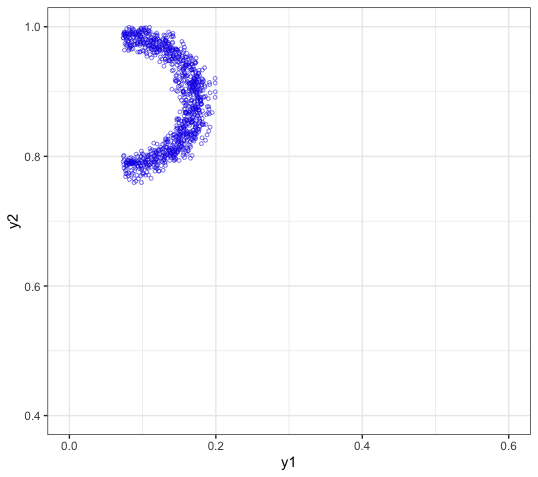
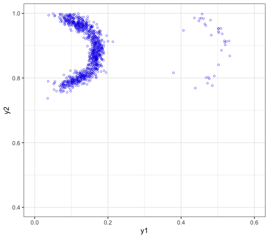
The GLLiM model is estimated using simulations $𝐘{}_N$. Selecting from $K=2$ to $50$, the smallest BIC was obtained for $K=49$. Figure 2 shows the different obtained samples. In this example, only the RW MH algorithm is tested as a MCMC scheme. We note that the uBSL variant from the BSL package exhibited a runtime error in this particular example and, as a result, was not used.

All methods identify the bimodality of the posterior distribution, but the BSL methods do not correctly recover the local structure of the two parts. In contrast, GLLiM-BSL provides a good representation of the posterior mass and moon structures. Among GLLiM-based procedures, the two moons were slightly better recovered with GLLiM-BSL than with the direct GLLiM posterior approximation. Table 1 shows the computing times obtained on a laptop (MacBook Pro, 2.4 GHz Quad-Core Intel Core i5) using the mentioned CRAN packages, and additional basic R code with no resorting to parallel computing. For the low dimensions of this example, i.e., $d=p=2$, the computing times were always less for GLLiM-based procedures, but not significantly so. However, the amortization nature of the GLLiM solution becomes an advantage in higher-dimensional problems, as seen in the following example.

This example was introduced in Forbes et al. (2022) and exhibits a posterior distribution whose mass is located on 4 hyperboloids, as illustrated in Figure 3 (a). The GLLiM estimator was used to produce an MoE with $K=38$ mixture components, as selected by BIC. The GLLiM-based likelihood was used with an RW MH algorithm to make comparisons with the standard BSL procedures. We also considered SS and G MH. In G MH, the variance of the GLLiM posterior was multiplied by 2 to avoid the proposal distribution being too narrow. The acceptance rate was 60% for G MH vs 16% for RW MH.

As depicted in Figure 3, although the posterior is far from being unimodal, some of the standard BSL variants (semiBSL and missBSL) succeed in capturing it satisfactorily compared to the previous example. This is likely due to the fact that the likelihood is simpler here, being a mixture of two Student distributions. Figure 3 shows the best results, obtained with GLLiM-BSL (c,d) and semiBSL (f). GLLiM approximations (Figure 3 (b,c,d)) appear to be better at capturing the hyperboloid branches, while some of the BSL variants (f,g,h), are more precise in the center with an obvious excess mass at the intersections of the branches. To complement this visual comparison, we also show the posterior marginals in Figure 4. The marginal plots allow us to better visualize the difference with standard BSL procedures. Refer to Figure 4 (f-j), which all show larger deviations from the truth, determined by numerical integration. Both true posterior marginals are the same due to symmetry in the model formulation and exhibit a non-smooth shape, which has also been double-checked using a long run of $3\times 10{}^5$ iterations of the SS algorithm; see Figure 4 (a). For GLLiM-BSL, among the three MCMC schemes, it appears that the SS version in Figure 4 (d) provides more satisfactory samples than the MH versions (c, e). The gain over the direct GLLiM posterior sample (b) is also clearer. Computing times are reported in Table 1. For the larger dimensional example ($d=10$), GLLiM methods take much less time than standard BSL, even when considering BIC and learning times.