Supplementary material: Summary statistics and discrepancy measures for approximate Bayesian computation via surrogate posteriors

Florence Forbes; Hien Duy Nguyen; TrungTin Nguyen; Julyan Arbel

S1 GLLiM for i.i.d. data

The GLLiM implementation of Deleforge et al. (2015) is adapted to account for the fact that for each parameters values, the observations may be available as $R$ i.i.d. realizations. The link to the setting where the covariance matrices of the direct model are block diagonal is explained. The resulting GLLiM-iid algorithm is detailed. This new procedure can also be useful when dealing with long stationary time series by cutting them into smaller series neglecting dependencies between the sub-series.

S1 .1 Likelihood and posterior approximations with Gaussian mixtures

The Gaussian Locally Linear Mapping (GLLiM) model of Deleforge et al. (2015) is first recalled but note that to match the notation in the manuscript, the notation of Deleforge et al. (2015) has been changed. GLLiM provides probability distributions selected in a family of mixture of Gaussian distributions. An attractive approach for modeling non linear relationships, between some parameters $𝜽 \in ℝ^{ℓ}$ and observations $𝐲 \in ℝ^{d}$ , is to use a mixture of linear models. We assume that each observed $𝐲$ is the noisy image of parameter $𝜽$ obtained from a $K$ -component mixture of affine transformations. This is modeled by introducing a latent variable $z \in {1, \dots, K}$ such that

𝐲

=

\sum_{k = 1}^{K} 1I_{{z = k}} (\tilde{𝑨}_{k} 𝜽 + \tilde{𝒃}_{k} + \tilde{ϵ}_{k})

(1)

where 1I is the indicator function, $\tilde{𝑨}_{k}$ a $d \times ℓ$ matrix and $\tilde{𝒃}_{k}$ a vector of $ℝ^{d}$ that define an affine transformation. Variable $\tilde{ϵ}_{k}$ corresponds to an error term which is assumed to be zero-mean and not correlated with $𝜽$ capturing both the observation noise and the reconstruction error due to the affine approximation. To make the affine transformations local, the latent variable $z$ should also depend on $𝜽$ .

For the posterior distribution $p (𝜽 | 𝐲)$ and the likelihood $p (𝐲 | 𝜽)$ to be easily derived, it is important to control the nature of the joint $p (𝐲, 𝜽)$ . Once a family of tractable joint distributions is chosen, we can look for one that is compatible with (1). In Deleforge et al. (2015) the GLLiM model is derived assuming that the joint distribution is a mixture of Gaussian distributions. Using a subscript $G$ to specify the model, it is assumed that $\tilde{ϵ}_{k} \sim 𝒩_{d} (𝟎, \tilde{𝚺}_{k})$ and that $𝜽$ is distributed as a mixture of $K$ Gaussian distributions specified by

	$p_{G} (𝜽 \| z = k)$	$=$	$𝒩_{ℓ} (𝜽; \tilde{𝒄}_{k}, \tilde{𝚪}_{k}),$		(2)
	$and p_{G} (z = k)$	$=$	$π_{k} .$		(3)

When informative, we specify the dimension of the Gaussian variable (e.g. $d$ ) in the notation $𝒩_{d}$ . The model parameters are then denoted by $\tilde{ϕ} = {π_{k}, \tilde{𝒄}_{k}, \tilde{𝚪}_{k}, \tilde{𝑨}_{k}, \tilde{𝒃}_{k}, \tilde{𝚺}_{k}}_{k = 1 : K} .$

One interesting property of such a parametric model is that both conditional distributions are available in closed form :

	$p_{G} (𝐲 \| 𝜽; \tilde{ϕ})$	$= \sum_{k = 1}^{K} \tilde{η}_{k} (𝜽) 𝒩_{d} (𝐲; \tilde{𝑨}_{k} 𝜽 + \tilde{𝒃}_{k}, \tilde{𝚺}_{k}) with \tilde{η}_{k} (𝜽) = \frac{π_{k} 𝒩_{ℓ} (𝜽; \tilde{𝒄}_{k}, \tilde{𝚪}_{k})}{\sum_{j = 1}^{K} π_{j} 𝒩_{ℓ} (𝜽; \tilde{𝒄}_{j}, \tilde{𝚪}_{j})}$		(4)
	$p_{G} (𝜽 \| 𝐲, ϕ)$	$= \sum_{k = 1}^{K} η_{k} (𝐲) 𝒩_{ℓ} (𝜽; 𝑨_{k} 𝐲 + 𝒃_{k}, 𝚺_{k}) with η_{k} (𝐲) = \frac{π_{k} 𝒩_{d} (𝐲; 𝒄_{k}, 𝚪_{k})}{\sum_{j = 1}^{K} π_{j} 𝒩_{d} (𝐲; 𝒄_{j}, 𝚪_{j})} .$		(5)

A different notation $ϕ$ is used in (5) but parameters $ϕ$ are easily deduced from $\tilde{ϕ}$ as follows (the $π_{k}$ ’s are unchanged):

$𝒄_{k} =$	$\tilde{𝑨}_{k} \tilde{𝒄}_{k} + \tilde{𝒃}_{k}, 𝚪_{k} = \tilde{𝚺}_{k} + \tilde{𝑨}_{k} \tilde{𝚪}_{k} \tilde{𝑨}_{k}^{⊤}$
$𝚺_{k} =$	$(\tilde{𝚪}_{k}^{- 1} + \tilde{𝑨}_{k}^{⊤} \tilde{𝚺}_{k}^{- 1} \tilde{𝑨}_{k})^{- 1}$	(6)
$𝑨_{k} =$	$𝚺_{k} \tilde{𝑨}_{k}^{⊤} \tilde{𝚺}_{k}^{- 1}, 𝒃_{k} = 𝚺_{k} (\tilde{𝚪}_{k}^{- 1} \tilde{𝒄}_{k} - \tilde{𝑨}_{k}^{⊤} \tilde{𝚺}_{k}^{- 1} \tilde{𝒃}_{k}) .$

The expressions above depend on the value of the parameters $\tilde{ϕ}$ that needs to be specified. In Deleforge et al. (2015), parameters $\tilde{ϕ}$ are estimated using a maximum likelihood principle with an EM algorithm applied to a learning set of $N$ couples $𝒟_{N} = {(𝜽_{n}, 𝐲_{n}), n \in [N]}$ . Once estimated, the parameters lead to an analytical expression of the form (5) denoted by $p_{G} (𝜽 | 𝐲; ϕ^{*}_{K, N})$ , which is a mixture of Gaussian distributions and can be seen as a parametric mapping from $𝐲$ values to the pdfs on $𝜽$ . $ϕ^{*}_{K, N}$ can be kept the same for all conditional distributions and does not need to be re-estimated for each new $𝜽$ or $𝐲$ to be inverted.

In practice when $d$ is much larger than $ℓ$ , it is more efficient to estimate $\tilde{ϕ}$ from the available data $𝒟_{N}$ to then deduce $ϕ^{*}_{K, N}$ and subsequently the conditional distribution of interest (5). The reason is that the size of $\tilde{ϕ}$ can be significantly reduced by choosing constraints on matrices $\tilde{𝚺}_{k}$ without oversimplifying the target conditional (5). The number of parameters depends on the exact variant learned but is in $𝒪 (d K ℓ)$ . Typically, diagonal covariance matrices $\tilde{𝚺}_{k}$ can be used with a drastic gain. More specifically for the case of diagonal covariances $\tilde{𝚺}_{k}$ , the number of parameters is $K - 1 + K (ℓ + ℓ (ℓ + 1) / 2 + d ℓ + 2 d)$ which for $K = 100$ , $ℓ = 4$ and $d = 10$ leads to 7499 parameters and to 61499 parameters if $d = 100$ . In addition to the diagonal case, other constraints are implemented in Deleforge et al. (2015), e.g. isotropic, full (no constraint), or equal across $k$ , $\tilde{𝚺}_{k}$ ’s. In particular, a good compromise between parsimonious and full covariance matrices can be obtained by combining the latter constraints with low rank matrices using the so-called Hybrid-GLLiM (eq. (20) in Deleforge et al. (2015)). All details are provided in Deleforge et al. (2015).

In this work, we aim at adapting the GLLiM model and inference to the case of i.i.d. observations. It requires the use of another type of constraint, not treated in Deleforge et al. (2015), that induces a block diagonal shape for the $\tilde{𝚺}_{k}$ ’s. In the next section we recall the main EM algorithm steps and explain how to modify them to account for this new constraint.

S1 .1.1 GLLiM model parameter estimation

The main updating steps are recalled below.

E-step.

The E-step consists in updating the assignments probabilities of each pair $(𝜽_{n}, 𝐲_{n})$ to each of the $K$ components, namely for each $k \in [K]$ and $n \in [N]$ ,

r_{n k}

\propto

π_{k} 𝒩_{d} (𝐲_{n}; \tilde{𝑨}_{k} 𝜽_{n} + \tilde{𝒃}_{k}, \tilde{𝚺}_{k}) 𝒩_{ℓ} (𝜽_{n}; \tilde{𝒄}_{k}, \tilde{𝚪}_{k}) .

(7)

M-step.

Denoting $r_{k} = \sum_{n = 1}^{N} r_{n k}$ , the M-step consists of updating the parameters and decomposes in 3 steps updating successively the $π_{k}$ ’s, the $\tilde{𝒄}_{k}, \tilde{𝚪}_{k}$ ’s and the $\tilde{𝑨}_{k}, \tilde{𝒃}_{k}, \tilde{𝚺}_{k}$ ’s.

$π_{k}$	$=$	$\frac{r_{k}}{N}$	(8)
$\tilde{𝒄}_{k}$	$=$	$\frac{1}{r_{k}} \sum_{n = 1}^{N} r_{n k} 𝜽_{n}$	(9)
$\tilde{𝚪}_{k}$	$=$	$\frac{1}{r_{k}} \sum_{n = 1}^{N} r_{n k} (𝜽_{n} - \tilde{𝒄}_{k}) (𝜽_{n} - \tilde{𝒄}_{k})^{T}$	(10)
$\tilde{𝑨}_{k}$	$=$	$𝐘_{k} 𝑻_{k}^{T} (𝑻_{k} 𝑻_{k}^{T})^{- 1}$	(11)
$\tilde{𝒃}_{k}$	$=$	$\bar{𝐲}_{k} - \tilde{𝑨}_{k} \tilde{𝒄}_{k}$	(12)
$\tilde{𝚺}_{k}$	$=$	$\frac{1}{r_{k}} \sum_{n = 1}^{N} r_{n k} (𝐲_{n} - \tilde{𝑨}_{k} 𝜽_{n} - \tilde{𝒃}_{k}) (𝐲_{n} - \tilde{𝑨}_{k} 𝜽_{n} - \tilde{𝒃}_{k})^{T} .$	(13)

The updating of $\tilde{𝑨}_{k}$ and $\tilde{𝒃}_{k}$ requires in addition the following quantities depending on the $r_{n k}$ ’s and the data set,

$\bar{𝐲}_{k}$	$=$	$\frac{1}{r_{k}} \sum_{n = 1}^{N} r_{n k} 𝐲_{n}$
$𝑻_{k}$	$=$	$\frac{1}{\sqrt{r_{k}}} [\sqrt{r_{1 k}} (𝜽_{1} - \tilde{𝒄}_{k}) \dots \sqrt{r_{N k}} (𝜽_{N} - \tilde{𝒄}_{k})]$
$𝐘_{k}$	$=$	$\frac{1}{\sqrt{r_{k}}} [\sqrt{r_{1 k}} (𝐲_{1} - \bar{𝐲}_{k}) \dots \sqrt{r_{N k}} (𝐲_{N} - \bar{𝐲}_{k})] .$

We now explain how these steps are modified in the i.i.d. case.

S1 .2 GLLiM-iid

S1 .2.1 Estimation with block constraints

In this section, we consider the case where for a given parameter $𝜽$ , a sample of $R$ observations ${𝐲^{1}, \dots, 𝐲^{R}}$ is generated independently from the likelihood $p (𝐲 | 𝜽)$ . Therefore, we have $p (𝐲^{1}, \dots, 𝐲^{R} | 𝜽) = \prod_{r = 1}^{R} p (𝐲^{r} | 𝜽)$ and we are interested in computing the posterior $p (𝜽 | 𝐲^{1}, \dots, 𝐲^{R})$ . If $R = 1$ we recover the setting handled by standard GLLiM. If $R > 1$ , we define a new model and procedure referred to as GLLiM-iid as follows. Note that a key point for our GLLiM-ABC procedure is that the posterior $p (𝜽 | 𝐲^{1}, \dots, 𝐲^{R})$ still be approximated by a mixture.

Considering the joint $p (𝐲^{1}, \dots, 𝐲^{R}, 𝜽) = p (𝐲^{1}, \dots, 𝐲^{R} | 𝜽) p (𝜽) = p (𝜽) \prod_{r = 1}^{R} p (𝐲^{r} | 𝜽)$ , we approximate it by using for $p (𝜽)$ the same mixture model as in standard GLLiM in (2), (3) and for $p (𝐲^{1}, \dots, 𝐲^{R} | 𝜽)$ we assume also a mixture form (we use a different notation $q_{G}$ to emphasize that it is a particular case of $p_{G}$ :

q_{G} (𝐲^{1}, \dots, 𝐲^{R} | 𝜽)

=

\sum_{k = 1}^{K} (\tilde{η}_{k} (𝜽) \prod_{r = 1}^{R} 𝒩_{d} (𝐲_{r}; \tilde{𝑨}_{k} 𝜽 + \tilde{𝒃}_{k}, \tilde{𝚺}_{k})) .

(14)

The product in the rhs corresponds to a $d R$ -dimensional Gaussian density with $R$ independent and identical components all of dimension $d$ . This corresponds to a specific constrained GLLiM model where the dimension $d$ has changed to $d R$ and $ℓ$ remains the same. We can then compute the MLE via EM for this constrained parameters setting. The expressions for $π_{k}, \tilde{𝒄}_{k}, \tilde{𝚪}_{k}$ remain the same, while the expressions for $\tilde{𝑨}_{k}, \tilde{𝒃}_{k}, \tilde{𝚺}_{k}$ are changed using $N \times R$ data points instead of just $N$ . All expressions use a formula for the $r_{n k}$ (the responsibilities) that needs to be modified. This EM algorithm is detailed below.

Observations are now made of $R$ i.i.d. vectors of size $d$ and are denoted by $\hat{𝐲}$ with $\hat{𝐲} = [𝐲^{1}, \dots, 𝐲^{R}]^{T}$ . The same expressions (4) and (5) can be used with now parameters $\tilde{ϕ}$ denoted by $\hat{ϕ}$ and $\hat{𝚺}_{k}$ of dimension $d R \times d R$ , $\hat{𝑨}_{k}$ of dimension $d R \times ℓ$ , $\hat{𝒃}_{k}$ of length $d R$ , while the dimensions of $\hat{𝒄}_{k}$ and $\hat{𝚪}_{k}$ do not change. Inference could be carried out with the EM described in Section S1 .1.1 with these new dimensions but that would not take into account that the $𝐲^{r}$ ’s are i.i.d.. Thus, we propose to add the following constraints, assuming that $\hat{𝚺}_{k}$ is a block diagonal matrix made of $R$ blocks all equal to $d \times d$ $\tilde{𝚺}_{k}$ , $\hat{𝑨}_{k}$ is made of $R$ blocks all equal to $\tilde{𝑨}_{k}$ of size $d \times ℓ$ and $\hat{𝒃}_{k}$ is a vector of $R$ concatenated vectors all equal to a vector $\tilde{𝒃}_{k}$ of length $d$ . Note that this is similar to consider a GLLiM model with an additional constraint on the $\hat{𝚺}_{k}$ ’s, namely a block diagonal structure except that in this later case no constraint would be assumed on $\hat{𝑨}_{k}$ and $\hat{𝒃}_{k}$ .

It follows that $q_{G} (\hat{𝐲} | 𝜽, z = k) = \prod_{r = 1}^{R} q_{G} (𝐲^{r} | 𝜽, z = k)$ . As already mentioned, this is not modelling the likelihood as a product but it consists in assuming instead that given $z = k$ , so region-wise, the $𝐲^{r}$ ’s are i.i.d.

The E-step becomes,

r_{n k}

\propto

π_{k} 𝒩_{ℓ} (𝜽_{n}; \tilde{𝒄}_{k}, \tilde{𝚪}_{k}) \prod_{r = 1}^{R} 𝒩_{d} (𝐲^{r}_{n}; \tilde{𝑨}_{k} 𝜽_{n} + \tilde{𝒃}_{k}, \tilde{𝚺}_{k}) .

(15)

For the M-step, the expressions for $r_{k}, π_{k}, \tilde{𝒄}_{k}, \tilde{𝚪}_{k}$ are the same as before (8-10). The rest of the parameters is modified as follows,

$\tilde{𝑨}_{k}$	$=$	$(\frac{1}{R} \sum_{r = 1}^{R} 𝐘^{r}_{k}) 𝑻_{k}^{T} (𝑻_{k} 𝑻_{k}^{T})^{- 1}$	(16)
$\tilde{𝒃}_{k}$	$=$	$\frac{1}{R} \sum_{r = 1}^{R} \bar{𝐲}^{r}_{k} - \tilde{𝑨}_{k} \tilde{𝒄}_{k}$	(17)
$\tilde{𝚺}_{k}$	$=$	$\frac{1}{R} \sum_{r = 1}^{R} (\frac{1}{r_{k}} \sum_{n = 1}^{N} r_{n k} (𝐲^{r}_{n} - \tilde{𝑨}_{k} 𝜽_{n} - \tilde{𝒃}_{k}) (𝐲^{r}_{n} - \tilde{𝑨}_{k} 𝜽_{n} - \tilde{𝒃}_{k})^{T})$	(18)

with

$\bar{𝐲}^{r}_{k}$	$=$	$\frac{1}{r_{k}} \sum_{n = 1}^{N} r_{n k} 𝐲^{r}_{n}$
$\bar{𝐲}_{k}$	$=$	$\frac{1}{R} \sum_{r = 1}^{R} \bar{𝐲}^{r}_{k}$
$𝑻_{k}$	$=$	$\frac{1}{\sqrt{r_{k}}} [\sqrt{r_{1 k}} (𝜽_{1} - \tilde{𝒄}_{k}) \dots \sqrt{r_{N k}} (𝜽_{N} - \tilde{𝒄}_{k})]$
$𝐘_{k}^{r}$	$=$	$\frac{1}{\sqrt{r_{k}}} [\sqrt{r_{1 k}} (𝐲^{r}_{1} - \bar{𝐲}_{k}) \dots \sqrt{r_{N k}} (𝐲^{r}_{N} - \bar{𝐲}_{k})] .$

Note the use of $\bar{𝐲}_{k}$ and not $\bar{𝐲}^{r}_{k}$ in the last expression.

S1 .2.2 Surrogate posteriors in the i.i.d. case

The conditional distributions expressions follow from applying the constraint in (4) and (5). Denoting by $\hat{𝐲}$ the column vector made of the concatenated $𝐲^{1}, \dots, 𝐲^{R}$ ,

q_{G} (𝜽 | 𝐲^{1}, \dots, 𝐲^{R})

=

\sum_{k = 1}^{K} η_{k}^{*} (𝐲^{1}, \dots, 𝐲^{R}) 𝒩_{ℓ} (𝜽; \hat{𝑨}_{k}^{*} \hat{𝐲} + \hat{𝒃}_{k}^{*}, \hat{𝚺}^{*}_{k}),

(19)

where the various parameters and expressions involved are specified below with respect to $\tilde{ϕ}$ estimated via the EM algorithm described before:

$\hat{𝚺}^{*}_{k}$	$=$	$(\tilde{𝚪}_{k}^{- 1} + R \tilde{𝑨}_{k}^{T} \tilde{𝚺}_{k}^{- 1} \tilde{𝑨}_{k})^{- 1}$	(20)
$\hat{𝑨}_{k}^{} \hat{𝐲} + \hat{𝒃}_{k}^{}$	$=$	$\hat{𝚺}^{*}_{k} (\tilde{𝑨}_{k}^{T} \tilde{𝚺}_{k}^{- 1} (\sum_{r = 1}^{R} 𝐲^{r}) + \tilde{𝚪}_{k}^{- 1} \tilde{𝒄}_{k} - R \tilde{𝑨}_{k}^{T} \tilde{𝚺}_{k}^{- 1} \tilde{𝒃}_{k})$	(21)
$η_{k}^{*} (𝐲^{1}, \dots, 𝐲^{R})$	$\propto$	$π_{k} 𝒩_{d R} (\tilde{𝐲}; 𝒎_{k}, 𝑽_{k}),$	(22)

where $𝒎_{k}$ is a vector made of $R$ concatenated $d$ -dimensional vectors all equal to $\tilde{𝑨}_{k} \tilde{𝒄}_{k} + \tilde{𝒃}_{k}$ and $𝑽_{k}$ is a matrix made of $R \times R$ blocks of size $d \times d$ which is the sum of a block diagonal matrix with all diagonal blocks equal to $\tilde{𝚺}_{k}$ and of a matrix made of constant blocks all equal to $\tilde{𝑨}_{k} \tilde{𝚪}_{k} \tilde{𝑨}_{k}^{T}$ .

As $d R$ can be large, e.g. 1000, the computation of $η_{k}^{*}$ can be numerically problematic. However the quadratic forms and the determinants involved can simplify using the Woodbury formula and the matrix determinant lemma. Let $S_{k} = (\hat{𝐲} - 𝒎_{k})^{T} 𝑽^{- 1}_{k} (\hat{𝐲} - 𝒎_{k})$ , the Woodbury formula leads to:

	$S_{k}$	$=$	$\sum_{r = 1}^{R} (𝐲^{r} - \tilde{𝑨}_{k} \tilde{𝒄}_{k} - \tilde{𝒃}_{k})^{T} \tilde{𝚺}_{k}^{- 1} (𝐲^{r} - \tilde{𝑨}_{k} \tilde{𝒄}_{k} - \tilde{𝒃}_{k})$
			$- (\sum_{r = 1}^{R} 𝐲^{r} - R \tilde{𝑨}_{k} \tilde{𝒄}_{k} - R \tilde{𝒃}_{k})^{T} (\tilde{𝚺}_{k}^{- 1} \tilde{𝑨}_{k} \hat{𝚺}_{k}^{*} \tilde{𝑨}^{T}_{k} \tilde{𝚺}_{k}^{- 1}) (\sum_{r = 1}^{R} 𝐲^{r} - R \tilde{𝑨}_{k} \tilde{𝒄}_{k} - R \tilde{𝒃}_{k}) .$

Similarly for the determinant of $𝑽_{k}$ we get:

| 𝑽_{k} | = | \tilde{𝚺}_{k} |^{R} \times | 𝑰 + R \tilde{𝚪}_{k}^{1 / 2} \tilde{𝑨}_{k}^{T} \tilde{𝚺}_{k}^{- 1} \tilde{𝑨}_{k} \tilde{𝚪}_{k}^{1 / 2} |,

or equivalently

| 𝑽_{k} | = | \tilde{𝚺}_{k} |^{R} \times | 𝑰 + R \tilde{𝚪}_{k} \tilde{𝑨}_{k}^{T} \tilde{𝚺}_{k}^{- 1} \tilde{𝑨}_{k} | .

So that

\log η_{k}^{*} = \log π_{k} - 0.5 S_{k} - 0.5 \log | 𝑽_{k} | + C .

The estimated $\tilde{ϕ}_{R}$ parameters can then be used to specify (19).

S2 Distances between Gaussian mixtures

S2 .1 Optimal transport-based distance between Gaussian mixtures

Delon and Desolneux (2020); Chen et al. (2019) have introduced a distance specifically designed for Gaussian mixtures based on the Wasserstein distance. In an optimal transport context, by restricting the possible coupling measures (i.e., the optimal transport plan) to a Gaussian mixture, they propose a discrete formulation for this distance. This makes it tractable and suitable for high dimensional problems, while in general using the standard Wasserstein distance between mixtures is problematic. Delon and Desolneux (2020) refer to the proposed new distance as MW₂, for Mixture Wasserstein.

The MW₂ definition makes first use of the tractability of the Wasserstein distance between two Gaussians for a quadratic cost. The standard quadratic cost Wasserstein distance between two Gaussian pdfs $g_{1} (\cdot) = 𝒩 (\cdot; 𝝁_{1}, 𝚺_{1})$ and $g_{2} (\cdot) = 𝒩 (\cdot; 𝝁_{2}, 𝚺_{2})$ is (see Delon and Desolneux 2020),

W_{2}^{2} (g_{1}, g_{2}) = ∥ 𝝁_{1} - 𝝁_{2} ∥_{2}^{2} + trace (𝚺_{1} + 𝚺_{2} - 2 (𝚺_{1}^{1 / 2} 𝚺_{2} 𝚺_{1}^{1 / 2})^{1 / 2}) .

Section 4 of Delon and Desolneux (2020) shows that the MW₂ distance between two mixtures can be computed by solving the following discrete optimization problem. Let $f_{1} = \sum_{k = 1}^{K_{1}} π_{1 k} g_{1 k}$ and by $f_{2} = \sum_{k = 1}^{K_{2}} π_{2 k} g_{2 k}$ be two Gaussian mixtures. Then,

MW_{2}^{2} (f_{1}, f_{2})

= \min_{𝐰 \in Π (π_{1}, π_{2})} \sum_{k, l} w_{k l} W_{2}^{2} (g_{1 k}, g_{2 l}),

(23)

where $π_{1}$ and $π_{2}$ are the discrete distributions on the simplex defined by the respective weights of the mixtures and $Π (π_{1}, π_{2})$ is the set of discrete joint distributions $𝐰 = (w_{k l}, k \in [K_{1}], l \in [K_{2}])$ , whose marginals are $π_{1}$ and $π_{2}$ . Finding the minimizer $𝐰^{*}$ of (23) boils down to solving a simple discrete optimal transport problem, where the entries of the $K_{1} \times K_{2}$ dimensional cost matrix are the $W_{2}^{2} (g_{1 k}, g_{2 l})$ quantities.

As implicitly suggested above, MW₂ is indeed a distance on the space of Gaussian mixtures; see Delon and Desolneux (2020). In particular, for two Gaussian mixtures $f_{1}$ and $f_{2}$ , MW₂ satisfies the equality property according to which $MW 2 (f_{1}, f_{2}) = 0$ implies that $f_{1} = f_{2}$ . In our experiments, the MW₂ distances were computed using the transport R package (Schuhmacher et al., 2020).

S2 .2 L₂ distance between Gaussian mixtures

The L₂ distance between two square-integrable distributions $f_{1}$ and $f_{2}$ is $L_{2}^{2} (f_{1}, f_{2}) = \int (f_{1} (𝐱) - f_{2} (𝐱))^{2} d 𝐱$ . The L₂ distance between two Gaussian mixtures is also closed form. Denote by $f_{1} = \sum_{k = 1}^{K_{1}} π_{1 k} g_{1 k}$ and $f_{2} = \sum_{k = 1}^{K_{2}} π_{2 k} g_{2 k}$ two Gaussian mixtures,

L_{2}^{2} (f_{1}, f_{2})

= \sum_{k, l} π_{1 k} π_{1 l} ⟨ g_{1 k}, g_{1 l} ⟩ + \sum_{k, l} π_{2 k} π_{2 l} ⟨ g_{2 k}, g_{2 l} ⟩ - 2 \sum_{k, l} π_{1 k} π_{2 l} ⟨ g_{1 k}, g_{2 l} ⟩,

(24)

where $⟨ \cdot, \cdot ⟩$ denotes the L₂ scalar product, which is closed form for two Gaussian distributions $g_{1}$ and $g_{2}$ and given by $⟨ g_{1}, g_{2} ⟩ = 𝒩 (𝝁_{1}; 𝝁_{2}, 𝚺_{1} + 𝚺_{2})$ . The L₂ distance can be evaluated in $𝒪 (K_{1} K_{2})$ time. We do not discuss the different properties of the various possible distances but the distance choice has a potential impact on the associated GLLiM-D-ABC procedure. This impact is illustrated in the experimental Section S4.

S3 Proofs

S3 .1 Proof of Theorem 1

We follow steps similar to the proof of Proposition 2 in Bernton et al. (2019). The ABC quasi-posterior can be written as

q_{ϵ} (𝜽 ∣ 𝐲)

= \int_{𝒴} K_{ϵ} (𝐳; 𝐲) π (𝜽 ∣ 𝐳) d 𝐳,

where $K_{ϵ} (𝐳; 𝐲) \propto 𝟏_{{D (π (\cdot ∣ 𝐲), π (\cdot ∣ 𝐳))) \leq ϵ}} π (𝐳)$ denotes the density evaluated at some $𝐳$ of the prior truncated to $A_{ϵ}$ . $K_{ϵ} (\cdot; 𝐲)$ is a probability density function (pdf) in $𝐳 \in 𝒴$ with compact support $A_{ϵ} \subset 𝒴$ by definition of $A_{ϵ}$ and (A4). It follows that

	$\| q_{ϵ} (𝜽 ∣ 𝐲) - π (𝜽 ∣ 𝐲) \|$	$\leq \int_{𝒴} K_{ϵ} (𝐳; 𝐲) \| π (𝜽 ∣ 𝐳) - π (𝜽 ∣ 𝐲) \| d 𝐳$
		$\leq sup_{𝐳 \in A_{ϵ}} \| π (𝜽 ∣ 𝐳) - π (𝜽 ∣ 𝐲) \|$
		$= \| π (𝜽 ∣ 𝐳_{ϵ}) - π (𝜽 ∣ 𝐲) \|,$

for some $𝐳_{ϵ} \in A_{ϵ}$ , where the second inequality is due to the fact that $K_{ϵ} (\cdot; 𝐲)$ is a pdf, and the last equality is due to (A1) and the compacity of $A_{ϵ}$ .

Since for each $ϵ > 0$ , $𝐳_{ϵ} \in A_{ϵ}$ , we have $lim_{ϵ \to 0} 𝐳_{ϵ} \in A_{0}$ , where $A_{0} = ⋂_{ϵ \in ℚ_{+}} A_{ϵ}$ . Then, using that by continuity of $D$ , $A_{0} = {𝐳 \in 𝒴 : D (π (\cdot ∣ 𝐳), π (\cdot ∣ 𝐲)) = 0}$ , it follows from the equality property of $D$ , that $A_{0} = {𝐳 \in 𝒴 : π (\cdot ∣ 𝐳) = π (\cdot ∣ 𝐲)}$ . Taking the limit $ϵ \to 0$ yields

| π (𝜽 ∣ 𝐳_{ϵ}) - π (𝜽 ∣ 𝐲) | \to | π (𝜽 ∣ 𝐲) - π (𝜽 ∣ 𝐲) | = 0

and hence $| q_{ϵ} (𝜽 ∣ 𝐲) - π (𝜽 ∣ 𝐲) | \to 0$ , for each $θ \in Θ$ .

By (A2), we have

	$sup_{𝜽 \in Θ} q_{ϵ} (𝜽 ∣ 𝐲)$	$= sup_{𝜽 \in Θ} \int_{𝒴} K_{ϵ} (𝐳; 𝐲) π (𝜽 ∣ 𝐳) d 𝐳$
		$\leq sup_{𝜽 \in Θ} sup_{𝐳 \in A_{γ}} π (𝜽 ∣ 𝐳) < \infty,$

for some $γ$ , so that $ϵ \leq γ$ . Finally, by the bounded convergence theorem, we have

lim_{ϵ \to 0} \int_{Θ} | q_{ϵ} (𝜽 ∣ 𝐲) - π (𝜽 ∣ 𝐲) | d 𝜽 = lim_{ϵ \to 0} ∥ q_{ϵ} (\cdot ∣ 𝐲) - π (\cdot ∣ 𝐲) ∥_{1} = 0 .

S3 .2 Proof of Theorem 2

We now provide a detailed proof of Theorem 2. Given any $α > 0, β > 0$ , we claim that

lim_{ϵ \to 0, K \to \infty, N \to \infty} \Pr (λ ({𝐲 \in 𝒴 : D_{H}^{2} (q_{ϵ}^{K, N} (\cdot ∣ 𝐲), π (\cdot ∣ 𝐲)) \geq β}) \leq α) = 1;

or equivalently, for any $α > 0, β > 0, γ > 0$ , we wish to find $ϵ (α, β, γ) > 0$ , $K (α, β, γ) \in ℕ^{*}$ , and $N (α, β, γ) \in ℕ^{*}$ so that for all $ϵ < ϵ (α, β, γ), K \geq K (α, β, γ), N \geq N (α, β, γ)$ :

\Pr (λ ({𝐲 \in 𝒴 : D_{H}^{2} (q_{ϵ}^{K, N} (\cdot ∣ 𝐲), π (\cdot ∣ 𝐲)) \geq β}) > α) \leq γ .

(25)

To prove (25), we first recall that we can rewrite $q_{ϵ}^{K, N}$ as follows, for all $𝜽 \in Θ, 𝐲 \in 𝒴$ ,

	$q_{ϵ}^{K, N} (𝜽 ∣ 𝐲)$	$= \int_{𝒴} K^{K, N}_{ϵ} (𝐳; 𝐲) π (𝜽 ∣ 𝐳) d 𝐳,$
	$K^{K, N}_{ϵ} (𝐳; 𝐲)$	$= \frac{𝟏_{A^{K, N}_{ϵ, 𝐲}} (𝐳) π (𝐳)}{\int_{𝒴} 𝟏_{A^{K, N}_{ϵ, 𝐲}} (𝐳) π (𝐳) d 𝐳},$		(26)

where $K^{K, N}_{ϵ} (\cdot; 𝐲)$ is a pdf on $𝐳 \in 𝒴$ with compact support $A^{K, N}_{ϵ, 𝐲} \subset 𝒴$ by definition of $A^{K, N}_{ϵ, 𝐲}$ and (B4).

The Hellinger distance $D_{H}$ , between two densities $f$ and $g$ in appropriate spaces, is related to the L₁ distance $D_{1}$ as follows, see Zeevi and Meir (1997, Lemma 1),

(\frac{1}{2} D_{1} (f, g))^{2} \leq D^{2}_{H} (f, g) \leq D_{1} (f, g) .

(27)

Applying successively the right-hand-side of (27), the definition of $q_{ϵ}^{K, N}$ and the fact that $K^{K, N}_{ϵ} (\cdot; 𝐲)$ is a pdf, we can write

	$D_{H}^{2} (q_{ϵ}^{K, N} (\cdot ∣ 𝐲), π (\cdot ∣ 𝐲))$	$\leq D_{1} (q_{ϵ}^{K, N} (\cdot ∣ 𝐲), π (\cdot ∣ 𝐲))$
		$= \int_{Θ} \| q_{ϵ}^{K, N} (𝜽 ∣ 𝐲) - π (𝜽 ∣ 𝐲) \| d λ (𝜽)$
		$\leq \int_{Θ} \int_{𝒴} K_{ϵ}^{K, N} (𝐳; 𝐲) \| π (𝜽 ∣ 𝐳) - π (𝜽 ∣ 𝐲) \| d λ (𝐳) d λ (𝜽)$
		$= \int_{𝒴} K_{ϵ}^{K, N} (𝐳; 𝐲) \int_{Θ} \| π (𝜽 ∣ 𝐳) - π (𝜽 ∣ 𝐲) \| d λ (𝜽) d λ (𝐳)$
		$\leq sup_{𝐳 \in A_{ϵ, 𝐲}^{K, N}} \int_{Θ} \| π (𝜽 ∣ 𝐳) - π (𝜽 ∣ 𝐲) \| d λ (𝜽) .$

Then using Makarov and Podkorytov (2013, Corollary 7.1.3) and the continuity of $π (\cdot ∣ \cdot)$ (B2), it follows that $𝐳 \mapsto D_{1} (π (\cdot ∣ 𝐳), π (\cdot ∣ 𝐲))$ is a continuous function for every $𝐲 \in 𝒴$ . As $A_{ϵ, 𝐲}^{K, N}$ is compact, since

𝐳_{ϵ, 𝐲}^{K, N} \in B_{ϵ, 𝐲}^{K, N} = a r g m a x_{𝐳 \in A_{ϵ, 𝐲}^{K, N}} D_{1} (π (\cdot ∣ 𝐳), π (\cdot ∣ 𝐲)),

sup_{𝐳 \in A_{ϵ, 𝐲}^{K, N}} D_{1} (π (\cdot ∣ 𝐳), π (\cdot ∣ 𝐲))

= D_{1} (π (\cdot ∣ 𝐳_{ϵ, 𝐲}^{K, N}), π (\cdot ∣ 𝐲)),

and using the left-hand-side of (27), we finally get that

D_{H}^{2} (q_{ϵ}^{K, N} (\cdot ∣ 𝐲), π (\cdot ∣ 𝐲))

\leq 2 D_{H} (π (\cdot ∣ 𝐳_{ϵ, 𝐲}^{K, N}), π (\cdot ∣ 𝐲)) .

(28)

Consider the limit point $𝐳^{K, N}_{0, 𝐲}$ defined as $𝐳^{K, N}_{0, 𝐲} = lim_{ϵ \to 0} 𝐳^{K, N}_{ϵ, 𝐲} .$ Since for each $ϵ > 0$ , $𝐳^{K, N}_{ϵ, 𝐲} \in A^{K, N}_{ϵ, 𝐲}$ then $𝐳^{K, N}_{0, 𝐲} \in A^{K, N}_{0, 𝐲}$ , where $A^{K, N}_{0, 𝐲} = ⋂_{ϵ \in ℚ_{+}} A^{K, N}_{ϵ, 𝐲}$ . By continuity of $D$ , $A^{K, N}_{0, 𝐲} = {𝐳 \in 𝒴 : D (p^{K, N} (\cdot ∣ 𝐳), p^{K, N} (\cdot ∣ 𝐲)) = 0}$ and $A^{K, N}_{0, 𝐲} = {𝐳 \in 𝒴 : p^{K, N} (\cdot ∣ 𝐳) = p^{K, N} (\cdot ∣ 𝐲)}$ , using (B3).

The distance on the right-hand side of (28) can then be bounded by three terms using the triangle inequality for the Hellinger distance $D_{H}$ ,

	$D_{H} (π (\cdot ∣ 𝐳_{ϵ, 𝐲}^{K, N}), π (\cdot ∣ 𝐲))$	$\leq D_{H} (π (\cdot ∣ 𝐳_{ϵ, 𝐲}^{K, N}), π (\cdot ∣ 𝐳_{0, 𝐲}^{K, N})) + D_{H} (π (\cdot ∣ 𝐳_{0, 𝐲}^{K, N}), p^{K, N} (\cdot ∣ 𝐲))$
		$+ D_{H} (p^{K, N} (\cdot ∣ 𝐲), π (\cdot ∣ 𝐲)) .$		(29)

The first term on the right-hand side can be made close to 0 as $ϵ$ goes to 0 independently of $K$ and $N$ . The two other terms are of the same nature as the definition of $𝐳^{K, N}_{0, 𝐲}$ yields $p^{K, N} (\cdot ∣ 𝐲) = p^{K, N} (\cdot ∣ 𝐳^{K, N}_{0, 𝐲}) .$

Therefore, we first prove that $lim_{ϵ \to 0} D^{2}_{H} (π (\cdot ∣ 𝐳^{K, N}_{ϵ, 𝐲}), π (\cdot ∣ 𝐳^{K, N}_{0, 𝐲})) = 0$ pointwise i.e. for each $𝐲$ . Indeed, since $π (\cdot ∣ \cdot)$ is a uniformly continuous function in $(𝜽, 𝐲)$ , given any $𝐲 \in 𝒴$ , $α_{1} > 0$ , there exists $δ (α_{1}) > 0$ such that for all $𝐳^{K, N}_{0, 𝐲} \in A^{K, N}_{0, 𝐲} \subset 𝒴$ ,

sup_{𝜽 \in Θ} | π (𝜽 ∣ 𝐳) - π (𝜽 ∣ 𝐳^{K, N}_{0, 𝐲}) |

\leq α_{1}, \forall 𝐳 \in 𝒴, | 𝐳 - 𝐳^{K, N}_{0, 𝐲} | < δ (α_{1}) .

(30)

Furthermore, since $Θ$ is a subset of a compact set, $λ (Θ) < \infty$ . Hence, by using the fact that $lim_{ϵ \to 0} 𝐳^{K, N}_{ϵ, 𝐲} = 𝐳^{K, N}_{0, 𝐲} \in A^{K, N}_{0, 𝐲}$ pointwise with respect to $𝐲$ and choosing $𝐳 = 𝐳^{K, N}_{ϵ, 𝐲}$ in (30), we obtain that given any $𝐲 \in 𝒴$ , and $α_{1} > 0$ , there exists $δ (α_{1}) > 0$ , and $ϵ (δ (α_{1})) > 0$ such that $\forall 0 < ϵ < ϵ (δ (α_{1}))$ , $| 𝐳^{K, N}_{ϵ, 𝐲} - 𝐳^{K, N}_{0, 𝐲} | < δ (α_{1})$ . Using (27) and (30), it follows for any $ϵ$ such that $0 < ϵ < ϵ (δ (α_{1}))$ ,

$D^{2}_{H} (π (\cdot ∣ 𝐳^{K, N}_{ϵ, 𝐲}), π (\cdot ∣ 𝐳^{K, N}_{0, 𝐲}))$	$\leq D_{1} (π (\cdot ∣ 𝐳^{K, N}_{ϵ, 𝐲}), π (\cdot ∣ 𝐳^{K, N}_{0, 𝐲}))$
	$\leq sup_{𝜽 \in Θ} \| π (𝜽 ∣ 𝐳^{K, N}_{ϵ, 𝐲}) - π (𝜽 ∣ 𝐳^{K, N}_{0, 𝐲}) \| λ (Θ)$
	$\leq α_{1} λ (Θ) .$	(31)

Such convergence also holds in measure $λ$ . Given any $α_{1} > 0$ , $β_{1} > 0$ , there exists $ϵ (α_{1}, β_{1}) > 0$ such that for any $0 < ϵ < ϵ (α_{1}, β_{1})$ ,

λ ({𝐲 \in 𝒴 : D^{2}_{H} (π (\cdot ∣ 𝐳^{K, N}_{ϵ, 𝐲}), π (\cdot ∣ 𝐳^{K, N}_{0, 𝐲})) \geq β_{1}}) \leq α_{1} .

(32)

Then, since (32) is true whatever the value of ${(𝜽_{n}, 𝐲_{n}), n \in [N]}$ , sampled from the joint $π (\cdot, \cdot)$ , it also holds, in probability with respect to the data set, that

\Pr (λ ({𝐲 \in 𝒴 : D^{2}_{H} (π (\cdot ∣ 𝐳^{K, N}_{ϵ, 𝐲}), π (\cdot ∣ 𝐳^{K, N}_{0, 𝐲})) \geq β_{1}}) > α_{1}) = 0 .

(33)

Next, we prove that $D^{2}_{H} (π (\cdot ∣ 𝐳^{K, N}_{0, 𝐲}), p^{K, N} (\cdot ∣ 𝐲))$ , equal to $D^{2}_{H} (π (\cdot ∣ 𝐳^{K, N}_{0, 𝐲}), p^{K, N} (\cdot ∣ 𝐳^{K, N}_{0, 𝐲}))$ , and $D^{2}_{H} (p^{K, N} (\cdot ∣ 𝐲), π (\cdot ∣ 𝐲))$ both converge to $0$ in measure $λ$ , with respect to $𝐲$ and in probability with respect to the sample ${(𝜽_{n}, 𝐲_{n}), n \in [N]}$ .

We first focus on $D^{2}_{H} (p^{K, N} (\cdot ∣ 𝐲), π (\cdot ∣ 𝐲))$ . Using the monotonicity of the Lebesgue integral and a result from Tsybakov (2008, Lemma 2.4) indicating that the squared Hellinger distance can be bounded by the Kullback–Leibler (KL) divergence, it follows that

\int_{𝒴} D^{2}_{H} (p^{K, N} (\cdot ∣ 𝐲), π (\cdot ∣ 𝐲)) d λ (𝐲)

\leq \int_{𝒴} K L (π (\cdot ∣ 𝐲), p^{K, N} (\cdot ∣ 𝐲)) d λ (𝐲) .

Then since $π (𝐲) \geq a λ (Θ)$

	$\int_{𝒴} K L (π (\cdot ∣ 𝐲), p^{K, N} (\cdot ∣ 𝐲)) d λ (𝐲)$	$\leq \frac{1}{a λ (Θ)} \int_{𝒴} π (𝐲) K L (π (\cdot ∣ 𝐲), p^{K, N} (\cdot ∣ 𝐲)) d λ (𝐲)$
		$\leq \frac{1}{a λ (Θ)} K L (π, p^{K, N}),$		(34)

where in the last right-hand side, the Kullback–Leibler divergence is on the joint densities $π$ and $p^{K, N}$ and the inequality is coming from a standard relationship between Kullback–Leibler divergences between joint and conditional distributions, i.e.

K L (π, p^{K, N}) = \int_{𝒴} π (𝐲) K L (π (\cdot ∣ 𝐲), p^{K, N} (\cdot ∣ 𝐲)) d λ (𝐲) + \int_{𝒴} π (𝐲) \log (\frac{π (𝐲)}{p^{K, N} (𝐲)}) d λ (𝐲),

with the last integral being a positive Kullback–Leibler divergence. Using Corollary 2.2 in Rakhlin et al. (2005) (see details in Section S3 .3.1), we can show that $K L (π, p^{K, N})$ tends to 0 in probability as $K$ and $N$ tends to infinity. It follows that $D^{2}_{H} (p^{K, N} (\cdot ∣ 𝐲), π (\cdot ∣ 𝐲))$ converges to $0$ in L₁ distance with respect to $𝐲$ . Using Tao (2011, 1.5. Modes of convergence), $D^{2}_{H} (p^{K, N} (\cdot ∣ 𝐲), π (\cdot ∣ 𝐲))$ also converges to $0$ in measure $λ$ with respect to $𝐲$ , and in probability with respect to the sample ${(𝜽_{n}, 𝐲_{n}), n \in [N]}$ as $K \to \infty, N \to \infty$ .

That is, given any $α_{2} > 0$ , $β_{2} > 0$ , $γ_{2} > 0$ , there exists $K (α_{2}, β_{2}, γ_{2}) \in ℕ^{*}$ , $N (α_{2}, β_{2}, γ_{2}) \in ℕ^{*}$ such that for any $K \geq K (α_{2}, β_{2}, γ_{2})$ , $N \geq N (α_{2}, β_{2}, γ_{2})$ ,

\Pr (λ ({𝐲 \in 𝒴, D^{2}_{H} (p^{K, N} (\cdot ∣ 𝐲), π (\cdot ∣ 𝐲)) \geq β_{2}}) > α_{2}) \leq γ_{2} .

(35)

To show that the same as (35) also holds when replacing $𝐲$ by $𝐳^{K, N}_{0, 𝐲}$ in $D^{2}_{H}$ , we need to show some measurability property with respect to $λ$ . Lemma 2, together with its proof in Subsection S3 .3.2, guaranties first that the map $𝐲 \mapsto 𝐳^{K, N}_{0} (𝐲) = 𝐳^{K, N}_{0, 𝐲}$ is measurable. Since $𝐲 \mapsto D^{2}_{H} (p^{K, N} (\cdot ∣ 𝐲), π (\cdot ∣ 𝐲))$ is a continuous function (using (B4) and Makarov and Podkorytov 2013, Corollary 7.1.3), the measurability of the map implies that
$D^{2}_{H} (p^{K, N} (\cdot ∣ 𝐳^{K, N}_{0, 𝐲}), π (\cdot ∣ 𝐳^{K, N}_{0, 𝐲}))$ is also a measurable function (see Tao 2011, 1.3.2. Measurable functions). Consequently Tao (2011, Lemma 1.3.9 Equivalent notions of measurability) the set ${𝐲 \in 𝒴 : D^{2}_{H} (p^{K, N} (\cdot ∣ 𝐳^{K, N}_{0, 𝐲}), π (\cdot ∣ 𝐳^{K, N}_{0, 𝐲})) \geq β_{2}}$ is a measurable set with respect to $λ$ . In addition by the monotonicity of $λ$ and the defintion of $𝐳^{K, N}_{0, 𝐲}$ , the measure of this set satisfies for any $β_{2} > 0$ ,

λ ({𝐲 \in 𝒴 : D^{2}_{H} (p^{K, N} (\cdot ∣ 𝐳^{K, N}_{0, 𝐲}), π (\cdot ∣ 𝐳^{K, N}_{0, 𝐲})) \geq β_{2}})

\leq λ ({𝐲 \in 𝒴 : D^{2}_{H} (p^{K, N} (\cdot ∣ 𝐲), π (\cdot ∣ 𝐲)) \geq β_{2}}) .

Then (35) implies that

\Pr (λ ({𝐲 \in 𝒴 : D^{2}_{H} (p^{K, N} (\cdot ∣ 𝐳^{K, N}_{0, 𝐲}), π (\cdot ∣ 𝐳^{K, N}_{0, 𝐲})) \geq β_{2}}) > α_{2}) \leq γ_{2} .

(36)

Finally, (25) can be deduced from (33), (35) and (36) by choosing $α_{1} = α_{2} = α / 3$ , $β_{1} = β_{2} = β^{2} / 36$ , $γ_{2} = γ / 2$ , $ϵ (α, β, γ) = ϵ (α_{1}, β_{1})$ , $K (α, β, γ) = K (α_{2}, β_{2}, γ_{2})$ and $N (α, β, γ) = N (α_{2}, β_{2}, γ_{2}) .$

S3 .3 Auxiliary results

S3 .3.1 Use of Corollary 2.2 of Rakhlin et al. (2005)

In this section, we claim that under the conditions of Theorem 2, we can prove that $K L (π, p^{K, N}) \to 0$ , in probability as $K \to \infty, N \to \infty$ .

To do so we use the following Lemma 1 coming from Rakhlin et al. (2005). Let us recall that $ℋ_{𝒳}$ is a parametric family of pdfs on $𝒳$ , $ℋ_{𝒳} = {g_{𝝋}, 𝝋 \in Ψ}$ . The set of continuous convex combinations associated with $ℋ_{𝒳}$ is defined as

𝒞 = conv (ℋ_{𝒳}) = {f : f (𝐱) = \int_{Ψ} g_{𝝋} (𝐱) G (d 𝝋), g_{𝝋} \in ℋ_{𝒳}, G is a probability measure on Ψ} .

We write $K L (π, 𝒞) = inf_{g \in 𝒞} K L (π, g)$ .
The class of $K$ -component mixtures on $ℋ_{𝒳}$ is then defined as

𝒞_{K} = c o n v_{K} (ℋ_{𝒳}) = {f : f (𝐱) = \sum_{k = 1}^{K} c_{k} g_{𝝋_{k}} (𝐱), c \in 𝕊^{K - 1}, g_{𝝋_{k}} \in ℋ_{𝒳}}

(37)

where $𝕊^{K - 1} = {(c_{1}, \dots, c_{K}) \in ℝ^{K} : \sum_{k = 1}^{K} c_{k} = 1, c_{k} \geq 0, k \in [K]} .$

The result from Rakhlin et al. (2005) is recalled in the following Lemma.

Lemma 1 (Corollary 2.2. from Rakhlin et al. (2005)).

Let $𝒳 = Θ \times 𝒴$ be a compact set. Let $π$ be a target density $π$ such that $0 < a \leq π (𝐱) \leq b$ , for all $𝐱 \in 𝒳$ . Assume that the distributions in $ℋ_{𝒳}$ satisfy, for any $𝛗, 𝛗^{'} \in Ψ$ ,

	$for all 𝐱 \in 𝒳, 0 < a \leq g_{𝝋} (𝐱) \leq b$
	$and sup_{𝐱 \in 𝒳} \| \log g_{𝝋} (𝐱) - \log g_{𝝋^{'}} (𝐱) \| \leq B ∥ 𝝋 - 𝝋^{'} ∥_{1},$

and that the parameter set $Ψ$ is a cube with side length $A$ with $a, b, A, B$ arbitrary positive scalars. Let ${(𝛉_{n}, 𝐲_{n}), n \in [N]}$ be realizations from the joint distribution $π (\cdot, \cdot)$ and denote by $p^{K, N}$ the $K$ -component mixture MLE in $𝒞_{K}$ .
Then, with probability at least $1 - \exp (- t)$ ,

K L (π, p^{K, N}) \leq K L (π, 𝒞) + \frac{c_{1}}{K} + \frac{c_{2}}{\sqrt{N}} + \frac{c_{3} \sqrt{t}}{\sqrt{N}},

where $c_{1}, c_{2}$ and $c_{3}$ are positive scalars depending only on $a, b, A, B$ and on the dimension of $𝒳$ (see Rakhlin et al. (2005) for the exact expressions).

Assumption (B1) in Theorem 2 then implies that $π \in 𝒞$ so that $K L (π, 𝒞) = 0$ . Using Lemma 1, it follows that for all $t > 0$ , for all $K \in ℕ^{*}$ , and for all $N \in ℕ^{*}$ ,

\Pr (K L (π, p^{K, N}) \leq \frac{c_{1}}{K} + \frac{c_{2}}{\sqrt{N}} + \frac{c_{3} \sqrt{t}}{\sqrt{N}}) \geq 1 - \exp (- t) .

(38)

Choosing $t = N^{1 / 2}$ , (38) becomes

1 - \Pr (K L (π, p^{K, N}) \leq \frac{c_{1}}{K} + \frac{c_{2}}{\sqrt{N}} + \frac{c_{3}}{N^{1 / 4}}) \leq \exp (- N^{1 / 2}) .

(39)

Therefore, for any $γ_{1} > 0, γ_{2} > 0$ , there exist $K (γ_{1}, γ_{2}) \in ℕ^{*}$ , and $N (γ_{1}, γ_{2}) \in ℕ^{*}$ so that for all $K \geq K (γ_{1}, γ_{2})$ and $N \geq N (γ_{1}, γ_{2})$ ,

	$\frac{c_{1}}{K} + \frac{c_{2}}{\sqrt{N}} + \frac{c_{3}}{N^{1 / 4}} \leq γ_{1},$
	$\exp (- N^{1 / 2}) \leq γ_{2} .$

From which we deduce using (39) that for all $K \geq K (γ_{1}, γ_{2})$ and all $N \geq N (γ_{1}, γ_{2})$ ,

1 - \Pr (K L (π, p^{K, N}) \leq γ_{1}) \leq γ_{2},

that is

lim_{K \to \infty, N \to \infty} \Pr (K L (π, p^{K, N}) \leq γ_{1}) = 1,

which achieves the desired result that $K L (π, p^{K, N}) \to 0$ , in probability as $K \to \infty, N \to \infty$ .

S3 .3.2 Proof of the measurability of $𝐳_{0, 𝐲}^{K, N}$ (Lemma 2)

We wish to make use of the result from (Aliprantis and Border, 2006, Theorem 18.19 Measurable Maximum Theorem) to prove that we can choose a measurable function $𝐲 \mapsto 𝐳_{0, 𝐲}^{K, N}$ . More specifically this is guarantied by the following Lemma 2 which is proved below.

Background.

The required materials for this lemma and the proof arise from Aliprantis and Border (2006), Chapter 18. The main concepts are recalled below.

Let $f$ be a function on a product space $𝒴 \times 𝒵$ , such that $f : 𝒴 \times 𝒵 \to 𝒳$ . Assume that $(𝒴, ℱ)$ is a measurable space.

The function $f (𝐲, 𝐳)$ is said to be Caratheodory, if $f$ is continuous in $𝐳 \in 𝒵$ and measurable in $𝐲 \in 𝒴$ .

By definition, a correspondence $ζ$ from a set $𝒴$ to a set $𝒵$ assigns each $𝐲 \in 𝒴$ to a subset $ζ (𝐲) \in 𝒵$ . We write this relationship as $ζ : 𝒴 ↠ 𝒵$ .

A correspondence $ζ : 𝒴 ↠ 𝒵$ is measurable (weakly measurable) if $ζ^{ℓ} (F) \in ℱ$ for each closed (open) subset $F$ of $𝒵$ , where $ζ^{ℓ}$ is the so-called lower inverse of $ζ$ defined as $ζ^{ℓ} (F) = {𝐳 \in 𝒵 : ζ (𝐲) \cap F \neq \emptyset}$ .

Lemma 18.7 from Aliprantis and Border (2006) states the following: Suppose that $f : 𝒴 \times 𝒵 \to 𝒳$ is Caratheodory, where $(𝒴, ℱ)$ is a measurable space, $𝒵$ is a metrizable space, and $𝒳$ is a topological space. For each subset $H$ of $𝒳$ , define the correspondence $ζ_{H} : 𝒴 ↠ 𝒵$ by

ζ_{H} (𝐲) = {𝐳 \in 𝒵 : f (𝐲, 𝐳) \in H} .

If $H$ is open, then $ζ_{H}$ is a measurable correspondence.

Corollary 18.8 from Aliprantis and Border (2006) states the following: Suppose that $f : 𝒴 \times 𝒵 \to 𝒳$ is Caratheodory, where $(𝒴, ℱ)$ is a measurable space, $𝒵$ is a metrizable space, and $𝒳$ is a topological space. Define the correspondence $ζ : 𝒴 ↠ 𝒵$ by

ζ (𝐲) = {𝐳 \in 𝒵 : f (𝐲, 𝐳) = 0} .

If $𝒵$ is compact, then $ζ$ is a measurable correspondence.

Furthermore, we have the fact that the countable unions of measurable correspondences are also measurable. We say that $ζ : 𝒴 ↠ 𝒵$ admits a measurable selector, if there exists a measurable function $f : 𝒴 \to 𝒵$ , such that $f (𝐲) \in ζ (𝐲)$ , for each $𝐲 \in 𝒴$ .

Theorem 18.19 (Measurable Maximum Theorem) from Aliprantis and Border (2006) then states the following. Let $𝒵$ be a separable metrizable space and $(𝒴, ℱ)$ be a measurable space. Let $ζ : 𝒴 ↠ 𝒵$ be a weakly measurable correspondence with nonempty compact values, and suppose that $f : 𝒴 \times 𝒵 \to ℝ$ is Caratheodory. Define $m : 𝒴 \to ℝ$ by

m (𝐲) = \max_{𝐳 \in ζ (𝐲)} f (𝐲, 𝐳),

and define $μ : 𝒴 ↠ 𝒵$ to be its maximizers:

μ (𝐲) = {𝐳 \in ζ (𝐲) : f (𝐲, 𝐳) = m (𝐲)} .

Then 1) the value function $m$ is measurable, 2) the argmax correspondence $μ$ has nonempty and compact values, 3) the argmax correspondence $μ$ is measurable and admits a measurable selector.

In our context, the use of Theorem 18.19 above takes the form of Lemma 2.

Lemma 2.

Under the assumptions in Theorem 2 and with the following definitions,

A^{K, N}_{ϵ, 𝐲} = {𝐳 \in 𝒴 : D (p^{K, N} (\cdot ∣ 𝐲), p^{K, N} (\cdot ∣ 𝐳)) \leq ϵ} and A^{K, N}_{0, 𝐲} = ⋂_{ϵ \in ℚ_{+}} A^{K, N}_{ϵ, 𝐲},

B_{ϵ, 𝐲}^{K, N} = a r g m a x_{𝐳 \in A_{ϵ, 𝐲}^{K, N}} D_{1} (π (\cdot ∣ 𝐳), π (\cdot ∣ 𝐲)) and B^{K, N}_{0, 𝐲} = ⋂_{ϵ \in ℚ_{+}} B^{K, N}_{ϵ, 𝐲},

so that $A^{K, N}_{0, 𝐲} = {𝐳 \in 𝒴 : p^{K, N} (\cdot ∣ 𝐲) - p^{K, N} (\cdot ∣ 𝐳) = 0}$ and $B^{K, N}_{0, 𝐲} = a r g m a x_{𝐳 \in A_{0, 𝐲}^{K, N}} D_{1} (π (\cdot ∣ 𝐳), π (\cdot ∣ 𝐲)) .$ Then, we can always choose an argmax correspondence $𝐲 ↠ B^{K, N}_{0, 𝐲}$ , which is measurable and admits a measurable selector.

Proof of Lemma 2.

Let us define the correspondence $ζ_{0}^{K, N} : 𝒴 ↠ 𝒴$ so that $ζ_{0}^{K, N} (𝐲) = A_{0, 𝐲}^{K, N}$ . We claim that this correspondence is a weakly measurable correspondence with nonempty compact values. Indeed, we firstly define the function $f^{K, N} (𝐲, 𝐳) = p^{K, N} (\cdot ∣ 𝐲) - p^{K, N} (\cdot ∣ 𝐳)$ , and notice that

f^{K, N} : 𝒴 \times 𝒴 \to ℝ

is Caratheodory, since it is a continuous function in $𝐳$ and measurable in $𝐲$ by the continuity of $p^{K, N}$ . Then, by using the (Aliprantis and Border, 2006, Corollary 18.8) and the fact that $𝒴$ is compact, it follows that

ζ_{0}^{K, N} (𝐲) = {𝐳 \in 𝒴 : f^{K, N} (𝐲, 𝐳) = 0}

is measurable. Then, it is also weakly measurable (see Aliprantis and Border 2006, Lemma 18.2). Furthermore, $ζ_{0}^{K, N}$ has nonempty compact values since for any $𝐲 \in 𝒴$ , $ζ_{0}^{K, N} (𝐲)$ always contains $𝐲$ , and $ζ_{0}^{K, N} (𝐲) = [f^{K, N} (𝐲, \cdot)]^{- 1} ({0})$ is a compact set since the inverse image of continuous function $f^{K, N} (𝐲, \cdot)$ of compact set is also compact.

Then, since we assume that $(𝐲, 𝐳) \mapsto D_{1} (π (\cdot ∣ 𝐳), π (\cdot ∣ 𝐲))$ is a continuous function in $𝐳$ and measurable in $𝐲$ , then it is also a Caratheodory function. We also remark that $B^{K, N}_{0, 𝐲}$ can be written as a argmax correspondence

B^{K, N}_{0, 𝐲} = a r g m a x_{𝐳 \in ζ_{0}^{K, N} (𝐲)} D_{1} (π (\cdot ∣ 𝐳), π (\cdot ∣ 𝐲)) .

By using the result from Aliprantis and Border, 2006, Theorem 18.19, Measurable Maximum Theorem, we conclude that the the argmax correspondence $B^{K, N}_{0, 𝐲}$ is measurable and admits a measurable selector, that is, we can always choose a measurable function $𝐲 \mapsto 𝐳_{0, 𝐲}^{K, N} \in B^{K, N}_{0, 𝐲}$ .

S4 Additional illustrations

S4 .1 Normal location model

We consider the normal location model described in Section 2.2 of Bernton et al. (2019). This model is a particular case of the following model. In the bivariate case, the parameter is a 2-dimensional vector $𝜽$ which is assigned a Gaussian prior $𝒩_{2} (.; 𝒄, 𝚪)$ with mean $𝒄$ and covariance matrix $𝚪$ . The observed variable $𝐲$ is then assumed to follow a Gaussian distribution $𝒩_{2} (.; 𝑨 𝜽 + 𝒃, 𝚺)$ . The example of Bernton et al. (2019) corresponds thus to $𝒄 = 0$ , $𝚪 = 25 𝑰$ , $𝑨 = 𝑰$ , $𝒃 = 0$ and $𝚺$ is equal to 1 on the diagonal and $0.5$ off the diagonal. For comparison with their Wasserstein ABC procedure denoted below WABC, we use the exact setting used in this paper. A sample ${𝐲^{r}, r \in [R]}$ of $R = 100$ i.i.d. observations is generated from a bivariate normal distribution. The mean components are drawn from a standard normal distribution, and the values generated are approximately $- 0.71$ and $0.09$ . For this model, the posterior is available in closed form and is Gaussian, $p (𝜽 | {𝐲^{r}, r \in [R]}) = 𝒩_{2} (𝜽; 𝝁^{*}, 𝚺^{*})$ , where

	$𝚺^{*}$	$=$	$(𝚪^{- 1} + R 𝑨^{T} 𝚺^{- 1} 𝑨)^{- 1}$		(40)
	$𝝁^{*}$	$=$	$𝚺^{*} (𝑨^{T} 𝚺^{- 1} (\sum_{r = 1}^{R} 𝐲^{r}) + 𝚪^{- 1} 𝒄 - R 𝑨^{T} 𝚺^{- 1} 𝒃) .$		(41)

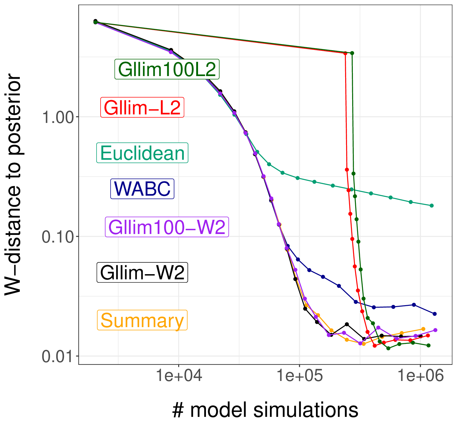
Note that this normal location model is exactly the GLLiM model for $K = 1$ and is therefore particularly favorable example. In such a simple case, computing BIC to select the number of GLLiM components, for values $K \geq 1$ shows a clear minimum at $K = 1$ . Using the GLLiM-iid formulas of Section S1.2.1 for $K = 1$ leads to closed form expressions for all parameter estimated and a Gaussian GLLiM posterior can be deduced with mean and covariance matrix of the above form. For $K = 1$ , the number of GLLiM parameters to estimate is very low (14) so that the number of simulated observations in the learning set can be small. We tested two GLLiM models learned with respectively $N = 10^{5}$ and $N = 100$ . When assessing the quality of the model parameters estimates, the larger $N$ the better but with $N = 100$ the approximation is already informative enough so that the GLLiM-ABC results remain good. This is illustrated in Figure S1 (c).

We compare GLLiM-ABC with three other methods: ABC using the Euclidean distance between the data sets, and ABC using the Euclidean distance between sample means, which for this model are sufficient summary statistics. All ABC posteriors are approximated by using the SMC sampler described in Section 2.1 of Bernton et al. (2019). To carry out the SMC-ABC procedure, we used the winference package from Bernton et al. (2019) and available at https://github.com/pierrejacob/winference. The code was adapted to incorporate MW₂ and L₂ distances, which in the $K = 1$ are closed form and simplify greatly. Let us denote

Δ (\hat{𝐲}, \hat{𝐳}) = \hat{𝚺}^{*} \tilde{𝑨}^{T} \tilde{𝚺}^{- 1} (\sum_{r = 1}^{R} 𝐲^{r} - \sum_{r = 1}^{R} 𝐳^{r}) .

The MW₂ distance reduces to the 2-Wasserstein distance between two Gaussian distributions with the same covariance matrices and leads to

M W_{2} (p_{G} (𝜽 | \hat{𝐲}), p_{G} (𝜽 | \hat{𝐳})) = | | Δ (\hat{𝐲}, \hat{𝐳}) | |_{2}^{2}

while for the L₂ distance we get,

L_{2}^{2} (p_{G} (𝜽 | \hat{𝐲}), p_{G} (𝜽 | \hat{𝐳})) = \frac{2}{\sqrt{2 π} | 2 \hat{𝚺}^{*} |^{1 / 2}} (1 - \exp (- \frac{1}{4} Δ (\hat{𝐲}, \hat{𝐳})^{T} \hat{𝚺}^{- 1} Δ (\hat{𝐲}, \hat{𝐳}))) .

Note that L₂ distance between empirical means is $| | \sum_{r = 1}^{R} 𝐲^{r} - \sum_{r = 1}^{R} 𝐳^{r} | |_{2}^{2}$ . In contrast, the Wasserstein distance between samples used in WABC does not reduce to a comparison of empirical means. As expected in this very particular case, it is less efficient both in terms of simulations and computing time.

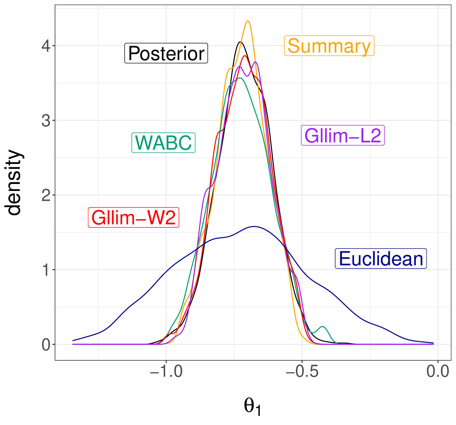
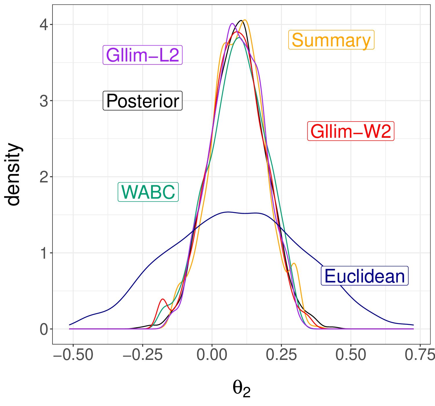
More specifically, all methods are run for a budget of $10^{6}$ model simulations, using $2048$ particles in the SMC sampler. Approximations of the marginal posterior distributions of the parameters are given in Figure S1 (a,b), illustrating that all SMC-based ABC methods except the one based on Euclidean distances between samples approximate the posterior accurately. The proximity of the obtained ABC samples and the posterior is quantified using also the Wasserstein distance. We independently draw 2048 samples from the posterior distribution and compute the Wasserstein distance between these samples and the 2048 ABC samples produced by the SMC algorithm. We plot the resulting distances against the number of model simulations in Figure S1 (c), on a log-log-scale. ABC with sufficient statistics converges fastest to the posterior and provides a reference behavior. The proposed GLLiM-ABC approach performs very similarly for MW₂ and when the number of simulations becomes large for L₂. The L₂ curve difference at the start is due to a requirement of the SMC implementation. A desired property is that the proportion of unique particles within the sample at each step is at least equal to a quantity $α$ , set to 0.5 by default. For some reason, in the L₂ case, the number of simulations required to meet this proportion is very high in the first step. Overall, WABC requires more model simulations to yield comparable results. In terms of computing time, WABC is much more costly due to the fact that MW₂ and L₂ are very simple in this case. The overall time to run the whole procedure was respectively of 1 min 30 s (GLLiM-MW₂-ABC), 2 min 32 s (GLLiM-L₂-ABC), 2 min 48 s (Euclidean ABC), 1 min 29 s (Summary stat. ABC) and 50 min (WABC).

As Bernton et al. (2019), we observe that SMC-ABC was much more efficient than simple rejection ABC. We therefore only show here results with GLLiM-SMC-ABC.

Refer to caption — Figure S1: Bivariate normal location model: (a) and (b) marginal posteriors for parameters $θ_{1}, θ_{2}$ with a SMC-ABC procedure, (c) Wasserstein distances between ABC samples and a posterior sample with respect to the number of simulations up to $M = 10^{6}$ . Gllim-L2 and GLLim-W2 (resp. Gllim100-L2 and GLLim100-W2) correspond to a GLLiM model learned with $N = 10^{5}$ (resp. $N = 100$ ) samples. Realisations are made of $R = 100$ i.i.d. observations.

S4 .2 Bivariate Beta model

The bivariate beta model proposed by Crackel and Flegal (2017) is defined with five positive parameters $θ_{1}, \dots, θ_{5}$ by letting

v_{1} = \frac{u_{1} + u_{3}}{u_{5} + u_{4}}, and v_{2} = \frac{u_{2} + u_{4}}{u_{5} + u_{3}},

(42)

where $u_{i} \sim Gamma (θ_{i}, 1)$ , for $i \in [5]$ , and setting $z_{1} = v_{1} / (1 + v_{1})$ and $z_{2} = v_{2} / (1 + v_{2})$ . The bivariate random variable $𝐳^{⊤} = (z_{1}, z_{2})$ has marginal laws $z_{1} \sim B e t a (θ_{1} + θ_{3}, θ_{5} + θ_{4})$ and $z_{2} \sim B e t a (θ_{2} + θ_{4}, θ_{5} + θ_{3})$ . We perform ABC using samples of size $R = 100$ . The observed sample is generated from the model with true parameter values $(θ_{1}, θ_{2}, θ_{3}, θ_{4}, θ_{5}) = (1, 1, 1, 1, 1)$ . The prior on each of the model parameters is taken to be independent and uniform over interval $[0, 5]$ .

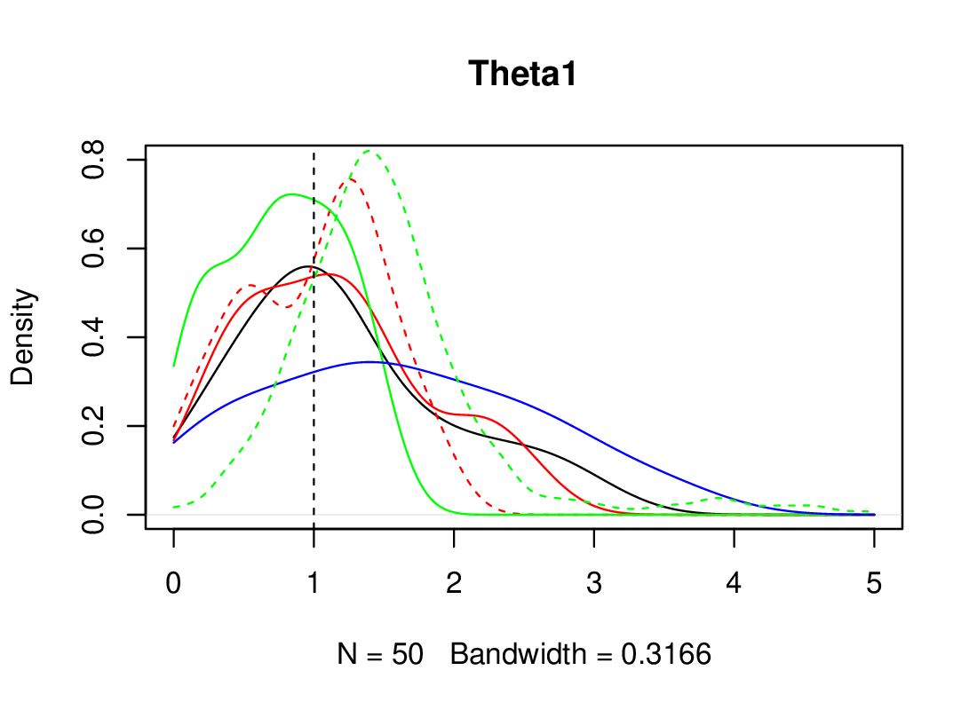
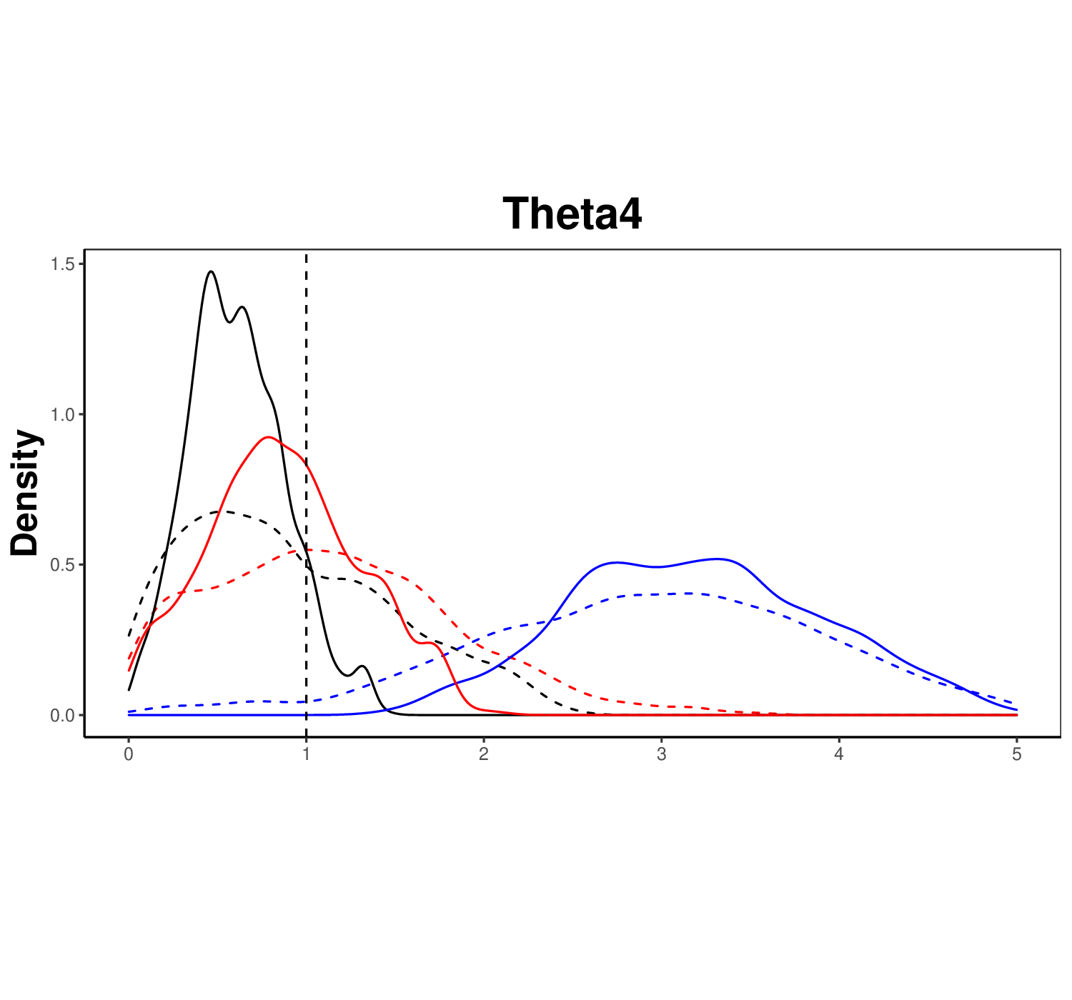
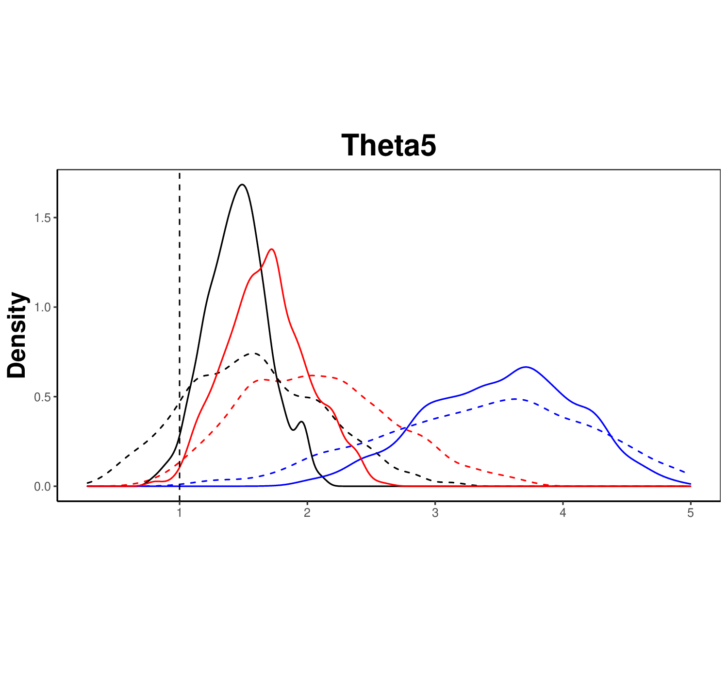
Figure S2 shows the marginal ABC posterior distributions for each of the 5 parameters and comparing 5 ABC procedures.

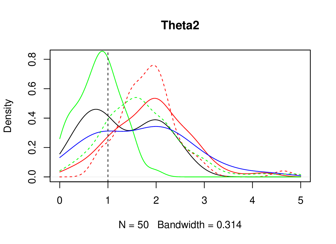
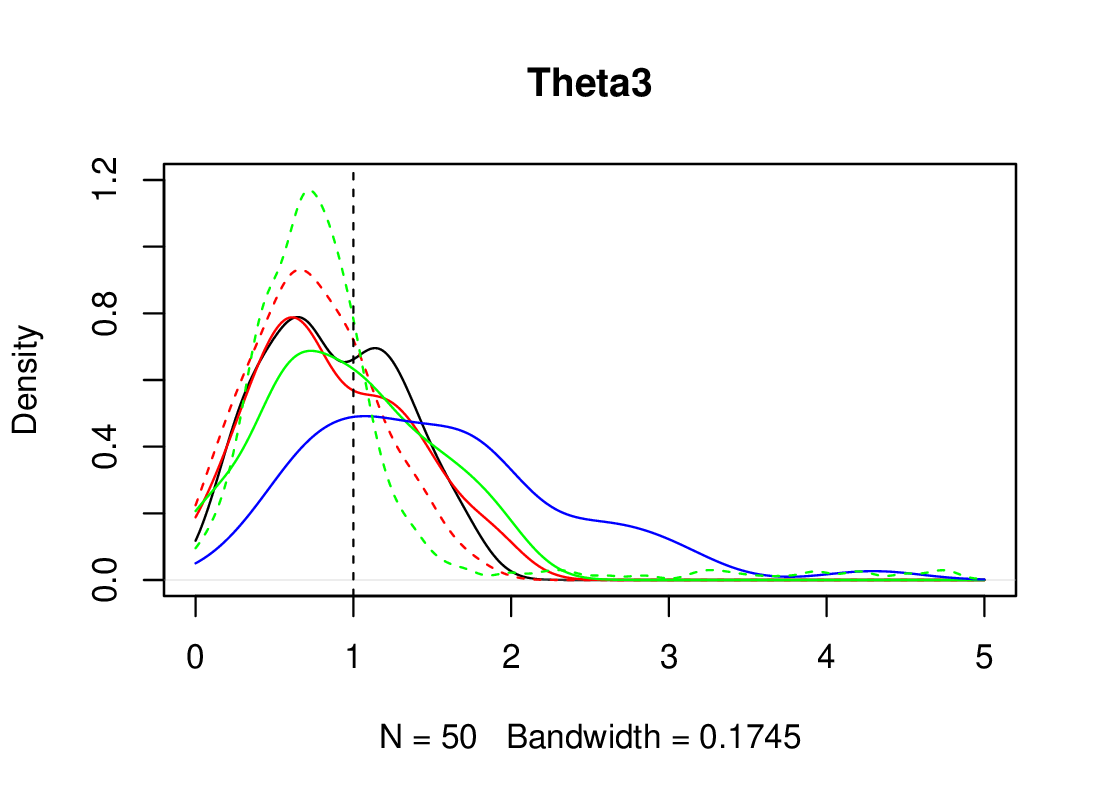
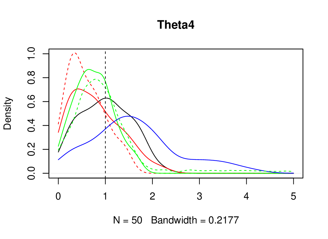
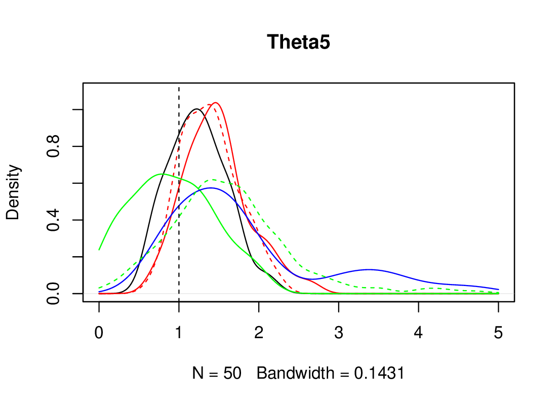
We then summarise each sample using 14 quantiles and apply the ABC procedures on these summarised data sets. The marginal posteriors are shown in Figure S3 for the 5 parameters and the 5 procedures. The GLLiM-MW2-ABC procedure based on the MW₂ distance is the best while the one based on L₂ performs very poorly. This is surprising as both methods are based on the same GLLiM surrogates. Understanding the failure of the L₂ distance in this specific case would require more investigations. The GLLiM mixture for the observation to be inverted is also shown and exhibits modes near the true parameters values. GLLiM-MW2-ABC and GLLiM-E-ABC perform similarly while the addition of log-variances in GLLiM-EV-ABC does not seem to improve posterior estimation. GLLiM-E-ABC and the semi-automatic method both rely on an estimation of the posterior means but show posteriors of different shapes in particular for $θ_{1}$ and $θ_{4}$ (Figure S3). Differences between the two methods are also observed in Figure S2 for $θ_{2}$ and $θ_{4}$ but in this case the two methods do not used the same summaries.

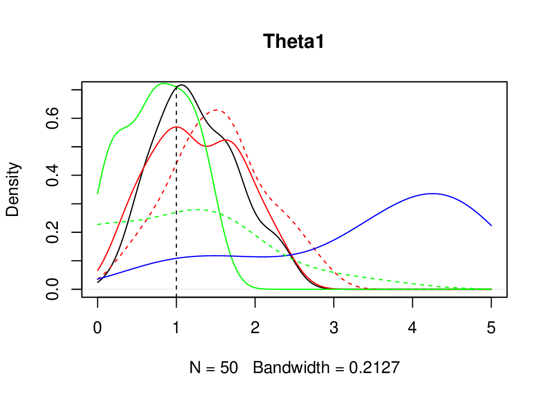
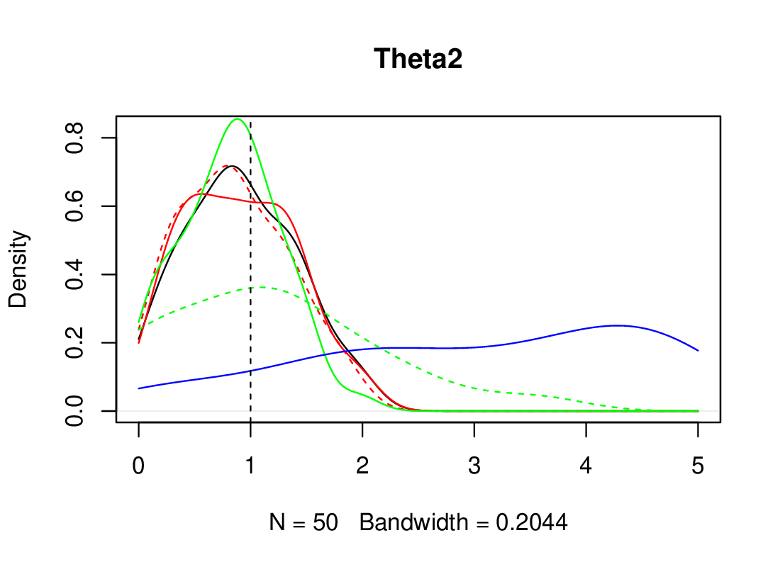
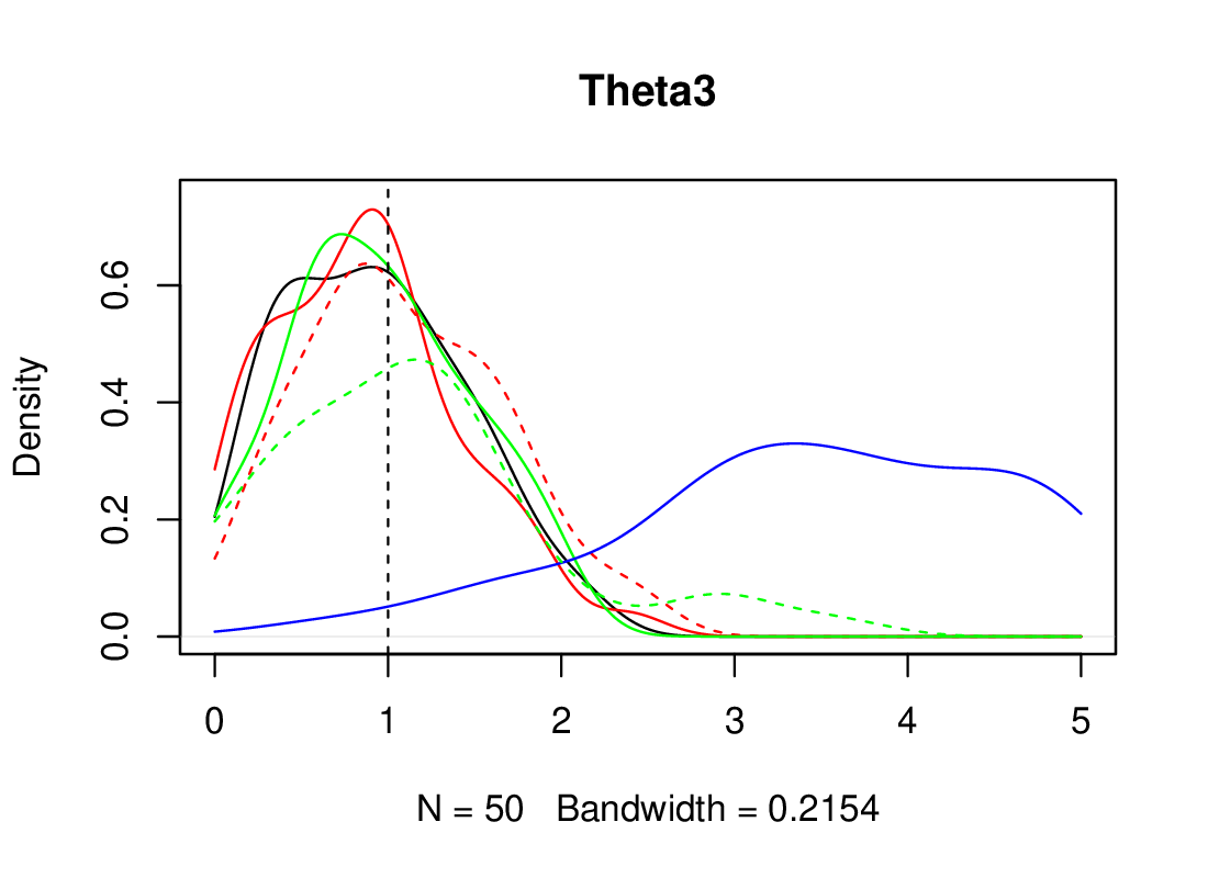
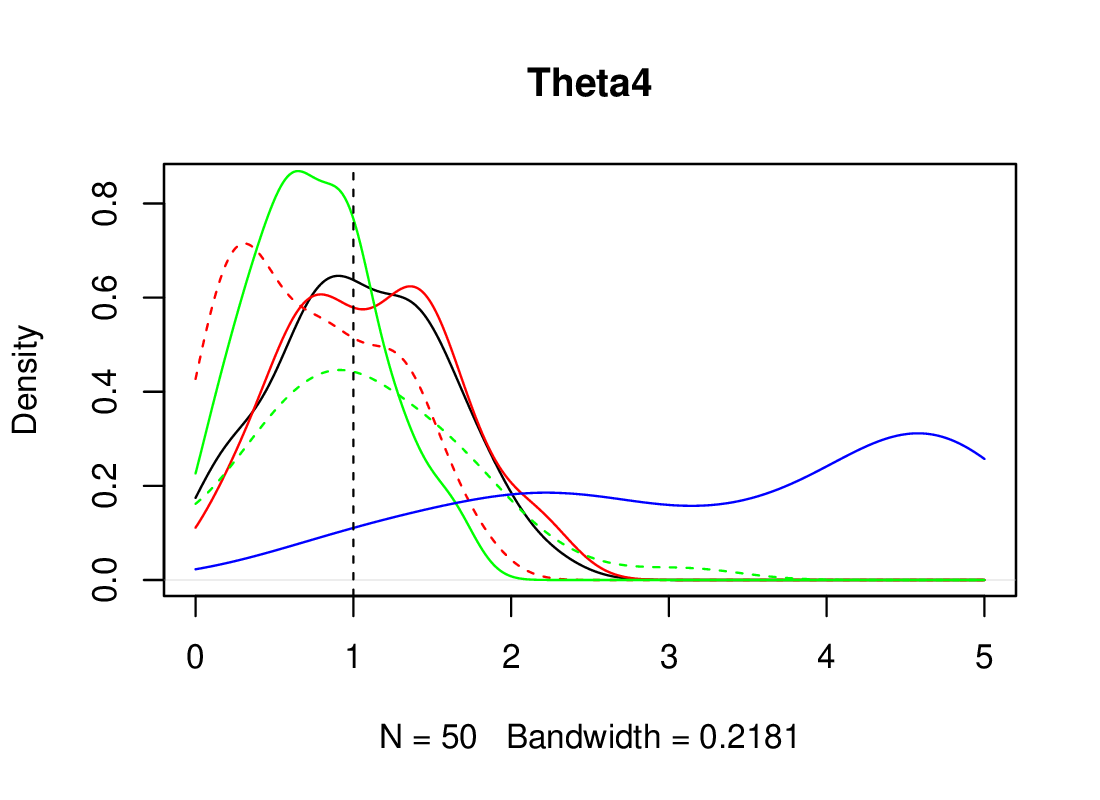
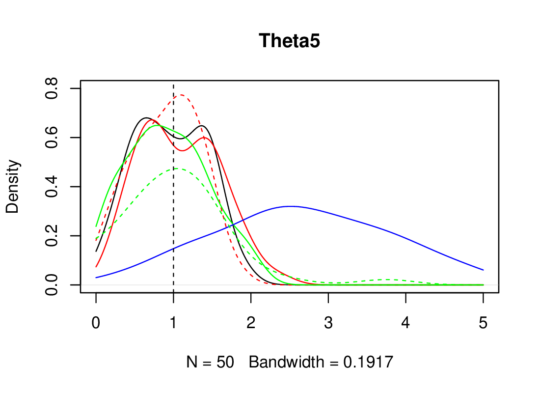
For a more quantitative comparison, we compute for each posterior samples of size $S$ , empirical means of the parameters, $\bar{θ}_{j} = \frac{1}{S} \sum_{i = 1}^{S} θ_{j}^{i}$ , and empirical root mean square errors (RMSE) defined as $R (θ_{j}) = \sqrt{\frac{1}{S} \sum_{i = 1}^{S} (θ_{j}^{i} - θ_{j}^{0})^{2}}$ where $j \in [5]$ , $S = 50$ and $θ_{j}^{i}$ is the sample $i$ for $θ_{j}$ and $θ_{j}^{0}$ is the true parameter value. Table S1 shows these quantities for the posteriors shown in Figures S2 and S3.

Rejection ABC
Procedure	$\bar{θ}_{1}$	$\bar{θ}_{2}$	$\bar{θ}_{3}$	$\bar{θ}_{4}$	$\bar{θ}_{5}$	R( $θ_{1}$ )	R( $θ_{2}$ )	R( $θ_{3}$ )	R( $θ_{4}$ )	R( $θ_{5}$ )
GLLiM mixture	1.504	1.736	0.890	0.989	1.616	0.926	1.276	0.824	0.848	1.021
GLLiM-E-ABC	1.142	1.899	0.871	0.786	1.472	0.678	1.181	0.498	0.568	0.626
GLLiM-EV-ABC	0.990	1.867	0.746	0.594	1.385	0.505	1.077	0.469	0.562	0.517
GLLiM-L2-ABC	1.597	1.700	1.534	1.627	1.827	1.1445	1.224	0.968	1.117	1.295
GLLiM-MW2-ABC	1.211	1.319	0.872	1.004	1.235	0.790	0.820	0.439	0.523	0.426
	with 14 quantiles as summaries
Semi-auto ABC	0.770	0.825	0.947	0.756	0.917	0.493	0.472	0.524	0.468	0.523
GLLiM mixture	0.448	0.858	0.739	0.552	0.577	1.685	1.464	1.367	1.300	1.214
GLLiM-E-ABC	1.266	0.905	0.872	1.105	1.082	0.629	0.501	0.550	0.541	0.514
GLLiM-EV-ABC	1.530	0.852	1.095	0.727	0.904	0.808	0.504	0.577	0.565	0.450
GLLiM-L2-ABC	3.390	3.010	3.467	3.361	2.653	2.747	2.492	2.693	2.732	1.995
GLLiM-MW2-ABC	1.257	0.909	0.921	1.042	0.950	0.573	0.500	0.524	0.529	0.464
SMC-ABC
GLLiM-L2 ( $10^{5}$ )	2.133	2.581	2.443	2.345	3.074	1.394	1.985	1.996	1.735	2.217
GLLiM-L2 ( $10^{6}$ )	1.875	2.948	3.715	3.062	3.430	1.438	2.280	2.908	2.147	2.513
GLLiM-MW2 ( $10^{5}$ )	1.149	1.849	0.641	0.524	1.417	0.575	1.071	0.563	0.558	0.502
GLLiM-MW2 ( $10^{6}$ )	1.316	1.656	0.684	0.708	1.495	0.508	0.852	0.399	0.421	0.547
WABC ( $10^{5}$ )	1.871	1.790	0.755	0.939	1.767	1.158	1.201	0.502	0.508	0.818
WABC ( $10^{6}$ )	1.546	1.732	0.769	0.821	1.566	0.773	0.880	0.373	0.365	0.621

Table S1: Bivariate Beta model: parameter means, and RMSE (

R (\cdot)

) for ABC posterior distributions shown in Figures S2, S3 and S4 when the observed data is generated with

𝜽 = (1, 1, 1, 1, 1)

. The ABC posterior values are computed as empirical values over samples of size 50. SMC-ABC uses different simulated samples. Two simulation budgets are compared with

M = 10^{5}

and

M = 10^{6}

simulations respectively. Means closest to 1 and best (lowest) RMSE values are in boldface.

S4 .2.1 SMC-ABC and WABC

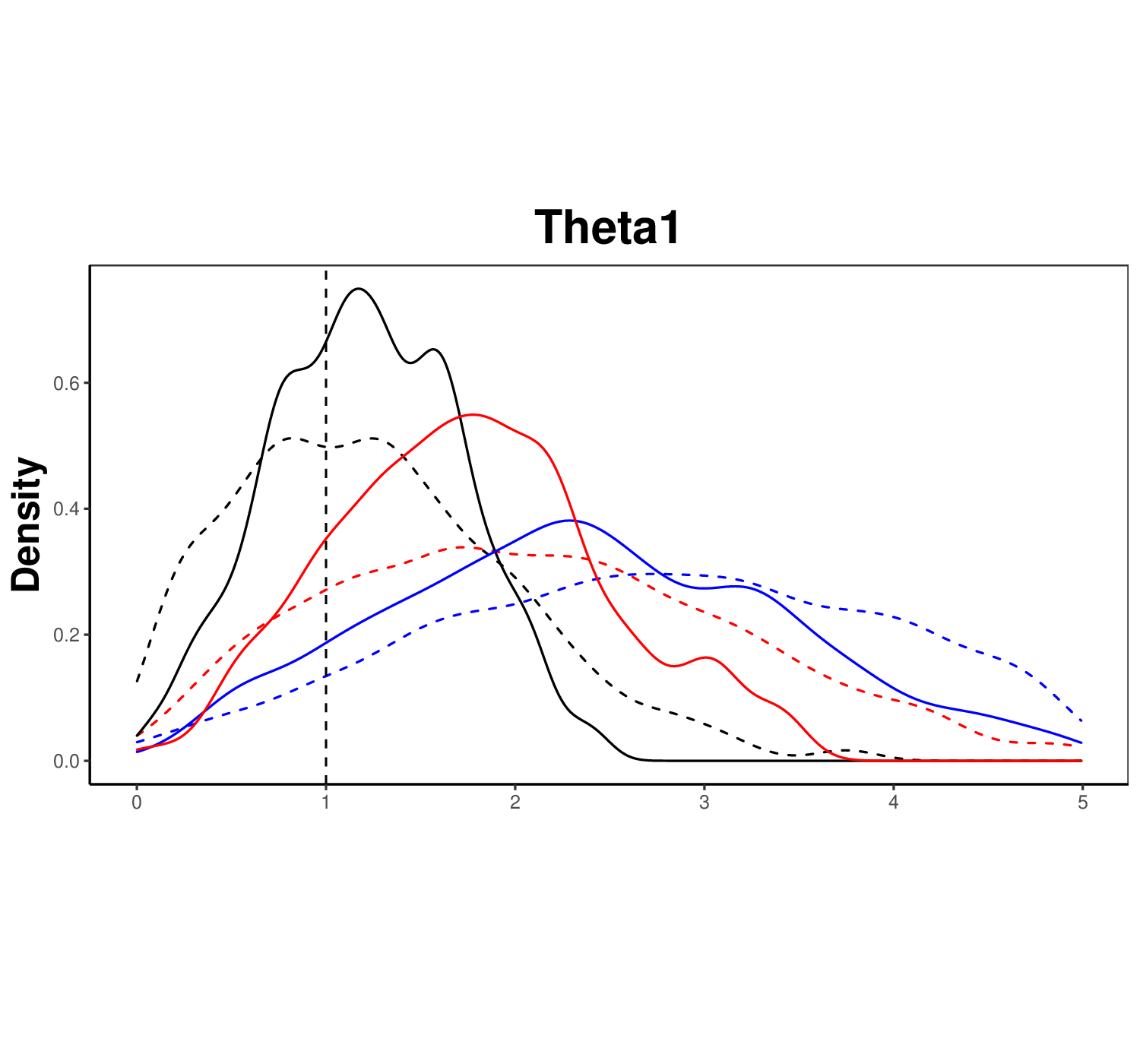
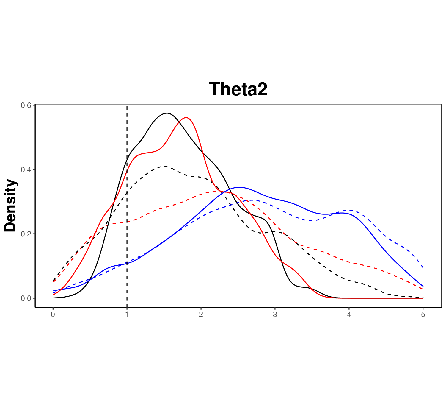
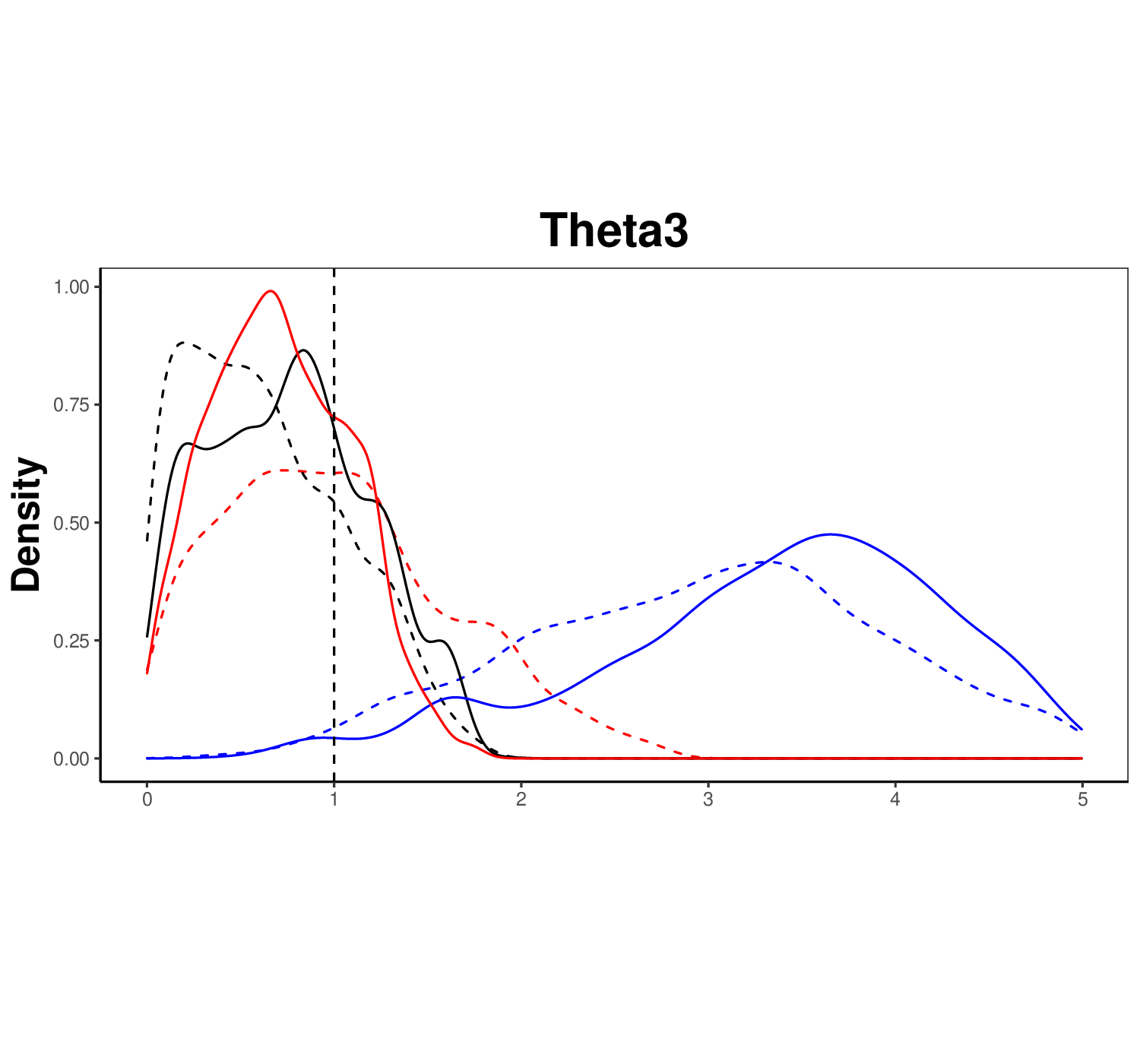
We then compared the MW₂ and L₂ variants of GLLiM to WABC of Bernton et al. (2019). To do this, we consider SMC-ABC instead of rejection ABC. The SMC-ABC procedure follows that of Bernton et al. (2019). The number of particles is set to 2048 and a budget of $M = 10^{5}$ and $M = 10^{6}$ is considered successively. Table S1 and Figure S4 show the resulting posterior approximations. Except for the L₂ distance, it illustrates the concentration of the posterior distributions when the number of simulations increases.

S4 .3 Moving average model

The MA(2) process is a stochastic process $(y^{'}_{t})_{t \in ℕ^{*}}$ defined by

y^{'}_{t} = z_{t} + θ_{1} z_{t - 1} + θ_{2} z_{t - 2},

(43)

where ${z_{t}}$ is an i.i.d. sequence, according to a standard normal distribution and $θ_{1}$ and $θ_{2}$ are scalar parameters. A standard identifiability condition is imposed on this model leading to a prior distribution on the triangle described by the inequalities

- 2 < θ_{1} < 2, θ_{1} + θ_{2} > - 1, θ_{1} - θ_{2} < 1 .

As in most papers, the prior on the two model parameters is taken uniform over the triangular domain. Natural summary statistics for this model are the empirical auto-covariances of lag 1 and 2, which converge to a one-to-one function of the two parameters. This example is a way to illustrate our method on time series in the same manner as Bernton et al. (2019). Their Wasserstein-ABC proposal uses empirical distributions and, like other data discrepancy based methods, is in principle only valid for i.i.d. observations. However, they also investigate the use of the method to time series where observations are not i.i.d.. We make a similar attempt in this work and show how it can be interpreted in our framework.

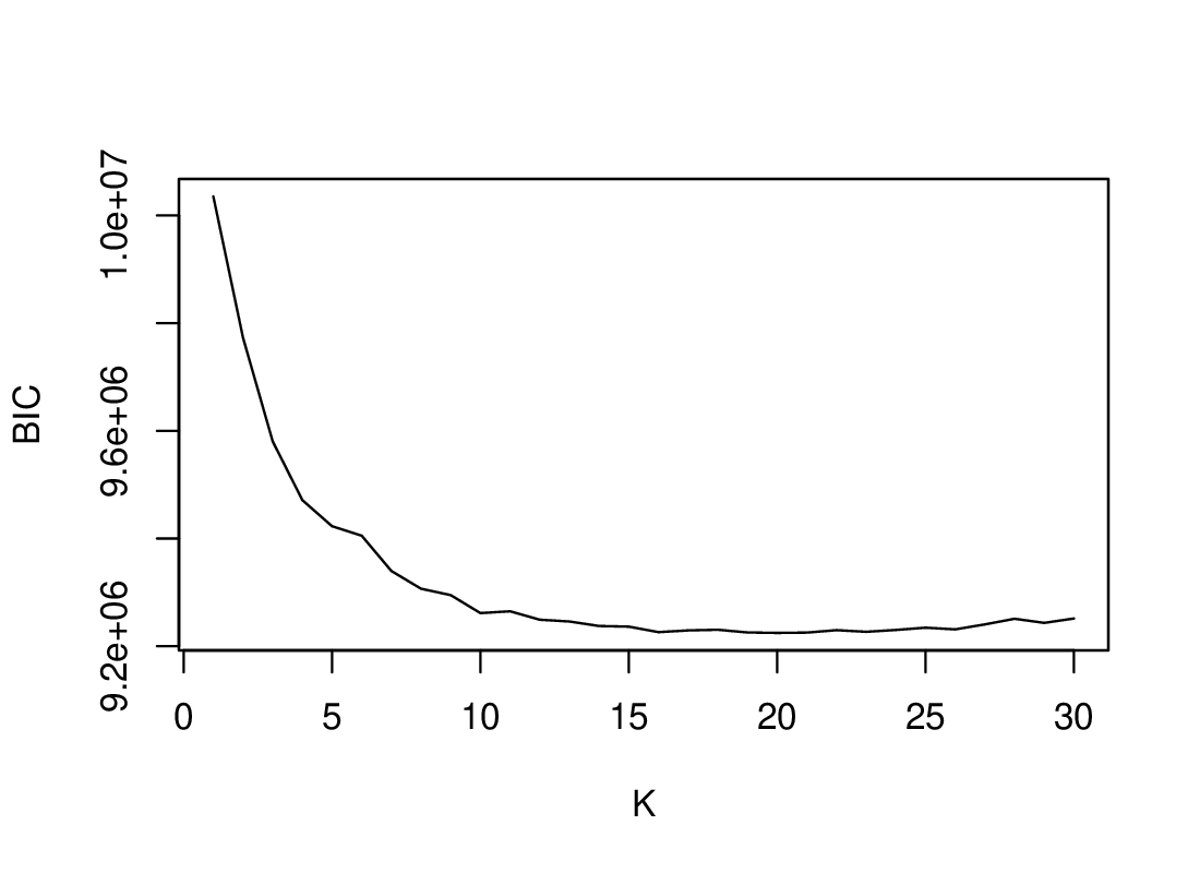
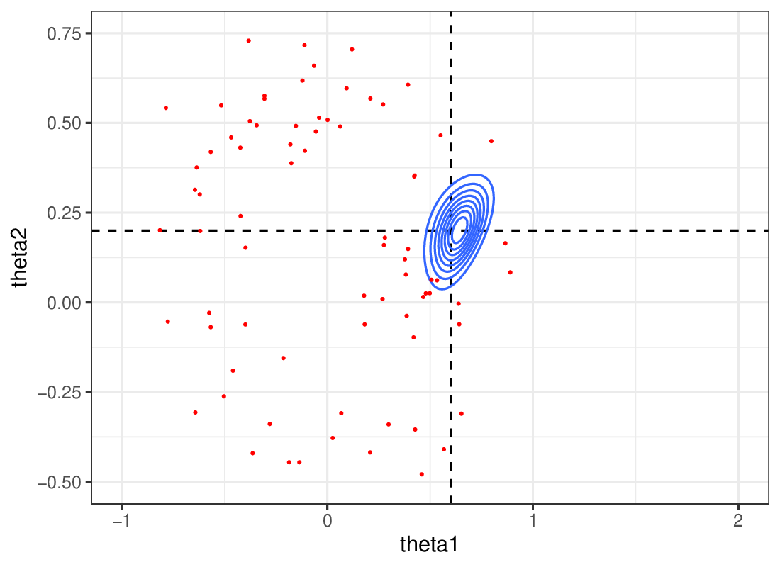
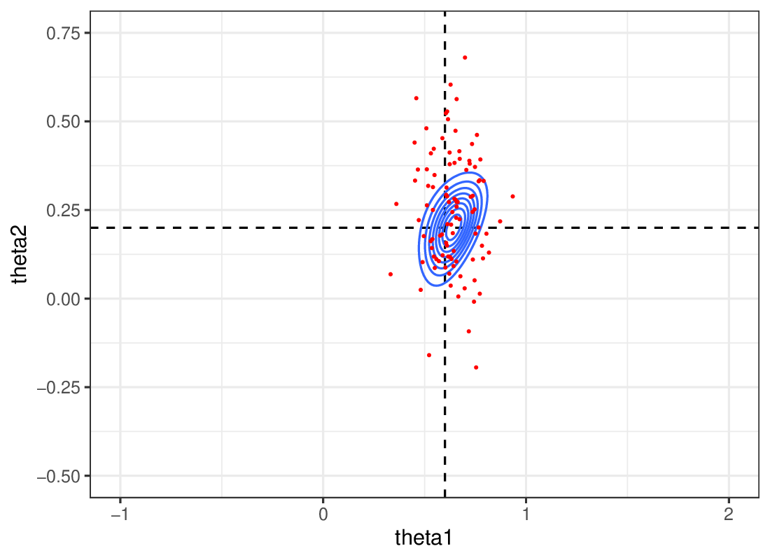
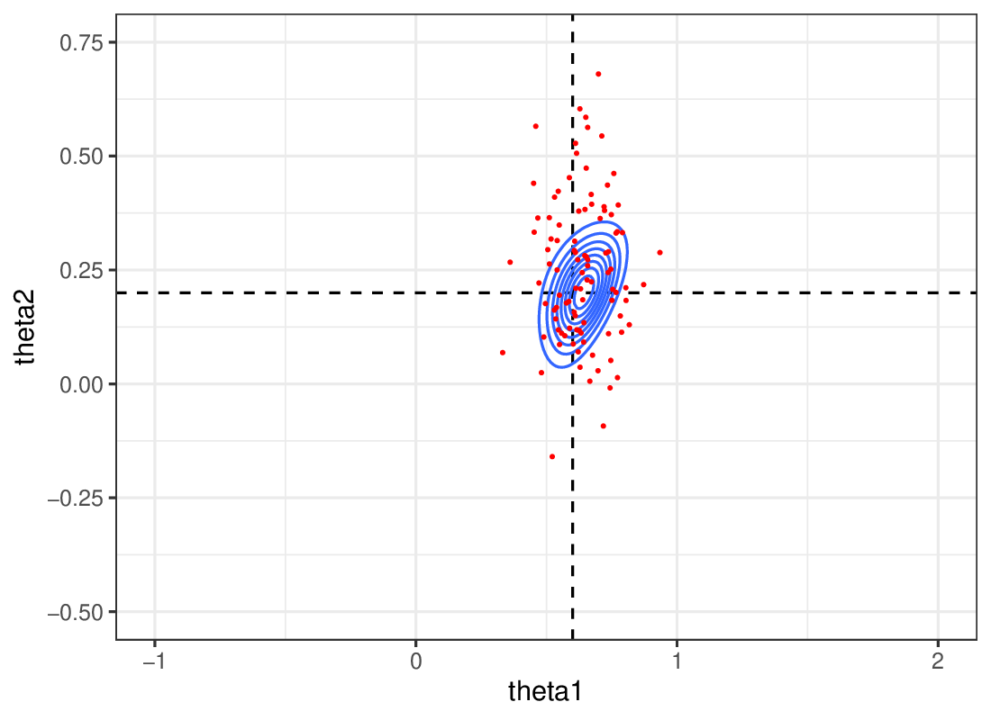
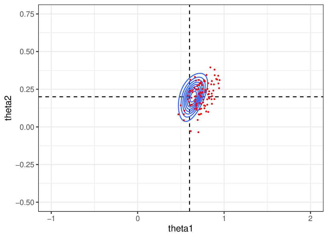
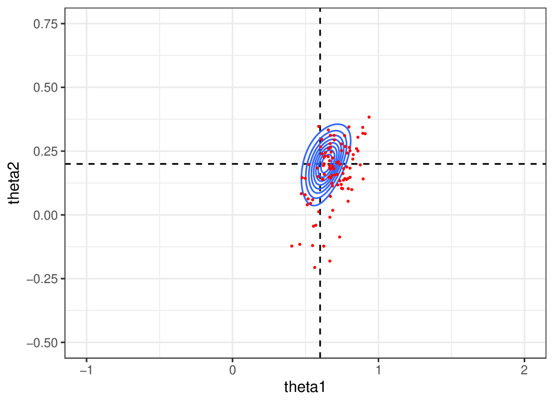
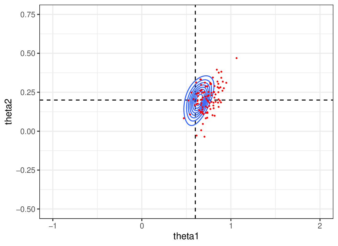
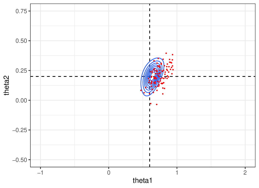
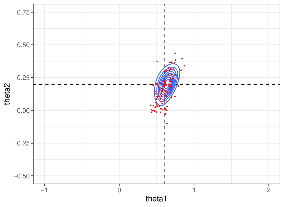
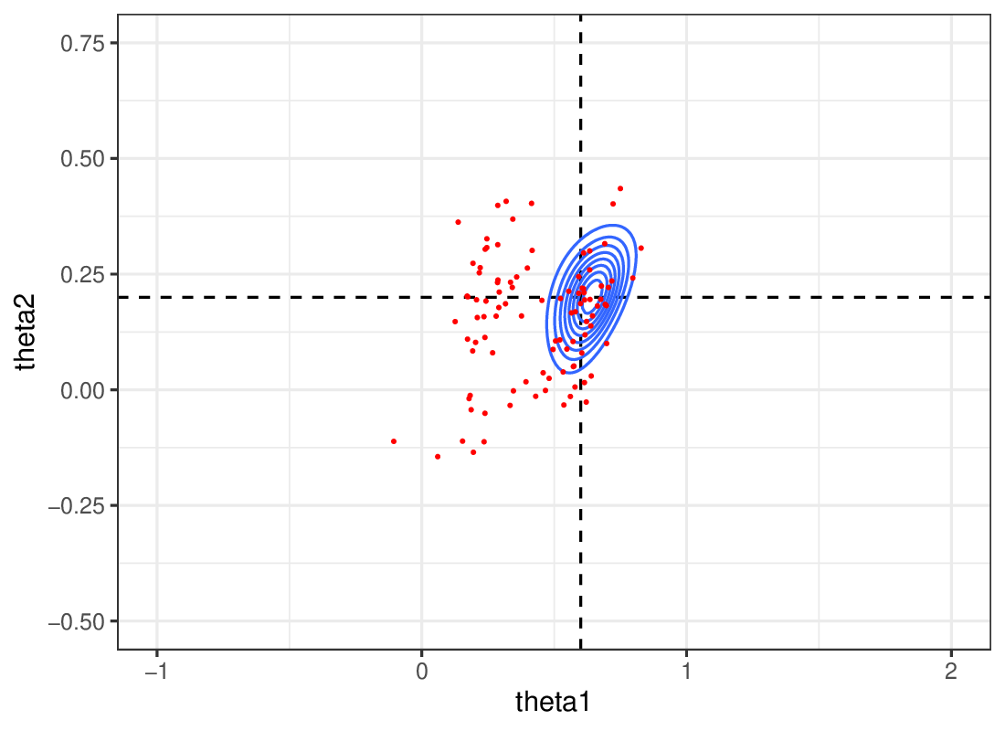
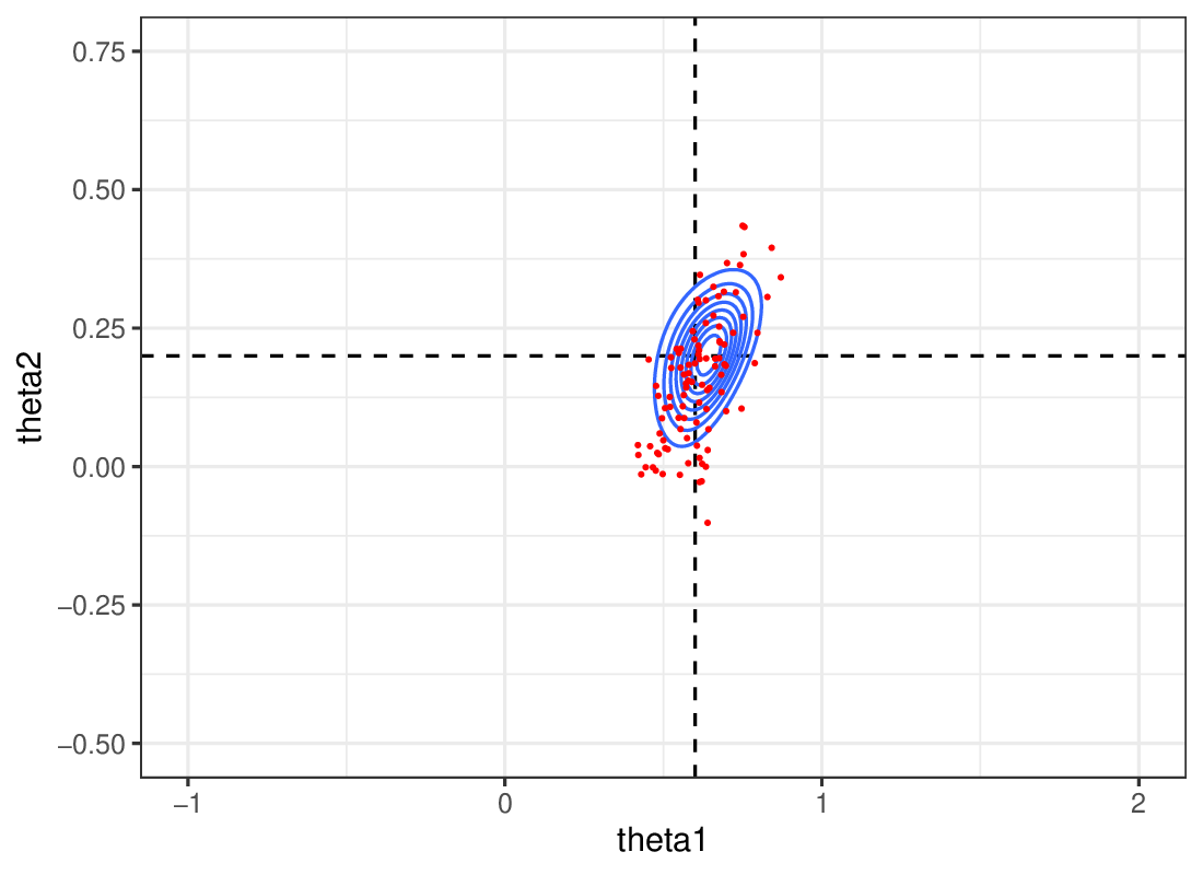
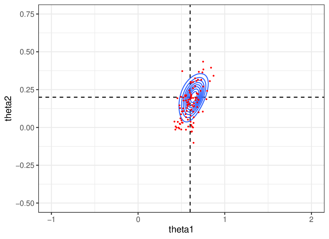
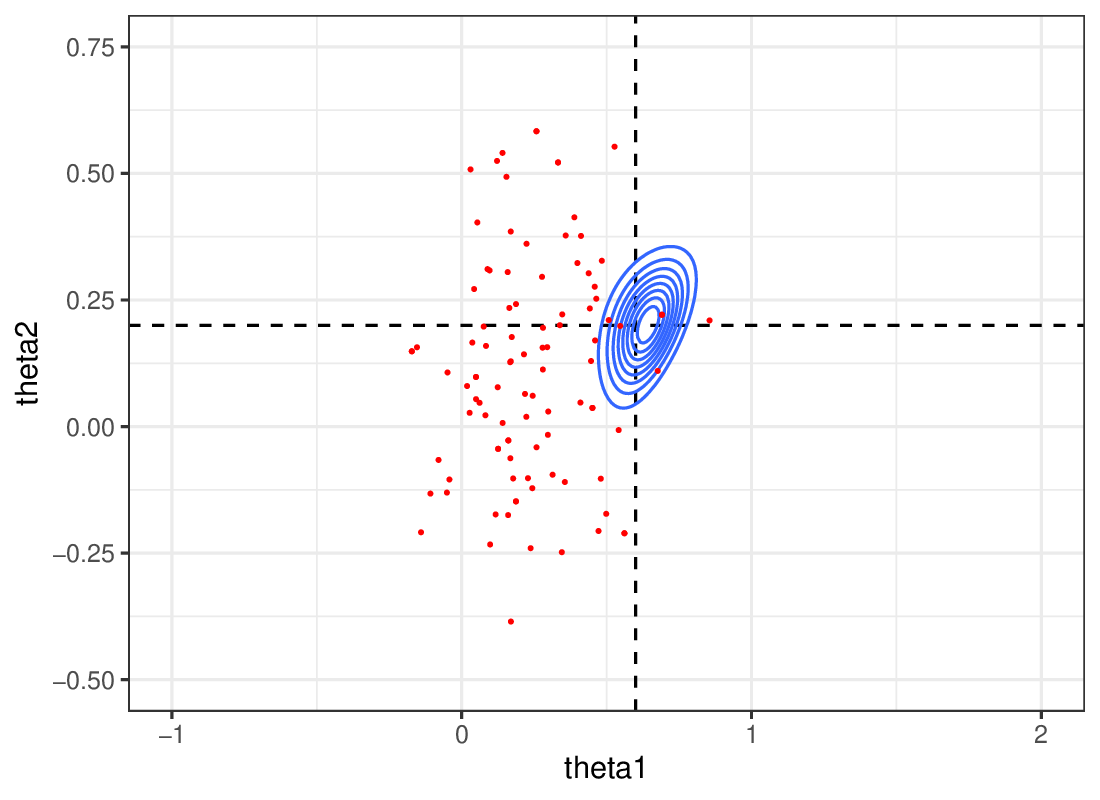
For each pair of parameters $(θ_{1}, θ_{2})$ in the triangular domain, a series of length 150 is simulated according to the MA(2) model (43). We consider time series of length 150, instead of 100 in Jiang et al. (2017). This is repeated $N$ times so that the number of pairs in the learning set is $N = 10^{5}$ . The series to be inverted is simulated similarly with true parameters $θ_{1} = 0.6$ and $θ_{2} = 0.2$ . To learn a GLLiM model with $d = 150$ , $ℓ = 2$ , $K = 30$ , and no constraints on the covariance matrices for the likelihood part of the model, requires the estimation of 353429 parameters. To reduce the model complexity while going beyond the alternative isotropic or diagonal cases, we propose to use the i.i.d. adaptation of GLLiM. GLLiM is applied with $d = 3$ , $R = 50$ and no constraint on the $3 \times 3$ blocks themselves (629 parameters). A second experiment is made with $R = 5$ and $d = 30$ i.e. with 5 blocks of size $30 \times 30$ with no constraint on the block structure (16829 parameters) . The second setting is retained as it shows better precision on $θ_{2}$ in particular. In terms of approximation this is equivalent to neglect only few correlations in the GLLiM approximation of the likelihood. To illustrate the possibility to select $K$ , we compute the Bayesian Information Criterion (BIC) for $K = 2$ to 30. Figure S5 shows the resulting BIC values. A minimum is observed for $K = 20$ but values after $K = 15$ provide similar BIC values. The GLLiM-ABC results with $K = 20$ and $K = 30$ are different but of similar overall quality (see below).

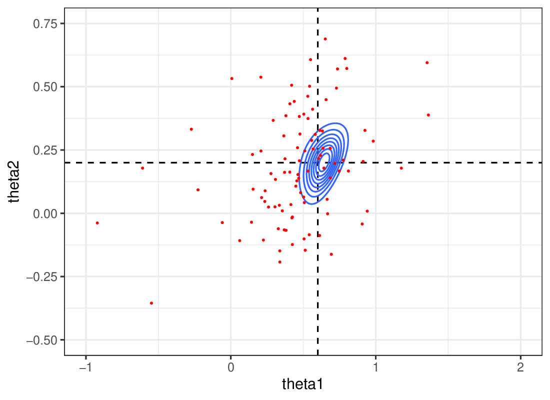
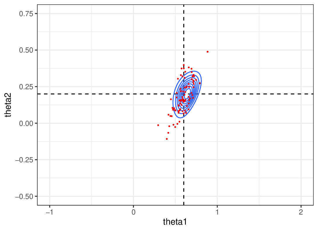
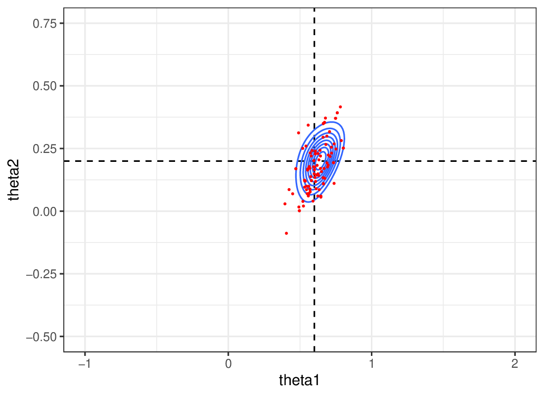
For rejection ABC procedures, the tolerance threshold $ϵ$ is set to the 0.1% quantile leading to selected samples of size 100. Empirical values for parameter means, standard deviations and correlation when applying the different ABC schemes for one observed time series are compared to the true ones computed numerically. The true posterior means, standard deviations of $θ_{1}$ and $θ_{2}$ are computed numerically using importance sampling. The true posterior correlation between $θ_{1}$ and $θ_{2}$ is also computed this way. The corresponding ABC estimations and samples are shown in Table S2 and Figure S6. The results are qualitatively similar to that of Jiang et al. (2017) with a poor estimation of the means for the semi-automatic ABC procedure on the full time series. They also confirm results already observed in previous works, namely that semi-automatic and auto-covariance-based procedures do not well capture correlation information between $θ_{1}$ and $θ_{2}$ . Surprisingly, the GLLiM mixture approximation of the posterior also provides a poor estimation of the correlation but this estimation improves a lot when adding the ABC step. Results with a SMC-ABC procedure are also shown in Table S2 and Figure S6. The results obtained with WABC are not satisfying but this is due to the low number of i.i.d. repetitions $R = 5$ for which the method based on histograms comparison is not efficient. For our MW₂ and L₂ implementations with a $K = 20$ component GLLiM, the results improve for all estimated quantities except for the correlation (see Table S2).

Table S2: MA(2) model: parameter means, standard deviations and correlations for the exact and ABC posterior distributions shown in Figure S6 when the observed data is generated with

θ_{1} = 0.6

and

θ_{2} = 0.2

. The exact posterior values are computed numerically, while the ABC posterior values are computed as empirical values over samples of size 100. Rejection ABC is used except when specified with using a SMC postfix. Closest values to the true posterior ones are in bold.

Posterior	mean( $θ_{1}$ )	mean( $θ_{2}$ )	std( $θ_{1}$ )	std( $θ_{2}$ )	cor( $θ_{1}, θ_{2}$ )
Exact	0.635	0.203	0.080	0.076	0.472
Auto-cov Rejection ABC	0.635	0.246	0.107	0.164	0.018
Auto-cov Semi-auto	0.637	0.250	0.109	0.159	-0.045
Semi-auto ABC	0.026	0.027	0.406	0.476	-0.112
WABC	0.242	0.117	0.204	0.218	0.109
$K = 30$
GLLiM mixture	0.521	0.182	0.499	0.294	-0.007
GLLiM-E-ABC	0.737	0.208	0.104	0.084	0.454
GLLiM-EV-ABC	0.689	0.163	0.110	0.120	0.474
GLLiM-L2-ABC	0.740	0.213	0.103	0.088	0.436
GLLiM-MW2-ABC	0.742	0.206	0.104	0.084	0.527
$K = 20$
GLLiM mixture	0.430	0.209	0.415	0.241	0.055
GLLiM-E-ABC	0.608	0.157	0.097	0.117	0.609
GLLiM-EV-ABC	0.435	0.156	0.201	0.131	0.217
GLLiM-L2-ABC	0.608	0.158	0.096	0.117	0.632
GLLiM-MW2-ABC	0.605	0.155	0.096	0.113	0.581
GLLiM-L2-SMC	0.617	0.194	0.113	0.120	0.727
GLLiM-MW2-SMC	0.618	0.176	0.088	0.102	0.605

S4 .4 Non-identifiable models

Our main targets are posterior distributions with multiple modes for which our method is more likely to provide significantly better performance than existing approaches. It is straightforward to construct models that lead to multimodal posteriors by considering likelihoods that are invariant by some transformation.

S4 .4.1 Ill-posed inverse problems

Here, we consider inverse problems for which the solution is not unique. This setting is quite common in practice and can occur easily when the forward model exhibits some invariance, e.g., when considering the negative of the parameters. A simple way to model this situation consists of assuming that the observation $𝐲$ is generated as a realization of

𝐲

= F (𝜽) + 𝜺,

where $F$ is a deterministic theoretical model coming from experts and $𝜺$ is a random variable expressing the uncertainty both on the theoretical model and on the measurement process. A common assumption is that $𝜺$ is distributed as a centered Gaussian noise. Non-identifiability may then arise when $F (- 𝜽) = F (𝜽)$ . Following this generative approach, a first simple example is constructed with a Student $t$ -distributed noise leading to the likelihood:

f_{𝜽} (𝐲)

= 𝒮_{d} (𝐲; μ^{2} 1I_{d}, σ^{2} I_{d}, ν),

where $𝒮_{d} (\cdot; μ^{2} 1I_{d}, σ^{2} I_{d}, ν)$ is the pdf of a $d$ -variate Student $t$ -distribution with a $d$ -dimensional location parameter with all dimensions equal to $μ^{2}$ , diagonal isotropic scale matrix $σ^{2} I_{d}$ and degree-of-freedom (dof) parameter $ν$ . Recall that for a Student $t$ -distribution, a diagonal scale matrix is not inducing independent dimensions so that $𝐲$ is not a set of i.i.d. univariate Student $t$ observations. The dof controls the tail heaviness; i.e., the smaller the value of $ν$ , the heavier the tail. In particular, for $ν \leq 2$ , the variance is undefined, while for $ν \leq 1$ the expectation is also undefined. In this example, we set $σ^{2} = 2$ , $ν = 2.1$ , and $μ$ is the parameter to estimate.

For all compared procedures, we set $d = 10$ , $K = 10$ , $N = M = 10^{5}$ , and the tolerance level $ϵ$ to the $0.1 %$ quantile of observed distances, so that all selected posterior samples are of size 100.

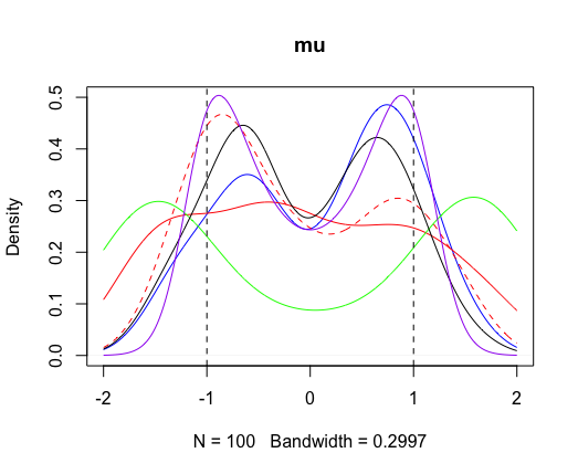
Figure S7 shows the true and the compared ABC posterior distributions for a 10-dimensional observation $𝐲$ , simulated under a process with $μ = 1$ . The true posterior exhibits the expected symmetry with modes close to the values: $μ = 1$ and $μ = - 1$ . The simple rejection ABC procedure based on GLLiM expectations (GLLiM-E-ABC) and the semi-automatic ABC procedure both show over dispersed samples with wrongly located modes. The GLLiM-EV-ABC exhibits two well located modes but does not preserve the symmetry of the true posterior. The distance-based approaches, GLLiM-L2-ABC and GLLiM-MW2-ABC both capture the bimodality. GLLiM-MW2-ABC is the only method to estimate a symmetric posterior distribution with two modes of equal importance. Note, however, that in term of precision, the posterior distribution estimation remains difficult considering an observation of size only $d = 10$ .

This simple example shows that the expectation as a summary statistic suffers from the presence of two equivalent modes, while the approaches based on distances are more robust. There is a clear improvement in complementing the summary statistics with the log-variances. Although in this case, this augmentation provides a satisfying bimodal posterior estimate, it lacks the expected symmetry of the two modes. The GLLiM-MW2-ABC procedure has the advantage of exhibiting a symmetric posterior estimate, that is more consistent with the true posterior.

In the following subsection we present another case that cannot be cast as the above generating process but also exhibit a transformation invariant likelihood.

S4 .4.2 Sum of moving average models of order 2 (MA(2))

Using the same MA(2) process as already defined in Section S4 .3, we consider a transformation that consists of taking the opposite sign of $θ_{1}$ and keeping $θ_{2}$ unchanged. The considered observation corresponds then to a series obtained by summing the two MA models, defined below

y^{'}_{t} = z_{t} + θ_{1} z_{t - 1} + θ_{2} z_{t - 2}, y^{''}_{t} = z^{'}_{t} - θ_{1} z^{'}_{t - 1} + θ_{2} z^{'}_{t - 2}, y_{t} = y^{'}_{t} + y^{''}_{t},

where ${z_{t}}$ and ${z^{'}_{t}}$ are both i.i.d. sequences, generated from a standard normal distribution. It follows that a vector of length $d$ , $𝐲 = (y_{1}, \dots, y_{d})^{⊤}$ , is distributed according to a multivariate $d$ -dimensional centered Gaussian distribution with a Toeplitz covariance matrix whose first row is $(2 (θ_{1}^{2} + θ_{2}^{2} + 1), 0, 2 θ_{2}, 0, \dots, 0)$ . The likelihood is therefore invariant by the transformation proposed above, and so is the uniform prior over the triangle. It follows that the posterior is also invariant by the same transformation and can then be chosen so as to exhibit two symmetric modes.

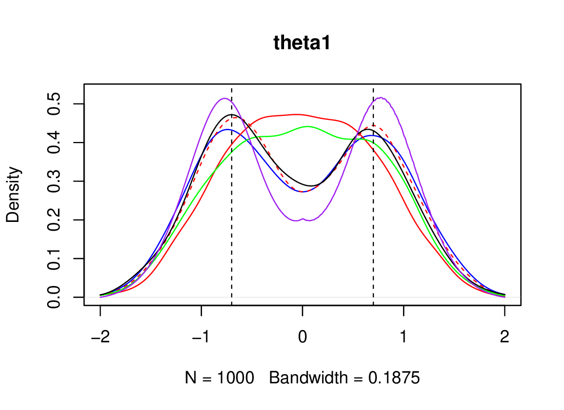
For all procedures, we set $K = 80$ and $N = M = 10^{5}$ , and $ϵ$ to the $1 %$ distance quantile, so that all selected posterior samples are of size 1000. An observation of size $d = 10$ is simulated from the model with $θ_{1} = 0.7$ and $θ_{2} = 0.5$ . ABC posterior distribution estimates are shown in Figure S8.

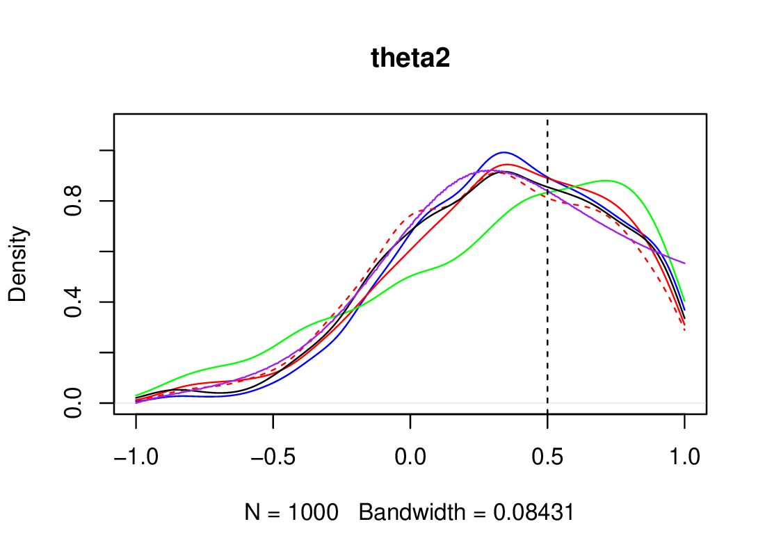The level sets of the true posterior can be computed from the exact likelihood and a grid of values for $θ_{1}$ and $θ_{2}$ . For the setting used here, none of the considered ABC procedures is fully satisfactory, in that the selected samples are all quite dispersed. This is mainly due to the relatively low size of the observation ( $d = 10$ ). The tests made in Section S4 .3 with a much larger $d = 150$ provided in contrast very satisfying samples as visible in supplementary Figure S3. This can also be observed in Marin et al. (2012) (Figures 1 and 2), where ABC samples are less dispersed for a size of $d = 100$ and quite spread off when $d$ is reduced to $d = 50$ , even when the autocovariance is used as summary statistic.

Despite the relative spread of the parameters accepted after the ABC rejection, the posterior marginals, shown in Figure S8, provide an interesting comparison. GLLiM-D-ABC and GLLiM-EV-ABC procedures show symmetric $θ_{1}$ values, in accordance with the symmetry and bimodality of the true posterior. The use of the L₂ or MW₂ distances does not lead to significant differences. GLLiM-E-ABC and semi-automatic ABC behave similarly and do not capture the bimodality on $θ_{1}$ , but the addition of the posterior log-variances in GLLiM-EV-ABC improves on GLLiM-E-ABC. These results suggest that although GLLiM may not provide good approximations of the first posterior moments, it can still provide good enough approximations of the surrogate posteriors in GLLiM-D-ABC. For $θ_{2}$ , all posteriors are rather close to the true posterior marginal except for semi-automatic ABC which shows a mode at a wrong location when compared to the true posterior.

A similar example using MA(1) processes is also provided in the next subsection.

S4 .4.3 Sum of moving average models of order 1 (MA(1))

The MA(1) process is a stochastic process $(y^{'}_{t})_{t \in ℕ^{*}}$ defined by

y^{'}_{t}

= z_{t} + ρ z_{t - 1} .

In order to construct bimodal posterior distributions, we consider the following sum of two such models. At each discrete time step $t$ we define,

y^{'}_{t} = z_{t} + ρ z_{t - 1}, y^{''}_{t} = z^{'}_{t} - ρ z^{'}_{t - 1}, and y_{t} = y^{'}_{t} + y^{''}_{t}

where ${z_{t}}$ and ${z^{'}_{t}}$ are both i.i.d. sequences, according to a standard normal distribution and $ρ$ is an unknown scalar parameter. It follows that a vector of length $d$ , $𝐲 = (y_{1}, \dots, y_{d})^{⊤}$ is distributed according to a multivariate $d$ -dimensional centered Gaussian distribution with an isotropic covariance matrix whose diagonal entries are all equal to $2 (ρ^{2} + 1)$ . The likelihood is therefore invariant by symmetry about 0 and so is the prior on $ρ$ assumed to be uniform over $[- 2, 2]$ . It follows that the posterior on $ρ$ is also invariant by this transformation and can thus be chosen so as to exhibit two symmetric modes. The true posterior looks similar to the one in Section S4 .4 but $ρ$ is now a parameter impacting upon the variance of the likelihood.

For all procedures, we set $N = M = 10^{5}$ , and $ϵ$ to the $0.1 %$ quantile of observed distances so that all selected posterior samples are of size 100. In terms of difficulty, the main difference with the example in Section S4 .4 lies in a higher non-linearity of the likelihood and of the model joint distribution. We then report results with a higher choice of $K = 20$ . When $K = 10$ , results are similar except for GLLiM-EV-ABC, which does not show improvement over GLLiM-E-ABC.

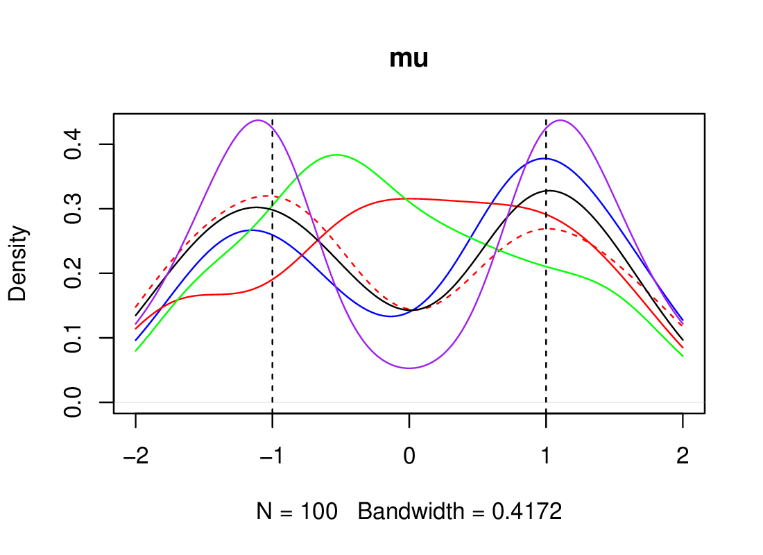
A $d = 10$ dimensional observation, simulated from a process with $ρ = 1$ , is considered. The ABC posterior distributions derived from the selected samples are shown for each of the compared procedures in Figure S9. The expectation-based summary statistics approaches (semi-automatic ABC and GLLiM-E-ABC) do not capture the bimodality. Adding the posterior log-variances (red dotted line) allows to recover the two modes. GLLiM-EV-ABC, GLLiM-MW2-ABC and GLLiM-L2-ABC provide similar bimodal posterior distributions, with more symmetry between the two modes for the two first methods.

S4 .5 Synthetic example inspired from sound source localization

In this sub-section, we consider more complex non-identifiable examples. Note that these examples are fully artificial but we explain below how they have been constructed from a real sound source localization problem in audio processing.

S4 .5.1 Two microphone setup

Although microphone arrays provide the most accurate sound source localization, setups limited to two microphones, e.g. Beal et al. (2003); Hospedales and Vijayakumar (2008), are often considered to mimic binaural hearing that resembles the human head with applications such as autonomous humanoid robot modelling. We thus first consider an artificial two microphone setup in a 2D scene. The object of interest is a sound source located at an unknown position $𝜽 = (x, y)$ . The two microphones are assumed to be located at known positions, respectively denoted by $𝒎_{1}$ and $𝒎_{2}$ . A good cue for the sound source localization is the interaural time difference (ITD) (Wang and Brown, 2006). The ITD is the difference between two times: the time a sound emitted from the source is acquired by microphone 1 at $𝒎_{1}$ and the time at microphone 2 at $𝒎_{2}$ . The function $F$ that maps a location $𝜽$ onto an ITD observation is

F (𝜽)

= \frac{1}{c} (∥ 𝜽 - 𝒎_{1} ∥_{2} - ∥ 𝜽 - 𝒎_{2} ∥_{2}),

(44)

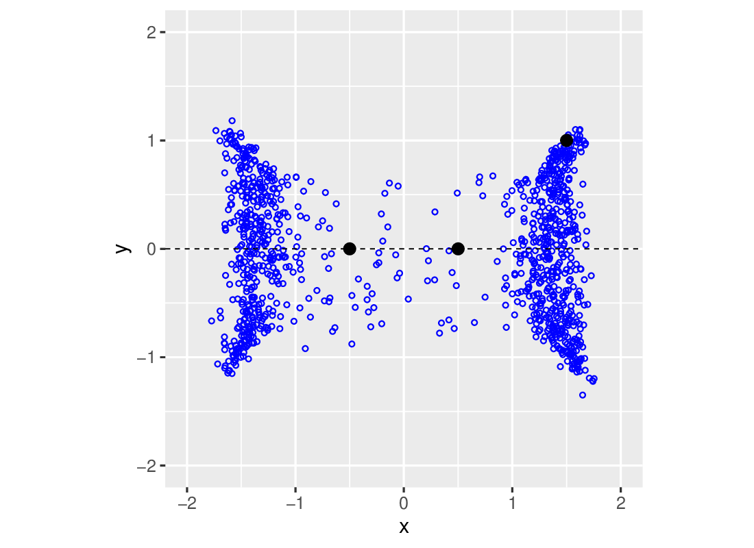
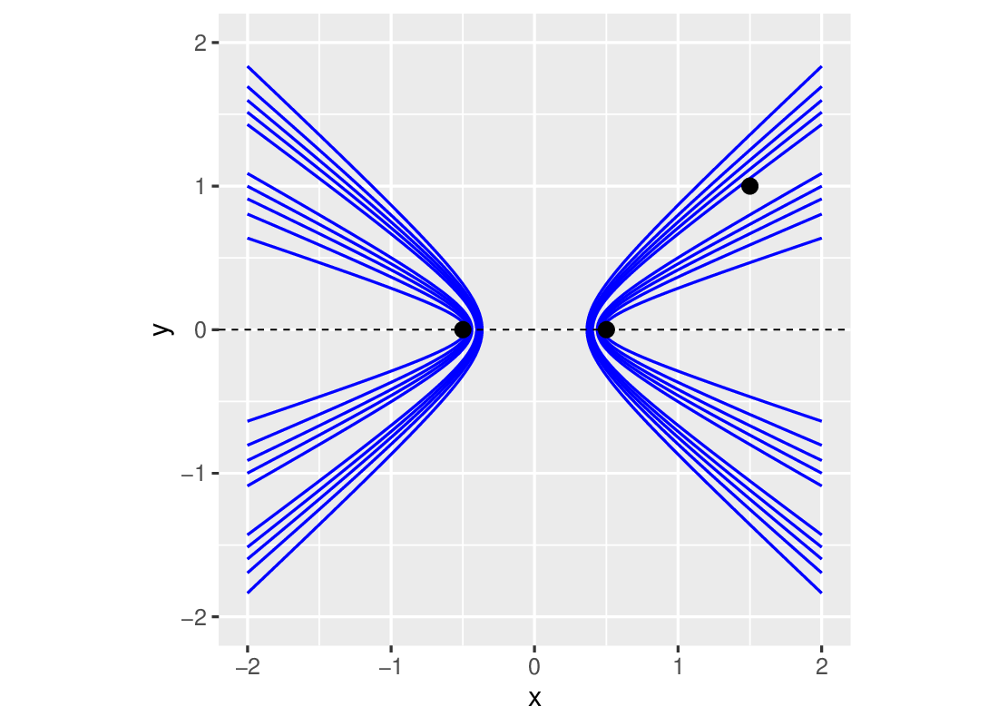
where $c$ is the sound speed in real applications but set to 1 in our example for the purpose of illustration. The important point is that an ITD value does not correspond to a unique point in the scene space, but rather to a whole surface of points. In fact, each isosurface defined by (44) is represented by one sheet of a two-sheet hyperboloid in 2D. Hence, each ITD observation constrains the location of the auditory source to lie on a 1D manifold. The corresponding hyperboloid is determined by the sign of the ITD. In our example, to create a multimodal posterior, we modify the usual setting by taking the absolute value of the ITD so that solutions can now lie on either of the two hyperboloids. In addition we assume that ITDs are observed with some Student $t$ noise that implies heavy tails and possible outliers. Although the ITD is a univariate measure, we consider a more general $d$ dimensional setting by defining the following Student $t$ likelihood, $𝐲 = (y_{1}, \dots, y_{d})$ and $ITD (𝜽) = ∣ ∥ 𝜽 - 𝒎_{1} ∥_{2} - ∥ 𝜽 - 𝒎_{2} ∥_{2} ∣$ , where

f_{𝜽} (𝐲) = 𝒮_{d} (𝐲; ITD (𝜽) 1I_{d}, σ^{2} I_{d}, ν) .

(45)

The above likelihood corresponds to a $d$ -variate Student $t$ -distribution with a $d$ -dimensional location parameter with all dimensions equal to $ITD (𝜽)$ , diagonal isotropic scale matrix equal to $σ^{2} I_{d}$ and degree-of-freedom (dof) parameter $ν$ .

The parameter space is assumed to be $Θ = [- 2, 2] \times [- 2, 2]$ and the prior on $𝜽$ is assumed to be uniform on $Θ$ . The microphones’ positions are $𝒎_{1} = (- 0.5, 0)$ and $𝒎_{2} = (0.5, 0)$ . We assume $ν = 3$ and $σ^{2} = 0.01$ . The true $𝜽$ is set to $𝜽 = (1.5, 1)$ and we simulate a 10-dimensional $𝐲$ following model (45).

The four ABC methods using GLLiM and semi-automatic ABC are compared. The semi-automatic ABC procedure uses the same data set for both the regression and rejection steps. For a fair comparison, we thus also learn here a GLLiM model from the same data set. We use a training set of $M = 10^{6}$ pairs $(𝜽, 𝐲) \in Θ \times ℝ^{10}$ , simulated from a uniform distribution on $Θ$ and applying model (45). The estimated GLLiM model consists of $K = 20$ Gaussian components with an isotropic constraint. The ABC procedures are then run on the same $M = 10^{6}$ training set. A selected set of 1000 samples is retained by thresholding the distances under the 0.1% quantile.

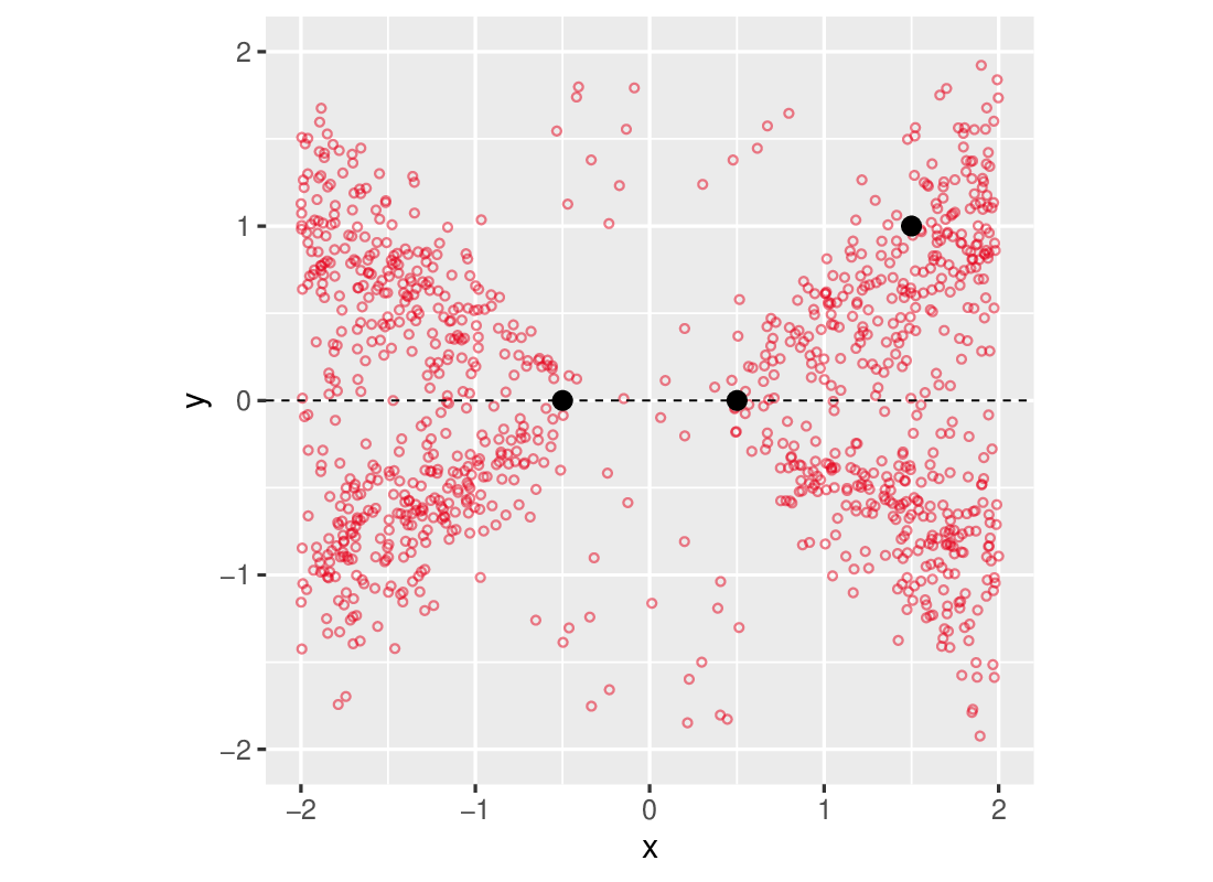
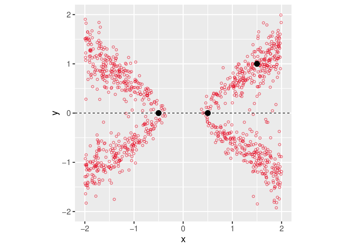
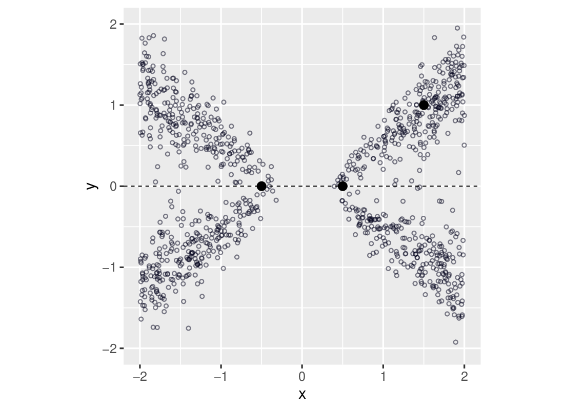
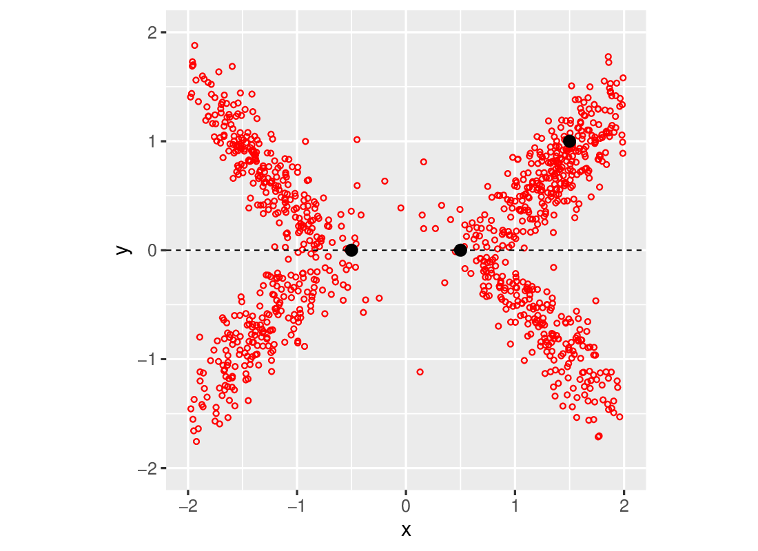
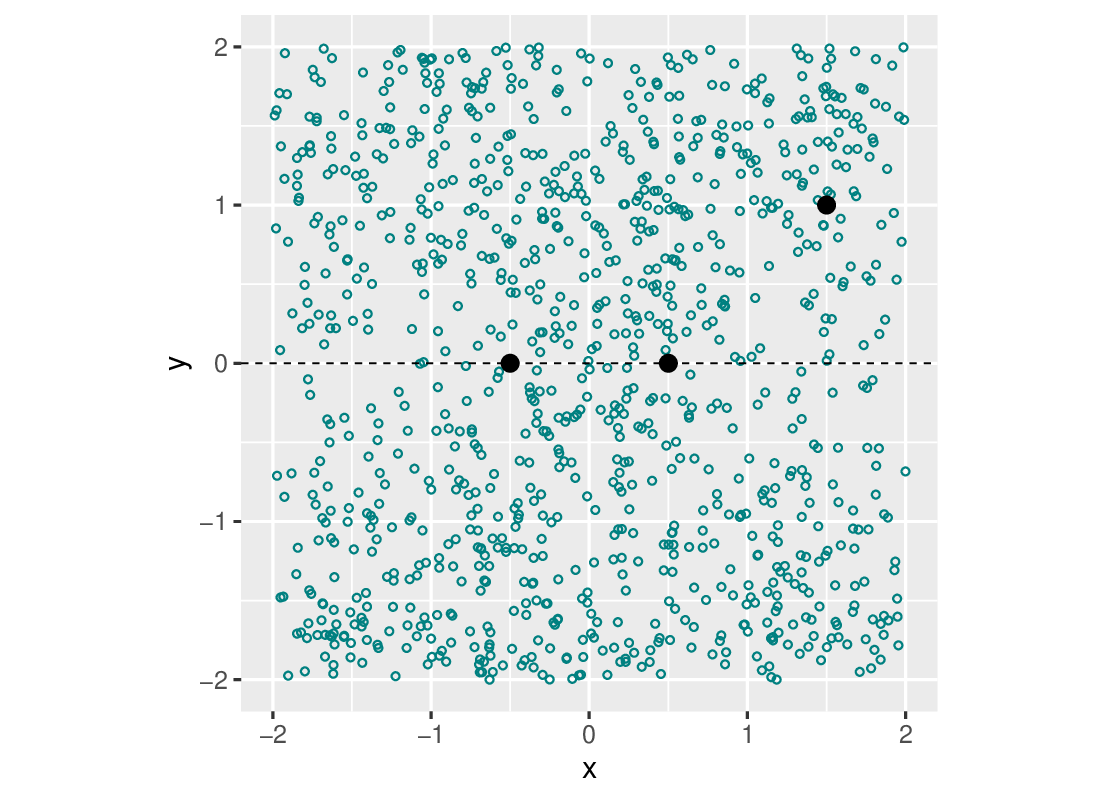
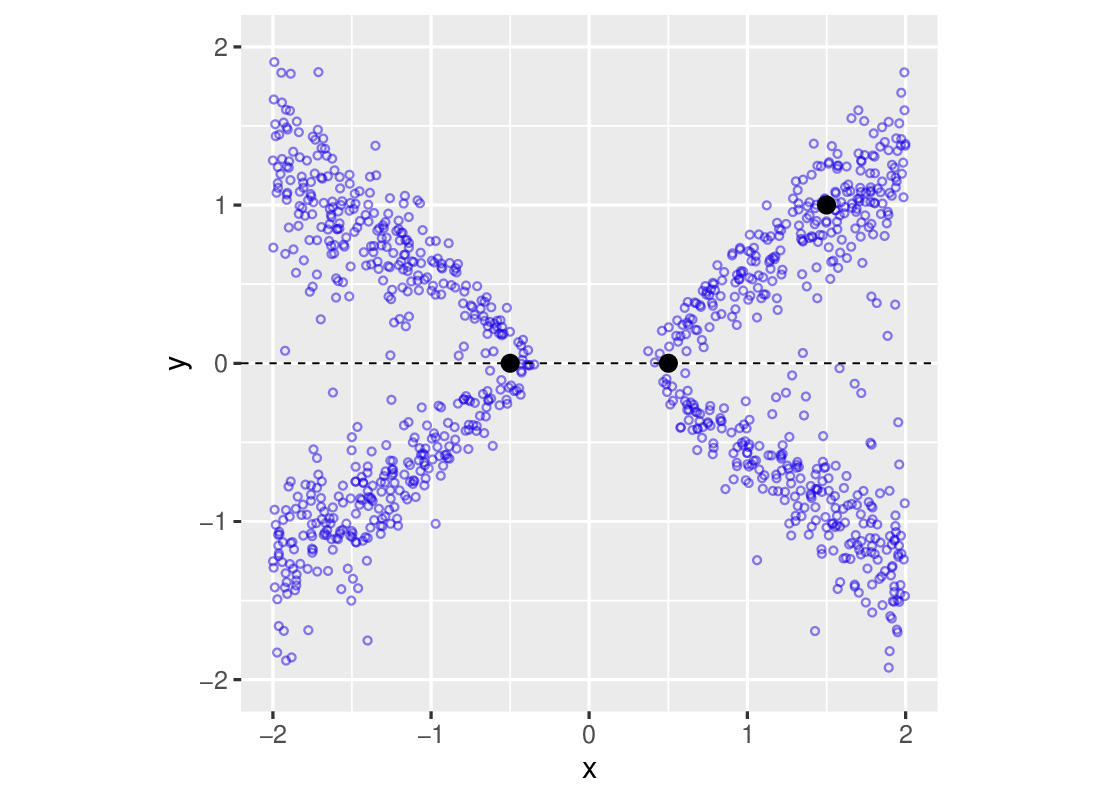
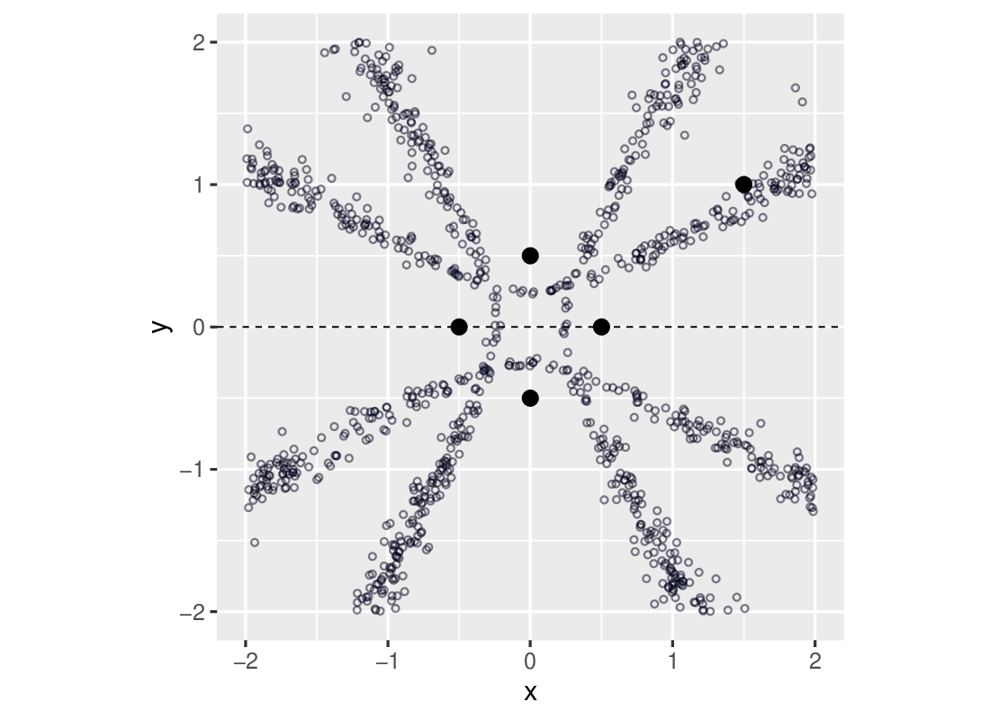
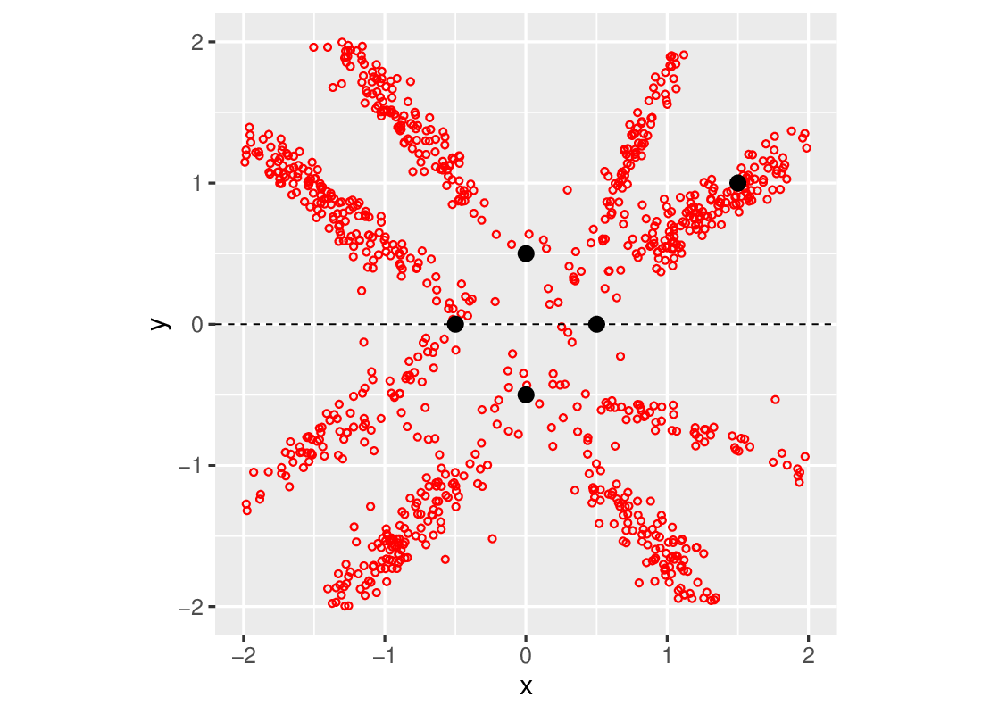
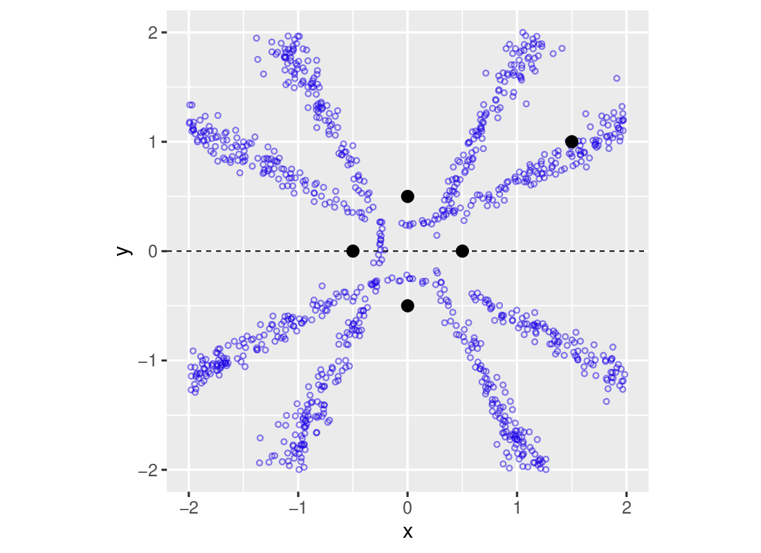
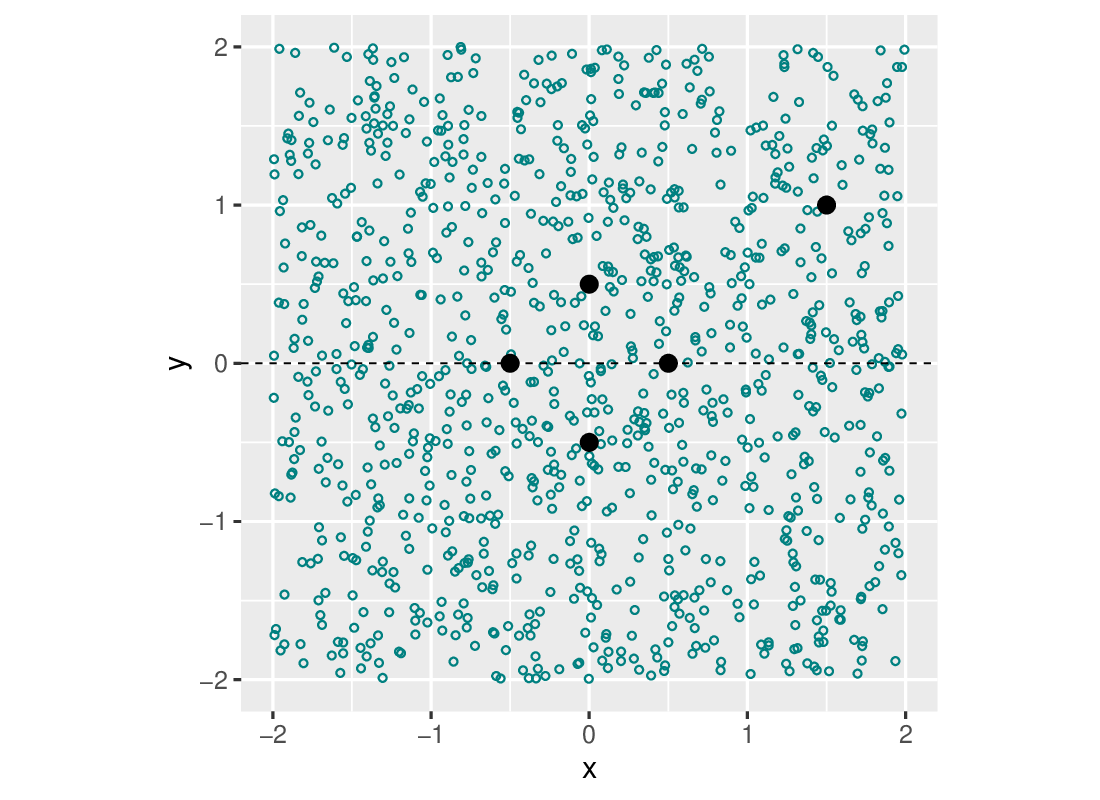
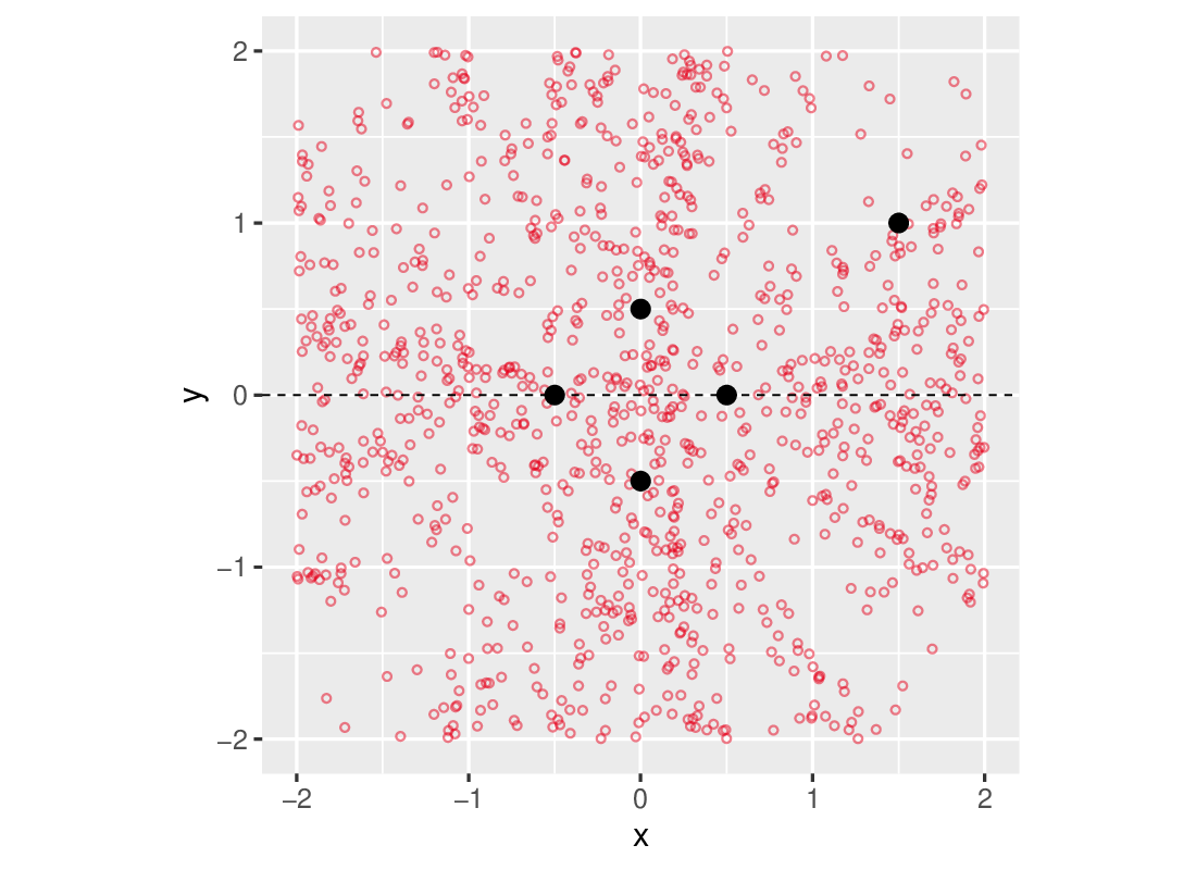
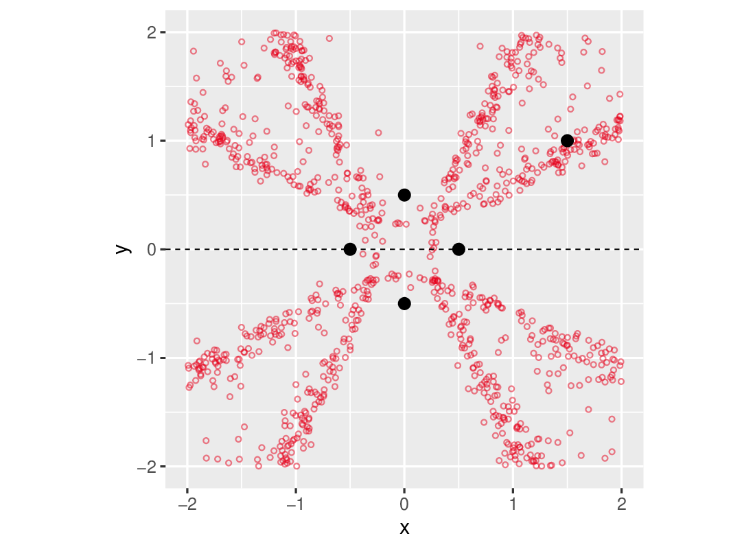
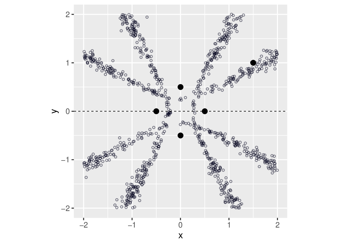
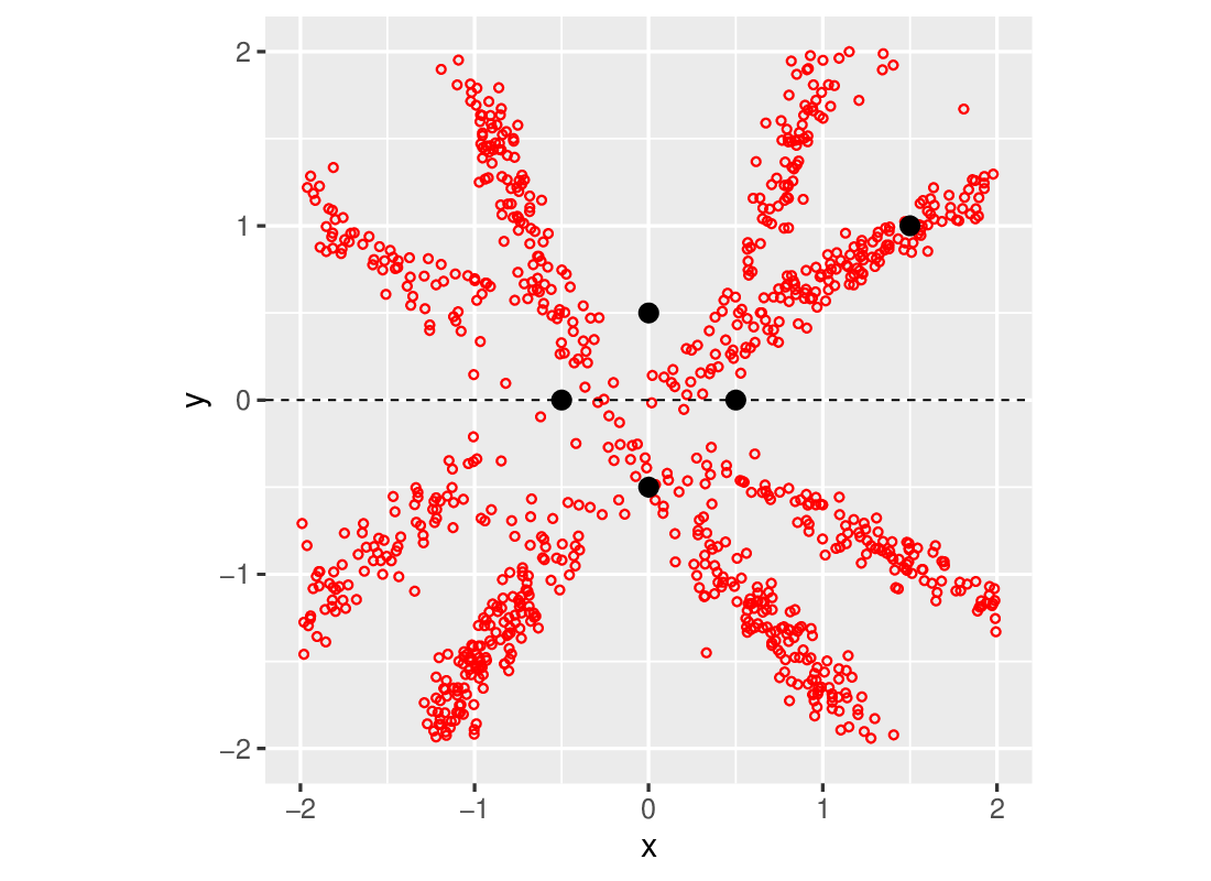
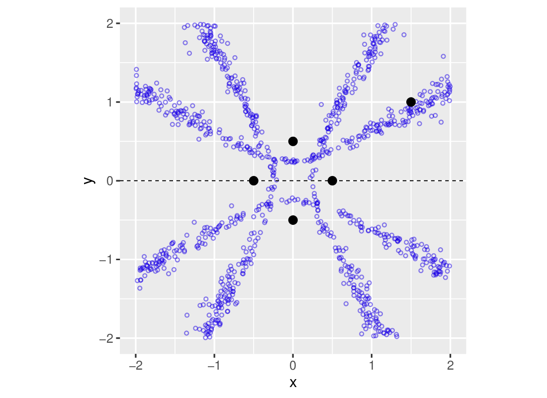
Figure S10 shows the ABC samples with another sample simulated from the GLLiM posterior distribution, corresponding to the observation $𝐲$ (Figure S10 (d)). This GLLiM posterior is a $20$ -component Gaussian mixture. Another sample obtained using the Metropolis–Hastings algorithm, as implemented in the R package mcmc (Geyer and Jonhson, 2020), is shown in Figure S10 (g)). Figure S10 (h) show the true posterior around hyperboloids, which are symmetric with respect to the microphones line and its mediatrice, and contain the true sound source localization as expected.

All tested procedures except semi-automatic ABC reflect the bimodality of the posterior distribution. The 20-component GLLiM mixture (Figure S10 (d)) reproduces correctly the bimodality of the true posterior. However, the accuracy is improved when using an additional ABC step. GLLiM-EV-ABC, GLLiM-L2-ABC and GLLiM-MW2-ABC lead to very similar selected samples (Figure S10 (b,c,f)). Using only the GLLiM posterior expectations as summary statistics is less informative although the GLLiM mixture itself appears as a reasonable approximation that well captures the main shape of the true posterior. Interestingly, semi-automatic ABC and GLLiM-E-ABC provide different selections, although both procedures are based on a preliminary estimation of the posterior means. In this example, the true posterior means are all zero due to symmetry in the posterior distributions. The semi-automatic ABC selected sample is then the one expected as the true posterior means do not carry any information on the parameter values. The posterior means approximated by GLLiM are also all around zero but the structure visible in the selected sample suggests that the surrogate means still capture some information on the parameter values, probably through the estimation bias. Paradoxically the poor semi-automatic ABC selection may be due to a more accurate preliminary regression step.

S4 .5.2 Two pairs of microphones setting

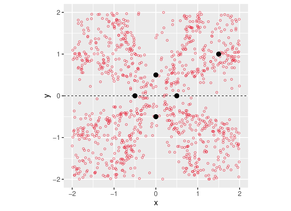
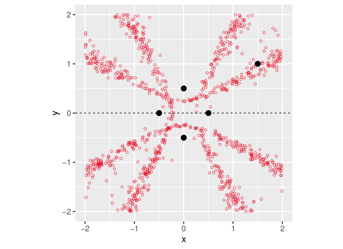
We build on the previous example to design a more complex setting. Two pairs of microphones are considered respectively located at $((- 0.5, 0), (0.5, 0))$ and $((0, - 0.5), (0, 0.5))$ . The ITD vectors are assumed to be measured with equal probability either from the first pair or from the second pair. It results a likelihood that is a mixture of two equal weight components both following the previous model but for different microphones locations. The 10-dimensional observation $𝐲$ is generated from a source at location $(1.5, 1)$ . Depending on whether this observation is coming from the first pair or second pair component, it results a true posterior as shown in Figure 1 (d) of the manuscript or one with non-intersecting hyperbolas. The contour plot indicates that the observation corresponds to the $((0, - 0.5), (0, 0.5))$ pair.

The first GLLiM model used consists of $K = 20$ Gaussian components with an isotropic constraint. A selected sample of 1000 values is retained by thresholding the distances under the $0.1 %$ quantile. In a first test, semi-automatic ABC and GLLiM use the same data set of size $M = 10^{6}$ which is also used for the rejection ABC part. Selected samples are shown Figure S11. The mixture provided by GLLiM as an approximation of the true posterior (Figure S11 (d)) well captures the main posterior parts. This GLLiM posterior is a $20$ -component Gaussian mixture. The true posterior expectations are all zero and are thus not informative about the location parameters. However, a correct structure can be seen in the GLLiM-E-ABC sample, in contrast to the semi-automatic one that shows no structure as expected. Adding the posterior log-variance estimations has a good impact on the selected sample, which is only marginally different from the GLLiM-D-ABC samples. This suggests that the posterior log-variances are very informative on the location parameters. When a larger data set with $M = 10^{6}$ is used to learn GLLiM as it is done to fit the semi-automatic ABC regression, Figure S11 shows that both GLLiM-E-ABC and GLLiM-EV-ABC improve. A more accurate GLLiM fit may therefore have an impact on this latter procedures while GLLiM-D-ABC procedures are less sensitive to the quality of the fit.

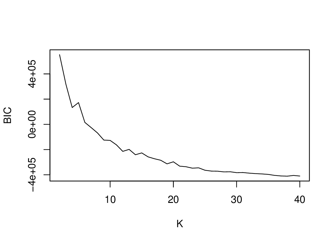
When computing BIC to select the number of components, the minimum BIC value is found for $K = 38$ . Figure S12 shows the BIC values from $K = 2$ to $K = 40$ . All GLLiM-ABC procedures are then re-ran with GLLiM learned with $K = 38$ and results are shown in Figure 1 of the manuscript. Some improvement is clearly visible compare to the $K = 20$ case.

S4 .6 Planetary science example

S4 .6.1 Selecting the number of components

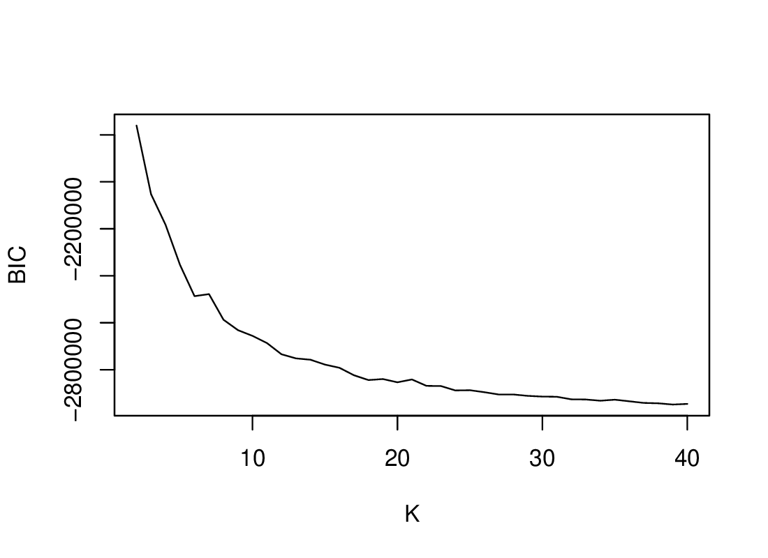
In this example, the GLLiM model is learned with $K = 40$ to be consistent with a previous study (Kugler et al., 2021). However, we checked that this number was reasonable and in particular could not be significantly reduced by computing BIC from $K = 2$ to $K = 40$ . The BIC values are shown in Figure S13. The minimum is reached for $K = 39$ but $K = 40$ provides almost the same BIC.

S4 .6.2 Synthetic data from the Hapke model

Prior to real data inversion, to illustrate the performance of the procedures, we consider an observation simulated from the Hapke model. As The Hapke model is quite difficult to invert due to equivalent solutions and low sensitivity of the model to some of the parameters. Therefore as a first validation and for a useful comparison of the procedures we chose to invert a simulated observation as close as possible to the real observed signal described in the next section. Among the simulated signals, in the ABC data set, we chose then the one whose correlation with the real observed one was the highest. This synthetic signal has been generated from the Hapke model applied to parameter values $(ω, \bar{θ}, b, c) = (0.68, 0.04, 0.23, 0.04)$ , with an additional Gaussian noise with standard deviation of 0.05.

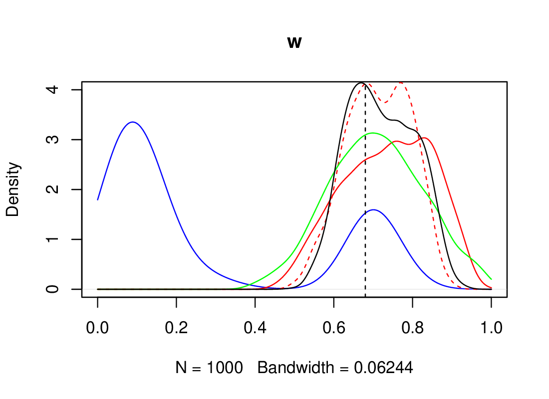
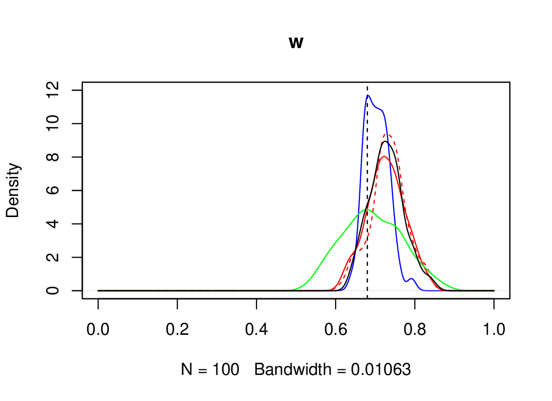
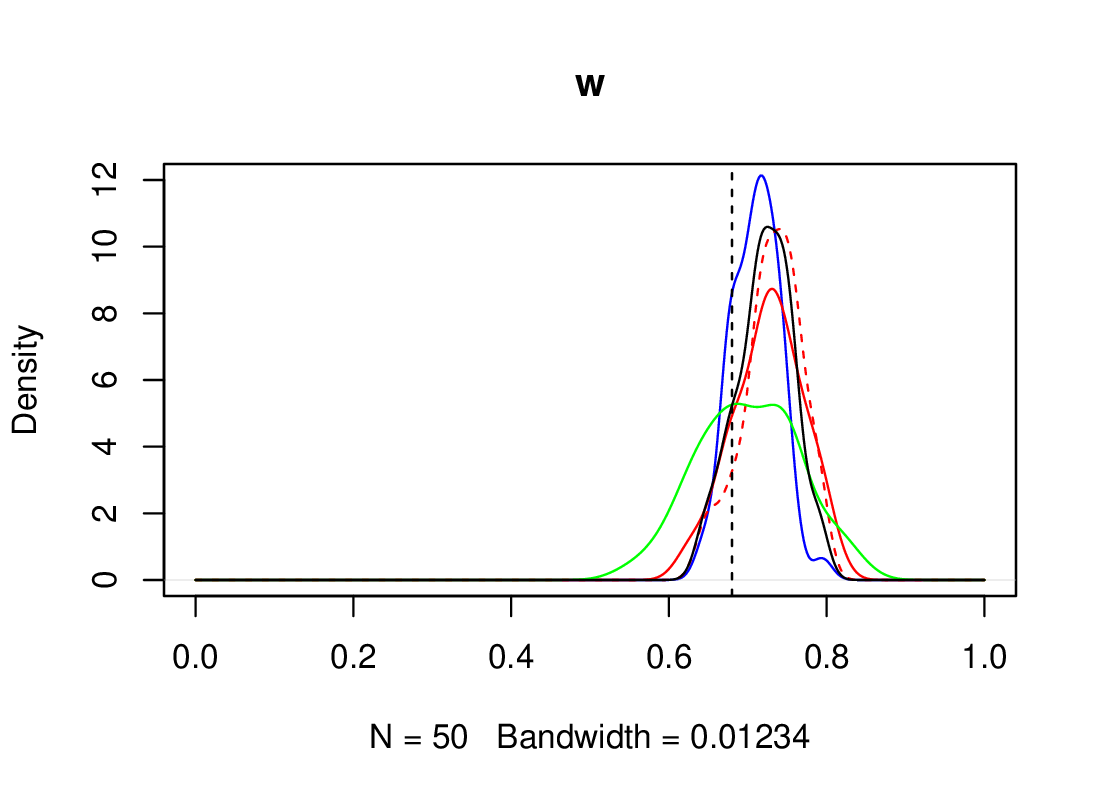
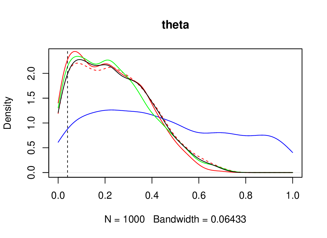
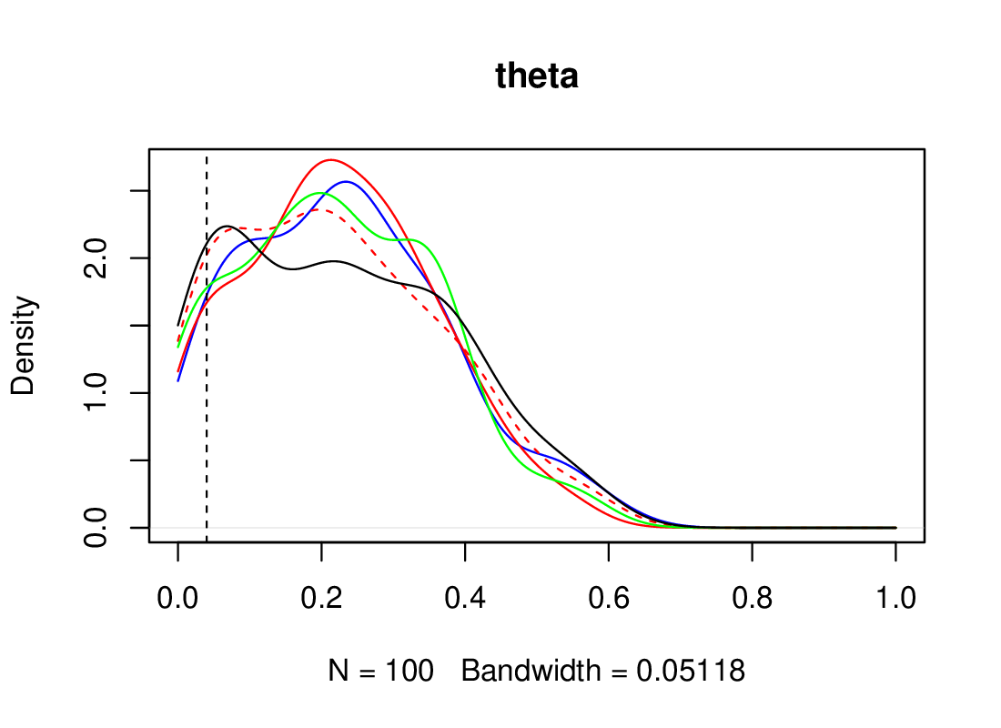
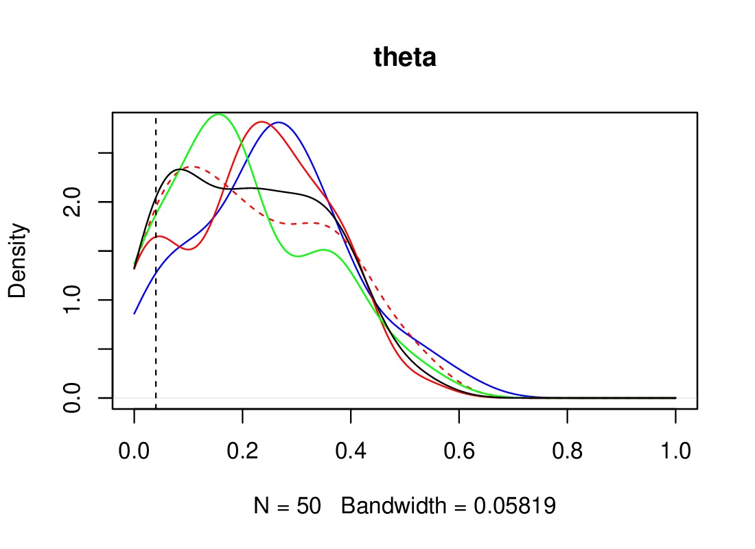
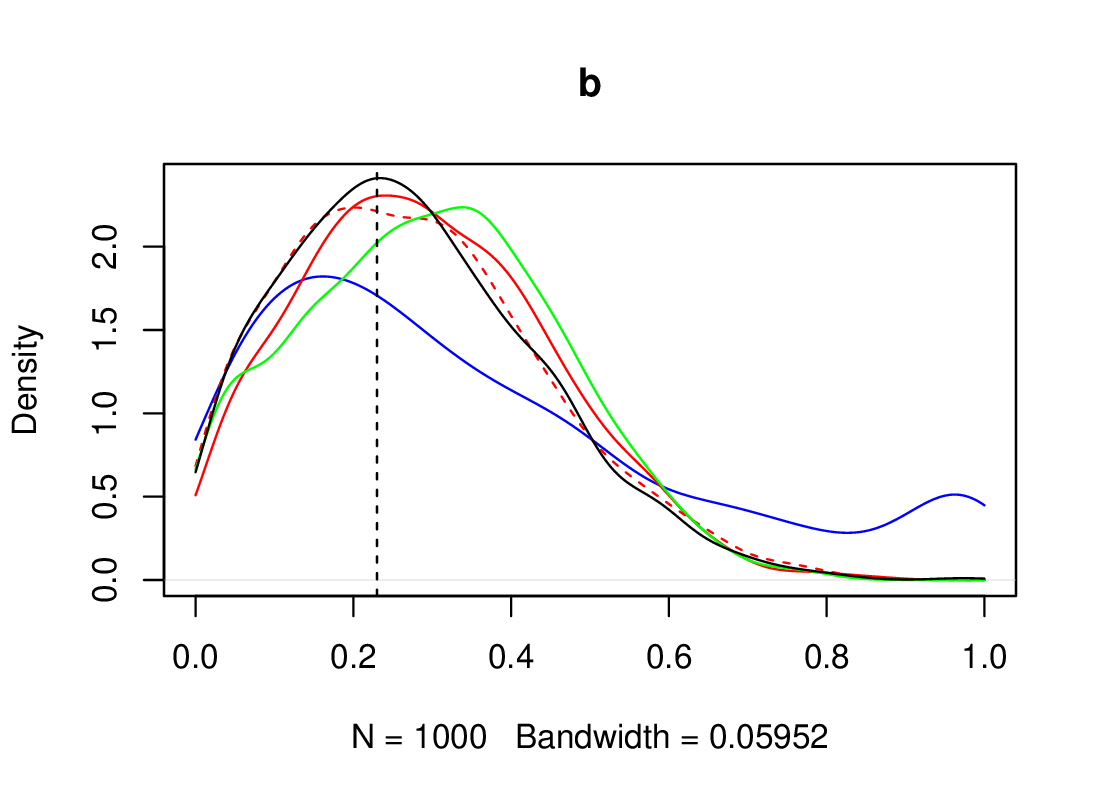
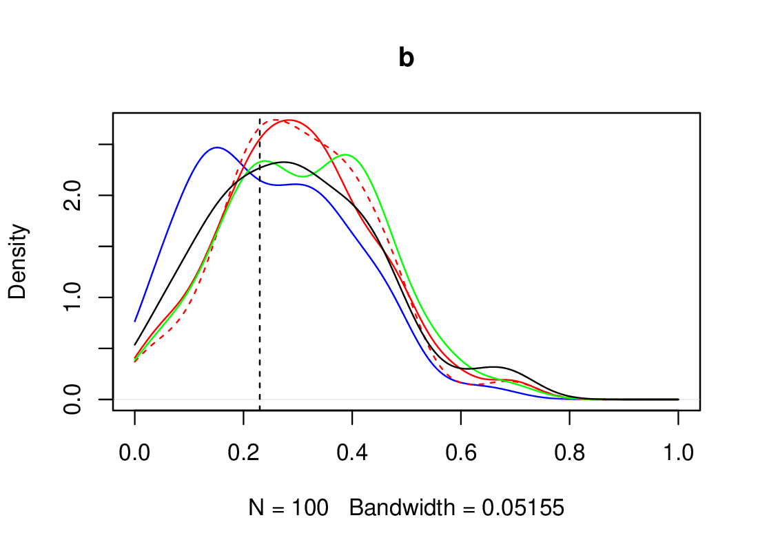
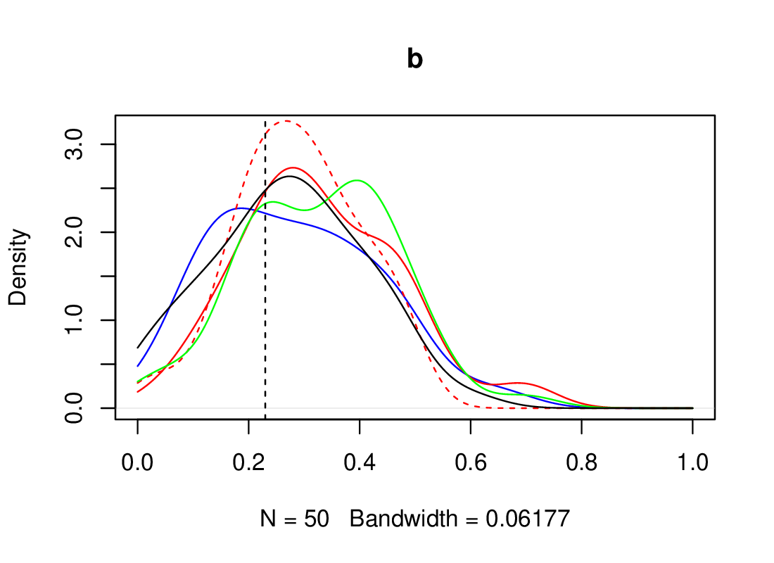
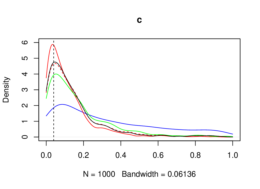
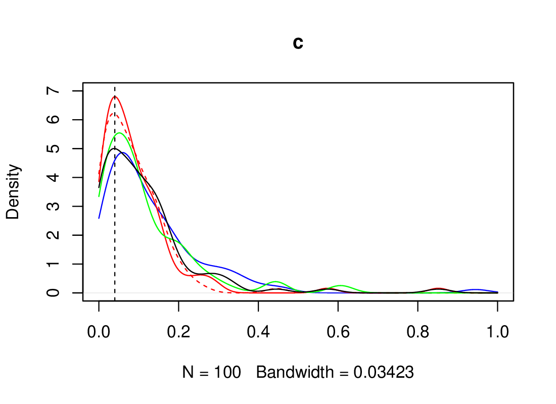
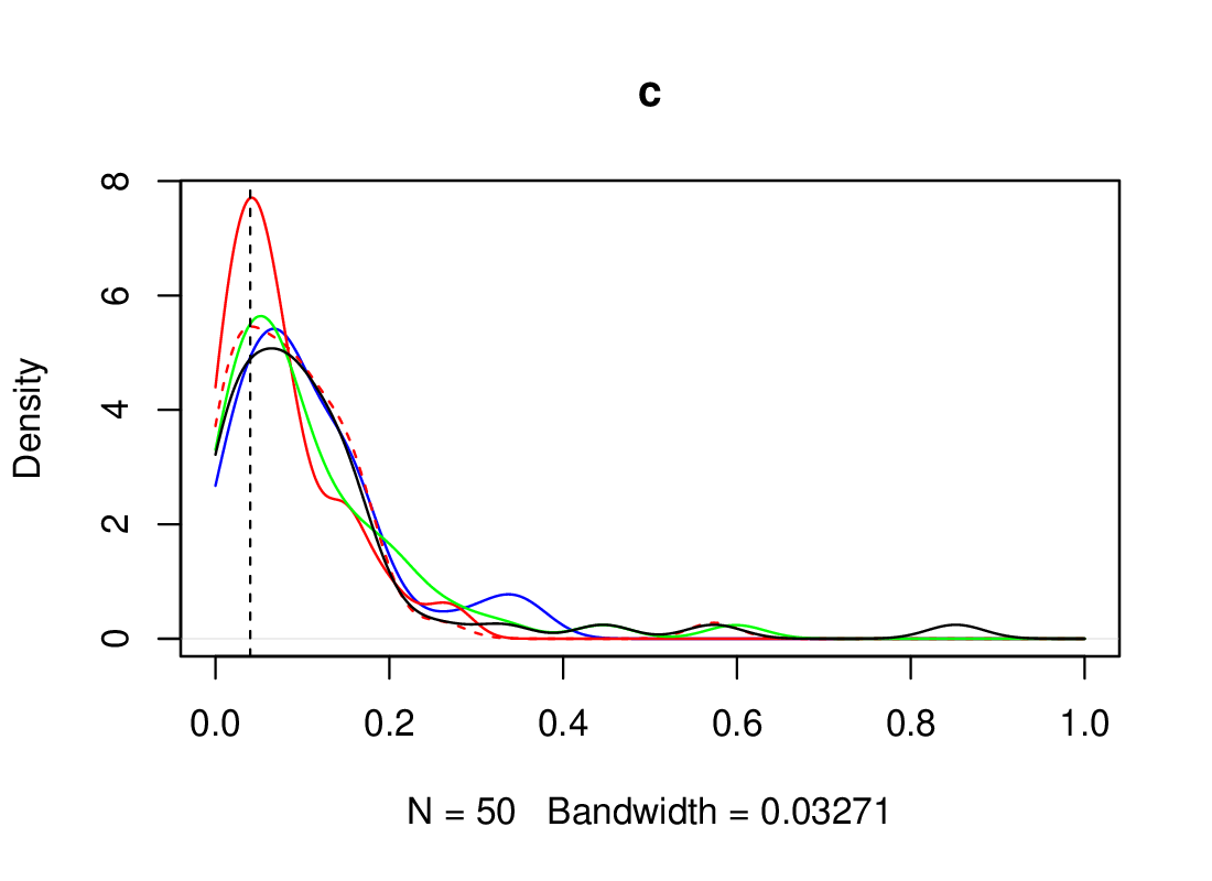
Figure S14 shows the marginal posteriors obtained for each parameter using the five ABC procedures and for different tolerance values $ϵ$ chosen as the 0.05%, 0.1% and 1% quantiles of the observed distances. A particular feature of this synthetic example is the relatively low value of $\bar{θ}$ , which does not correspond to a value expected in real data. Experts consider that reasonable values for $\bar{θ}$ are between 0.33 and 0.66 (representing in the original space an angle between 10 and 20 degrees). The Hapke model is also such that $ω$ and $\bar{θ}$ values can interact to allow the reconstruction of a given spectrum. In Figure S14, this effect is visible on the slightly shifted modes of the posterior distributions for $ω$ and $\bar{θ}$ compared to the value used for the simulation. This bias is compensating for the overly small value of $\bar{θ}$ . Then the fact that posterior distributions for $c$ are sharper than those for $b$ is also consistent with expert knowledge according to which $b$ and $\bar{θ}$ are more difficult to estimate than $ω$ and $c$ .

More generally, this example highlights the performance of the different ABC methods. It is interesting to vary $ϵ$ to observe the behavior of the different methods. A lower $ϵ$ can be used to check if one of the modes may vanish (i.e. with a more drastic thresholding) or is confirmed when the selection is more permissive. The GLLiM-L2-ABC procedure seems less robust, than the other procedures, to these variations and even degrades in performance when the thresholding is too permissive. The two procedures based on expectations as summary statistics have overall satisfying performance with globally less sharp posterior distributions. The addition of the posterior log-variances does not seem to significantly change the selected samples.

S4 .6.3 Real observation inversion

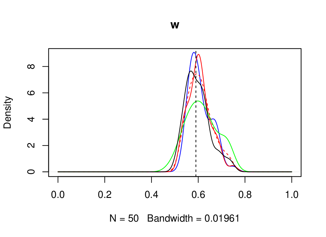
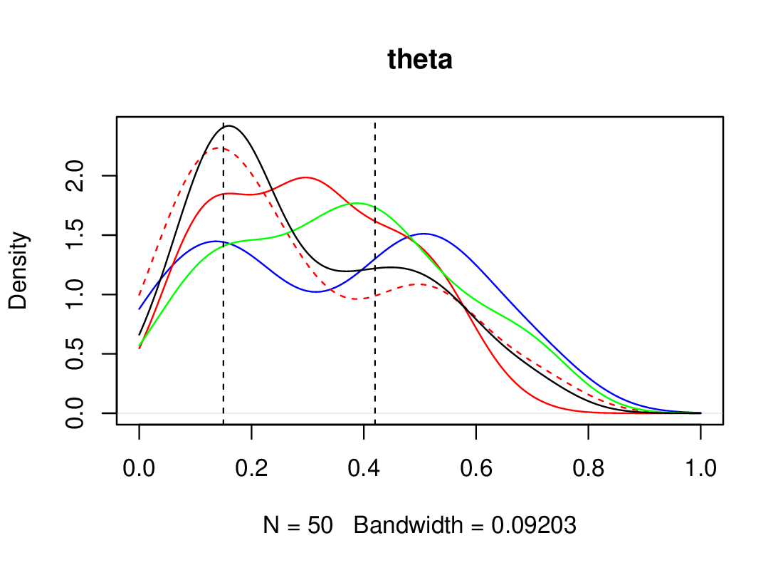
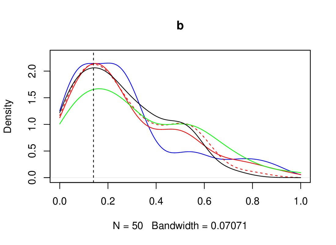
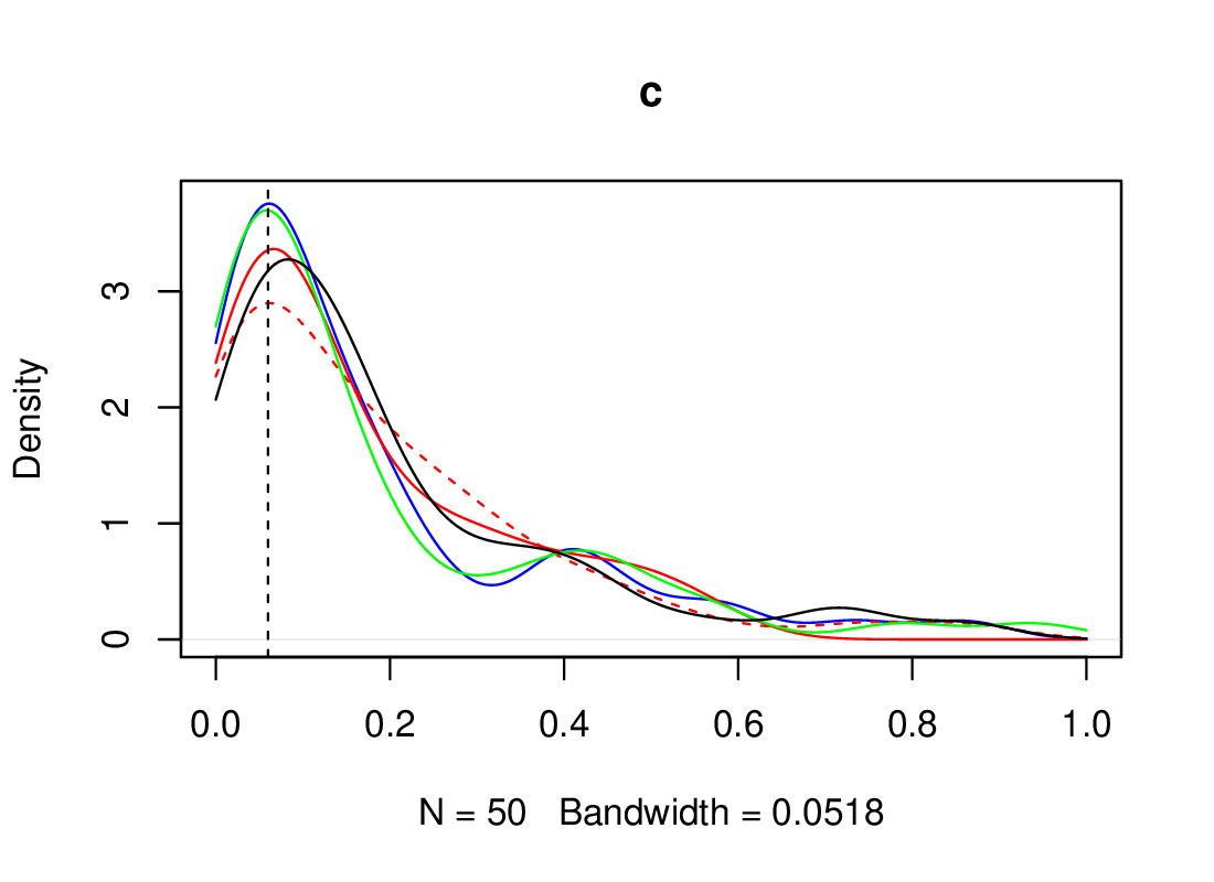
We focus on one observation coming from an experiment involving a mineral called Nontronite. The inversion described in Section 6.4 of the manuscript shows the existence of multiple solutions. A complementary test was made to check the relevance of a potential second mode observed for the $b$ parameter in Figure 2 of the manuscript. Figure S15 below, obtained by decreasing the threshold $ϵ$ to the 0.05% quantile, shows that this mode around 0.5 tends to disappear. As an additional check, the reconstructed signal obtained with this value of $b$ was observed to be quite different from the inverted signal (not shown).

S5 Computation times

Table S3 shows the settings and computation costs of the various steps for the main experiments in the manuscript. We also specify the R packages used for the various procedures, in the last column for the ABC schemes and in the first line for GLLiM and Wasserstein distances. The reported times depend to a certain extent to the packages implementations and could be in some cases improved but the overall ranking should not be too impacted. When applicable, semi-automatic ABC is always the fastest. GLLiM is always the more costly if the learning cost is included and if only one inversion is considered. The approach however could become really competitive if a large number of inversions is considered due to its amortized nature. For instance in the Bivariate Beta and MA(2) cases, GLLiM-MW2-ABC and WABC inversions takes similar times.

To improve computing time and memory usage when large datasets have to be handled, one interesting approach would be to consider stochastic, incremental or online EM algorithm implementations. Typically, online EM or online Majorization-Minimization (MM) algorithms are based, like stochastic gradient (SG), on stochastic approximation, see for instance Cappé and Moulines (2009); Mairal (2013) and some of our recent work for mixtures (Nguyen et al. (2020); Nguyen and Forbes (2022); Nguyen et al. (2022)). Although the EM algorithm is a standard approach for mixtures, mixtures can also be estimated using a standard Newton algorithm, which can itself be turned into a stochastic online procedure, see for instance Cappé and Moulines (2009). However, it is also known that the online EM algorithm is similar to a preconditioned SG using both first order and second order derivatives, and thus closer to a stochastic Newton-Raphson algorithm, and therefore can often be more efficient than SG (see an illustration in Nguyen et al. (2022)). More generally, GLLiM could be learned using gradient descent. We are not really aware of a real advantage, in general, in using the EM algorithm now that efficient numerical techniques exist to compute gradients effortlessly. However, for mixtures of Gaussians, this question has been investigated by Xu and Jordan (1996). As explained in Xu and Jordan (1996), the EM algorithm can be viewed as a variable metric gradient ascent algorithm. We refer to the conclusion in this paper for a more complete discussion. In the mixture case, one feature that is especially interesting over gradient ascent is that EM enjoys automatic satisfaction of probabilistic constraints, such as weights that sum to one, positive definite matrices, etc. and does not require the user to set a learning rate while ensuring an increasing likelihood at each step.

Exp.	ABC	$ℓ$	$d$	$K$	$N$	$M$	$R$	BIC	GLLiM	Dist.	ABC	Package
	scheme							xllim	xllim	transport
Normal	SMC-ABC
	WABC	2	2	-	-	$10^{6}$	100	-	-	-	50m	winference
	G-L2-SMC	2	2	1	$10^{5}$	$10^{6}$	100	-	-	-	2m32s	winference
	G-MW2-SMC	2	2	1	$10^{5}$	$10^{6}$	100	-	-	-	1m30s	winference
Beta	Rej-ABC
	G-E-ABC	5	2	100	$10^{5}$	$10^{5}$	100	-	11h13m	3m03s	0.28s	abc
	G-EV-ABC	5	2	100	$10^{5}$	$10^{5}$	100	-	11h13m	3m03s	0.51s	abc
	G-L2-ABC	5	2	100	$10^{5}$	$10^{5}$	100	-	11h13m	19m02s	0.01s	abc
	G-MW2-ABC	5	2	100	$10^{5}$	$10^{5}$	100	-	11h13m	19m02s	0.01s	abc
	SMC-ABC
	WABC	5	2	-	-	$10^{6}$	100	-	-	-	31m05s	winference
	G-MW2-SMC	5	2	100	$10^{5}$	$10^{6}$	100	-	11h13m	-	34m53s	winference
	G-L2-SMC	5	2	100	$10^{5}$	$10^{6}$	100	-	11h13m	-	2h34m	winference
MA(2)	Rej-ABC
	SA	2	150	-	-	$10^{5}$	1	-	-	-	1m25s	abctools
	G-E-ABC	2	30	20	$10^{5}$	$10^{5}$	5	5h46m	9m23s	50s	0.12s	abc
	G-EV-ABC	2	30	20	$10^{5}$	$10^{5}$	5	5h46m	9m23s	50s	0.20s	abc
	G-L2-ABc	2	30	20	$10^{5}$	$10^{5}$	5	5h46m	9m23s	1m03s	0.01s	abc
	G-MW2-ABC	2	30	20	$10^{5}$	$10^{5}$	5	5h46m	9m23s	1m03s	0.01s	abc
	SMC-ABC
	WABC	2	30	-	-	$10^{5}$	5	-	-	-	10m29s	winference
	G-MW2-SMC	2	30	20	$10^{5}$	$10^{5}$	5	5h46m	9m23s	-	11m08s	winference
	G-L2-SMC	2	30	20	$10^{5}$	$10^{5}$	5	5h46m	9m23s	-	8m43s	winference
Hyperb.	Rej-ABC
	SA	2	10	-	-	$10^{6}$	-	-	-	-	13s	abctools
	G-E-ABC	2	10	38	$10^{5}$	$10^{6}$	-	1h43m	4m47s	25s	0.9s	abc
	G-EV-ABC	2	10	38	$10^{5}$	$10^{6}$	-	1h43m	4m47s	11m28s	1.8s	abc
	G-L2-ABC	2	10	38	$10^{5}$	$10^{6}$	-	1h43m	4m47s	4h18m	0.1s	abc
	G-MW2-ABC	2	10	38	$10^{5}$	$10^{6}$	-	1h43m	4m47s	4h18m	0.1s	abc
	SMC-ABC
	G-MW2-SMC	2	10	38	$10^{5}$	$10^{6}$	-	1h43m	4m47s	-	1h10m	winference
Hapke	Rej-ABC
	SA	4	10	-	-	$10^{5}$	-	-	-	-	1.4s	abctools
	G-E-ABC	4	10	40	$10^{5}$	$10^{5}$	-	2h59s	21m30s	3.3s	0.2s	abc
	G-EV-ABC	4	10	40	$10^{5}$	$10^{5}$	-	2h59s	21m30s	79s	0.3s	abc
	G-L2-ABC	4	10	40	$10^{5}$	$10^{5}$	-	2h59s	21m30s	40m10s	0.01s	abc
	G-MW2-ABC	4	10	40	$10^{5}$	$10^{5}$	-	2h59s	21m30s	40m10s	0.01s	abc

Table S3: Computation times for the main experiments and procedures using rejection ABC (Rej-ABC) or SMC-ABC.

N

(resp.

M

) is the number of samples used to learn a GLLiM model (resp. for ABC). The BIC column indicates the time spent in learning all GLLiM models between

K = 2

and some

K_{max}

while the GLLiM column shows the time for the selected

K

indicated under column

K

. The Dist. column indicates, when not included in the ABC, scheme the time spent in computing all

M

distances. For GLLiM-L2-ABC and GLLiM-MW2-ABC, these distances are computed simultaneously. The indicated time is divided by two although the MW₂ distance often takes more time to compute. For semi-automatic ABC (SA) and SMC-ABC this time is included in the whole procedure time in column ABC. Different packages are used as indicated in the last column.

References

C. D. Aliprantis and K. C. Border (2006) Infinite dimensional analysis: a hitchhiker’s guide. Springer Science & Business Media. Cited by: §S3 .3.2, §S3 .3.2, §S3 .3.2, §S3 .3.2, §S3 .3.2, §S3 .3.2, §S3 .3.2. ↩ a b c d e f g h
M. J. Beal, N. Jojic, and H. Attias (2003) A graphical model for audiovisual object tracking. IEEE Trans. Pattern Anal. Mach. Intell. 25 (7), pp. 828–836. External Links: ISSN 0162-8828, Link Cited by: §S4 .5.1. ↩ a
E. Bernton, P. E. Jacob, M. Gerber, and C. P. Robert (2019) Approximate Bayesian computation with the Wasserstein distance. Journal of the Royal Statistical Society: Series B (Statistical Methodology) 81, pp. 235–269. Cited by: §S3 .1, §S4 .1, §S4 .1, §S4 .1, §S4 .2.1, §S4 .3. ↩ a b c d e f g h i
O. Cappé and E. Moulines (2009) On-line expectation-maximization algorithm for latent data models. Journal of the Royal Statistical Society B 71, pp. 593–613. Cited by: §S5. ↩ a b
Y. Chen, T. T. Georgiou, and A. Tannenbaum (2019) Optimal Transport for Gaussian Mixture Models. IEEE Access 7, pp. 6269–6278. Cited by: §S2 .1. ↩ a
R. Crackel and J. Flegal (2017) Bayesian inference for a flexible class of bivariate beta distributions. Journal of Statistical Computation and Simulation 87, pp. 295–312. Cited by: §S4 .2. ↩ a
A. Deleforge, F. Forbes, and R. Horaud (2015) High-Dimensional Regression with Gaussian Mixtures and Partially-Latent Response Variables. Statistics and Computing 25 (5), pp. 893–911. Cited by: §S1 .1, §S1 .1, §S1 .1, §S1 .1, §S1 .1, §S1. ↩ a b c d e f g h i
J. Delon and A. Desolneux (2020) A Wasserstein-type distance in the space of Gaussian Mixture Models. SIAM Journal on Imaging Sciences. Cited by: §S2 .1, §S2 .1, §S2 .1, §S2 .1. ↩ a b c d e
C. J. Geyer and L. T. Jonhson (2020) mcmc: Markov chain Monte Carlo. Note: https://cran.r-project.org/web/packages/mcmc/ Cited by: §S4 .5.1. ↩ a
T. M. Hospedales and S. Vijayakumar (2008) Structure inference for Bayesian multisensory scene understanding. IEEE Trans. Pattern Anal. Mach. Intell. 30 (12), pp. 2140–2157. External Links: ISSN 0162-8828 Cited by: §S4 .5.1. ↩ a
B. Jiang, T-Y. Wu, Z. C., and W.H. Wong (2017) Learning summary statistics for Approximate Bayesian Computation via Deep Neural Network. Statistica Sinica, pp. 1595–1618. Cited by: §S4 .3, §S4 .3. ↩ a b
B. Kugler, F. Forbes, and S. Douté (2021) Fast Bayesian Inversion for high dimensional inverse problems. To appear in Statistics and Computing, https://hal.archives-ouvertes.fr/hal-02908364. Cited by: §S4 .6.1. ↩ a
J. Mairal (2013) Stochastic majorization-minimization algorithm for large-scale optimization. In Advances in Neural Information Processing Systems, pp. 2283–2291. Cited by: §S5. ↩ a
B. Makarov and A. Podkorytov (2013) Real analysis: measures, integrals and applications. Springer Science & Business Media. Cited by: §S3 .2, §S3 .2. ↩ a b
J-M. Marin, P. Pudlo, C. P. Robert, and R. J. Ryder (2012) Approximate Bayesian computation methods. Statistics and Computing 22, pp. 1167–1180. Cited by: §S4 .4.2. ↩ a
H. D. Nguyen, F. Forbes, and G.J. McLachlan (2020) Mini-batch learning of exponential family finite mixture models. Statistics and Computing 30, pp. 731–748. Cited by: §S5. ↩ a
H.D. Nguyen and F. Forbes (2022) Global implicit function theorems and the online expectation–maximisation algorithm. Australian and New Zealand Journal of Statistics to appear. Cited by: §S5. ↩ a
H. Nguyen, F. Forbes, G. Fort, and O. Cappé (2022) An online minorization-maximization algorithm. In International Federation of Classification Societies (IFCS) conference, Cited by: §S5. ↩ a b
A. Rakhlin, D. Panchenko, and S. Mukherjee (2005) Risk bounds for mixture density estimation. ESAIM: Probability and Statistics 9, pp. 220–229. Cited by: §S3 .2, §S3 .3.1, §S3 .3.1, §S3 .3.1, Lemma 1, Lemma 1. ↩ a b c d e f
D. Schuhmacher, B. Bahre, C. Gottschlich, V. Hartmann, F. Heinemann, and B. Schmitzer (2020) transport: Computation of Optimal Transport Plans and Wasserstein Distances. Note: R package version 0.12-2 External Links: Link Cited by: §S2 .1. ↩ a
T. Tao (2011) An introduction to measure theory. American Mathematical Society Providence, RI. Cited by: §S3 .2, §S3 .2. ↩ a b c
A. B. Tsybakov (2008) Introduction to nonparametric estimation. Springer Science & Business Media. Cited by: §S3 .2. ↩ a
D. Wang and G. J. Brown (2006) Computational auditory scene analysis: principles, algorithms, and applications. Wiley-IEEE Press. External Links: ISBN 0471741094 Cited by: §S4 .5.1. ↩ a
L. Xu and M. I. Jordan (1996) On Convergence Properties of the EM Algorithm for Gaussian Mixtures. Neural Computation 8, pp. 129–151. Cited by: §S5. ↩ a b
A. J. Zeevi and R. Meir (1997) Density estimation through convex combinations of densities: approximation and estimation bounds. Neural Networks 10 (1), pp. 99–109. Cited by: §S3 .2. ↩ a

[bib.bib160] C. D. Aliprantis and K. C. Border (2006) Infinite dimensional analysis: a hitchhiker’s guide. Springer Science & Business Media. Cited by: §S3 .3.2, §S3 .3.2, §S3 .3.2, §S3 .3.2, §S3 .3.2, §S3 .3.2, §S3 .3.2. ↩ a b c d e f g h

[bib.bib71] M. J. Beal, N. Jojic, and H. Attias (2003) A graphical model for audiovisual object tracking. IEEE Trans. Pattern Anal. Mach. Intell. 25 (7), pp. 828–836. External Links: ISSN 0162-8828, Link Cited by: §S4 .5.1. ↩ a

[bib.bib27] E. Bernton, P. E. Jacob, M. Gerber, and C. P. Robert (2019) Approximate Bayesian computation with the Wasserstein distance. Journal of the Royal Statistical Society: Series B (Statistical Methodology) 81, pp. 235–269. Cited by: §S3 .1, §S4 .1, §S4 .1, §S4 .1, §S4 .2.1, §S4 .3. ↩ a b c d e f g h i

[bib.bib2] O. Cappé and E. Moulines (2009) On-line expectation-maximization algorithm for latent data models. Journal of the Royal Statistical Society B 71, pp. 593–613. Cited by: §S5. ↩ a b

[bib.bib79] Y. Chen, T. T. Georgiou, and A. Tannenbaum (2019) Optimal Transport for Gaussian Mixture Models. IEEE Access 7, pp. 6269–6278. Cited by: §S2 .1. ↩ a

[bib.bib115] R. Crackel and J. Flegal (2017) Bayesian inference for a flexible class of bivariate beta distributions. Journal of Statistical Computation and Simulation 87, pp. 295–312. Cited by: §S4 .2. ↩ a

[bib.bib98] A. Deleforge, F. Forbes, and R. Horaud (2015) High-Dimensional Regression with Gaussian Mixtures and Partially-Latent Response Variables. Statistics and Computing 25 (5), pp. 893–911. Cited by: §S1 .1, §S1 .1, §S1 .1, §S1 .1, §S1 .1, §S1. ↩ a b c d e f g h i

[bib.bib78] J. Delon and A. Desolneux (2020) A Wasserstein-type distance in the space of Gaussian Mixture Models. SIAM Journal on Imaging Sciences. Cited by: §S2 .1, §S2 .1, §S2 .1, §S2 .1. ↩ a b c d e

[bib.bib44] C. J. Geyer and L. T. Jonhson (2020) mcmc: Markov chain Monte Carlo. Note: https://cran.r-project.org/web/packages/mcmc/ Cited by: §S4 .5.1. ↩ a

[bib.bib69] T. M. Hospedales and S. Vijayakumar (2008) Structure inference for Bayesian multisensory scene understanding. IEEE Trans. Pattern Anal. Mach. Intell. 30 (12), pp. 2140–2157. External Links: ISSN 0162-8828 Cited by: §S4 .5.1. ↩ a

[bib.bib100] B. Jiang, T-Y. Wu, Z. C., and W.H. Wong (2017) Learning summary statistics for Approximate Bayesian Computation via Deep Neural Network. Statistica Sinica, pp. 1595–1618. Cited by: §S4 .3, §S4 .3. ↩ a b

[bib.bib85] B. Kugler, F. Forbes, and S. Douté (2021) Fast Bayesian Inversion for high dimensional inverse problems. To appear in Statistics and Computing, https://hal.archives-ouvertes.fr/hal-02908364. Cited by: §S4 .6.1. ↩ a

[bib.bib6] J. Mairal (2013) Stochastic majorization-minimization algorithm for large-scale optimization. In Advances in Neural Information Processing Systems, pp. 2283–2291. Cited by: §S5. ↩ a

[bib.bib158] B. Makarov and A. Podkorytov (2013) Real analysis: measures, integrals and applications. Springer Science & Business Media. Cited by: §S3 .2, §S3 .2. ↩ a b

[bib.bib145] J-M. Marin, P. Pudlo, C. P. Robert, and R. J. Ryder (2012) Approximate Bayesian computation methods. Statistics and Computing 22, pp. 1167–1180. Cited by: §S4 .4.2. ↩ a

[bib.bib3] H. D. Nguyen, F. Forbes, and G.J. McLachlan (2020) Mini-batch learning of exponential family finite mixture models. Statistics and Computing 30, pp. 731–748. Cited by: §S5. ↩ a

[bib.bib4] H.D. Nguyen and F. Forbes (2022) Global implicit function theorems and the online expectation–maximisation algorithm. Australian and New Zealand Journal of Statistics to appear. Cited by: §S5. ↩ a

[bib.bib5] H. Nguyen, F. Forbes, G. Fort, and O. Cappé (2022) An online minorization-maximization algorithm. In International Federation of Classification Societies (IFCS) conference, Cited by: §S5. ↩ a b

[bib.bib157] A. Rakhlin, D. Panchenko, and S. Mukherjee (2005) Risk bounds for mixture density estimation. ESAIM: Probability and Statistics 9, pp. 220–229. Cited by: §S3 .2, §S3 .3.1, §S3 .3.1, §S3 .3.1, Lemma 1, Lemma 1. ↩ a b c d e f

[bib.bib42] D. Schuhmacher, B. Bahre, C. Gottschlich, V. Hartmann, F. Heinemann, and B. Schmitzer (2020) transport: Computation of Optimal Transport Plans and Wasserstein Distances. Note: R package version 0.12-2 External Links: Link Cited by: §S2 .1. ↩ a

[bib.bib54] T. Tao (2011) An introduction to measure theory. American Mathematical Society Providence, RI. Cited by: §S3 .2, §S3 .2. ↩ a b c

[bib.bib53] A. B. Tsybakov (2008) Introduction to nonparametric estimation. Springer Science & Business Media. Cited by: §S3 .2. ↩ a

[bib.bib70] D. Wang and G. J. Brown (2006) Computational auditory scene analysis: principles, algorithms, and applications. Wiley-IEEE Press. External Links: ISBN 0471741094 Cited by: §S4 .5.1. ↩ a

[bib.bib14] L. Xu and M. I. Jordan (1996) On Convergence Properties of the EM Algorithm for Gaussian Mixtures. Neural Computation 8, pp. 129–151. Cited by: §S5. ↩ a b

[bib.bib57] A. J. Zeevi and R. Meir (1997) Density estimation through convex combinations of densities: approximation and estimation bounds. Neural Networks 10 (1), pp. 99–109. Cited by: §S3 .2. ↩ a

	$\| q_{ϵ} (𝜽 ∣ 𝐲) - π (𝜽 ∣ 𝐲) \|$	$\leq \int_{𝒴} K_{ϵ} (𝐳; 𝐲) \| π (𝜽 ∣ 𝐳) - π (𝜽 ∣ 𝐲) \| d 𝐳$
		$\leq sup_{𝐳 \in A_{ϵ}} \| π (𝜽 ∣ 𝐳) - π (𝜽 ∣ 𝐲) \|$
		$= \| π (𝜽 ∣ 𝐳_{ϵ}) - π (𝜽 ∣ 𝐲) \|,$

	$D_{H}^{2} (q_{ϵ}^{K, N} (\cdot ∣ 𝐲), π (\cdot ∣ 𝐲))$	$\leq D_{1} (q_{ϵ}^{K, N} (\cdot ∣ 𝐲), π (\cdot ∣ 𝐲))$
		$= \int_{Θ} \| q_{ϵ}^{K, N} (𝜽 ∣ 𝐲) - π (𝜽 ∣ 𝐲) \| d λ (𝜽)$
		$\leq \int_{Θ} \int_{𝒴} K_{ϵ}^{K, N} (𝐳; 𝐲) \| π (𝜽 ∣ 𝐳) - π (𝜽 ∣ 𝐲) \| d λ (𝐳) d λ (𝜽)$
		$= \int_{𝒴} K_{ϵ}^{K, N} (𝐳; 𝐲) \int_{Θ} \| π (𝜽 ∣ 𝐳) - π (𝜽 ∣ 𝐲) \| d λ (𝜽) d λ (𝐳)$
		$\leq sup_{𝐳 \in A_{ϵ, 𝐲}^{K, N}} \int_{Θ} \| π (𝜽 ∣ 𝐳) - π (𝜽 ∣ 𝐲) \| d λ (𝜽) .$


(a) GLLiM mixture ( $K = 20$ )	(b) Semi-automatic ABC	(c) Auto-covariances	(d) SA auto-covariances

(e) GLLiM-E-ABC ( $K = 30$ )	(f) GLLiM-EV-ABC ( $K = 30$ )	(g) GLLiM-L2-ABC ( $K = 30$ )	(h) GLLiM-MW2-ABC ( $K = 30$ )

(i) GLLiM-E-ABC ( $K = 20$ )	(j) GLLiM-EV-ABC ( $K = 20$ )	(k) GLLiM-L2-ABC ( $K = 20$ )	(l) GLLiM-MW2-ABC ( $K = 20$ )

	(m) WABC	(n) GLLiM-L2-SMC ( $K = 20$ )	(o) GLLiM-MW2-SMC ( $K = 20$ )


(a) GLLiM-E-ABC	(b) GLLiM-EV-ABC	(c) GLLiM-MW2-ABC

(d) GLLiM mixture	(e) Semi-automatic ABC	(f) GLLiM-L2-ABC

(g) Metropolis-Hastings	(h) True posterior


(a) GLLiM-E-ABC	(b) GLLiM-EV-ABC	(c) GLLiM-MW2-ABC

(d) GLLiM mixture	(e) GLLiM-L2-ABC	(f) Semi-automatic ABC

(g) GLLiM-E-ABC	(h) GLLiM-EV-ABC	(i) GLLiM-MW2-ABC

(j) GLLiM mixture	(k) GLLiM-L2-ABC





(a) 1% (1000 samples)	(b) 0.1% (100 samples)	(c) 0.05% (50 samples)