FACET: A Fragment-Aware Conformer Ensemble Transformer

Duy M. H. Nguyen; Trung Q. Nguyen; Ha T. H. Le; Mai Thanh Nhat Truong; TrungTin Nguyen; Nhat Ho; Khoa D. Doan; Duy Duong-Tran; Li Shen; Daniel Sonntag; James Zou; Mathias Niepert; Hyojin Kim; Jonathan E. Allen

Abstract

Accurately predicting molecular properties requires effective integration of structural information from both 2D molecular graphs and their corresponding equilibrium conformer ensembles. In this work, we propose a scalable Structure-Aware Graph Transformer that efficiently aggregates features from multiple 3D conformers while incorporating fragment-level information from 2D graphs. Unlike prior methods that depend on static geometric solvers or rigid fusion strategies, our approach employs a trainable attention-based mechanism within a graph transformer to dynamically fuse 2D and 3D representations. We further enhance this mechanism by injecting fragment-specific structural biases into the attention layers, enabling the model to capture fine-grained molecular details. Our method scales to large datasets, handling up to 75,000 molecules and hundreds of thousands of conformers, and achieves state-of-the-art results in molecular property prediction and reaction-level modeling. It is particularly effective on chemically diverse compounds, including organocatalysts and transition-metal complexes.

1 Introduction

Machine learning has become a powerful tool for predicting molecular properties, with wide-ranging applications in drug discovery and materials science (Choudhary et al., 2022; Fedik et al., 2022; Batatia et al., 2023). Most existing models rely either on 2D molecular graphs, which efficiently capture topological connectivity (Xu et al., 2018; Veličković et al., 2018), or on 3D representations derived from a single conformer (Schütt et al., 2017; Batzner et al., 2022; Batatia et al., 2022). While 2D graphs are computationally efficient, they lack geometric information that is often critical for accurate property prediction. Incorporating 3D conformers helps address this by introducing spatial features such as bond lengths, and torsion angles. However, relying on a single conformer still fails to capture the intrinsic flexibility of molecular structures.

In reality, molecules dynamically sample a range of thermodynamically accessible conformations due to bond rotations, vibrations, and environmental interactions (Ramsundar et al., 2019). As a result, many experimentally observable properties such as solubility and binding affinity depend on the full ensemble of conformers a molecule can adopt (Perola & Charifson, 2004). Yet, fully modeling this distribution is computationally prohibitive, as generating and evaluating large numbers of conformers using quantum methods is costly (Medrano Sandonas et al., 2024). This has motivated hybrid models that combine the structural efficiency of 2D graphs with the geometric richness of a small and representative subset of 3D conformers. By jointly capturing topological and spatial variation, hybrid models offer scalable and expressive frameworks for molecular representation, enabling more accurate prediction of conformation-sensitive properties across a range of chemical and biological tasks.

Building on this hybrid paradigm, recent methods have introduced hybrid models that integrate 2D molecular graphs with 3D conformer information to capture both topological and spatial features (Zhu et al., 2024b; Axelrod & Gomez-Bombarelli, 2023). Despite the successes, these methods often assume conformers contribute equally or can be reweighted without considering deeper geometric context. In practice, only a subset of conformers may be thermodynamically or functionally relevant, and naive aggregation overlooks their spatial relationships, such as alignment or structural similarity. Moreover, current strategies rarely leverage interactions between 2D structural priors and 3D conformational variability, hindering the formation of truly expressive representations.

To address this, structure-aware ensemble methods based on optimal transport, especially those using fused Gromov-Wasserstein (FGW) alignment, have shown promise Ma et al. (2023); Nguyen et al. (2024a). By aligning both feature and geometric spaces, these models better preserve spatial correspondences across conformers and enable expressive ensemble aggregation. However, such methods are computationally expensive and struggle to scale to large molecular datasets such as Drugs-75k Zhu et al. (2023); Axelrod & Gomez-Bombarelli (2022), limiting their utility for high-throughput applications in generative biology.

To address scalability challenges in geometry-aware molecular modeling, we introduce a novel approach that replaces expensive FGW alignment with efficient attention-based conformer aggregation. By supervising the model with FGW distances during training, we learn a latent embedding space where conformer similarities reflect both topological and geometric structure. This enables fast, permutation-invariant conformer integration suitable for large-scale generative pipelines. Beyond efficiency, we further enrich our model with fragment-level structural priors from 2D molecular graphs, injecting chemically meaningful hierarchies into both message passing and 3D attention layers. This unified 2D–3D framework captures fine-grained spatial and topological interactions essential for applications such as molecular property prediction, virtual screening, and functional optimization. In summary, our key contributions are:

•

We propose a scalable, geometry-aware conformer aggregation framework, denoted as FACET, that replaces costly FGW alignment with a trainable Graph Transformer, enabling efficient, deterministic attention-based inference. We further provide theoretical bounds on the approximation error relative to FGW distances.
•

We introduce a unified 2D–3D representation learning approach that embeds fragment-level structural priors into both 2D message passing and 3D spatial self-attention, capturing multi-scale interactions between molecular topology and geometry.
•

Our method delivers over $6 \times$ faster aggregation than prior geometry-aware baselines and achieves state-of-the-art performance across six benchmarks, including molecular property prediction and Boltzmann-weighted ensemble tasks, demonstrating robustness across diverse molecular scenarios and dataset scales.

2 Related Work

2.1 Conformer Ensemble Learning in Molecular Representations

Traditional molecular representations span connectivity fingerprints (Morgan, 1965), 1D string encodings (Ahmad et al., 2022; Wang et al., 2019), 2D topological graphs (Yang et al., 2019a; Rong et al., 2020), and 3D geometric graphs (Fang et al., 2021; Zhou et al., 2023). 3D models typically rely on a single conformer, overlooking the fact that molecules often adopt multiple low-energy conformations, which can serve as informative features, particularly in capturing thermodynamic properties. Hybrid approaches now combine 2D graphs with ensembles of 3D conformers (Zhu et al., 2024b; Wang et al., 2024), aggregated via mean pooling, DeepSets (Zaheer et al., 2017), or self-attention (Vaswani et al., 2017). More advanced geometry-aware methods based on Fused Gromov-Wasserstein (FGW) alignment (Ma et al., 2023; Nguyen et al., 2024a) capture both feature and structural similarity across conformers, but remain computationally costly and scale poorly to large datasets (e.g., Drugs-75k) or foundation models (Zhou et al., 2023; Chithrananda et al., 2020). To address this, we propose a scalable framework that learns latent embeddings of 3D conformers with graph transformers, integrating geometry-aware signals inspired by FGW and hierarchical fragment-level features. This yields a permutation-invariant, expressive, and efficient method.

2.2 Scalable Optimal Transport for Graph Learning

Learning-based approximations of Optimal Transport (OT) have emerged as efficient alternatives to traditional solvers. Early works introduced differentiable Sinkhorn distances with entropic regularization for stability and scalability (Cuturi, 2013; Feydy et al., 2019; Genevay et al., 2018). Later methods improved efficiency via structural assumptions - e.g., low-rank factorization (Scetbon et al., 2021; Cuturi et al., 2020) and spatial geometry (Bachmann et al., 2022; Solomon et al., 2015). Meta-learning approaches further accelerated convergence by learning initialization schemes (Amos et al., 2023). More recently, neural OT surrogates trained directly on data have bypassed iterative solvers entirely (Courty et al., 2017; Tong et al., 2021; Haviv et al., 2024).

However, prior works focus on standard OT and fail to extend to structure-aware variants like FGW, which jointly capture node attributes and graph topology. To address this, we introduce the first learned approximation of FGW with a graph transformer, enabling scalable, geometry-aware conformer aggregation. By embedding fragment-level priors into both 2D and 3D encoders, our approach supports multi-scale reasoning across topological and spatial hierarchies, effectively bridging molecular graphs with 3D conformational diversity.

2.3 Fragment-biases in Molecular GNN

Fragment-level substructures - such as rings, functional groups, and pharmacophores - are key to molecular property prediction and drug design (Merlot et al., 2003; Varnek et al., 2005). Recent works have leveraged these motifs for scaffold-aware drug discovery (Lee et al., 2024; Chan et al., 2024), self-supervised learning via fragment-based masking or contrastive tasks (Rong et al., 2020; Zhang et al., 2021; Wen et al., 2024), and GNN architectures that encode fragment-level inductive biases (Wang et al., 2025; Wollschläger et al., 2024). These methods show that fragments enhance generalization, interpretability, and data efficiency. Building on these insights, we explore a complementary direction: integrating fragment-level priors into hybrid 2D–3D ensemble models. In our approach, fragment hierarchies are embedded into both 2D message-passing and 3D spatial attention layers, enabling multi-scale processing across molecular topology and geometry. This design improves conformer aggregation and yields more expressive, geometry-aware representations suited for conformation-sensitive tasks.

3 Fragment-Aware Conformer Ensemble Transformer

Notation. Let $Δ_{N} : = {𝝎 \in ℝ_{+}^{N} : 𝝎^{⊤} 𝟏_{N} = 1}$ denote the probability simplex, where $𝟏_{N}$ is the all-ones vector in $ℝ^{N}$ . For $x \in 𝛀$ , $δ_{x}$ is the Dirac measure at $x$ . We write $[K] : = {1, \dots, K}$ for $K \in ℕ$ , and use $⟨ \cdot, \cdot ⟩$ to denote the Frobenius inner product. For a tensor $𝑳 = (L_{i j k l})$ and matrix $𝑩 = (B_{k l})$ , define the contraction $𝑳 \otimes 𝑩 : = (\sum_{k l} L_{i j k l} B_{k l})_{i j}$ . A graph $G = (V, E)$ has $N : = | V |$ nodes and edges $E \subseteq {{u, v} \subseteq V : u \neq v}$ . An attributed graph is given by $𝒢 : = (𝑯, 𝑨, 𝝎)$ , where $𝑯 \in ℝ^{N \times d}$ is the node feature matrix (with row $𝑯_{v}$ for node $v$ ), $𝑨 \in ℤ^{N \times N}_{+}$ encodes structure (e.g., adjacency or shortest-path distance matrix), and $𝝎 \in Δ_{N}$ is a node weight distribution.

Given two graphs $𝒢_{1}$ and $𝒢_{2}$ with $N_{1}$ and $N_{2}$ nodes, the Fused Gromov-Wasserstein (FGW) distance (Peyré et al., 2016; Titouan et al., 2019, 2020) is: $FGW_{p, α} (𝒢_{1}, 𝒢_{2}) : = \min_{𝝅 \in Π (𝝎_{1}, 𝝎_{2})} ⟨ (1 - α) 𝑴 + α 𝑳 (𝑨_{1}, 𝑨_{2}) \otimes 𝝅, 𝝅 ⟩,$ where $Π (𝝎_{1}, 𝝎_{2}) : = {𝝅 \in ℝ_{+}^{N_{1} \times N_{2}} : 𝝅 𝟏_{N_{2}} = 𝝎_{1}, 𝝅^{⊤} 𝟏_{N_{1}} = 𝝎_{2}}$ is the set of valid couplings, $𝑴 [i, j] = d_{f} (𝑯_{1} [i], 𝑯_{2} [j])^{p}$ is the distance between feature of node $i$ in $𝒢_{1}$ and of node $j$ in $𝒢_{2}$ , $𝑳 (𝑨_{1}, 𝑨_{2}) [i, j, l, m] = | 𝑨_{1} [i, j] - 𝑨_{2} [l, m] |^{p}$ captures structural mismatch, and $α \in [0, 1]$ balances feature and structure alignment.

3.1 Conformer Generation

Following prior work, we generate molecular conformers using distance geometry methods that convert interatomic constraints - such as bond lengths, angles, stereochemistry, and steric limits - into 3D coordinates (Hawkins, 2017). A lightweight force field refines the structures toward low-energy conformations. Compared to quantum methods like DFT, this approach is highly scalable and efficient for large datasets. As in prior studies (Raza et al., 2022; Nguyen et al., 2024b), we use RDKit (Landrum, 2016) for fast and reliable conformer generation.

Refer to caption — Figure 1: FACET overview. The model receives both 2D molecular and its corresponding fragment graph as inputs and processes them via 2D-MPNNs. Their features are then aggregated based on correspondence between molecular nodes and the fragments they are in (represented by dashed box). At the same time, 3D conformers are sampled and passed through 3D-MPNNs ( $Φ$ ) to extract graph embeddings. The 2D and 3D embeddings are then transformed by a lightweight adaptor and fused by a fragment-aware graph attention module guided by FGW distance to produce geometry-aware embeddings. These embeddings are combined with 2D and 3D representations for downstream tasks prediction. The “fire” icon marks trainable components, the “snowflake” icon frozen ones, and blue elements denote generated features and embeddings.

3.2 Framework Overview

We propose a neural architecture with three main components (Fig. 1). First, a 2D message passing neural network (MPNN) captures molecular topology, while another 2D-MPNN operates on a fragment-level graph, which consists of pairwise edges between fragment nodes, to encode higher-order structural priors (Sec. 3.3). Their outputs are fused and refined through a lightweight adaptor module before entering a pre-trained FGW-guided graph transformer (Sec. 3.4). For 3D information, a set of conformers is sampled from the input molecule, and a 3D-MPNN extracts conformer embeddings (Sec. 3.4.1), which are also calibrated by an adaptor layer to handle variability between 2D and 3D features. Then, conformer embeddings are fed into the graph transformer, where each node attends to all other nodes, taking into account the conformers graph structure and fragment-level information (Sec. 3.4.2). In essence, the graph transformer encodes conformer embeddings into another space where their pairwise Euclidean distance is equal FGW distance (Sec. 3.4.3). Finally, a permutation- and E(3)-invariant fusion module unifies the 2D and 3D features into a single embedding for downstream tasks (Sec. 3.4.4).

3.3 Fragment-Enhanced 2D Molecular Graph

Each molecule is represented as a 2D graph $G = (V, E)$ , where nodes $V$ correspond to atoms and edges $E$ to covalent bonds. Atom features $𝐡_{v}^{(0)} \in ℝ^{d}$ encode properties like atom type and valence, while bonds $(u, v)$ are annotated with features $𝒆 (u, v)$ (Scarselli et al., 2008; Gilmer et al., 2017). We adopt a 2D message-passing neural network (MPNN) that updates node embeddings layer-wise:

𝐡_{v}^{ℓ} = 𝖴 𝖯 𝖣^{ℓ} (𝐡_{v}^{ℓ - 1}, 𝖠 𝖦 𝖦^{ℓ} (𝐌^{ℓ} (𝐡_{v}^{ℓ - 1}, 𝐡_{u}^{ℓ - 1}, 𝒆_{v, u}) ∣ u \in N (v))),

(1)

where $𝐌^{ℓ}$ is a message function, $𝖠 𝖦 𝖦^{ℓ}$ is sum aggregation, and $𝖴 𝖯 𝖣^{ℓ}$ is identity or multilayer perception layers. We use Graph Attention Networks (GATs) (Veličković et al., 2017), where messages are computed as:

𝐌_{v, u}^{ℓ} = α_{v, u}^{ℓ} 𝐖^{ℓ} 𝐡_{u}^{ℓ - 1}, α_{v, u}^{ℓ} = s o f t m a x_{u} (L e a k y R e L U (^{⊤} [𝐖^{ℓ} 𝐡_{v}^{ℓ - 1}, |, 𝐖^{ℓ} 𝐡_{u}^{ℓ - 1}])) .

(2)

After $L$ layers, we obtain final atom-level features $𝐡_{v}^{L}$ for each atom $v$ used for downstream tasks.

Fragment-Based Structural Augmentation.

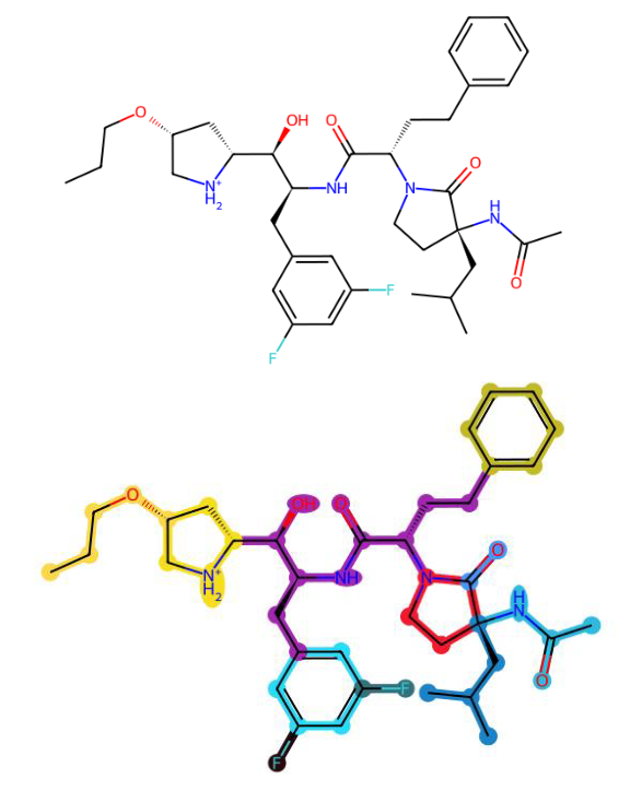
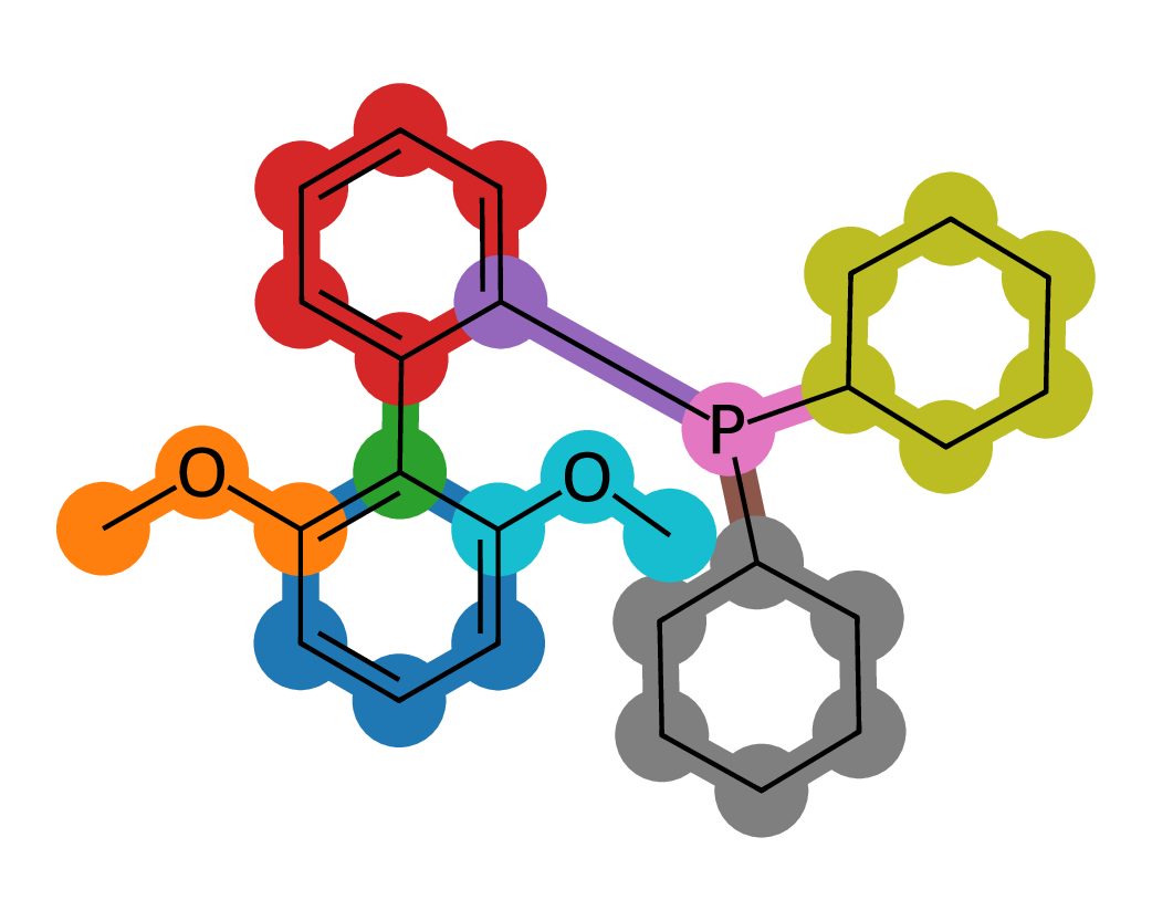
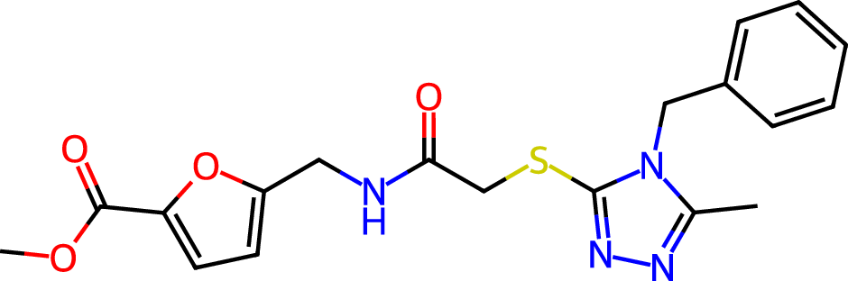
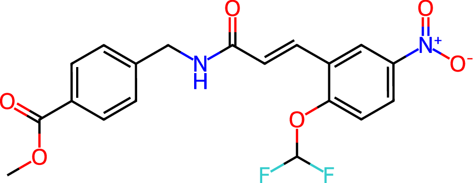
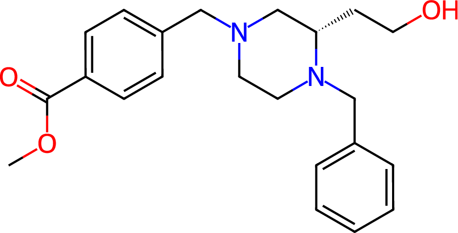
To enhance atomic representations with higher-order structural context, we construct a fragment-level graph from the input molecular graph $G$ using ring-path decomposition (Kong et al., 2022; Geng et al., 2023; Wollschläger et al., 2024) to identify key substructures such as aromatic rings and functional groups (Fig. 4). Each fragment is treated as a node in a new graph $G^{frag} = (V^{frag}, E^{frag})$ , where nodes correspond to fragments and edges are induced from the connectivity in $G$ , two fragments are connected if they share an atom or are directly bonded. In this work, we specifically follow the approach proposed in (Wollschläger et al., 2024), as it offers a good balance of simplicity and effectiveness for our use case.

We apply the same GAT formulation in Eq. (1) to the fragment graph to obtain fragment embeddings ${𝐡_{f}^{frag}}_{f \in V^{frag}}$ . Then for each atom $v$ that belongs to its fragment $f (v)$ , we fuse their atom-level representations $𝐡_{v}^{(L)}$ with ${𝐡_{f}^{frag}}$ by:

\tilde{𝐡}_{v}^{(L)} = 𝐡_{v}^{(L)} + F F N (𝐡_{f (v)}^{frag}),

(3)

where $F F N (\cdot)$ is a learnable feedforward network that projects fragment-level context into the same space as atom features. Finally, we define a fragment-enhanced graph level representation that is computed by applying a readout function $𝐡_{2 D} = 𝖱 𝖤 𝖠 𝖣 𝖮 𝖴 𝖳 ({\tilde{𝐡}_{v}^{(L)} ∣ v \in V}) = \sum_{v \in V} \tilde{𝐡}_{v}^{(L)} .$ Intuitively, the dual-level encoding combining local atomic features and global fragment-level context as Eq.(3) allows the model to reason over both fine-grained and coarse-grained structures, enhancing the expressivity of the molecular representation.

3.4 Learning Graph Transformer for 3D Molecule Aggregations

A molecular conformer is represented as a set $S = {𝐫_{i}, Z_{i}}_{i = 1}^{N}$ , where $N$ denotes the number of atoms, $𝐫_{i} \in ℝ^{3}$ corresponds to the 3D Cartesian coordinates of atom $i$ , and $Z_{i} \in ℕ$ indicates its atomic number.

3.4.1 3D conformer feature representation.

For each conformer $S$ , we can define its graph $𝒢_{S}$ and compute its 3D feature embedding by using the geometric MPNN SchNet (Schütt et al., 2017), though other $E (3)$ -invariant neural architectures can be readily substituted without modification (Table 3). We represent the matrix of atom-level features from the final message-passing layer $L$ of SchNet as $𝐇$ , where each column $𝐇 [v]$ corresponds to the feature vector $𝐡^{(L)}_{3 d, v}$ of atom $v$ . We then compute the vector representation of a conformer $S$ as $𝐡_{3 d, S} = \sum_{v \in V} (𝐖_{3 d}) 𝐡_{3 d, v}^{(L)} + 𝐛_{3 d} \in ℝ^{d}$ with $𝐖_{3 d}$ and $𝐛_{3 d}$ are learnable vectors. Given a set of $K$ conformers ${𝕊_{k}}_{k = 1}^{K}$ , we define $𝐇_{3 d} [k] = 𝐡_{3 D, 𝕊_{k}}$ as the feature embedding of the $k$ -th conformer. The matrix $𝐇_{3 d} \in ℝ^{K \times d}$ thus summarizes the feature representations of all conformers in the set.

3.4.2 Fragment-aware Graph Transformer.

Given the atom-wise feature matrix $𝐇$ for each conformer $S$ , we aim to learn structure-encoded latent representations using Graph Transformer architectures (Ying et al., 2021; Kreuzer et al., 2021; Luo et al., 2024). We adopt the architecture from Ying et al. (2021) due to its strong expressiveness on small molecular graphs, and further extend its attention mechanism with fragment sub-structures (Fig .4). It is important to note that our framework is flexible and can incorporate alternative transformer-based models.

In particular, we compose $N$ transformer layers (Vaswani et al., 2017), each consisting of a self-attention mechanism followed by a position-wise feed-forward network. Given $𝐇 = [𝐡_{1}^{⊤}, \dots, 𝐡_{n}^{⊤}]^{⊤} \in ℝ^{n \times d}$ computed in Section 3.4.1 by a 3D-MPNN, where $𝐡_{i} = 𝐡^{(L)}_{3 d, v_{i}} \in ℝ^{1 \times d}$ is the vector embedding of an atom $v_{i}$ with $d$ dimensions. We compute self-attention, by linearly projecting $𝐇$ into query ( $𝐐$ ), key ( $𝐊$ ), and value ( $𝐕$ ) matrices using learned weights $𝐖_{Q}, 𝐖_{K}, 𝐖_{V} \in ℝ^{d \times d}$ :

𝐐 = 𝐇 W_{Q}, 𝐊 = 𝐇 W_{K}, 𝐕 = 𝐇 W_{V}, \tilde{𝐀} = 𝐐 𝐊^{⊤} / \sqrt{d}, Attention (𝐇) = softmax (\tilde{𝐀}) 𝐕 .

(4)

Here, $\tilde{𝐀}$ denotes the attention score matrix representing pairwise similarities between tokens. For clarity, we present the single-head version; extending to multi-head attention is straightforward. Bias terms are omitted for brevity.

While the attention in Eq. (4) operates only on feature nodes, leveraging the structural information of the 3D conformer graph is essential. Following Ying et al. (2021), we incorporate (i) centrality encoding, which measures the importance of a node in the graph via its degree, and (ii) spatial encoding, which captures the spatial relation between two nodes $v_{i}$ and $v_{j}$ in $𝒢_{S}$ using the shortest path distance (SPD) (Cormen et al., 2022; Balaban, 1985), augmented with a learnable weight assigned to each edge along the SPD. Specifically, we incorporate (i) by:

𝐡_{i} = 𝐡_{i} + z^{-}_{deg^{-} (v_{i})} + z^{+}_{deg^{+} (v_{i})},

(5)

where $z^{-}, z^{+} \in ℝ^{d}$ are learnable embedding vectors specified by the indegree $deg^{-} (v_{i})$ and outdegree $deg^{+} (v_{i})$ of atom $v_{i}$ respectively. Here $z^{-}_{deg^{-} (v_{i})}$ is implemented as a lookup table of learnable embeddings indexed by shortest-path distance (i.e., degree) from node $v_{i}$ to others in the graph. The shortest-path distance (SPD) matrix is first computed, and these distances are used to retrieve the corresponding embeddings, which are then integrated into the attention mechanism to inject topology-aware structural bias. Assume $\tilde{𝐀}_{i j}$ as the $(i, j)$ -element of the Query-Key product matrix $\tilde{𝐀}$ , the condition (ii) extends $\tilde{𝐀}_{i j}$ as:

\tilde{𝐀}_{i j} = (𝐡_{𝐢} 𝐖_{Q}) (𝐡_{j} 𝐖_{K})^{T} / \sqrt{d} + s_{ϕ (v_{i}, v_{j})} + c_{i j},

(6)

where $s_{ϕ (v_{i}, v_{j})}$ is a learnable scalar indexed by the SPD distance $ϕ (v_{i}, v_{j})$ and shared across layers; $c_{i j} = 𝔼 (x_{e_{n}} (w^{E} n)^{T})$ , with $x e_{n}$ the feature of edge $e_{n}$ in $SPD_{i j}$ , $w_{n}^{E} \in ℝ^{d_{E}}$ its weight embedding, and $d_{E}$ the dimensionality of edge features, computed as the difference between the feature embeddings of its incident nodes.

While the spatial encoding in Eq.(6) is implicated by the SPD, we argue that this might inadequately capture chemically meaningful substructures (ablation in Tab. 3). This motivates us to extend attention scores in Eq. (6) using values derived from (iii) fragment-level node features computed on 2D topology graph in Eq. (3), directly guiding attention toward structurally and functionally relevant regions such as rings, functional groups, or scaffolds. To this end, we compute an adjacency-like matrix $𝐀 (G)$ using cosine distance over the final node embeddings $\tilde{𝐡}_{v}^{(L)}$ . Specifically, for each pair of atoms $(v_{i}, v_{j})$ in the 2D molecular graph, we define

𝐀 (G)_{i j} = 1 - \frac{⟨ \tilde{𝐡}_{i}^{(L)}, \tilde{𝐡}_{j}^{(L)} ⟩}{| \tilde{𝐡}_{i}^{(L)} |_{2} \cdot | \tilde{𝐡}_{j}^{(L)} |_{2}},

(7)

which quantifies their directional dissimilarity in the embedding space. Finally, we compute the attention score as:

\tilde{𝐀}_{i j} = (𝐡_{𝐢} 𝐖_{Q}) (𝐡_{j} 𝐖_{K})^{T} / \sqrt{d} + s_{ϕ (v_{i}, v_{j})} + c_{i j} + 𝐀 (G)_{i j} .

(8)

3.4.3 Learning to Approximate FGW distance.

We denote $𝒯_{θ} (.)$ as the graph transformer model whose attention operation is Eq.(8), our goal is to train $𝒯_{θ} (\cdot)$ to map the feature representation of each conformer $S$ into a latent space where the $L_{2}$ distance between any pair $S_{i}$ , $S_{j}$ approximates their FGW distance - an effective, yet computationally expensive, geometry-aware metric (Ma et al., 2023; Nguyen et al., 2024a). To this end, given a set of $Ω = {S_{i}}_{i = 1}^{K}$ of $K$ generated conformers, we sample $B$ conformers from $Ω$ , then compute their encoding features by $𝒯_{θ} (𝐇_{i})$ for each $S_{i} \in B$ . These outputs are compared with their pair-wise FGW distance to optimize the loss:

ℒ_{e n c} = \sum_{i j} | | | 𝒯_{θ} (𝐇_{i}) - 𝒯_{θ} (𝐇_{j}) | |_{2}^{2} - FGW_{p, α} (𝒢 (S_{i}), 𝒢 (S_{j})) | .

(9)

By minimizing the loss $ℒ_{enc}$ , we update the parameters of the transformation module $𝒯_{θ} (\cdot)$ using gradient descent: $θ \leftarrow θ - ϵ \nabla ℒ_{enc} .$ Once trained, we freeze $𝒯_{θ}$ and incorporate it back into the framework to compute a geometry-aware representation across $K$ conformers ${𝕊_{k}}_{k = 1}^{K}$ as follows: $\bar{𝐇} = 𝔼 ({𝒯_{θ} (𝐇_{i})}_{i = 1}^{K}),$ where $\bar{𝐇}$ denotes the aggregated structural embedding. However, the 3D conformer feature distribution, extracted by 3D-MPNN, used to train $ℒ_{enc}$ (Eq. 9) may experience a domain shift when co-trained with other components in the full framework (Sec. 3.4) due to the continuous updating of 3D-MPNN. To address this, we design adapter layers as simple FFN layers to transform the input features in Eq. (9), aligning them to the seen distribution during training $𝒯_{θ}$ .

3.4.4 Invariant Aggregation of 2D and 3D Representation.

We integrate representations from the 2D molecular graph and multiple 3D conformers using both average pooling and a GraphTransformer-based aggregation. The transformer captures rich spatial interactions while ensuring permutation invariance across conformers and E(3) equivariance, preserving robustness to 3D transformations. Given $K$ conformers, using $\bar{𝐇}$ as the GraphTransformer (GT)-aggregated atom features. We compute the global GT representation as: $𝐡_{G T} = \sum_{v \in V} (𝐖_{G T} \cdot \bar{𝐡}_{v} + 𝐛_{G T}),$ where $\bar{𝐡}_{v} = \bar{𝐇} [v]$ and $𝐖_{G T}, 𝐛_{G T}$ are learnable parameters. We then define $𝐇_{2 D}$ and $𝐇_{G T}$ be the matrices whose columns are, respectively, $K$ copies of the 2D feature $𝐡_{2 D}$ (Sec.3.3) and $𝐡_{G T}$ representations from previous section. We fuse those representations with the 3D conformer features $𝐇_{3 D}$ to produce the final atom-wise embedding: $𝐇_{c o m b} = \tilde{𝐖}_{2 D} 𝐇_{2 D} + \tilde{𝐖}_{3 D} 𝐇_{3 D} + \tilde{𝐖}_{G T} 𝐇_{G T},$ where each $\tilde{𝐖}_{i}, i \in {2 D, 3 D, G T}$ are trainable projection matrix. The combined embedding $𝐇_{c o m b}$ is fed into a final FFN layer to predict the target property (Sec.J Appendix).

4 Theoretical Bounds for Embedding Non-Euclidean FGW

Learning a Transformer $𝒯_{θ} (.)$ to predict the FGW problem is closely related to multidimensional scaling (MDS) (Torgerson, 1952). Building on recent advances (Haviv et al., 2024; Sonthalia et al., 2021), we extend MDS theory to derive bounds on the error of embedding non-Euclidean distances, specifically Wasserstein and FGW, into a Euclidean space suitable for graph transformer integration. While computing FGW barycenters is costly, our embedding enables efficient approximation via averaging and decoding in latent space. Prior work (Haviv et al., 2024) validated this approach for Wasserstein distances; we generalize it to FGW and provide theoretical justification, offering a scalable path for structure-aware graph alignment.

Cumulative Stress Optimization Problem via Pairwise FGW Distance Matrix. We define the pairwise FGW distance matrix $𝑫$ for a set of $K$ distributions as $D_{i j} : = FGW_{p, α} (𝒢 (S_{i}), 𝒢 (S_{j}))$ for all $i, j \in [K]$ , following Section 3.4. The empirical FGW barycenter is given by $\bar{𝒢}_{K} \in a r g m i n_{𝒢 \in 𝒫_{p} (𝛀)} \frac{1}{K} \sum_{i = 1}^{K} FGW_{p, α}^{p} (𝒢, 𝒢 (S_{i}))$ , where $𝒫_{p} (𝛀)$ denotes the space of attributed graphs with finite $p$ -th order FGW distance.

To approximate this barycenter in embedding space, we require $∥ \bar{𝒆}_{K} - 𝒆_{j} ∥_{2}^{2} \approx FGW_{p, α} (\bar{𝒢}_{K}, 𝒢 (S_{j})) : = \bar{D}_{K, j}$ for all $j \in [K]$ , where $\bar{𝒆}_{K} = \frac{1}{K} \sum_{i = 1}^{K} 𝒆_{i}$ is the mean embedding and $𝒆_{i} : = 𝒯_{θ} (𝐇_{i})$ is the learned representation. To assess how well the embeddings ${𝒆_{i}}_{i = 1}^{K} \subset ℝ^{d}$ preserve both pairwise FGW distances and barycenter structure, we define the cumulative stress: $𝒮 = \min_{𝒆_{i} \in ℝ^{d}} \sum_{i, j \in [K]} (∥ 𝒆_{i} - 𝒆_{j} ∥_{2}^{2} - D_{i j})^{2} + \sum_{j \in [K]} (∥ \bar{𝒆}_{K} - 𝒆_{j} ∥_{2}^{2} - \bar{D}_{K, j})^{2}$ . This objective encourages faithful reconstruction of both the distance structure and the barycenter alignment in the learned embedding space, as formalized in Theorem 1, which is proved in Appendix I.

Theorem 1.

Let $𝐃$ denote the pairwise $FGW_{p, α}$ distance matrix, and let ${λ_{i}, 𝐯_{i}}_{i = 1}^{K}$ represent the eigendecomposition of the associated criterion matrix $𝐅 = - 𝐂 𝐃 𝐂$ , where $𝐂 = 𝐈_{K} - \frac{1}{K} 𝟏_{K} 𝟏_{K}^{⊤}$ is the centering matrix. The optimal stress value, denoted by $𝒮^{*}$ , is bounded as follows: $ℒ \leq 𝒮^{*} \leq 𝒰$ , where $ℒ : = \sum_{i : λ_{i} < 0} λ_{i}^{2}$ , $𝒰 : = \sum_{i j} (Δ g_{i} + Δ g_{j})^{2} + ℒ + 𝒞$ , $Δ g_{i} = \frac{1}{2} \sum_{j : λ_{j} < 0} λ_{j} \cdot 𝐯_{i j}^{2}$ . Here, $𝐯_{i j}$ denotes the $j$ -th component of the $i$ -th eigenvector $𝐯_{n}$ of $𝐅$ , and $𝒞$ quantifies the approximation error between the empirical barycenter in the Euclidean embedding space and the one in the original space of undirected attributed graphs.

5 Experiments

5.1 Implementation Details

General pipeline. Our training consists of three stages. Stage 1: We train the 2D and 3D MPNNs independently for 150 epochs and the learning rate of $1 e^{- 3}$ to extract features from 2D molecular graphs and 3D conformers, used to predict molecular properties by regression loss. These extracted features also serve as a dataset to supervise the training of Graph Transformer for approximating the FGW distance. Stage 2: The Graph Transformer is trained separately to approximate the computationally expensive FGW distance between pairs of conformers, using the learned representations from Stage 1. We use the architecture of Graphormer (Ying et al., 2021), with 12 attention layers, 8 heads, and a hidden size of 64 (372k parameters). It is trained for 1000 epochs with a learning rate of $1 e^{- 5}$ . Stage 3: We train the full model end-to-end with 2D/3D MPNNs and the Graph Transformer (300 epochs, learning rate $5 e^{- 4}$ ). We further discuss this training scheme in Section G of the Appendix. To mitigate feature shift during finetuning, MLP-based adaptors map 3D conformers into 64-d refined embeddings, applied to both 2D and 3D features before the Graph Transformer.

5.2 Approximation of FGW Distance via Graph Transformer

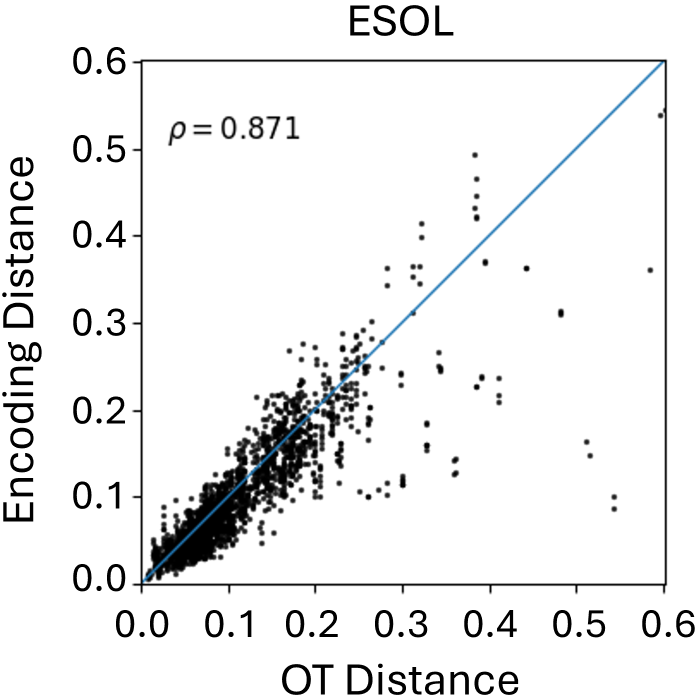
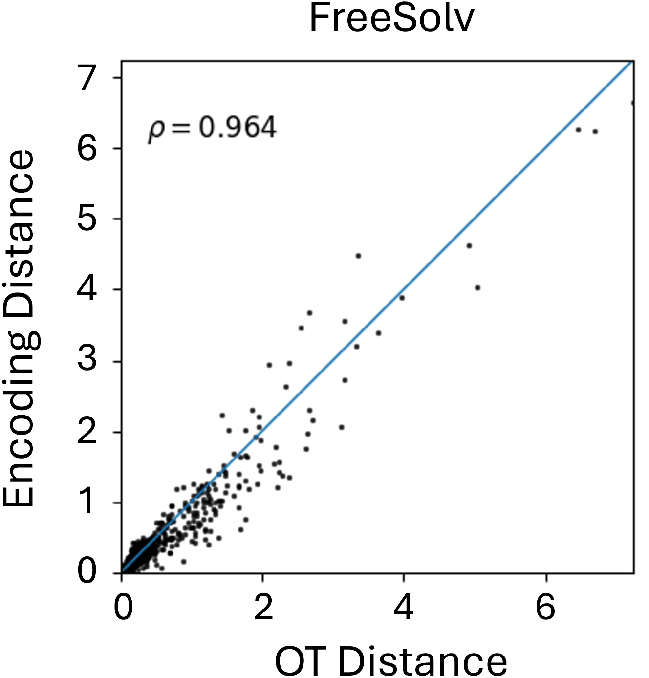
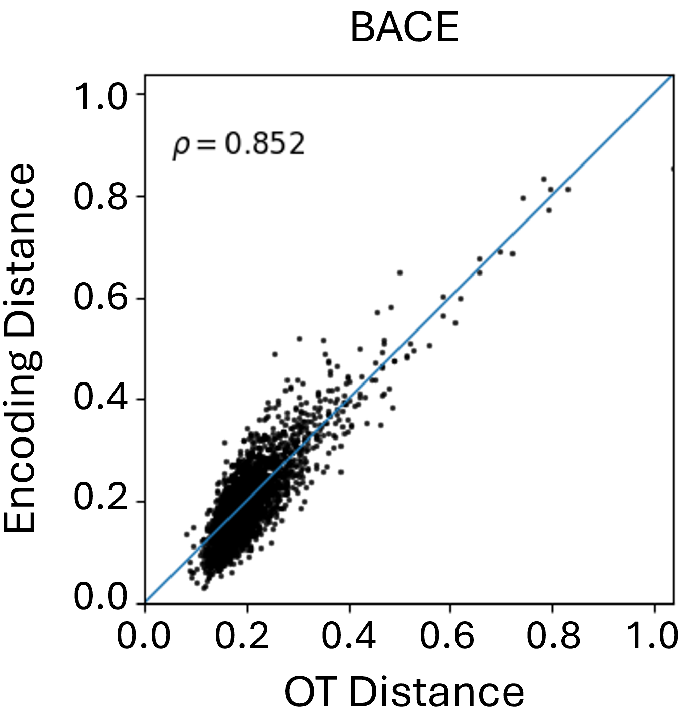
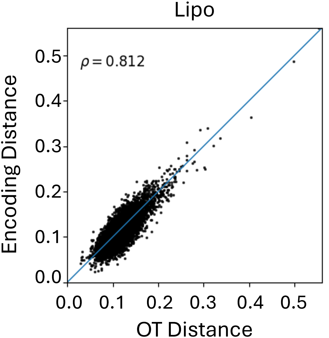
Beyond theoretical estimation, we empirically evaluate how well the Graph Transformer approximates FGW distances between conformers in Euclidean space. As shown in Figure 2, results on the MoleculeNet benchmarks reveal a strong correlation between learned embeddings and true FGW distances, validating the transformer’s effectiveness in simulating costly FGW computations. While correlation varies slightly across datasets, the results consistently highlight the model’s reliability as a fast FGW surrogate, especially as the number of conformers in the aggregation increases.

5.3 Scaling Fragment Geometry-Aware Aggregation

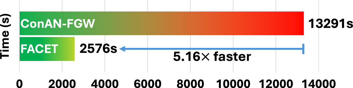
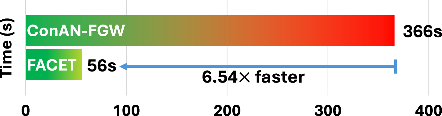
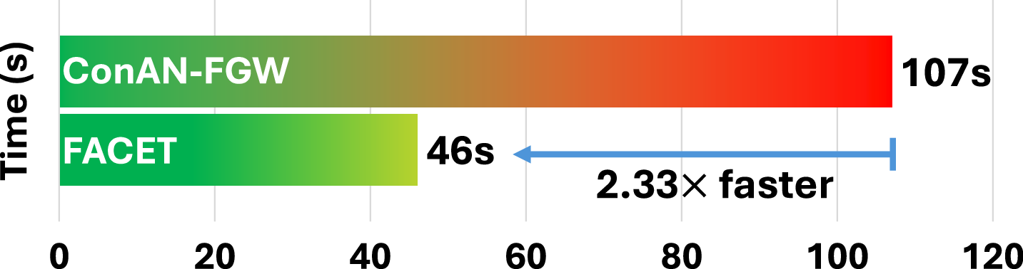
To validate the scalability of FACET model, based on a Graph Transformer for structure-aware aggregation, we compare it against Conan-FGW (Nguyen et al., 2024a), a method computing FGW distances on-the-fly during training and inference. We evaluate two key aspects: (i) inference-time efficiency with varying numbers of conformers, and (ii) average training time per epoch at different dataset scales. For inference, we measure the time required to generate output embeddings from $K$ conformers ( $K \in 5, 10, 15, 20$ ) using a single GPU. Experiments are conducted on FreeSolv and BACE, which differ in node/edge distributions, to assess performance across molecular graph complexities.

In the second setting, we compare the average per-epoch training time of FACET and Conan-FGW on two datasets of different scales: Kraken (1,086 molecules) and Drugs-75k (52,569 molecules). As summarized in Figures 7 (appendix) and 3, FACET exhibits linear scaling with the number of conformers and achieves 5–6× faster runtime on average than Conan-FGW. This efficiency is critical for scaling to large datasets and longer training schedules - for e.g, training Conan-FGW on Drugs-75k for 300 epochs requires 1,107.58 GPU hours, while FACET only takes 214 hours. This can be further reduced to 26.75 hours with 8 GPUs, compared to 138 hours for Conan-FGW under the same hardware setup. We present in Section D more analysis on this scaling factor.

Table 1: Number of samples for each split on molecular property prediction, classification tasks, and reaction prediction for MoleculeNet and the MARCEL benchmark.

Model	Lipo	ESOL	FreeSolv	BACE	Drugs-75k	Kraken
Train	2940	789	449	1059	52569	1086
Valid.	420	112	64	151	7509	155
Test	2940	227	129	303	15021	311
Total	4200	1128	642	1513	75099	1552

Table 2: FACET ablation study.

Settings	FACET	w/o Frag.	w/o Frag. in Trans.	w/o Adap.
ESOL	0.516	0.531	0.525	0.546
FreeSolv	0.967	1.072	0.973	1.085

Table 3: FACET results on SchNet and VisNet.

Model	Lipo	ESOL	FreeSolv	BACE
ConAN (VisNet)	$0.55 \pm 0.45$	$1.03 \pm 0.12$	$0.69 \pm 0.032$	$0.61 \pm 0.15$
ConAN-FGW	$0.50 \pm 0.008$	$0.55 \pm 0.05$	$0.64 \pm 0.02$	$0.47 \pm 0.01$
FACET	0.48 $\pm$ 0.01	0.53 $\pm$ 0.05	0.61 $\pm$ 0.02	0.47 $\pm$ 0.01
ConAN (SchNet)	$0.56 \pm 0.013$	$0.57 \pm 0.019$	$1.50 \pm 0.16$	$0.64 \pm 0.051$
ConAN-FGW	$0.42 \pm 0.02$	$0.53 \pm 0.02$	$1.07 \pm 0.08$	$0.55 \pm 0.02$
FACET	0.42 $\pm$ 0.01	0.52 $\pm$ 0.04	0.97 $\pm 0.08$	0.50 $\pm$ 0.03

5.4 State-of-the-Art Performance Comparison on Molecular Tasks

Datasets. We evaluate molecular property regression on the MoleculeNet (Wu et al., 2018) and MARCEL (Zhu et al., 2024a) benchmarks. MoleculeNet includes four datasets, ESOL, BACE, Lipo, and FreeSolv, with targets covering solubility, inhibitory concentration (pIC₅₀), lipophilicity, and hydration free energy. MARCEL consists of Drugs-75K and Kraken, where the goal is to predict the Boltzmann-averaged property $⟨ y ⟩_{k_{ℬ}}$ from sampled conformers. Drugs-75K uses quantum descriptors (IP, EA, $χ$ ), while Kraken focuses on Sterimol features (B₅, L, and their buried forms). The Boltzmann average is computed as a weighted sum over conformer-specific values $y_{i}$ with probabilities $p_{i}$ . All datasets follow the original random split settings, using the provided sampled conformers.

Baselines. For the MoleculeNet benchmark (Wu et al., 2018), we compare FACET with a wide range of baselines, including (i) 2D supervised methods (e.g., GAT (Veličković et al., 2018), D-MPNN (Yang et al., 2019a), AttentiveFP (Xiong et al., 2019)), (ii) pre-training approaches (e.g., PretrainGNN (Hu et al., 2020b), GROVER (Rong et al., 2020), ChemBERTa-2* (Ahmad et al., 2022), ChemRL-GEM (Fang et al., 2022), MolFormer (Ross et al., 2022)), (iii) 3D-conformers based models (ConfNet (Liu et al., 2021), UniMol (Zhou et al., 2023), SchNet (Schütt et al., 2017), ChemProp3D (Axelrod & Gómez-Bombarelli, 2023),ConAN-FGW (Nguyen et al., 2024b)). Training follows the setup in ConAN-FGW (Nguyen et al., 2024b).

For the MARCEL benchmark (Zhu et al., 2024a), we compare FACET against 2D models (e.g., GIN (Xu et al., 2019), GIN+VN (Hu et al., 2020a), ChemProp (Yang et al., 2019b), GraphGPS (Rampášek et al., 2022)), 3D models (e.g., SchNet (Schütt et al., 2017), DimeNet++ (Klicpera et al., 2020), GemNet (Gasteiger et al., 2021), PaiNN (Schütt et al., 2021), ClofNet (Du et al., 2022), LEFTNet (Du et al., 2023)), and ensemble strategies such as DeepSets-based ensemble (Zaheer et al., 2017), self-attention (Vaswani et al., 2017), etc. All methods are evaluated under the same settings as described in the MARCEL benchmark.

5.4.1 Results

Table 5: Comparison of molecular property regression performance on the MARCEL benchmark (MAE

↓

). The results of competing methods are adapted from Zhu et al. (2024a).

Category	Model	Drugs-75K			Kraken
	Model	IP	EA	$χ$	B₅	L	BurB₅	BurL
2D models	GIN	0.4354	0.4169	0.2260	0.3128	0.4003	0.1719	0.1200
	GIN+VN	0.4361	0.4169	0.2267	0.3567	0.4344	0.2422	0.1741
	ChemProp	0.4595	0.4417	0.2441	0.4850	0.5452	0.3002	0.1948
	GraphGPS	0.4351	0.4085	0.2212	0.3450	0.4363	0.2066	0.1500
3D models	SchNet	0.4394	0.4207	0.2243	0.3293	0.5458	0.2295	0.1861
	DimeNet++	0.4441	0.4233	0.2436	0.3510	0.4174	0.2097	0.1526
	GemNet	0.4069	0.3922	0.1970	0.2789	0.3754	0.1782	0.1635
	PaiNN	0.4505	0.4495	0.2324	0.3443	0.4471	0.2395	0.1673
	ClofNet	0.4393	0.4251	0.2378	0.4873	0.6417	0.2884	0.2529
	LEFTNet	0.4174	0.3964	0.2083	0.3072	0.4493	0.2176	0.1486
Ensemble Strategy with DeepSets	SchNet	0.4452	0.4232	0.2243	0.2704	0.4322	0.2024	0.1443
	DimeNet++	0.4126	0.3944	0.2267	0.2630	0.3468	0.1783	0.1185
	GemNet	0.4066	0.3910	0.2027	0.2313	0.3386	0.1589	0.0947
	PaiNN	0.4466	0.4269	0.2294	0.2225	0.3619	0.1693	0.1324
	ClofNet	0.4280	0.4033	0.2199	0.3228	0.4485	0.2178	0.1548
	LEFTNet	0.4149	0.3953	0.2069	0.2644	0.3643	0.2017	0.1386
FACET	SchNet	0.4235	0.3971	0.2155	0.2508	0.3982	0.1803	0.1245
FACET	GemNet	0.3891	0.3852	0.1970	0.2225	0.3402	0.1503	0.0952

MoleculeNet. As shown in Table 4, FACET achieves state-of-the-art performance on three molecular property regression tasks (ESOL, FreeSolv, BACE), with the lowest MSEs: $0.516 \pm 0.044$ , $0.967 \pm 0.082$ , and $0.495 \pm 0.115$ , respectively. Its consistent gains over CONAN-FGW indicate that, beyond geometry-aware aggregation, FACET’s use of fragment substructures (Figure 4) enhances attention to localized chemical contexts. This demonstrates the advantage of combining 3D spatial information with chemically meaningful substructures for molecular property prediction.

MARCEL. In Table 5, we evaluate FACET on two backbones, SchNet and GemNet. FACET consistently boosts both, confirming the benefits of structure-aware aggregation and fragment-level hierarchy. Unlike CONAN-FGW, which struggles to scale on the large MARCEL benchmark, FACET remains efficient and achieves near-SOTA performance across all targets, demonstrating robust effectiveness in diverse molecular property prediction tasks.

5.5 Ablation study

In this section, we analyze the key components of FACET through ablation studies. Specifically, we evaluate the impact of: (i) removing fragment structures from both the 2D MPNN and the self-attention mechanism in the graph transformer (w/o Frag); (ii) using fragments only in the 2D MPNN but not in the graph transformer (w/o Frag in Trans.); and (iii) omitting the trainable adaptor (w/o Adap.) that aligns 3D conformer features with the graph transformer, which can lead to performance degradation due to domain shift during training. As shown in Table 3, the absence of (i) significantly reduces performance, making FACET comparable to CONAN-FGW but with better scalability. Incorporating fragments into both components (ii) provides further gains, while (iii) proves essential for mitigating the domain shift introduced by changes in the 3D MPNN during training.

6 Conclusion

We present FACET, a scalable method that integrates 3D conformer features with fragment-level 2D graph information. Using an FGW-guided trainable attention mechanism, FACET dynamically fuses 2D and 3D representations, outperforming FGW-based baselines across all MoleculeNet tasks. It also scales to 75,000 molecules and large conformer ensembles in the MARCEL benchmark, achieving state-of-the-art results in property and reaction prediction with efficient runtimes. A discussion of the current limitations of FACET is presented in Section H Appendix.

References

Ahmad et al. (2022) Walid Ahmad, Elana Simon, Seyone Chithrananda, Gabriel Grand, and Bharath Ramsundar. Chemberta-2: Towards chemical foundation models, 2022. ↩ a b
Amos et al. (2023) Brandon Amos, Samuel Cohen, Giulia Luise, and Ievgen Redko. Meta optimal transport. International Conference on Machine Learning, 2023. ↩ a
Axelrod & Gomez-Bombarelli (2022) Simon Axelrod and Rafael Gomez-Bombarelli. Geom, energy-annotated molecular conformations for property prediction and molecular generation. Scientific Data, 9(1):185, 2022. ↩ a
Axelrod & Gomez-Bombarelli (2023) Simon Axelrod and Rafael Gomez-Bombarelli. Molecular machine learning with conformer ensembles. Machine Learning: Science and Technology, 4(3):035025, 2023. ↩ a
Axelrod & Gómez-Bombarelli (2023) Simon Axelrod and Rafael Gómez-Bombarelli. Molecular machine learning with conformer ensembles. Mach. Learn.: Sci. Technol., 4(3):035025, September 2023. ISSN 2632-2153. doi: 10.1088/2632-2153/acefa7. ↩ a
Bachmann et al. (2022) Fynn Bachmann, Philipp Hennig, and Dmitry Kobak. Wasserstein t-sne. In Joint European Conference on Machine Learning and Knowledge Discovery in Databases, pp. 104–120. Springer, 2022. ↩ a
Balaban (1985) Alexandru T Balaban. Applications of graph theory in chemistry. Journal of chemical information and computer sciences, 25(3):334–343, 1985. ↩ a
Batatia et al. (2022) Ilyes Batatia, David P Kovacs, Gregor Simm, Christoph Ortner, and Gabor Csanyi. Mace: Higher order equivariant message passing neural networks for fast and accurate force fields. In S. Koyejo, S. Mohamed, A. Agarwal, D. Belgrave, K. Cho, and A. Oh (eds.), Advances in Neural Information Processing Systems, volume 35, pp. 11423–11436. Curran Associates, Inc., 2022. ↩ a
Batatia et al. (2023) Ilyes Batatia, Philipp Benner, Yuan Chiang, Alin M. Elena, Dávid P. Kovács, Janosh Riebesell, Xavier R. Advincula, Mark Asta, William J. Baldwin, Noam Bernstein, Arghya Bhowmik, Samuel M. Blau, Vlad Cărare, James P. Darby, Sandip De, Flaviano Della Pia, Volker L. Deringer, Rokas Elijošius, Zakariya El-Machachi, Edvin Fako, Andrea C. Ferrari, Annalena Genreith-Schriever, Janine George, Rhys E. A. Goodall, Clare P. Grey, Shuang Han, Will Handley, Hendrik H. Heenen, Kersti Hermansson, Christian Holm, Jad Jaafar, Stephan Hofmann, Konstantin S. Jakob, Hyunwook Jung, Venkat Kapil, Aaron D. Kaplan, Nima Karimitari, Namu Kroupa, Jolla Kullgren, Matthew C. Kuner, Domantas Kuryla, Guoda Liepuoniute, Johannes T. Margraf, Ioan-Bogdan Magdău, Angelos Michaelides, J. Harry Moore, Aakash A. Naik, Samuel P. Niblett, Sam Walton Norwood, Niamh O’Neill, Christoph Ortner, Kristin A. Persson, Karsten Reuter, Andrew S. Rosen, Lars L. Schaaf, Christoph Schran, Eric Sivonxay, Tamás K. Stenczel, Viktor Svahn, Christopher Sutton, Cas van der Oord, Eszter Varga-Umbrich, Tejs Vegge, Martin Vondrák, Yangshuai Wang, William C. Witt, Fabian Zills, and Gábor Csányi. A foundation model for atomistic materials chemistry, 2023. ↩ a
Batzner et al. (2022) Simon Batzner, Albert Musaelian, Lixin Sun, Mario Geiger, Jonathan P. Mailoa, Mordechai Kornbluth, Nicola Molinari, Tess E. Smidt, and Boris Kozinsky. E(3)-equivariant graph neural networks for data-efficient and accurate interatomic potentials. Nat. Commun., 13(1):2453, May 2022. ISSN 2041-1723. ↩ a
Chan et al. (2024) Bill WGL Chan, Nicholas B Lynch, Wendy Tran, Jack M Joyce, G Paul Savage, Wim Meutermans, Andrew P Montgomery, and Michael Kassiou. Fragment-based drug discovery for disorders of the central nervous system: designing better drugs piece by piece. Frontiers in Chemistry, 12:1379518, 2024. ↩ a
Chithrananda et al. (2020) Seyone Chithrananda, Gabriel Grand, and Bharath Ramsundar. Chemberta: Large-scale self-supervised pretraining for molecular property prediction, 2020. ↩ a
Choudhary et al. (2022) Kamal Choudhary, Brian DeCost, Chi Chen, Anubhav Jain, Francesca Tavazza, Ryan Cohn, Cheol Woo Park, Alok Choudhary, Ankit Agrawal, Simon J. L. Billinge, Elizabeth Holm, Shyue Ping Ong, and Chris Wolverton. Recent advances and applications of deep learning methods in materials science. npj Comput. Mater., 8(1):59, Apr 2022. ISSN 2057-3960. ↩ a
Chung et al. (2019) Yongchul G Chung, Emmanuel Haldoupis, Benjamin J Bucior, Maciej Haranczyk, Seulchan Lee, Hongda Zhang, Konstantinos D Vogiatzis, Marija Milisavljevic, Sanliang Ling, Jeffrey S Camp, et al. Advances, updates, and analytics for the computation-ready, experimental metal–organic framework database: Core mof 2019. Journal of Chemical & Engineering Data, 64(12):5985–5998, 2019. ↩ a
Cormen et al. (2022) Thomas H Cormen, Charles E Leiserson, Ronald L Rivest, and Clifford Stein. Introduction to algorithms. MIT press, 2022. ↩ a
Courty et al. (2017) Nicolas Courty, Rémi Flamary, and Mélanie Ducoffe. Learning wasserstein embeddings. International Conference on Learning Representations (ICLR), 2017. ↩ a
Cuturi (2013) Marco Cuturi. Sinkhorn distances: Lightspeed computation of optimal transport. Advances in neural information processing systems, 26, 2013. ↩ a
Cuturi et al. (2020) Marco Cuturi, Olivier Teboul, Jonathan Niles-Weed, and Jean-Philippe Vert. Supervised quantile normalization for low rank matrix factorization. In International Conference on Machine Learning, pp. 2269–2279. PMLR, 2020. ↩ a
Degen et al. (2008) Jorg Degen, Christof Wegscheid-Gerlach, Andrea Zaliani, and Matthias Rarey. On the art of compiling and using’drug-like’chemical fragment spaces. ChemMedChem, 3(10):1503, 2008. ↩ a
Du et al. (2022) Weitao Du, He Zhang, Yuanqi Du, Qi Meng, Wei Chen, Nanning Zheng, Bin Shao, and Tie-Yan Liu. Se (3) equivariant graph neural networks with complete local frames. In International Conference on Machine Learning, pp. 5583–5608. PMLR, 2022. ↩ a
Du et al. (2023) Yuanqi Du, Limei Wang, Dieqiao Feng, Guifeng Wang, Shuiwang Ji, Carla P Gomes, Zhi-Ming Ma, et al. A new perspective on building efficient and expressive 3d equivariant graph neural networks. Advances in neural information processing systems, 36:66647–66674, 2023. ↩ a
Fang et al. (2021) Xiaomin Fang, Lihang Liu, Jieqiong Lei, Donglong He, Shanzhuo Zhang, Jingbo Zhou, Fan Wang, Hua Wu, and Haifeng Wang. Chemrl-gem: Geometry enhanced molecular representation learning for property prediction. Nature Machine Intelligence, 2021. doi: 10.48550/ARXIV.2106.06130. ↩ a
Fang et al. (2022) Xiaomin Fang, Lihang Liu, Jieqiong Lei, Donglong He, Shanzhuo Zhang, Jingbo Zhou, Fan Wang, Hua Wu, and Haifeng Wang. Geometry-enhanced molecular representation learning for property prediction. Nature Machine Intelligence, 4(2):127–134, 2022. ↩ a
Fedik et al. (2022) Nikita Fedik, Roman Zubatyuk, Maksim Kulichenko, Nicholas Lubbers, Justin S. Smith, Benjamin Nebgen, Richard Messerly, Ying Wai Li, Alexander I. Boldyrev, Kipton Barros, Olexandr Isayev, and Sergei Tretiak. Extending machine learning beyond interatomic potentials for predicting molecular properties. Nat. Rev. Chem., 6(9):653–672, Sep 2022. ISSN 2397-3358. doi: 10.1038/s41570-022-00416-3. ↩ a
Feydy et al. (2019) Jean Feydy, Thibault Séjourné, François-Xavier Vialard, Shun-ichi Amari, Alain Trouvé, and Gabriel Peyré. Interpolating between optimal transport and mmd using sinkhorn divergences. In The 22nd International Conference on aRtIfIcIaL InTeLlIgEnCe and Statistics, pp. 2681–2690. PMLR, 2019. ↩ a
Gasteiger et al. (2021) Johannes Gasteiger, Florian Becker, and Stephan Günnemann. Gemnet: Universal directional graph neural networks for molecules. Advances in Neural Information Processing Systems, 34:6790–6802, 2021. ↩ a
Genevay et al. (2018) Aude Genevay, Gabriel Peyré, and Marco Cuturi. Learning generative models with sinkhorn divergences. In International Conference on Artificial Intelligence and Statistics, pp. 1608–1617. PMLR, 2018. ↩ a
Geng et al. (2023) Zijie Geng, Shufang Xie, Yingce Xia, Lijun Wu, Tao Qin, Jie Wang, Yongdong Zhang, Feng Wu, and Tie-Yan Liu. De novo molecular generation via connection-aware motif mining. arXiv preprint arXiv:2302.01129, 2023. ↩ a b
Gilmer et al. (2017) Justin Gilmer, Samuel S. Schoenholz, Patrick F. Riley, Oriol Vinyals, and George E. Dahl. Neural message passing for quantum chemistry. In International Conference on Machine Learning, pp. 1263–1272, 2017. ↩ a
Gower (1985) J.C. Gower. Properties of Euclidean and non-Euclidean distance matrices. Linear Algebra and its Applications, 67:81–97, June 1985. ISSN 0024-3795. doi: 10.1016/0024-3795(85)90187-9. ↩ a
Haviv et al. (2024) Doron Haviv, Russell Zhang Kunes, Thomas Dougherty, Cassandra Burdziak, Tal Nawy, Anna Gilbert, and Dana Pe’Er. Wasserstein Wormhole: Scalable Optimal Transport Distance with Transformer. In Ruslan Salakhutdinov, Zico Kolter, Katherine Heller, Adrian Weller, Nuria Oliver, Jonathan Scarlett, and Felix Berkenkamp (eds.), Proceedings of the 41st International Conference on Machine Learning, volume 235 of Proceedings of Machine Learning Research, pp. 17697–17718. PMLR, July 2024. ↩ a b c
Hawkins (2017) Paul CD Hawkins. Conformation generation: the state of the art. Journal of chemical information and modeling, 57(8):1747–1756, 2017. ↩ a
Hetzel et al. (2023) Leon Hetzel, Johanna Sommer, Bastian Rieck, Fabian Theis, and Stephan Günnemann. MAGNet: Motif-agnostic generation of molecules from shapes. arXiv preprint arXiv:2305.19303, 2023. ↩ a
Higham (1988) Nicholas J. Higham. Computing a nearest symmetric positive semidefinite matrix. Linear Algebra and its Applications, 103:103–118, May 1988. ISSN 0024-3795. doi: 10.1016/0024-3795(88)90223-6. ↩ a
Hu et al. (2020a) Weihua Hu, Matthias Fey, Marinka Zitnik, Yuxiao Dong, Hongyu Ren, Bowen Liu, Michele Catasta, and Jure Leskovec. Open graph benchmark: Datasets for machine learning on graphs. Advances in neural information processing systems, 33:22118–22133, 2020a. ↩ a
Hu et al. (2020b) Weihua Hu, Bowen Liu, Joseph Gomes, Marinka Zitnik, Percy Liang, Vijay Pande, and Jure Leskovec. Strategies for pre-training graph neural networks. In International Conference on Learning Representations, 2020b. ↩ a
Klicpera et al. (2020) Johannes Klicpera, Janek Groß, Stephan Günnemann, et al. Directional message passing for molecular graphs. In International Conference on Learning Representations, pp. 1–13, 2020. ↩ a
Kong et al. (2022) Xiangzhe Kong, Wenbing Huang, Zhixing Tan, and Yang Liu. Molecule generation by principal subgraph mining and assembling. Advances in Neural Information Processing Systems, 35:2550–2563, 2022. ↩ a b
Kreuzer et al. (2021) Devin Kreuzer, Dominique Beaini, Will Hamilton, Vincent Létourneau, and Prudencio Tossou. Rethinking graph transformers with spectral attention. Advances in Neural Information Processing Systems, 34:21618–21629, 2021. ↩ a
Landrum (2016) G Landrum. Rdkit: open-source cheminformatics http://www.rdkit.org, 2016. ↩ a
Lee et al. (2024) Seul Lee, Seanie Lee, Kenji Kawaguchi, and Sung Ju Hwang. Drug discovery with dynamic goal-aware fragments. International Conference on Machine Learning, 2024. ↩ a
Liu et al. (2021) Meng Liu, Cong Fu, Xuan Zhang, Limei Wang, Yaochen Xie, Hao Yuan, Youzhi Luo, Zhao Xu, Shenglong Xu, and Shuiwang Ji. Fast quantum property prediction via deeper 2d and 3d graph networks. arXiv preprint arXiv:2106.08551, 2021. ↩ a
Liu et al. (2015) Zhihai Liu, Yan Li, Li Han, Jie Li, Jie Liu, Zhixiong Zhao, Wei Nie, Yuchen Liu, and Renxiao Wang. Pdb-wide collection of binding data: current status of the pdbbind database. Bioinformatics, 31(3):405–412, 2015. ↩ a
Luo et al. (2024) Yuankai Luo, Hongkang Li, Lei Shi, and Xiao-Ming Wu. Enhancing graph transformers with hierarchical distance structural encoding. Advances in Neural Information Processing Systems, 37:57150–57182, 2024. ↩ a
Ma et al. (2023) Xinyu Ma, Xu Chu, Yasha Wang, Yang Lin, Junfeng Zhao, Liantao Ma, and Wenwu Zhu. Fused gromov-wasserstein graph mixup for graph-level classifications. In Thirty-seventh Conference on Neural Information Processing Systems, 2023. ↩ a b c
Medrano Sandonas et al. (2024) Leonardo Medrano Sandonas, Dries Van Rompaey, Alessio Fallani, Mathias Hilfiker, David Hahn, Laura Perez-Benito, Jonas Verhoeven, Gary Tresadern, Joerg Kurt Wegner, Hugo Ceulemans, et al. Dataset for quantum-mechanical exploration of conformers and solvent effects in large drug-like molecules. Scientific Data, 11(1):742, 2024. ↩ a
Merlot et al. (2003) Cédric Merlot, Daniel Domine, Christophe Cleva, and Dennis J Church. Chemical substructures in drug discovery. Drug Discovery Today, 8(13):594–602, 2003. ↩ a
Morgan (1965) H. L. Morgan. The generation of a unique machine description for chemical structures-a technique developed at chemical abstracts service. Journal of Chemical Documentation, 5(2):107–113, May 1965. ISSN 1541-5732. doi: 10.1021/c160017a018. ↩ a
Nguyen et al. (2024a) Duy MH Nguyen, Nina Lukashina, Tai Nguyen, An T Le, TrungTin Nguyen, Nhat Ho, Jan Peters, Daniel Sonntag, Viktor Zaverkin, and Mathias Niepert. Structure-aware e (3)-invariant molecular conformer aggregation networks. International Conference on Machine Learning, 2024a. ↩ a b c d
Nguyen et al. (2024b) Duy Minh Ho Nguyen, Nina Lukashina, Tai Nguyen, An Thai Le, Trungtin Nguyen, Nhat Ho, Jan Peters, Daniel Sonntag, Viktor Zaverkin, and Mathias Niepert. Structure-aware E(3)-invariant molecular conformer aggregation networks. In International Conference on Machine Learning, pp. 37736–37760. PMLR, 2024b. ↩ a b c d e f g
Otsuka et al. (2011) Shingo Otsuka, Isao Kuwajima, Junko Hosoya, Yibin Xu, and Masayoshi Yamazaki. Polyinfo: Polymer database for polymeric materials design. In 2011 International Conference on Emerging Intelligent Data and Web Technologies, pp. 22–29. IEEE, 2011. ↩ a
Perola & Charifson (2004) Emanuele Perola and Paul S Charifson. Conformational analysis of drug-like molecules bound to proteins: an extensive study of ligand reorganization upon binding. Journal of medicinal chemistry, 47(10):2499–2510, 2004. ↩ a
Peyré et al. (2016) Gabriel Peyré, Marco Cuturi, and Justin Solomon. Gromov-Wasserstein Averaging of Kernel and Distance Matrices. In Maria Florina Balcan and Kilian Q. Weinberger (eds.), Proceedings of The 33rd International Conference on Machine Learning, volume 48 of Proceedings of Machine Learning Research, pp. 2664–2672, New York, New York, USA, June 2016. PMLR. ↩ a
Peyré et al. (2019) Gabriel Peyré, Marco Cuturi, and others. Computational optimal transport: With applications to data science. Foundations and Trends in Machine Learning, 11(5-6):355–607, 2019. Publisher: Now Publishers, Inc. ↩ a
Rampášek et al. (2022) Ladislav Rampášek, Michael Galkin, Vijay Prakash Dwivedi, Anh Tuan Luu, Guy Wolf, and Dominique Beaini. Recipe for a general, powerful, scalable graph transformer. Advances in Neural Information Processing Systems, 35:14501–14515, 2022. ↩ a
Ramsundar et al. (2019) Bharath Ramsundar, Peter Eastman, Pat Walters, and Vijay Pande. Deep learning for the life sciences: applying deep learning to genomics, microscopy, drug discovery, and more. O’Reilly Media, 2019. ↩ a
Raza et al. (2022) Ali Raza, E Adrian Henle, and Xiaoli Fern. Non-equilibrium molecular geometries in graph neural networks. arXiv preprint arXiv:2203.04697, 2022. ↩ a
Rong et al. (2020) Yu Rong, Yatao Bian, Tingyang Xu, Weiyang Xie, Ying Wei, Wenbing Huang, and Junzhou Huang. Self-supervised graph transformer on large-scale molecular data. Advances in Neural Information Processing Systems, 33:12559–12571, 2020. ↩ a b c
Ross et al. (2022) Jerret Ross, Brian Belgodere, Vijil Chenthamarakshan, Inkit Padhi, Youssef Mroueh, and Payel Das. Large-scale chemical language representations capture molecular structure and properties. Nature Machine Intelligence, 4(12):1256–1264, 2022. ↩ a
Scarselli et al. (2008) Franco Scarselli, Marco Gori, Ah Chung Tsoi, Markus Hagenbuchner, and Gabriele Monfardini. The graph neural network model. IEEE transactions on neural networks, 20(1):61–80, 2008. ↩ a
Scetbon et al. (2021) Meyer Scetbon, Marco Cuturi, and Gabriel Peyré. Low-rank sinkhorn factorization. In International Conference on Machine Learning, pp. 9344–9354. PMLR, 2021. ↩ a
Schütt et al. (2017) Kristof Schütt, Pieter-Jan Kindermans, Huziel Enoc Sauceda Felix, Stefan Chmiela, Alexandre Tkatchenko, and Klaus-Robert Müller. Schnet: A continuous-filter convolutional neural network for modeling quantum interactions. In Advances in Neural Information Processing Systems 30: Annual Conference on Neural Information Processing Systems 2017, December 4-9, 2017, Long Beach, CA, USA, pp. 991–1001, 2017. ↩ a
Schütt et al. (2017) Kristof Schütt, Pieter-Jan Kindermans, Huziel Enoc Sauceda Felix, Stefan Chmiela, Alexandre Tkatchenko, and Klaus-Robert Müller. Schnet: A continuous-filter convolutional neural network for modeling quantum interactions. In I. Guyon, U. Von Luxburg, S. Bengio, H. Wallach, R. Fergus, S. Vishwanathan, and R. Garnett (eds.), Advances in Neural Information Processing Systems, volume 30. Curran Associates, Inc., 2017. ↩ a b c
Schütt et al. (2021) Kristof Schütt, Oliver Unke, and Michael Gastegger. Equivariant message passing for the prediction of tensorial properties and molecular spectra. In International Conference on Machine Learning, pp. 9377–9388. PMLR, 2021. ↩ a
Solomon et al. (2015) Justin Solomon, Fernando De Goes, Gabriel Peyré, Marco Cuturi, Adrian Butscher, Andy Nguyen, Tao Du, and Leonidas Guibas. Convolutional wasserstein distances: Efficient optimal transportation on geometric domains. ACM Transactions on Graphics (ToG), 34(4):1–11, 2015. ↩ a
Sommer et al. (2023) Johanna Sommer, Leon Hetzel, David Lüdke, Fabian Theis, and Stephan Günnemann. The power of motifs as inductive bias for learning molecular distributions. arXiv preprint arXiv:2306.17246, 2023. ↩ a
Sonthalia et al. (2021) Rishi Sonthalia, Greg Van Buskirk, Benjamin Raichel, and Anna Gilbert. How can classical multidimensional scaling go wrong? In M. Ranzato, A. Beygelzimer, Y. Dauphin, P. S. Liang, and J. Wortman Vaughan (eds.), Advances in Neural Information Processing Systems, volume 34, pp. 12304–12315. Curran Associates, Inc., 2021. ↩ a
Titouan et al. (2019) Vayer Titouan, Nicolas Courty, Romain Tavenard, Chapel Laetitia, and Rémi Flamary. Optimal Transport for structured data with application on graphs. In Kamalika Chaudhuri and Ruslan Salakhutdinov (eds.), Proceedings of the 36th International Conference on Machine Learning, volume 97 of Proceedings of Machine Learning Research, pp. 6275–6284. PMLR, June 2019. ↩ a
Titouan et al. (2020) Vayer Titouan, Laetitia Chapel, Remi Flamary, Romain Tavenard, and Nicolas Courty. Fused Gromov-Wasserstein Distance for Structured Objects. Algorithms, 13(9):212, August 2020. ISSN 1999-4893. doi: 10.3390/a13090212. ↩ a
Tong et al. (2021) Alexander Y Tong, Guillaume Huguet, Amine Natik, Kincaid MacDonald, Manik Kuchroo, Ronald Coifman, Guy Wolf, and Smita Krishnaswamy. Diffusion earth mover’s distance and distribution embeddings. In International Conference on Machine Learning, pp. 10336–10346. PMLR, 2021. ↩ a
Torgerson (1952) Warren S. Torgerson. Multidimensional Scaling: I. Theory and Method. Psychometrika, 17(4):401–419, 1952. ISSN 0033-3123. doi: 10.1007/BF02288916. Edition: 2025/01/01 Publisher: Cambridge University Press & Assessment. ↩ a
Varnek et al. (2005) Alexandre Varnek, Denis Fourches, Frank Hoonakker, and Vitaly P Solov’ev. Substructural fragments: an universal language to encode reactions, molecular and supramolecular structures. Journal of computer-aided molecular design, 19:693–703, 2005. ↩ a
Vaswani et al. (2017) Ashish Vaswani, Noam Shazeer, Niki Parmar, Jakob Uszkoreit, Llion Jones, Aidan N Gomez, Łukasz Kaiser, and Illia Polosukhin. Attention is all you need. Advances in neural information processing systems, 30, 2017. ↩ a b c
Veličković et al. (2017) Petar Veličković, Guillem Cucurull, Arantxa Casanova, Adriana Romero, Pietro Lio, and Yoshua Bengio. Graph attention networks. arXiv preprint arXiv:1710.10903, 2017. ↩ a
Veličković et al. (2018) Petar Veličković, Guillem Cucurull, Arantxa Casanova, Adriana Romero, Pietro Liò, and Yoshua Bengio. Graph attention networks. In International Conference on Learning Representations, 2018. ↩ a
Veličković et al. (2018) Petar Veličković, Guillem Cucurull, Arantxa Casanova, Adriana Romero, Pietro Liò, and Yoshua Bengio. Graph attention networks. In ICLR, 2018. ↩ a
Wang et al. (2025) Jiaxi Wang, Yaosen Min, Miao Li, and Ji Wu. Fragformer: A fragment-based representation learning framework for molecular property prediction. Transactions on Machine Learning Research, 2025. ↩ a
Wang et al. (2019) Sheng Wang, Yuzhi Guo, Yuhong Wang, Hongmao Sun, and Junzhou Huang. Smiles-bert: Large scale unsupervised pre-training for molecular property prediction. In Proceedings of the 10th ACM International Conference on Bioinformatics, Computational Biology and Health Informatics, BCB ’19, pp. 429–436, New York, NY, USA, 2019. Association for Computing Machinery. ISBN 9781450366663. doi: 10.1145/3307339.3342186. ↩ a
Wang et al. (2024) Zeyu Wang, Tianyi Jiang, Jinhuan Wang, and Qi Xuan. Multi-modal representation learning for molecular property prediction: Sequence, graph, geometry. arXiv preprint arXiv:2401.03369, 2024. ↩ a
Wen et al. (2024) Qianlong Wen, Mingxuan Ju, Zhongyu Ouyang, Chuxu Zhang, and Yanfang Ye. From coarse to fine: enable comprehensive graph self-supervised learning with multi-granular semantic ensemble. In Forty-first International Conference on Machine Learning, 2024. ↩ a
Wollschläger et al. (2024) Tom Wollschläger, Niklas Kemper, Leon Hetzel, Johanna Sommer, and Stephan Günnemann. Expressivity and generalization: Fragment-biases for molecular gnns. International Conference on Machine Learning, 2024. ↩ a b c d
Wu et al. (2018) Z. Wu, B. Ramsundar, E. N. Feinberg, J. Gomes, C. Geniesse, A. S. Pappu, K. Leswing, and V. Pande. MoleculeNet: A benchmark for molecular machine learning. Chemical Science, pp. 513–530, 2018. ↩ a b
Xiong et al. (2019) Zhaoping Xiong, Dingyan Wang, Xiaohong Liu, Feisheng Zhong, Xiaozhe Wan, Xutong Li, Zhaojun Li, Xiaomin Luo, Kaixian Chen, Hualiang Jiang, et al. Pushing the boundaries of molecular representation for drug discovery with the graph attention mechanism. Journal of medicinal chemistry, 63(16):8749–8760, 2019. ↩ a
Xu et al. (2018) Keyulu Xu, Chengtao Li, Yonglong Tian, Tomohiro Sonobe, Ken-ichi Kawarabayashi, and Stefanie Jegelka. Representation learning on graphs with jumping knowledge networks. In Jennifer Dy and Andreas Krause (eds.), Proceedings of the 35th International Conference on Machine Learning, volume 80 of Proceedings of Machine Learning Research, pp. 5453–5462. PMLR, 10–15 Jul 2018. ↩ a
Xu et al. (2019) Keyulu Xu, Weihua Hu, Jure Leskovec, and Stefanie Jegelka. How powerful are graph neural networks? International Conference on Learning Representations, 2019. ↩ a
Yang et al. (2019a) Kevin Yang, Kyle Swanson, Wengong Jin, Connor Coley, Philipp Eiden, Hua Gao, Angel Guzman-Perez, Timothy Hopper, Brian Kelley, Miriam Mathea, Andrew Palmer, Volker Settels, Tommi Jaakkola, Klavs Jensen, and Regina Barzilay. Analyzing learned molecular representations for property prediction. Journal of Chemical Information and Modeling, 59(8):3370–3388, July 2019a. ISSN 1549-960X. doi: 10.1021/acs.jcim.9b00237. ↩ a b
Yang et al. (2019b) Kevin Yang, Kyle Swanson, Wengong Jin, Connor Coley, Philipp Eiden, Hua Gao, Angel Guzman-Perez, Timothy Hopper, Brian Kelley, Miriam Mathea, et al. Analyzing learned molecular representations for property prediction. Journal of chemical information and modeling, 59(8):3370–3388, 2019b. ↩ a
Ying et al. (2021) Chengxuan Ying, Tianle Cai, Shengjie Luo, Shuxin Zheng, Guolin Ke, Di He, Yanming Shen, and Tie-Yan Liu. Do transformers really perform badly for graph representation? Advances in neural information processing systems, 34:28877–28888, 2021. ↩ a b c d e f
Zaheer et al. (2017) Manzil Zaheer, Satwik Kottur, Siamak Ravanbakhsh, Barnabas Poczos, Russ R Salakhutdinov, and Alexander J Smola. Deep sets. Advances in neural information processing systems, 30, 2017. ↩ a b
Zhang et al. (2021) Zaixi Zhang, Qi Liu, Hao Wang, Chengqiang Lu, and Chee-Kong Lee. Motif-based graph self-supervised learning for molecular property prediction. Advances in Neural Information Processing Systems, 34:15870–15882, 2021. ↩ a
Zhou et al. (2023) Gengmo Zhou, Zhifeng Gao, Qiankun Ding, Hang Zheng, Hongteng Xu, Zhewei Wei, Linfeng Zhang, and Guolin Ke. Uni-mol: A universal 3d molecular representation learning framework. In The Eleventh International Conference on Learning Representations, 2023. ↩ a b c
Zhu et al. (2024a) Y Zhu, J Hwang, K Adams, Z Liu, B Nan, B Stenfors, Y Du, J Chauhan, O Wiest, O Isayev, et al. Learning over molecular conformer ensembles: Datasets and benchmarks. In International Conference on Learning Representations, 2024a. ↩ a b c
Zhu et al. (2023) Yanqiao Zhu, Jeehyun Hwang, Keir Adams, Zhen Liu, Bozhao Nan, Brock Stenfors, Yuanqi Du, Jatin Chauhan, Olaf Wiest, Olexandr Isayev, Connor W. Coley, Yizhou Sun, and Wei Wang. Learning over molecular conformer ensembles: Datasets and benchmarks, 2023. ↩ a
Zhu et al. (2024b) Yanqiao Zhu, Jeehyun Hwang, Keir Adams, Zhen Liu, Bozhao Nan, Brock Stenfors, Yuanqi Du, Jatin Chauhan, Olaf Wiest, Olexandr Isayev, et al. Learning over molecular conformer ensembles: Datasets and benchmarks. International Conference on Learning Representations (ICLR), 2024b. ↩ a b

Appendix A Implementation Details

Our training pipeline includes three stages: In the first stage, we train only the 2D and 3D MPNNs to learn corresponding features from 2D molecular graph and 3D conformers. The features in this stage also serve as a dataset for approximating Graph Transformer to the FGW distance. In the next stage, the Graph Transformer is trained separately to simulate the costly computation of FGW distance between two conformers using learned features from stage 1. In the last stage, Graph Transformer is integrated in a single end-to-end training with 2D and 3D MPNNs. At this stage, only 2D and 3D MPNNs are trained. As a result of changing MPNNs during the last stage, a shift in the distribution of the Graph Transformer input might occur. We solve this problem by adding an adaptor layer using an MLP on both 3D and 2D features before feeding them to the GraphTransformer. For all experiments on the MoleculeNet and MARCEL benchmarks, we use the same number of conformers as specified in their original settings.

In all stages, we use Adam as our optimizer. We train our model on an 8 V100-GPUs cluster.

Stage 1. Learning 2D and 3D features.

For each molecule, we define by $𝐇_{2 d - 3 d} = \tilde{𝐖}_{2 D} 𝐇_{2 D} + \tilde{𝐖}_{3 D} 𝐇_{3 D}$ , we then train for 150 epochs and set the learning rate to $1 e^{- 3}$ . to optimize target property tasks $ℒ_{p r e d} = | | \hat{𝒚}_{2 d - 3 d} - \tilde{𝐲} | |_{2}^{2}$ where $\tilde{𝐲}$ be the ground-truth value and $\hat{𝒚}$ be our predicted value defined by:

\hat{𝒚}_{2 d - 3 d} = 𝐖^{𝒢} (\frac{1}{K} \sum_{k = 1}^{K} 𝐇_{2 d - 3 d} [k]) + 𝐛^{𝒢},

(10)

with $𝐖^{𝒢}$ and $𝐛^{𝒢}$ are learnable parameters and $K$ is number of conformers.

Stage 2. Training Graph Transformer to approximate FGW distance.

The Graph Transformer is trained separately in the second stage to approximate the FGW distance by Euclidean embedding space. For the Graph Transformer architecture, we employ the same setting as Graphormer from Ying et al. (2021). Specifically, a number of attention layers, a number of attention heads, and the hidden dimension of the transformer are set to 12, 8, and 64, respectively, which makes the total number of parameters of the Graph Transformer 372k. In our attention, we use the shortest-path distance (SPD) between a pair of nodes. Following practical implementation in Ying et al. (2021), we pre-compute SPD distance for each 3D molecule graph and load these values during training and inference. We set a learning rate of $1 e^{- 5}$ and train for 1000 epochs with the following loss function:

ℒ_{e n c} = \sum_{i j} [| | 𝒯_{θ} (𝐇_{i}) - 𝒯_{θ} (𝐇_{j}) | |_{2}^{2} - FGW_{p, α} (𝒢 (S_{i}), 𝒢 (S_{j}))] .

(11)

Stage 3. Training Fragment-aware Graph Transformer. In the final stage, we freeze the trained GraphTransformer $𝒯 θ (\cdot)$ and use it to compute aggregated features from 3D conformer embeddings generated by the 3D-MPNN. To accommodate potential distribution shifts, we add lightweight FFN adaptor layers on top of both the 2D- and 3D-MPNNs used in $𝒯 θ (\cdot)$ , while continuing to update the MPNNs during training. The full model is trained for 300 epochs with a reduced learning rate to optimize the training loss $ℒ_{p r e d} = | | \hat{𝒚} - \tilde{𝐲} | |_{2}^{2}$ where

\hat{𝒚} = 𝐖^{𝒢} (\frac{1}{K} \sum_{k = 1}^{K} 𝐇_{c o m b} [k]) + 𝐛^{𝒢} .

(12)

$𝐇_{c o m b}$ is final atom-wise embedding.

Appendix B Further Visualization Fragment Outputs

Fragment Generation Algorithms.

We use a structural fragmentation method based on RingPath algorithms (Kong et al., 2022; Geng et al., 2023; Wollschläger et al., 2024) that decompose a molecular graph $G = (V, E)$ , where $V$ denotes atoms and $E$ denotes covalent bonds, into a set of chemically interpretable fragments. The fragmentation process identifies a set of ring fragments $ℱ_{ring} \subseteq ℱ$ using RDKit’s cycle basis algorithm (SSSR), where each ring $f_{r} \in ℱ_{ring}$ is encoded by its atom indices and size class.

Next, all bonds not part of any ring are grouped into acyclic path fragments $ℱ_{path} \subseteq ℱ$ , where each $f_{p} \in ℱ_{path}$ is a linear chain of nodes, extracted via depth-first search under a degree constraint. Each fragment $f \in ℱ = ℱ_{ring} \cup ℱ_{path} \cup ℱ_{junction}$ is assigned a type $t (f) \in {0, 1, 2}$ (representing ring, path, or junction) and a type index $ϕ (f) \in {0, 1, \dots, K - 1}$ within a fixed vocabulary of size $K$ . Fragments whose sizes exceed a predefined threshold $k_{\max}$ are mapped to the final index of their category to preserve bounded dimensionality.

We define a fragment-atom incidence matrix $M \in {0, 1}^{| V | \times | ℱ |}$ , where $M_{v, f} = 1$ if atom $v \in V$ belongs to fragment $f$ . From this, we derive a fragment-level graph $G^{frag} = (V_{frag}, E_{frag})$ , where each node $f \in ℱ$ represents a molecular fragment and an edge $(f_{i}, f_{j}) \in E_{frag}$ is added if two fragments share at least one atom or are directly bonded.

Compared to traditional fragmentation algorithms like BRICS (Degen et al., 2008), BBB (Sommer et al., 2023), or MagNet (Hetzel et al., 2023), the RingPath algorithm offers a more topology-aware decomposition by explicitly capturing key structural motifs such as rings, paths, and linkers. While BRICS and BBB often generate chemically meaningful fragments based on retrosynthetic rules, they may overlook contextual connectivity critical for graph-based learning. In contrast, RingPath preserves the relational structure between fragments, aligning closely with how molecules are built and understood in topological space—making it particularly beneficial for tasks requiring structural interpretability and generalization in graph neural networks. The advantages of RingPath have also been empirically validated in recent studies, demonstrating improved performance across various molecular property prediction benchmarks.

Visualization of Typical Extracted Fragment Graphs.

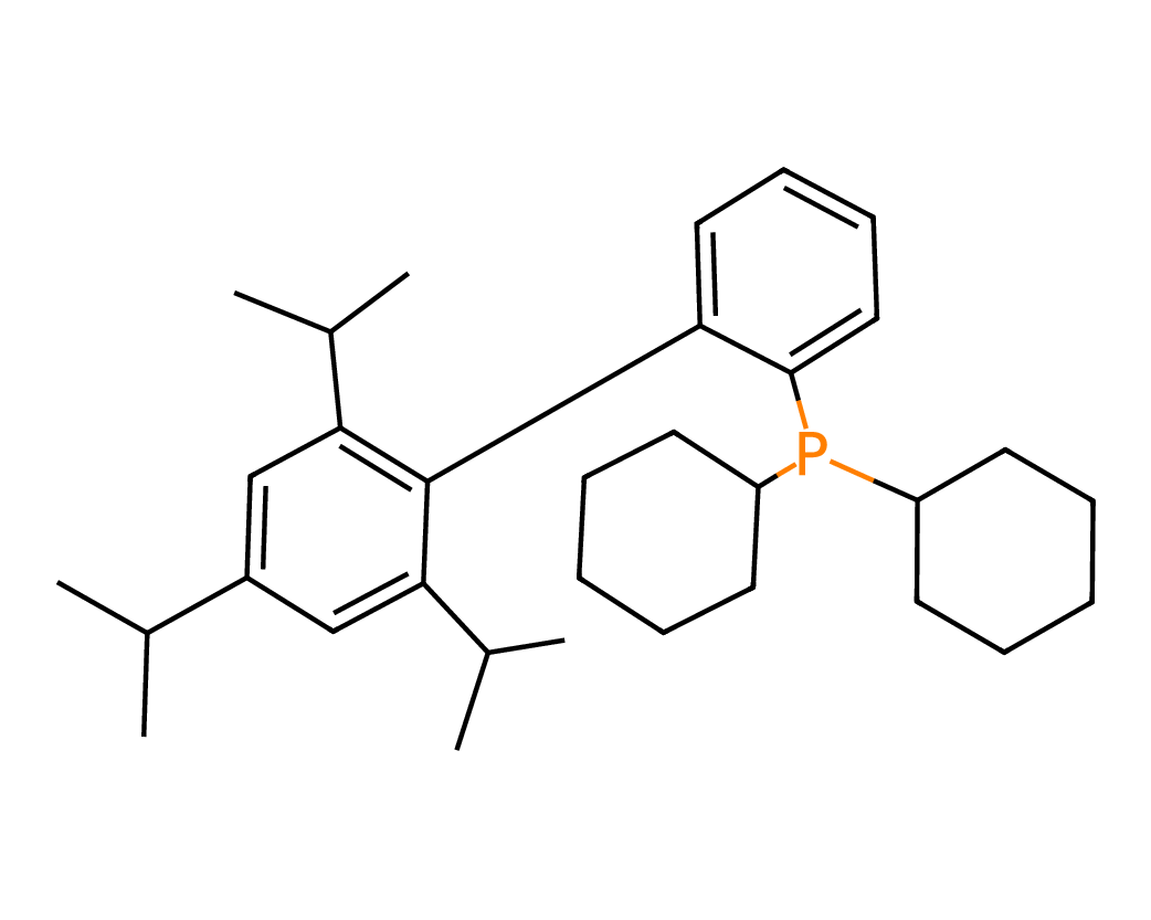
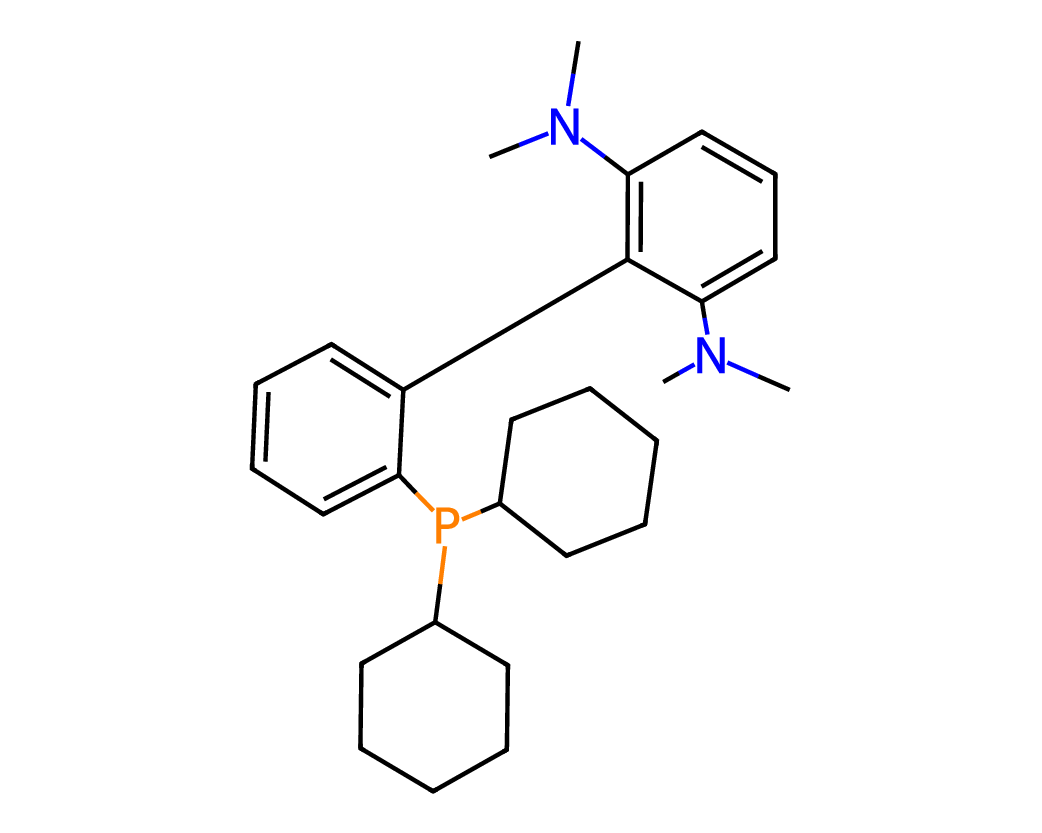
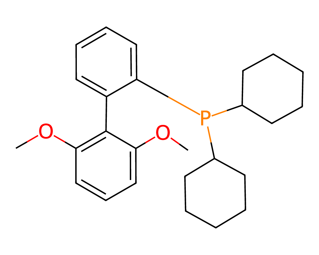
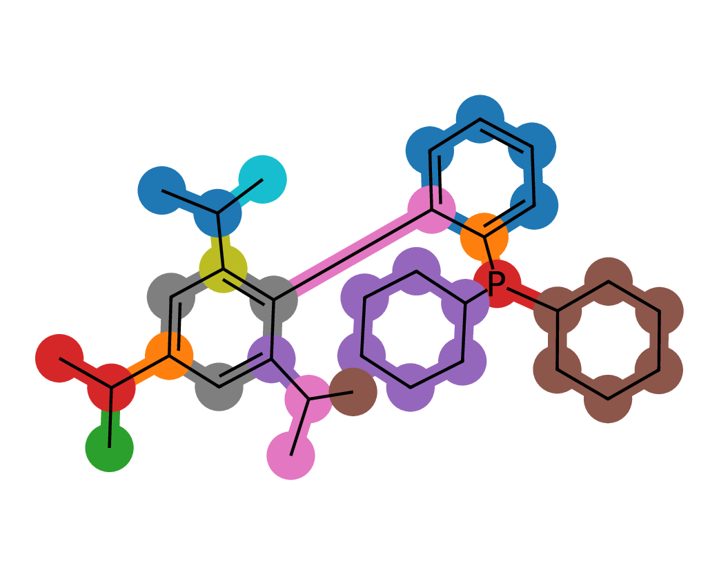
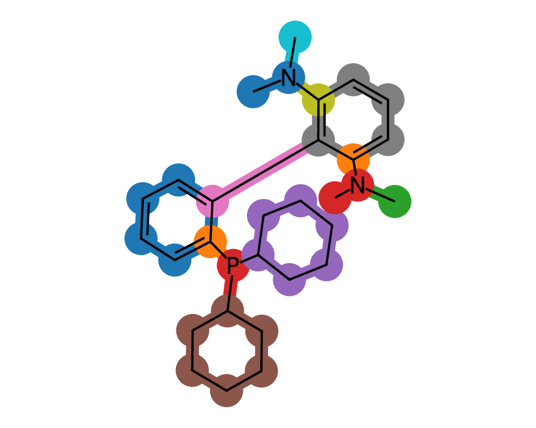
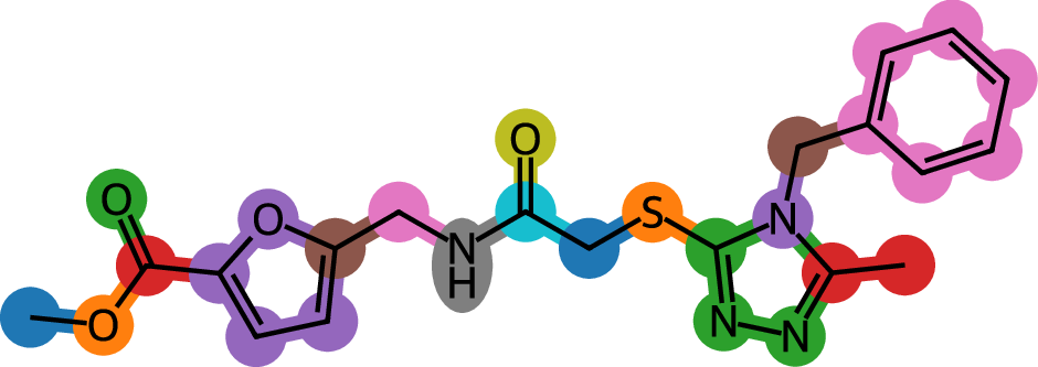
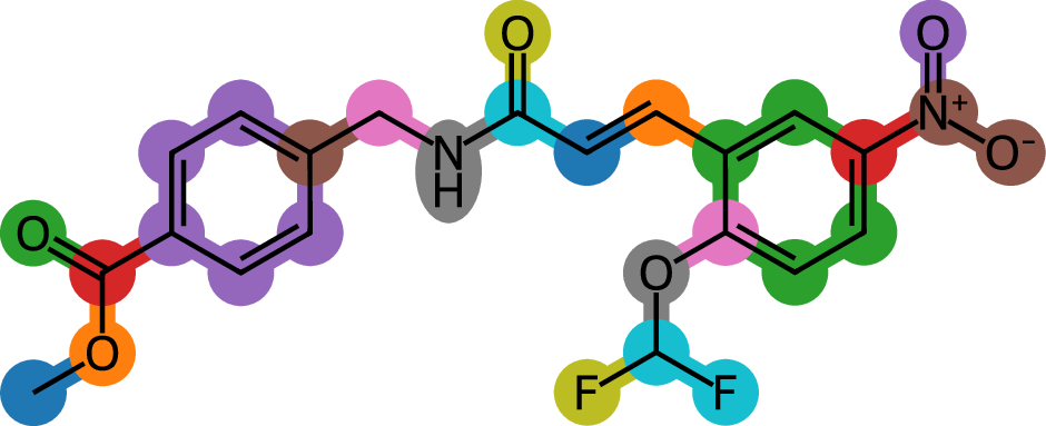
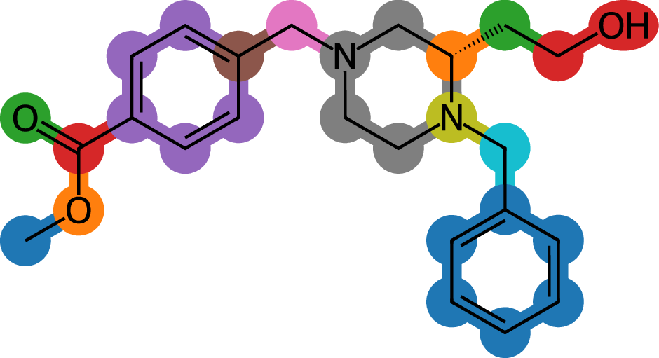
Figures 5 and 6 illustrate representative examples of fragment extraction using the RingPath algorithm on the Kraken and Drug-75k datasets. The top row displays the original 2D molecular structures, while the bottom row shows the corresponding RingPath decompositions. Each colored region highlights a distinct structural fragment, such as a ring or path, demonstrating the algorithm’s ability to segment complex molecules into chemically meaningful and interpretable components.

Appendix C Additional Analysis of FACET’s Scalability and Performance with More 3D Conformers

In this section, we further analyze FACET’s scalability on the following two factors:

C.1 Inference Time when Increasing the Number of 3D Conformers for Each Molecule.

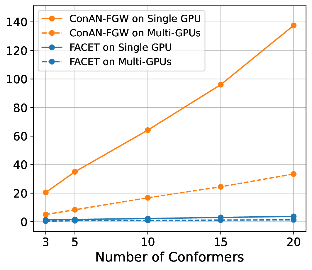
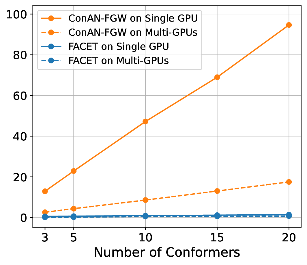
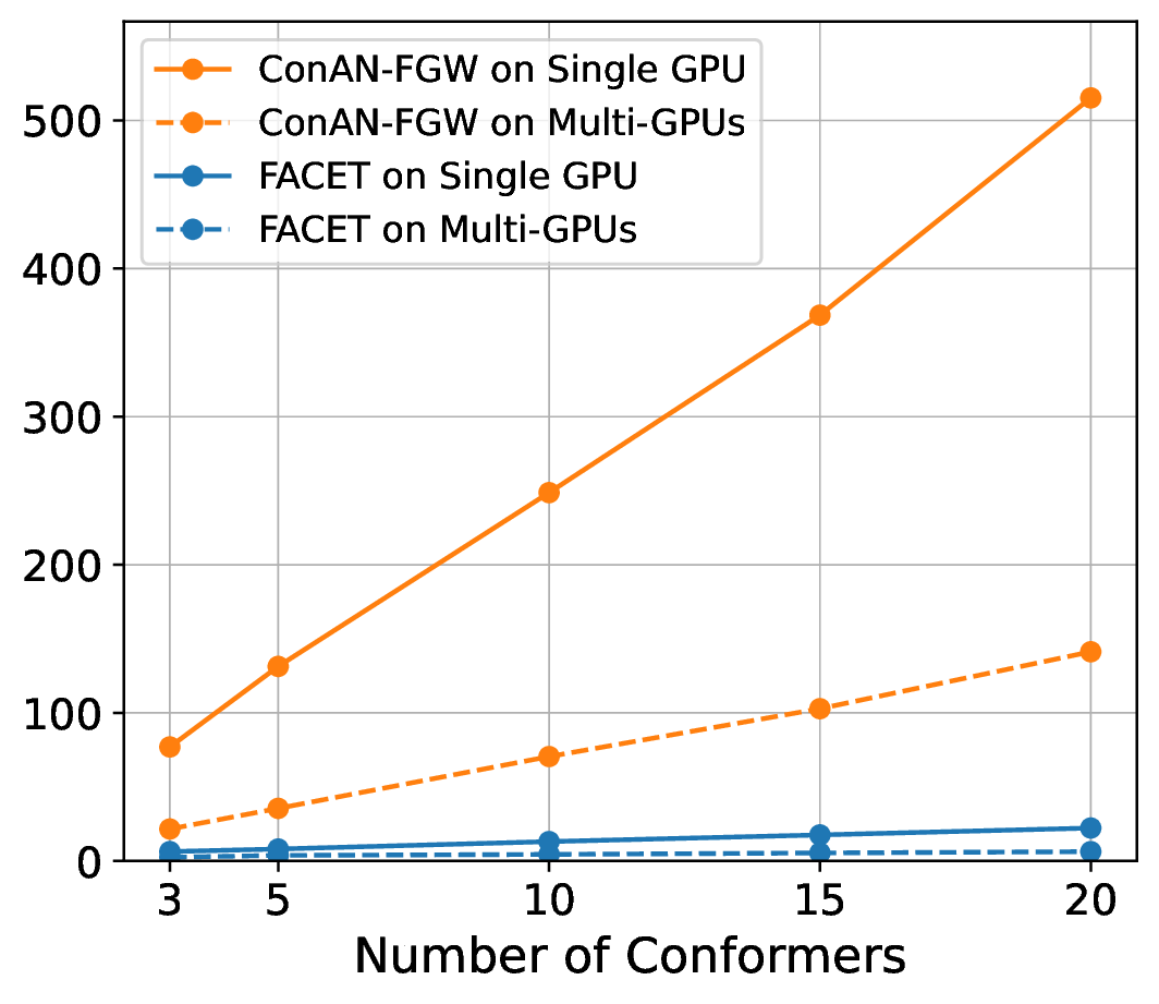
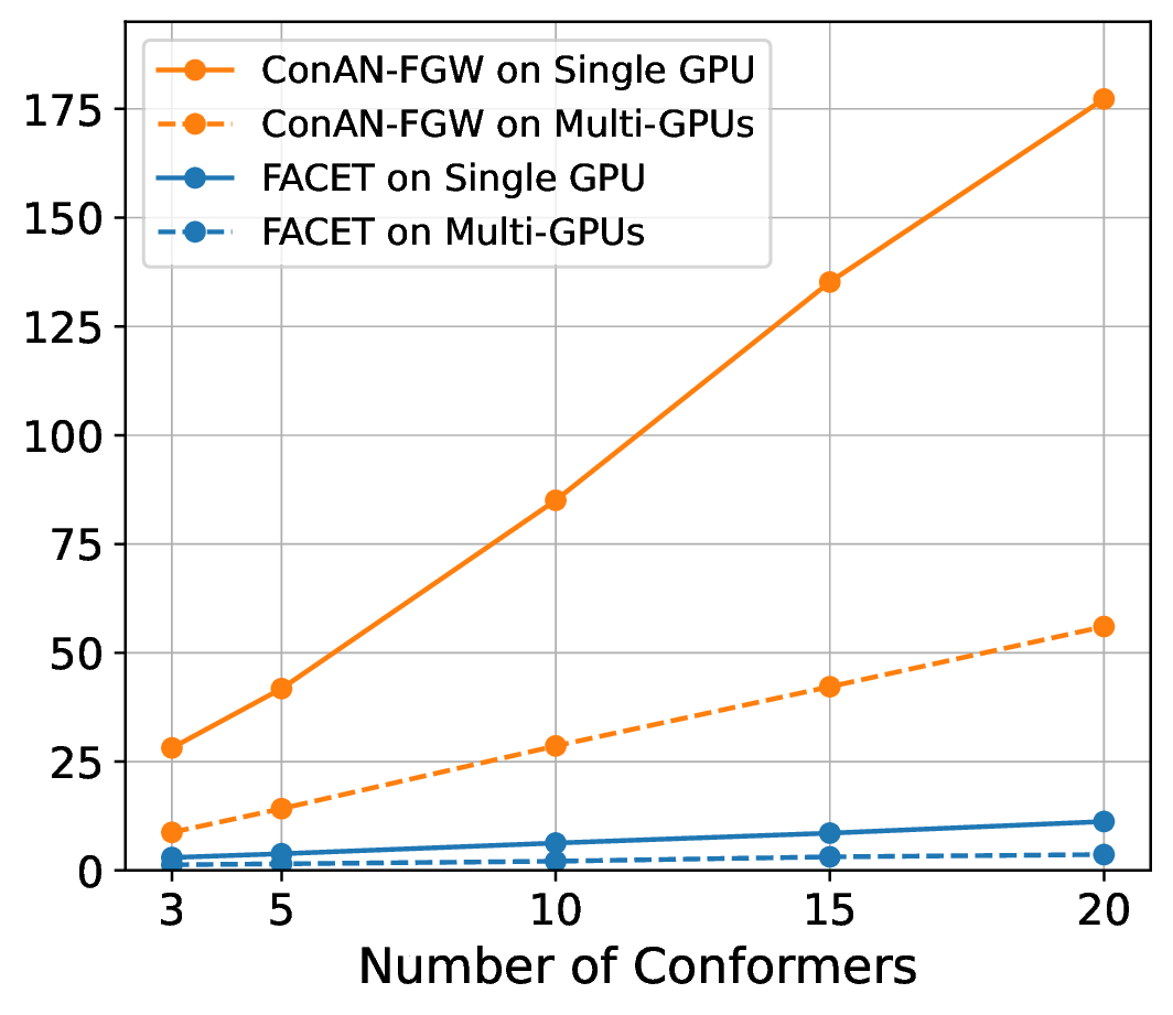
We compare FACET against two versions of ConAN-FGW in running time to extract structure-aware embedding aggregation with different input of 3D conformers. We use two variations of ConAN-FGW, including a single GPU version and another relaxed solver that permits running Sinkhorn iterations on GPUs by matrix multiplication, thus supporting distributed multi-GPUs acceleration. The experiments are conducted on a single GPU using a batch size of $32$ molecules, each with different conformers ranging from $3$ , $5$ , $10$ , $15$ , and $20$ , and another experiment with four GPUs on the same batch size, i.e., 8 molecules per GPU.

Figure 7 indicates our observations across four datasets of MoleculeNet benchmark, where we report the required time to extract embedding aggregations for all molecules in the test set. We see that (i) FACET demonstrates excellent scalability where its runtime remains nearly constant regardless of the number of conformers, both in single-GPU and multi-GPU settings. In contrast, ConAN-FGW shows poor scalability where runtime increases steeply with the number of conformers. While the multi-GPU usage improves runtime over single-GPU, the growth trend remains significant, with runtimes still exceeding 30 seconds at 20 conformers (e.g., with ESOL dataset).

Secondly, the nearly identical runtime of FACET across single- and multi-GPU settings, as shown in the plot, can be attributed to its computational efficiency and the relatively small workload in this experiment. In such cases, the overhead introduced by multi-GPU parallelization - such as inter-GPU communication and data synchronization - can outweigh its potential speedup benefits. Therefore, we argue that multi-GPU acceleration for FACET becomes advantageous only under substantially larger workloads, such as batch processing of thousands to millions of molecules or handling complex input representations that exceed the memory capacity of a single GPU.

C.2 Average Training Time per Epoch as a Function of Dataset Size.

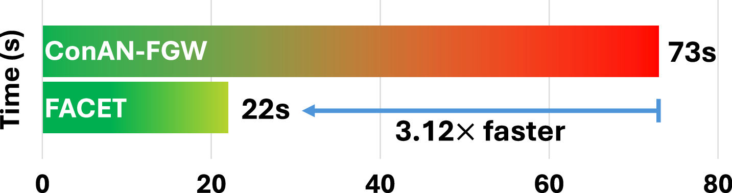
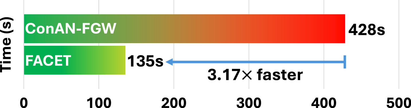
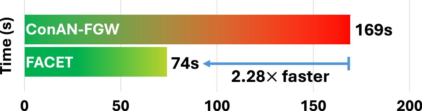
We analyze the scalability of FACET with respect to the number of training molecules. To this end, we report the average training time per epoch across four datasets from the MoleculeNet benchmark. Figure 8 compares the training time of FACET and ConAN-FGW on a single GPU, using a batch size of 256 and 5 conformers per molecule. As shown in the figure, FACET achieves a 2.28× to 3.17× speedup over ConAN-FGW. Notably, this speedup is roughly proportional to the number of training molecules in each dataset, as reported in Table 3.

C.3 Ablation Study on the Impact of Increasing the Number of 3D Conformers in FACET

We provide below a comprehensive ablation study on the impact of using an increasing number of RDKit-generated conformers across four datasets (ESOL, FreeSolv, BACE, and Lipo).

As shown in Table 6, we observe a consistent trend across datasets: increasing the number of conformers from 3 to 5 leads to improved regression performance (lower values indicate better results). However, beyond 5 conformers, the performance tends to converge or slightly fluctuate, confirming that our geometry-aware embedding approach using the FGW distance provides stable and reliable approximations. This aligns with the theoretical expectation that the approximation error scales with $O (1 / K)$ , where $K$ is the number of conformers used.

Table 6: Comparisons on performance with different numbers of conformers generated by RDKit.

Settings	3 conf.	5 conf. (default)	10 conf.	15 conf.	20 conf.
ESOL	0.539 ± 0.06	0.516 ± 0.04	0.501 ± 0.02	0.511 ± 0.03	0.546 ± 0.02
FreeSolv	0.977 ± 0.25	0.967 ± 0.08	0.933 ± 0.23	0.946 ± 0.24	0.949 ± 0.21
BACE	0.542 ± 0.05	0.495 ± 0.03	0.513 ± 0.02	0.519 ± 0.01	0.517 ± 0.03
Lipo	0.445 ± 0.02	0.424 ± 0.01	0.444 ± 0.02	0.447 ± 0.08	0.445 ± 0.01

When 3D conformers generated by RDKit are not used, our FACET model simplifies significantly. In this configuration, the model only receives 2D molecular graphs along with fragment-level information, and key components such as the Graph Transformer are removed. Table 7 presents the performance comparison between the full FACET model and its 2D-only variant across four benchmark datasets:

Table 7: Comparisons on performance without conformers generated by RDKit.

Method	ESOL(↓)	FreeSolv(↓)	BACE(↓)	Lipo(↓)
FACET	0.516 ± 0.04	0.967 ± 0.08	0.495 ± 0.03	0.424 ± 0.01
w/o 3D conformers	0.546 ± 0.03	1.197 ± 0.09	0.584 ± 0.03	0.543 ± 0.02

These results clearly demonstrate that incorporating 3D conformers, even those generated by RDKit, is critical to the expressiveness and performance of FACET. The full model consistently outperforms its 2D-only counterpart, highlighting the importance of 3D geometry in learning accurate molecular representations.

Appendix D Comparison of Training Time between FACET and CoNan-FGW

To provide a comprehensive comparison, we conducted additional experiments to compare the training time of FACET and CoNAN-FGW, with the addition of GemNet, a strong state-of-the-art 3D molecular model, on two benchmark datasets: BACE (1,059 molecules) and LIPO (2,940 molecules). All models were trained for 200 epochs under the same settings. Since both FACET and CoNAN-FGW are originally built on the SchNet architecture, which is generally less expressive than GemNet, we also report the performance of FACET when upgraded to use GemNet as its backbone. From the results listed in Table 8, we have the following key observations:

•
FACET vs. CoNAN-FGW: FACET consistently shows reduced training time compared to CoNAN-FGW, though the degree of reduction varies by dataset size.
- –
  
  On BACE: the time savings are marginal due to the additional cost introduced by the Graph Transformer component in FACET, which is trained using the pre-computed FGW distances from the optimal transport solver.
- –
  
  On LIPO: the training time reduction is more substantial. This is because CoNAN-FGW incurs a high computational cost from directly computing FGW distances between sets of 3D conformers in every forward pass. In contrast, FACET leverages pre-learned geometry-aware embeddings, where the corresponding operation reduces to a lightweight matrix multiplication in the Graph Transformer.
•

FACET vs. GemNet: FACET represents a balanced trade-off between CoNAN-FGW and GemNet in terms of training time. Despite using the simpler SchNet backbone, FACET achieves competitive, sometimes better, performance compared to GemNet, thanks to its geometry-aware aggregation via FGW-based embeddings. This efficiency stems from replacing costly pairwise conformer comparisons with a latent-space transformer that captures 3D geometric information in a more scalable manner.
•

FACET (GemNet) vs. GemNet: When both models share the same GemNet architecture, FACET outperforms GemNet in terms of predictive accuracy on both datasets. We observe that (i) the additional training time incurred by FACET is relatively modest: approximately +21% on BACE and +33% on LIPO, and (ii) given the performance gains, this extra time remains acceptable in practical scenarios and demonstrates FACET’s scalability and effectiveness.

Table 8: Comparisons on performance in terms of MSE(↓) and corresponding training time(↓).

Model	Metric	BACE	LIPO
GemNet	MSE	0.51 ± 0.07	0.45 ± 0.01
	Time	2.04 hours	4.8 hours
Conan-FGW (SchNet)	MSE	0.55 ± 0.02	0.42 ± 0.02
	Time	2.5 hours	6.3 hours
FACET (SchNet)	MSE	0.50 ± 0.03	0.42 ± 0.01
	Time	2.3 hours	5.05 hours
FACET (GemNet)	MSE	0.46 ± 0.03	0.39 ± 0.02
	Time	2.47 hours	6.4 hours

Appendix E Performance of FACET and CoNan-FGW on MARCEL benchmark

To provide a meaningful comparison, we benchmarked FACET against CoNAN-FGW on 10% of the Drug-75k dataset and on the Kraken dataset, which serve as representative subsets. The results (provided below) show that FACET performs competitively or outperforms CoNAN-FGW, even under these reduced-scale settings, reinforcing the efficiency and effectiveness of our approach. The results are shown in Tables 10 and 11.

Appendix F Comparisons with SOTA methods in 2D (or 3D)

FACET is designed as a modular framework for enhancing molecular property prediction by integrating structure-aware aggregation over multiple conformers. A central strength of this design is that it can be plugged into a variety of existing backbone architectures, whether 2D or 3D, thus offering a complementary mechanism rather than an alternative to these models.

FACET improves standalone 3D architectures

We integrated FACET with established 3D models such as SchNet, GemNet, and VisNet, and consistently observed performance improvements across datasets. Table 9 demonstrates that FACET’s geometry-aware aggregation over multiple conformers complements even strong 3D baselines, validating its utility beyond what these models achieve on their own.

Table 9: Comparisons on performance with different standalone 3D architectures.

Model	BACE(↓)	LIPO(↓)
SchNet	0.64 ± 0.05	0.56 ± 0.01
FACET (SchNet)	0.50 ± 0.03	0.42 ± 0.01
GemNet	0.51 ± 0.07	0.45 ± 0.01
FACET (GemNet)	0.46 ± 0.03	0.39 ± 0.02
VisNet	0.61 ± 0.15	0.55 ± 0.45
FACET (VisNet)	0.47 ± 0.01	0.48 ± 0.01

FACET enhances simple 2D MPNNs

We also applied FACET to a lightweight 2D message-passing neural network and found that incorporating FACET’s fragment-level structure-aware aggregation significantly improved performance. This result underscores the compatibility of FACET with 2D backbones and its ability to enhance models that do not explicitly process 3D information.

Appendix G Unified training pipeline

We investigated the performance of the proposed method when combining all training steps into an end-to-end pipeline. Below, we summarize our findings step by step:

•

Step 1 – Pretraining 2D and 3D MPNNs: As suggested in prior work like CoNAN-FGW, we begin by pretraining the 2D and 3D MPNNs independently. This initial phase is critical to ensure that the encoders, especially the 3D MPNN, converge to a stable and meaningful representation before introducing structure-aware aggregation. To test the necessity of this stage, we experimented with a variant where all three stages were co-trained from scratch. The results showed substantially lower performance, confirming that Stage 1 is crucial for learning rich, aligned, and stable representations.
•

Steps 2 and 3 – Co-training Graph Transformer and Downstream Fine-tuning: While our default setup trains Step 2 (Graph Transformer with FGW supervision) and Step 3 (fine-tuning on molecular properties) sequentially, we explored an alternative setup where both steps are co-trained. To manage the computational cost of FGW supervision, we adopted an alternating strategy: after every five steps of property prediction optimization, we update the Graph Transformer to approximate FGW distances. This reduces the training burden compared to full FGW supervision at every iteration (as in CoNAN-FGW).

Table 10: Comparisons of performance between FACET and CoNan-FGW on Kraken

	L	BurL	B5	BurB5
Conan-FGW (SchNet)	0.397	0.117	0.272	0.195
FACET (SchNet)	0.398	0.125	0.251	0.180

Table 11: Comparisons of performance between FACET and CoNan-FGW on Drugs-7.5k

	$χ$	IP	EA
Conan-FGW (SchNet)	0.374	0.541	0.587
FACET (SchNet)	0.365	0.535	0.552

As shown in Table 12, without separately training Step 1, the model got low performance, confirming that this stage helps the model ensure rich, aligned, and stable molecular representations before incorporating more advanced structure awareness. Secondly, on four MoleculeNet datasets, co-training Steps 2 and 3 produced slightly improved performance over the default FACET setup. For example, on ESOL, performance improved from 0.505 to 0.516, and on FreeSolv, from 0.867 to 0.967. This improvement can be attributed to the model’s ability to jointly adapt the 2D/3D encoders and the Graph Transformer, leading to more aligned, task-relevant representations. However, there is a trade-off. This co-training strategy comes with an increased training cost, as FGW distances must still be computed periodically. As a result, while training is slower than the default FACET setup, it remains significantly faster than CoNAN-FGW, and achieves a strong balance between efficiency and predictive performance, especially on large-scale datasets like Drug-75k.

Table 12: Comparisons of performance (MSE

↓

)of different training strategies.

	ESOL(↓)	FreeSolv(↓)	BACE(↓)	Lipo(↓)
ConAN-FGW	0.529 ± 0.022	1.068 ± 0.083	0.549 ± 0.016	0.422 ± 0.016
FACET	0.516 ± 0.044	0.967 ± 0.082	0.495 ± 0.115	0.424 ± 0.009
FACET (Merge all steps)	0.567 ± 0.023	1.264 ± 0.094	0.591 ± 0.062	0.530 ± 0.013
FACET (Merge steps 2-3)	0.505 ± 0.014	0.867 ± 0.102	0.497 ± 0.035	0.44 0± 0.014

Appendix H Limitations of FACET

H.1 FACET Operates on a Predefined Set of 3D Conformers.

Our method enables efficient geometry-aware aggregation without requiring expensive alignment procedures at inference time. While FACET demonstrates improved performance even with a small subset of conformers, the quality and representativeness of this subset can still influence downstream predictions. In particular, if the selected conformers are heavily biased or fail to capture key structural variations, some aspects of molecular flexibility may be underrepresented. Addressing this challenge through better conformer sampling strategies or task-aware selection mechanisms could further enhance model robustness, especially for highly flexible molecules.

Future direction: A promising extension would be to develop end-to-end models that can learn to generate conformers dynamically during training, using gradient feedback from downstream prediction losses. Such a differentiable conformer generation module could enable task-aware structural modeling, ensuring that the generated conformers are optimized not just for physical plausibility, but also for relevance to the predictive task at hand.

H.2 Limitations in Scope: Focus on Small Molecules

FACET has primarily been evaluated on standard molecular property prediction benchmarks such as those in MoleculeNet, which consist mostly of small, drug-like molecules. While this setup is well-suited for many pharmacological applications, it limits the assessment of FACET’s generalizability to more complex molecular systems. For example, biomacromolecules (e.g., peptides, proteins, nucleic acids) exhibit high flexibility, long-range dependencies, and hierarchical organization that are not present in small molecules. Polymers and materials often involve much larger structures without well-defined conformers, challenging FACET’s reliance on discrete 3D inputs. Additionally, FACET currently models only single-molecule properties and has not been extended to multi-molecular interactions, such as protein-ligand binding.

Future direction: To broaden FACET’s applicability, several promising future directions can be explored. First, incorporating efficient attention to capture both local fragment-level information and long-range structural dependencies is essential for handling large biomolecules. Second, adapting FACET to support flexible input formats, such as voxel grids or material-specific graphs, would allow it to process polymers and crystalline materials that lack stable conformers. Third, extending FACET to jointly model molecular interactions through cross-graph attention or co-embedding mechanisms could open applications in drug docking and molecular complex prediction. Finally, applying and evaluating FACET on broader datasets, such as PDBbind (Liu et al., 2015), PolyInfo (Otsuka et al., 2011), or CoRE MOF 2019 (Chung et al., 2019), would provide a more comprehensive understanding of its strengths and limitations across molecular domains.

Appendix I Proof of Theorem 1

Recall that we aim to establish the following novel theoretical bounds: Let $𝑫$ denote the pairwise $FGW_{p, α}$ distance matrix, and let ${λ_{k}, 𝒗_{k}}_{k = 1}^{K}$ represent the eigendecomposition of the associated criterion matrix $𝑭 = - 𝑪 𝑫 𝑪$ , where $𝑪 = 𝑰_{K} - \frac{1}{K} 𝟏_{K} 𝟏_{K}^{⊤}$ is the centering matrix. The optimal stress value, denoted by $𝒮^{*}$ , is bounded as follows: $ℒ \leq 𝒮^{*} \leq 𝒰$ , where

ℒ : = \sum_{k : λ_{k} < 0} λ_{k}^{2}, 𝒰 : = \sum_{k l} (Δ g_{k} + Δ g_{l})^{2} + ℒ + 𝒞, Δ g_{k} = \frac{1}{2} \sum_{l : λ_{l} < 0} λ_{l} \cdot 𝒗_{k l}^{2}, \forall k \in [K] .

Here, $𝒗_{k l}$ denotes the $l$ -th component of the $k$ -th eigenvector $𝒗_{k}$ of $𝑭$ , and $𝒞$ quantifies the approximation error between the empirical barycenter in the Euclidean embedding space and its counterpart in the original space of undirected attributed graphs. This is equivalent to that given $𝒆 : = {𝒆_{k}}_{k \in [K]} \in ℝ^{d \times K}$ , our objective is to derive lower and upper bounds for the following cumulative stress:

$𝒮^{*}$	$= \min_{𝒆 \in ℝ^{d \times K}} 𝒮 (𝒆), 𝒮 (𝒆) = 𝒮_{1} (𝒆) + 𝒮_{2} (𝒆),$	(13)
$𝒮^{*}_{1}$	$: = \min_{𝒆 \in ℝ^{d \times K}} 𝒮_{1} (𝒆), 𝒮_{1} (𝒆) : = \sum_{k, l \in [K]} (∥ 𝒆_{k} - 𝒆_{l} ∥_{2}^{2} - D_{k l})^{2},$	(14)
$𝒮^{*}_{2}$	$: = \min_{𝒆 \in ℝ^{d \times K}} 𝒮_{2} (𝒆), 𝒮_{2} (𝒆) : = \sum_{l \in [K]} (∥ \bar{𝒆}_{K} - 𝒆_{l} ∥_{2}^{2} - \bar{D}_{K, l})^{2} .$	(15)

To this end, we begin by specifying and formally defining the following important concepts in Section I.1.

I.1 Non-Euclidean Nature of Pairwise FGW Distance Matrix

Definition 1 (Euclidean Distance Matrix).

A $K \times K$ distance matrix $𝐃$ is said to be Euclidean if there exists a set of points $𝐞 = {𝐞_{k}}_{k = 1}^{K}$ in some Euclidean space $ℝ^{d}$ such that

\forall k, l \in [K], D_{k l} = ∥ 𝒆_{k} - 𝒆_{l} ∥_{2}^{2} .

The space of all Euclidean distance matrices (EDM) is denoted by $ℰ$ .

Fact 1 (Conditions for Euclidean Distance Matrix, see, e.g., Gower (1985)).

A matrix $𝐃$ is an EDM if and only if it satisfies the following three conditions:

(i)

Non-negativity: $D_{k l} \geq 0$ for all $k, l \in [K]$ ,
(ii)

Hollow diagonal: $D_{k k} = 0$ for all $k \in [K]$ ,
(iii)

Positive semidefiniteness: the associated double-centered matrix $𝑭 : = - 𝑪 𝑫 𝑪$ is positive semidefinite (PSD), where $𝑪 = 𝑰_{K} - \frac{1}{K} 𝟏_{K} 𝟏_{K}^{⊤}$ is the centering matrix, and $𝟏_{K}$ denotes the $K$ -dimensional vector of ones.

Recall that the pairwise FGW distance matrix $𝑫$ for a collection of $K$ distributions is defined entry-wise by $D_{k l} : = FGW_{p, α} (𝒢 (𝕊_{k}), 𝒢 (S_{l}))$ for all $k, l \in [K]$ , as introduced in Section 3. The following result establishes that this matrix does not correspond to a Euclidean distance matrix:

Lemma 1 (Non-Euclidean Nature of Pairwise FGW Distance Matrix).

Consider the case where $d_{f} = ∥ \cdot ∥_{2}$ . Then the FGW distance matrix $𝐃$ , whose entries are given by

FGW_{p, α} (𝒢_{1}, 𝒢_{2}) : = \min_{𝝅 \in Π (𝝎_{1}, 𝝎_{2})} ⟨ (1 - α) 𝑴 + α 𝑳 (𝑨_{1}, 𝑨_{2}) \otimes 𝝅, 𝝅 ⟩,

with $α \in [0, 1]$ , does not define a Euclidean distance matrix.

As established in Lemma 1, which is proved in Section I.4, the distance $FGW_{p, α}$ is not a Euclidean distance. Therefore, we are interested in quantifying how accurately non-Euclidean distance matrices can be approximated by pairwise distances between learned embeddings. To this end, we analyze the lower and upper bound of the set $𝒮$ in Sections I.2 and I.3, respectively.

I.2 Lower Bounds on Embedding non-Euclidean FGW Distances

We would like to find the lower bound of $𝒮$ . We note that the original formulation is non-convex, making it analytically intractable. Nonetheless, by reparameterizing the objective as a function of the pairwise squared distances $\hat{D}_{k l} : = ∥ 𝒆_{k} - 𝒆_{l} ∥_{2}^{2}$ and $\bar{\hat{D}}_{K l} : = ∥ \bar{𝒆}_{K} - 𝒆_{l} ∥_{2}^{2}$ induced by the embedding, and by incorporating the necessary conditions to ensure that $\hat{𝑫}$ corresponds to a valid Euclidean distance matrix, the reformulated problem becomes convex for $𝒮_{1}$ . Note that we can prove that $𝒮$ has a lower bound at $\hat{𝑳}^{*}$ , where $\hat{𝑳}^{*}$ is a minimizer of $𝒮_{1}$ , that is,

	$𝒮^{*}$	$= \min_{\hat{𝑫} \in ℰ} [𝒮_{1} (\hat{𝑫}) + 𝒮_{2} (\hat{𝑫})], 𝒮_{2} (\hat{𝑫}) : = \sum_{l \in [K]} (\bar{\hat{D}}_{K l} - \bar{D}_{K, l})^{2},$		(16)
	$𝒮_{1} (\hat{𝑳}^{*})$	$= \min_{\hat{𝑫} \in ℰ} 𝒮_{1} (\hat{𝑫}), 𝒮_{1} (\hat{𝑫}) : = \sum_{k, l \in [K]} (\hat{D}_{k l} - D_{k l})^{2} .$		(17)

Indeed, given the previous reformulation of $𝒮$ , we can establish the following lower bound via Proposition 1. Notably, to simplify the problem, in Proposition 1, we relax the EDM constraint by considering $ℰ_{ℒ}$ , containing $ℰ$ by keeping only the PSD property from the EDM definition in Fact 1. We will reintroduce the missing constraints in $ℰ_{ℒ}$ and use the solution for the simplified problem to construct an upper bound in Section I.3.

Proposition 1 (Error Lower Bound of $𝒮^{*}$ ).

The lower bound of $𝒮$ is provided as follows:

$𝒮^{*}$	$= \min_{\hat{𝑫} \in ℰ} [𝒮_{1} (\hat{𝑫}) + 𝒮_{2} (\hat{𝑫})] \geq 𝒮_{1} (\hat{𝑳}^{}) + 𝒮_{2} (\hat{𝑳}^{}) \geq ℒ_{1} + ℒ_{2} = : ℒ,$	(18)
$𝒮_{1} (\hat{𝑳}^{*})$	$= \min_{\hat{𝑫} \in ℰ_{ℒ}} 𝒮_{1} (\hat{𝑫}) \geq \sum_{k : λ_{k} < 0} λ_{k}^{2} = : ℒ_{1},$	(19)
$𝒮_{2} (\hat{𝑳}^{*})$	$= \min_{\hat{𝑫} \in ℰ_{ℒ}} 𝒮_{2} (\hat{𝑫}) = 0 = : ℒ_{2} .$	(20)

Here $ℰ_{ℒ}$ contains $ℰ$ by keeping only the PSD property from the EDM definition in Fact 1.

Proof of Proposition 1.

Note that if $𝒮_{1}$ is minimized at $\hat{𝑳}^{*}$ , that is,

𝒮_{1} (\hat{𝑳}^{*})

= \min_{\hat{𝑫} \in ℰ} 𝒮_{1} (\hat{𝑫}), 𝒮_{1} (\hat{𝑫}) : = \sum_{k, l \in [K]} (\hat{D}_{k l} - D_{k l})^{2} .

(21)

We then can find the lower bound of $𝒮^{*} = \min_{\hat{𝑫} \in ℰ} [𝒮_{1} (\hat{𝑫}) + 𝒮_{2} (\hat{𝑫})]$ via the minimizer $\hat{𝑳}^{*}$ .

Using the definition of Frobenius norm and $ℰ_{ℒ}$ , we can obtain:

𝒮_{1} (\hat{𝑳}^{*}) : = \min_{\hat{𝑫} \in ℰ} 𝒮_{1} (\hat{𝑫}) \geq \min_{\hat{𝑫} \in ℰ_{ℒ}} 𝒮_{1} (\hat{𝑫}), 𝒮_{1} (\hat{𝑫}) = ∥ \hat{𝑫} - 𝑫 ∥^{2}_{F},

We then obtain the following decomposition:

	$∥ \hat{𝑫} - 𝑫 ∥^{2}_{F}$	$= ∥ 𝑨 ∥^{2}_{F} + ∥ 𝑩 ∥^{2}_{F}, 𝑨 : = 𝑪 \hat{𝑫} 𝑪 - 𝑪 𝑫 𝑪,$
	$𝑩$	$: = \frac{1}{K} 𝑶 \hat{𝑫} 𝑪 + \frac{1}{K} 𝑪 \hat{𝑫} 𝑶 + \frac{1}{K^{2}} 𝑶 \hat{𝑫} 𝑶 - (\frac{1}{K} 𝑶 𝑫 𝑪 + \frac{1}{K} 𝑪 𝑫 𝑶 + \frac{1}{K^{2}} 𝑶 𝑫 𝑶),$

where $𝑪 = 𝑰_{K} - \frac{1}{K} 𝑶$ is the centering matrix and $𝑶 = 𝟏_{K} 𝟏_{K}^{⊤}$ is the all-ones matrix. Indeed, using the definition of the centering matrix $𝑪 = 𝑰_{K} - \frac{1}{K} 𝑶$ , we have $𝑰_{K} = 𝑪 + \frac{1}{K} 𝑶$ .

∥ \hat{𝑫} - 𝑫 ∥^{2}_{F}

= ∥ 𝑰_{K} \hat{𝑫} 𝑰_{K} - 𝑰_{K} 𝑫 𝑰_{K} ∥^{2}_{F} = ∥ 𝑨 + 𝑩 ∥^{2}_{F} = ∥ 𝑨 ∥^{2}_{F} + ∥ 𝑩 ∥^{2}_{F} + 2 T r (𝑨 𝑩) = ∥ 𝑨 ∥^{2}_{F} + ∥ 𝑩 ∥^{2}_{F},

Here we used the fact that the matrix product is invariant under cyclic permutation:

T r (𝑨 𝑩) = T r (𝑪 (\hat{𝑫} - 𝑫) 𝑪 (\hat{𝑫} - 𝑫) \frac{1}{K} 𝑶) = T r (\frac{1}{K} 𝑶 𝑪 (\hat{𝑫} - 𝑫) 𝑪 (\hat{𝑫} - 𝑫)) = 0,

and

\frac{1}{K} 𝑶 𝑪 = \frac{1}{K} 𝑶 (𝑰_{K} - \frac{1}{K} 𝑶) = \frac{1}{K} 𝑶 - \frac{1}{K^{2}} 𝑶 𝑶 = 0 .

Under only the PSD constraint, the optimal solution $\hat{𝑳}^{*}$ that minimizes $𝒮_{1} (\hat{𝑫})$ can be decomposed as:

\hat{𝑳}^{*} = \hat{𝑳}^{*}_{𝑨} + \hat{𝑳}^{*}_{𝑩},

where $\hat{𝑳}^{*}_{𝑨}$ and $\hat{𝑳}^{*}_{𝑩}$ respectively minimize the terms $∥ 𝑨 ∥_{F}^{2}$ and $∥ 𝑩 ∥_{F}^{2}$ independently.

In particular, using the definition of the centering matrix $𝑪 = 𝑰_{K} - \frac{1}{K} 𝑶$ , the entries of $\hat{𝑳}^{*}_{𝑩}$ are given by:

	$\hat{𝑳}^{*}_{𝑩, k l}$	$: = [\frac{1}{K} 𝑶 𝑫 𝑪 + \frac{1}{K} 𝑪 𝑫 𝑶 + \frac{1}{K^{2}} 𝑶 𝑫 𝑶]_{k l}$
		$= [\frac{1}{K} 𝑶 𝑫 + \frac{1}{K} (𝑶 𝑫)^{⊤} - \frac{1}{K^{2}} 𝑶 𝑫 𝑶]_{k l} = \bar{𝑫}_{k} + \bar{𝑫}_{l} - \bar{𝑫},$

where $\bar{𝑫}_{k}$ denotes the mean of the $k$ -th row (or column) of $𝑫$ , and $\bar{𝑫}$ is the global mean of all elements in $𝑫$ . Therefore, the rows/columns mean of $\hat{𝑳}^{*}_{𝑩}$ equal those of $𝑫$ itself, and hence

\hat{𝑳}^{*}_{𝑩} = a r g m i n_{\hat{𝑫} \in ℰ_{ℒ}} ∥ 𝑩 ∥^{2}_{F}, \min_{\hat{𝑫} \in ℰ_{ℒ}} ∥ 𝑩 ∥^{2}_{F} = 0 .

Therefore,

\min_{\hat{𝑫} \in ℰ_{ℒ}} 𝒮_{2} (\hat{𝑫}) = \min_{\hat{𝑫} \in ℰ_{ℒ}} \sum_{l \in [K]} (\bar{\hat{D}}_{K l} - \bar{D}_{K, l})^{2} = 0 .

Here we used the fact that the matrix $𝑫$ is given by $D_{k l} : = FGW_{p, α} (𝒢 (𝕊_{k}), 𝒢 (S_{l}))$ for all $k, l \in [K]$ and the empirical FGW barycenter is given by

	$\bar{𝒢}_{K}$	$\in a r g m i n_{𝒢 \in 𝒫_{p} (𝛀)} \frac{1}{K} \sum_{l = 1}^{K} FGW_{p, α}^{p} (𝒢, 𝒢 (S_{l})) = a r g m i n_{𝒢 \in 𝒫_{p} (𝛀)} \frac{1}{K} \sum_{l = 1}^{K} FGW_{p, α} (𝒢, 𝒢 (S_{l})),$
	$\bar{D}_{K, l}$	$: = FGW_{p, α} (\bar{𝒢}_{K}, 𝒢 (S_{l})) = \min_{𝒢 \in 𝒫_{p} (𝛀)} \frac{1}{K} \sum_{l = 1}^{K} FGW_{p, α} (𝒢, 𝒢 (S_{l})) (=: column l -th means of 𝑫),$

where $𝒫_{p} (𝛀)$ denotes the space of attributed graphs with finite $p$ -th order FGW distance. To approximate this barycenter in embedding space, we require

∥ \bar{𝒆}_{K} - 𝒆_{l} ∥_{2}^{2} \approx FGW_{p, α} (\bar{𝒢}_{K}, 𝒢 (S_{l})) : = \bar{D}_{K, l} for all l \in [K],

where $\bar{𝒆}_{K} = \frac{1}{K} \sum_{k = 1}^{K} 𝒆_{k}$ is the mean embedding and $𝒆_{k} : = 𝒯_{θ} (𝐇_{k})$ is the learned representation.

Now we would like to find a local analytic solution $\hat{𝑳}^{*}_{𝑨}$ minimizing $∥ 𝑨 ∥_{F}^{2}$ such that the global solution $\hat{𝑳}^{*} = \hat{𝑳}^{*}_{𝑨} + \hat{𝑳}^{*}_{𝑩}$ minimizes both terms $∥ 𝑨 ∥_{F}^{2}$ and $∥ 𝑩 ∥_{F}^{2}$ simultaneously. That is,

	$\min_{\hat{𝑫} \in ℰ_{ℒ}} ∥ 𝑨 ∥_{F}^{2}$	$= \min_{\hat{𝑫} \in ℰ_{ℒ}} ∥ 𝑪 (\hat{𝑳}_{𝑨} + \hat{𝑳}_{𝑩}) 𝑪 - 𝑪 𝑫 𝑪 ∥_{F}^{2}$
		$= ∥ 𝑪 (\hat{𝑳}^{}_{𝑨} + \hat{𝑳}^{}_{𝑩}) 𝑪 - 𝑪 𝑫 𝑪 ∥_{F}^{2} = ∥ 𝑪 \hat{𝑳}^{*}_{𝑨} 𝑪 - 𝑪 𝑫 𝑪 ∥_{F}^{2} .$

Here we used the fact that by definition of $\hat{𝑳}^{*}_{𝑩}$ , it holds that $𝑪 \hat{𝑳}^{*}_{𝑩} 𝑪 = 0$ . Hence, the optimization becomes:

\min_{\hat{𝑫} \in ℰ_{ℒ}} ∥ 𝑪 \hat{𝑳}_{𝑨} 𝑪 - 𝑪 𝑫 𝑪 ∥_{F}^{2} .

This is in fact the problem of computing the nearest PSD approximation $𝑪 \hat{𝑳}_{𝑨} 𝑪$ to a symmetric matrix $𝑪 𝑫 𝑪$ . Using the result from Higham (1988), we find the analytic solution as follows:

\hat{𝑳}^{*}_{𝑨} = - \sum_{k : λ_{k} > 0} λ_{k} 𝒗_{k} 𝒗_{k}^{⊤} .

(22)

Here ${λ_{k}, 𝒗_{k}}_{k \in [K]}$ are the eigenvalues and eigenvectors of $𝑭 = - 𝑪 𝑫 𝑪$ . Because $𝑪 𝑫 𝑪$ has rows/columns means $0$ , the ones vector $𝟏_{K}$ is an eigenvector of $𝑪 𝑫 𝑪$ with eigenvalue $0$ . This leads to $𝟏_{K}$ is also in the null space $\hat{𝑳}^{*}_{𝑨}$ and:

\hat{𝑳}^{*}_{𝑨} = 𝑪 \hat{𝑳}^{*}_{𝑨} 𝑪, \frac{1}{K} 𝑶 \hat{𝑳}^{*}_{𝑨} = \frac{1}{K} (𝑶 \hat{𝑳}^{*}_{𝑨})^{⊤} = 0 .

Therefore,

∥ \hat{𝑳}^{*} - 𝑫 ∥^{2}_{F} = ∥ \hat{𝑳}^{*}_{𝑨} + \hat{𝑳}^{*}_{𝑩} - 𝑫 ∥^{2}_{F} = \sum_{k : λ_{k} < 0} λ_{k}^{2} .

Combining all together, Proposition 1 is derived as follows:

𝒮^{*} \geq \min_{\hat{𝑫} \in ℰ_{ℒ}} ∥ 𝑨 ∥^{2}_{F} + \min_{\hat{𝑫} \in ℰ_{ℒ}} ∥ 𝑩 ∥^{2}_{F} + \min_{\hat{𝑫} \in ℰ_{ℒ}} 𝒮_{2} (\hat{𝑫}) = \sum_{k : λ_{k} < 0} λ_{k}^{2} + 0 + 0 = \sum_{k : λ_{k} < 0} λ_{k}^{2} = : ℒ .

∎

I.3 Upper Bounds on Embedding of Pairwise Empirical FGW Barycenter Distances

As discussed in Section I.2, the lower bound stated in Proposition 1 is derived by simplifying the problem and relaxing the EDM constraint. Specifically, this relaxation involves considering the set $ℰ_{ℒ}$ , which contains $ℰ$ but retains only the PSD requirement from the EDM characterization given in Fact 1. In Proposition 2, we reintroduce the missing constraints excluded in $ℰ_{ℒ}$ and leverage the closed-form solution obtained from the relaxed problem to construct an upper bound under the original EDM constraint set $ℰ$ .

Proposition 2 (Error Upper Bound of $𝒮^{*}$ ).

There exists a matrix $\hat{𝐔}^{*} \in ℰ$ such that the following upper bounds hold:

$𝒮^{*}$	$= \min_{\hat{𝑫} \in ℰ} [𝒮_{1} (\hat{𝑫}) + 𝒮_{2} (\hat{𝑫})] \leq 𝒮_{1} (\hat{𝑼}^{}) + 𝒮_{2} (\hat{𝑼}^{}) \leq 𝒰_{1} + 𝒰_{2} = : 𝒰,$	(23)
$𝒮_{1} (\hat{𝑼}^{*})$	$= \min_{\hat{𝑫} \in ℰ} 𝒮_{1} (\hat{𝑫}) \leq 𝒰_{1} : = \sum_{k : λ_{k} < 0} λ_{k}^{2} + \sum_{k l} (Δ p_{k} + Δ p_{l})^{2},$
$Δ p_{k}$	$= \frac{1}{2} \sum_{l : λ_{l} < 0} λ_{l} \cdot 𝒗_{k l}^{2}, \forall k \in [K]$	(24)
$𝒮_{2} (\hat{𝑼}^{*})$	$= \min_{\hat{𝑫} \in ℰ} 𝒮_{2} (\hat{𝑫}) \leq \sum_{l} (Δ \bar{𝒑}_{l})^{2} = : 𝒰_{2},$	(25)

where the aggregated error term is defined as:

Δ \bar{𝒑}_{l} : = \frac{1}{2 K} \sum_{k = 1}^{K} \sum_{l : λ_{l} < 0} λ_{l} \cdot 𝒗_{k l}^{2} .

We aim to exploit the information derived from the truncation of the negative eigenspace of the matrix $𝑪 𝑫 𝑪$ , specifically the matrix introduced in Eq.(22), defined as:

\hat{𝑳}^{*}_{𝑨} = - \sum_{k : λ_{k} > 0} λ_{k} 𝒗_{k} 𝒗_{k}^{⊤},

where ${λ_{k}, 𝒗_{k}}_{k \in [K]}$ denote the eigenvalues and corresponding eigenvectors of the matrix $𝑭 = - 𝑪 𝑫 𝑪$ .

Recall that the entries of $\hat{𝑳}^{*}_{𝑩}$ are given by:

\hat{𝑳}^{*}_{𝑩, k l}

= [\frac{1}{K} 𝑶 𝑫 + \frac{1}{K} (𝑶 𝑫)^{⊤} - \frac{1}{K^{2}} 𝑶 𝑫 𝑶]_{k l} = \bar{𝑫}_{k} + \bar{𝑫}_{l} - \bar{𝑫} .

As a consequence, the sum $\hat{𝑳}^{*}_{𝑨} + \hat{𝑳}^{*}_{𝑩}$ may not be strictly hollow or PSD when $𝑫$ is not an EDM. To address this, we seek to construct a symmetric matrix $𝑷$ to be added to $\hat{𝑳}^{*}_{𝑨}$ , resulting in the matrix $\hat{𝑼}^{*} : = \hat{𝑳}^{*}_{𝑨} + 𝑷$ , which is both hollow and PSD. This adjustment is designed to avoid any additional penalty on the term $∥ 𝑨 ∥^{2}_{F}$ , though it may introduce some approximation errors in $∥ 𝑩 ∥^{2}_{F}$ and in the quantity $𝒮_{2}$ . These induced errors contribute to the upper bound $𝒰$ for the optimal score $𝒮^{*}$ .

We begin with the requirement that the matrix $𝑷$ does not contribute any additional penalty to the term $∥ 𝑨 ∥_{F}^{2}$ . This can be ensured by imposing the constraint $𝑪 𝑷 𝑪 = 0$ . Under this condition, the matrix $\hat{𝑼}^{*}$ remains a minimizer of $∥ 𝑨 ∥_{F}^{2}$ , as demonstrated below:

	$\min_{\hat{𝑫} \in ℰ_{ℒ}} ∥ 𝑨 ∥_{F}^{2}$	$= \min_{\hat{𝑫} \in ℰ_{ℒ}} ∥ 𝑪 (\hat{𝑳}_{𝑨} + \hat{𝑳}_{𝑩}) 𝑪 - 𝑪 𝑫 𝑪 ∥_{F}^{2}$
		$= ∥ 𝑪 (\hat{𝑳}^{}_{𝑨} + 𝑷 + \hat{𝑳}^{}_{𝑩}) 𝑪 - 𝑪 𝑫 𝑪 ∥_{F}^{2}$
		$= ∥ 𝑪 \hat{𝑳}^{*}_{𝑨} 𝑪 - 𝑪 𝑫 𝑪 ∥_{F}^{2},$

where the final equality holds due to the constraint $𝑪 𝑷 𝑪 = 0$ .

This leads to the condition $(𝑪 𝑷) 𝑪 = 𝑪 (𝑷 𝑪) = 0$ , implying that $𝑪 𝑷$ lies in the left null space of $𝑪$ , and $𝑷 𝑪$ lies in its right null space. As a result, all rows of $𝑷 𝑪$ must be constant, and this expression can be written as:

𝟏_{K} 𝒄^{⊤} = 𝑷 𝑪 = 𝑷 (𝑰_{K} - \frac{1}{K} 𝑶) or 𝑷 = 𝟏_{K} 𝒄^{⊤} + 𝑷 \frac{1}{K} 𝑶,

where $𝒄$ is a column vector to be defined subsequently. Here, we have used the fact that $𝑪$ is the centering matrix defined by $𝑪 = 𝑰_{K} - \frac{1}{K} 𝑶$ .

Multiplying both sides on the left by $\frac{1}{K} 𝑶$ yields:

\frac{1}{K} 𝑶 𝑷 = \frac{1}{K} 𝑶 𝟏_{K} 𝒄^{⊤} + \frac{1}{K} 𝑶 (\frac{1}{K} 𝑷 𝑶) = 𝟏_{K} 𝒄^{⊤} + \frac{1}{K^{2}} 𝑶 𝑷 𝑶 .

This leads to

𝒄^{⊤} = \frac{1}{K} 𝟏_{K}^{⊤} 𝑷 - \frac{1}{K^{2}} 𝟏_{K}^{⊤} 𝑶 𝑷 𝑶 .

Indeed, via the definition of $𝑶 = 𝟏_{K} 𝟏_{K}^{⊤}$ , we can verify this as follows:

	$𝟏_{K} 𝒄^{⊤} + \frac{1}{K^{2}} 𝑶 𝑷 𝑶$	$= 𝟏_{K} (\frac{1}{K} 𝟏_{K}^{⊤} 𝑷 - \frac{1}{K^{2}} 𝟏_{K}^{⊤} 𝑶 𝑷 𝑶) + \frac{1}{K^{2}} 𝑶 𝑷 𝑶$
		$= \frac{1}{K} 𝟏_{K} 𝟏_{K}^{⊤} 𝑷 - \frac{1}{K^{2}} 𝟏_{K} 𝟏_{K}^{⊤} 𝑶 𝑷 𝑶 + \frac{1}{K^{2}} 𝑶 𝑷 𝑶$
		$= \frac{1}{K} 𝟏_{K} 𝟏_{K}^{⊤} 𝑷 - \frac{1}{K^{2}} 𝑶 𝑶 𝑷 𝑶 + \frac{1}{K^{2}} 𝑶 𝑷 𝑶$
		$= \frac{1}{K} 𝑶 𝑷 .$

Hence,

	$𝑷$	$= 𝟏_{K} (\frac{1}{K} 𝟏_{K}^{⊤} 𝑷 - \frac{1}{K^{2}} 𝟏_{K}^{⊤} 𝑶 𝑷 𝑶) + 𝑷 \frac{1}{K} 𝑶$
		$= \frac{1}{K} 𝟏_{K} (𝟏_{K}^{⊤} 𝑷) + \frac{1}{K} (𝑷 𝟏_{K}) 𝟏_{K}^{⊤} - \frac{1}{K^{2}} 𝟏_{K} 𝟏_{K}^{⊤} 𝑶 𝑷 𝑶$

Since $𝑷 𝟏_{K}$ is a column vector, to satisfy this constraint, $𝑷$ must be of the form:

𝑷 = 𝟏_{K} \frac{𝒑^{⊤}}{K} + \frac{𝒑}{K} 𝟏_{K}^{⊤} - \hat{𝒑} \frac{𝟏_{K} 𝟏_{K}^{⊤}}{K},

where $𝒑 \in ℝ^{K}$ is a vector of free parameters, and $\hat{𝒑}$ denotes its average. This construction implies that $𝑷$ has only $K$ degrees of freedom. However, to ensure that $\hat{𝑳}^{*}_{𝑨} + 𝑷$ has zero diagonal (i.e., the resulting matrix is hollow), the diagonal entries of $𝑷$ must satisfy the following $K$ linear constraints:

𝒑_{k} - \frac{1}{2} \hat{𝒑} = - \frac{1}{2} [\hat{𝑳}^{*}_{𝑨}]_{k k}, \forall k \in [K] .

Solving this linear system yields:

	$𝒑_{k}$	$= \frac{1}{2} (\sum_{l : λ_{l} > 0} λ_{l} \cdot 𝒗_{k l}^{2} + \frac{1}{K} \hat{𝒑}),$
	$\hat{𝒑}$	$= \frac{1}{K} \sum_{k = 1}^{K} 𝒑_{k} = \frac{1}{K} \sum_{k = 1}^{K} \sum_{l : λ_{l} > 0} λ_{l} \cdot 𝒗_{k l}^{2},$

where we have used the fact that $\hat{𝑳}^{*}_{𝑨} = - \sum_{l : λ_{l} > 0} λ_{l} 𝒗_{l} 𝒗_{l}^{⊤}$ , and hence its diagonal entries are given by $[\hat{𝑳}^{*}_{𝑨}]_{k k} = - \sum_{l : λ_{l} > 0} λ_{l} \cdot 𝒗_{k l}^{2}$ .

Consequently, the resulting matrix $𝑷$ can be expressed element-wise as:

𝑷_{k, l} = - \frac{[\hat{𝑳}^{*}_{𝑨}]_{k k} + [\hat{𝑳}^{*}_{𝑨}]_{l l}}{2} \geq 0,

where the inequality follows from the fact that $\hat{𝑳}^{*}_{𝑨}$ is negative semi-definite.

In summary, the matrix $\hat{𝑼}^{*} : = \hat{𝑳}^{*}_{𝑨} + 𝑷$ satisfies all three constraints specified in Definition 1.

Although $\hat{𝑼}^{*}$ preserves the value of $∥ 𝑨 ∥_{F}^{2}$ , it differs from $\hat{𝑳}^{*}_{𝑨}$ and introduces approximation errors in the $∥ 𝑩 ∥_{F}^{2}$ term and the $𝒮_{2}$ term. Note that the sum of the untruncated version of $𝑪 𝑫 𝑪$ and the matrix

\frac{1}{K} 𝑶 𝑫 𝑪 + \frac{1}{K} 𝑪 𝑫 𝑶 + \frac{1}{K^{2}} 𝑶 𝑫 𝑶

is equal to $𝑫$ and remains hollow. Recall the decomposition:

	$∥ \hat{𝑫} - 𝑫 ∥_{F}^{2}$	$= ∥ 𝑨 ∥_{F}^{2} + ∥ 𝑩 ∥_{F}^{2}, 𝑨 : = 𝑪 \hat{𝑫} 𝑪 - 𝑪 𝑫 𝑪,$
	$𝑩$	$: = \frac{1}{K} 𝑶 \hat{𝑫} 𝑪 + \frac{1}{K} 𝑪 \hat{𝑫} 𝑶 + \frac{1}{K^{2}} 𝑶 \hat{𝑫} 𝑶$
		$- (\frac{1}{K} 𝑶 𝑫 𝑪 + \frac{1}{K} 𝑪 𝑫 𝑶 + \frac{1}{K^{2}} 𝑶 𝑫 𝑶),$

where $𝑪 = 𝑰_{K} - \frac{1}{K} 𝑶$ is the centering matrix and $𝑶 = 𝟏_{K} 𝟏_{K}^{⊤}$ is the all-ones matrix.

The matrix

\frac{1}{K} 𝑶 𝑫 𝑪 + \frac{1}{K} 𝑪 𝑫 𝑶 + \frac{1}{K^{2}} 𝑶 𝑫 𝑶

can be written similarly to $𝑷$ by including the contributions from the negative eigenvalues, resulting in the matrix $\tilde{𝑷}$ , parameterized by:

	$\tilde{𝒑}_{k}$	$= \frac{1}{2} (\sum_{l} λ_{l} \cdot 𝒗_{k l}^{2} + \frac{1}{K} \tilde{\hat{𝒑}}),$
	$\tilde{\hat{𝒑}}$	$= \frac{1}{K} \sum_{k = 1}^{K} \tilde{𝒑}_{k} = \frac{1}{K} \sum_{k = 1}^{K} \sum_{l} λ_{l} \cdot 𝒗_{k l}^{2} .$

Define the correction due to negative eigenvalues as:

Δ 𝒑_{k} : = \frac{1}{2} \sum_{l : λ_{l} < 0} λ_{l} \cdot 𝒗_{k l}^{2}, \forall k \in [K] .

The resulting error in the $∥ 𝑩 ∥_{F}^{2}$ term is given by:

∥ 𝑩 ∥_{F}^{2}

= ∥ \tilde{𝑷} - 𝑷 ∥_{F}^{2} = \sum_{k, l} (Δ 𝒑_{k} + Δ 𝒑_{l})^{2} .

Furthermore, the contribution to $𝒮_{2}$ is bounded as:

𝒮_{2}

= \min_{\hat{𝑫} \in ℰ} 𝒮_{2} (\hat{𝑫}) = \sum_{l \in [K]} (\bar{\hat{𝑫}}_{K, l} - \bar{𝑫}_{K, l})^{2} \leq \sum_{l} (Δ \bar{𝒑}_{l})^{2} = : 𝒰_{2},

where the aggregated error term is defined as:

Δ \bar{𝒑}_{l} : = \frac{1}{2 K} \sum_{k = 1}^{K} \sum_{l : λ_{l} < 0} λ_{l} \cdot 𝒗_{k l}^{2} .

I.4 Proof of Lemma 1

The proof is proved via leveraging Proposition 8.2 from Peyré et al. (2019), applied to the specific case $α = 0$ , and relies on the relationships among FGW, Wasserstein (W), and Gromov-Wasserstein (GW) distances.

The FGW cost $FGW_{p, α} (𝒢_{1}, 𝒢_{2})$ is defined via two components: the node feature cost matrix $𝑴 [i, j] = d_{f} (𝑯_{1} [i], 𝑯_{2} [j])^{p}$ , and the structural discrepancy tensor $𝑳 (𝑨_{1}, 𝑨_{2}) [i, j, l, m] = | 𝑨_{1} [i, j] - 𝑨_{2} [l, m] |^{p}$ .

Let $𝒢_{1} = (𝑯_{1}, 𝑨_{1}, 𝝎_{1})$ and $𝒢_{2} = (𝑯_{2}, 𝑨_{2}, 𝝎_{2})$ be two attributed graphs with $N_{1}$ and $N_{2}$ nodes, respectively. Their associated probability measures are

μ_{1} = \sum_{k} ω_{1 k} δ_{(𝒙_{1 k}, 𝒂_{1 k})}, μ_{2} = \sum_{l} ω_{2 l} δ_{(𝒙_{2 l}, 𝒂_{2 l})} .

We define the marginals $μ_{𝑯_{1}} = \sum_{k} ω_{k} δ_{𝒙_{k}}$ and $μ_{𝑨_{1}} = \sum_{k} ω_{k} δ_{𝒂_{k}}$ (and analogously for $μ_{𝑯_{2}}$ and $μ_{𝑨_{2}}$ ) as projections of $μ_{1}$ and $μ_{2}$ onto the feature and structural spaces, respectively.

Using these definitions, we introduce the following notation:

$J_{p} (𝑨_{1}, 𝑨_{2}, 𝝅)$	$= \sum_{i j k l} L_{i j k l} (𝑨_{1}, 𝑨_{2})^{p} 𝝅_{i j} 𝝅_{k l},$	(26)
$GW_{p} (μ_{𝑯_{1}}, μ_{𝑯_{2}})^{p}$	$= \min_{𝝅 \in 𝚷 (𝝎_{1}, 𝝎_{2})} J_{p} (𝑨_{1}, 𝑨_{2}, 𝝅),$	(27)
$H_{p} (𝑴, 𝝅)$	$= \sum_{k l} d_{f} (𝒙_{1 k}, 𝒙_{2 l})^{p} 𝝅_{k l},$	(28)
$W_{p} (μ_{𝑨_{1}}, μ_{𝑨_{2}})^{p}$	$= \min_{𝝅 \in 𝚷 (𝝎_{1}, 𝝎_{2})} H_{p} (𝑴, 𝝅) .$	(29)

Let $𝝅 \in 𝚷 (𝝎_{1}, 𝝎_{2})$ be any admissible coupling. If both $μ_{1}$ and $μ_{2}$ are defined over a common metric space $(𝛀, 𝑨, μ)$ , then the FGW distance is given by:

FGW_{p, α} (𝒢_{1}, 𝒢_{2}) : = \min_{𝝅 \in Π (𝝎_{1}, 𝝎_{2})} ⟨ (1 - α) 𝑴 + α 𝑳 (𝑨_{1}, 𝑨_{2}) \otimes 𝝅, 𝝅 ⟩ .

(30)

We now derive the following fundamental identity:

	$𝔼_{p, α} (𝑴, 𝑨_{1}, 𝑨_{2}, 𝝅)$	$: = \sum_{i j k l} [(1 - α) d_{f} (𝒙_{1 k}, 𝒙_{2 l})^{p} + α \| 𝑨_{1} (i, k) - 𝑨_{2} (j, l) \|^{p}] 𝝅_{i j} 𝝅_{k l}$
		$= (1 - α) H_{p} (𝑴, 𝝅) + α J_{p} (𝑨_{1}, 𝑨_{2}, 𝝅) .$		(31)

Moreover, let $𝝅_{α}$ denote the optimal coupling that minimizes the FGW objective $𝔼_{p, α} (𝑴, 𝑨_{1}, 𝑨_{2}, \cdot)$ . Then the FGW distance admits the following decomposition:

$FGW_{p, α}^{p} (μ_{1}, μ_{2})$	$= \min_{𝝅 \in 𝚷 (𝝎_{1}, 𝝎_{2})} 𝔼_{p, α} (𝑴, 𝑨_{1}, 𝑨_{2}, 𝝅) = 𝔼_{p, α} (𝑴, 𝑨_{1}, 𝑨_{2}, 𝝅_{α})$
	$= (1 - α) H_{p} (𝑴, 𝝅_{α}) + α J_{p} (𝑨_{1}, 𝑨_{2}, 𝝅_{α})$
	$\geq (1 - α) W_{p}^{p} (μ_{𝑨_{1}}, μ_{𝑨_{2}}) + α GW_{p}^{p} (μ_{𝑯_{1}}, μ_{𝑯_{2}}) .$	(32)

This inequality follows from the optimality of the W and GW distances with respect to the cost functions $H_{p}$ and $J_{p}$ , respectively, and highlights the interpolation nature of the FGW distance between these two metrics as governed by the parameter $α$ .

The generalized FGW cost $𝔼_{p, α} (𝑴, 𝑨_{1}, 𝑨_{2}, 𝝅)$ admits the following explicit formulation:

	$𝔼_{p, α} (𝑴, 𝑨_{1}, 𝑨_{2}, 𝝅)$	$= ⟨ (1 - α) 𝑴^{p} + α 𝑳 (𝑨_{1}, 𝑨_{2})^{p} \otimes 𝝅, 𝝅 ⟩$
		$= \sum_{i, j, k, l} [(1 - α) d_{f} (𝒙_{1 k}, 𝒙_{2 l})^{p} + α \| 𝑨_{1} (i, k) - 𝑨_{2} (j, l) \|^{p}] 𝝅_{i j} 𝝅_{k l} .$

Based on the formulation above, we obtain the following upper bound on the FGW distance:

	$FGW_{p, α} (G_{1}, G_{2})$	$\leq ⟨ (1 - α) 𝑴 + α 𝑳 (𝑨_{1}, 𝑨_{2}) \otimes 𝝅, 𝝅 ⟩$
		$\leq \sum_{k, l} [(1 - α) d_{f} (𝒙_{1 k}, 𝒙_{2 l}) + 2^{p - 1} α 𝑨 [k, l]]^{p} 𝝅_{k l},$		(33)

where the second inequality follows from the convexity of the function $x \mapsto x^{p}$ for $p \geq 1$ and an application of Minkowski-type bounds on the structural term. Importantly, inequality in Eq.(33) holds for any admissible coupling $𝝅 \in 𝚷 (𝝎_{1}, 𝝎_{2})$ , and in particular, it remains valid when $𝝅 = \bar{𝝅}$ , the optimal coupling associated with the Wasserstein distance $W_{p} (μ_{1}, μ_{2})$ over the product metric space $(𝛀, \bar{d})$ . Here, the effective distance $\bar{d}$ between structured nodes $(𝒙_{1}, 𝒂_{1})$ and $(𝒙_{2}, 𝒂_{2})$ is defined as:

\bar{d} ((𝒙_{1}, 𝒂_{1}), (𝒙_{2}, 𝒂_{2})) = (1 - α) d_{f} (𝒙_{1}, 𝒙_{2}) + 2^{p - 1} α 𝑨 (𝒂_{1}, 𝒂_{2}) .

Combining this with the Wasserstein formulation in Eq.(29), we observe the following inequality:

FGW_{p, α} (𝒢_{1}, 𝒢_{2}) \leq W_{p} (μ_{𝑨_{1}}, μ_{𝑨_{2}}), and FGW_{p, α} (𝒢_{1}, 𝒢_{2}) = W_{p} (μ_{𝑨_{1}}, μ_{𝑨_{2}}) when α = 0 .

(34)

Appendix J E(3) Invariant Property

We utilize a 2D-MPNN, where node embeddings are iteratively refined across layers as follows:

𝐡_{v}^{ℓ} = 𝖴 𝖯 𝖣^{ℓ} (𝐡_{v}^{ℓ - 1}, 𝖠 𝖦 𝖦^{ℓ} ({𝐌^{ℓ} (𝐡_{v}^{ℓ - 1}, 𝐡_{u}^{ℓ - 1}, 𝒆_{v, u}) : u \in N (v)})),

(35)

with $𝐌^{ℓ}$ denoting the message function, $𝖠 𝖦 𝖦^{ℓ}$ representing aggregation by summation, and $𝖴 𝖯 𝖣^{ℓ}$ implemented as either the identity function or a multilayer perceptron. The final atom-level representation is obtained by integrating three modalities: the 2D molecular graph embeddings $𝐇_{2 D}$ , the 3D conformational features $𝐇_{3 D}$ , and the geometry-based structural descriptors $𝐇_{G T}$ . This fusion is performed using trainable linear projections:

𝐇_{c o m b} = \tilde{𝐖}_{2 D} 𝐇_{2 D} + \tilde{𝐖}_{3 D} 𝐇_{3 D} + \tilde{𝐖}_{G T} 𝐇_{G T},

(36)

where $\tilde{𝐖}_{2 D}, \tilde{𝐖}_{3 D},$ and $\tilde{𝐖}_{G T}$ are trainable parameter matrices. Assuming that $𝐇_{2 D}$ and $𝐇_{G T}$ are composed of $K$ repeated copies of their respective feature vectors, we compute the fused representation as:

𝐇_{c o m b} = \tilde{𝐖}_{2 D} 𝐇_{2 D} + \tilde{𝐖}_{3 D} 𝐇_{3 D} + γ \tilde{𝐖}_{G T} 𝐇_{G T},

(37)

where $γ$ is a hyperparameter controlling the influence of the barycenter features. This fusion scheme allows balanced contributions from all modalities, which is empirically beneficial.

To predict the molecular property, we perform a mean pooling over the $K$ conformations and apply a linear transformation:

\hat{𝒚} = 𝐖^{𝒢} (\frac{1}{K} \sum_{k = 1}^{K} 𝐇_{c o m b} [k]) + 𝐛^{𝒢},

(38)

where $𝐖^{𝒢}$ and $𝐛^{𝒢}$ are the weight matrix and bias vector used for the final prediction.

We demonstrate that the function specified in Eq.(35) through Eq.(38)remains invariant under both the action of the $E (3)$ and permutations of the input conformers.

Theorem 2 (E(3) Invariant Property).

Let $𝒢$ denote the 2D molecular graph, and let $(𝕊_{1}, \dots, 𝕊_{K})$ be a collection of $K$ conformers, where each $𝕊_{k} = {𝐫_{k, n}, Z_{k, n}}_{n = 1}^{N}$ for $k \in [K]$ . Consider the function $\hat{𝐲} = f_{𝛉} (𝒢, (𝕊_{1}, \dots, 𝕊_{K}))$ as defined by Eq.(35) to Eq.(38). Then, for any transformations $g_{1}, \dots, g_{K} \in E (3)$ , the following holds:

f_{𝜽} (𝒢, (g_{1} 𝕊_{1}, \dots, g_{K} 𝕊_{K})) = f_{𝜽} (𝒢, (𝕊_{1}, \dots, 𝕊_{K})) .

Furthermore, for any permutation $π \in S y m ([K])$ , we have:

f_{𝜽} (𝒢, (S_{π (1)}, \dots, S_{π (K)})) = f_{𝜽} (𝒢, (𝕊_{1}, \dots, 𝕊_{K})) .

Proof of Theorem 2.

We establish the result in several steps. First, we consider the invariance properties of the geometric representation $𝐇_{G T}$ . By construction, the geometry-aware embedding aggregation used to obtain $\bar{𝐇} = 𝔼 ({𝒯_{θ} (𝐇_{i})}_{i = 1}^{K}),$ is invariant under permutation of conformers. Additionally, because $E (3)$ transformations preserve Euclidean distances and given that the upstream 3D MPNN is assumed to be $E (3)$ -invariant, the generated features $𝐇_{i}$ are likewise invariant under such transformations.

Next, consider the aggregated representation defined in Eq.(37):

𝐇_{c o m b} = \tilde{𝐖}_{2 D} 𝐇_{2 D} + \tilde{𝐖}_{3 D} 𝐇_{3 D} + \tilde{𝐖}_{G T} 𝐇_{G T} .

From the prior step, we know that $𝐇_{G T}$ is invariant under both $E (3)$ actions and conformer permutations. Additionally, $𝐇_{3 D}$ inherits $E (3)$ invariance from the 3D MPNN and is permutation equivariant, i.e., permuting the conformer inputs permutes the columns of $𝐇_{3 D}$ accordingly. However, because the final prediction in Eq.(38) is based on an average over the conformer-wise features:

\hat{𝒚} = 𝐖^{𝒢} (\frac{1}{K} \sum_{k = 1}^{K} 𝐇_{c o m b} [k]) + 𝐛^{𝒢} .

which is invariant to column permutations of the matrix $𝐇_{3 D}$ , leading to the final $\hat{𝒚}$ is invariant to $E (3)$ group and permutation of 3D conformers. ∎

[bib.bib1] Ahmad et al. (2022) Walid Ahmad, Elana Simon, Seyone Chithrananda, Gabriel Grand, and Bharath Ramsundar. Chemberta-2: Towards chemical foundation models, 2022. ↩ a b

[bib.bib2] Amos et al. (2023) Brandon Amos, Samuel Cohen, Giulia Luise, and Ievgen Redko. Meta optimal transport. International Conference on Machine Learning, 2023. ↩ a

[bib.bib3] Axelrod & Gomez-Bombarelli (2022) Simon Axelrod and Rafael Gomez-Bombarelli. Geom, energy-annotated molecular conformations for property prediction and molecular generation. Scientific Data, 9(1):185, 2022. ↩ a

[bib.bib4] Axelrod & Gomez-Bombarelli (2023) Simon Axelrod and Rafael Gomez-Bombarelli. Molecular machine learning with conformer ensembles. Machine Learning: Science and Technology, 4(3):035025, 2023. ↩ a

[bib.bib5] Axelrod & Gómez-Bombarelli (2023) Simon Axelrod and Rafael Gómez-Bombarelli. Molecular machine learning with conformer ensembles. Mach. Learn.: Sci. Technol., 4(3):035025, September 2023. ISSN 2632-2153. doi: 10.1088/2632-2153/acefa7. ↩ a

[bib.bib6] Bachmann et al. (2022) Fynn Bachmann, Philipp Hennig, and Dmitry Kobak. Wasserstein t-sne. In Joint European Conference on Machine Learning and Knowledge Discovery in Databases, pp. 104–120. Springer, 2022. ↩ a

[bib.bib7] Balaban (1985) Alexandru T Balaban. Applications of graph theory in chemistry. Journal of chemical information and computer sciences, 25(3):334–343, 1985. ↩ a

[bib.bib8] Batatia et al. (2022) Ilyes Batatia, David P Kovacs, Gregor Simm, Christoph Ortner, and Gabor Csanyi. Mace: Higher order equivariant message passing neural networks for fast and accurate force fields. In S. Koyejo, S. Mohamed, A. Agarwal, D. Belgrave, K. Cho, and A. Oh (eds.), Advances in Neural Information Processing Systems, volume 35, pp. 11423–11436. Curran Associates, Inc., 2022. ↩ a

[bib.bib9] Batatia et al. (2023) Ilyes Batatia, Philipp Benner, Yuan Chiang, Alin M. Elena, Dávid P. Kovács, Janosh Riebesell, Xavier R. Advincula, Mark Asta, William J. Baldwin, Noam Bernstein, Arghya Bhowmik, Samuel M. Blau, Vlad Cărare, James P. Darby, Sandip De, Flaviano Della Pia, Volker L. Deringer, Rokas Elijošius, Zakariya El-Machachi, Edvin Fako, Andrea C. Ferrari, Annalena Genreith-Schriever, Janine George, Rhys E. A. Goodall, Clare P. Grey, Shuang Han, Will Handley, Hendrik H. Heenen, Kersti Hermansson, Christian Holm, Jad Jaafar, Stephan Hofmann, Konstantin S. Jakob, Hyunwook Jung, Venkat Kapil, Aaron D. Kaplan, Nima Karimitari, Namu Kroupa, Jolla Kullgren, Matthew C. Kuner, Domantas Kuryla, Guoda Liepuoniute, Johannes T. Margraf, Ioan-Bogdan Magdău, Angelos Michaelides, J. Harry Moore, Aakash A. Naik, Samuel P. Niblett, Sam Walton Norwood, Niamh O’Neill, Christoph Ortner, Kristin A. Persson, Karsten Reuter, Andrew S. Rosen, Lars L. Schaaf, Christoph Schran, Eric Sivonxay, Tamás K. Stenczel, Viktor Svahn, Christopher Sutton, Cas van der Oord, Eszter Varga-Umbrich, Tejs Vegge, Martin Vondrák, Yangshuai Wang, William C. Witt, Fabian Zills, and Gábor Csányi. A foundation model for atomistic materials chemistry, 2023. ↩ a

[bib.bib10] Batzner et al. (2022) Simon Batzner, Albert Musaelian, Lixin Sun, Mario Geiger, Jonathan P. Mailoa, Mordechai Kornbluth, Nicola Molinari, Tess E. Smidt, and Boris Kozinsky. E(3)-equivariant graph neural networks for data-efficient and accurate interatomic potentials. Nat. Commun., 13(1):2453, May 2022. ISSN 2041-1723. ↩ a

[bib.bib11] Chan et al. (2024) Bill WGL Chan, Nicholas B Lynch, Wendy Tran, Jack M Joyce, G Paul Savage, Wim Meutermans, Andrew P Montgomery, and Michael Kassiou. Fragment-based drug discovery for disorders of the central nervous system: designing better drugs piece by piece. Frontiers in Chemistry, 12:1379518, 2024. ↩ a

[bib.bib12] Chithrananda et al. (2020) Seyone Chithrananda, Gabriel Grand, and Bharath Ramsundar. Chemberta: Large-scale self-supervised pretraining for molecular property prediction, 2020. ↩ a

[bib.bib13] Choudhary et al. (2022) Kamal Choudhary, Brian DeCost, Chi Chen, Anubhav Jain, Francesca Tavazza, Ryan Cohn, Cheol Woo Park, Alok Choudhary, Ankit Agrawal, Simon J. L. Billinge, Elizabeth Holm, Shyue Ping Ong, and Chris Wolverton. Recent advances and applications of deep learning methods in materials science. npj Comput. Mater., 8(1):59, Apr 2022. ISSN 2057-3960. ↩ a

[bib.bib14] Chung et al. (2019) Yongchul G Chung, Emmanuel Haldoupis, Benjamin J Bucior, Maciej Haranczyk, Seulchan Lee, Hongda Zhang, Konstantinos D Vogiatzis, Marija Milisavljevic, Sanliang Ling, Jeffrey S Camp, et al. Advances, updates, and analytics for the computation-ready, experimental metal–organic framework database: Core mof 2019. Journal of Chemical & Engineering Data, 64(12):5985–5998, 2019. ↩ a

[bib.bib15] Cormen et al. (2022) Thomas H Cormen, Charles E Leiserson, Ronald L Rivest, and Clifford Stein. Introduction to algorithms. MIT press, 2022. ↩ a

[bib.bib16] Courty et al. (2017) Nicolas Courty, Rémi Flamary, and Mélanie Ducoffe. Learning wasserstein embeddings. International Conference on Learning Representations (ICLR), 2017. ↩ a

[bib.bib17] Cuturi (2013) Marco Cuturi. Sinkhorn distances: Lightspeed computation of optimal transport. Advances in neural information processing systems, 26, 2013. ↩ a

[bib.bib18] Cuturi et al. (2020) Marco Cuturi, Olivier Teboul, Jonathan Niles-Weed, and Jean-Philippe Vert. Supervised quantile normalization for low rank matrix factorization. In International Conference on Machine Learning, pp. 2269–2279. PMLR, 2020. ↩ a

[bib.bib19] Degen et al. (2008) Jorg Degen, Christof Wegscheid-Gerlach, Andrea Zaliani, and Matthias Rarey. On the art of compiling and using’drug-like’chemical fragment spaces. ChemMedChem, 3(10):1503, 2008. ↩ a

[bib.bib20] Du et al. (2022) Weitao Du, He Zhang, Yuanqi Du, Qi Meng, Wei Chen, Nanning Zheng, Bin Shao, and Tie-Yan Liu. Se (3) equivariant graph neural networks with complete local frames. In International Conference on Machine Learning, pp. 5583–5608. PMLR, 2022. ↩ a

[bib.bib21] Du et al. (2023) Yuanqi Du, Limei Wang, Dieqiao Feng, Guifeng Wang, Shuiwang Ji, Carla P Gomes, Zhi-Ming Ma, et al. A new perspective on building efficient and expressive 3d equivariant graph neural networks. Advances in neural information processing systems, 36:66647–66674, 2023. ↩ a

[bib.bib22] Fang et al. (2021) Xiaomin Fang, Lihang Liu, Jieqiong Lei, Donglong He, Shanzhuo Zhang, Jingbo Zhou, Fan Wang, Hua Wu, and Haifeng Wang. Chemrl-gem: Geometry enhanced molecular representation learning for property prediction. Nature Machine Intelligence, 2021. doi: 10.48550/ARXIV.2106.06130. ↩ a

[bib.bib23] Fang et al. (2022) Xiaomin Fang, Lihang Liu, Jieqiong Lei, Donglong He, Shanzhuo Zhang, Jingbo Zhou, Fan Wang, Hua Wu, and Haifeng Wang. Geometry-enhanced molecular representation learning for property prediction. Nature Machine Intelligence, 4(2):127–134, 2022. ↩ a

[bib.bib24] Fedik et al. (2022) Nikita Fedik, Roman Zubatyuk, Maksim Kulichenko, Nicholas Lubbers, Justin S. Smith, Benjamin Nebgen, Richard Messerly, Ying Wai Li, Alexander I. Boldyrev, Kipton Barros, Olexandr Isayev, and Sergei Tretiak. Extending machine learning beyond interatomic potentials for predicting molecular properties. Nat. Rev. Chem., 6(9):653–672, Sep 2022. ISSN 2397-3358. doi: 10.1038/s41570-022-00416-3. ↩ a

[bib.bib25] Feydy et al. (2019) Jean Feydy, Thibault Séjourné, François-Xavier Vialard, Shun-ichi Amari, Alain Trouvé, and Gabriel Peyré. Interpolating between optimal transport and mmd using sinkhorn divergences. In The 22nd International Conference on aRtIfIcIaL InTeLlIgEnCe and Statistics, pp. 2681–2690. PMLR, 2019. ↩ a

[bib.bib26] Gasteiger et al. (2021) Johannes Gasteiger, Florian Becker, and Stephan Günnemann. Gemnet: Universal directional graph neural networks for molecules. Advances in Neural Information Processing Systems, 34:6790–6802, 2021. ↩ a

[bib.bib27] Genevay et al. (2018) Aude Genevay, Gabriel Peyré, and Marco Cuturi. Learning generative models with sinkhorn divergences. In International Conference on Artificial Intelligence and Statistics, pp. 1608–1617. PMLR, 2018. ↩ a

[bib.bib28] Geng et al. (2023) Zijie Geng, Shufang Xie, Yingce Xia, Lijun Wu, Tao Qin, Jie Wang, Yongdong Zhang, Feng Wu, and Tie-Yan Liu. De novo molecular generation via connection-aware motif mining. arXiv preprint arXiv:2302.01129, 2023. ↩ a b

[bib.bib29] Gilmer et al. (2017) Justin Gilmer, Samuel S. Schoenholz, Patrick F. Riley, Oriol Vinyals, and George E. Dahl. Neural message passing for quantum chemistry. In International Conference on Machine Learning, pp. 1263–1272, 2017. ↩ a

[bib.bib30] Gower (1985) J.C. Gower. Properties of Euclidean and non-Euclidean distance matrices. Linear Algebra and its Applications, 67:81–97, June 1985. ISSN 0024-3795. doi: 10.1016/0024-3795(85)90187-9. ↩ a

[bib.bib31] Haviv et al. (2024) Doron Haviv, Russell Zhang Kunes, Thomas Dougherty, Cassandra Burdziak, Tal Nawy, Anna Gilbert, and Dana Pe’Er. Wasserstein Wormhole: Scalable Optimal Transport Distance with Transformer. In Ruslan Salakhutdinov, Zico Kolter, Katherine Heller, Adrian Weller, Nuria Oliver, Jonathan Scarlett, and Felix Berkenkamp (eds.), Proceedings of the 41st International Conference on Machine Learning, volume 235 of Proceedings of Machine Learning Research, pp. 17697–17718. PMLR, July 2024. ↩ a b c

[bib.bib32] Hawkins (2017) Paul CD Hawkins. Conformation generation: the state of the art. Journal of chemical information and modeling, 57(8):1747–1756, 2017. ↩ a

[bib.bib33] Hetzel et al. (2023) Leon Hetzel, Johanna Sommer, Bastian Rieck, Fabian Theis, and Stephan Günnemann. MAGNet: Motif-agnostic generation of molecules from shapes. arXiv preprint arXiv:2305.19303, 2023. ↩ a

[bib.bib34] Higham (1988) Nicholas J. Higham. Computing a nearest symmetric positive semidefinite matrix. Linear Algebra and its Applications, 103:103–118, May 1988. ISSN 0024-3795. doi: 10.1016/0024-3795(88)90223-6. ↩ a

[bib.bib35] Hu et al. (2020a) Weihua Hu, Matthias Fey, Marinka Zitnik, Yuxiao Dong, Hongyu Ren, Bowen Liu, Michele Catasta, and Jure Leskovec. Open graph benchmark: Datasets for machine learning on graphs. Advances in neural information processing systems, 33:22118–22133, 2020a. ↩ a

[bib.bib36] Hu et al. (2020b) Weihua Hu, Bowen Liu, Joseph Gomes, Marinka Zitnik, Percy Liang, Vijay Pande, and Jure Leskovec. Strategies for pre-training graph neural networks. In International Conference on Learning Representations, 2020b. ↩ a

[bib.bib37] Klicpera et al. (2020) Johannes Klicpera, Janek Groß, Stephan Günnemann, et al. Directional message passing for molecular graphs. In International Conference on Learning Representations, pp. 1–13, 2020. ↩ a

[bib.bib38] Kong et al. (2022) Xiangzhe Kong, Wenbing Huang, Zhixing Tan, and Yang Liu. Molecule generation by principal subgraph mining and assembling. Advances in Neural Information Processing Systems, 35:2550–2563, 2022. ↩ a b

[bib.bib39] Kreuzer et al. (2021) Devin Kreuzer, Dominique Beaini, Will Hamilton, Vincent Létourneau, and Prudencio Tossou. Rethinking graph transformers with spectral attention. Advances in Neural Information Processing Systems, 34:21618–21629, 2021. ↩ a

[bib.bib40] Landrum (2016) G Landrum. Rdkit: open-source cheminformatics http://www.rdkit.org, 2016. ↩ a

[bib.bib41] Lee et al. (2024) Seul Lee, Seanie Lee, Kenji Kawaguchi, and Sung Ju Hwang. Drug discovery with dynamic goal-aware fragments. International Conference on Machine Learning, 2024. ↩ a

[bib.bib42] Liu et al. (2021) Meng Liu, Cong Fu, Xuan Zhang, Limei Wang, Yaochen Xie, Hao Yuan, Youzhi Luo, Zhao Xu, Shenglong Xu, and Shuiwang Ji. Fast quantum property prediction via deeper 2d and 3d graph networks. arXiv preprint arXiv:2106.08551, 2021. ↩ a

[bib.bib43] Liu et al. (2015) Zhihai Liu, Yan Li, Li Han, Jie Li, Jie Liu, Zhixiong Zhao, Wei Nie, Yuchen Liu, and Renxiao Wang. Pdb-wide collection of binding data: current status of the pdbbind database. Bioinformatics, 31(3):405–412, 2015. ↩ a

[bib.bib44] Luo et al. (2024) Yuankai Luo, Hongkang Li, Lei Shi, and Xiao-Ming Wu. Enhancing graph transformers with hierarchical distance structural encoding. Advances in Neural Information Processing Systems, 37:57150–57182, 2024. ↩ a

[bib.bib45] Ma et al. (2023) Xinyu Ma, Xu Chu, Yasha Wang, Yang Lin, Junfeng Zhao, Liantao Ma, and Wenwu Zhu. Fused gromov-wasserstein graph mixup for graph-level classifications. In Thirty-seventh Conference on Neural Information Processing Systems, 2023. ↩ a b c

[bib.bib46] Medrano Sandonas et al. (2024) Leonardo Medrano Sandonas, Dries Van Rompaey, Alessio Fallani, Mathias Hilfiker, David Hahn, Laura Perez-Benito, Jonas Verhoeven, Gary Tresadern, Joerg Kurt Wegner, Hugo Ceulemans, et al. Dataset for quantum-mechanical exploration of conformers and solvent effects in large drug-like molecules. Scientific Data, 11(1):742, 2024. ↩ a

[bib.bib47] Merlot et al. (2003) Cédric Merlot, Daniel Domine, Christophe Cleva, and Dennis J Church. Chemical substructures in drug discovery. Drug Discovery Today, 8(13):594–602, 2003. ↩ a

[bib.bib48] Morgan (1965) H. L. Morgan. The generation of a unique machine description for chemical structures-a technique developed at chemical abstracts service. Journal of Chemical Documentation, 5(2):107–113, May 1965. ISSN 1541-5732. doi: 10.1021/c160017a018. ↩ a

[bib.bib49] Nguyen et al. (2024a) Duy MH Nguyen, Nina Lukashina, Tai Nguyen, An T Le, TrungTin Nguyen, Nhat Ho, Jan Peters, Daniel Sonntag, Viktor Zaverkin, and Mathias Niepert. Structure-aware e (3)-invariant molecular conformer aggregation networks. International Conference on Machine Learning, 2024a. ↩ a b c d

[bib.bib50] Nguyen et al. (2024b) Duy Minh Ho Nguyen, Nina Lukashina, Tai Nguyen, An Thai Le, Trungtin Nguyen, Nhat Ho, Jan Peters, Daniel Sonntag, Viktor Zaverkin, and Mathias Niepert. Structure-aware E(3)-invariant molecular conformer aggregation networks. In International Conference on Machine Learning, pp. 37736–37760. PMLR, 2024b. ↩ a b c d e f g

[bib.bib51] Otsuka et al. (2011) Shingo Otsuka, Isao Kuwajima, Junko Hosoya, Yibin Xu, and Masayoshi Yamazaki. Polyinfo: Polymer database for polymeric materials design. In 2011 International Conference on Emerging Intelligent Data and Web Technologies, pp. 22–29. IEEE, 2011. ↩ a

[bib.bib52] Perola & Charifson (2004) Emanuele Perola and Paul S Charifson. Conformational analysis of drug-like molecules bound to proteins: an extensive study of ligand reorganization upon binding. Journal of medicinal chemistry, 47(10):2499–2510, 2004. ↩ a

[bib.bib53] Peyré et al. (2016) Gabriel Peyré, Marco Cuturi, and Justin Solomon. Gromov-Wasserstein Averaging of Kernel and Distance Matrices. In Maria Florina Balcan and Kilian Q. Weinberger (eds.), Proceedings of The 33rd International Conference on Machine Learning, volume 48 of Proceedings of Machine Learning Research, pp. 2664–2672, New York, New York, USA, June 2016. PMLR. ↩ a

[bib.bib54] Peyré et al. (2019) Gabriel Peyré, Marco Cuturi, and others. Computational optimal transport: With applications to data science. Foundations and Trends in Machine Learning, 11(5-6):355–607, 2019. Publisher: Now Publishers, Inc. ↩ a

[bib.bib55] Rampášek et al. (2022) Ladislav Rampášek, Michael Galkin, Vijay Prakash Dwivedi, Anh Tuan Luu, Guy Wolf, and Dominique Beaini. Recipe for a general, powerful, scalable graph transformer. Advances in Neural Information Processing Systems, 35:14501–14515, 2022. ↩ a

[bib.bib56] Ramsundar et al. (2019) Bharath Ramsundar, Peter Eastman, Pat Walters, and Vijay Pande. Deep learning for the life sciences: applying deep learning to genomics, microscopy, drug discovery, and more. O’Reilly Media, 2019. ↩ a

[bib.bib57] Raza et al. (2022) Ali Raza, E Adrian Henle, and Xiaoli Fern. Non-equilibrium molecular geometries in graph neural networks. arXiv preprint arXiv:2203.04697, 2022. ↩ a

[bib.bib58] Rong et al. (2020) Yu Rong, Yatao Bian, Tingyang Xu, Weiyang Xie, Ying Wei, Wenbing Huang, and Junzhou Huang. Self-supervised graph transformer on large-scale molecular data. Advances in Neural Information Processing Systems, 33:12559–12571, 2020. ↩ a b c

[bib.bib59] Ross et al. (2022) Jerret Ross, Brian Belgodere, Vijil Chenthamarakshan, Inkit Padhi, Youssef Mroueh, and Payel Das. Large-scale chemical language representations capture molecular structure and properties. Nature Machine Intelligence, 4(12):1256–1264, 2022. ↩ a

[bib.bib60] Scarselli et al. (2008) Franco Scarselli, Marco Gori, Ah Chung Tsoi, Markus Hagenbuchner, and Gabriele Monfardini. The graph neural network model. IEEE transactions on neural networks, 20(1):61–80, 2008. ↩ a

[bib.bib61] Scetbon et al. (2021) Meyer Scetbon, Marco Cuturi, and Gabriel Peyré. Low-rank sinkhorn factorization. In International Conference on Machine Learning, pp. 9344–9354. PMLR, 2021. ↩ a

[bib.bib62] Schütt et al. (2017) Kristof Schütt, Pieter-Jan Kindermans, Huziel Enoc Sauceda Felix, Stefan Chmiela, Alexandre Tkatchenko, and Klaus-Robert Müller. Schnet: A continuous-filter convolutional neural network for modeling quantum interactions. In Advances in Neural Information Processing Systems 30: Annual Conference on Neural Information Processing Systems 2017, December 4-9, 2017, Long Beach, CA, USA, pp. 991–1001, 2017. ↩ a

[bib.bib63] Schütt et al. (2017) Kristof Schütt, Pieter-Jan Kindermans, Huziel Enoc Sauceda Felix, Stefan Chmiela, Alexandre Tkatchenko, and Klaus-Robert Müller. Schnet: A continuous-filter convolutional neural network for modeling quantum interactions. In I. Guyon, U. Von Luxburg, S. Bengio, H. Wallach, R. Fergus, S. Vishwanathan, and R. Garnett (eds.), Advances in Neural Information Processing Systems, volume 30. Curran Associates, Inc., 2017. ↩ a b c

[bib.bib64] Schütt et al. (2021) Kristof Schütt, Oliver Unke, and Michael Gastegger. Equivariant message passing for the prediction of tensorial properties and molecular spectra. In International Conference on Machine Learning, pp. 9377–9388. PMLR, 2021. ↩ a

[bib.bib65] Solomon et al. (2015) Justin Solomon, Fernando De Goes, Gabriel Peyré, Marco Cuturi, Adrian Butscher, Andy Nguyen, Tao Du, and Leonidas Guibas. Convolutional wasserstein distances: Efficient optimal transportation on geometric domains. ACM Transactions on Graphics (ToG), 34(4):1–11, 2015. ↩ a

[bib.bib66] Sommer et al. (2023) Johanna Sommer, Leon Hetzel, David Lüdke, Fabian Theis, and Stephan Günnemann. The power of motifs as inductive bias for learning molecular distributions. arXiv preprint arXiv:2306.17246, 2023. ↩ a

[bib.bib67] Sonthalia et al. (2021) Rishi Sonthalia, Greg Van Buskirk, Benjamin Raichel, and Anna Gilbert. How can classical multidimensional scaling go wrong? In M. Ranzato, A. Beygelzimer, Y. Dauphin, P. S. Liang, and J. Wortman Vaughan (eds.), Advances in Neural Information Processing Systems, volume 34, pp. 12304–12315. Curran Associates, Inc., 2021. ↩ a

[bib.bib68] Titouan et al. (2019) Vayer Titouan, Nicolas Courty, Romain Tavenard, Chapel Laetitia, and Rémi Flamary. Optimal Transport for structured data with application on graphs. In Kamalika Chaudhuri and Ruslan Salakhutdinov (eds.), Proceedings of the 36th International Conference on Machine Learning, volume 97 of Proceedings of Machine Learning Research, pp. 6275–6284. PMLR, June 2019. ↩ a

[bib.bib69] Titouan et al. (2020) Vayer Titouan, Laetitia Chapel, Remi Flamary, Romain Tavenard, and Nicolas Courty. Fused Gromov-Wasserstein Distance for Structured Objects. Algorithms, 13(9):212, August 2020. ISSN 1999-4893. doi: 10.3390/a13090212. ↩ a

[bib.bib70] Tong et al. (2021) Alexander Y Tong, Guillaume Huguet, Amine Natik, Kincaid MacDonald, Manik Kuchroo, Ronald Coifman, Guy Wolf, and Smita Krishnaswamy. Diffusion earth mover’s distance and distribution embeddings. In International Conference on Machine Learning, pp. 10336–10346. PMLR, 2021. ↩ a

[bib.bib71] Torgerson (1952) Warren S. Torgerson. Multidimensional Scaling: I. Theory and Method. Psychometrika, 17(4):401–419, 1952. ISSN 0033-3123. doi: 10.1007/BF02288916. Edition: 2025/01/01 Publisher: Cambridge University Press & Assessment. ↩ a

[bib.bib72] Varnek et al. (2005) Alexandre Varnek, Denis Fourches, Frank Hoonakker, and Vitaly P Solov’ev. Substructural fragments: an universal language to encode reactions, molecular and supramolecular structures. Journal of computer-aided molecular design, 19:693–703, 2005. ↩ a

[bib.bib73] Vaswani et al. (2017) Ashish Vaswani, Noam Shazeer, Niki Parmar, Jakob Uszkoreit, Llion Jones, Aidan N Gomez, Łukasz Kaiser, and Illia Polosukhin. Attention is all you need. Advances in neural information processing systems, 30, 2017. ↩ a b c

[bib.bib74] Veličković et al. (2017) Petar Veličković, Guillem Cucurull, Arantxa Casanova, Adriana Romero, Pietro Lio, and Yoshua Bengio. Graph attention networks. arXiv preprint arXiv:1710.10903, 2017. ↩ a

[bib.bib75] Veličković et al. (2018) Petar Veličković, Guillem Cucurull, Arantxa Casanova, Adriana Romero, Pietro Liò, and Yoshua Bengio. Graph attention networks. In International Conference on Learning Representations, 2018. ↩ a

[bib.bib76] Veličković et al. (2018) Petar Veličković, Guillem Cucurull, Arantxa Casanova, Adriana Romero, Pietro Liò, and Yoshua Bengio. Graph attention networks. In ICLR, 2018. ↩ a

[bib.bib77] Wang et al. (2025) Jiaxi Wang, Yaosen Min, Miao Li, and Ji Wu. Fragformer: A fragment-based representation learning framework for molecular property prediction. Transactions on Machine Learning Research, 2025. ↩ a

[bib.bib78] Wang et al. (2019) Sheng Wang, Yuzhi Guo, Yuhong Wang, Hongmao Sun, and Junzhou Huang. Smiles-bert: Large scale unsupervised pre-training for molecular property prediction. In Proceedings of the 10th ACM International Conference on Bioinformatics, Computational Biology and Health Informatics, BCB ’19, pp. 429–436, New York, NY, USA, 2019. Association for Computing Machinery. ISBN 9781450366663. doi: 10.1145/3307339.3342186. ↩ a

[bib.bib79] Wang et al. (2024) Zeyu Wang, Tianyi Jiang, Jinhuan Wang, and Qi Xuan. Multi-modal representation learning for molecular property prediction: Sequence, graph, geometry. arXiv preprint arXiv:2401.03369, 2024. ↩ a

[bib.bib80] Wen et al. (2024) Qianlong Wen, Mingxuan Ju, Zhongyu Ouyang, Chuxu Zhang, and Yanfang Ye. From coarse to fine: enable comprehensive graph self-supervised learning with multi-granular semantic ensemble. In Forty-first International Conference on Machine Learning, 2024. ↩ a

[bib.bib81] Wollschläger et al. (2024) Tom Wollschläger, Niklas Kemper, Leon Hetzel, Johanna Sommer, and Stephan Günnemann. Expressivity and generalization: Fragment-biases for molecular gnns. International Conference on Machine Learning, 2024. ↩ a b c d

[bib.bib82] Wu et al. (2018) Z. Wu, B. Ramsundar, E. N. Feinberg, J. Gomes, C. Geniesse, A. S. Pappu, K. Leswing, and V. Pande. MoleculeNet: A benchmark for molecular machine learning. Chemical Science, pp. 513–530, 2018. ↩ a b

[bib.bib83] Xiong et al. (2019) Zhaoping Xiong, Dingyan Wang, Xiaohong Liu, Feisheng Zhong, Xiaozhe Wan, Xutong Li, Zhaojun Li, Xiaomin Luo, Kaixian Chen, Hualiang Jiang, et al. Pushing the boundaries of molecular representation for drug discovery with the graph attention mechanism. Journal of medicinal chemistry, 63(16):8749–8760, 2019. ↩ a

[bib.bib84] Xu et al. (2018) Keyulu Xu, Chengtao Li, Yonglong Tian, Tomohiro Sonobe, Ken-ichi Kawarabayashi, and Stefanie Jegelka. Representation learning on graphs with jumping knowledge networks. In Jennifer Dy and Andreas Krause (eds.), Proceedings of the 35th International Conference on Machine Learning, volume 80 of Proceedings of Machine Learning Research, pp. 5453–5462. PMLR, 10–15 Jul 2018. ↩ a

[bib.bib85] Xu et al. (2019) Keyulu Xu, Weihua Hu, Jure Leskovec, and Stefanie Jegelka. How powerful are graph neural networks? International Conference on Learning Representations, 2019. ↩ a

[bib.bib86] Yang et al. (2019a) Kevin Yang, Kyle Swanson, Wengong Jin, Connor Coley, Philipp Eiden, Hua Gao, Angel Guzman-Perez, Timothy Hopper, Brian Kelley, Miriam Mathea, Andrew Palmer, Volker Settels, Tommi Jaakkola, Klavs Jensen, and Regina Barzilay. Analyzing learned molecular representations for property prediction. Journal of Chemical Information and Modeling, 59(8):3370–3388, July 2019a. ISSN 1549-960X. doi: 10.1021/acs.jcim.9b00237. ↩ a b

[bib.bib87] Yang et al. (2019b) Kevin Yang, Kyle Swanson, Wengong Jin, Connor Coley, Philipp Eiden, Hua Gao, Angel Guzman-Perez, Timothy Hopper, Brian Kelley, Miriam Mathea, et al. Analyzing learned molecular representations for property prediction. Journal of chemical information and modeling, 59(8):3370–3388, 2019b. ↩ a

[bib.bib88] Ying et al. (2021) Chengxuan Ying, Tianle Cai, Shengjie Luo, Shuxin Zheng, Guolin Ke, Di He, Yanming Shen, and Tie-Yan Liu. Do transformers really perform badly for graph representation? Advances in neural information processing systems, 34:28877–28888, 2021. ↩ a b c d e f

[bib.bib89] Zaheer et al. (2017) Manzil Zaheer, Satwik Kottur, Siamak Ravanbakhsh, Barnabas Poczos, Russ R Salakhutdinov, and Alexander J Smola. Deep sets. Advances in neural information processing systems, 30, 2017. ↩ a b

[bib.bib90] Zhang et al. (2021) Zaixi Zhang, Qi Liu, Hao Wang, Chengqiang Lu, and Chee-Kong Lee. Motif-based graph self-supervised learning for molecular property prediction. Advances in Neural Information Processing Systems, 34:15870–15882, 2021. ↩ a

[bib.bib91] Zhou et al. (2023) Gengmo Zhou, Zhifeng Gao, Qiankun Ding, Hang Zheng, Hongteng Xu, Zhewei Wei, Linfeng Zhang, and Guolin Ke. Uni-mol: A universal 3d molecular representation learning framework. In The Eleventh International Conference on Learning Representations, 2023. ↩ a b c

[bib.bib92] Zhu et al. (2024a) Y Zhu, J Hwang, K Adams, Z Liu, B Nan, B Stenfors, Y Du, J Chauhan, O Wiest, O Isayev, et al. Learning over molecular conformer ensembles: Datasets and benchmarks. In International Conference on Learning Representations, 2024a. ↩ a b c

[bib.bib93] Zhu et al. (2023) Yanqiao Zhu, Jeehyun Hwang, Keir Adams, Zhen Liu, Bozhao Nan, Brock Stenfors, Yuanqi Du, Jatin Chauhan, Olaf Wiest, Olexandr Isayev, Connor W. Coley, Yizhou Sun, and Wei Wang. Learning over molecular conformer ensembles: Datasets and benchmarks, 2023. ↩ a

[bib.bib94] Zhu et al. (2024b) Yanqiao Zhu, Jeehyun Hwang, Keir Adams, Zhen Liu, Bozhao Nan, Brock Stenfors, Yuanqi Du, Jatin Chauhan, Olaf Wiest, Olexandr Isayev, et al. Learning over molecular conformer ensembles: Datasets and benchmarks. International Conference on Learning Representations (ICLR), 2024b. ↩ a b

Model	Lipo	ESOL	FreeSolv	BACE
2D-GAT	1.387 $\pm$ 0.206	2.288 $\pm$ 0.017	8.564 $\pm$ 1.345	1.844 $\pm$ 0.33
D-MPNN	0.534 $\pm$ 0.022	0.923 $\pm$ 0.045	4.213 $\pm$ 0.068	0.723 $\pm$ 0.021
Attentive FP	0.520 $\pm$ 0.001	0.771 $\pm$ 0.026	4.197 $\pm$ 0.193	-
PretrainGNN	0.545 $\pm$ 0.003	1.210 $\pm$ 0.005	6.392 $\pm$ 0.003	-
GROVER_large	0.676 $\pm$ 0.012	0.798 $\pm$ 0.018	5.162 $\pm$ 0.047	-
ChemBERTa-2*	0.639 $\pm$ 0.006	0.795 $\pm$ 0.033	-	1.858 $\pm$ 0.029
ChemRL-GEM	0.486 $\pm$ 0.008	0.706 $\pm$ 0.061	3.924 $\pm$ 0.436	-
MolFormer	0.492 $\pm$ 0.012	0.766 $\pm$ 0.026	5.485 $\pm$ 0.045	1.091 $\pm$ 0.021
ConfNet	1.360 $\pm$ 0.038	2.115 $\pm$ 0.484	-	1.329 $\pm$ 0.042
UniMol	0.374 $\pm$ 0.012	0.741 $\pm$ 0.014	2.867 $\pm$ 0.186	-
SchNet-scalar	0.704 $\pm$ 0.032	0.672 $\pm$ 0.027	1.608 $\pm$ 0.158	0.723 $\pm$ 0.100
SchNet-emb	0.589 $\pm$ 0.022	0.635 $\pm$ 0.057	1.587 $\pm$ 0.136	0.692 $\pm$ 0.028
ChemProp3D	0.602 $\pm$ 0.035	0.681 $\pm$ 0.023	2.014 $\pm$ 0.182	0.815 $\pm$ 0.170
ConAN	0.556 $\pm$ 0.013	0.571 $\pm$ 0.019	1.496 $\pm$ 0.158	0.635 $\pm$ 0.051
ConAN-FGW	0.422 $\pm$ 0.016	0.529 $\pm$ 0.022	1.068 $\pm$ 0.083	0.549 $\pm$ 0.016
FACET	0.424 $\pm$ 0.009	0.516 $\pm$ 0.044	0.967 $\pm$ 0.082	0.495 $\pm$ 0.115