Accelerating Transformers with Spectrum-Preserving Token Merging

Hoai-Chau Tran; Duy M. H. Nguyen; Duy M. Nguyen; TrungTin Nguyen; Ngan Le; Pengtao Xie; Daniel Sonntag; James Zou; Binh T. Nguyen; Mathias Niepert

Abstract

Increasing the throughput of the Transformer architecture, a foundational component used in numerous state-of-the-art models for vision and language tasks (e.g., GPT, LLaVa), is an important problem in machine learning. One recent and effective strategy is to merge token representations within Transformer models, aiming to reduce computational and memory requirements while maintaining accuracy. Prior works have proposed algorithms based on Bipartite Soft Matching (BSM), which divides tokens into distinct sets and merges the top $k$ similar tokens. However, these methods have significant drawbacks, such as sensitivity to token-splitting strategies and damage to informative tokens in later layers. This paper presents a novel paradigm called PiToMe, which prioritizes the preservation of informative tokens using an additional metric termed the energy score. This score identifies large clusters of similar tokens as high-energy, indicating potential candidates for merging, while smaller (unique and isolated) clusters are considered as low-energy and preserved. Experimental findings demonstrate that PiToMe saved from 40-60% FLOPs of the base models while exhibiting superior off-the-shelf performance on image classification (0.5% average performance drop of ViT-MAEH compared to 2.6% as baselines), image-text retrieval (0.3% average performance drop of CLIP on Flickr30k compared to 4.5% as others), and analogously in visual questions answering with LLaVa-7B. Furthermore, PiToMe is theoretically shown to preserve intrinsic spectral properties to the original token space under mild conditions. Our implementation is available at this link. ^†^†^∗Co-first author, ^†Corresponding Authors.

1 Introduction

Vision Transformers (ViTs) [1] have been integral to recent advancements in computer vision, leading to state-of-the-art deep learning architectures for representing images and videos [2, 3, 4, 5]. However, these transformer-based architectures incur substantial memory costs and have a quadratic time complexity in the number of tokens due to the self-attention layers. This challenge becomes particularly severe as model sizes increase, as observed in Large Language Models (LLMs) [6].

To address such limitations, several efforts focus on designing a more efficient attention mechanism by making it linearly scale with input tokens [7, 8], integrating vision or language domain-specific modules [9, 10], or pruning the head numbers in ViT [11, 12]. Others propose dynamically pruning less important tokens w.r.t. pre-defined metrics using learnable masks [13, 14]. However, a primary downside of these novel methodologies lies in the necessity to retrain the model from scratch, therefore hindering the leveraging of well-trained models such as LLMs. Moreover, most pruning-based techniques may not accelerate the training process, which arises from the dynamic removal of tokens in each sample, resulting in a mismatch of dimensions and consequently preventing the batching of samples with consistent dimensions.

Refer to caption — Figure 1: A comparison of token merging methods. Patches of the same color are merged. Green arrows highlight incorrect merges, avoided by PiToMe. Position of tokens with high attention scores (cyan borders, zoom for clarity) in PiToMe are maintained proportionality akin to ViT-base 384.

Recent research has introduced a novel token merging technique. Instead of pruning, this method combines tokens with high semantic similarity, removing background tokens and merging less informative foreground ones. Its versatility extends to training and non-training scenarios, drastically reducing compute and memory usage. A notable example is ToMe [15], which introduced the Bipartite Soft Matching (BSM) algorithm, prominent for its simplicity and effectiveness in merging highly similar tokens. Since ToMe, several works, including ToFu [16], Pumer [17], LTPM [18], and DiffRate [19], have built upon BSM with various adaptations in vision and language domains. In BSM, tokens representing image patches are separated into sets $𝒜$ and $ℬ$ , and their pairwise cosine similarity is computed. The top $k$ similar pairs of tokens between the sets $𝒜$ and $ℬ$ are merged. However, the performance of this algorithm is sensitive to the token-splitting strategy. For instance, ToMe’s approach, which first splits tokens based on index parity, can lead to incorrect merging since tokens in $𝒜$ can subsequently only be merged with those in $ℬ$ (Figure 1). Moreover, while BSM excels in initial layers with many redundant tokens, deeper layers risk merging informative tokens due to latent object correlations. Though current enhancements [19] mitigated this by considering token attention scores in BSM [20], their adaptability to different ViT architectures, each with potentially distinct attention score distributions [21], remains a challenge.

In this work, we propose PiToMe (Protect Informative Tokens before Merging), a method designed to safeguard crucial information-bearing tokens prior to the merging step. Our method prioritizes preserving informative tokens by utilizing an additional metric termed the energy score inspired by connections to graph energy in spectral graph theory [22, 23] (Theorem 1). Specifically, our energy score assesses large clusters of similar tokens as possessing high energy (like background and repeated textures), thereby marking them as suitable candidates for merging, while smaller, distinct regions (foreground) are deemed low-energy and thus treated as protected informative tokens. The proposed energy term operates on the graph built for input tokens, taking into account their relationships and aggregating information from nearby neighbors when their similarities exceed certain thresholds. This approach facilitates a deeper contextual comprehension compared to previous works [15, 16, 17, 19] that rely solely on attention scores or feature embedding per token. Subsequently, we only select the highest-scoring tokens and pass them on for merging in the next steps, ensuring the preservation of important tokens, particularly in the latter stages when only a few remaining ones. During the merging process, we continue leveraging sorted energy vectors from earlier stages by distributing tokens with similar energy into two sets, $𝒜$ and $ℬ$ , resulting in candidates in $𝒜$ having a high probability of finding compatible matches in $ℬ$ . Matched tokens are then merged using a weighted average feature embedding to create a new token representation.

The empirical results demonstrate that despite the increased computational cost associated with energy score calculations, PiToMe exhibits comparable speed to other BSM-based approaches since the matching is performed on a smaller, high-energy token set. At the same time, it consistently shows superior accuracy across various experimental scenarios. Additionally, we present theoretical insights into PiToMe, showing that, under moderate assumptions — such as the discriminative nature of feature embeddings generated by ViT for node pairs within and across distinct objects — our algorithm efficiently preserves the spectral properties of the initial input tokens, maintaining the eigenvalues derived from normalized Laplacian matrices of the original tokens [24, 25, 26]. To summarize, our contributions encompass:

•

A new token merging procedure for accelerating ViT architectures is designed to protect crucial yet small-region tokens while identifying redundant ones for merging based on contextual token correlations captured by our energy score functions.
•

Our PiToMe runs as fast as other BSM-based approaches while achieving SOTA performance on diverse tasks, ranging from image-text retrieval (Sec. 4.1), visual question answering with LLMs (Sec. 4.2), image classification (Sec. 4.3), and text classification (Sec. 4.4). In several cases, PiToMe is shown to reduce up to $40 - 60 %$ FLOPs of base models while only dropping performance around $0.3 - 0.5 %$ (CLIP model on Flick30k).
•

We also present theoretical findings indicating that, given reasonable assumptions, PiToMe can effectively approximate the spectral distance between the initial token spaces and the merged token set. This sheds light on why PiToMe tends to outperform baselines in practical applications and contributes to a better understanding of the potential limitations inherent in BSM-based methods, such as those in [15, 16, 19, 17, 27].

2 Related Work

Efficient Attention Mechanisms. Various efforts have sought to enhance the efficiency of transformers in both NLP and Vision domains. Some concentrate on accelerating attention computation [28, 29, 8] through approximation techniques involving hashing [30], low-rank [31], or sparse approximations [32]. Others explore strategies such as head or feature pruning [11, 33] or the integration of domain-specific modules [9, 5, 34, 10]. However, many of them necessitate joint training with the backbone model from scratch. For instance, DynamicViT [35] runs approximately 150 hours of fine-tuning on an NVIDIA A100 GPU to prune the DeiT-S model [36]. In contrast, we focus on accelerating existing ViT models by token merging, which applies to training and non-training scenarios.

Dynamic Token Pruning. Several studies have explored token pruning in transformer models across NLP [37, 38, 39] and vision domains [40, 41, 42, 27]. However, like efficient transformers, these methods typically require training. Additionally, most pruning techniques are dynamic, meaning the number of tokens varies across different inputs, which improves accuracy but complicates batching for practical deployment. To address this, numerous pruning methods employ masks during the training phase rather than directly eliminating tokens; however, it yields to cancel out the speed advantages associated with pruning.

Token Merging. Leading techniques such as ToMe [15] and its improvements [17, 43, 18, 19, 16, 44], build upon lightweight Bipartite Soft Matching (BSM). These methods exhibit speeds comparable to pruning while achieving superior performance. They have demonstrated the ability to double the throughput of state-of-the-art Vision Transformers (ViT) on both images and videos with minimal accuracy degradation in various scenarios. However, BSM-based approaches are sensitive to the selection of sets in the matching process, potentially resulting in the loss of informative tokens due to heuristic merging procedures. To address these issues, methods like DiffRate [19] and Crossget [44] leverage attention scores in ViT or cross-modal guidance to identify important tokens during the matching process, though they remain sensitive to the distribution of the token space, especially with imbalanced clusters. Another direction involves adapting more intricate algorithms, such as k-means [45], spectral clustering [46], graph pooling [47], or graph coarsening [24, 48], to merge similar tokens. While these strategies offer some guarantees and well-controlled outputs, their iteration schemes are highly complex and may not align with the goal of reducing model complexity in ViT layers. Our PiToMe, on the other hand, enables the advantages of both approaches. It maintains efficiency comparable to BSM, remains robust to token partitioning strategies, and offers a reasonable trade-off between speed and accuracy. Moreover, PiToMe is theoretically proved to approximate the spectral spectrum of the original token space under reasonable assumptions, resembling the behavior of other spectral clustering methods.

3 Methodology

3.1 Token Merging Formulation

We apply token merging to each transformer block of the ViT architecture (Figure 2-a). Given the input token of the $l$ -th block $𝐗^{l} \in ℝ^{N \times h}$ where $N$ and $h$ are the token length and token hidden embeddings, a forward step in one Transformer block can be formulated as follows:

{\hat{𝐗}}^{l} = 𝐗^{l} + Attention (𝐗^{l} 𝐖_{Q}, 𝐗^{l} 𝐖_{K}, 𝐗^{l} 𝐖_{V}), 𝐗^{l + 1} = {\hat{𝐗}}^{l} + MLP ({\hat{𝐗}}^{l})

(1)

where Attention and MLP are the self-attention and multiple layer perceptron components. We then apply merge operations on ${\hat{𝐗}}^{l}$ and compute the output of the reduced MLP block as:

𝐗^{l + 1} = {\hat{𝐗}}_{m}^{l} + MLP ({\hat{𝐗}}_{m}^{l}), where {\hat{𝐗}}_{m}^{l} = 𝐅_{mer} ({\hat{𝐗}}^{l}, 𝐗^{l} 𝐖_{K}, r) .

(2)

Here $𝐅_{mer} (.)$ is the merging operation that receives ${\hat{𝐗}}^{l}$ as input for compressing, $𝐗^{l} 𝐖_{K}$ (key matrices) as the token features of ${\hat{𝐗}}^{l}$ following prior work [15, 43, 18, 19], and $r$ is the fraction of remaining tokens. The output ${\hat{𝐗}}_{m}^{l} \in ℝ^{r N \times h}$ serves as input for the MLP layer to produce $𝐗^{l + 1} \in ℝ^{r N \times h}$ . We present the PiToMe $𝐅_{mer} (.)$ function in the next section.

3.2 Energy-based Merging

We propose to use a new term called energy score to evaluate the redundancy of each token, which is then used to protect informative or isolated tokens (low energy scores) while considering tokens that are in the large cluster as high energy scores and characterizing them as merging candidates. Figure 2-b illustrates the main steps in PiToMe.

Token Graph Construction: Given a set of $N$ token inputs in ${\hat{𝐗}}^{l}$ , we build a weighted graph $𝒢 (𝒱, ℰ, 𝐖)$ with $𝒱$ a set of $N = | 𝒱 |$ nodes, $ℰ$ a set of $M = | ℰ |$ edges defined by connecting one token to the remaining ones in $𝒢$ , $𝐖 \in ℝ^{N \times N}$ be a weighted adjacency matrix. We opt for using the key vectors $𝐊 = 𝐗^{l} 𝐖_{K} \in ℝ^{N \times h}$ as node features of $𝒱$ , i.e., $v_{i} \in 𝒱$ has $h$ feature dimensions. The weight $𝐖 [i, j]$ assigned to an edge $e_{i j} \in ℰ$ connects $v_{i}$ and $v_{j}$ is computed by cosine distance:

𝐖 [i, j] = 1 - \cos (v_{i}, v_{j}), where \cos (v_{i}, v_{j}) = \frac{v_{i} \cdot v_{j}}{‖ v_{i} ‖ ‖ v_{j} ‖}, \forall v_{i} \in 𝒱, v_{j} \in 𝒱 .

(3)

For simplicity, $𝐖 [i, :]$ and $𝐖 [:, i]$ denote the i-th row and column, resp.; $[N]$ stands for ${1, \dots, N}$ .

Token Energy Scores: In this step, the energy score, denoted as $𝐄 = {(E_{i})}_{i \in [N]}$ , is computed for each node (Figure 2-a, Step 2). The term is inspired by the concept of graph energy in spectral graph theory [22, 23], defined as the sum of the absolute eigenvalues of the adjacency matrix $𝐖$ . We also leverage such structures of $𝐖$ to find correlations among tokens and to estimate token redundancy. Instead of using independent token values such as attention scores [19], our energy leads to better performance (Figure 6, Appendix) and provides theoretical connections to the spectral properties of the original token graphs (Theorem 1).

Let $i$ be the index of the current node and $𝒩 (i)$ represent the set of neighbor nodes. The energy score $E_{i} \equiv E_{i} (v_{i}, 𝐖 [i, :])$ of node $v_{i}$ is calculated using the following equation:

E_{i} (v_{i}, 𝐖 [i, :]) = \frac{1}{N} \sum_{j \in 𝒩 (i)} f_{m} (\cos (v_{i}, v_{j})), f_{m} (x) = {\begin{matrix} x & if x \geq m \\ α (\exp (x - m) - 1) & otherwise \end{matrix} .

(4)

Rather than accumulating all $\cos (v_{i}, v_{j})$ values, the function $f_{m} (.)$ in Eq.(4) mimics the exponential linear unit activation function [49], focusing on similar tokens even if they are far apart, while ignoring dissimilar ones. Here, $m$ is a dynamic margin value varying at each layer in the ViT model. Nodes within this margin, i.e., ( $x > m$ ) with high cosine similarity $\cos (v_{i}, v_{j})$ are considered true neighbors, potentially representing tokens belonging to the same object. Nodes outside this margin have $\cos (v_{i}, v_{j})$ replaced by a constant $α$ , providing a lower bound for minimal edge weights. The term $\exp (x - m) - 1 < 0$ smooths the function $f (x)$ for neighboring nodes near the margin $m$ . In experiments, we set $α = 1.0$ and $m = 0.9 - 0.9 \times l_{i} / l$ , where $l_{i}$ is the current layer index and $l$ is the total number of encoder layers, indicating an increasing margin as tokens move to deeper layers. The ablation studies for the $α$ and $m$ values are presented in Section 4.5.

Intuitively, Eq.(4) reflects the number of tokens potentially representing the same object. Tokens belonging to large objects (e.g., background) will have high energy scores, indicating potential candidates for merging, while smaller ones (e.g., foreground) will have low energy scores and are considered to be protected. This guides us to sort the energy vectors $𝐄$ in descending order and choose only the top $2 k$ nodes with the highest scores as mergeable candidates and the remaining ones as protective tokens, i.e, $𝐬 = argsort (𝐄)$ , $merge \leftarrow 𝐬 [: 2 k], protect \leftarrow 𝐬 [2 k :], k = N - N r$ .

Ordered Energy-based Bipartite Soft Matching: Having identified mergeable tokens in the merge set, we continue exploit the sorted order in $𝐄$ to form two sets $𝒜$ and $ℬ$ in BSM, each containing $k$ nodes. Specifically, tokens with odd and even indices in merge are selected for $𝒜$ and $ℬ$ , resp. given the fact that those in the same object should have similar energy scores, resulting in likely distributing in consecutive positions in $argsort (𝐄)$ . In other words, our choosing has a high probability that one token in $𝒜$ always finds its best match in the same object in $ℬ$ . This sets us apart with random partitions based on spatial indices in images like [15, 16].

Tracking Token Sizes All nodes in set $𝒜$ are then merged with their nearest neighbors in set $ℬ$ through the fast BSM algorithm. Following prior works [15, 16], we also add proportional attention to balance the effect of the merged token on the output of the softmax function: $𝐀 = Softmax (𝐗^{l} 𝐖_{𝐐} \cdot {(𝐗^{l} 𝐖_{𝐊})}^{T} / \sqrt{h} + \log 𝐦)$ where $𝐦$ is a row vector containing the size of each token, i.e., the number of data patches the token represents. The pseudo-code for our method is provided in Algorithm 1 (Appendix) with complexity analysis.

3.3 Connection to Graph Coarsening with Spectral Preservation

In this section, we employ tools from spectral graph theory to show a spectral distance preservation of PiToMe. We note that similar properties can be obtained by using more complicated clustering algorithms such as K-mean [45] or spectral clustering [46, 47, 24]; however, these methods are typically loop-based algorithms, which are computationally expensive and not suitable for batch-type data. Our PiToMe, in contrast, is as fast as BSM methods but theoretically preserves spectral properties of input token graphs.

We begin by introducing Definitions 1 and 2 of graph coarsening and lifting, resp., to justify the spectral distance constructed in equation (5), measuring the similarity between the original and coarse graphs. For more thorough coverage of the mathematics of graph coarsening and graph lifting, we refer the reader to [50, 51, 52, 53]. In short, we treat the result of token merging as a graph coarsening process (Figure 8, Appendix). We then create the lifted graph as a reconstruction from this coarsened version to assess the spectral distance to the original token graph.

Definition 1 (Graph Coarsening).

Given a weighted graph $𝒢 (𝒱, ℰ, 𝐖)$ , we denote $𝒫 = {𝒱_{i}}_{i \in [n]}$ where $𝒱 = \cup_{i \in [n]} 𝒱_{i}$ , be a partition of its node into $n$ disjoint sets. The coarsened graph of $𝒢$ w.r.t. $𝒫$ is the weighted graph $𝒢_{c}$ , where each partition in $𝒫$ is aggregated into a single node, denoted ${ν_{i}}_{i \in [n]}$ , by averaging the elements within each partition. The elements of the adjacency matrix are given by $𝐖_{c} [i, j] = \sum_{v_{i} \in 𝒱_{i}} \sum_{v_{j} \in 𝒱_{j}} 𝐖 [i, j] / (| 𝒱_{i} | | 𝒱_{j} |)$ . We denote the combinatorial and normalized Laplacians of $𝒢$ by $𝐋 = 𝐃 - 𝐖$ and $ℒ = 𝐈_{N} - 𝐃^{- 1 / 2} {𝐖𝐃}^{- 1 / 2}$ , resp., where $𝐃$ is the diagonal degree matrix with $𝐃 [i, i] = d_{i} := \sum_{j = 1}^{N} 𝐖 [i, j]$ . Similarly, the definition of the coarsened Laplacian matrices follows directly: $𝐋_{c} = 𝐃_{c} - 𝐖_{c}$ and $ℒ_{c} = 𝐈_{n} - 𝐃_{c}^{- 1 / 2} 𝐖_{c} 𝐃_{c}^{- 1 / 2}$ . Finally, the eigenvalues and eigenvectors of $ℒ$ (resp. $ℒ_{c}$ ) are denoted as $𝛌$ and $𝐮$ (resp. $𝝀_{c}$ and $𝐮_{c}$ ).

Definition 2 (Graph Lifting).

We call $𝒢_{l} (𝒱_{l}, ℰ_{l}, 𝐖_{l})$ the lifted graph of $𝒢$ if the adjacency matrix elements are given by $𝐖_{l} [i, j] = 𝐖_{c} [i, j]$ . We denote the node degree of $v_{l i} \in 𝒱_{l}$ by $d_{l i} = \sum_{j = 1}^{N} 𝐖_{l} [i, j]$ . The combinatorial and normalized Laplacians of $𝒢_{l}$ is then defined as $𝐋_{l} = 𝐃_{l} - 𝐖_{l}$ and $ℒ_{l} = 𝐈_{N} - 𝐃_{l}^{- 1 / 2} 𝐖_{l} 𝐃_{l}^{- 1 / 2}$ , resp., where $𝐃_{l}$ is the diagonal degree matrix with $𝐃 [i, i] = d_{l i}$ . Then, we denote, resp., the eigenvalues and eigenvectors of $ℒ_{l}$ by $𝛌_{l}$ and $𝐮_{l}$ .

Lemma 1 (Eigenvalue Preservation, see e.g., [50, 51, 54, 55]).

The normalized Laplacian eigenvalues of the lifted graph $𝛌_{l}$ contain all the eigenvalues of the coarse graph $𝛌_{c}$ and additional eigenvalues $1$ with $(N - n)$ multiplicity.

Through Lemma 1, we can use the lifted graph $𝒢_{l}$ as a proxy for the coarse graph $𝒢_{c}$ , and define:

SD (𝒢, 𝒢_{c}) = {‖ 𝝀 - 𝝀_{l} ‖}_{1} = \sum_{i = 1}^{N} | λ_{i} - λ_{l i} | as a spectral distance.

(5)

Next, we present our main theoretical result demonstrating how spectral distance characterizes the superiority of our novel PiToMe paradigm over the state-of-the-art approaches as ToMe [15, 16]. The Theorem 1 quantifies how similar the original $𝒢$ is to its coarsened counterpart $𝒢_{c}$ , and is proved in Appendix E.

Theorem 1 (Spectrum Consistent of Token Merging).

Suppose the graphs $𝒢_{0}^{(s)}$ , $𝒢_{PiToMe}^{(s)}$ , and $𝒢_{ToMe}^{(s)}$ are coarsened from the original graph $𝒢$ by iteratively merging pairs of nodes $v_{a_{s}}$ and $v_{b_{s}}$ w.r.t. the true partition $𝒫_{0}^{(s)} = {𝒱_{0 i}^{(s)}}_{i \in [s]}$ , the PiToMe-partition $𝒫_{PiToMe}^{(s)} = {𝒱_{PiToMe i}^{(s)}}_{i \in [s]}$ , defined by PiToMe in Algorithm 1, and the ToMe-partition [15, 16], $𝒫_{ToMe}^{(s)} = {𝒱_{ToMe i}^{(s)}}_{i \in [s]}$ , for $s = N, \dots, n + 1$ . We assume some standard mild assumptions: (A1) $𝔼 [\cos (v_{a_{s}}, v_{b_{s}})] \to 1, \forall v_{a_{s}} \in 𝒱_{0 i}^{(s)}, \forall v_{b_{s}} \in 𝒱_{0 i}^{(s)}, i \in [s]$ ; (A2) there exists a margin $m$ s.t., $\cos (v_{a_{s}}, v_{b_{s}}) \geq m > \cos (v_{a_{s}}, v_{c_{s}}), \forall v_{a_{s}} \in 𝒱_{0 i}^{(s)}, \forall v_{b_{s}} \in 𝒱_{0 i}^{(s)}, \forall v_{c_{s}} \in 𝒱_{0 j}^{(s)}, \forall i \neq j \in [s]$ ; and (A3) there is an order of cardinality in the true partition, without loss of generality, we assume $N_{1}^{(s)} \geq N_{2}^{(s)} \geq \dots \geq N_{s}^{(s)}$ , where $N_{i}^{(s)} = | 𝒱_{0 i}^{(s)} |, \forall i \in [s]$ . Then it holds that:

1.

The spectral distance between the original $𝒢 \equiv 𝒢_{0}^{(N)}$ and the PiToMe-coarse $𝒢_{PiToMe}^{(n)}$ graphs converges to $0$ , i.e., $SD (𝒢, 𝒢_{PiToMe}^{(n)}) \to 0$ ,
2.

The spectral distance between the original $𝒢$ and the ToMe-coarse $𝒢_{ToMe}^{(n)}$ graphs converges to a non-negative constant $C$ , with a high probability that $C > 0$ .

Intuitively, Theorem 1 states that, given assumptions (i) tokens are closely embedded within classes and distinct between classes $(A1, A2)$ , and (ii) the number of tokens per class follows certain orders $(A 3)$ , the spectral distance between PiToMe and the original tokens in Eq.(5) will converge to $0$ . In contrast, with ToMe partitions, a non-eliminable constant likely remains.

4 Experiments

We focus on two settings: Off-the-Shelf Performance , where we evaluate the models’ performance immediately after compression without training, and Retrained , where we treat the compression algorithms as pooling functions and retrain the models on downstream tasks. The experiments cover four tasks: (i) image & text retrieval, (ii) visual question answering (VQA), (iii) image classification, and (iv) text classification. We use the number of floating-point operations (FLOPS) needed for inference on one sample as the main metric to benchmark memory footprint and speed. Higher FLOPS indicate greater memory requirements and longer training and inference times.

4.1 Image & Text Retrieval

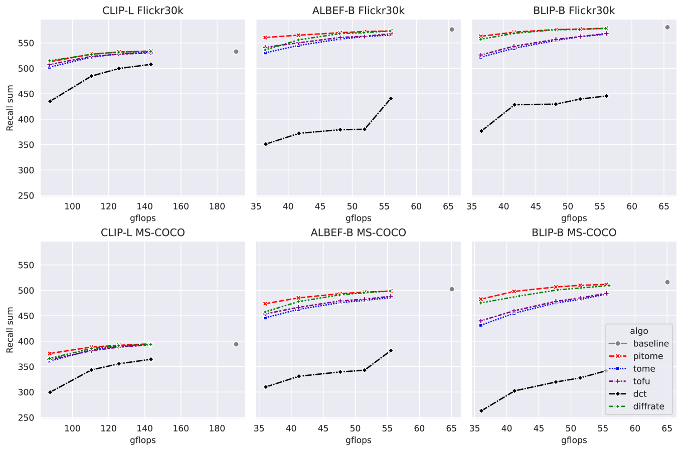
We evaluate PiToMe on the image-text retrieval task using three different backbone models CLIP [56], ALBEF [57], and BLIP [58] on two frequently used Flickr30k [59] and MSCOCO [60] datasets. Our experiment is benchmarked using $recall @ k$ [61], where a higher $recall @ k$ indicates the model’s effectiveness in retrieval. In Figure 3, we benchmarked PiToMe against other SOTA merging or pruning-based methods such as ToMe [15], ToFu [16], DiffRate [19], and DCT [62] on off-the-shelf setting when varying amount of merged tokens at each layer. Given the same FLOPS, it is clear that PiToMe consistently outperforms previous compression algorithms across all backbones. The performance gap increases as we decrease the percentage $r$ of tokens retained in each layer. The same behavior remains consistent in Table 2, where we set $r = 0.925$ and retrain pre-trained checkpoints of BLIP and CLIP. For more details about the training method, please refer to Li et al. [58].

In Table 2, we compare PiToMe using compression ratios of $r \in {0.95, 0.975}$ on BLIP and BLIP-2 against other advanced architectures such as ViLT [63], LightningDOT [64], UNITER [65], METER [66], CLIP-L [67], and ALBEF [68]. The results show that PiToMe consistently surpasses those architectures by a significant margin. Moreover, the performance drop on the base BLIP/BLIP-2 is minimal while achieving substantial reductions in memory footprint and rerank times—nearly halving for BLIP and tripling for BLIP-2. Additionally, the speedup can further improve with increased batch and model sizes.

4.2 Visual Question Answering (VQA) with Large Vision-Language Models

This experiment focuses on assessing the off-the-shelf performance of large vision-language models like LLaVa [2]. We extensively conduct experiments across six VQA datasets: VQA-v2 [69], GQA [70] (academic questions), VizWiz [71] (visually impaired individuals), ScienceQA [72] (zero-shot scientific question answering), TextVQA [73] (text-rich VQA tasks), and MME-Perception [74] (visual perception with yes/no question). More details on the number of samples in each dataset are in the Appendix. All experiments are conducted using LLAVA-1.5 7B and LLAVA-1.5 13B with the $lmms_eval$ library [75] provided by the LMMs-Lab team.

Table 1: Image-Text Retrieval comparison. PiToMe without training are in blue, and with training in gray. PiToMe achieves SOTA while saving

36 % - 56 %

in FLOPS and speeding up by

\times 1.4

to

\times 1.6

compared to the base models.

Datasets	Methods	$𝐑𝐭 @ 1$ $↑$	$𝐑𝐢 @ 1$ $↑$	ZS Retrieval $R s u m$ $↑$	Reranked $R s u m$ $↑$	ViT FLOPS $↓$	Total FLOPS $↓$	ZS Retrieval Time $↓$	Total Time $↓$
Flickr30k	ViLT	83.50	64.40	490.60	525.70	-	55.90	-	-
	LightingDOT	83.90	69.90	532.26	-	-	-	-	-
	UNITER	92.87	83.73	521.90	542.80	-	949.9	-	-
	METER	94.30	82.22	560.54	570.72	-	-	-	-
	CLIP-L	92.90	81.34	568.23	-	80.85	-	25s	-
	ALBEF	94.91	85.32	564.58	575.00	55.14	65.54	16s	58s
	${PiToMe}_{r = 0.95}^{BLIP}$	95.72	86.32	567.58	577.81	38.55	47.65	13s	56s
	${PiToMe}_{r = 0.95}^{BLIP}$	96.61	87.18	569.98	579.35	38.55	47.65	13s	56s
	BLIP	96.86	87.48	572.24	580.76	55.14	65.54	16s	1m17s
	${PiToMe}_{r = 0.95}^{BLIP2}$	96.83	87.84	566.25	580.77	296.93	390.77	45s	1m21s
	${PiToMe}_{r = 0.975}^{BLIP2}$	97.55	89.04	572.81	583.72	434.50	564.78	1m5s	1m54s
	BLIP2	97.61	89.79	572.72	584.76	678.45	900.77	1m37s	3m15s
MS-COCO	ViLT	61.50	42.70	420.20	439.20	-	55.90	-	-
	CLIP-L	70.78	53.79	478.18	-	80.85	-	2m10s	-
	METER	76.16	57.08	-	495.95	-	-	-	-
	ALBEF	76.94	60.24	478.39	500.44	55.14	65.54	43s	5m29s
	${PiToMe}_{r = 0.95}^{BLIP}$	79.46	62.50	485.99	506.65	38.85	47.65	51s	4m30s
	${PiToMe}_{r = 0.95}^{BLIP}$	80.44	63.91	493.33	512.66	38.85	47.65	51s	4m30s
	BLIP	81.82	64.36	494.34	516.03	55.14	65.54	1m3s	7m10s
	${PiToMe}_{r = 0.95}^{BLIP-2}$	82.29	65.54	494.92	518.44	296.93	390.77	3m33s	6m34s
	${PiToMe}_{r = 0.975}^{BLIP-2}$	84.12	67.37	504.95	527.06	434.50	564.78	5m13s	9m24s
	BLIP-2	85.32	68.26	507.46	528.63	678.45	900.77	7m52s	16m12s

Table 2: Retrained Image-Text Retrieval comparison when retraining from scratch on CLIP and BLIP backbones.

R k = R k @ 1 + R k @ 5 + R k @ 10, k \in {t, i}

,

Models	Algo.	$𝐑𝐭 ↑$	$𝐑𝐢 ↑$	GFLOPS $↑$	Eval Speed $↑$	Train Speed $↑$
${CLIP}_{Flickr}$	Baseline	291.80	275.52	x1.00	x1.00	x1.00
	ToMe	287.30	270.52	x2.10	x1.39	x1.79
	ToFu	288.32	269.68	x2.10	x1.39	x1.76
	DCT	279.70	258.24	x2.10	x1.30	x1.37
	DiffRate	289.33	266.45	x2.10	x1.39	x1.78
	PiToMe	291.50	270.94	x2.10	x1.39	x1.78
${BLIP}_{FLickr}$	Baseline	296.70	284.06	x1.00	x1.00	x1.00
	ToMe	294.80	280.64	x1.57	x1.66	x1.60
	ToFu	296.46	281.04	x1.57	x1.65	x1.59
	DCT	291.79	275.22	x1.57	x1.61	x1.45
	DiffRate	292.77	279.46	x1.57	x1.65	x1.59
	PiToMe	296.00	282.36	x1.57	x1.66	x1.59
${CLIP}_{coco}$	Baseline	256.30	222.21	x1.00	x1.00	x1.00
	ToMe	248.64	215.03	x2.10	x1.38	x1.79
	ToFu	248.99	216.56	x2.10	x1.39	x1.79
	DCT	240.04	211.28	x2.10	x1.34	x1.37
	DiffRate	248.87	215.45	x2.10	x1.39	x1.79
	PiToMe	250.70	217.01	x2.10	x1.39	x1.79
${BLIP}_{coco}$	Baseline	273.72	241.30	x1.00	x1.00	x1.00
	ToMe	266.86	234.67	x1.57	x1.90	x1.85
	ToFu	266.18	233.87	x1.57	x1.90	x1.85
	DCT	264.38	230.19	x1.57	x1.86	x1.78
	DiffRate	265.45	235.11	x1.57	x1.84	x1.85
	PiToMe	268.42	236.25	x1.57	x1.88	x1.85

Let $L$ denote the number of layers in the CLIP encoder and $N$ the number of visually encoded tokens. In our experiment, we apply PiToMe to the ViT vision encoder of LLAVA, retaining only $r$ percent of tokens in each layer. This results in $r^{L} N$ tokens being fed into the LLM, significantly enhancing inference speed. We used LLaVA-1.5-7B and LLaVA-1.5-13B checkpoints to run off-the-shelf settings. Tables 4 and 4, along with Figure 4, illustrate that the PiToMe algorithm consistently achieves superior performance compared to other merging and pruning methods, as well as existing SOTA models such as BLIP-2 [76], InstructBLIP [77], IDEFICS-9B/80B [78], with inference time nearly halved. Remarkably, in some datasets like VisWiz and ScienceQA, the compressed model even surpasses the baseline model. We contend that this improvement stems from the merging of less significant tokens in PiToMe, potentially enhancing the robustness of the language model (LLM).

4.3 Image Classification on Imagenet-1k

In this task, we employed five ViT backbones of varying sizes—tiny (ViT-T), small (ViT-S), base (ViT-B), large (ViT-L), and huge (ViT-H) - which are pre-trained using either MAE [79] or DEIT [80] styles. These backbones were utilized to assess both off-the-shelf and retrained performance. All experiments were conducted on the ImageNet-1k dataset, which is a subset of ImageNet [81] containing labeled images spanning 1000 categories.

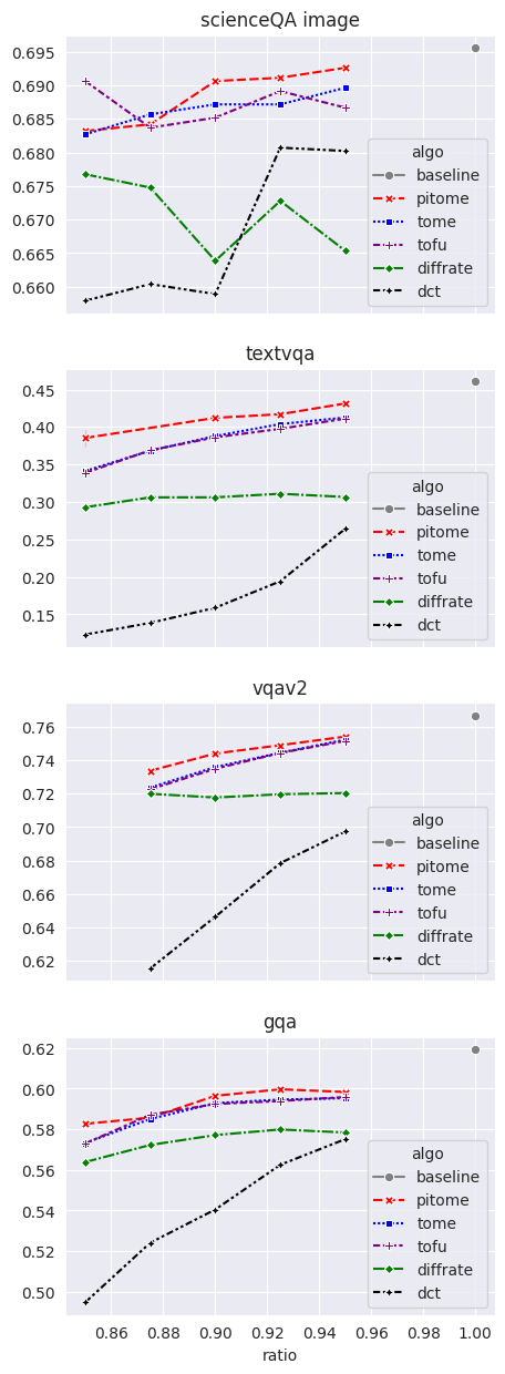
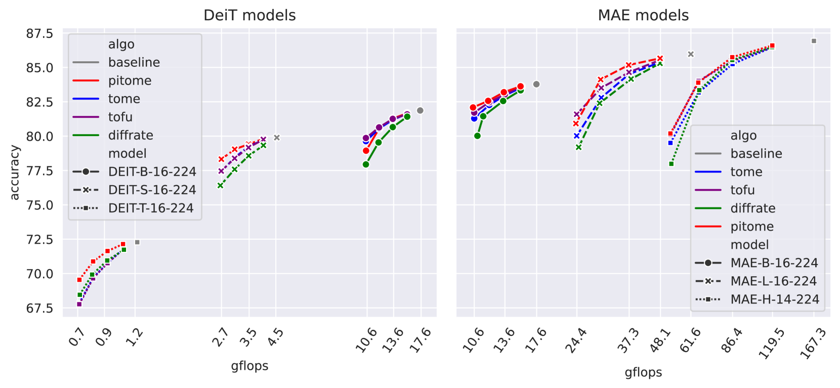
Table 5 and Figure 5 present our experimental results, comparing PiToMe with recent works, including SOTA efficient transformers such as Swin-B [82], CSWin-B [82], MViT-B/L [83], MAE [79], and other token merging/pruning methods [84, 85, 41]. We observe that PiToMe maintains high accuracy with an average performance drop of only $0.5 %$ after reducing up to $44 %$ of FLOPS (MAE-H), showcasing superior performance with comparable throughput. It is important to note that dynamic pruning-based methods such as A-ViT [85], Dynamic ViT [84], and SP-ViT [13] do not accelerate training speed due to using additional masks for padding tokens into a same dimension. On the retraining settings, we note that models compressed by PiToMe also surpass merging/pruning methods by a large margin and approach the performance of the original models.

4.4 Text Classification

While previous studies have focused on benchmarking BSM-based algorithms within the vision or vision-language domain, we also extend experiments to the text domain, where input sequence lengths vary by sample. Specifically, we apply compression algorithms to the first three layers of the BERT model [86], reducing the number of tokens by $20 %$ in each layer. Our experiments utilize the SST-2 dataset [87] with an average sequence length of 23.2 tokens and the IMDb dataset [88] with an average sequence length of 292.2 tokens.

As demonstrated in Table 6 and Figure 11 (Appendix), our findings indicate that PiToMe performs better than other BSM-based baselines. Additionally, after retraining, the compressed BERT models achieve competitive records while significantly accelerating training speed compared to previous pruning methods such as PowER-BERT [89], Fisher [90], and LTP [91], as well as BERT-based efficient models like DistilBERT [92] and ALBERT [93]. Notably, we observe only a $0.4 %$ performance drop on the IMDb dataset and even surpass the original BERT model by $0.3 %$ on the SST-2 dataset. For detailed empirical results on this task, please refer to Appendix D.

4.5 PiToMe Ablation Studies

Contributions of energy scores and related factors. To assess the performance of the components used in PiToMe, we conduct the following settings: (i) PiToMe without protecting important tokens by our energy in Step 2, i.e., using odd and even indices in sorted energy score array as two sets in BSM; (ii) PiToMe where the merging process in Step 3 conducted on two randomly sets $𝒜, ℬ$ as baselines [15, 16] instead of leveraging ordered in sorted energy vectors $𝐄 (.)$ ; (iii) PiToMe without using our proposed energy score as in Eq(4) but utilizing other indicators like attention scores from the $[CLS]$ (PiToMe w cls attn) token [19] or mean of attention scores; (iv) PiToMe using a fixed of $k$ removed token at each layer as ToMe [15] rather than a reducing ratio of $r$ as our configuration.

We run experiments on image-text retrieval and text classification tasks, reporting the results in Table 7 for (i) and (ii), and in Figure 6 for (iii) and (iv). The results demonstrate that all factors contribute to the performance of PiToMe, with energy-based operations playing a particularly significant role. Additionally, reducing tokens with a ratio $r$ effectively eliminates redundant tokens in early layers while preserving informative ones in later layers.

Margin $m$ and $α$ hyper-parameters. To validate the roles of these parameters in our energy score function in Eq.(4), we conduct ablation studies on image-text retrieval task with (v) adaptive margin $m$ compared with a fixed value $m \in {0.9, 0.45, 0.0, - 1.0}$ when varying the ratio $r$ and (vi) given a fixed value of $r$ , changing the smooth constant value $α$ in $α (\exp (x - m) - 1)$ with $x < m$ . Results for these settings are summarized in Figure 7 and Table 8, respectively. We observe that while models with fixed tend to have the accuracy drop sharply when it is lower than some threshold, the adaptive margins achieve the best results across cases. We hypothesize that as the token space becomes sparser in deeper layers, PiToMe’s fixed $m$ approach likely assigns the same energy score to all tokens, making it difficult to isolate and protect tokens during merging. Table 8 also shows that $α = 1.0$ is the best choice across margin values.

Further details, including additional ablation study results, visualizations (output merging, open-chat with LLaVa), and extra PiToMe experiments, are provided in the Appendix.

Table 7: Impact of different settings in Steps 2 and 3.

Settings	Image-Text Retrieval		Text CLS.
Settings	ratio $r$	$R s u m$	ratio $r$	acc
PiToMe w/o protecting tokens in step 2	0.925	568.9	0.6	86.99
	0.95	575.3	0.7	89.97
	0.975	578.2	0.8	91.67
PiToMe using random split in step 3	0.925	567.9	0.6	87.17
	0.95	574.7	0.7	90.34
	0.975	578.4	0.8	91.73
PiToMe	0.925	573.4	0.6	89.20
	0.95	577.8	0.7	91.47
	0.975	580.1	0.8	93.26

Table 8: Impact of the constant

α

on the image-text retrieval task. Results are in recall sum; higher is better.

ration $r$	$α = 1.0$	$α = 0.5$	$α = 0 .$
0.85	519.98	518.66	515.90
0.875	545.90	544.22	542.54
0.90	562.82	562.42	561.92
0.925	571.88	571.10	570.62
0.95	577.50	577.43	577.40
0.975	580.24	579.82	579.76

Figure 6: Ablation studies of PiToMe.

Figure 7: Ablation studies on adaptive margin

m

.

5 Conclusion

This paper introduces PiToMe, a novel algorithm that employs energy concepts to protect informative tokens during the token merging process. Our algorithm matches the efficiency of heuristic merging methods while maintaining a theoretical connection to the spectral properties of the input token space. In experiments on image classification, image-text retrieval, and VQA with LLaVA-1.5 7B/13B, PiToMe consistently outperforms recent token merging and pruning methods, given the equivalent runtime and memory usage.

Limitations and Future Works Although our focus has been on tasks using ViT encoders for a variety of applications, we believe it is important to extend PiToMe to generative tasks such as image generation (e.g., stable diffusion) or segmentation. This extension, however, necessitates the development of an unmerge mechanism in the decoder, which remains an open question. Additionally, our energy score relies on a fully connected graph of input tokens, which can increase complexity as the input size grows. Constructing sparse graphs, therefore, might be beneficial for scaling in more challenging settings. Finally, designing a differentiable learning mechanism to optimize the reducing rate $r$ for token merging could enhance robustness and versatility across different downstream tasks.

Acknowledgment

The authors thank the International Max Planck Research School for Intelligent Systems (IMPRS-IS) for supporting Duy M. H. Nguyen. Duy M. H. Nguyen and Daniel Sonntag are also supported by the XAINES project (BMBF, 01IW20005), No-IDLE project (BMBF, 01IW23002), and the Endowed Chair of Applied Artificial Intelligence, Oldenburg University. Hoai-Chau Tran acknowledges the support from the AISIA Extensive Research Assistant Program 2023 (Batch 1) during this work and DFKI for supporting computing resources. TrungTin Nguyen acknowledges support from the Australian Research Council grant DP230100905. Ngan Le acknowledges funding support from the U.S. National Science Foundation (NSF) under Award No. OIA-1946391 and NSF EFRI BRAID 2223793. Binh T. Nguyen wants to thank the University of Science, Vietnam National University in Ho Chi Minh City for their support. Mathias Niepert acknowledges funding by Deutsche Forschungsgemeinschaft (DFG, German Research Foundation) under Germany’s Excellence Strategy - EXC and support by the Stuttgart Center for Simulation Science (SimTech).

References

Dosovitskiy et al. [2020] Alexey Dosovitskiy, Lucas Beyer, Alexander Kolesnikov, Dirk Weissenborn, Xiaohua Zhai, Thomas Unterthiner, Mostafa Dehghani, Matthias Minderer, Georg Heigold, Sylvain Gelly, Jakob Uszkoreit, and Neil Houlsby. An image is worth 16x16 words: Transformers for image recognition at scale, 2020. ↩ a
Liu et al. [2024] Haotian Liu, Chunyuan Li, Qingyang Wu, and Yong Jae Lee. Visual instruction tuning. Advances in neural information processing systems, 36, 2024. ↩ a b
MH Nguyen et al. [2024] Duy MH Nguyen, Hoang Nguyen, Nghiem Diep, Tan Ngoc Pham, Tri Cao, Binh Nguyen, Paul Swoboda, Nhat Ho, Shadi Albarqouni, Pengtao Xie, et al. Lvm-med: Learning large-scale self-supervised vision models for medical imaging via second-order graph matching. Advances in Neural Information Processing Systems, 36, 2024. ↩ a
Kirillov et al. [2023] Alexander Kirillov, Eric Mintun, Nikhila Ravi, Hanzi Mao, Chloe Rolland, Laura Gustafson, Tete Xiao, Spencer Whitehead, Alexander C Berg, Wan-Yen Lo, et al. Segment anything. In Proceedings of the IEEE/CVF International Conference on Computer Vision, pages 4015–4026, 2023. ↩ a
Liu et al. [2022] Ze Liu, Jia Ning, Yue Cao, Yixuan Wei, Zheng Zhang, Stephen Lin, and Han Hu. Video swin transformer. In Proceedings of the IEEE/CVF conference on computer vision and pattern recognition, pages 3202–3211, 2022. ↩ a b
Dehghani et al. [2023] Mostafa Dehghani, Josip Djolonga, Basil Mustafa, Piotr Padlewski, Jonathan Heek, Justin Gilmer, Andreas Peter Steiner, Mathilde Caron, Robert Geirhos, Ibrahim Alabdulmohsin, et al. Scaling vision transformers to 22 billion parameters. In International Conference on Machine Learning, pages 7480–7512. PMLR, 2023. ↩ a
Katharopoulos et al. [2020] Angelos Katharopoulos, Apoorv Vyas, Nikolaos Pappas, and François Fleuret. Transformers are rnns: Fast autoregressive transformers with linear attention. In International conference on machine learning, pages 5156–5165. PMLR, 2020. ↩ a
Bolya et al. [2022] Daniel Bolya, Cheng-Yang Fu, Xiaoliang Dai, Peizhao Zhang, and Judy Hoffman. Hydra attention: Efficient attention with many heads. In European Conference on Computer Vision, pages 35–49. Springer, 2022. ↩ a b
Liu et al. [2021] Ze Liu, Yutong Lin, Yue Cao, Han Hu, Yixuan Wei, Zheng Zhang, Stephen Lin, and Baining Guo. Swin transformer: Hierarchical vision transformer using shifted windows. In Proceedings of the IEEE/CVF international conference on computer vision, pages 10012–10022, 2021. ↩ a b
Nguyen et al. [2023] Duy MH Nguyen, Hoang Nguyen, Truong TN Mai, Tri Cao, Binh T Nguyen, Nhat Ho, Paul Swoboda, Shadi Albarqouni, Pengtao Xie, and Daniel Sonntag. Joint self-supervised image-volume representation learning with intra-inter contrastive clustering. In Proceedings of the AAAI Conference on Artificial Intelligence, volume 37, pages 14426–14435, 2023. ↩ a b
Meng et al. [2022] Lingchen Meng, Hengduo Li, Bor-Chun Chen, Shiyi Lan, Zuxuan Wu, Yu-Gang Jiang, and Ser-Nam Lim. Adavit: Adaptive vision transformers for efficient image recognition. In Proceedings of the IEEE/CVF Conference on Computer Vision and Pattern Recognition, pages 12309–12318, 2022. ↩ a b
Michel et al. [2019] Paul Michel, Omer Levy, and Graham Neubig. Are sixteen heads really better than one? Advances in neural information processing systems, 32, 2019. ↩ a
Kong et al. [2022] Zhenglun Kong, Peiyan Dong, Xiaolong Ma, Xin Meng, Wei Niu, Mengshu Sun, Xuan Shen, Geng Yuan, Bin Ren, Hao Tang, et al. Spvit: Enabling faster vision transformers via latency-aware soft token pruning. In European conference on computer vision, pages 620–640. Springer, 2022. ↩ a b
Wei et al. [2023] Siyuan Wei, Tianzhu Ye, Shen Zhang, Yao Tang, and Jiajun Liang. Joint token pruning and squeezing towards more aggressive compression of vision transformers. In Proceedings of the IEEE/CVF Conference on Computer Vision and Pattern Recognition, pages 2092–2101, 2023. ↩ a
Bolya et al. [2023] Daniel Bolya, Cheng-Yang Fu, Xiaoliang Dai, Peizhao Zhang, Christoph Feichtenhofer, and Judy Hoffman. Token merging: Your ViT but faster. In International Conference on Learning Representations, 2023. ↩ a b c d e f g h i j k l m n o p q r s t
Kim et al. [2024] Minchul Kim, Shangqian Gao, Yen-Chang Hsu, Yilin Shen, and Hongxia Jin. Token fusion: Bridging the gap between token pruning and token merging. In Proceedings of the IEEE/CVF Winter Conference on Applications of Computer Vision, pages 1383–1392, 2024. ↩ a b c d e f g h i j k l m n o p
Cao et al. [2023] Qingqing Cao, Bhargavi Paranjape, and Hannaneh Hajishirzi. PuMer: Pruning and merging tokens for efficient vision language models. In Anna Rogers, Jordan Boyd-Graber, and Naoaki Okazaki, editors, Proceedings of the 61st Annual Meeting of the Association for Computational Linguistics (Volume 1: Long Papers), pages 12890–12903, Toronto, Canada, July 2023. Association for Computational Linguistics. doi: 10.18653/v1/2023.acl-long.721. ↩ a b c d
Bonnaerens and Dambre [2023] Maxim Bonnaerens and Joni Dambre. Learned thresholds token merging and pruning for vision transformers. Transactions on Machine Learning Research, 2023. ISSN 2835-8856. ↩ a b c
Chen et al. [2023] Mengzhao Chen, Wenqi Shao, Peng Xu, Mingbao Lin, Kaipeng Zhang, Fei Chao, Rongrong Ji, Yu Qiao, and Ping Luo. Diffrate : Differentiable compression rate for efficient vision transformers. In 2023 IEEE/CVF International Conference on Computer Vision (ICCV), pages 17118–17128, 2023. doi: 10.1109/ICCV51070.2023.01574. ↩ a b c d e f g h i j
Jiang et al. [2022] Chaoya Jiang, Haiyang Xu, Chenliang Li, Ming Yan, Wei Ye, Shikun Zhang, Bin Bi, and Songfang Huang. Trips: Efficient vision-and-language pre-training with text-relevant image patch selection. In Proceedings of the 2022 Conference on Empirical Methods in Natural Language Processing, pages 4084–4096, 2022. ↩ a
Park et al. [2023] Namuk Park, Wonjae Kim, Byeongho Heo, Taekyung Kim, and Sangdoo Yun. What do self-supervised vision transformers learn? International Conference on Learning Representations, 2023. ↩ a
Balakrishnan [2004] R Balakrishnan. The energy of a graph. Linear Algebra and its Applications, 387:287–295, 2004. ↩ a b
Gutman and Zhou [2006] Ivan Gutman and Bo Zhou. Laplacian energy of a graph. Linear Algebra and its applications, 414(1):29–37, 2006. ↩ a b
Loukas and Vandergheynst [2018a] Andreas Loukas and Pierre Vandergheynst. Spectrally approximating large graphs with smaller graphs. In International conference on machine learning, pages 3237–3246. PMLR, 2018a. ↩ a b c
Jin et al. [2020a] Yu Jin, Andreas Loukas, and Joseph JaJa. Graph coarsening with preserved spectral properties. In International Conference on Artificial Intelligence and Statistics, pages 4452–4462. PMLR, 2020a. ↩ a
Loukas [2019a] Andreas Loukas. Graph reduction with spectral and cut guarantees. Journal of Machine Learning Research, 20(116):1–42, 2019a. ↩ a
Wang et al. [2023a] Hongjie Wang, Bhishma Dedhia, and Niraj K Jha. Zero-tprune: Zero-shot token pruning through leveraging of the attention graph in pre-trained transformers. arXiv preprint arXiv:2305.17328, 2023a. ↩ a b
Shen et al. [2021] Zhuoran Shen, Mingyuan Zhang, Haiyu Zhao, Shuai Yi, and Hongsheng Li. Efficient attention: Attention with linear complexities. In Proceedings of the IEEE/CVF winter conference on applications of computer vision, pages 3531–3539, 2021. ↩ a
Dao et al. [2022] Tri Dao, Dan Fu, Stefano Ermon, Atri Rudra, and Christopher Ré. Flashattention: Fast and memory-efficient exact attention with io-awareness. Advances in Neural Information Processing Systems, 35:16344–16359, 2022. ↩ a
Daras et al. [2020] Giannis Daras, Nikita Kitaev, Augustus Odena, and Alexandros G Dimakis. Smyrf-efficient attention using asymmetric clustering. Advances in Neural Information Processing Systems, 33:6476–6489, 2020. ↩ a
Likhosherstov et al. [2021] Valerii Likhosherstov, Krzysztof M Choromanski, Jared Quincy Davis, Xingyou Song, and Adrian Weller. Sub-linear memory: How to make performers slim. Advances in Neural Information Processing Systems, 34:6707–6719, 2021. ↩ a
Ren et al. [2021] Hongyu Ren, Hanjun Dai, Zihang Dai, Mengjiao Yang, Jure Leskovec, Dale Schuurmans, and Bo Dai. Combiner: Full attention transformer with sparse computation cost. Advances in Neural Information Processing Systems, 34:22470–22482, 2021. ↩ a
Fayyaz et al. [2022] Mohsen Fayyaz, Soroush Abbasi Koohpayegani, Farnoush Rezaei Jafari, Sunando Sengupta, Hamid Reza Vaezi Joze, Eric Sommerlade, Hamed Pirsiavash, and Jürgen Gall. Adaptive token sampling for efficient vision transformers. In European Conference on Computer Vision, pages 396–414. Springer, 2022. ↩ a
Wang et al. [2023b] Wenhai Wang, Jifeng Dai, Zhe Chen, Zhenhang Huang, Zhiqi Li, Xizhou Zhu, Xiaowei Hu, Tong Lu, Lewei Lu, Hongsheng Li, et al. Internimage: Exploring large-scale vision foundation models with deformable convolutions. In Proceedings of the IEEE/CVF Conference on Computer Vision and Pattern Recognition, pages 14408–14419, 2023b. ↩ a
Rao et al. [2021a] Yongming Rao, Wenliang Zhao, Benlin Liu, Jiwen Lu, Jie Zhou, and Cho-Jui Hsieh. Dynamicvit: Efficient vision transformers with dynamic token sparsification. Advances in neural information processing systems, 34:13937–13949, 2021a. ↩ a
Touvron et al. [2021a] Hugo Touvron, Matthieu Cord, Matthijs Douze, Francisco Massa, Alexandre Sablayrolles, and Hervé Jégou. Training data-efficient image transformers & distillation through attention. In International conference on machine learning, pages 10347–10357. PMLR, 2021a. ↩ a
Goyal et al. [2020a] Saurabh Goyal, Anamitra Roy Choudhury, Saurabh Raje, Venkatesan Chakaravarthy, Yogish Sabharwal, and Ashish Verma. Power-bert: Accelerating bert inference via progressive word-vector elimination. In International Conference on Machine Learning, pages 3690–3699. PMLR, 2020a. ↩ a
Zhong et al. [2023] Qihuang Zhong, Liang Ding, Juhua Liu, Xuebo Liu, Min Zhang, Bo Du, and Dacheng Tao. Revisiting token dropping strategy in efficient bert pretraining. arXiv preprint arXiv:2305.15273, 2023. ↩ a
Yun et al. [2023] Jungmin Yun, Mihyeon Kim, and Youngbin Kim. Focus on the core: Efficient attention via pruned token compression for document classification. In The 2023 Conference on Empirical Methods in Natural Language Processing, 2023. ↩ a
Yin et al. [2022a] Hongxu Yin, Arash Vahdat, Jose M Alvarez, Arun Mallya, Jan Kautz, and Pavlo Molchanov. A-vit: Adaptive tokens for efficient vision transformer. In Proceedings of the IEEE/CVF Conference on Computer Vision and Pattern Recognition, pages 10809–10818, 2022a. ↩ a
Zhou et al. [2022] Yuxuan Zhou, Wangmeng Xiang, Chao Li, Biao Wang, Xihan Wei, Lei Zhang, Margret Keuper, and Xiansheng Hua. Sp-vit: Learning 2d spatial priors for vision transformers. In The 33rd British Machine Vision Conference, 2022. ↩ a b
Song et al. [2022] Zhuoran Song, Yihong Xu, Zhezhi He, Li Jiang, Naifeng Jing, and Xiaoyao Liang. Cp-vit: Cascade vision transformer pruning via progressive sparsity prediction. arXiv preprint arXiv:2203.04570, 2022. ↩ a
Bolya and Hoffman [2023] Daniel Bolya and Judy Hoffman. Token merging for fast stable diffusion. 2023 IEEE/CVF Conference on Computer Vision and Pattern Recognition Workshops (CVPRW), pages 4599–4603, 2023. ↩ a b
Shi et al. [2024] Dachuan Shi, Chaofan Tao, Anyi Rao, Zhendong Yang, Chun Yuan, and Jiaqi Wang. Crossget: Cross-guided ensemble of tokens for accelerating vision-language transformers. International Conference on Machine Learning, 2024. ↩ a b
Marin et al. [2023] Dmitrii Marin, Jen-Hao Rick Chang, Anurag Ranjan, Anish Prabhu, Mohammad Rastegari, and Oncel Tuzel. Token pooling in vision transformers for image classification. In Proceedings of the IEEE/CVF Winter Conference on Applications of Computer Vision, pages 12–21, 2023. ↩ a b
Bianchi et al. [2020] Filippo Maria Bianchi, Daniele Grattarola, and Cesare Alippi. Spectral clustering with graph neural networks for graph pooling. In International conference on machine learning, pages 874–883. PMLR, 2020. ↩ a b
Wu et al. [2022] Junran Wu, Xueyuan Chen, Ke Xu, and Shangzhe Li. Structural entropy guided graph hierarchical pooling. In International conference on machine learning, pages 24017–24030. PMLR, 2022. ↩ a b
Kumar et al. [2023] Manoj Kumar, Anurag Sharma, Shashwat Saxena, and Sandeep Kumar. Featured graph coarsening with similarity guarantees. In International Conference on Machine Learning, pages 17953–17975. PMLR, 2023. ↩ a
Clevert et al. [2016] Djork-Arné Clevert, Thomas Unterthiner, and Sepp Hochreiter. Fast and Accurate Deep Network Learning by Exponential Linear Units (ELUs). In ICLR 2016, 2016. ↩ a
Jin et al. [2020b] Yu Jin, Andreas Loukas, and Joseph JaJa. Graph Coarsening with Preserved Spectral Properties. In Silvia Chiappa and Roberto Calandra, editors, Proceedings of the Twenty Third International Conference on Artificial Intelligence and Statistics, volume 108 of Proceedings of Machine Learning Research, pages 4452–4462. PMLR, August 2020b. ↩ a b
Loukas [2019b] Andreas Loukas. Graph Reduction with Spectral and Cut Guarantees. Journal of Machine Learning Research, 20(116):1–42, 2019b. ↩ a b
Brissette et al. [2023] Christopher Brissette, Andy Huang, and George Slota. Spectrum Consistent Coarsening Approximates Edge Weights. SIAM Journal on Matrix Analysis and Applications, 44(3):1032–1046, 2023. doi: 10.1137/21M1458119. ↩ a
Loukas and Vandergheynst [2018b] Andreas Loukas and Pierre Vandergheynst. Spectrally Approximating Large Graphs with Smaller Graphs. In Jennifer Dy and Andreas Krause, editors, Proceedings of the 35th International Conference on Machine Learning, volume 80 of Proceedings of Machine Learning Research, pages 3237–3246. PMLR, July 2018b. ↩ a
Toivonen et al. [2011] Hannu Toivonen, Fang Zhou, Aleksi Hartikainen, and Atte Hinkka. Compression of weighted graphs. In Proceedings of the 17th ACM SIGKDD International Conference on Knowledge Discovery and Data Mining, KDD ’11, pages 965–973, New York, NY, USA, 2011. Association for Computing Machinery. ISBN 978-1-4503-0813-7. doi: 10.1145/2020408.2020566. ↩ a
Butler [2007] Steve Butler. Interlacing for weighted graphs using the normalized Laplacian. The Electronic Journal of Linear Algebra, 16:90–98, 2007. ↩ a
Radford et al. [2021a] Alec Radford, Jong Wook Kim, Chris Hallacy, Aditya Ramesh, Gabriel Goh, Sandhini Agarwal, Girish Sastry, Amanda Askell, Pamela Mishkin, Jack Clark, Gretchen Krueger, and Ilya Sutskever. Learning transferable visual models from natural language supervision. In Marina Meila and Tong Zhang, editors, Proceedings of the 38th International Conference on Machine Learning, volume 139 of Proceedings of Machine Learning Research, pages 8748–8763. PMLR, 18–24 Jul 2021a. ↩ a
Li et al. [2021a] Junnan Li, Ramprasaath R. Selvaraju, Akhilesh Deepak Gotmare, Shafiq Joty, Caiming Xiong, and Steven Hoi. Align before fuse: Vision and language representation learning with momentum distillation. In NeurIPS, 2021a. ↩ a
Li et al. [2022a] Junnan Li, Dongxu Li, Caiming Xiong, and Steven Hoi. BLIP: Bootstrapping language-image pre-training for unified vision-language understanding and generation. In Kamalika Chaudhuri, Stefanie Jegelka, Le Song, Csaba Szepesvari, Gang Niu, and Sivan Sabato, editors, Proceedings of the 39th International Conference on Machine Learning, volume 162 of Proceedings of Machine Learning Research, pages 12888–12900. PMLR, 17–23 Jul 2022a. ↩ a b
Plummer et al. [2015] Bryan A. Plummer, Liwei Wang, Chris M. Cervantes, Juan C. Caicedo, Julia Hockenmaier, and Svetlana Lazebnik. Flickr30k entities: Collecting region-to-phrase correspondences for richer image-to-sentence models. In Proceedings of the IEEE International Conference on Computer Vision (ICCV), December 2015. ↩ a b
Lin et al. [2014] Tsung-Yi Lin, Michael Maire, Serge Belongie, James Hays, Pietro Perona, Deva Ramanan, Piotr Dollár, and C. Lawrence Zitnick. Microsoft coco: Common objects in context. In David Fleet, Tomas Pajdla, Bernt Schiele, and Tinne Tuytelaars, editors, Computer Vision – ECCV 2014, pages 740–755, Cham, 2014. Springer International Publishing. ISBN 978-3-319-10602-1. ↩ a b
Cao et al. [2022] Min Cao, Shiping Li, Juntao Li, Liqiang Nie, and Min Zhang. Image-text retrieval: A survey on recent research and development. Thirty-First International Joint Conference on Artificial Intelligence (IJCAI)), 2022. ↩ a
He et al. [2023] Ziwei He, Meng Yang, Minwei Feng, Jingcheng Yin, Xinbing Wang, Jingwen Leng, and Zhouhan Lin. Fourier transformer: Fast long range modeling by removing sequence redundancy with fft operator. In Findings of the Association for Computational Linguistics: ACL 2023. Association for Computational Linguistics, 2023. doi: 10.18653/v1/2023.findings-acl.570. ↩ a
Kim et al. [2021] Wonjae Kim, Bokyung Son, and Ildoo Kim. Vilt: Vision-and-language transformer without convolution or region supervision. In International conference on machine learning, pages 5583–5594. PMLR, 2021. ↩ a
Sun et al. [2021] Siqi Sun, Yen-Chun Chen, Linjie Li, Shuohang Wang, Yuwei Fang, and Jingjing Liu. Lightningdot: Pre-training visual-semantic embeddings for real-time image-text retrieval. In Proceedings of the 2021 Conference of the North American Chapter of the Association for Computational Linguistics: Human Language Technologies, pages 982–997, 2021. ↩ a
Chen et al. [2020] Yen-Chun Chen, Linjie Li, Licheng Yu, Ahmed El Kholy, Faisal Ahmed, Zhe Gan, Yu Cheng, and Jingjing Liu. Uniter: Universal image-text representation learning. In European conference on computer vision, pages 104–120. Springer, 2020. ↩ a
Dou et al. [2022] Zi-Yi Dou, Yichong Xu, Zhe Gan, Jianfeng Wang, Shuohang Wang, Lijuan Wang, Chenguang Zhu, Pengchuan Zhang, Lu Yuan, Nanyun Peng, et al. An empirical study of training end-to-end vision-and-language transformers. In Proceedings of the IEEE/CVF Conference on Computer Vision and Pattern Recognition, pages 18166–18176, 2022. ↩ a
Radford et al. [2021b] Alec Radford, Jong Wook Kim, Chris Hallacy, Aditya Ramesh, Gabriel Goh, Sandhini Agarwal, Girish Sastry, Amanda Askell, Pamela Mishkin, Jack Clark, et al. Learning transferable visual models from natural language supervision. In International conference on machine learning, pages 8748–8763. PMLR, 2021b. ↩ a
Li et al. [2021b] Junnan Li, Ramprasaath Selvaraju, Akhilesh Gotmare, Shafiq Joty, Caiming Xiong, and Steven Chu Hong Hoi. Align before fuse: Vision and language representation learning with momentum distillation. Advances in neural information processing systems, 34:9694–9705, 2021b. ↩ a
Goyal et al. [2017] Yash Goyal, Tejas Khot, Douglas Summers-Stay, Dhruv Batra, and Devi Parikh. Making the V in VQA matter: Elevating the role of image understanding in Visual Question Answering. In Conference on Computer Vision and Pattern Recognition (CVPR), 2017. ↩ a b c
Hudson and Manning [2019] D. A. Hudson and C. D. Manning. Gqa: A new dataset for real-world visual reasoning and compositional question answering. In 2019 IEEE/CVF Conference on Computer Vision and Pattern Recognition (CVPR), pages 6693–6702, Los Alamitos, CA, USA, jun 2019. IEEE Computer Society. doi: 10.1109/CVPR.2019.00686. ↩ a b c
Gurari et al. [2018] Danna Gurari, Qing Li, Abigale J. Stangl, Anhong Guo, Chi Lin, Kristen Grauman, Jiebo Luo, and Jeffrey P. Bigham. Vizwiz grand challenge: Answering visual questions from blind people. In 2018 IEEE/CVF Conference on Computer Vision and Pattern Recognition, pages 3608–3617, 2018. doi: 10.1109/CVPR.2018.00380. ↩ a b c
Lu et al. [2022] Pan Lu, Swaroop Mishra, Tony Xia, Liang Qiu, Kai-Wei Chang, Song-Chun Zhu, Oyvind Tafjord, Peter Clark, and Ashwin Kalyan. Learn to explain: Multimodal reasoning via thought chains for science question answering. In The 36th Conference on Neural Information Processing Systems (NeurIPS), 2022. ↩ a b c
Singh et al. [2019] Amanpreet Singh, Vivek Natarajan, Meet Shah, Yu Jiang, Xinlei Chen, Dhruv Batra, Devi Parikh, and Marcus Rohrbach. Towards vqa models that can read. In 2019 IEEE/CVF Conference on Computer Vision and Pattern Recognition (CVPR), pages 8309–8318, 2019. doi: 10.1109/CVPR.2019.00851. ↩ a b c
Fu et al. [2023] Chaoyou Fu, Peixian Chen, Yunhang Shen, Yulei Qin, Mengdan Zhang, Xu Lin, Jinrui Yang, Xiawu Zheng, Ke Li, Xing Sun, Yunsheng Wu, and Rongrong Ji. Mme: A comprehensive evaluation benchmark for multimodal large language models. arXiv preprint arXiv:2306.13394, 2023. ↩ a b c
Li et al. [2024] Bo Li, Peiyuan Zhang, Kaichen Zhang, Fanyi Pu, Xinrun Du, Yuhao Dong, Haotian Liu, Yuanhan Zhang, Ge Zhang, Chunyuan Li, and Ziwei Liu. Lmms-eval: Accelerating the development of large multimoal models, March 2024. ↩ a
Li et al. [2023] Junnan Li, Dongxu Li, Silvio Savarese, and Steven Hoi. BLIP-2: Bootstrapping language-image pre-training with frozen image encoders and large language models. In Andreas Krause, Emma Brunskill, Kyunghyun Cho, Barbara Engelhardt, Sivan Sabato, and Jonathan Scarlett, editors, Proceedings of the 40th International Conference on Machine Learning, volume 202 of Proceedings of Machine Learning Research, pages 19730–19742. PMLR, 23–29 Jul 2023. ↩ a
Dai et al. [2024] Wenliang Dai, Junnan Li, Dongxu Li, Anthony Meng Huat Tiong, Junqi Zhao, Weisheng Wang, Boyang Li, Pascale N Fung, and Steven Hoi. Instructblip: Towards general-purpose vision-language models with instruction tuning. Advances in Neural Information Processing Systems, 36, 2024. ↩ a
IDEFICS [2023] IDEFICS. Introducing idefics: An open reproduction of state-of-the-art visual language model. https://huggingface.co/blog/idefics, 2023. Accessed: 2023-05-21. ↩ a
He et al. [2021] Kaiming He, Xinlei Chen, Saining Xie, Yanghao Li, Piotr Dollár, and Ross Girshick. Masked autoencoders are scalable vision learners. arXiv:2111.06377, 2021. ↩ a b
Touvron et al. [2021b] Hugo Touvron, Matthieu Cord, Matthijs Douze, Francisco Massa, Alexandre Sablayrolles, and Herve Jegou. Training data-efficient image transformers & distillation through attention. In International Conference on Machine Learning, volume 139, pages 10347–10357, July 2021b. ↩ a
Russakovsky et al. [2015] Olga Russakovsky, Jia Deng, Hao Su, Jonathan Krause, Sanjeev Satheesh, Sean Ma, Zhiheng Huang, Andrej Karpathy, Aditya Khosla, Michael Bernstein, Alexander C. Berg, and Li Fei-Fei. ImageNet Large Scale Visual Recognition Challenge. International Journal of Computer Vision (IJCV), 115(3):211–252, 2015. doi: 10.1007/s11263-015-0816-y. ↩ a b
Dong et al. [2021] Xiaoyi Dong, Jianmin Bao, Dongdong Chen, Weiming Zhang, Nenghai Yu, Lu Yuan, Dong Chen, and Baining Guo. Cswin transformer: A general vision transformer backbone with cross-shaped windows, 2021. ↩ a b
Li et al. [2022b] Yanghao Li, Chao-Yuan Wu, Haoqi Fan, Karttikeya Mangalam, Bo Xiong, Jitendra Malik, and Christoph Feichtenhofer. Mvitv2: Improved multiscale vision transformers for classification and detection. In CVPR, 2022b. ↩ a
Rao et al. [2021b] Yongming Rao, Wenliang Zhao, Benlin Liu, Jiwen Lu, Jie Zhou, and Cho-Jui Hsieh. Dynamicvit: Efficient vision transformers with dynamic token sparsification. In Advances in Neural Information Processing Systems (NeurIPS), 2021b. ↩ a b
Yin et al. [2022b] Hongxu Yin, Arash Vahdat, Jose Alvarez, Arun Mallya, Jan Kautz, and Pavlo Molchanov. A-ViT: Adaptive tokens for efficient vision transformer. In Proceedings of the IEEE/CVF Conference on Computer Vision and Pattern Recognition, 2022b. ↩ a b
Devlin et al. [2019] Jacob Devlin, Ming-Wei Chang, Kenton Lee, and Kristina Toutanova. Bert: Pre-training of deep bidirectional transformers for language understanding. Proceedings of naacL-HLT, 2019. ↩ a
Socher et al. [2013] Richard Socher, Alex Perelygin, Jean Wu, Jason Chuang, Christopher D Manning, Andrew Y Ng, and Christopher Potts. Recursive deep models for semantic compositionality over a sentiment treebank. In Proceedings of the 2013 conference on empirical methods in natural language processing, pages 1631–1642, 2013. ↩ a b
Maas et al. [2011] Andrew Maas, Raymond E Daly, Peter T Pham, Dan Huang, Andrew Y Ng, and Christopher Potts. Learning word vectors for sentiment analysis. In Proceedings of the 49th annual meeting of the association for computational linguistics: Human language technologies, pages 142–150, 2011. ↩ a b
Goyal et al. [2020b] Saurabh Goyal, Anamitra Roy Choudhury, Saurabh Raje, Venkatesan Chakaravarthy, Yogish Sabharwal, and Ashish Verma. Power-bert: Accelerating bert inference via progressive word-vector elimination. In International Conference on Machine Learning, pages 3690–3699. PMLR, 2020b. ↩ a
Kwon et al. [2022] Woosuk Kwon, Sehoon Kim, Michael W Mahoney, Joseph Hassoun, Kurt Keutzer, and Amir Gholami. A fast post-training pruning framework for transformers. Advances in Neural Information Processing Systems, 35:24101–24116, 2022. ↩ a
Kim et al. [2022] Sehoon Kim, Sheng Shen, David Thorsley, Amir Gholami, Woosuk Kwon, Joseph Hassoun, and Kurt Keutzer. Learned token pruning for transformers. In Proceedings of the 28th ACM SIGKDD Conference on Knowledge Discovery and Data Mining, pages 784–794, 2022. ↩ a
Sanh et al. [2019] Victor Sanh, Lysandre Debut, Julien Chaumond, and Thomas Wolf. Distilbert, a distilled version of bert: smaller, faster, cheaper and lighter. arXiv preprint arXiv:1910.01108, 2019. ↩ a
Lan et al. [2019] Zhenzhong Lan, Mingda Chen, Sebastian Goodman, Kevin Gimpel, Piyush Sharma, and Radu Soricut. Albert: A lite bert for self-supervised learning of language representations. arXiv preprint arXiv:1909.11942, 2019. ↩ a
Wolkowicz and Styan [1980] Henry Wolkowicz and George P. H. Styan. Bounds for eigenvalues using traces. Linear Algebra and its Applications, 29:471–506, 1980. ISSN 0024-3795. doi: https://doi.org/10.1016/0024-3795(80)90258-X. ↩ a
Weyl [1912] Hermann Weyl. Das asymptotische Verteilungsgesetz der Eigenwerte linearer partieller Differentialgleichungen (mit einer Anwendung auf die Theorie der Hohlraumstrahlung). Mathematische Annalen, 71(4):441–479, December 1912. ISSN 1432-1807. doi: 10.1007/BF01456804. ↩ a

Supplement to “Accelerating Transformers with Spectrum-Preserving Token Merging”

Figure 8: Token merging outputs can be seen as coarsened graph from an input graph.

Appendix A Datasets Descriptions

We present in Table 9 datasets used in our experiment. It is important to note that PiToMe was run off-the-shelf on large datasets in VQA tasks such as VQA-v2 with $447.8 k$ sample or GQQ with $12.5$ questions, validating generalization and robustness of our merging mechanism.

Table 9: Brief statistic of all datasets used in this paper.

Task	Name	Modality	No. Train	No. Test
Image-Text retrieval	Flickr30k [59]	Vision, Text	29k images, each with 5 captions	1k images, each with 5 captions
Image-Text retrieval	MS-COCO[60]	Vision, Text	approx 118k images, each with 5 captions	5k images, each with 5 captions
Visual Question Answering	VQA-v2[69]	Vision, Text	approx 443.7k questions	approx 447.8k questions
	GQA [70]	Vision, Text	approx 72k images with 943k questions	approx 10.2k images with 12.5k questions
	VisWiz [71]	Vision, Text	8k image and questions	approx 4.32k image and questions
	TextVQA[73]	Vision, Text	approx 28.4k images with 34.6k questions	approx 3.1k images with 4.2k questions
	MME [74]	Vision, Text	-	2375 images and questions
	ScienceQA[72]	Vision, Text	approx 4.11k image and questions	approx 2.11k image and questions
Text Classification	IMDb [88]	Text	25k movie reviews.	25k movie reviews.
Text Classification	SST-2 [87]	Text	67,349 sentences	872 sentences
Image Classification	Imagenet-1k[81]	Vision	Approximately approx 1.28 million images	50k images (50 images per class)

Appendix B PiToMe Algorithm

B.1 Pseudo-Code Implementation

The pseudo-code for our method is provided in Algorithm 1. Here E in line 3 is a vector that represents energy scores of all nodes calculated by the energy function 4. The final output is a $MERGE (.)$ function, which serves as a lambda function that can be applied to any matrix ${\hat{𝐗}}^{l}$ at the $l$ -th layer. The vector m is a vector that contains information about token sizes (i.e, the number of tokens being merged into each token).

Algorithm 1 PiToMe Algorithm

1:function pitome(

remain token ratio: r, input graph: 𝒢 (𝒱, ℰ)

) // Function to prepare for merging

2:

k \leftarrow N - N \cdot r

// Compute number of nodes to merge

3:

s \leftarrow argsort (𝐄, descending=True)

// Compute energy scores

4:

merge, protect \leftarrow s [: 2 \cdot k], s [2 \cdot k :]

// Identify mergeable and protected nodes

5:

n_{a}, n_{b} \leftarrow merge [: : 2], merge [1 : : 2]

// Split mergeable nodes

6:

ℰ_{m e r g e} \leftarrow ℰ [n_{a}] [n_{b}]

// Get edge weights of mergeable nodes

7:

n_{d s t} \leftarrow argmax (ℰ_{m e r g e})

// Find closest neighbors

8: function Merge(X) // Function to perform merging

9:

X_{p r o t e c t e d} \leftarrow X [protect, :]

// Extract protected tokens

10:

X_{𝒜}, X_{ℬ} \leftarrow X [n_{a}, :], X [n_{b}, :]

// Extract tokens in set

𝒜

and

ℬ

11:

X_{𝒜}, X_{ℬ} \leftarrow X_{𝒜} \times m [n_{a}], X_{ℬ} \times m [n_{b}]

// Weighted average

12:

X_{ℬ} \leftarrow X_{ℬ} . scatter_reduce (n_{d s t}, X_{𝒜}, mode = "sum")

// Merge tokens

13:

X_{ℬ} \leftarrow X_{ℬ} / m_{ℬ} . scatter_reduce (n_{d s t}, m_{𝒜}, mode = "sum")

// Weighted average

14: return

cat (X_{p r o t e c t e d}, X_{ℬ})

// Concatenate and return merged tokens

15: return MERGE // Return merging lambda function

B.2 PiToMe Complexity Analysis

In algorithm 1, in line $3$ , the weighted graph is constructed through matrix multiplication, leading to a complexity of $𝒪 (N^{2} h)$ , where $h$ is the dimension of input vectors. Next, the computed energy scores are sorted, which have the complexity of $𝒪 (N \log (N))$ . Lastly, in line $7$ , the max operator for selecting the merge destination and the lambda $M E R G E$ function, which performs tensor operations based on computed indices, lead to linear complexity. Combining these aspects, the overall time complexity of the PiToMe function can be approximated as $𝒪 (N^{2} h)$ , considering the dominant factors contributing to computational cost. However, actual performance may vary depending on the specific PyTorch version and hardware utilization, with optimizations potentially altering these estimates.

In the BSM algorithms used by ToMe, after the bipartition of tokens into two sets $𝒜$ and $ℬ$ using odd and even indices, each set has $N / 2$ tokens, it also requires calculating a similarity matrix between tokens in these two sets. This operation also has the complexity of $𝒪 (N^{2} h)$ . The similarity matrix is then sorted to get the top $k$ tokens in set $𝒜$ with the highest similarity score used for merging, this operation also has the time complexity of $𝒪 (N \log (N))$ , and the merging procedure is the same as our PiToMe algorithm. So basically when compared to BSM, our algorithms have the same time complexity of $𝒪 (N^{2} h)$ , although in practice the speed of ToMe is a little bit faster than PiToMe (a few milliseconds), but our algorithms give a much better trade-off between speed and accuracy. For more details about the BSM algorithms please refer to the ToMe paper[15].

B.3 Model complexity analysis

In a standard Transformer layer, we have the time and space complexity to be $𝒪 (N^{2} h + N h^{2})$ and $𝒪 (N^{2} + N h)$ . In each layer $i t h$ of the model, we compress the number of tokens down to $r N$ using PiToMe algorithms with the complexity of $𝒪 ({(r^{i - 1} N)}^{2} h)$ , so the layer $i$ will enjoy the time and space complexity of $𝒪 ({(r^{i - 1} N)}^{2} h + r^{i} N h^{2} + {(r^{i - 1} N)}^{2} h)$ and $𝒪 ({(r^{i - 1} N)}^{2} + r^{i} N h)$ resp.Vision language models like LLaVA directly use output tokens from ViT encoders. Let $l$ be the number of layers in the ViT encoder since we utilize PiToMe in each layer in the ViT encoder part; the LLM model will have the time and space complexity of $𝒪 ({(r^{l} N_{ViT} + N_{LLM})}^{2} h + (r^{l} N_{ViT} + N_{LLM}) h^{2})$ and $𝒪 ({(r^{l} N_{ViT} + N_{LLM})}^{2} + (r^{l} N_{ViT} + N_{LLM}) h)$ which boosts the inference speed and saves a high amount of memory usage. The speedup could get even more impressive when used with higher batch size and image size. This also applies to models that use cross-attention modules for image text matching like BLIP and ALBEF, in which most of the computation expense comes from tokens encoded by the ViT model, the time and space complexity for the cross attention layers are $𝒪 (r^{l} N_{vision} N_{text} h + N_{text} h^{2})$ and $𝒪 (r^{l} N_{vision} N_{text} + N_{text} h)$ resp.

Appendix C Performance of ToMe with Different Token Merging Schedules

In the original ToMe paper, the authors proposed a merging schedule that involves reducing tokens in each layer by a fixed $k$ tokens per layer. However, as illustrated in Figure 6, we showed that this merging schedule is suboptimal for off-the-shell performance, and this section provides empirical results to confirm this claim.

In this experiment, we exclusively compare two versions of the BSM algorithms utilized in the ToMe paper: one that preserves a percentage $r$ of tokens in each layer and another that reduces a fixed $k$ tokens in each layer. However, for a more comprehensive comparison, we extensively apply these algorithms across 6 ViT backbones (DeiT-T, DeiT-S, DeiT-B, MAE-B, MAE-L, MAE-H) for image classification tasks using the Imagenet-1k dataset, as well as across 4 backbones for image-text retrieval tasks (CLIP-B, CLIP-L, BLIP, BLIP2) on FLickr30k and MSCOCO dataset.

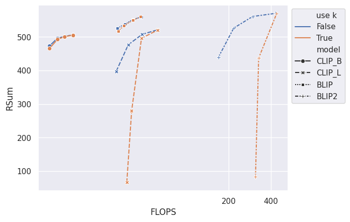
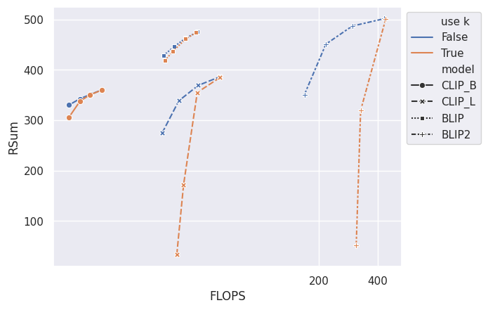
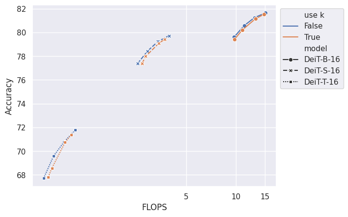
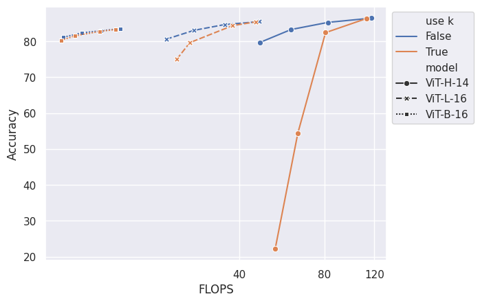
From Figures 10, 10, 9, and 9, it is evident that, given the same FLOPS, the BSM version that uses the remaining percent $r$ shows a clear advantage, outperforming the original schedule by a large margin. This gap becomes even more pronounced when benchmarked on large models like MAE-L, MAE-H, and BLIP-2. During the experiment, we also observed that models compressed using the ratio $r$ tend to run a little faster since a large number of tokens are removed in earlier layers.

Appendix D Additional Experiments on Text Classification Task.

This section comprehensively assesses the performance of PiToMe against other baseline algorithms for sentiment text classification tasks. We conducted this experiment using the IMDb and SST-2, applying the compression algorithms to the first three layers of the model. To ensure consistency in our experimental results, we used two different backbones: BERT with 12 layers and DistilBERT with 6 layers. Since we only compress the first three layers, in addition to the baselines previously used throughout this paper, we introduced two additional baselines: ToFu-p and ToFu-m. ToFu-p uses BSM to prune tokens instead of merging them, while ToFu-m represents the original ToFu algorithm without pruning.

Table 10: Performance of PiToMe versus baselines algorithms when training BERT and DistiledBERT when retrained from scratch.

Dataset

Model

Compress method

r = 0.8

r = 0.75

r = 0.7

accuracy

flops

eval speed

train speed

accuracy

flops

eval speed

train speed

accuracy

flops

eval speed

train speed

SST-2

BERT

ToMe

91.25 (-0.20)

x1.88

x1.14

x1.40

89.12 (-2.33)

x2.27

x1.22

x1.56

88.00 (-3.45)

x2.72

x1.30

x1.68

ToFu

89.82 (-1.83)

x1.88

x1.15

x1.40

88.64 (-2.81)

x2.27

x1.22

x1.56

87.22 (-4.23)

x2.72

x1.29

x1.68

DCT

90.66 (-0.79)

x1.81

x1.05

x1.12

89.31 (-2.14)

x2.13

x1.12

x1.43

87.76 (-3.69)

x2.72

x1.19

x1.61

DiffRate

89.72 (-1.73)

x1.88

x1.14

x1.40

87.96 (-3.49)

x2.27

x1.21

x1.55

87.64 (-3.81)

x2.72

x1.22

x1.68

PiToMe

91.72 (+0.27)

x1.88

x1.19

x1.39

90.28 (-1.17)

x2.27

x1.23

x1.55

88.67 (-2.78)

x2.72

x1.25

x1.65

DistiledBERT

ToMe

89.64 (-1.74)

x1.61

x1.01

x1.28

88.56 (-2.82)

x1.88

x1.03

x1.35

88.64 (-2.74)

x2.26

x1.07

x1.46

ToFu

89.92 (-1.46)

x1.61

x1.02

x1.27

88.85 (-2.53)

x1.88

x1.04

x1.35

88.76 (-2.62)

x2.26

x1.07

x1.46

DCT

89.59 (-1.79)

x1.51

x0.95

x1.16

88.08 (-3.30)

x1.61

x1.00

x1.22

87.70 (-3.68)

x1.88

x1.02

x1.32

DiffRate

89.65 (-1.73)

x1.61

x1.01

x1.26

89.05 (-2.33)

x1.88

x1.02

x1.33

87.88 (-3.50)

x2.26

x1.07

x1.42

PiToMe

90.31 (-1.07)

x1.61

x1.02

x1.25

89.28 (-2.10)

x1.88

x1.05

x1.34

88.89 (-2.49)

x2.26

x1.10

x1.41

IMDb

BERT

ToMe

93.25 (-0.75)

x1.91

x1.68

x1.86

93.01 (-0.99)

x2.30

x1.88

x2.06

92.33 (-1.67)

x2.77

x2.10

x2.36

ToFu

93.36 (-0.64)

x1.92

x1.68

x1.86

92.99 (-1.01)

x2.30

x1.89

x2.06

92.34 (-1.66)

x2.77

x2.09

x2.34

DCT

92.39 (-1.61)

x1.90

x1.60

x1.79

92.22 (-1.78)

x2.30

x1.75

x1.94

91.31 (-2.69)

x2.77

x1.97

x2.25

DiffRate

92.96 (-1.04)

x1.91

x1.68

x1.86

92.53 (-1.47)

x2.30

x1.86

x2.03

92.10 (-1.90)

x2.77

x2.08

x2.33

PiToMe

93.52 (-0.48)

x1.91

x1.66

x1.84

93.27 (-0.73)

x2.30

x1.84

x2.01

92.74 (-1.26)

x2.77

x2.08

x2.31

DistiledBERT

ToMe

92.45 (-0.55)

x1.83

x1.47

x1.57

92.34 (-0.66)

x2.15

x1.57

x1.64

91.86 (-1.14)

x2.53

x1.69

x1.86

ToFu

92.55 (-0.45)

x1.83

x1.47

x1.57

92.33 (-0.67)

x2.15

x1.57

x1.64

91.91 (-1.09)

x2.53

x1.69

x1.85

DCT

92.38 (-0.62)

x1.61

x1.39

x1.50

91.87 (-1.13)

x1.79

x1.48

x1.62

91.69 (-1.31)

x2.19

x1.56

x1.77

DiffRate

92.43 (-0.57)

x1.83

x1.44

x1.55

92.16 (-0.84)

x2.15

x1.57

x1.62

91.78 (-1.22)

x2.53

x1.63

x1.84

PiToMe

92.71 (-0.29)

x1.83

x1.43

x1.54

92.55 (-0.45)

x2.15

x1.54

x1.61

92.06 (-0.94)

x2.53

x1.62

x1.83

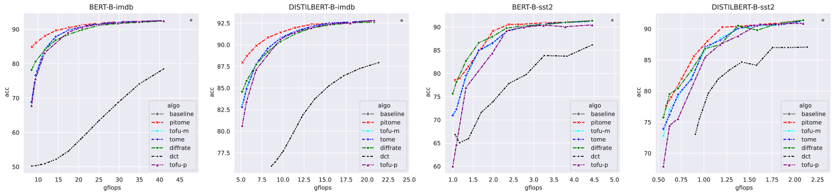
As demonstrated in Table 10 and Figure 11, our findings align with empirical results from previous tasks, indicating that PiToMe consistently achieves superior performance compared to other baselines. Particularly noteworthy is the performance on the IMDb dataset with a large context length, where even after reducing FLOPs by 80%, models compressed by PiToMe still maintain off-the-shelf accuracy above 85%, while other baseline algorithms see the off-the-shelf accuracy drop below 70%. Furthermore, Table 10 highlights that our algorithm can also facilitate better model learning compared to other methods, achieving high accuracy that closely approaches that of the original model.

Appendix E Proof of Theorem 1

E.1 Sketch of Proof

The proof sketch for Theorem 1 begins by defining coarsened and lifted versions of the original graph $𝒢$ (see Definitions 1 and 2) using the PiToMe and ToMe algorithms. The goal is to demonstrate that the spectral distance between $𝒢$ and its PiToMe-coarsened counterpart converges to zero, whereas the distance for ToMe remains bounded away from zero. The sketch proceeds by introducing Propositions 1, 2, and 3, which build toward the main result:

1.

Proposition 1 establishes upper bounds on the edge weight differences between merged nodes under the PiToMe and ToMe methods.
2.

Proposition 2 employs standard mild assumptions to relate the cosine similarity among nodes within clusters, demonstrating that the upper bound error $ϵ_{PiToMe}^{(s)}$ between the edge weights of merged nodes in PiToMe-coarsened graphs $𝒢_{PiToMe}^{(n)}$ converges to $0$ , whereas this property does not hold for the ToMe-coarsened graphs $𝒢_{ToMe}^{(n)}$ .
3.

Proposition 3 completes the sketch by bounding the spectral distances of the coarsened graphs in terms of the edge weight differences from the earlier Propositions 1 and 2.

Each proposition is proven in detail within the appendix sections following this sketch. Note that Theorem 1 immediately follows the following Propositions 1, 2, and 3, which are proved resp. in Sections E.2, E.3, and E.4.

Proposition 1.

Suppose the graphs $𝒢_{0}^{(s)}$ , $𝒢_{PiToMe}^{(s)}$ , and $𝒢_{ToMe}^{(s)}$ are coarsened from the original graph $𝒢$ by iteratively merging pairs of nodes $v_{a_{s}}$ and $v_{b_{s}}$ w.r.t. the true partition $𝒫_{0}^{(s)} = {𝒱_{0 i}^{(s)}}_{i \in [s]}$ , the PiToMe-partition $𝒫_{PiToMe}^{(s)} = {𝒱_{PiToMe i}^{(s)}}_{i \in [s]}$ , defined by PiToMe Algorithm 1, and the ToMe-partition [15, 16], $𝒫_{ToMe}^{(s)} = {𝒱_{ToMe i}^{(s)}}_{i \in [s]}$ , for $s = N, \dots, n + 1$ . We assume the following standard mild assumption:

(A2).

There exists a margin $m$ s.t.

$\cos (v_{a_{s}}, v_{b_{s}}) \geq m > \cos (v_{a_{s}}, v_{c_{s}}), \forall v_{a_{s}} \in 𝒱_{0 i}^{(s)}, \forall v_{b_{s}} \in 𝒱_{0 i}^{(s)}, \forall v_{c_{s}} \in 𝒱_{0 j}^{(s)}, \forall i \neq j \in [s] .$ (6)

Then, the edge weights of merged nodes from PiToMe Algorithm 1 and the ToMe-partition [15, 16] satisfy

{‖ 𝐖 [a_{s}, :] - 𝐖 [b_{s}, :] ‖}_{1} \leq ϵ^{(s)}

(7)

for some nonnegative upper bounds $ϵ^{(s)}$ , $s = N, N - 1, \dots, n + 1$ defined as follows:

ϵ^{(s)} = {\begin{matrix} 2 (1 - \cos (v_{a_{s}}, v_{b_{s}})) & if v_{a_{s}} \in 𝒱_{0 i}^{(s)}, v_{b_{s}} \in 𝒱_{0 i}^{(s)}, \forall i \in [s], \\ 3 (1 - β) & if v_{a_{s}} \in 𝒱_{0 i}^{(s)}, v_{b_{s}} \in 𝒱_{0 j}^{(s)}, i \neq j \in [s] . \end{matrix} .

(8)

Proposition 2.

We assume some standard mild assumptions:

(A1).

$𝔼 [\cos (v_{a_{s}}, v_{b_{s}})] \to 1, \forall v_{a_{s}} \in 𝒱_{0 i}^{(s)}, \forall v_{b_{s}} \in 𝒱_{0 i}^{(s)}, i \in [s]$ .
(A2).

There exists a margin $m$ s.t., $\cos (v_{a_{s}}, v_{b_{s}}) \geq m > \cos (v_{a_{s}}, v_{c_{s}}), \forall v_{a_{s}} \in 𝒱_{0 i}^{(s)}, \forall v_{b_{s}} \in 𝒱_{0 i}^{(s)}, \forall v_{c_{s}} \in 𝒱_{0 j}^{(s)}, \forall i \neq j \in [s]$ .
(A3).

There is an order of cardinality in the true partition, without loss of generality, we assume $N_{1}^{(s)} \geq N_{2}^{(s)} \geq \dots \geq N_{s}^{(s)}$ , where $N_{i}^{(s)} = | 𝒱_{0 i}^{(s)} |, \forall i \in [s]$ .

Here $𝔼 (\cdot)$ stands for the expectation of the random variables that define the random events $M_{a b}^{(s)} := {v_{a_{s}} \in 𝒱_{0 i}^{(s)}, v_{b_{s}} \in 𝒱_{0 i}^{(s)}, i \in [s]}$ , indicating that the two merged nodes belong to the same true partition $𝒱_{0 i}^{(s)}$ . Given the $ϵ^{(s)}$ defined in equation (8), we obtain

1.

The upper bound error $ϵ_{PiToMe}^{(s)}$ between the edge weights of merged nodes from PiToMe-coarse $𝒢_{PiToMe}^{(n)}$ graphs converges to $0$ , i.e.,

$ϵ_{PiToMe}^{(s)} \to 0$ as $𝔼 (\cos (v_{a_{s}}, v_{b_{s}})) \to 1$ , for any $s = N, \dots, n + 1$ .
2.

The upper bound error $ϵ_{ToMe}^{(s)}$ between the edge weights of merged nodes from ToMe-coarse $𝒢_{ToMe}^{(n)}$ graphs converges to a non-negative constant $C^{(s)}$ , with a high probability that $C^{(s)} > 0$ , i.e.,

$ϵ_{ToMe}^{(s)} \to C^{(s)} and ℙ (C^{(s)} > 0) > 0 as 𝔼 (\cos (v_{a_{s}}, v_{b_{s}})) \to 1, for any s = N, \dots, n + 1 .$

Proposition 3.

Suppose the graphs $𝒢_{0}^{(s)}$ , $𝒢_{PiToMe}^{(s)}$ , and $𝒢_{ToMe}^{(s)}$ are coarsened from the original graph $𝒢$ by iteratively merging pairs of nodes $v_{a_{s}}$ and $v_{b_{s}}$ w.r.t. the true partition $𝒫_{0}^{(s)} = {𝒱_{0 i}^{(s)}}_{i \in [s]}$ , the PiToMe-partition $𝒫_{PiToMe}^{(s)} = {𝒱_{PiToMe i}^{(s)}}_{i \in [s]}$ , defined by PiToMe Algorithm 1, and the ToMe-partition [15, 16], $𝒫_{ToMe}^{(s)} = {𝒱_{ToMe i}^{(s)}}_{i \in [s]}$ , for $s = N, \dots, n + 1$ . If the edge weights of merged nodes satisfy

{‖ 𝐖 [a_{s}, :] - 𝐖 [b_{s}, :] ‖}_{1} \leq ϵ^{(s)}

for some nonnegative upper bounds $ϵ^{(s)}$ , $s = N, N - 1, \dots, n + 1$ . The spectral distances between the original $𝒢 \equiv 𝒢_{0}^{(N)}$ and the PiToMe-coarse and ToMe-coarse $𝒢_{PiToMe}^{(n)}$ graphs are bounded as follows:

\max {SD (𝒢, 𝒢_{PiToMe}^{(n)}), SD (𝒢, 𝒢_{ToMe}^{(n)})}

\leq \frac{3 N}{2} \sum_{s = N}^{n + 1} ϵ^{(s)} .

E.2 Proof of Proposition 1

We want to prove that the edge weights of merged nodes from PiToMe Algorithm 1 and the ToMe-partition [15, 16] satisfy

{‖ 𝐖 [a_{s}, :] - 𝐖 [b_{s}, :] ‖}_{1} \leq ϵ^{(s)}

for some nonnegative upper bounds $ϵ^{(s)}$ , $s = N, N - 1, \dots, n + 1$ .

Let us start with the simplest case, where we suppose the graph $𝒢_{c}$ is coarsened from $𝒢$ by merging one pair of nodes $v_{a}$ and $v_{b}$ using PiToMe Algorithm 1 and the ToMe-partition. We can then demonstrate that the edge weights of the merged nodes satisfy certain conditions (for more details, refer to Appendix E.5.1):

{‖ 𝐖 [a, :] - 𝐖 [b, :] ‖}_{1} \leq ϵ for a nonnegative upper bound ϵ .

(9)

Recall that the graphs $𝒢_{0}^{(s)}$ , $𝒢_{PiToMe}^{(s)}$ , and $𝒢_{ToMe}^{(s)}$ are coarsened from the original graph $𝒢$ by iteratively merging pairs of nodes $v_{a_{s}}$ and $v_{b_{s}}$ w.r.t. the true partition $𝒫_{0}^{(s)} = {𝒱_{0 i}^{(s)}}_{i \in [s]}$ , the PiToMe-partition $𝒫_{PiToMe}^{(s)} = {𝒱_{PiToMe i}^{(s)}}_{i \in [s]}$ , defined by PiToMe Algorithm 1, and the ToMe-partition [15, 16], $𝒫_{ToMe}^{(s)} = {𝒱_{ToMe i}^{(s)}}_{i \in [s]}$ , for $s = N, \dots, n + 1$ . By iteratively applying the merged 2-nodes inequalities (9), we obtain the desired upper bound as follows:

{‖ 𝐖 [a_{s}, :] - 𝐖 [b_{s}, :] ‖}_{1} \leq ϵ^{(s)}, for all s = N, N - 1, \dots, n + 1,

where

ϵ^{(s)} = {\begin{matrix} 2 (1 - \cos (v_{a_{s}}, v_{b_{s}})) & if v_{a_{s}} \in 𝒱_{0 i}^{(s)}, v_{b_{s}} \in 𝒱_{0 i}^{(s)}, i \in [s], \\ 3 (1 - β) & if v_{a_{s}} \in 𝒱_{0 i}^{(s)}, v_{b_{s}} \in 𝒱_{0 j}^{(s)}, i \neq j \in [s] . \end{matrix} .

E.3 Proof of Proposition 2

Recall that in equation (8) of Proposition 1, we defined $ϵ^{(s)}$ , for $s = N, N - 1, \dots, n + 1$ , as follows:

ϵ^{(s)} = {\begin{matrix} 2 (1 - \cos (v_{a_{s}}, v_{b_{s}})) & if v_{a_{s}} \in 𝒱_{0 i}^{(s)}, v_{b_{s}} \in 𝒱_{0 i}^{(s)}, i \in [s], \\ 3 (1 - β) & if v_{a_{s}} \in 𝒱_{0 i}^{(s)}, v_{b_{s}} \in 𝒱_{0 j}^{(s)}, i \neq j \in [s] . \end{matrix} .

Recall that we defined $𝔼 (\cdot)$ as the expectation of the random variables that define the random events $M_{a b}^{(s)} := {v_{a_{s}} \in 𝒱_{0 i}^{(s)}, v_{b_{s}} \in 𝒱_{0 i}^{(s)}, i \in [s]}$ , indicating that the two merged nodes belong to the same true partition $𝒱_{0 i}^{(s)}$ . Using the definition and the linearity of expectation, we have

𝔼 (ϵ^{(s)}) = 2 [1 - 𝔼 (\cos (v_{a_{s}}, v_{b_{s}}))] + 3 (1 - β) (1 - ℙ (M_{a b}^{(s)})) .

(10)

Under Assumptions (A2) and (A3) and the energy-based merging mechanism of the PiToMe algorithm, we can verify that $ℙ (M_{a b}^{(s)}) = 1$ via Lemma 2, which is proved in Appendix E.5.2. Refer to Lemma 3 for the ToMe approach (proof in Appendix E.5.2), noting that there exists a scenario where the random event $M_{a b}^{(s)}$ does not occur, leading to $ℙ (M_{a b}^{(s)}) < 1$ . This leads to the desired results.

Lemma 2.

For the PiToMe approach, it holds that $ℙ (M_{a b}^{(s)}) = 1$ , i.e., there exists a true partition $𝒱_{0 i}^{(s)}$ , $i \in [s]$ , such that $v_{a_{s}} \in 𝒱_{0 i}^{(s)}, v_{b_{s}} \in 𝒱_{0 i}^{(s)}$ .

Lemma 3.

For the ToMe approach, there is a case where the random event $M_{a b}^{(s)}$ does not occur and therefore $ℙ (M_{a b}^{(s)}) < 1$ .

E.4 Proof of Proposition 3

Let us start with the simplest case, where we suppose the graph $𝒢_{c}$ is coarsened from $𝒢$ by merging one pair of nodes $v_{a}$ and $v_{b}$ . We can then prove the following property: If the edge weights of merged nodes satisfy

{‖ 𝐖 [a, :] - 𝐖 [b, :] ‖}_{1} \leq ϵ

then the spectral distance between the original and lifted graphs is bounded by

{‖ 𝝀 - 𝝀_{l} ‖}_{1} \leq \frac{3}{2} ϵ .

(11)

Proof of the 2-node triangle inequality 11.

Indeed, since the coarse graph $𝒢_{c}$ is coarsened by merging a pair of nodes $v_{a}$ and $v_{b}$ , the edge weights of the lifted graph $𝒢_{l}$ can be formulated as:

𝐖_{l} [i, j] = {\begin{matrix} \frac{𝐖 [a, a] + 2 𝐖 [a, b] + 𝐖 [b, b]}{4} & if i, j \in {a, b}, \\ \frac{𝐖 [a, j] + 𝐖 [b, j]}{2} & if i \in {a, b} and j \notin {a, b}, \\ \frac{𝐖 [i, a] + 𝐖 [i, b]}{2} & if i \notin {a, b} and j \in {a, b}, \\ 𝐖 [i, j] & otherwise. \end{matrix}

(12)

Here we use the fact that the adjacency matrix elements of $𝒢_{l}$ are given by

𝐖_{l} [i, j] = \frac{\sum_{v_{i} \in 𝒱_{i}} \sum_{v_{j} \in 𝒱_{j}} 𝐖 [i, j]}{| 𝒱_{i} | | 𝒱_{j} |} where v_{i} \in 𝒱_{i}, and v_{j} \in 𝒱_{j} .

(13)

The corresponding node degree of $𝒢_{l}$ is

d_{l i} = {\begin{matrix} \frac{d_{a} + d_{b}}{2} & if i \in {a, b}, \\ d_{i} & otherwise. \end{matrix}

(14)

Using the result from Lemma 4, we can bound on the eigenvalue gap between $𝝀$ and $𝝀_{l}$ via the perturbation matrix $𝐄 = 𝐋 - 𝐋_{l} = 𝐃 - 𝐃_{l} + 𝐖_{l} - 𝐖$ as follows:

{‖ 𝝀 - 𝝀_{l} ‖}_{1} = \sum_{i = 1}^{N} | λ_{i} - λ_{l i} | \leq N {‖ 𝐄 ‖}_{2} \leq N \sqrt{{‖ 𝐄 ‖}_{\infty} {‖ 𝐄 ‖}_{1}} .

(15)

Here the last inequality follows from the upper bound of the spectral norm ${‖ 𝐄 ‖}_{2}$ of [94], and we defined ${‖ 𝐄 ‖}_{\infty} = \max_{i} \sum_{j} | 𝐄 [i, j] |$ , which is simply the maximum absolute row sum of the matrix, and ${‖ 𝐄 ‖}_{1} = \max_{j} \sum_{i} | 𝐄 [i, j] |$ , which is simply the maximum absolute column sum of the matrix.

Lemma 4 (Perturbations of eigenvalues: Weyl’s inequality from [95]).

Let $𝐋 \in ℝ^{N \times N}$ and $𝐋_{l} \in ℝ^{N \times N}$ be symmetric matrices. Then for all $i = 1, \dots, N$ ,

\max_{i = 1, \dots, N} | 𝝀_{l i} (𝐋_{l}) - 𝝀_{i} (𝐋) | \leq {‖ 𝐋_{l} - 𝐋 ‖}_{2},

(16)

where ${‖ 𝐋_{l} - 𝐋 ‖}_{2}$ is the induced 2-norm of $𝐋_{l} - 𝐋$ .

The equations (12), (13), and (14) yield the following identities:

$𝐖_{l} [i, j] - 𝐖 [i, j]$	$= {\begin{matrix} \frac{𝐖 [a, a] + 2 𝐖 [a, b] + 𝐖 [b, b]}{4} - 𝐖 [i, j] & if i, j \in {a, b}, \\ \frac{𝐖 [a, j] + 𝐖 [b, j]}{2} - 𝐖 [i, j] & if i \in {a, b} and j \notin {a, b}, \\ \frac{𝐖 [i, a] + 𝐖 [i, b]}{2} - 𝐖 [i, j] & if i \notin {a, b} and j \in {a, b}, \\ 0 & otherwise. \end{matrix}$	(17)
and
$𝐃 [i, i] - 𝐃_{l} [i, i]$	$= {\begin{matrix} d_{i} - \frac{d_{a} + d_{b}}{2} & if i \in {a, b}, \\ 0 & otherwise. \end{matrix}$	(18)

Now we want to prove that ${‖ 𝐄 ‖}_{\infty} \leq ϵ$ and ${‖ 𝐄 ‖}_{1} \leq ϵ$ . Let us first focus on the first term ${‖ 𝐄 ‖}_{\infty} = \max_{i} \sum_{j} | 𝐄 [i, j] |$ . Via the triangle inequality, we have

{‖ 𝐄 ‖}_{\infty} \leq {‖ 𝐃 - 𝐃_{l} ‖}_{\infty} + {‖ 𝐖_{l} - 𝐖 ‖}_{\infty} .

(19)

Then, again using the triangle inequality and the assumption of Proposition 3, we obtain the first upper bound on the first term of the equation (19) as follows:

${‖ 𝐃 - 𝐃_{l} ‖}_{\infty}$	$= \max_{i} \sum_{j} \| 𝐃 [i, j] - 𝐃_{l} [i, j] \| = \max_{i \in {a, b}} \| d_{i} - \frac{d_{a} + d_{b}}{2} \|$
	$= \| d_{a} - \frac{d_{a} + d_{b}}{2} \| = \| \frac{d_{a} - d_{b}}{2} \|$
	$= \frac{1}{2} \| \sum_{j = 1}^{N} 𝐖_{a j} - \sum_{j = 1}^{N} 𝐖_{b j} \| \leq \frac{1}{2} \sum_{j = 1}^{N} \| 𝐖 [a, j] - 𝐖 [b, j] \|$
	$= \frac{1}{2} {‖ 𝐖 [a, :] - 𝐖 [b, :] ‖}_{1} \leq \frac{ϵ}{2} .$	(20)

For the second upper bound term from the equation (19), we consider two cases for each index $i = 1, \dots, N$ : $i \in {a, b}$ (Case 1) and $i \notin {a, b}$ (Case 2).

Case 1. Assume that $i \in {a, b}$ . Since $a$ and $b$ have the same role, we can take $i = a$ without loss of generality. Using the equation (17), it holds that

	${‖ 𝐖_{l} - 𝐖 ‖}_{\infty} = \max_{i \in {a, b}} \sum_{j} \| 𝐖_{l} [i, j] - 𝐖 [i, j] \|$
	$= \| \frac{2 𝐖 [a, b] + 𝐖 [b, b] - 3 𝐖 [a, a]}{4} \| + \| \frac{𝐖 [a, a] + 𝐖 [b, b] - 2 𝐖 [a, b]}{4} \| + \sum_{j \notin {a, b}} \| \frac{𝐖 [a, j] - 𝐖 [b, j]}{2} \|$
	$= \| \frac{(𝐖 [b, b] - 𝐖 [a, b]) + 3 (𝐖 [a, b] - 𝐖 [a, a])}{4} \|$
	$+ \| \frac{(𝐖 [a, a] - 𝐖 [a, b]) + (𝐖 [a, b] - 𝐖 [b, b]) + 2 (𝐖 [b, b] - 𝐖 [a, b])}{4} \|$
	$+ \sum_{j \notin {a, b}} \| \frac{𝐖 [a, j] - 𝐖 [b, j]}{2} \| .$

Therefore, it holds that

${‖ 𝐖_{l} - 𝐖 ‖}_{\infty}$	$\leq \frac{1}{4} \| 𝐖 [a, b] - 𝐖 [b, b] \| + \frac{3}{4} \| 𝐖 [a, a] - 𝐖 [a, b] \|$
	$+ \frac{1}{4} \| 𝐖 [a, a] - 𝐖 [a, b] \| + \frac{1}{4} \| 𝐖 [a, b] - 𝐖 [b, b] \| + \frac{2}{4} \| 𝐖 [a, b] - 𝐖 [b, b] \|$
	$+ \frac{1}{2} \sum_{j \notin {a, b}} \| 𝐖 [a, j] - 𝐖 [b, j] \| (using triangle inequalities)$
	$= \| 𝐖 [a, b] - 𝐖 [b, b] \| + \| 𝐖 [a, a] - 𝐖 [a, b] \| + \frac{1}{2} \sum_{j \notin {a, b}} \| 𝐖 [a, j] - 𝐖 [b, j] \|$
	$\leq \| 𝐖 [a, b] - 𝐖 [b, b] \| + \| 𝐖 [a, a] - 𝐖 [a, b] \| + \sum_{j \notin {a, b}} \| 𝐖 [a, j] - 𝐖 [b, j] \|$
	$= \| ∥ 𝐖 [a, :] - 𝐖 [b, :] ∥_{1} \leq ϵ .$	(21)

Case 2. Assume that $i \notin {a, b}$ . Using the equation (17), we obtain

${‖ 𝐖_{l} - 𝐖 ‖}_{\infty}$	$= \max_{i \notin {a, b}} \sum_{j \in 𝒱} \| 𝐖_{l} [i, j] - 𝐖 [i, j] \|$
	$= \| \frac{𝐖 [i, a] + 𝐖 [i, b]}{2} - 𝐖 [i, a] \| + \| \frac{𝐖 [i, a] + 𝐖 [i, b]}{2} - 𝐖 [i, b] \|$
	$= \| \frac{𝐖 [i, a] - 𝐖 [i, b]}{2} \| + \| \frac{𝐖 [i, a] - 𝐖 [i, b]}{2} \|$
	$= \| 𝐖 [i, a] - 𝐖 [i, b] \| \leq \| ∥ 𝐖 [a, :] - 𝐖 [b, :] ∥_{1} \leq ϵ .$	(22)

Combining (21) and (E.4), we obtain

{‖ 𝐖_{l} - 𝐖 ‖}_{\infty} \leq ϵ .

This leads to

{‖ 𝐄 ‖}_{\infty} \leq \frac{3}{2} ϵ

when using the inequalities (19) and (E.4). Similarly, we can show that ${‖ 𝐄 ‖}_{1} \leq \frac{3}{2} ϵ$ . Therefore, the equation (15) leads to the desired claim as follows:

{‖ 𝝀 - 𝝀_{l} ‖}_{1} \leq N \sqrt{\frac{3}{2} ϵ \frac{3}{2} ϵ} = \frac{3 N}{2} ϵ .

∎

Recall that the graphs $𝒢_{0}^{(s)}$ , $𝒢_{PiToMe}^{(s)}$ , and $𝒢_{ToMe}^{(s)}$ are coarsened from the original graph $𝒢$ by iteratively merging pairs of nodes $v_{a_{s}}$ and $v_{b_{s}}$ w.r.t. the true partition $𝒫_{0}^{(s)} = {𝒱_{0 i}^{(s)}}_{i \in [s]}$ , the PiToMe-partition $𝒫_{PiToMe}^{(s)} = {𝒱_{PiToMe i}^{(s)}}_{i \in [s]}$ , defined by PiToMe Algorithm 1, and the ToMe-partition [15, 16], $𝒫_{ToMe}^{(s)} = {𝒱_{ToMe i}^{(s)}}_{i \in [s]}$ , for $s = N, \dots, n + 1$ . By iteratively applying the triangle inequalities (11), the spectral distances between the original $𝒢 \equiv 𝒢_{0}^{(N)}$ and the PiToMe-coarse $𝒢_{PiToMe}^{(n)}$ and ToMe-coarse $𝒢_{ToMe}^{(n)}$ graphs are bounded as follows:

	$\max {SD (𝒢, 𝒢_{PiToMe}^{(n)}), SD (𝒢, 𝒢_{ToMe}^{(n)})}$	$\leq \sum_{s = N}^{n + 1} \max {SD (𝒢_{0}^{(s)}, 𝒢_{PiToMe}^{(s - 1)}), SD (𝒢_{0}^{(s)}, 𝒢_{ToMe}^{(s - 1)})}$
		$\leq \frac{3 N}{2} \sum_{s = N}^{n + 1} ϵ^{(s)} .$

E.5 Proofs of Technical Results

E.5.1 Proof of the merged 2-nodes inequality (9)

Recall that there exists the graph $𝒢_{0}$ coarsened from the original graph $𝒢$ by merging a pair of nodes $v_{a_{s}}$ and $v_{b_{s}}$ w.r.t. the true partition $𝒫_{0} = {𝒱_{0 i}}_{i \in [s]}$ . Then, we have $𝒱 = 𝒱_{01} \cup 𝒱_{02} \cup \dots \cup 𝒱_{0 n}$ , where $n = N - 1$ . We also note that the energy score $E_{a}$ of node $v_{a}$ is calculated using the following equation:

E_{a} = \frac{1}{N} \sum_{b \in 𝒩 (a)} f_{m} (\cos (v_{a}, v_{b})), f_{m} (x) = {\begin{matrix} x & if x \geq m \\ α (\exp (x - m) - 1) & otherwise \end{matrix} .

(23)

Inspired by the construction of the function $f_{m}$ in equation (23) and according to Assumption (A2) in the inequalities (6), we can replace the smooth term $α (\exp (x - m) - 1)$ by a constant $β$ for simplicity. More precisely, if the nodes $v_{a}$ and $v_{b}$ are not considered true neighbours, i.e., their cosine similarity is less than the margin $m$ , then we can simplify the expression as follows:

\cos (v_{a}, v_{b}) = β := sup_{v_{a} \in 𝒱_{0 i}, v_{b} \in 𝒱_{0 j}, i \neq j \in [N]} α (\exp (\cos (v_{i}, v_{j}) - m) - 1) < 0 .

(24)

To check the inequality (9), we examine the following term

{‖ 𝐖 [a, :] - 𝐖 [b, :] ‖}_{1}

in two cases:

Case 1. If two nodes $v_{a}$ and $v_{b}$ belong to the same true partition, say for example, $𝒱_{0 i}, i \in [N]$ , then since $n = N - 1$ , we have $𝒱_{0 i} = {v_{a}, v_{b}}$ . Therefore, we can expand the previous 1-norm as follows:

	${‖ 𝐖 [a, :] - 𝐖 [b, :] ‖}_{1} = \sum_{k = 1}^{N} \| W [a, k] - W [b, k] \|$
	$= \sum_{v_{k} \in 𝒱_{0 i}}^{N} \| W [a, k] - W [b, k] \| + \sum_{v_{k} \notin 𝒱_{0 i}}^{N} \| W [a, k] - W [b, k] \|$
	$= \| W [a, a] - W [b, a] \| + \| W [a, b] - W [b, b] \|$
	$= 2 \| 1 - \cos (v_{a}, v_{b}) \| .$		(25)

Case 2. If $v_{a} \in 𝒱_{0 i}$ and $v_{b} \in 𝒱_{0 j}$ such that $i \neq j$ , $i, j \in [N]$ . Since $n = N - 1$ , we have either $𝒱_{0 i} = {v_{a}, v_{0 i}}, 𝒱_{0 j} = {v_{b}}$ ( $Case 2.1$ ) or $𝒱_{0 i} = {v_{a}}, 𝒱_{0 j} = {v_{b}, v_{0 j}}$ ( $Case 2.2$ ). Let us first consider the $Case 2.1$ , then it holds that

		${‖ 𝐖 [a, :] - 𝐖 [b, :] ‖}_{1} = \sum_{k = 1}^{N} \| W [a, k] - W [b, k] \|$
		$= \sum_{v_{k} \in 𝒱_{0 i}}^{N} \| W [a, k] - W [b, k] \| + \sum_{v_{k} \in 𝒱_{0 j}}^{N} \| W [a, k] - W [b, k] \| + \sum_{v_{k} \notin 𝒱_{0 i}, v_{k} \notin 𝒱_{0 j}}^{N} \| W [a, k] - W [b, k] \|$
		$= \| W [a, a] - W [b, a] \| + \| W [a, 0 i] - W [b, 0 i] \| + \| W [a, b] - W [b, b] \|$
		$= (1 - β) + \| 1 - \cos (v_{a}, v_{0 i}) - (1 - β) \| + (1 - β)$
		$= 2 (1 - β) + \| \cos (v_{a}, v_{0 i}) - β \| \leq 3 (1 - β) .$		(26)

Now, let us first consider the $Case 2.2$ , then it holds that

		${‖ 𝐖 [a, :] - 𝐖 [b, :] ‖}_{1} = \sum_{k = 1}^{N} \| W [a, k] - W [b, k] \|$
		$= \sum_{v_{k} \in 𝒱_{0 i}}^{N} \| W [a, k] - W [b, k] \| + \sum_{v_{k} \in 𝒱_{0 j}}^{N} \| W [a, k] - W [b, k] \| + \sum_{v_{k} \notin 𝒱_{0 i}, v_{k} \notin 𝒱_{0 j}}^{N} \| W [a, k] - W [b, k] \|$
		$= \| W [a, a] - W [b, a] \| + \| W [a, 0 j] - W [b, j i] \| + \| W [a, b] - W [b, b] \|$
		$= (1 - β) + \| 1 - \cos (v_{a}, v_{0 j}) - (1 - β) \| + (1 - β)$
		$= 2 (1 - β) + \| \cos (v_{a}, v_{0 j}) - β \| \leq 3 (1 - β) .$		(27)

Combining the previous equations (25), (E.5.1), and (E.5.1), we have

{‖ 𝐖 [a, :] - 𝐖 [b, :] ‖}_{1} \leq {\begin{matrix} 2 | 1 - \cos (v_{a}, v_{b}) | & if v_{a}, v_{b} \in 𝒱_{0 i}, \forall i \in [N], \\ 3 (1 - β) & if v_{a} \in 𝒱_{0 i}, v_{b} \in 𝒱_{0 j}, \forall i \neq j \in [N] . \end{matrix} .

(28)

E.5.2 Proof of Lemma 2

Recall the following Assumptions (A2) and (A3):

(A2).

There exists a margin $m$ s.t., $\cos (v_{a_{s}}, v_{b_{s}}) \geq m > \cos (v_{a_{s}}, v_{c_{s}}), \forall v_{a_{s}} \in 𝒱_{0 i}^{(s)}, \forall v_{b_{s}} \in 𝒱_{0 i}^{(s)}, \forall v_{c_{s}} \in 𝒱_{0 j}^{(s)}, \forall i \neq j \in [s]$ .
(A3).

There is an order of cardinality in the true partition, without loss of generality, we assume $N_{1}^{(s)} \geq N_{2}^{(s)} \geq \dots \geq N_{s}^{(s)}$ , where $N_{i}^{(s)} = | 𝒱_{0 i}^{(s)} |, \forall i \in [s]$ .

In PiToMe approach, using Assumption (A2), given any two nodes $v_{a_{s}} \in 𝒱_{0 i}^{(s)}, v_{b_{s}} \in 𝒱_{0 j}^{(s)}, i < j \in [s]$ , the energy scores $E_{a_{s}}$ and $E_{b_{s}}$ of nodes $v_{a_{s}}$ and $v_{b_{s}}$ , respectively, are simplified as follows:

$E_{a_{s}}$	$= \frac{1}{N} \sum_{c_{s} \in 𝒩 (v_{a_{s}})} f_{m} (\cos (v_{a_{s}}, v_{c_{s}})), where f_{m} (x) = {\begin{matrix} x & if x \geq m \\ β & if x < m \end{matrix}$
	$= \frac{1}{N} \sum_{v_{c_{s}} \in 𝒱_{0 i}^{(s)}} \cos (v_{a_{s}}, v_{c_{s}}) + \frac{N - N_{i}^{(s)}}{N} β \geq \frac{N_{i}^{(s)} m + (N - N_{i}^{(s)}) β}{N},$	(29)
$E_{b_{s}}$	$= \frac{1}{N} \sum_{v_{c_{s}} \in 𝒱_{0 j}^{(s)}} \cos (v_{b_{s}}, v_{c_{s}}) + \frac{N - N_{j}^{(s)}}{N} β \leq \frac{N_{j}^{(s)} + (N - N_{j}^{(s)}) β}{N} .$	(30)

Given the choice of the universal margin $m$ as follows: $m = \max {\frac{N_{j}^{(s)}}{N_{i}^{(s)}} : i < j \in [s]}$ , it holds that $E_{a_{s}} \geq E_{b_{s}}$ . Indeed, this is guaranteed as long as we have

\frac{N_{i}^{(s)} m + (N - N_{i}^{(s)}) β}{N}

\geq \frac{N_{j}^{(s)} + (N - N_{j}^{(s)}) β}{N} .

(31)

This is equivalent that

m

\geq \frac{N_{j}^{(s)} + (N - N_{j}^{(s)}) β - (N - N_{i}^{(s)}) β}{N_{i}^{(s)}} = \frac{N_{j}^{(s)} + (N_{i}^{(s)} - N_{j}^{(s)}) β}{N_{i}^{(s)}} \geq \frac{N_{j}^{(s)}}{N_{i}^{(s)}} .

(32)

Using Assumption (A3) and this choice of universal margin $m$ , it holds that

E_{a_{s}} \geq E_{b_{s}}, for any v_{a_{s}} \in 𝒱_{0 i}^{(s)}, v_{b_{s}} \in 𝒱_{0 j}^{(s)}, i < j \in [s] .

(33)

Recall that in PiToMe approach, we use the ordered energy-based for the bipartite soft matching where we defined two set $𝒜$ and $ℬ$ with $| 𝒜 | = | ℬ | = k$ as follows:

𝒜 = {v_{1}^{e}, v_{3}^{e}, \dots, v_{2 k - 1}^{e}}, ℬ = {v_{2}^{e}, v_{4}^{e}, \dots, v_{2 k}^{e}},

(34)

where the nodes $v_{i}^{e}, i \in [2 k]$ , are sorted in decreasing order based on their energy scores, i.e., $E_{v_{i}^{e}} > E_{v_{i + 1}^{e}}, \forall i \in [2 k - 1]$ .

We return to the proof of the Lemma 2 by contradiction. Assume that $v_{a_{s}} \in 𝒱_{0 i}^{(s)}, v_{b_{s}} \in 𝒱_{0 j}^{(s)}, i \neq j \in [s]$ . Without loss of generality, we assume that $v_{a_{s}} = v_{1}^{e} \in 𝒱_{01}^{(s)}$ and $N_{1}^{(s)} = | 𝒱_{01}^{(s)} | > 1$ . Note that PiToMe algorithm selects $v_{b_{s}} \in ℬ$ such that

v_{b_{s}} = \arg \max v_{c_{s} \in ℬ} \cos (v_{a_{s}}, v_{c_{s}}) .

This is equivalent that for any $v_{c_{s}} \in ℬ$ , it holds that:

\cos (v_{a_{s}}, v_{c_{s}}) \leq \max v_{c_{s} \in ℬ} \cos (v_{a_{s}}, v_{c_{s}}) = \cos (v_{a_{s}}, v_{b_{s}}) < m .

Assumption (A2) implies that $v_{2 i}^{e} \notin 𝒱_{01}^{(s)}, \forall i \in [k]$ . Since we have $N_{1}^{(s)} = | 𝒱_{01}^{(s)} | > 1$ , there exists at least one node in $𝒜 \cap 𝒱_{01}^{(s)}$ , say for example $v_{3}^{e}$ . Using (34), we have $E_{v_{2}^{e}} \geq E_{v_{3}^{e}}$ , which contradicts (33) where we have $E_{v_{3}^{e}} > E_{v_{2}^{e}}$ since $v_{3}^{e} \in 𝒱_{01}^{(s)}$ and $v_{2}^{e} \in 𝒱_{0 j}^{(s)}, j > 1$ .

E.5.3 Proof of Lemma 3

On the contrary, in the Bipartite Soft Matching algorithm from the ToMe approach [15], the authors divide the tokens into two distinct sets $𝒜$ and $ℬ$ and merge the top k similar tokens using some partitioning style like sequential, alternating and random without considering the ordered energy-based Bipartite Soft Matching like ours. This leads to a case where the random event $M_{a b}^{(s)}$ does not occur and therefore $ℙ (M_{a b}^{(s)}) < 1$ . Indeed, this case happens when all the nodes from the true partition $𝒱_{01}^{(s)}$ are divided into the same set $𝒜$ . Therefore, the Bipartite Soft Matching algorithm has to choose and select the node $v_{b_{s}} \in 𝒱_{0 j}^{(s)}, j > 1$ , for merging. Actually, this case arises when all the nodes from the true partition $𝒱_{01}^{(s)}$ are distributed into the same set $𝒜$ . Therefore, the Bipartite Soft Matching algorithm has to select the node $v_{b_{s}} \in 𝒱_{0 j}^{(s)}, j > 1$ , for merging.

Appendix F Token Merging Outputs Visualization

To better illustrate the effectiveness of PiToMe, we have incorporated many visualizations showcasing examples randomly sampled from the MSCOCO dataset, as depicted in Figures 12(e). In this analysis, we utilized the BLIP backbone and configured the reduction percentage to $r = 0.85$ . These visualizations portray the final representation of all remaining tokens in the last layers. Notably, tokens outlined with bolder cyan borders signify higher attention scores from the classification (CLS) token. Apparently, unlike ToMe and DiffRate, PiToMe adeptly approximates the spectral spectrum of the original token space, thereby preserving the distribution of all tokens. Consequently, PiToMe demonstrates a lower level of information distortion due to reduced mis-merged tokens, thus retaining attention maps for critical information in the final layer. As illustrated in Figures 12(e),12(e),12(e),12(e),12(e) the attention map in the final layer of the model compressed by PiToMe exhibits the closest resemblance to that of the baseline model.

Appendix G OpenChat with Compressed LLaVA-1.5 Model

This section is dedicated to showcasing sample responses of LLaVA-1.5-7B when compressed using different algorithms. Here, we set the compression rate to $r = 0.9$ for each CLIP layer. All sample answers are given in tables 11, 13, 12. Texts that are highlighted by blue color indicate false information given by the model. From these sample answers, it is evident that, unlike other BSM-based approaches, our algorithm PiToMe not only facilitates quicker model responses but also retains its capability to recognize objects, understand contextual information in the image, and provide correct answers closely aligned with those of the original LLaVA-1.5-7B model.

[bib.bib1] Dosovitskiy et al. [2020] Alexey Dosovitskiy, Lucas Beyer, Alexander Kolesnikov, Dirk Weissenborn, Xiaohua Zhai, Thomas Unterthiner, Mostafa Dehghani, Matthias Minderer, Georg Heigold, Sylvain Gelly, Jakob Uszkoreit, and Neil Houlsby. An image is worth 16x16 words: Transformers for image recognition at scale, 2020. ↩ a

[bib.bib2] Liu et al. [2024] Haotian Liu, Chunyuan Li, Qingyang Wu, and Yong Jae Lee. Visual instruction tuning. Advances in neural information processing systems, 36, 2024. ↩ a b

[bib.bib3] MH Nguyen et al. [2024] Duy MH Nguyen, Hoang Nguyen, Nghiem Diep, Tan Ngoc Pham, Tri Cao, Binh Nguyen, Paul Swoboda, Nhat Ho, Shadi Albarqouni, Pengtao Xie, et al. Lvm-med: Learning large-scale self-supervised vision models for medical imaging via second-order graph matching. Advances in Neural Information Processing Systems, 36, 2024. ↩ a

[bib.bib4] Kirillov et al. [2023] Alexander Kirillov, Eric Mintun, Nikhila Ravi, Hanzi Mao, Chloe Rolland, Laura Gustafson, Tete Xiao, Spencer Whitehead, Alexander C Berg, Wan-Yen Lo, et al. Segment anything. In Proceedings of the IEEE/CVF International Conference on Computer Vision, pages 4015–4026, 2023. ↩ a

[bib.bib5] Liu et al. [2022] Ze Liu, Jia Ning, Yue Cao, Yixuan Wei, Zheng Zhang, Stephen Lin, and Han Hu. Video swin transformer. In Proceedings of the IEEE/CVF conference on computer vision and pattern recognition, pages 3202–3211, 2022. ↩ a b

[bib.bib6] Dehghani et al. [2023] Mostafa Dehghani, Josip Djolonga, Basil Mustafa, Piotr Padlewski, Jonathan Heek, Justin Gilmer, Andreas Peter Steiner, Mathilde Caron, Robert Geirhos, Ibrahim Alabdulmohsin, et al. Scaling vision transformers to 22 billion parameters. In International Conference on Machine Learning, pages 7480–7512. PMLR, 2023. ↩ a

[bib.bib7] Katharopoulos et al. [2020] Angelos Katharopoulos, Apoorv Vyas, Nikolaos Pappas, and François Fleuret. Transformers are rnns: Fast autoregressive transformers with linear attention. In International conference on machine learning, pages 5156–5165. PMLR, 2020. ↩ a

[bib.bib8] Bolya et al. [2022] Daniel Bolya, Cheng-Yang Fu, Xiaoliang Dai, Peizhao Zhang, and Judy Hoffman. Hydra attention: Efficient attention with many heads. In European Conference on Computer Vision, pages 35–49. Springer, 2022. ↩ a b

[bib.bib9] Liu et al. [2021] Ze Liu, Yutong Lin, Yue Cao, Han Hu, Yixuan Wei, Zheng Zhang, Stephen Lin, and Baining Guo. Swin transformer: Hierarchical vision transformer using shifted windows. In Proceedings of the IEEE/CVF international conference on computer vision, pages 10012–10022, 2021. ↩ a b

[bib.bib10] Nguyen et al. [2023] Duy MH Nguyen, Hoang Nguyen, Truong TN Mai, Tri Cao, Binh T Nguyen, Nhat Ho, Paul Swoboda, Shadi Albarqouni, Pengtao Xie, and Daniel Sonntag. Joint self-supervised image-volume representation learning with intra-inter contrastive clustering. In Proceedings of the AAAI Conference on Artificial Intelligence, volume 37, pages 14426–14435, 2023. ↩ a b

[bib.bib11] Meng et al. [2022] Lingchen Meng, Hengduo Li, Bor-Chun Chen, Shiyi Lan, Zuxuan Wu, Yu-Gang Jiang, and Ser-Nam Lim. Adavit: Adaptive vision transformers for efficient image recognition. In Proceedings of the IEEE/CVF Conference on Computer Vision and Pattern Recognition, pages 12309–12318, 2022. ↩ a b

[bib.bib12] Michel et al. [2019] Paul Michel, Omer Levy, and Graham Neubig. Are sixteen heads really better than one? Advances in neural information processing systems, 32, 2019. ↩ a

[bib.bib13] Kong et al. [2022] Zhenglun Kong, Peiyan Dong, Xiaolong Ma, Xin Meng, Wei Niu, Mengshu Sun, Xuan Shen, Geng Yuan, Bin Ren, Hao Tang, et al. Spvit: Enabling faster vision transformers via latency-aware soft token pruning. In European conference on computer vision, pages 620–640. Springer, 2022. ↩ a b

[bib.bib14] Wei et al. [2023] Siyuan Wei, Tianzhu Ye, Shen Zhang, Yao Tang, and Jiajun Liang. Joint token pruning and squeezing towards more aggressive compression of vision transformers. In Proceedings of the IEEE/CVF Conference on Computer Vision and Pattern Recognition, pages 2092–2101, 2023. ↩ a

[bib.bib15] Bolya et al. [2023] Daniel Bolya, Cheng-Yang Fu, Xiaoliang Dai, Peizhao Zhang, Christoph Feichtenhofer, and Judy Hoffman. Token merging: Your ViT but faster. In International Conference on Learning Representations, 2023. ↩ a b c d e f g h i j k l m n o p q r s t

[bib.bib16] Kim et al. [2024] Minchul Kim, Shangqian Gao, Yen-Chang Hsu, Yilin Shen, and Hongxia Jin. Token fusion: Bridging the gap between token pruning and token merging. In Proceedings of the IEEE/CVF Winter Conference on Applications of Computer Vision, pages 1383–1392, 2024. ↩ a b c d e f g h i j k l m n o p

[bib.bib17] Cao et al. [2023] Qingqing Cao, Bhargavi Paranjape, and Hannaneh Hajishirzi. PuMer: Pruning and merging tokens for efficient vision language models. In Anna Rogers, Jordan Boyd-Graber, and Naoaki Okazaki, editors, Proceedings of the 61st Annual Meeting of the Association for Computational Linguistics (Volume 1: Long Papers), pages 12890–12903, Toronto, Canada, July 2023. Association for Computational Linguistics. doi: 10.18653/v1/2023.acl-long.721. ↩ a b c d

[bib.bib18] Bonnaerens and Dambre [2023] Maxim Bonnaerens and Joni Dambre. Learned thresholds token merging and pruning for vision transformers. Transactions on Machine Learning Research, 2023. ISSN 2835-8856. ↩ a b c

[bib.bib19] Chen et al. [2023] Mengzhao Chen, Wenqi Shao, Peng Xu, Mingbao Lin, Kaipeng Zhang, Fei Chao, Rongrong Ji, Yu Qiao, and Ping Luo. Diffrate : Differentiable compression rate for efficient vision transformers. In 2023 IEEE/CVF International Conference on Computer Vision (ICCV), pages 17118–17128, 2023. doi: 10.1109/ICCV51070.2023.01574. ↩ a b c d e f g h i j

[bib.bib20] Jiang et al. [2022] Chaoya Jiang, Haiyang Xu, Chenliang Li, Ming Yan, Wei Ye, Shikun Zhang, Bin Bi, and Songfang Huang. Trips: Efficient vision-and-language pre-training with text-relevant image patch selection. In Proceedings of the 2022 Conference on Empirical Methods in Natural Language Processing, pages 4084–4096, 2022. ↩ a

[bib.bib21] Park et al. [2023] Namuk Park, Wonjae Kim, Byeongho Heo, Taekyung Kim, and Sangdoo Yun. What do self-supervised vision transformers learn? International Conference on Learning Representations, 2023. ↩ a

[bib.bib22] Balakrishnan [2004] R Balakrishnan. The energy of a graph. Linear Algebra and its Applications, 387:287–295, 2004. ↩ a b

[bib.bib23] Gutman and Zhou [2006] Ivan Gutman and Bo Zhou. Laplacian energy of a graph. Linear Algebra and its applications, 414(1):29–37, 2006. ↩ a b

[bib.bib24] Loukas and Vandergheynst [2018a] Andreas Loukas and Pierre Vandergheynst. Spectrally approximating large graphs with smaller graphs. In International conference on machine learning, pages 3237–3246. PMLR, 2018a. ↩ a b c

[bib.bib25] Jin et al. [2020a] Yu Jin, Andreas Loukas, and Joseph JaJa. Graph coarsening with preserved spectral properties. In International Conference on Artificial Intelligence and Statistics, pages 4452–4462. PMLR, 2020a. ↩ a

[bib.bib26] Loukas [2019a] Andreas Loukas. Graph reduction with spectral and cut guarantees. Journal of Machine Learning Research, 20(116):1–42, 2019a. ↩ a

[bib.bib27] Wang et al. [2023a] Hongjie Wang, Bhishma Dedhia, and Niraj K Jha. Zero-tprune: Zero-shot token pruning through leveraging of the attention graph in pre-trained transformers. arXiv preprint arXiv:2305.17328, 2023a. ↩ a b

[bib.bib28] Shen et al. [2021] Zhuoran Shen, Mingyuan Zhang, Haiyu Zhao, Shuai Yi, and Hongsheng Li. Efficient attention: Attention with linear complexities. In Proceedings of the IEEE/CVF winter conference on applications of computer vision, pages 3531–3539, 2021. ↩ a

[bib.bib29] Dao et al. [2022] Tri Dao, Dan Fu, Stefano Ermon, Atri Rudra, and Christopher Ré. Flashattention: Fast and memory-efficient exact attention with io-awareness. Advances in Neural Information Processing Systems, 35:16344–16359, 2022. ↩ a

[bib.bib30] Daras et al. [2020] Giannis Daras, Nikita Kitaev, Augustus Odena, and Alexandros G Dimakis. Smyrf-efficient attention using asymmetric clustering. Advances in Neural Information Processing Systems, 33:6476–6489, 2020. ↩ a

[bib.bib31] Likhosherstov et al. [2021] Valerii Likhosherstov, Krzysztof M Choromanski, Jared Quincy Davis, Xingyou Song, and Adrian Weller. Sub-linear memory: How to make performers slim. Advances in Neural Information Processing Systems, 34:6707–6719, 2021. ↩ a

[bib.bib32] Ren et al. [2021] Hongyu Ren, Hanjun Dai, Zihang Dai, Mengjiao Yang, Jure Leskovec, Dale Schuurmans, and Bo Dai. Combiner: Full attention transformer with sparse computation cost. Advances in Neural Information Processing Systems, 34:22470–22482, 2021. ↩ a

[bib.bib33] Fayyaz et al. [2022] Mohsen Fayyaz, Soroush Abbasi Koohpayegani, Farnoush Rezaei Jafari, Sunando Sengupta, Hamid Reza Vaezi Joze, Eric Sommerlade, Hamed Pirsiavash, and Jürgen Gall. Adaptive token sampling for efficient vision transformers. In European Conference on Computer Vision, pages 396–414. Springer, 2022. ↩ a

[bib.bib34] Wang et al. [2023b] Wenhai Wang, Jifeng Dai, Zhe Chen, Zhenhang Huang, Zhiqi Li, Xizhou Zhu, Xiaowei Hu, Tong Lu, Lewei Lu, Hongsheng Li, et al. Internimage: Exploring large-scale vision foundation models with deformable convolutions. In Proceedings of the IEEE/CVF Conference on Computer Vision and Pattern Recognition, pages 14408–14419, 2023b. ↩ a

[bib.bib35] Rao et al. [2021a] Yongming Rao, Wenliang Zhao, Benlin Liu, Jiwen Lu, Jie Zhou, and Cho-Jui Hsieh. Dynamicvit: Efficient vision transformers with dynamic token sparsification. Advances in neural information processing systems, 34:13937–13949, 2021a. ↩ a

[bib.bib36] Touvron et al. [2021a] Hugo Touvron, Matthieu Cord, Matthijs Douze, Francisco Massa, Alexandre Sablayrolles, and Hervé Jégou. Training data-efficient image transformers & distillation through attention. In International conference on machine learning, pages 10347–10357. PMLR, 2021a. ↩ a

[bib.bib37] Goyal et al. [2020a] Saurabh Goyal, Anamitra Roy Choudhury, Saurabh Raje, Venkatesan Chakaravarthy, Yogish Sabharwal, and Ashish Verma. Power-bert: Accelerating bert inference via progressive word-vector elimination. In International Conference on Machine Learning, pages 3690–3699. PMLR, 2020a. ↩ a

[bib.bib38] Zhong et al. [2023] Qihuang Zhong, Liang Ding, Juhua Liu, Xuebo Liu, Min Zhang, Bo Du, and Dacheng Tao. Revisiting token dropping strategy in efficient bert pretraining. arXiv preprint arXiv:2305.15273, 2023. ↩ a

[bib.bib39] Yun et al. [2023] Jungmin Yun, Mihyeon Kim, and Youngbin Kim. Focus on the core: Efficient attention via pruned token compression for document classification. In The 2023 Conference on Empirical Methods in Natural Language Processing, 2023. ↩ a

[bib.bib40] Yin et al. [2022a] Hongxu Yin, Arash Vahdat, Jose M Alvarez, Arun Mallya, Jan Kautz, and Pavlo Molchanov. A-vit: Adaptive tokens for efficient vision transformer. In Proceedings of the IEEE/CVF Conference on Computer Vision and Pattern Recognition, pages 10809–10818, 2022a. ↩ a

[bib.bib41] Zhou et al. [2022] Yuxuan Zhou, Wangmeng Xiang, Chao Li, Biao Wang, Xihan Wei, Lei Zhang, Margret Keuper, and Xiansheng Hua. Sp-vit: Learning 2d spatial priors for vision transformers. In The 33rd British Machine Vision Conference, 2022. ↩ a b

[bib.bib42] Song et al. [2022] Zhuoran Song, Yihong Xu, Zhezhi He, Li Jiang, Naifeng Jing, and Xiaoyao Liang. Cp-vit: Cascade vision transformer pruning via progressive sparsity prediction. arXiv preprint arXiv:2203.04570, 2022. ↩ a

[bib.bib43] Bolya and Hoffman [2023] Daniel Bolya and Judy Hoffman. Token merging for fast stable diffusion. 2023 IEEE/CVF Conference on Computer Vision and Pattern Recognition Workshops (CVPRW), pages 4599–4603, 2023. ↩ a b

[bib.bib44] Shi et al. [2024] Dachuan Shi, Chaofan Tao, Anyi Rao, Zhendong Yang, Chun Yuan, and Jiaqi Wang. Crossget: Cross-guided ensemble of tokens for accelerating vision-language transformers. International Conference on Machine Learning, 2024. ↩ a b

[bib.bib45] Marin et al. [2023] Dmitrii Marin, Jen-Hao Rick Chang, Anurag Ranjan, Anish Prabhu, Mohammad Rastegari, and Oncel Tuzel. Token pooling in vision transformers for image classification. In Proceedings of the IEEE/CVF Winter Conference on Applications of Computer Vision, pages 12–21, 2023. ↩ a b

[bib.bib46] Bianchi et al. [2020] Filippo Maria Bianchi, Daniele Grattarola, and Cesare Alippi. Spectral clustering with graph neural networks for graph pooling. In International conference on machine learning, pages 874–883. PMLR, 2020. ↩ a b

[bib.bib47] Wu et al. [2022] Junran Wu, Xueyuan Chen, Ke Xu, and Shangzhe Li. Structural entropy guided graph hierarchical pooling. In International conference on machine learning, pages 24017–24030. PMLR, 2022. ↩ a b

[bib.bib48] Kumar et al. [2023] Manoj Kumar, Anurag Sharma, Shashwat Saxena, and Sandeep Kumar. Featured graph coarsening with similarity guarantees. In International Conference on Machine Learning, pages 17953–17975. PMLR, 2023. ↩ a

[bib.bib49] Clevert et al. [2016] Djork-Arné Clevert, Thomas Unterthiner, and Sepp Hochreiter. Fast and Accurate Deep Network Learning by Exponential Linear Units (ELUs). In ICLR 2016, 2016. ↩ a

[bib.bib50] Jin et al. [2020b] Yu Jin, Andreas Loukas, and Joseph JaJa. Graph Coarsening with Preserved Spectral Properties. In Silvia Chiappa and Roberto Calandra, editors, Proceedings of the Twenty Third International Conference on Artificial Intelligence and Statistics, volume 108 of Proceedings of Machine Learning Research, pages 4452–4462. PMLR, August 2020b. ↩ a b

[bib.bib51] Loukas [2019b] Andreas Loukas. Graph Reduction with Spectral and Cut Guarantees. Journal of Machine Learning Research, 20(116):1–42, 2019b. ↩ a b

[bib.bib52] Brissette et al. [2023] Christopher Brissette, Andy Huang, and George Slota. Spectrum Consistent Coarsening Approximates Edge Weights. SIAM Journal on Matrix Analysis and Applications, 44(3):1032–1046, 2023. doi: 10.1137/21M1458119. ↩ a

[bib.bib53] Loukas and Vandergheynst [2018b] Andreas Loukas and Pierre Vandergheynst. Spectrally Approximating Large Graphs with Smaller Graphs. In Jennifer Dy and Andreas Krause, editors, Proceedings of the 35th International Conference on Machine Learning, volume 80 of Proceedings of Machine Learning Research, pages 3237–3246. PMLR, July 2018b. ↩ a

[bib.bib54] Toivonen et al. [2011] Hannu Toivonen, Fang Zhou, Aleksi Hartikainen, and Atte Hinkka. Compression of weighted graphs. In Proceedings of the 17th ACM SIGKDD International Conference on Knowledge Discovery and Data Mining, KDD ’11, pages 965–973, New York, NY, USA, 2011. Association for Computing Machinery. ISBN 978-1-4503-0813-7. doi: 10.1145/2020408.2020566. ↩ a

[bib.bib55] Butler [2007] Steve Butler. Interlacing for weighted graphs using the normalized Laplacian. The Electronic Journal of Linear Algebra, 16:90–98, 2007. ↩ a

[bib.bib56] Radford et al. [2021a] Alec Radford, Jong Wook Kim, Chris Hallacy, Aditya Ramesh, Gabriel Goh, Sandhini Agarwal, Girish Sastry, Amanda Askell, Pamela Mishkin, Jack Clark, Gretchen Krueger, and Ilya Sutskever. Learning transferable visual models from natural language supervision. In Marina Meila and Tong Zhang, editors, Proceedings of the 38th International Conference on Machine Learning, volume 139 of Proceedings of Machine Learning Research, pages 8748–8763. PMLR, 18–24 Jul 2021a. ↩ a

[bib.bib57] Li et al. [2021a] Junnan Li, Ramprasaath R. Selvaraju, Akhilesh Deepak Gotmare, Shafiq Joty, Caiming Xiong, and Steven Hoi. Align before fuse: Vision and language representation learning with momentum distillation. In NeurIPS, 2021a. ↩ a

[bib.bib58] Li et al. [2022a] Junnan Li, Dongxu Li, Caiming Xiong, and Steven Hoi. BLIP: Bootstrapping language-image pre-training for unified vision-language understanding and generation. In Kamalika Chaudhuri, Stefanie Jegelka, Le Song, Csaba Szepesvari, Gang Niu, and Sivan Sabato, editors, Proceedings of the 39th International Conference on Machine Learning, volume 162 of Proceedings of Machine Learning Research, pages 12888–12900. PMLR, 17–23 Jul 2022a. ↩ a b

[bib.bib59] Plummer et al. [2015] Bryan A. Plummer, Liwei Wang, Chris M. Cervantes, Juan C. Caicedo, Julia Hockenmaier, and Svetlana Lazebnik. Flickr30k entities: Collecting region-to-phrase correspondences for richer image-to-sentence models. In Proceedings of the IEEE International Conference on Computer Vision (ICCV), December 2015. ↩ a b

[bib.bib60] Lin et al. [2014] Tsung-Yi Lin, Michael Maire, Serge Belongie, James Hays, Pietro Perona, Deva Ramanan, Piotr Dollár, and C. Lawrence Zitnick. Microsoft coco: Common objects in context. In David Fleet, Tomas Pajdla, Bernt Schiele, and Tinne Tuytelaars, editors, Computer Vision – ECCV 2014, pages 740–755, Cham, 2014. Springer International Publishing. ISBN 978-3-319-10602-1. ↩ a b

[bib.bib61] Cao et al. [2022] Min Cao, Shiping Li, Juntao Li, Liqiang Nie, and Min Zhang. Image-text retrieval: A survey on recent research and development. Thirty-First International Joint Conference on Artificial Intelligence (IJCAI)), 2022. ↩ a

[bib.bib62] He et al. [2023] Ziwei He, Meng Yang, Minwei Feng, Jingcheng Yin, Xinbing Wang, Jingwen Leng, and Zhouhan Lin. Fourier transformer: Fast long range modeling by removing sequence redundancy with fft operator. In Findings of the Association for Computational Linguistics: ACL 2023. Association for Computational Linguistics, 2023. doi: 10.18653/v1/2023.findings-acl.570. ↩ a

[bib.bib63] Kim et al. [2021] Wonjae Kim, Bokyung Son, and Ildoo Kim. Vilt: Vision-and-language transformer without convolution or region supervision. In International conference on machine learning, pages 5583–5594. PMLR, 2021. ↩ a

[bib.bib64] Sun et al. [2021] Siqi Sun, Yen-Chun Chen, Linjie Li, Shuohang Wang, Yuwei Fang, and Jingjing Liu. Lightningdot: Pre-training visual-semantic embeddings for real-time image-text retrieval. In Proceedings of the 2021 Conference of the North American Chapter of the Association for Computational Linguistics: Human Language Technologies, pages 982–997, 2021. ↩ a

[bib.bib65] Chen et al. [2020] Yen-Chun Chen, Linjie Li, Licheng Yu, Ahmed El Kholy, Faisal Ahmed, Zhe Gan, Yu Cheng, and Jingjing Liu. Uniter: Universal image-text representation learning. In European conference on computer vision, pages 104–120. Springer, 2020. ↩ a

[bib.bib66] Dou et al. [2022] Zi-Yi Dou, Yichong Xu, Zhe Gan, Jianfeng Wang, Shuohang Wang, Lijuan Wang, Chenguang Zhu, Pengchuan Zhang, Lu Yuan, Nanyun Peng, et al. An empirical study of training end-to-end vision-and-language transformers. In Proceedings of the IEEE/CVF Conference on Computer Vision and Pattern Recognition, pages 18166–18176, 2022. ↩ a

[bib.bib67] Radford et al. [2021b] Alec Radford, Jong Wook Kim, Chris Hallacy, Aditya Ramesh, Gabriel Goh, Sandhini Agarwal, Girish Sastry, Amanda Askell, Pamela Mishkin, Jack Clark, et al. Learning transferable visual models from natural language supervision. In International conference on machine learning, pages 8748–8763. PMLR, 2021b. ↩ a

[bib.bib68] Li et al. [2021b] Junnan Li, Ramprasaath Selvaraju, Akhilesh Gotmare, Shafiq Joty, Caiming Xiong, and Steven Chu Hong Hoi. Align before fuse: Vision and language representation learning with momentum distillation. Advances in neural information processing systems, 34:9694–9705, 2021b. ↩ a

[bib.bib69] Goyal et al. [2017] Yash Goyal, Tejas Khot, Douglas Summers-Stay, Dhruv Batra, and Devi Parikh. Making the V in VQA matter: Elevating the role of image understanding in Visual Question Answering. In Conference on Computer Vision and Pattern Recognition (CVPR), 2017. ↩ a b c

[bib.bib70] Hudson and Manning [2019] D. A. Hudson and C. D. Manning. Gqa: A new dataset for real-world visual reasoning and compositional question answering. In 2019 IEEE/CVF Conference on Computer Vision and Pattern Recognition (CVPR), pages 6693–6702, Los Alamitos, CA, USA, jun 2019. IEEE Computer Society. doi: 10.1109/CVPR.2019.00686. ↩ a b c

[bib.bib71] Gurari et al. [2018] Danna Gurari, Qing Li, Abigale J. Stangl, Anhong Guo, Chi Lin, Kristen Grauman, Jiebo Luo, and Jeffrey P. Bigham. Vizwiz grand challenge: Answering visual questions from blind people. In 2018 IEEE/CVF Conference on Computer Vision and Pattern Recognition, pages 3608–3617, 2018. doi: 10.1109/CVPR.2018.00380. ↩ a b c

[bib.bib72] Lu et al. [2022] Pan Lu, Swaroop Mishra, Tony Xia, Liang Qiu, Kai-Wei Chang, Song-Chun Zhu, Oyvind Tafjord, Peter Clark, and Ashwin Kalyan. Learn to explain: Multimodal reasoning via thought chains for science question answering. In The 36th Conference on Neural Information Processing Systems (NeurIPS), 2022. ↩ a b c

[bib.bib73] Singh et al. [2019] Amanpreet Singh, Vivek Natarajan, Meet Shah, Yu Jiang, Xinlei Chen, Dhruv Batra, Devi Parikh, and Marcus Rohrbach. Towards vqa models that can read. In 2019 IEEE/CVF Conference on Computer Vision and Pattern Recognition (CVPR), pages 8309–8318, 2019. doi: 10.1109/CVPR.2019.00851. ↩ a b c

[bib.bib74] Fu et al. [2023] Chaoyou Fu, Peixian Chen, Yunhang Shen, Yulei Qin, Mengdan Zhang, Xu Lin, Jinrui Yang, Xiawu Zheng, Ke Li, Xing Sun, Yunsheng Wu, and Rongrong Ji. Mme: A comprehensive evaluation benchmark for multimodal large language models. arXiv preprint arXiv:2306.13394, 2023. ↩ a b c

[bib.bib75] Li et al. [2024] Bo Li, Peiyuan Zhang, Kaichen Zhang, Fanyi Pu, Xinrun Du, Yuhao Dong, Haotian Liu, Yuanhan Zhang, Ge Zhang, Chunyuan Li, and Ziwei Liu. Lmms-eval: Accelerating the development of large multimoal models, March 2024. ↩ a

[bib.bib76] Li et al. [2023] Junnan Li, Dongxu Li, Silvio Savarese, and Steven Hoi. BLIP-2: Bootstrapping language-image pre-training with frozen image encoders and large language models. In Andreas Krause, Emma Brunskill, Kyunghyun Cho, Barbara Engelhardt, Sivan Sabato, and Jonathan Scarlett, editors, Proceedings of the 40th International Conference on Machine Learning, volume 202 of Proceedings of Machine Learning Research, pages 19730–19742. PMLR, 23–29 Jul 2023. ↩ a

[bib.bib77] Dai et al. [2024] Wenliang Dai, Junnan Li, Dongxu Li, Anthony Meng Huat Tiong, Junqi Zhao, Weisheng Wang, Boyang Li, Pascale N Fung, and Steven Hoi. Instructblip: Towards general-purpose vision-language models with instruction tuning. Advances in Neural Information Processing Systems, 36, 2024. ↩ a

[bib.bib78] IDEFICS [2023] IDEFICS. Introducing idefics: An open reproduction of state-of-the-art visual language model. https://huggingface.co/blog/idefics, 2023. Accessed: 2023-05-21. ↩ a

[bib.bib79] He et al. [2021] Kaiming He, Xinlei Chen, Saining Xie, Yanghao Li, Piotr Dollár, and Ross Girshick. Masked autoencoders are scalable vision learners. arXiv:2111.06377, 2021. ↩ a b

[bib.bib80] Touvron et al. [2021b] Hugo Touvron, Matthieu Cord, Matthijs Douze, Francisco Massa, Alexandre Sablayrolles, and Herve Jegou. Training data-efficient image transformers & distillation through attention. In International Conference on Machine Learning, volume 139, pages 10347–10357, July 2021b. ↩ a

[bib.bib81] Russakovsky et al. [2015] Olga Russakovsky, Jia Deng, Hao Su, Jonathan Krause, Sanjeev Satheesh, Sean Ma, Zhiheng Huang, Andrej Karpathy, Aditya Khosla, Michael Bernstein, Alexander C. Berg, and Li Fei-Fei. ImageNet Large Scale Visual Recognition Challenge. International Journal of Computer Vision (IJCV), 115(3):211–252, 2015. doi: 10.1007/s11263-015-0816-y. ↩ a b

[bib.bib82] Dong et al. [2021] Xiaoyi Dong, Jianmin Bao, Dongdong Chen, Weiming Zhang, Nenghai Yu, Lu Yuan, Dong Chen, and Baining Guo. Cswin transformer: A general vision transformer backbone with cross-shaped windows, 2021. ↩ a b

[bib.bib83] Li et al. [2022b] Yanghao Li, Chao-Yuan Wu, Haoqi Fan, Karttikeya Mangalam, Bo Xiong, Jitendra Malik, and Christoph Feichtenhofer. Mvitv2: Improved multiscale vision transformers for classification and detection. In CVPR, 2022b. ↩ a

[bib.bib84] Rao et al. [2021b] Yongming Rao, Wenliang Zhao, Benlin Liu, Jiwen Lu, Jie Zhou, and Cho-Jui Hsieh. Dynamicvit: Efficient vision transformers with dynamic token sparsification. In Advances in Neural Information Processing Systems (NeurIPS), 2021b. ↩ a b

[bib.bib85] Yin et al. [2022b] Hongxu Yin, Arash Vahdat, Jose Alvarez, Arun Mallya, Jan Kautz, and Pavlo Molchanov. A-ViT: Adaptive tokens for efficient vision transformer. In Proceedings of the IEEE/CVF Conference on Computer Vision and Pattern Recognition, 2022b. ↩ a b

[bib.bib86] Devlin et al. [2019] Jacob Devlin, Ming-Wei Chang, Kenton Lee, and Kristina Toutanova. Bert: Pre-training of deep bidirectional transformers for language understanding. Proceedings of naacL-HLT, 2019. ↩ a

[bib.bib87] Socher et al. [2013] Richard Socher, Alex Perelygin, Jean Wu, Jason Chuang, Christopher D Manning, Andrew Y Ng, and Christopher Potts. Recursive deep models for semantic compositionality over a sentiment treebank. In Proceedings of the 2013 conference on empirical methods in natural language processing, pages 1631–1642, 2013. ↩ a b

[bib.bib88] Maas et al. [2011] Andrew Maas, Raymond E Daly, Peter T Pham, Dan Huang, Andrew Y Ng, and Christopher Potts. Learning word vectors for sentiment analysis. In Proceedings of the 49th annual meeting of the association for computational linguistics: Human language technologies, pages 142–150, 2011. ↩ a b

[bib.bib89] Goyal et al. [2020b] Saurabh Goyal, Anamitra Roy Choudhury, Saurabh Raje, Venkatesan Chakaravarthy, Yogish Sabharwal, and Ashish Verma. Power-bert: Accelerating bert inference via progressive word-vector elimination. In International Conference on Machine Learning, pages 3690–3699. PMLR, 2020b. ↩ a

[bib.bib90] Kwon et al. [2022] Woosuk Kwon, Sehoon Kim, Michael W Mahoney, Joseph Hassoun, Kurt Keutzer, and Amir Gholami. A fast post-training pruning framework for transformers. Advances in Neural Information Processing Systems, 35:24101–24116, 2022. ↩ a

[bib.bib91] Kim et al. [2022] Sehoon Kim, Sheng Shen, David Thorsley, Amir Gholami, Woosuk Kwon, Joseph Hassoun, and Kurt Keutzer. Learned token pruning for transformers. In Proceedings of the 28th ACM SIGKDD Conference on Knowledge Discovery and Data Mining, pages 784–794, 2022. ↩ a

[bib.bib92] Sanh et al. [2019] Victor Sanh, Lysandre Debut, Julien Chaumond, and Thomas Wolf. Distilbert, a distilled version of bert: smaller, faster, cheaper and lighter. arXiv preprint arXiv:1910.01108, 2019. ↩ a

[bib.bib93] Lan et al. [2019] Zhenzhong Lan, Mingda Chen, Sebastian Goodman, Kevin Gimpel, Piyush Sharma, and Radu Soricut. Albert: A lite bert for self-supervised learning of language representations. arXiv preprint arXiv:1909.11942, 2019. ↩ a

[bib.bib94] Wolkowicz and Styan [1980] Henry Wolkowicz and George P. H. Styan. Bounds for eigenvalues using traces. Linear Algebra and its Applications, 29:471–506, 1980. ISSN 0024-3795. doi: https://doi.org/10.1016/0024-3795(80)90258-X. ↩ a

[bib.bib95] Weyl [1912] Hermann Weyl. Das asymptotische Verteilungsgesetz der Eigenwerte linearer partieller Differentialgleichungen (mit einer Anwendung auf die Theorie der Hohlraumstrahlung). Mathematische Annalen, 71(4):441–479, December 1912. ISSN 1432-1807. doi: 10.1007/BF01456804. ↩ a

Model	LLM	${VQA}^{v2}$ $↑$	GQA $↑$	VisWiz $↑$	ScienceQA^I $↑$	TextVQA $↑$	MME $↑$
BLIP-2	Vicuna-13B	41.0	41.0	19.6	61.0	42.5	1293.8
InstructBLIP	Vicuna-7B	-	49.2	34.5	60.5	50.1	-
InstructBLIP	Vicuna-13B	-	49.5	33.4	63.1	50.7	1212.8
IDEFICS-9B	LLaMA-7B	50.9	38.4	35.5	-	25.9	-
IDEFICS-80B	LLaMA-65B	60.0	45.2	36.0	-	30.9	-
LLaVA-1.5-7B	Vicuna-7B	76.6	62.0	54.4	70.4	46.0	1514.7
ToMe		75.2	59.5	55.9	68.7	41.1	1412.4
ToFu		75.1	59.4	55.8	68.5	41.2	1405.3
DCT		67.8	56.2	55.7	65.8	26.3	1193.9
DiffRate		72.0	57.9	55.4	66.4	30.6	1341.0
PiToMe		75.4	59.9	55.9	69.0	43.0	1448.1
LLaVA-1.5-13B	Vicuna-13B	78.3	63.2	56.7	72.8	48.7	1522.6
ToMe		76.0	59.9	55.9	73.8	43.1	1470.3
ToFu		76.1	60.1	56.1	74.0	43.0	1471.0
DCT		70.8	57.3	56.1	70.3	23.9	1355.8
DiffRate		73.4	58.5	54.6	70.6	32.8	1395.4
PiToMe		76.8	60.2	56.1	74.0	45.6	1490.1

Model	VQA^v2 $↓$	GQA $↓$	VisWiz $↓$	ScienceQA^I $↓$	TextVQA $↓$	MME $↓$
LLava-1.5-7B	09h:05m	10m:25s	04m:36s	01m:50s	10m:12s	02m:32s
ToMe	05h:38m	06m:34s	03m:26s	01m:07s	07m:37s	01m:24s
ToFu	05h:35m	06m:32s	03m:29s	01m:06s	07m:40s	01m:24s
DCT	05h:59m	06m:41s	03m:28s	01m:08s	08m:16s	01m:27s
DiffRate	05h:39m	06m:39s	03m:26s	01m:06s	07m:36s	01m:21s
PiToMe	05h:44m	06m:37s	03m:26s	01m:07s	07m:37s	01m:23s
LLava-1.5-13B	13h:11m	13m:05s	07m:36s	04m:54s	15m:04s	02m:59s
ToMe	09h:28m	09m:35s	05m:58s	03m:31s	11m:48s	02m:16s
ToFu	09h:26m	09m32s	05m:58s	03m:26s	11m:45s	02m:15s
DCT	10h:02m	10m:53s	06m:46s	03m:45s	12m:57s	02m:34s
DiffRate	09h:33m	09:m44s	06m:01s	03m:37s	11m:52s	02m:18s
PiToMe	09h:32m	09m:39s	06m:03s	03m:35s	12m:08s	02m:17s

Type	Model	OTS Acc.	Trained Acc.	Flops $↓$	Train speed up
Other models	Swin-B	n/a	84.0	15.4	$\times$
	CSWin-B	n/a	84.2	15.0	$\times$
	MViTv2-B	n/a	84.4	10.2	$\times$
	MViTv2-L	n/a	85.3	42.1	$\times$
merge	${ToMe}^{DEIT-T}$	68.9	70.0	0.79	✓
	${ToFu}^{DEIT-T}$	69.6	70.5	0.79	✓
	${DCT}^{DEIT-T}$	67.6	68.7	0.79	✓
	${DiffRate}^{DEIT-T}$	69.9	70.7	0.79	✓
	${PiToMe}^{DEIT-T}$	70.8	71.6	0.79	✓
	${ViT}^{DEIT-T}$	72.3	72.3	1.2	$\times$
prune	${A-ViT}^{DEIT-S}$	n/a	78.6	2.9	$\times$
	${Dynamic-ViT}^{DEIT-S}$	n/a	79.3	2.9	$\times$
	${SP-ViT}^{DEIT-S}$	n/a	79.3	2.6	$\times$
merge	${E-ViT}^{DEIT-S}$	-	79.5	2.9	$\times$
	${ToMe}^{DEIT-S}$	77.7	79.4	2.9	✓
	${ToFu}^{DEIT-S}$	77.8	79.6	2.9	✓
	${DCT}^{DEIT-S}$	74.8	78.6	2.9	✓
	${DiffRate}^{DEIT-S}$	76.8	79.5	2.9	✓
	${PiToMe}^{DEIT-S}$	79.1	79.8	2.9	✓
	${ViT}^{DEIT-S}$	79.8	79.8	4.6	$\times$
merge	${ToMe}^{MAE-L}$	82.9	85.0	31.0	✓
	${ToFu}^{MAE-L}$	83.8	85.1	31.0	✓
	${DCT}^{MAE-L}$	82.8	84.4	31.0	✓
	${DiffRate}^{MAE-L}$	83.2	85.3	31.0	✓
	${PiToMe}^{MAE-L}$	84.6	85.3	31.0	✓
	${ViT}^{MAE-L}$	85.7	85.7	61.6	$\times$
merge	${ToMe}^{MAE-H}$	85.6	86.4	92.8	✓
	${ToFu}^{MAE-H}$	85.8	86.4	92.8	✓
	${DCT}^{MAE-H}$	84.3	86.0	92.8	✓
	${DiffRate}^{MAE-H}$	85.9	86.6	92.8	✓
	${PiToMe}^{MAE-H}$	86.4	86.7	92.8	✓
	${ViT}^{MAE-H}$	86.9	86.9	167.4	$\times$

	${‖ 𝐖_{l} - 𝐖 ‖}_{\infty} = \max_{i \in {a, b}} \sum_{j} \| 𝐖_{l} [i, j] - 𝐖 [i, j] \|$
	$= \| \frac{2 𝐖 [a, b] + 𝐖 [b, b] - 3 𝐖 [a, a]}{4} \| + \| \frac{𝐖 [a, a] + 𝐖 [b, b] - 2 𝐖 [a, b]}{4} \| + \sum_{j \notin {a, b}} \| \frac{𝐖 [a, j] - 𝐖 [b, j]}{2} \|$
	$= \| \frac{(𝐖 [b, b] - 𝐖 [a, b]) + 3 (𝐖 [a, b] - 𝐖 [a, a])}{4} \|$
	$+ \| \frac{(𝐖 [a, a] - 𝐖 [a, b]) + (𝐖 [a, b] - 𝐖 [b, b]) + 2 (𝐖 [b, b] - 𝐖 [a, b])}{4} \|$
	$+ \sum_{j \notin {a, b}} \| \frac{𝐖 [a, j] - 𝐖 [b, j]}{2} \| .$

${‖ 𝐖_{l} - 𝐖 ‖}_{\infty}$	$\leq \frac{1}{4} \| 𝐖 [a, b] - 𝐖 [b, b] \| + \frac{3}{4} \| 𝐖 [a, a] - 𝐖 [a, b] \|$
	$+ \frac{1}{4} \| 𝐖 [a, a] - 𝐖 [a, b] \| + \frac{1}{4} \| 𝐖 [a, b] - 𝐖 [b, b] \| + \frac{2}{4} \| 𝐖 [a, b] - 𝐖 [b, b] \|$
	$+ \frac{1}{2} \sum_{j \notin {a, b}} \| 𝐖 [a, j] - 𝐖 [b, j] \| (using triangle inequalities)$
	$= \| 𝐖 [a, b] - 𝐖 [b, b] \| + \| 𝐖 [a, a] - 𝐖 [a, b] \| + \frac{1}{2} \sum_{j \notin {a, b}} \| 𝐖 [a, j] - 𝐖 [b, j] \|$
	$\leq \| 𝐖 [a, b] - 𝐖 [b, b] \| + \| 𝐖 [a, a] - 𝐖 [a, b] \| + \sum_{j \notin {a, b}} \| 𝐖 [a, j] - 𝐖 [b, j] \|$
	$= \| ∥ 𝐖 [a, :] - 𝐖 [b, :] ∥_{1} \leq ϵ .$	(21)


USER: Describe what you see
Model	Answer
LLaVA-1.5-7B	In the image, a baseball game is taking place with a batter standing at home plate, holding a baseball bat and preparing to swing. The catcher is positioned behind the batter, ready to catch the ball if the batter misses. There are several other players on the field , including teammates and opponents, all focused on the ongoing play. Some of the players are standing closer to the batter, while others are spread out across the field. The scene captures the excitement and anticipation of a crucial moment in the game.
LLaVA-1.5-7B + PiToMe	In the image, a baseball player is in the middle of swinging a baseball bat, attempting to hit the ball during a game. There are several other people in the scene, some of whom are wearing baseball gloves , indicating that they are also participating in the game. The presence of multiple players and the action of the batter suggest that this is an exciting moment in the game, with the batter trying to make contact with the ball and potentially score a run for their team.
LLaVA-1.5-7B +ToMe	In the image, a group of people is gathered on a baseball field, with some of them holding baseball bats . It appears that they are either practicing or participating in a baseball game. There are several people standing in various positions on the field , and some of them are closer to the foreground while others are further away. The scene captures the excitement and camaraderie often associated with baseball, as people come together to enjoy the game and improve their skills.
LLaVA-1.5-7B + ToFu	In the image, there is a baseball game in progress with multiple players on the field . One player is holding a baseball bat and is in the process of swinging it, likely attempting to hit the ball. Another player is holding a baseball glove, ready to catch the ball if it is hit. There are several other players on the field, some of them wearing baseball gloves as well . A bench can be seen in the background, likely for players to sit on when they are not actively participating in the game. The scene captures the excitement and action of a baseball game.
LLaVA-1.5-7B + DiffRate	In the image, a group of people is playing a game of baseball on a field. There are several players on the field, with some of them holding baseball bats and wearing baseball gloves . The players are actively engaged in the game, with one player holding a baseball bat and another player wearing a baseball glove, ready to catch the ball. The other players are also positioned around the field, either waiting for their turn to bat or preparing to field the ball . The scene captures the excitement and energy of a live baseball game.


USER: Describe what you see.
Model	Answer
LLaVA-1.5-7B	In the image, a man is standing on a folding chair in the back of a yellow taxi cab. He is holding a blue shirt, possibly drying it or preparing to put it on. The taxi is driving down a busy street with multiple cars around it, including another taxi in front of it. The man’s position on the chair and the presence of the shirt suggest that he might be a street vendor or a worker who is using the taxi as a mobile workspace.
LLaVA-1.5-7B + PiToMe	In the image, a man is standing on the back of a moving car, holding a clothesline with clothes hanging from it. The car appears to be a taxi cab, and the man is wearing a yellow shirt. The scene seems to be taking place in a busy city, as there are multiple cars visible in the background. The man’s unusual activity of hanging clothes from the back of a moving car likely attracts attention and curiosity from passersby.
LLaVA-1.5-7B +ToMe	The image shows a man standing on the back of a taxi cab, holding a large umbrella . The taxi is driving down a street, and the man appears to be using the umbrella to shield himself from the elements . In addition to the taxi, there are several other vehicles in the scene, including a truck and a car . The man on the taxi is the main focus of the image, and his actions suggest that he is trying to protect himself from rain or other weather conditions .
LLaVA-1.5-7B + ToFu	The image depicts a busy city street scene with a man standing on the back of a truck , possibly performing a stunt or participating in a parade . The truck is positioned in the middle of the street, and the man appears to be the main focus of the scene. There are several other people in the image, some of whom are walking or standing near the truck . Additionally, there are multiple cars parked or driving along the street, and a traffic light can be seen in the background . The overall atmosphere suggests an urban environment with a lively and bustling atmosphere.
LLaVA-1.5-7B + DiffRate	The image features a man wearing a yellow shirt, standing next to a yellow car . He appears to be holding onto the car , possibly for support or to steady himself. The car is parked on a street, and there are other cars visible in the background. In addition to the man and the car, there are two other people in the scene, one standing further back and another closer to the foreground . A handbag can also be seen placed on the ground near the center of the image.


USER: Describe what is happening?
Model	Answer
LLaVA-1.5-7B	In the image, a woman is riding a horse and jumping over a hurdle, which is a part of an equestrian competition. The horse and rider are in the middle of the jump, showcasing their skills and coordination. There are several other people in the scene, some of whom may be fellow competitors or spectators. The presence of multiple people and the focus on the horse and rider suggests that this is a competitive event or practice session.
LLaVA-1.5-7B + PiToMe	In the image, a person is riding a horse while jumping over an obstacle, likely during an equestrian event or competition. The horse and rider are in the middle of the jump, showcasing their skill and coordination. There are several other people in the scene, some of whom might be fellow competitors, trainers, or spectators. One person is standing close to the rider on the horse , while others are scattered around the area. The overall atmosphere of the image suggests an exciting and challenging equestrian event.
LLaVA-1.5-7B +ToMe	In the image, a person is riding a horse and jumping over an obstacle, possibly a hurdle or a small hill . The horse and rider are in the middle of the action, showcasing their skill and coordination. The scene captures the excitement and challenge of equestrian sports, such as show jumping or eventing.
LLaVA-1.5-7B + ToFu	In the image, a person is riding a horse while standing in a corral . The horse and rider are positioned near a fence , which could be a part of a fenced-in area or a stable . The scene captures the bond between the rider and the horse as they interact and move together within the corral.
LLaVA-1.5-7B + DiffRate	In the image, there are two people riding horses , likely participating in a horseback riding lesson or practice session. The horses and riders are positioned next to each other, with one horse and rider on the left side and the other horse and rider on the right side of the scene . The riders are wearing helmets for safety, and the horses appear to be well-trained and cooperative. The scene captures the essence of a horseback riding activity, where the riders are learning to control and communicate with their horses effectively.

Dataset	Type	Model	Acc	Eval Flops $↑$	Train Speed $↑$
SST-2	compressed models	ALBERT	91.3	x1.0	x1.1
	compressed models	DistiledBERT	91.1	x2.0	x1.7
		BERT	91.4	x1.0	x1.0
	pruning +mask	PowER-BERT	91.1	x2.5	x1.0
		Fisher	91.3	x1.6	x1.0
		LTP	91.3	x2.9	x1.0
	merging	PiToMe	91.0	x1.9	x1.4
		ToMe	91.2	x1.9	x1.4
		ToFu	89.8	x1.9	x1.4
		DCT	90.7	x1.9	x1.4
		DiffRate	89.7	x1.9	x1.4
		PiToMe	91.7	x1.9	x1.4
IMDb	compressed models	ALBERT	89.2	x1.0	x1.2
	compressed models	DistiledBERT	93.0	x2.0	x1.9
		BERT	94.0	x1.0	x1.0
	pruning +mask	PowER-BERT	92.5	x2.7	x1.0
	pruning +mask	TR-BERT	93.6	x2.3	x1.0
	merging	PiToMe	93.2	x1.9	x1.8
		ToMe	93.3	x1.9	x1.8
		ToFu	92.6	x1.9	x1.8
		DCT	92.4	x1.9	x1.8
		DiffRate	92.4	x1.9	x1.8
		PiToMe	93.6	x1.9	x1.8

Accelerating Transformers with Spectrum-Preserving Token Merging

Abstract

1 Introduction

2 Related Work

3 Methodology

3.1 Token Merging Formulation

3.2 Energy-based Merging

3.3 Connection to Graph Coarsening with Spectral Preservation

Definition 1 (Graph Coarsening).

Definition 2 (Graph Lifting).

Lemma 1 (Eigenvalue Preservation, see e.g., [50, 51, 54, 55]).

Theorem 1 (Spectrum Consistent of Token Merging).

4 Experiments

4.1 Image & Text Retrieval

4.2 Visual Question Answering (VQA) with Large Vision-Language Models

4.3 Image Classification on Imagenet-1k

4.4 Text Classification

4.5 PiToMe Ablation Studies

5 Conclusion

Acknowledgment

References

Appendix A Datasets Descriptions

Appendix B PiToMe Algorithm

B.1 Pseudo-Code Implementation

B.2 PiToMe Complexity Analysis

B.3 Model complexity analysis

Appendix C Performance of ToMe with Different Token Merging Schedules

Appendix D Additional Experiments on Text Classification Task.

Appendix E Proof of Theorem 1

E.1 Sketch of Proof

Proposition 1.

Proposition 2.

Proposition 3.

E.2 Proof of Proposition 1

E.3 Proof of Proposition 2

Lemma 2.

Lemma 3.

E.4 Proof of Proposition 3

Proof of the 2-node triangle inequality 11.

Lemma 4 (Perturbations of eigenvalues: Weyl’s inequality from [95]).

E.5 Proofs of Technical Results

E.5.1 Proof of the merged 2-nodes inequality (9)

E.5.2 Proof of Lemma 2

E.5.3 Proof of Lemma 3

Appendix F Token Merging Outputs Visualization

Appendix G OpenChat with Compressed LLaVA-1.5 Model

Cite this paper

Related work

References

- [1] Alexey Dosovitskiy, Lucas Beyer, Alexander Kolesnikov, Dirk Weissenborn, Xiaohua Zhai, Thomas Unterthiner, Mostafa Dehghani, Matthias Minderer, Georg Heigold, Sylvain Gelly, Jakob Uszkoreit, and Neil Houlsby. An image is worth 16x16 words: Transformers for image recognition at scale, 2020. ↩ 1
- [2] Haotian Liu, Chunyuan Li, Qingyang Wu, and Yong Jae Lee. Visual instruction tuning. Advances in neural information processing systems, 36, 2024. ↩ 1 4.2
- [3] Duy MH Nguyen, Hoang Nguyen, Nghiem Diep, Tan Ngoc Pham, Tri Cao, Binh Nguyen, Paul Swoboda, Nhat Ho, Shadi Albarqouni, Pengtao Xie, et al. Lvm-med: Learning large-scale self-supervised vision models for medical imaging via second-order graph matching. Advances in Neural Information Processing Systems, 36, 2024. ↩ 1
- [4] Alexander Kirillov, Eric Mintun, Nikhila Ravi, Hanzi Mao, Chloe Rolland, Laura Gustafson, Tete Xiao, Spencer Whitehead, Alexander C Berg, Wan-Yen Lo, et al. Segment anything. In Proceedings of the IEEE/CVF International Conference on Computer Vision, pages 4015–4026, 2023. ↩ 1
- [5] Ze Liu, Jia Ning, Yue Cao, Yixuan Wei, Zheng Zhang, Stephen Lin, and Han Hu. Video swin transformer. In Proceedings of the IEEE/CVF conference on computer vision and pattern recognition, pages 3202–3211, 2022. ↩ 1 2
- [6] Mostafa Dehghani, Josip Djolonga, Basil Mustafa, Piotr Padlewski, Jonathan Heek, Justin Gilmer, Andreas Peter Steiner, Mathilde Caron, Robert Geirhos, Ibrahim Alabdulmohsin, et al. Scaling vision transformers to 22 billion parameters. In International Conference on Machine Learning, pages 7480–7512. PMLR, 2023. ↩ 1
- [7] Angelos Katharopoulos, Apoorv Vyas, Nikolaos Pappas, and François Fleuret. Transformers are rnns: Fast autoregressive transformers with linear attention. In International conference on machine learning, pages 5156–5165. PMLR, 2020. ↩ 1
- [8] Daniel Bolya, Cheng-Yang Fu, Xiaoliang Dai, Peizhao Zhang, and Judy Hoffman. Hydra attention: Efficient attention with many heads. In European Conference on Computer Vision, pages 35–49. Springer, 2022. ↩ 1 2
- [9] Ze Liu, Yutong Lin, Yue Cao, Han Hu, Yixuan Wei, Zheng Zhang, Stephen Lin, and Baining Guo. Swin transformer: Hierarchical vision transformer using shifted windows. In Proceedings of the IEEE/CVF international conference on computer vision, pages 10012–10022, 2021. ↩ 1 2
- [10] Duy MH Nguyen, Hoang Nguyen, Truong TN Mai, Tri Cao, Binh T Nguyen, Nhat Ho, Paul Swoboda, Shadi Albarqouni, Pengtao Xie, and Daniel Sonntag. Joint self-supervised image-volume representation learning with intra-inter contrastive clustering. In Proceedings of the AAAI Conference on Artificial Intelligence, volume 37, pages 14426–14435, 2023. ↩ 1 2
- [11] Lingchen Meng, Hengduo Li, Bor-Chun Chen, Shiyi Lan, Zuxuan Wu, Yu-Gang Jiang, and Ser-Nam Lim. Adavit: Adaptive vision transformers for efficient image recognition. In Proceedings of the IEEE/CVF Conference on Computer Vision and Pattern Recognition, pages 12309–12318, 2022. ↩ 1 2
- [12] Paul Michel, Omer Levy, and Graham Neubig. Are sixteen heads really better than one? Advances in neural information processing systems, 32, 2019. ↩ 1
- [13] Zhenglun Kong, Peiyan Dong, Xiaolong Ma, Xin Meng, Wei Niu, Mengshu Sun, Xuan Shen, Geng Yuan, Bin Ren, Hao Tang, et al. Spvit: Enabling faster vision transformers via latency-aware soft token pruning. In European conference on computer vision, pages 620–640. Springer, 2022. ↩ 1 4.3
- [14] Siyuan Wei, Tianzhu Ye, Shen Zhang, Yao Tang, and Jiajun Liang. Joint token pruning and squeezing towards more aggressive compression of vision transformers. In Proceedings of the IEEE/CVF Conference on Computer Vision and Pattern Recognition, pages 2092–2101, 2023. ↩ 1
- [15] Daniel Bolya, Cheng-Yang Fu, Xiaoliang Dai, Peizhao Zhang, Christoph Feichtenhofer, and Judy Hoffman. Token merging: Your ViT but faster. In International Conference on Learning Representations, 2023. ↩ 1 2 3.1 3.2 3.3 4.1 4.5 B.2 E.1 E.2 E.4 E.5.3
- [16] Minchul Kim, Shangqian Gao, Yen-Chang Hsu, Yilin Shen, and Hongxia Jin. Token fusion: Bridging the gap between token pruning and token merging. In Proceedings of the IEEE/CVF Winter Conference on Applications of Computer Vision, pages 1383–1392, 2024. ↩ 1 2 3.2 3.3 4.1 4.5 E.1 E.2 E.4
- [17] Qingqing Cao, Bhargavi Paranjape, and Hannaneh Hajishirzi. PuMer: Pruning and merging tokens for efficient vision language models. In Anna Rogers, Jordan Boyd-Graber, and Naoaki Okazaki, editors, Proceedings of the 61st Annual Meeting of the Association for Computational Linguistics (Volume 1: Long Papers), pages 12890–12903, Toronto, Canada, July 2023. Association for Computational Linguistics. doi: 10.18653/v1/2023.acl-long.721. ↩ 1 2
- [18] Maxim Bonnaerens and Joni Dambre. Learned thresholds token merging and pruning for vision transformers. Transactions on Machine Learning Research, 2023. ISSN 2835-8856. ↩ 1 2 3.1
- [19] Mengzhao Chen, Wenqi Shao, Peng Xu, Mingbao Lin, Kaipeng Zhang, Fei Chao, Rongrong Ji, Yu Qiao, and Ping Luo. Diffrate : Differentiable compression rate for efficient vision transformers. In 2023 IEEE/CVF International Conference on Computer Vision (ICCV), pages 17118–17128, 2023. doi: 10.1109/ICCV51070.2023.01574. ↩ 1 2 3.1 3.2 4.1 4.5
- [20] Chaoya Jiang, Haiyang Xu, Chenliang Li, Ming Yan, Wei Ye, Shikun Zhang, Bin Bi, and Songfang Huang. Trips: Efficient vision-and-language pre-training with text-relevant image patch selection. In Proceedings of the 2022 Conference on Empirical Methods in Natural Language Processing, pages 4084–4096, 2022. ↩ 1
- [21] Namuk Park, Wonjae Kim, Byeongho Heo, Taekyung Kim, and Sangdoo Yun. What do self-supervised vision transformers learn? International Conference on Learning Representations, 2023. ↩ 1
- [22] R Balakrishnan. The energy of a graph. Linear Algebra and its Applications, 387:287–295, 2004. ↩ 1 3.2
- [23] Ivan Gutman and Bo Zhou. Laplacian energy of a graph. Linear Algebra and its applications, 414(1):29–37, 2006. ↩ 1 3.2
- [24] Andreas Loukas and Pierre Vandergheynst. Spectrally approximating large graphs with smaller graphs. In International conference on machine learning, pages 3237–3246. PMLR, 2018a. ↩ 1 2 3.3
- [25] Yu Jin, Andreas Loukas, and Joseph JaJa. Graph coarsening with preserved spectral properties. In International Conference on Artificial Intelligence and Statistics, pages 4452–4462. PMLR, 2020a. ↩ 1
- [26] Andreas Loukas. Graph reduction with spectral and cut guarantees. Journal of Machine Learning Research, 20(116):1–42, 2019a. ↩ 1
- [27] Hongjie Wang, Bhishma Dedhia, and Niraj K Jha. Zero-tprune: Zero-shot token pruning through leveraging of the attention graph in pre-trained transformers. arXiv preprint arXiv:2305.17328, 2023a. ↩ 1 2
- [28] Zhuoran Shen, Mingyuan Zhang, Haiyu Zhao, Shuai Yi, and Hongsheng Li. Efficient attention: Attention with linear complexities. In Proceedings of the IEEE/CVF winter conference on applications of computer vision, pages 3531–3539, 2021. ↩ 2
- [29] Tri Dao, Dan Fu, Stefano Ermon, Atri Rudra, and Christopher Ré. Flashattention: Fast and memory-efficient exact attention with io-awareness. Advances in Neural Information Processing Systems, 35:16344–16359, 2022. ↩ 2
- [30] Giannis Daras, Nikita Kitaev, Augustus Odena, and Alexandros G Dimakis. Smyrf-efficient attention using asymmetric clustering. Advances in Neural Information Processing Systems, 33:6476–6489, 2020. ↩ 2
- [31] Valerii Likhosherstov, Krzysztof M Choromanski, Jared Quincy Davis, Xingyou Song, and Adrian Weller. Sub-linear memory: How to make performers slim. Advances in Neural Information Processing Systems, 34:6707–6719, 2021. ↩ 2
- [32] Hongyu Ren, Hanjun Dai, Zihang Dai, Mengjiao Yang, Jure Leskovec, Dale Schuurmans, and Bo Dai. Combiner: Full attention transformer with sparse computation cost. Advances in Neural Information Processing Systems, 34:22470–22482, 2021. ↩ 2
- [33] Mohsen Fayyaz, Soroush Abbasi Koohpayegani, Farnoush Rezaei Jafari, Sunando Sengupta, Hamid Reza Vaezi Joze, Eric Sommerlade, Hamed Pirsiavash, and Jürgen Gall. Adaptive token sampling for efficient vision transformers. In European Conference on Computer Vision, pages 396–414. Springer, 2022. ↩ 2
- [34] Wenhai Wang, Jifeng Dai, Zhe Chen, Zhenhang Huang, Zhiqi Li, Xizhou Zhu, Xiaowei Hu, Tong Lu, Lewei Lu, Hongsheng Li, et al. Internimage: Exploring large-scale vision foundation models with deformable convolutions. In Proceedings of the IEEE/CVF Conference on Computer Vision and Pattern Recognition, pages 14408–14419, 2023b. ↩ 2
- [35] Yongming Rao, Wenliang Zhao, Benlin Liu, Jiwen Lu, Jie Zhou, and Cho-Jui Hsieh. Dynamicvit: Efficient vision transformers with dynamic token sparsification. Advances in neural information processing systems, 34:13937–13949, 2021a. ↩ 2
- [36] Hugo Touvron, Matthieu Cord, Matthijs Douze, Francisco Massa, Alexandre Sablayrolles, and Hervé Jégou. Training data-efficient image transformers & distillation through attention. In International conference on machine learning, pages 10347–10357. PMLR, 2021a. ↩ 2
- [37] Saurabh Goyal, Anamitra Roy Choudhury, Saurabh Raje, Venkatesan Chakaravarthy, Yogish Sabharwal, and Ashish Verma. Power-bert: Accelerating bert inference via progressive word-vector elimination. In International Conference on Machine Learning, pages 3690–3699. PMLR, 2020a. ↩ 2
- [38] Qihuang Zhong, Liang Ding, Juhua Liu, Xuebo Liu, Min Zhang, Bo Du, and Dacheng Tao. Revisiting token dropping strategy in efficient bert pretraining. arXiv preprint arXiv:2305.15273, 2023. ↩ 2
- [39] Jungmin Yun, Mihyeon Kim, and Youngbin Kim. Focus on the core: Efficient attention via pruned token compression for document classification. In The 2023 Conference on Empirical Methods in Natural Language Processing, 2023. ↩ 2
- [40] Hongxu Yin, Arash Vahdat, Jose M Alvarez, Arun Mallya, Jan Kautz, and Pavlo Molchanov. A-vit: Adaptive tokens for efficient vision transformer. In Proceedings of the IEEE/CVF Conference on Computer Vision and Pattern Recognition, pages 10809–10818, 2022a. ↩ 2
- [41] Yuxuan Zhou, Wangmeng Xiang, Chao Li, Biao Wang, Xihan Wei, Lei Zhang, Margret Keuper, and Xiansheng Hua. Sp-vit: Learning 2d spatial priors for vision transformers. In The 33rd British Machine Vision Conference, 2022. ↩ 2 4.3
- [42] Zhuoran Song, Yihong Xu, Zhezhi He, Li Jiang, Naifeng Jing, and Xiaoyao Liang. Cp-vit: Cascade vision transformer pruning via progressive sparsity prediction. arXiv preprint arXiv:2203.04570, 2022. ↩ 2
- [43] Daniel Bolya and Judy Hoffman. Token merging for fast stable diffusion. 2023 IEEE/CVF Conference on Computer Vision and Pattern Recognition Workshops (CVPRW), pages 4599–4603, 2023. ↩ 2 3.1
- [44] Dachuan Shi, Chaofan Tao, Anyi Rao, Zhendong Yang, Chun Yuan, and Jiaqi Wang. Crossget: Cross-guided ensemble of tokens for accelerating vision-language transformers. International Conference on Machine Learning, 2024. ↩ 2
- [45] Dmitrii Marin, Jen-Hao Rick Chang, Anurag Ranjan, Anish Prabhu, Mohammad Rastegari, and Oncel Tuzel. Token pooling in vision transformers for image classification. In Proceedings of the IEEE/CVF Winter Conference on Applications of Computer Vision, pages 12–21, 2023. ↩ 2 3.3
- [46] Filippo Maria Bianchi, Daniele Grattarola, and Cesare Alippi. Spectral clustering with graph neural networks for graph pooling. In International conference on machine learning, pages 874–883. PMLR, 2020. ↩ 2 3.3
- [47] Junran Wu, Xueyuan Chen, Ke Xu, and Shangzhe Li. Structural entropy guided graph hierarchical pooling. In International conference on machine learning, pages 24017–24030. PMLR, 2022. ↩ 2 3.3
- [48] Manoj Kumar, Anurag Sharma, Shashwat Saxena, and Sandeep Kumar. Featured graph coarsening with similarity guarantees. In International Conference on Machine Learning, pages 17953–17975. PMLR, 2023. ↩ 2
- [49] Djork-Arné Clevert, Thomas Unterthiner, and Sepp Hochreiter. Fast and Accurate Deep Network Learning by Exponential Linear Units (ELUs). In ICLR 2016, 2016. ↩ 3.2
- [50] Yu Jin, Andreas Loukas, and Joseph JaJa. Graph Coarsening with Preserved Spectral Properties. In Silvia Chiappa and Roberto Calandra, editors, Proceedings of the Twenty Third International Conference on Artificial Intelligence and Statistics, volume 108 of Proceedings of Machine Learning Research, pages 4452–4462. PMLR, August 2020b. ↩ 3.3
- [51] Andreas Loukas. Graph Reduction with Spectral and Cut Guarantees. Journal of Machine Learning Research, 20(116):1–42, 2019b. ↩ 3.3
- [52] Christopher Brissette, Andy Huang, and George Slota. Spectrum Consistent Coarsening Approximates Edge Weights. SIAM Journal on Matrix Analysis and Applications, 44(3):1032–1046, 2023. doi: 10.1137/21M1458119. ↩ 3.3
- [53] Andreas Loukas and Pierre Vandergheynst. Spectrally Approximating Large Graphs with Smaller Graphs. In Jennifer Dy and Andreas Krause, editors, Proceedings of the 35th International Conference on Machine Learning, volume 80 of Proceedings of Machine Learning Research, pages 3237–3246. PMLR, July 2018b. ↩ 3.3
- [54] Hannu Toivonen, Fang Zhou, Aleksi Hartikainen, and Atte Hinkka. Compression of weighted graphs. In Proceedings of the 17th ACM SIGKDD International Conference on Knowledge Discovery and Data Mining, KDD ’11, pages 965–973, New York, NY, USA, 2011. Association for Computing Machinery. ISBN 978-1-4503-0813-7. doi: 10.1145/2020408.2020566. ↩ 3.3
- [55] Steve Butler. Interlacing for weighted graphs using the normalized Laplacian. The Electronic Journal of Linear Algebra, 16:90–98, 2007. ↩ 3.3
- [56] Alec Radford, Jong Wook Kim, Chris Hallacy, Aditya Ramesh, Gabriel Goh, Sandhini Agarwal, Girish Sastry, Amanda Askell, Pamela Mishkin, Jack Clark, Gretchen Krueger, and Ilya Sutskever. Learning transferable visual models from natural language supervision. In Marina Meila and Tong Zhang, editors, Proceedings of the 38th International Conference on Machine Learning, volume 139 of Proceedings of Machine Learning Research, pages 8748–8763. PMLR, 18–24 Jul 2021a. ↩ 4.1
- [57] Junnan Li, Ramprasaath R. Selvaraju, Akhilesh Deepak Gotmare, Shafiq Joty, Caiming Xiong, and Steven Hoi. Align before fuse: Vision and language representation learning with momentum distillation. In NeurIPS, 2021a. ↩ 4.1
- [58] Junnan Li, Dongxu Li, Caiming Xiong, and Steven Hoi. BLIP: Bootstrapping language-image pre-training for unified vision-language understanding and generation. In Kamalika Chaudhuri, Stefanie Jegelka, Le Song, Csaba Szepesvari, Gang Niu, and Sivan Sabato, editors, Proceedings of the 39th International Conference on Machine Learning, volume 162 of Proceedings of Machine Learning Research, pages 12888–12900. PMLR, 17–23 Jul 2022a. ↩ 4.1
- [59] Bryan A. Plummer, Liwei Wang, Chris M. Cervantes, Juan C. Caicedo, Julia Hockenmaier, and Svetlana Lazebnik. Flickr30k entities: Collecting region-to-phrase correspondences for richer image-to-sentence models. In Proceedings of the IEEE International Conference on Computer Vision (ICCV), December 2015. ↩ 4.1 A
- [60] Tsung-Yi Lin, Michael Maire, Serge Belongie, James Hays, Pietro Perona, Deva Ramanan, Piotr Dollár, and C. Lawrence Zitnick. Microsoft coco: Common objects in context. In David Fleet, Tomas Pajdla, Bernt Schiele, and Tinne Tuytelaars, editors, Computer Vision – ECCV 2014, pages 740–755, Cham, 2014. Springer International Publishing. ISBN 978-3-319-10602-1. ↩ 4.1 A
- [61] Min Cao, Shiping Li, Juntao Li, Liqiang Nie, and Min Zhang. Image-text retrieval: A survey on recent research and development. Thirty-First International Joint Conference on Artificial Intelligence (IJCAI)), 2022. ↩ 4.1
- [62] Ziwei He, Meng Yang, Minwei Feng, Jingcheng Yin, Xinbing Wang, Jingwen Leng, and Zhouhan Lin. Fourier transformer: Fast long range modeling by removing sequence redundancy with fft operator. In Findings of the Association for Computational Linguistics: ACL 2023. Association for Computational Linguistics, 2023. doi: 10.18653/v1/2023.findings-acl.570. ↩ 4.1
- [63] Wonjae Kim, Bokyung Son, and Ildoo Kim. Vilt: Vision-and-language transformer without convolution or region supervision. In International conference on machine learning, pages 5583–5594. PMLR, 2021. ↩ 4.1
- [64] Siqi Sun, Yen-Chun Chen, Linjie Li, Shuohang Wang, Yuwei Fang, and Jingjing Liu. Lightningdot: Pre-training visual-semantic embeddings for real-time image-text retrieval. In Proceedings of the 2021 Conference of the North American Chapter of the Association for Computational Linguistics: Human Language Technologies, pages 982–997, 2021. ↩ 4.1
- [65] Yen-Chun Chen, Linjie Li, Licheng Yu, Ahmed El Kholy, Faisal Ahmed, Zhe Gan, Yu Cheng, and Jingjing Liu. Uniter: Universal image-text representation learning. In European conference on computer vision, pages 104–120. Springer, 2020. ↩ 4.1
- [66] Zi-Yi Dou, Yichong Xu, Zhe Gan, Jianfeng Wang, Shuohang Wang, Lijuan Wang, Chenguang Zhu, Pengchuan Zhang, Lu Yuan, Nanyun Peng, et al. An empirical study of training end-to-end vision-and-language transformers. In Proceedings of the IEEE/CVF Conference on Computer Vision and Pattern Recognition, pages 18166–18176, 2022. ↩ 4.1
- [67] Alec Radford, Jong Wook Kim, Chris Hallacy, Aditya Ramesh, Gabriel Goh, Sandhini Agarwal, Girish Sastry, Amanda Askell, Pamela Mishkin, Jack Clark, et al. Learning transferable visual models from natural language supervision. In International conference on machine learning, pages 8748–8763. PMLR, 2021b. ↩ 4.1
- [68] Junnan Li, Ramprasaath Selvaraju, Akhilesh Gotmare, Shafiq Joty, Caiming Xiong, and Steven Chu Hong Hoi. Align before fuse: Vision and language representation learning with momentum distillation. Advances in neural information processing systems, 34:9694–9705, 2021b. ↩ 4.1
- [69] Yash Goyal, Tejas Khot, Douglas Summers-Stay, Dhruv Batra, and Devi Parikh. Making the V in VQA matter: Elevating the role of image understanding in Visual Question Answering. In Conference on Computer Vision and Pattern Recognition (CVPR), 2017. ↩ 4.2 4.3 A
- [70] D. A. Hudson and C. D. Manning. Gqa: A new dataset for real-world visual reasoning and compositional question answering. In 2019 IEEE/CVF Conference on Computer Vision and Pattern Recognition (CVPR), pages 6693–6702, Los Alamitos, CA, USA, jun 2019. IEEE Computer Society. doi: 10.1109/CVPR.2019.00686. ↩ 4.2 4.3 A
- [71] Danna Gurari, Qing Li, Abigale J. Stangl, Anhong Guo, Chi Lin, Kristen Grauman, Jiebo Luo, and Jeffrey P. Bigham. Vizwiz grand challenge: Answering visual questions from blind people. In 2018 IEEE/CVF Conference on Computer Vision and Pattern Recognition, pages 3608–3617, 2018. doi: 10.1109/CVPR.2018.00380. ↩ 4.2 4.3 A
- [72] Pan Lu, Swaroop Mishra, Tony Xia, Liang Qiu, Kai-Wei Chang, Song-Chun Zhu, Oyvind Tafjord, Peter Clark, and Ashwin Kalyan. Learn to explain: Multimodal reasoning via thought chains for science question answering. In The 36th Conference on Neural Information Processing Systems (NeurIPS), 2022. ↩ 4.2 4.3 A
- [73] Amanpreet Singh, Vivek Natarajan, Meet Shah, Yu Jiang, Xinlei Chen, Dhruv Batra, Devi Parikh, and Marcus Rohrbach. Towards vqa models that can read. In 2019 IEEE/CVF Conference on Computer Vision and Pattern Recognition (CVPR), pages 8309–8318, 2019. doi: 10.1109/CVPR.2019.00851. ↩ 4.2 4.3 A
- [74] Chaoyou Fu, Peixian Chen, Yunhang Shen, Yulei Qin, Mengdan Zhang, Xu Lin, Jinrui Yang, Xiawu Zheng, Ke Li, Xing Sun, Yunsheng Wu, and Rongrong Ji. Mme: A comprehensive evaluation benchmark for multimodal large language models. arXiv preprint arXiv:2306.13394, 2023. ↩ 4.2 4.3 A
- [75] Bo Li, Peiyuan Zhang, Kaichen Zhang, Fanyi Pu, Xinrun Du, Yuhao Dong, Haotian Liu, Yuanhan Zhang, Ge Zhang, Chunyuan Li, and Ziwei Liu. Lmms-eval: Accelerating the development of large multimoal models, March 2024. ↩ 4.2
- [76] Junnan Li, Dongxu Li, Silvio Savarese, and Steven Hoi. BLIP-2: Bootstrapping language-image pre-training with frozen image encoders and large language models. In Andreas Krause, Emma Brunskill, Kyunghyun Cho, Barbara Engelhardt, Sivan Sabato, and Jonathan Scarlett, editors, Proceedings of the 40th International Conference on Machine Learning, volume 202 of Proceedings of Machine Learning Research, pages 19730–19742. PMLR, 23–29 Jul 2023. ↩ 4.2
- [77] Wenliang Dai, Junnan Li, Dongxu Li, Anthony Meng Huat Tiong, Junqi Zhao, Weisheng Wang, Boyang Li, Pascale N Fung, and Steven Hoi. Instructblip: Towards general-purpose vision-language models with instruction tuning. Advances in Neural Information Processing Systems, 36, 2024. ↩ 4.2
- [78] IDEFICS. Introducing idefics: An open reproduction of state-of-the-art visual language model. https://huggingface.co/blog/idefics, 2023. Accessed: 2023-05-21. ↩ 4.2
- [79] Kaiming He, Xinlei Chen, Saining Xie, Yanghao Li, Piotr Dollár, and Ross Girshick. Masked autoencoders are scalable vision learners. arXiv:2111.06377, 2021. ↩ 4.3
- [80] Hugo Touvron, Matthieu Cord, Matthijs Douze, Francisco Massa, Alexandre Sablayrolles, and Herve Jegou. Training data-efficient image transformers & distillation through attention. In International Conference on Machine Learning, volume 139, pages 10347–10357, July 2021b. ↩ 4.3
- [81] Olga Russakovsky, Jia Deng, Hao Su, Jonathan Krause, Sanjeev Satheesh, Sean Ma, Zhiheng Huang, Andrej Karpathy, Aditya Khosla, Michael Bernstein, Alexander C. Berg, and Li Fei-Fei. ImageNet Large Scale Visual Recognition Challenge. International Journal of Computer Vision (IJCV), 115(3):211–252, 2015. doi: 10.1007/s11263-015-0816-y. ↩ 4.3 A
- [82] Xiaoyi Dong, Jianmin Bao, Dongdong Chen, Weiming Zhang, Nenghai Yu, Lu Yuan, Dong Chen, and Baining Guo. Cswin transformer: A general vision transformer backbone with cross-shaped windows, 2021. ↩ 4.3
- [83] Yanghao Li, Chao-Yuan Wu, Haoqi Fan, Karttikeya Mangalam, Bo Xiong, Jitendra Malik, and Christoph Feichtenhofer. Mvitv2: Improved multiscale vision transformers for classification and detection. In CVPR, 2022b. ↩ 4.3
- [84] Yongming Rao, Wenliang Zhao, Benlin Liu, Jiwen Lu, Jie Zhou, and Cho-Jui Hsieh. Dynamicvit: Efficient vision transformers with dynamic token sparsification. In Advances in Neural Information Processing Systems (NeurIPS), 2021b. ↩ 4.3
- [85] Hongxu Yin, Arash Vahdat, Jose Alvarez, Arun Mallya, Jan Kautz, and Pavlo Molchanov. A-ViT: Adaptive tokens for efficient vision transformer. In Proceedings of the IEEE/CVF Conference on Computer Vision and Pattern Recognition, 2022b. ↩ 4.3
- [86] Jacob Devlin, Ming-Wei Chang, Kenton Lee, and Kristina Toutanova. Bert: Pre-training of deep bidirectional transformers for language understanding. Proceedings of naacL-HLT, 2019. ↩ 4.4
- [87] Richard Socher, Alex Perelygin, Jean Wu, Jason Chuang, Christopher D Manning, Andrew Y Ng, and Christopher Potts. Recursive deep models for semantic compositionality over a sentiment treebank. In Proceedings of the 2013 conference on empirical methods in natural language processing, pages 1631–1642, 2013. ↩ 4.4 A
- [88] Andrew Maas, Raymond E Daly, Peter T Pham, Dan Huang, Andrew Y Ng, and Christopher Potts. Learning word vectors for sentiment analysis. In Proceedings of the 49th annual meeting of the association for computational linguistics: Human language technologies, pages 142–150, 2011. ↩ 4.4 A
- [89] Saurabh Goyal, Anamitra Roy Choudhury, Saurabh Raje, Venkatesan Chakaravarthy, Yogish Sabharwal, and Ashish Verma. Power-bert: Accelerating bert inference via progressive word-vector elimination. In International Conference on Machine Learning, pages 3690–3699. PMLR, 2020b. ↩ 4.4
- [90] Woosuk Kwon, Sehoon Kim, Michael W Mahoney, Joseph Hassoun, Kurt Keutzer, and Amir Gholami. A fast post-training pruning framework for transformers. Advances in Neural Information Processing Systems, 35:24101–24116, 2022. ↩ 4.4
- [91] Sehoon Kim, Sheng Shen, David Thorsley, Amir Gholami, Woosuk Kwon, Joseph Hassoun, and Kurt Keutzer. Learned token pruning for transformers. In Proceedings of the 28th ACM SIGKDD Conference on Knowledge Discovery and Data Mining, pages 784–794, 2022. ↩ 4.4
- [92] Victor Sanh, Lysandre Debut, Julien Chaumond, and Thomas Wolf. Distilbert, a distilled version of bert: smaller, faster, cheaper and lighter. arXiv preprint arXiv:1910.01108, 2019. ↩ 4.4
- [93] Zhenzhong Lan, Mingda Chen, Sebastian Goodman, Kevin Gimpel, Piyush Sharma, and Radu Soricut. Albert: A lite bert for self-supervised learning of language representations. arXiv preprint arXiv:1909.11942, 2019. ↩ 4.4
- [94] Henry Wolkowicz and George P. H. Styan. Bounds for eigenvalues using traces. Linear Algebra and its Applications, 29:471–506, 1980. ISSN 0024-3795. doi: https://doi.org/10.1016/0024-3795(80)90258-X. ↩ E.4
- [95] Hermann Weyl. Das asymptotische Verteilungsgesetz der Eigenwerte linearer partieller Differentialgleichungen (mit einer Anwendung auf die Theorie der Hohlraumstrahlung). Mathematische Annalen, 71(4):441–479, December 1912. ISSN 1432-1807. doi: 10.1007/BF01456804. ↩ E.4