On the Asymptotic Distribution of the Minimum Empirical Risk

Jacob Westerhout; TrungTin Nguyen; Xin Guo; Hien Duy Nguyen

Abstract

Empirical risk minimization (ERM) is a foundational framework for the estimation of solutions to statistical and machine learning problems. Characterizing the distributional properties of the minimum empirical risk (MER) provides valuable tools for conducting inference and assessing the goodness of model fit. We provide a comprehensive account of the asymptotic distribution for the order- $\sqrt{n}$ blowup of the MER under generic and abstract assumptions, and present practical conditions under which our theorems hold. Our results improve upon and relax the assumptions made in previous works. Specifically, we provide asymptotic distributions for MERs for non-independent and identically distributed data, and when the loss functions may be discontinuous or indexed by non-Euclidean spaces. We further present results that enable the application of these asymptotics for statistical inference. Specifically, the construction of consistent confidence sets using the bootstrap and consistent hypothesis tests using penalized model selection. We illustrate the utility of our approach by applying our results to neural network problems.

1 Introduction

Empirical risk minimization (ERM) is among the most foundational paradigms of machine learning (ML). ERM considers approximating

inf_{x \in 𝒳} 𝔼 (l (x, Z)),

by instead computing

inf_{x \in 𝒳} \frac{1}{n} \sum_{i = 1}^{n} l (x, Z_{i}),

where the data $Z_{i}$ has the same distribution as $Z$ , and the loss function $l (\cdot, Z)$ is indexed by parameter $x \in 𝒳$ .

ERM appears as a fundamental topic in texts such as Vapnik (1998), Vidyasagar (2003), and Shalev-Shwartz & Ben-David (2014). A great variety of ML methods, from linear and logistic regression to maximum likelihood estimation, support vector machines, and even deep neural networks, can be characterized as ERM problems. The study of ERM problems is also fundamental in statistics and econometric theory, taking on guises such as extremum estimation Amemiya (1985); Gourieroux & Monfort (1995), M-estimation Serfling (1980); van der Vaart & Wellner (2023), and minimum contrasts estimation Dacunha-Castelle & Duflo (1986); Bickel & Doksum (2015), among other names.

The primary objects of interest when studying ERM problems are the empirical risk minimizer (ERM) and the minimum of the empirical risk (MER). Typical problems are the convergence of the ERM and MER to their target values, often referred to as consistency (e.g., Vapnik 1998, Ch. 3 and van der Vaart & Wellner 2023, Sec. 3.3); the finite-sample concentration of mass and in expectation around their targets, often studied as oracle inequalities (e.g., Koltchinskii 2011, Ch. 4 and Cucker & Zhou 2007, Ch. 3); and the asymptotic convergence of blowup sequences of ERMs and their functions to limiting distributions (e.g., van der Vaart & Wellner 2023, Sec. 3.3).

Of relatively less interest has been the study of the limiting distribution of the MER, which dates back to the original work of Wilks (1938), who provided conditions under which the order- $n$ blowup (or simply, $n$ -blowup; defined in Section 3) of the maximum likelihood (ML) converges to a $χ^{2}$ random variable. This forms the basis for likelihood ratio tests, for comparing the difference between the log-likelihoods of two competing models. Generalizations of such results are frequently sought and studied to provide hypothesis tests and uncertainty quantification in general statistical settings. Examples of developments in this vein include the works of Vuong (1989), who demonstrates the distributional convergence of the $n$ -blowup to a weighted sum of $χ^{2}$ variables. Asymptotic distributions of $n$ -blowups of non-likelihood MERs were further considered in Shapiro (1989) and Gourieroux & Monfort (1995, Ch. 18).

A shortcoming of the $n$ -blowup asymptotics for MERs is the requirement for strong regularity conditions. Typically, such results require, for example, that the hypothesis space is indexed by a Euclidean space, that the empirical risk be differentiable, and that the limiting or expected risk function be uniquely minimized with a non-singular Hessian at the minimizer (see, e.g., Vuong, 1989 and Shapiro et al., 2021, Sec. 5.1.3). Such assumptions are undesirable in the modern setting where risks may be non-differentiable, have multiple possibly connected minima, and whose parameters may be defined on functional spaces. It is notable that $n$ -blowup asymptotic distributions can be obtained in some special cases in such settings, but the analyses are typically bespoke and laborious, as per the works of Fan et al. (2001), Azaïs et al. (2009), and Dalalyan & Collier (2012).

Although $\sqrt{n}$ -blowup asymptotics had been of some interest, the study of such limiting distributions had previously been conducted under the same restrictive assumptions as above (cf. Vuong, 1989). In Shapiro (1991) and following works, including Shapiro (2000) and Shapiro et al. (2021, Ch. 5), a general method for deriving the $\sqrt{n}$ -blowup asymptotic distribution of MERs is developed for risks of hypotheses indexed by Euclidean parameters. Although, originally intended for providing guarantees for sample average approximation (SAA) methods in the stochastic programming setting, the results are widely applicable and make minimal assumptions on the risks, requiring only that the empirical risks are computed using independent and identically distributed (IID) data, that risks are Lipschitz continuous on a compact parameter space and the existence of certain moments. Compared to the $n$ -blowup theory, these assumptions are milder and easier to verify.

The proof technique used in Shapiro (1991) and subsequent works relies primarily on a central limit theorem for continuous functions that guarantees the limit of the $\sqrt{n}$ -blowup of the empirical risk converges to a bounded continuous Gaussian process (e.g., Dudley, 1999, Thm. 6.3.3). Then, the application of a Danskin-type theorem is used to obtain the directional derivative of the infimum function on the class of continuous functions on a compact set (e.g., Bonnans, 2019, Prop. 5.42), together with an appropriate delta method.

Via recent developments in Danskin-type theorems for infima functions on classes of bounded (and not necessarily continuous) functions by Römisch (2014), Carcamo et al. (2020), and Firpo et al. (2023), we can now provide broad generalizations of the available theory that allow us to obtain $\sqrt{n}$ -blowup asymptotic distributions of the MER in situations including when the empirical risks are computed from dependent data, when the risks are discontinuous, and when hypothesis classes are indexed by functional spaces. These generalizations provide new tools for hypothesis testing and uncertainty quantification for broad classes of ML and statistical problems along with novel techniques for model selection.

Aside from our contributions, we note that the results of Shapiro (1991) have progressed in other directions. For instance, Royset & Szechtman (2013) has considered the asymptotic distribution and convergence rates of the MER when computed using an iterative algorithm whose number of iterations increases with sample size. Other results in this direction are summarized by Kim et al. (2015). In recent works, Banholzer et al. (2022) has explored the rates of almost sure and in mean convergence under various assumptions to complement the results of Shapiro (1991). Similar almost sure results, along with moderate deviation principles, are also obtained by Gao & Yiu (2023).

To summarize, our contributions are as follows:

1.

We combine the recent developments in Danskin-type theorems of Carcamo et al. (2020) to derive asymptotic distributions of $\sqrt{n}$ -blowups of MERs and related quantities under a uniform central limit theorem (cf. van der Vaart & Wellner, 2023) and boundedness assumptions.
2.

We demonstrate the use of the modified bootstraps of Fang & Santos (2019) and Hong & Li (2020) to consistently sample from the limiting distributions of the MERs and illustrate how to use such bootstrap samples for conducting hypothesis testing and uncertainty quantification.
3.

We propose novel model selection and hypothesis testing routines for drawing inference in general ML and statistical settings, and elaborate on the implementation of these methods in mixture of experts models, and neural network problems.

2 Formal problem setup

Let $(Ω, 𝔉, ℙ)$ denote our underlying probability space and $𝔼$ the expectation operator on this space. Let $Z_{i}$ be data taking values in a metric space $𝒵$ ; i.e., $Z_{i} : Ω \to 𝒵$ is measurable with respect to (w.r.t.) the Borel $σ$ -algebra on $𝒵$ . We assume that $(Z_{i})_{i \in ℕ}$ is identically distributed and let $Z$ denote any random variable with the same distribution as each $Z_{i}$ . We can allow each $Z_{i}$ to be defined on its own probability space but this offers no increased generality by van der Vaart & Wellner (2023, Ch. 1.3; Ex. 4).

Let $𝒳$ denote a (non-empty) parameter or hypothesis space (not necessarily Euclidean) and let $l : 𝒳 \times 𝒵 \to ℝ$ denote a loss function. Typically $𝒳$ indexes some function class that is being fit to the data. We denote the empirical or sample risk associated to a finite sample of size $n$ $(Z_{i})_{i \in [n]}$ by

\hat{f}_{n} (x, ω) = \frac{1}{n} \sum_{i = 1}^{n} l (x, Z_{i} (ω)) .

We denote its expectation, which we call the expected risk, by $f (x) = 𝔼 [l (x, Z)]$ .

The primary object of interest in our study is the $\sqrt{n}$ -blowup of sequence of minimum empirical risks (MERs)

\hat{ψ}_{n} (ω) = inf_{x \in 𝒳} \hat{f}_{n} (x, ω),

around the minimum expected risk

ψ^{*} = inf_{x \in 𝒳} f (x) .

We denote the sets of expected risk minimizers and $ϵ$ -minimizers, respectively, by

𝒮 = \underset{x \in 𝒳}{\arg \min} f (x), and 𝒮^{ϵ} = {x \in 𝒳 : f (x) \leq ψ^{*} + ϵ} .

We similarly denote the corresponding quantities for the empirical risk:

𝒮_{n} (ω) = \underset{x \in 𝒳}{\arg \min} \hat{f}_{n} (x, ω), and

𝒮_{n}^{ϵ} (ω) = {x \in 𝒳 : \hat{f}_{n} (x, ω) \leq \hat{ψ}_{n} (ω) + ϵ} .

Note that in general $𝒮$ and $𝒮_{n}$ may be empty. Lastly, let

ℋ = {z \mapsto l (x, z) : \forall x \in 𝒳} .

(1)

3 Technical preliminaries

Notation

We denote the normal distribution with mean $μ \in ℝ$ and variance $σ^{2} \in ℝ^{+}$ (or random variable with such distribution) by $N (μ, σ^{2})$ .

For each $p \in [1, \infty)$ , we denote the $ℒ^{p} (ℙ)$ norm of $Z$ by $∥ Z ∥_{p} = {𝔼 | Z |^{p}}^{1 / p}$ and say that $Z \in ℒ^{p} (ℙ)$ if $∥ Z ∥_{p} < \infty$ . We say that Z is tight if for every $ϵ > 0$ there exists a compact set $𝒦 \subseteq 𝒵$ so that $ℙ_{Z} (𝒦) \geq 1 - ϵ$ . For any $n \in ℕ$ we write $[n] = {1, 2, \dots, n}$ .

Outer expectation

Define the outer expectation of a (potentially non-measurable) function $U : Ω \to \bar{ℝ}$ as

𝔼^{*} U = inf {𝔼 V : V \geq U, V is measurable, 𝔼 V exists},

where $\bar{ℝ} = ℝ \cup {- \infty, \infty}$ . Further, we define the outer probability of an arbitrary set $𝒜 \subseteq Ω$ by $ℙ^{*} (𝒜) = 𝔼^{*} (1_{𝒜})$ , were $1_{𝒜} (ω) = 1$ if $ω \in 𝒜$ and $1_{𝒜} (ω) = 0$ , otherwise. Similarly, we define $ℙ_{*} (𝒜) = - 𝔼^{*} (- 1_{𝒜})$ . We say that a sequence of real functions $(U_{n})_{n \in ℕ}$ is $o_{ℙ *} (1)$ or write $U_{n} \overset{ℙ *}{⟶} 0$ if for every $ϵ > 0$ , $ℙ^{*} (| U_{n} | > ϵ) \to 0$ (cf. van der Vaart & Wellner, 2023, Sec. 1.2).

Dependence concepts

We say $(Z_{n})_{n \in ℕ}$ is stationary if for any indices $i_{1}, \dots, i_{m}$ , and integer $n \geq 1$ , the random vector $(Z_{i_{1}}, \dots, Z_{i_{m}})$ has the same joint distribution as $(Z_{n + i_{1}}, \dots, Z_{n + i_{m}})$ . Further, write $ℨ_{1}^{n} = σ (Z_{i} : i \leq n)$ , as the $σ$ -algebra generated by random variables ${Z_{i}, i \in [n]}$ , and $ℨ_{n + k}^{\infty} = σ (Z_{i} : i \geq n + k)$ . As per Bradley (2005), we define the $k$ th $β$ -mixing coefficient as $β (k) = sup_{n \in ℕ} β (ℨ_{1}^{n}, ℨ_{n + k}^{\infty})$ , where

β (ℨ_{1}^{n}, ℨ_{n + k}^{\infty}) = sup \sum_{i = 1}^{I} \sum_{j = 1}^{J} \frac{| ℙ (𝒜_{i} \cap ℬ_{j}) - ℙ (𝒜_{i}) ℙ (ℬ_{j}) |}{2}

with the supremum taken over all pairs of finite partitions, $(𝒜_{i})_{i \in [I]}$ and $(ℬ_{j})_{j \in [J]}$ , of $Ω$ , such that $𝒜_{i} \in ℨ_{1}^{n}$ and $ℬ_{j} \in ℨ_{n + k}^{\infty}$ , for each $i \in [I]$ and $j \in [J]$ . The sequence $(Z_{n})_{n \in ℕ}$ is said to be $β$ -mixing if $lim_{k \to \infty} β (k) = 0$ .

Convergence concepts

The weak convergence of random elements $(F_{n})_{n \in ℕ}$ to $F$ is defined in the Hoffmann-Jørgensen sense (see van der Vaart & Wellner, 2023, Section 1.3) and is denoted by $F_{n} ↝ F$ . In particular we allow weak convergence of non-measurable objects. For $τ_{n} \to \infty$ , we say that $τ_{n} F_{n}$ is the $τ_{n}$ -blowup of the sequence $(F_{n})_{n \in ℕ}$ .

For any set $𝒜$ , $ℓ^{\infty} (𝒜) = {h : 𝒜 \to ℝ : sup_{x \in 𝒜} | h (x) | < \infty}$ is the space of bounded functions on $𝒜$ . Note that functions $h \in ℓ^{\infty} (𝒜)$ are not equivalent classes and may not be measurable if $𝒜$ has a measure. Note that this differes from the space $ℒ^{\infty}$ of essentially bounded functions.

We say that $ℋ$ has a finite envelope if there exists $\bar{H} : 𝒵 \to ℝ$ , such that $| h (z) | \leq \bar{H} (z)$ , for each $z \in 𝒵$ and $h \in ℋ$ . Let $F_{n} : Ω \to ℓ^{\infty} (ℋ)$ be given by

(F_{n} (ω)) (h) = \sqrt{n} {\frac{1}{n} \sum_{i = 1}^{n} h (Z_{i} (ω)) - 𝔼 h (Z)} .

We say that $ℋ$ is $ℙ$ -Donsker (or just Donsker when there is no ambiguity) if $(Z_{i})_{i \in ℕ}$ are IID, $sup_{h \in ℋ} | h (z) - 𝔼_{Z} h | < \infty$ , for each $z \in 𝒵$ , and $F_{n} ↝ F$ for $F : Ω \to ℓ^{\infty} (ℋ)$ , a tight zero-mean Gaussian process with covariance

𝔼 [F (h) F (g)] = 𝔼 {[h (Z) - 𝔼 h (Z)] [g (Z) - 𝔼 g (Z)]} .

Donsker classes can be thought of as sets of functions that admit a uniform central limit and are the primary subject of Dudley (1999) and van der Vaart & Wellner (2023, Ch. 2).

Delta method and derivatives

Let $𝒰$ and $𝒱$ be normed vector spaces and $g : 𝒰 \to 𝒱$ . We say that $g$ is Hadamard directionally differentiable at $x$ in direction $η \in 𝒰$ if for any sequences $(t_{n})_{n \in ℕ} \subset (0, \infty)$ and $(η_{n})_{n \in ℕ} \subset 𝒰$ with $t_{n} \to 0$ and $η_{n} \to η$ ,

g_{x}^{'} (η) = lim_{n \to \infty} \frac{g (x + t_{n} η_{n}) - g (x)}{t_{n}}

is well defined. When $g_{x}^{'} (η)$ exists for every $η \in 𝒳$ , we say that $g$ is Hadamard directionally differentiable at $x$ . When $g_{x}^{'} (η)$ exists for every $η$ in some $𝒜 \subseteq 𝒳$ , then we say $g$ is Hadamard directionally differentiable at $x$ tangentially to $𝒜$ . If $η \mapsto g_{x}^{'} (η)$ is linear, we further say that $g$ is Hadamard differentiable at $x$ . See Schirotzek (2007) for a comprehensive treatment of differentiation concepts.

The following Danskin-type result is instrumental in our analyses. It is a minor extension of the results of Römisch (2014, Prop. 1) and Carcamo et al. (2020, Thm. 2.1).

Theorem 3.1.

Let $𝒜$ be an arbitrary set and $ℬ \subseteq 𝒜$ . Define $ι : ℓ^{\infty} (𝒜) \to ℝ$ by $ι (g) = inf_{ℬ} g$ . Then $ι$ is Hadamard directionally differentiable at any $g \in ℓ^{\infty} (𝒜)$ , and for each direction $η \in ℓ^{\infty} (𝒜)$ ,

ι_{g}^{'} (η) = lim_{ϵ ↘ 0} inf_{x \in 𝒮 (g, ϵ, ℬ)} η (x),

where $𝒮 (g, ϵ, ℬ) = {x \in ℬ : g (x) \leq ι (g) + ϵ} .$

Some refinements of Theorem 3.1 under topological assumptions on $𝒳$ are considered by Carcamo et al. (2020), along with conditions for the (full) Hadamard differentiability of $ι$ . We combine the result above with the following directionally differentiable form of the delta method by Römisch (2014). For a generic set $𝒜$ and generic $F : Ω \to ℓ^{\infty} (𝒜)$ , we write $inf_{𝒜} F : Ω \to ℝ$ to mean $inf_{𝒜} F (ω) = inf_{x \in 𝒜} F (x, ω)$ .

Fact 3.2.

Let $𝒰, 𝒱$ be normed vector spaces and $μ \in 𝒰$ . Let $g : 𝒰 \to 𝒱$ be Hadamard directionally differentiable at $μ$ .

For each $n \in ℕ$ , let $X_{n} : Ω \to 𝒰$ be maps and $X : Ω \to 𝒰$ be measurable w.r.t. the Borel $σ$ -algebra on $𝒰$ . Assume that $τ_{n} \to \infty$ and

τ_{n} (X_{n} - μ) ↝ X .

Then,

τ_{n} (g (X_{n}) - g (μ)) ↝ g^{'}_{μ} (X), and

τ_{n} (g (X_{n}) - g (μ)) - g_{μ}^{'} (τ_{n} (X_{n} - μ)) = o_{ℙ^{*}} (1) .

4 Main results

For comparison, we begin with the $\sqrt{n}$ -blowup theorem of Shapiro et al. (2021, Thm 5.7), which we generalize. Let $d \in ℕ$ and make the following assumptions:

A1

$𝒳 \subset ℝ^{d}$ is compact, and there exists an $\bar{x} \in 𝒳$ , such that $𝔼 [l (\bar{x}, Z)^{2}] < \infty$ .

A2

There exists a measurable $L : Ω \to [0, \infty)$ , such that $𝔼 [L^{2}] < \infty$ , and a.s. in $ω$ , for every $x, x^{'} \in 𝒳$ ,

| l (x, Z (ω)) - l (x^{'}, Z (ω)) | \leq L (ω) ∥ x - x^{'} ∥ .

Fact 4.3.

If $(Z_{i})_{i \in ℕ}$ are IID, and A1 and A2 hold, then

\sqrt{n} (\hat{ψ}_{n} - ψ^{*}) ↝ i n f_{𝒮} F, and

\hat{ψ}_{n} = inf_{x \in 𝒮} \hat{f}_{n} (x) + o_{ℙ} (n^{- 1 / 2}),

where F is a zero-mean Gaussian process indexed by $𝒳$ with covariance between $F (x)$ and $F (x^{'})$ :

𝔼 {[l (x, Z) - f (x)] [l (x^{'}, Z) - f (x^{'})]},

(2)

for each $x, x^{'} \in 𝒳$ . In particular, if $𝒮 = {x^{*}}$ , then

\sqrt{n} (\hat{ψ}_{n} - ψ^{*}) ↝ N (0, σ_{*}^{2}),

for $σ_{*}^{2} = 𝔼 [F (x^{*})^{2}]$ .

Note the undesirable requirements that the hypothesis be indexed by a compact Euclidean space and data being IID, along with the smoothness assumption A2, are present to to invoke a central limit theorem for continuous functions (cf. Dudley, 1999, Thm. 6.3.3). To relax the requirements of Fact 4.3, we present the following abstract result by combining Theorem 3.1 and Fact 3.2. Make the assumptions:

B1

Assume $f \in ℓ^{\infty} (𝒳)$ , and there is a $ℙ$ -a.s. set $Ω_{0} \subseteq Ω$ such that for $n$ sufficiently large $\hat{f}_{n} (\cdot, ω) \in ℓ^{\infty} (𝒳)$ , $\forall ω \in Ω_{0}$ .

B2

There exists $τ_{n} \to \infty$ such that

τ_{n} (\hat{f}_{n} - f) ↝ F,

for Borel measurable $F : Ω \to ℓ^{\infty} (𝒳)$ .

Theorem 4.4.

If B1 and B2 hold, then

τ_{n} (\hat{ψ}_{n} - ψ^{*}) ↝ lim_{ϵ ↘ 0} inf_{x \in 𝒮^{ϵ}} F (x), and

(3)

\hat{ψ}_{n} = lim_{ϵ ↘ 0} inf_{x \in 𝒮^{ϵ}} {\hat{f}_{n} (x) - f (x) + ψ^{*}} + o_{ℙ^{*}} (τ_{n}^{- 1}) .

(4)

Remark 4.5.

If additionally $𝒳$ is compact, $f$ is lower semi-continuous, and the sample paths of $F$ are lower semi-continuous, then the weak limit reduces to $inf_{𝒮} F$ See Appendix E for details.

The abstraction of B1 and B2 allows for extensive flexibility in obtaining conclusions (3) and (4). We give sufficient conditions in the sequel.

Because of the possibility of pathological sample paths of $F$ it is very hard for $τ_{n} (\hat{ψ}_{n} - ψ^{*})$ converge to a Gaussian limit. The following result gives one sufficient condition.

Corollary 4.6.

Assume B1 and B2 hold. If $𝒮^{ϵ} = 𝒮$ for $ϵ > 0$ small enough, and the function $x \mapsto l (x, \cdot)$ is constant on $𝒮$ , then

τ_{n} (\hat{ψ}_{n} - ψ^{*}) ↝ F (x^{*})

for some $x^{*} \in 𝒮$ . If $F$ is Gaussian then so is $F (x^{*})$ .

Sufficient conditions for B2

The following result provides our most anticipated use case, facilitated by many sufficient conditions; see e.g. van der Vaart & Wellner (2023, Sec. 2.5).

Corollary 4.7.

If B1 is true, and $ℋ$ is Donsker, then (3) and (4) hold with $τ_{n} = \sqrt{n}$ , where $F$ is a zero-mean Gaussian process indexed by $𝒳$ with covariance (2).

Donsker classes have many known sufficient conditions. Here we present one condition. For others see Dudley (1999); van der Vaart & Wellner (2023). The idea is that if a class of functions is not very ‘complicated’ then it will be Donsker. One way to measure complexity is to use bracketing numbers.

When $ℋ$ is a subset of a vector space with norm $∥ \cdot ∥$ and $l, u \in ℋ$ , we say that $[l, u] = {h : l \leq h \leq u}$ is an $ϵ$ -bracket if $∥ u - l ∥ < ϵ$ . The bracketing number $N_{[]} (ϵ, ℋ, ∥ \cdot ∥)$ is the minimum number of $ϵ$ -brackets required to cover $ℋ$ . The following result is found in Dudley (1999, Thm. 7.2.1).

Fact 4.8.

The class $ℋ \subset ℒ^{2} (ℙ_{Z})$ is Donsker if

\int_{0}^{1} \sqrt{\log N_{[]} (ϵ, ℋ, ∥ \cdot ∥_{2})} d ϵ < \infty .

(5)

Interestingly, our results enable analysis of classes of functions that admit Donsker properties under limited dependence assumptions. The following result from Dedecker & Louhichi (2002, Thm 5.2) provides conditions when $(Z_{i})_{i \in ℕ}$ are $β$ -mixing. Let $p \in (2, \infty)$ and assume:

C1

The set $𝒳$ is Polish, $ℋ \subseteq ℒ^{2} (ℙ_{Z})$ is such that

\int_{0}^{1} \sqrt{\log N_{[]} (ϵ, ℋ, ∥ \cdot ∥_{p})} d ϵ < \infty,

and $sup_{h \in ℋ} | h (z) - 𝔼_{Z} h | < \infty$ , for each $z \in 𝒵$ .

C2

$\sum_{k = 1}^{\infty} k^{2 / (p - 2)} β (k) < \infty$ .

Fact 4.9.

Let $(Z_{i})_{i \in [n]}$ be a stationary sequence and suppose that C1 and C2 are satisfied. Then $\sqrt{n} (\hat{f}_{n} - f) ↝ F$ , where $F$ is a tight zero-mean Gaussian process.

Note that there exists numerous examples where C2 is satisfied, such as when $(Z_{i})_{i \in ℕ}$ is $m$ -dependent in the sense that $Z_{n + m + 1}$ , is independent $(Z_{i})_{i \in [n]}$ for every $n \in ℕ$ . In such case, $β (k) = 0$ , for all $k > m$ . Other processes, including autoregressive sequences, can also be proved to satisfy C2 (cf. Doukhan, 1995, Sec. 2.4).

Computing the bracketing number of any function class is difficult, however there are many known upper bounds. For example, upper bounds are known for convex function classes (van der Vaart & Wellner, 2023, Thm 2.7.14), monotone function classes (van der Vaart & Wellner, 2023, Thm 2.7.9), or function classes with Holder-derivatives (van der Vaart & Wellner, 2023, Cor 2.7.2, Cor 2.7.3).

There are similar results for parametric classes. When $(𝒳, d)$ is a metric space and $| l (x, z) - l (x^{'}, z) | \leq \bar{H} (z) d (x, x^{'})$ is satisfied $\forall x, x^{'} \in 𝒳$ , for some fixed $\bar{H} : 𝒵 \to ℝ$ , then for any norm $∥ \cdot ∥$ , we have $N_{[]} (2 ϵ ∥ \bar{H} ∥, ℋ, ∥ \cdot ∥) \leq N (ϵ, 𝒳, d)$ , where $N (ϵ, 𝒳, d)$ is the minimum number of balls of radius $ϵ$ required to cover $𝒳$ (cf. Kosorok, 2008, Thm. 9.23).

5 Statistical inference

In order for limits of the form $τ_{n} (\hat{ψ}_{n} - ψ^{*}) ↝ F^{*}$ to be of practical utility, we need a method to approximate $F^{*}$ . When $F^{*}$ is Gaussian, under reasonable conditions, it is possible obtain the convergence result:

τ_{n} (\hat{ψ}_{n} - ψ^{*}) / \hat{σ}_{n} ↝ N (0, 1),

for sample variance $\hat{σ}_{n}^{2}$ of $\hat{f}_{n} (x)$ , for some $x \in 𝒮_{n}$ ; see Theorems C.39 and C.40. Given some restrictions, Corollaries 4.6 and E.44 can be used to obtain the Gaussianity of $F^{*}$ . However, in general it is not possible to directly approximate the limiting process using sample means and variances (cf. Kosorok, 2008, p. 19).

Standard bootstrapping procedures only work under very restrictive conditions. In our context, Fang & Santos (2019, Thm. 3.1) states that when $ℋ$ is Donsker, many bootstrapping procedures (including the non-parametric bootstrap) are consistent precisely when the $inf$ map is (fully) Hadamard differentiable on the support tangentially to the image measure of $F$ (the Donsker limit). Theorem 3.1 only gives directional differentiability and conditions for $ι$ to be Hadamard differentiable are very restrictive. Our current best results for conditions under which the bootstrap is consistent are:

•

If $F$ has lower semi-continuous sample paths, $𝒳$ is compact, and $f$ lower semi-continuous and bounded then we require $x \mapsto l (x, \cdot)$ to be constant on $𝒮$ . See Theorem B.34.
•

If $F$ and $f$ are bounded then we require that for $ϵ$ small enough, $𝒮^{ϵ} = 𝒮$ , and on $𝒮$ , $x \mapsto l (x, \cdot)$ is constant. See Theorem B.36.

Fang & Santos (2019) have given a framework that slightly modifies the bootstrap and allows for consistent approximation of $F^{*}$ .

Most bootstrapping procedures can be equivalently considering as drawing weights $(W_{i})_{i \in [n]}$ from some distribution, giving a bootstrapped empirical risk of

f_{n}^{b} (x) = (\sum_{i = 1}^{n} W_{i})^{- 1} \sum_{i = 1}^{n} W_{i} l (x, Z_{i})

(6)

For $𝒴$ a metric space we let $B L_{1} (𝒴) = {g : 𝒴 \to [0, 1] : L i p (g) \leq 1}$ , where $L i p (g)$ refers to the (smallest) Lipschitz constant of $g$ . We write $ℳ (Ω, 𝒴)$ to denote the set of Borel measurable functions from $Ω$ to $𝒴$ . We write $ℬ^{𝒜}$ to denote all functions from $𝒜$ to $ℬ$ .

For any $σ$ -subalgebra $𝔄 \subseteq 𝔉$ the outer conditional expectation $𝔼^{*} (\cdot | 𝔄) : ℝ^{Ω} \to ℒ^{1} (Ω)$ is defined via

𝔼^{*} (f | 𝔄) = inf {𝔼 (g | 𝔄) | g \geq f, and 𝔼 (g) exists},

where the infimum is defined using standard partial ordering of random variables ( $f \leq g$ if and only if $f (ω) \leq g (ω)$ for almost all $ω$ ). Similarly define $𝔼_{*} (f | 𝔄) = - 𝔼^{*} (- f | 𝔄)$ .

We then define $d_{B L}^{n} : 𝒴^{Ω} \times ℳ (Ω, 𝒴) \to \bar{ℝ}^{Ω}$ via

d_{B L}^{n} (U, V) = sup_{g \in B L_{1} (𝒴)} | 𝔼^{*} (g (U) | (Z_{i})_{i \in [n]}) - 𝔼 (g (V)) | .

where the supremum depends on $(Z_{i})$ and is again taken w.r.t. the standard ordering on random variables.

Following the notation of Kosorok (2008) we say that

τ_{n} (f_{n}^{b} - \hat{f}_{n}) | (Z_{i})_{i \in [n]} \overset{ℙ *}{↝} F,

if and only if

d_{B L}^{n} (τ_{n} (f_{n}^{b} - \hat{f}_{n}), F) \overset{ℙ *}{\to} 0, and

𝔼^{*} (g (τ_{n} (f_{n}^{b} - \hat{f}_{n})) - 𝔼_{*} (g (τ_{n} (f_{n}^{b} - \hat{f}_{n})) \to 0,

for all $g \in B L_{1} (𝒳)$ . Convergence in $d_{B L}^{n}$ is sufficient to generate asymptotically correct quantiles when $F$ has continuous distribution function (cf. Bücher & Kojadinovic, 2019, Lem. 4.2).

In order to then approximate $F^{*}$ we use functions $i_{n} : ℓ^{\infty} (𝒳) \times Ω \to ℝ$ such that

i_{n} (τ_{n} (f_{n}^{b} - \hat{f}_{n}), \cdot) | (Z_{i})_{i \in [n]} \overset{ℙ *}{↝} F^{*} .

We consider two possible forms of $i_{n}$ :

1.

From Fang & Santos (2019) and Hong & Li (2018),

$\hat{ι}_{s_{n}, n} (η, ω) = s_{n}^{- 1} (inf_{𝒳} (\hat{f}_{n} (ω) + s_{n} η) - \hat{ψ}_{n} (ω)) .$
2.

Modified from Firpo et al. (2023),

$\tilde{ι}_{t_{n}, n} (η, ω) = inf_{x \in 𝒮_{n}^{t_{n}} (ω)} (η) .$

Make the following assumptions:

D1: $τ_{n} (\hat{f}_{n} - f) ↝ F$ for some tight, Gaussian $F : Ω \to ℓ^{\infty} (𝒳)$ .
D2: $τ_{n} (f^{b}_{n} - \hat{f}_{n}) | (Z_{i})_{i \in [n]} \overset{ℙ *}{↝} F$ and $τ_{n} (f^{b}_{n} - \hat{f}_{n})$ is asymptotically measurable (c.f. van der Vaart & Wellner, 2023, def 1.3.7).
D3: $τ_{n} (f^{b}_{n} - \hat{f}_{n})$ is a measurable function of the weights $(W_{i})_{i \in [n]}$ for fixed $(Z_{i})_{i \in [n]}$ .
D4: The weights are chosen independent of the data.

Theorem 5.10.

Assume that B1 and D1–D4 are satisfied.

•

If $s_{n} \to 0$ and $τ_{n} s_{n} \to \infty$ , then

$d_{B L}^{n} (\hat{ι}_{s_{n}, n} (τ_{n} (f^{b}_{n} - \hat{f}_{n})), lim_{ϵ ↓ 0} inf_{𝒮^{ϵ}} F) \overset{ℙ *}{\to} 0 .$
•

If $t_{n} \to 0$ with $τ_{n} t_{n} \to \infty$ , then

$d_{B L}^{n} (\tilde{ι}_{t_{n}, n} (τ_{n} (f^{b}_{n} - \hat{f}_{n})), lim_{ϵ ↓ 0} inf_{𝒮^{ϵ}} F)) \overset{ℙ *}{\to} 0 .$

The following result provides our most anticipated use case

Corollary 5.11.

If B1 is satisfied with $ℋ$ Donsker and $(W_{i})_{i \in ℕ}$ corresponding to the nonparametric bootstrap, then the conclusion of Theorem 5.10 holds with $τ_{n} = \sqrt{n}$ .

It is well known that for non-IID data that the standard bootstrap tends to fail, see for example Singh (1981, Rem. 2.1) or Liu & Singh (1992). To handle the non-IID case we consider the moving block booststrap (MBB). Rather than resampling the data with replacement, we draw $n / l$ blocks of $l$ contiguous data points out of the possible $n - l + 1$ blocks of data. Such a procedure preserves the dependency structure much more than the standard bootstrap.

The MBB satisfies D4, satisfies D3 by Lemma A.23 and using Bühlmann (1995, Thm. 1), D1–D2 are satisfied under the assumptions:

E1: The $β$ -mixing coefficients of the data satisfy $β (k) \leq \exp (- c_{1} k)$ , for some $c_{1} > 0$ .
E2: The block length $l$ satisfies $l (n) = O (n^{1 / 2 - ϵ})$ , for some $ϵ \in (0, 1 / 2)$ .
E3: $ℋ$ has envelope $\bar{H} \in ℒ^{p} (ℙ_{Z})$ , for some $p > 4$ , whereby for some constants $c_{2}, c_{3} > 0$ , $N_{[]} (ϵ, ℋ, ∥ \cdot ∥_{p}) \leq c_{2} ϵ^{- c_{3}}$ .
E4: $𝒳$ is Souslin in the sense that it is an analytic subset of a compact metric space, with Borel $σ$ -algebra $𝔅 (𝒳)$ (cf. Dellacherie & Meyer, 1975, Def. 16), and $l (\cdot, Z) : 𝒳 \times Ω \to ℝ$ is jointly measurable on $𝔅 (𝒳) \otimes 𝔉$ .

We note that E1–E3 are much stronger than the non-bootstrap counterpart C1 and C2 for Theorem 4.9, especially the higher moment requirement and fast mixing rate. We know of no alternatives that make bracketing assumptions, however the Vapnik–Chervonenkis (VC) result of Radulović (2002, thrm 2.5) provides an alternative under stronger entropy, but weaker mixing rates and moments assumptions.

Model selection

We can use the asymptotic limits of Theorem 4.4 to conduct model selection by approximating the quantiles of the limiting distribution. This requires a minor modification of Theorem 4.4.

Let $(𝒳_{k})_{k \in [m]}$ be a sequence of $m$ parameter spaces defining corresponding model spaces $(ℋ_{k})_{k \in [m]}$ , where $ℋ_{k}$ is defined as per (1) with $𝒳$ replaced by $𝒳_{k}$ . Let $ψ_{k}^{*} = inf_{x_{k} \in 𝒳_{k}} f (x_{k})$ be the minimum expected risk obtained by models in $ℋ_{k}$ . Similarly we define $\hat{ψ}_{k, n} (\cdot) = inf_{x_{k} \in 𝒳_{k}} \hat{f}_{n} (x_{k}, \cdot)$ .

Theorem 5.12.

Let $𝒳_{0}, 𝒳_{1}$ be arbitrary sets. Assume B1 and B2 are satisfied with $𝒳 = 𝒳_{0} \cup 𝒳_{1}$ and further assume $ψ_{0}^{*} = ψ_{1}^{*}$ . Then

τ_{n} (\hat{ψ}_{1, n} - \hat{ψ}_{0, n}) ↝ F^{*}, where

F^{*} = lim_{ϵ ↘ 0} inf_{x \in 𝒮 (f, ϵ, 𝒳_{1})} F (x) - lim_{ϵ ↘ 0} inf_{x \in 𝒮 (f, ϵ, 𝒳_{0})} F (x),

and $𝒮 (\cdot, \cdot, \cdot)$ is as defined in Theorem 3.1.

The following result is useful for model selection.

Corollary 5.13.

Let $𝒳_{0}, 𝒳_{1}$ be sets. Assume B1, B2 are satisfied with $𝒳 = 𝒳_{0} \cup 𝒳_{1}$ . If $ψ_{1}^{*} = ψ_{0}^{*}$ , we have for any $α \in [0, 1],$

lim sup_{n \to \infty} ℙ^{*} (\hat{ψ}_{n, 1} \leq \hat{ψ}_{n, 0} + \frac{c_{α}}{τ_{n}}) \leq α, where

c_{α} = sup {c \in \bar{ℝ} : ℙ (F^{*} \leq c) \leq α},

and $F^{*}$ is as defined in Theorem 5.12.

This then provides a method for testing the null hypothesis $H_{0} : ψ_{0}^{*} = ψ_{1}^{*}$ against the alternative $H_{1} : ψ_{1}^{*} > ψ_{0}^{*}$ at any size $α \in [0, 1]$ by rejecting $H_{0}$ if $\hat{ψ}_{n, 1} > \hat{ψ}_{n, 0} + c_{α} / τ_{n}$ .

Such results cannot be used to choose favourably between any 2 models with the same minimum expected risk. However, using our results, we can infer the optimal hypothesis, with the minimum complexity, within a set of competing hypotheses. With this goal in mind, we let $k \in [m]$ index the model classes in order of complexity with larger $k$ corresponding to higher complexity. For example, $k$ could be the order of polynomials that form the hypothesis space.

The aim is to estimate the least complex model within the class of models with optimal performance:

k^{*} = \min {\underset{k \in [m]}{\arg \min} ψ_{k}^{*}} .

Towards this end, we construct a penalized empirical risk-based estimator as per the information criteria of Akaike (1974) and Schwarz (1978). Namely, we estimate $k^{*}$ by

\hat{K}_{n} = \min {\underset{k \in [m]}{\arg \min} (\hat{ψ}_{k, n} + P_{k, n})},

where $(P_{k, n})_{k \in [m]}$ is a sequence of penalty functions, possibly depending on $(Z_{i})_{i \in [n]}$ . Following the usual approach, as espoused in Claeskens & Hjort (2008, Ch. 4) and Baudry (2015), we propose conditions under which $\hat{K}_{n}$ is a consistent estimator of $k^{*}$ , in the sense that, as $n \to \infty$ , $ℙ_{*} (\hat{K}_{n} = k^{*}) \to 1$ .

Assume that $τ_{n} \to \infty$ and make the following assumptions for each $k \in [m]$ :

F1

$τ_{n} (\hat{ψ}_{k, n} - ψ_{k}^{*})$ is asymptotically bounded in probability in the sense that $\forall δ > 0$ $\exists M \in ℝ$ such that

lim inf_{n \to \infty} ℙ_{*} (τ_{n} (\hat{ψ}_{k, n} - ψ_{k}^{*}) < M) \geq 1 - δ

F2

$P_{k, n} > 0$ , $P_{k, n} = o_{ℙ *} (1)$ , and $τ_{n} {P_{l, n} - P_{k, n}} \overset{ℙ *}{⟶} \infty$ , for every $l > k$ .

Here, for any sequence of maps $h_{n} : Ω \to ℝ$ we say that $h_{n} \overset{ℙ *}{\to} \infty$ if $\forall M \in ℝ$ , $ℙ_{*} (h_{n} > M) \to 1$ .

Proposition 5.14.

If F1 and F2 hold for each $k \in [m]$ , then $K_{n}$ is a consistent estimator for $k^{*}$ .

To make our result concrete, we note that by Lemma A.22 F1 is satisfied whenever $τ_{n} (\hat{ψ}_{k, n} - ψ_{k}^{*})$ converge in distribution for each $k \in [m]$ . Namely, if the hypotheses of Theorem 4.4 are satisfied for each $k \in [m]$ , then F1 holds. One then selects an appropriate sequence $(P_{k, n})_{k \in [m]}$ that satisfies F2 to enable the conclusion of Proposition 5.14.

Conditions F1 and F2 broadly generalises the consistency theory of Sin & White (1996) and Baudry (2015) who consider only models indexed by Euclidean spaces with unique minimizers and strong differentiability properties.

6 Incremental hypothesis spaces

We have previously assumed that the parameter space is independent of the sample size. This is often not true in high dimensional problems and so we now relax this assumption. Let $𝒳_{n}$ denote the (non-random) parameter space indexed by the sample size $n$ .

Make the following assumption:

G1: $\emptyset \neq 𝒳_{1} \subseteq 𝒳_{2} \subseteq \dots$ and $𝒳 = ⋃_{n = 1}^{\infty} 𝒳_{n}$ .

We have the following extension of the delta method.

Theorem 6.15.

Let $𝒰, 𝒱$ be normed vector spaces and $μ \in 𝒰$ . $\forall n \in ℕ$ let $g_{n}, h_{n} : 𝒰 \to 𝒱$ and let $(τ_{n}) \subseteq ℝ^{+}$ be such that $τ_{n} \to \infty$ . For each $n \in ℕ$ let $X_{n} : Ω \to 𝒰$ be maps and let $X : Ω \to 𝒰$ be Borel measurable. Assume $\forall η \in 𝒰$ and $\forall (η_{n})_{n \in ℕ} \subset 𝒰$ with $η_{n} \to η$ ,

D_{μ} (η) = lim_{n \to \infty} τ_{n} [g_{n} (μ + η_{n} / τ_{n}) - h_{n} (μ)]

(7)

is well defined. Then if $τ_{n} (X_{n} - μ) ↝ X$ , we have

τ_{n} (g_{n} (X_{n}) - h_{n} (μ)) ↝ D_{μ} (X), and

τ_{n} (g_{n} (X_{n}) - h_{n} (μ)) - D_{μ} (τ_{n} (X_{n} - μ)) = o_{ℙ *} (1) .

Equation 7 is an extension of the idea of Hadamard differentiability to a sequence of functions. The next two results show when this is true for the infima maps. When $𝒳$ has a topology we let $l s c (𝒳)$ to be the space of lower semi-continuous functions $g : 𝒳 \to ℝ$ and equip it with the topology of uniform convergence (c.f. Willard, 2012, Def. 42.8).

Theorem 6.16.

Assume G1 and that $𝒳$ is a compact topological space. Let $f \in l s c (𝒳)$ and let $(t_{n})_{n \in ℕ} \subseteq ℝ^{+}$ with $t_{n} \to 0$ . Then for any $g_{n}, g \in l s c (𝒳)$ with $| | g_{n} - g | |_{𝒳} \to 0$ ,

	$lim_{n \to \infty} \frac{inf_{𝒳_{n}} (f + t_{n} g_{n}) - inf_{𝒳} f}{t_{n}}$	$= inf_{𝒮} g,$		(8)
	$lim_{n \to \infty} \frac{inf_{𝒳_{n}} (f + t_{n} g_{n}) - inf_{𝒳_{n}} f}{t_{n}}$	$= inf_{𝒮} g .$		(9)

Theorem 6.17.

Assume G1. Let $f \in ℓ^{\infty} (𝒳)$ and let $(t_{n})_{n \in ℕ} \subseteq ℝ^{+}$ with $t_{n} \to 0$ . If $\exists N \in ℕ$ such that

inf_{𝒳_{N}^{c}} f > inf_{𝒳} f,

then for any $g_{n}, g \in ℓ^{\infty} (𝒳)$ with $| | g_{n} - g | |_{𝒳} \to 0$ ,

	$lim_{n \to \infty} \frac{inf_{𝒳_{n}} (f + t_{n} g_{n}) - inf_{𝒳} f}{t_{n}}$	$= lim_{ϵ ↘ 0} inf_{𝒮^{ϵ}} g,$		(10)
	$lim_{n \to \infty} \frac{inf_{𝒳_{n}} (f + t_{n} g_{n}) - inf_{𝒳_{n}} f}{t_{n}}$	$= lim_{ϵ ↘ 0} inf_{𝒮^{ϵ}} g .$		(11)

These results above can be combined upon defining

\hat{ϕ}_{n} = inf_{𝒳_{n}} \hat{f}_{n}, and ϕ^{*}_{n} = inf_{𝒳_{n}} f,

and making the following assumptions:

H1

$𝒳$ is a compact metric space, $f \in l s c (𝒳) \cap ℓ^{\infty} (𝒳)$ , and there is a $ℙ$ -a.s. set $Ω_{0} \subseteq Ω$ such that for $n$ sufficiently large $\hat{f}_{n} (\cdot, ω) \in l s c (𝒳) \cap ℓ^{\infty} (𝒳)$ , $\forall ω \in Ω_{0}$ .

H2

There exists $τ_{n} \to \infty$ such that

τ_{n} (\hat{f}_{n} - f) ↝ F,

for $F : Ω \to l s c (𝒳) \cap ℓ^{\infty} (𝒳)$ Borel measurable.

Theorem 6.18.

Assume G1, B1 and B2 are satisfied and additionally $\exists N \in ℕ$ such that $inf_{𝒳_{N}^{c}} f > inf_{𝒳} f$ . Then

	$τ_{n} (\hat{ϕ}_{n} - ψ^{*})$	$↝ lim_{ϵ ↘ 0} inf_{x \in 𝒮^{ϵ}} F (x),$
	$τ_{n} (\hat{ϕ}_{n} - ϕ_{n}^{*})$	$↝ lim_{ϵ ↘ 0} inf_{x \in 𝒮^{ϵ}} F (x),$

and

	$\hat{ϕ}_{n}$	$= lim_{ϵ ↘ 0} inf_{x \in 𝒮^{ϵ}} {\hat{f}_{n} (x) - f (x) + ψ^{}} + o_{ℙ^{}} (τ_{n}^{- 1}),$
	$\hat{ϕ}_{n}$	$= lim_{ϵ ↘ 0} inf_{x \in 𝒮^{ϵ}} {\hat{f}_{n} (x) - f (x) + ϕ_{n}^{}} + o_{ℙ^{}} (τ_{n}^{- 1}) .$

If instead G1, H1 and H2 are true, then

	$τ_{n} (\hat{ϕ}_{n} - ψ^{*})$	$↝ inf_{x \in 𝒮} F (x),$
	$τ_{n} (\hat{ϕ}_{n} - ϕ_{n}^{*})$	$↝ inf_{x \in 𝒮} F (x),$

and

	$\hat{ϕ}_{n}$	$= inf_{x \in 𝒮} \hat{f}_{n} (x) + o_{ℙ^{*}} (τ_{n}^{- 1}),$
	$\hat{ϕ}_{n}$	$= inf_{x \in 𝒮} {\hat{f}_{n} (x) - ψ^{} + ϕ_{n}^{}} + o_{ℙ^{*}} (τ_{n}^{- 1}) .$

7 Numerical experiments

7.1 Model selection in Gaussian mixture of experts

We firstly provide empirical evidence towards the guarantees of Proposition 5.14.

Data generating process.

We generate an $8$ -dependent stationary sequence $(Z_{i})_{i \in [n + 8]}$ , $Z_{i} = (X_{i}, Y_{i})$ for each $i \in [n + 8]$ , from a Gaussian mixture of experts (GMoE; Jacobs et al., 1991) model, with $k^{*} = 2$ components. Let $(E_{i})_{i \in [n]}$ be IID, where $E_{i} \sim N (0, 1)$ for each $i \in [n]$ , and $X_{i} \sim Unif (0, 1)$ , for each $i \in [8]$ . Then, for $i \in [n] \ [8]$ , $X_{i} | (E_{i})_{i \in [n]} \sim 1_{{\sum_{j = 1}^{8} E_{i - j} \leq 0}} Unif (0, 1 / 3) + 2 \times 1_{{\sum_{j = 1}^{8} E_{i - j} > 0}} Unif (1 / 3, 1)$ . Next, we simulate latent labels $L_{i} | X_{i} \sim 1 + Ber (π (X_{i}))$ , where $π (x) = 1 / {1 + \exp (15 x - 7)}$ . Finally, we generate responses $Y_{i} | (X_{i}, L_{i}) \sim N (μ_{L_{i}} (X_{i}), σ_{L_{i}}^{2})$ , where $μ_{1} (x) = - 15 x + 8$ , $μ_{2} (x) = 0.4 x + 0.6$ , $σ_{1}^{2} = 0.3^{2}$ and $σ_{2}^{2} = 0.4^{2}$ . See Ho et al. (2022), Nguyen et al. (2022, 2023), and references within, for recent developments regarding the estimation and model selection of GMoE models.

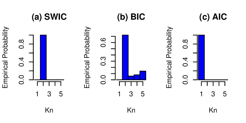
Model selection criteria. For each GMoE with $k$ experts, $k \in [5]$ , denote its parameter space by $𝒳_{k}$ . Following the suggestion of Sin & White (1996), when $τ_{n} = \sqrt{n}$ , we propose penalties of the form $P^{SWIC}_{k, n} = [dim (𝒳_{k}) \log (n)] / \sqrt{n}$ , defining what we designate the Sin and White information criterion (SWIC), where $dim (\cdot)$ is the number of parameters for each model. It is easy to verify that $P^{SWIC}_{k, n}$ satisfies F2. The usual BIC and AIC, with penalties $P^{BIC}_{k, n} = [dim (𝒳_{k}) \log (n)] / (2 n)$ and $P^{AIC}_{k, n} = dim (𝒳_{k}) / n$ , do not satisfy F2. To compute the MERs, we implement the usual Expectation–Maximization algorithm for GMoE models (see, e.g., Chamroukhi et al., 2009). Figure 1 displays the relative performance of the SWIC versus the BIC and AIC, over 50 simulations of size $n = 2000$ . We observe that SWIC correctly estimates $k^{*}$ in all replications, whereas AIC always underestimates the complexity. BIC estimates correctly with high probability (0.72) but often overestimates the complexity.

Refer to caption — Figure 1: Histogram of computed $\hat{K}_{n}$ over 50 simulations.

7.2 Neural Network

Here we seek to numerically verify the ability of the bootstrap procedures to generate asymptotically correct quantiles. We do this by using a model for which $ψ^{*}$ is analytically computable and test if the bootstrap procedures can generate confidence interval (CI) with the correct coverage.

To generate the model we consider a binary classification feedforward neural network (NN) with 1 input node and 1 hidden layer, consisting of 3 nodes with ReLU activation. We first fix a NN and generate $n$ IID replicates $(Z_{i})_{i \in ℕ}$ of $Z = (X, Y)$ , where $X \sim Unif (0, 1)$ and $Y$ is the output of the NN, with input $X$ , flipped 30% of the time.

We fit a NN with the same configuration to the data. Via the data generating process, we know that the minimum classification loss is $ψ^{*} = 0.3$ , by Lemma D.42. These networks were fit by minimising the classification loss using the ‘particleswarm’ global optimizer in MATLAB. Full details are given in Appendix D.

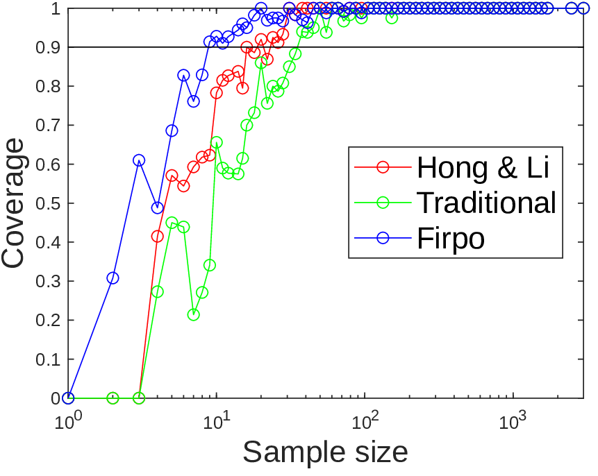
We seek to compute 90% CIs for the classification loss, using the standard nonparametric bootstrap and the two consistent procedures of Theorem 5.10. Figure 2 shows the coverage of these procedures. Note that for moderately large samples, all methods provide conservative coverage.

Our choice of NN configuration characterizes a class, $ℱ$ , of binary output functions, which is Donsker if $ℱ$ is a measurable VC subgraph class (cf. Dudley, 1999, Cor. 10.1.5). Since the classification loss of the NN can be evaluated with only a finite number of logical comparison and elementary arithmetic operations, the fact that $ℱ$ is a VC subgraph class then follows via Anthony & Bartlett (1999, Thm. 8.14). Theorem 5.10 implies that our methods should correctly provide $90 %$ coverage if the limiting distribution of the MER is continuous, while there is minimal support for the standard nonparametric bootstrap in this setting.

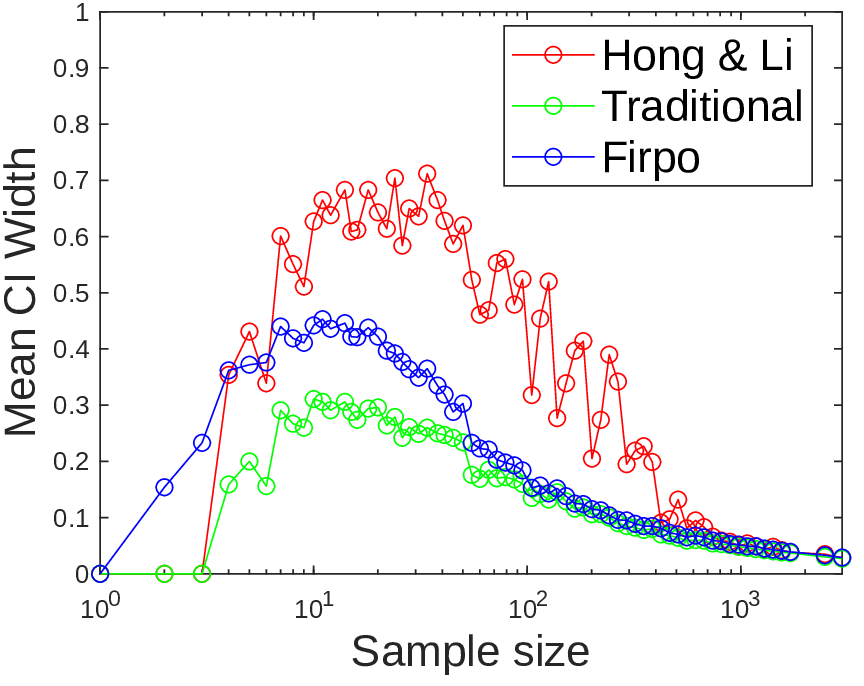
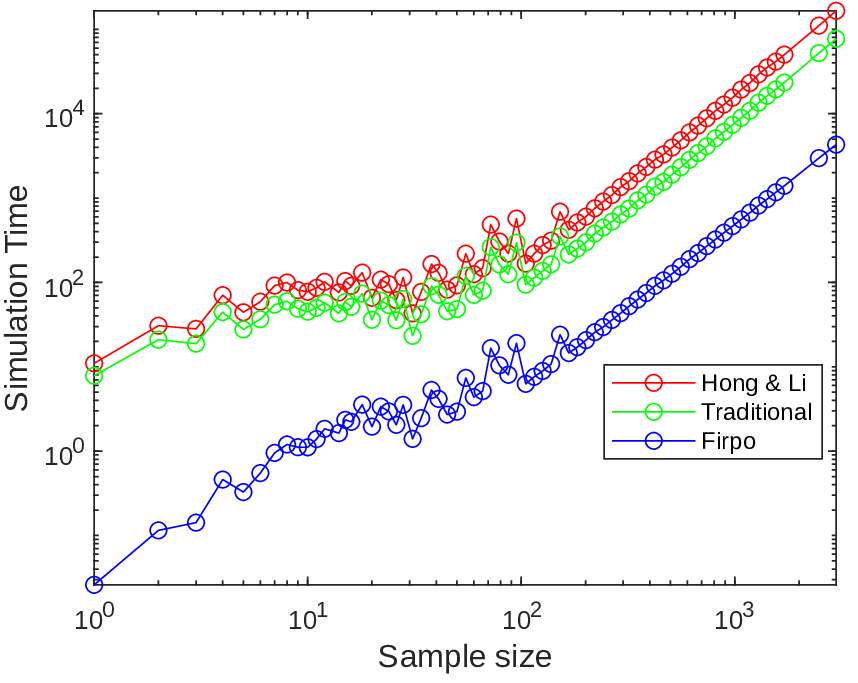
Figure 3 shows that the widths of the CIs are of reasonable sizes for moderate amount of data. For this numerical experiment, all bootstrap procedures achieved the nominal coverage. All methods do not take the same amount of computation resources, however (see Figure 4). The method based on Firpo et al. (2023) was considerably faster than the others due to the amortisation property of not requiring refits of the NN for each bootstrap resample.

8 Conclusion

We have reported on a comprehensive set of tools for characterizing the asymptotic distribution of MERs along with protocols for model selection and statistical inference, based on these theoretical results. Practical regularity conditions for implementing our methods and example applications are provided to illustrate the utility of our results. Further directions of study will involve better understanding the properties of the limiting distributions of MERs and how these properties interact with various bootstrap methods.

Acknowledgements

We thank the Reviewers and Area Chair whose advice helped to improve our manuscript. All authors acknowledge funding from the ARC grant: DP230100905.

Impact Statement

This paper presents work whose goal is to advance the field of Machine Learning. There are many potential societal consequences of our work, none which we feel must be specifically highlighted here.

References

Akaike (1974) Akaike, H. A new look at the statistical model identification. IEEE Transactions on Automatic Control, 19:716–723, 1974. ↩ 5
Amemiya (1985) Amemiya, T. Advanced econometrics. Harvard University Press, 1985. ↩ 1
Anthony & Bartlett (1999) Anthony, M. and Bartlett, P. L. Neural Network Learning: Theoretical Foundations. Cambridge University Press, Cambridge, 1999. ↩ 7.2
Azaïs et al. (2009) Azaïs, J.-M., Gassiat, É., and Mercadier, C. The likelihood ratio test for general mixture models with or without structural parameter. ESAIM: Probability and Statistics, 13:301–327, 2009. ↩ 1
Banholzer et al. (2022) Banholzer, D., Fliege, J., and Werner, R. On rates of convergence for sample average approximations in the almost sure sense and in mean. Mathematical Programming, pp. 1–39, 2022. ↩ 1
Bartlett et al. (2006) Bartlett, P. L., Jordan, M. I., and McAuliffe, J. D. Convexity, classification, and risk bounds. Journal of the American Statistical Association, 101(473):138–156, 2006. ↩ D.1
Baudry (2015) Baudry, J.-P. Estimation and model selection for model-based clustering with the conditional classification likelihood. Electronic Journal of Statistics, 9:1041–1077, 2015. ↩ 5
Bickel & Doksum (2015) Bickel, P. J. and Doksum, K. A. Mathematical statistics: basic ideas and selected topics, volume 1. CRC Press, 2015. ↩ 1
Bonnans (2019) Bonnans, J. F. Convex and stochastic optimization. Springer, 2019. ↩ 1
Bradley (2005) Bradley, R. C. Basic properties of strong mixing conditions. a survey and some open questions. Probability Surveys, 2:107–144, 2005. ↩ 3
Bücher & Kojadinovic (2019) Bücher, A. and Kojadinovic, I. A note on conditional versus joint unconditional weak convergence in bootstrap consistency results. Journal of Theoretical Probability, 32(3):1145–1165, 2019. ↩ 5
Bühlmann (1995) Bühlmann, P. The blockwise bootstrap for general empirical processes of stationary sequences. Stochastic Processes and their Applications, 58:247–265, 1995. ↩ 5
Carcamo et al. (2020) Carcamo, J., Cuevas, A., and Rodriguez, L.-A. Directional differentiability for supremum-type functionals: Statistical applications. Bernoulli, 26:2143–2175, 2020. ↩ 1 3 B B.2
Chamroukhi et al. (2009) Chamroukhi, F., Samé, A., Govaert, G., and Aknin, P. Time series modeling by a regression approach based on a latent process. Neural Networks, 22:593–602, 2009. Publisher: Elsevier. ↩ 7.1
Claeskens & Hjort (2008) Claeskens, G. and Hjort, N. L. Model selection and model averaging. Cambridge University Press, 2008. ↩ 5
Cucker & Zhou (2007) Cucker, F. and Zhou, D. X. Learning theory: an approximation theory viewpoint. Cambridge University Press, 2007. ↩ 1
Dacunha-Castelle & Duflo (1986) Dacunha-Castelle, D. and Duflo, M. Probability and Statistics: Volume II. Springer, 1986. ↩ 1
Dalalyan & Collier (2012) Dalalyan, A. and Collier, O. Wilks’ phenomenon and penalized likelihood-ratio test for nonparametric curve registration. In Artificial Intelligence and Statistics, pp. 264–272. PMLR, 2012. ↩ 1
Dedecker & Louhichi (2002) Dedecker, J. and Louhichi, S. Maximal inequalities and empirical central limit theorems. In Empirical Process Techniques for Dependent Data, pp. 137–159. Springer, 2002. ↩ 4
Dellacherie & Meyer (1975) Dellacherie, C. and Meyer, P.-A. Probabilities and Potential. Elsevier, 1975. ↩ 5
Doukhan (1995) Doukhan, P. Mixing: properties and examples. Springer, 1995. ↩ 4
Dudley (1999) Dudley, R. M. Uniform Central Limit Theorems. Cambridge University Press, 1999. ↩ 1 3 4 7.2
Fan et al. (2001) Fan, J., Zhang, C., and Zhang, J. Generalized likelihood ratio statistics and wilks phenomenon. The Annals of statistics, 29:153–193, 2001. ↩ 1
Fang & Santos (2019) Fang, Z. and Santos, A. Inference on directionally differentiable functions. The Review of Economic Studies, 86:377–412, 2019. ↩ 1 5 A.4
Firpo et al. (2023) Firpo, S., Galvao, A. F., and Parker, T. Uniform inference for value functions. Journal of Econometrics, 235:1680–1699, 2023. ↩ 1 5 7.2
Gao & Yiu (2023) Gao, M. and Yiu, K.-F. C. Moderate deviations and invariance principles for sample average approximations. SIAM Journal on Optimization, 33:816–841, 2023. ↩ 1
Gourieroux & Monfort (1995) Gourieroux, C. and Monfort, A. Statistics and Econometric Models, volume 2. Cambridge University Press, 1995. ↩ 1
Ho et al. (2022) Ho, N., Yang, C.-Y., and Jordan, M. I. Convergence rates for Gaussian mixtures of experts. Journal of Machine Learning Research, 23:1–81, 2022. ↩ 7.1
Hong & Li (2018) Hong, H. and Li, J. The numerical delta method. Journal of Econometrics, 206:379–394, 2018. ↩ 5 A.4
Hong & Li (2020) Hong, H. and Li, J. The numerical bootstrap. The Annals of Statistics, 48:397–412, 2020. ↩ 1
Jacobs et al. (1991) Jacobs, R. A., Jordan, M. I., Nowlan, S. J., and Hinton, G. E. Adaptive mixtures of local experts. Neural computation, 3(1):79–87, 1991. Publisher: MIT Press. ↩ 7.1
Kim et al. (2015) Kim, S., Pasupathy, R., and Henderson, S. G. A guide to sample average approximation. Handbook of simulation optimization, pp. 207–243, 2015. ↩ 1
Koltchinskii (2011) Koltchinskii, V. Oracle Inequalities in Empirical Risk Minimization and Sparse Recovery Problems: École D’Été de Probabilités de Saint-Flour XXXVIII-2008. Springer, 2011. ↩ 1
Kosorok (2008) Kosorok, M. R. Introduction to empirical processes and semiparametric inference, volume 61. Springer, 2008. ↩ 4 5
Liu & Singh (1992) Liu, R. Y. and Singh, K. Moving blocks jackknife and bootstrap capture weak dependence. In Exploring the Limits of Bootstrap, pp. 225–248. Wiley, 1992. ↩ 5
Nguyen et al. (2023) Nguyen, H., Nguyen, T., and Ho, N. Demystifying Softmax Gating Function in Gaussian Mixture of Experts. In Thirty-seventh Conference on Neural Information Processing Systems, 2023. ↩ 7.1
Nguyen et al. (2022) Nguyen, T., Nguyen, H. D., Chamroukhi, F., and Forbes, F. A non-asymptotic approach for model selection via penalization in high-dimensional mixture of experts models. Electronic Journal of Statistics, 16:4742 – 4822, 2022. ↩ 7.1
Papanastassiou (2020) Papanastassiou, N. A note on convergence of sequences of functions. Topology and its Applications, 275:107017, 2020. ↩ A.9
Radulović (2002) Radulović, D. On the bootstrap and empirical processes for dependent sequences. In Empirical Process Techniques for Dependent Data, pp. 345–364. Springer, 2002. ↩ 5
Römisch (2014) Römisch, W. Delta method, infinite dimensional. Wiley StatsRef: Statistics Reference Online, 2014. ↩ 1 3 A.1
Royset & Szechtman (2013) Royset, J. O. and Szechtman, R. Optimal budget allocation for sample average approximation. Operations Research, 61:762–776, 2013. ↩ 1
Schirotzek (2007) Schirotzek, W. Nonsmooth analysis. Springer Science & Business Media, 2007. ↩ 3
Schwarz (1978) Schwarz, G. Estimating the dimension of a model. The Annals of Statistics, 6:461–464, 1978. ↩ 5
Serfling (1980) Serfling, R. Approximation Theorems of Mathematical Statistics. John Wiley & Sons, Inc., Hoboken, 1980. ↩ 1
Shalev-Shwartz & Ben-David (2014) Shalev-Shwartz, S. and Ben-David, S. Understanding machine learning: From theory to algorithms. Cambridge university press, 2014. ↩ 1
Shapiro (1989) Shapiro, A. Asymptotic properties of statistical estimators in stochastic programming. The Annals of Statistics, 17:841–858, 1989. ↩ 1
Shapiro (1991) Shapiro, A. Asymptotic analysis of stochastic programs. Annals of Operations Research, 30:169–186, 1991. ↩ 1
Shapiro (2000) Shapiro, A. Statistical inference of stochastic optimization problems. In Probabilistic Constrained Optimization: Methodology and Applications, pp. 282–307. Springer, 2000. ↩ 1
Shapiro et al. (2021) Shapiro, A., Dentcheva, D., and Ruszczynski, A. Lectures on Stochastic Programming: Modeling and Theory. SIAM, 2021. ↩ 1 4 C
Sin & White (1996) Sin, C.-Y. and White, H. Information criteria for selecting possibly misspecified parametric models. Journal of Econometrics, 71:207–225, 1996. ↩ 5 7.1
Singh (1981) Singh, K. On the asymptotic accuracy of Efron’s bootstrap. Annals of Statistics, pp. 1187–1195, 1981. ↩ 5
van der Vaart & Wellner (2023) van der Vaart, A. and Wellner, J. Weak Convergence and Empirical Processes: With Applications to Statistics. Springer Science & Business Media, 2023. ↩ 1 2 3 4 5 A.5 A.7 A.9
Vapnik (1998) Vapnik, V. N. Statistical Learning Theory. Wiley, New York, 1998. ↩ 1
Vidyasagar (2003) Vidyasagar, M. Learning and generalisation: with applications to neural networks. Springer, London, 2003. ↩ 1
Vuong (1989) Vuong, Q. H. Likelihood ratio tests for model selection and non-nested hypotheses. Econometrica, pp. 307–333, 1989. ↩ 1
Wilks (1938) Wilks, S. S. The large-sample distribution of the likelihood ratio for testing composite hypotheses. The Annals of Mathematical Statistics, 9:60–62, 1938. ↩ 1
Willard (2012) Willard, S. General Topology. Courier Corporation, 2012. ↩ 6

Appendix A Proofs

A.1 Theorem 3.1

We have that for any $g \in ℓ^{\infty} (𝒜)$ , $g |_{ℬ} \in ℓ^{\infty} (ℬ)$ , and if $h_{n}$ converges to $h$ in $ℓ^{\infty} (𝒜)$ , then $h_{n} |_{ℬ}$ converges to $h |_{ℬ}$ in $ℓ^{\infty} (ℬ)$ . The result is then immediate by Römisch (2014, Prop. 1) with universe $ℬ$ .

A.2 Theorem 4.4

Let $ι$ be as in Theorem 3.1 with $𝒜 = 𝒳$ . This theorem gives that $ι$ is Hadamard directionally differentiable on $ℓ^{\infty} (𝒳)$ . By assumption $F (Ω) \subset ℓ^{\infty} (𝒳)$ , and we can modify $τ_{n} (\hat{f}_{n} - f)$ on $Ω ∖ Ω_{0}$ (where $ℙ (Ω_{0}) = 1$ ) so that it is also takes values in $ℓ^{\infty} (𝒳)$ . The conditions on the delta method (3.2) are then satisfied from which we get

τ_{n} (ι (\hat{f}_{n}) - ι (f)) ↝ ι^{'}_{f} (F), and

(12)

τ_{n} (ι (\hat{f}_{n}) - ι (f)) - ι_{f}^{'} (τ_{n} (\hat{f}_{n} - f)) = o_{ℙ^{*}} (1) .

(13)

By definition, $ι (\hat{f}_{n}) = \hat{ψ}_{n}$ and $ι (f) = ψ^{*}$ . Substituting in the expression for $ι^{'}_{f} (F)$ , given in Theorem 3.1, into Equation (12) gives Equation (3). Rearranging Equation (13) gives

	$τ_{n} (\hat{ψ}_{n} - ψ^{*})$	$= lim_{ϵ ↘ 0} inf_{x \in 𝒮^{ϵ}} (τ_{n} (\hat{f}_{n} (x) - f (x))) + o_{ℙ *} (1)$
	$⟹ \hat{ψ}_{n}$	$= lim_{ϵ ↘ 0} inf_{x \in 𝒮^{ϵ}} (\hat{f}_{n} (x) - f (x)) + ψ^{} + o_{ℙ } (τ_{n}^{- 1})$
		$= lim_{ϵ ↘ 0} inf_{x \in 𝒮^{ϵ}} (\hat{f}_{n} (x) - f (x) + ψ^{}) + o_{ℙ } (τ_{n}^{- 1}) .$

This is precisely Equation (4).

A.3 Corollary 4.6

Theorem 4.4 implies that

τ_{n} (\hat{ψ}_{n} - ψ^{*}) ↝ lim_{ϵ ↘ 0} inf_{x \in 𝒮^{ϵ}} F (x) .

If $𝒮^{ϵ}$ is constant and equal to $𝒮$ , for $ϵ$ sufficiently small, then

lim_{ϵ ↘ 0} inf_{x \in 𝒮^{ϵ}} F (x) = inf_{x \in 𝒮} F (x) .

Because $l$ is constant on $𝒮$ , $\hat{f}_{n}$ and $f$ is as well. Because $τ_{n} (\hat{f}_{n} - f) ↝ F$ , Lemma A.19 gives that $F$ is constant on $𝒳$ . Hence, for any $x^{*} \in 𝒮$

inf_{x \in 𝒮} F (x) = F (x^{*}) .

Lemma A.19.

Let $𝒳$ be a set and let $𝒜 \subseteq 𝒳$ . Let

𝒞_{𝒜} = {f \in ℓ^{\infty} (𝒳) : | f (𝒜) | = 1}

where $| \cdot |$ denotes set cardinality. Let $(Ω, 𝔉, ℙ)$ be a probability space, $X_{n} : Ω \to 𝒞_{𝒜}$ be maps, and $X : Ω \to ℓ^{\infty} (𝒳)$ be Borel measurable. If $X_{n} ↝ X$ then, $X : Ω \to 𝒞_{𝒜}$ .

Proof.

We first claim that $𝒞_{𝒜}$ is closed. To show this take $(f_{n}) \subset 𝒞_{𝒜}$ with $f_{n} \to f$ in $ℓ^{\infty} (𝒳)$ . We aim to show that $f \in 𝒞_{𝒜}$ . For the sake of contradiction assume $f \notin 𝒞_{𝒜}$ . This means $\exists a, b \in 𝒜$ such that $f (a) \neq f (b)$ . Without loss of generality assume $f (a) > f (b)$ (else relabel). Let $ϵ = (f (a) - f (b)) / 2$ . Then for $n$ sufficiently large,

| f_{n} (a) - f (a) | < ϵ and | f_{n} (b) - f (b) | < ϵ

which implies

- ϵ < f_{n} (a) - f (a) and f_{n} (b) - f (b) < ϵ .

By definition of $ϵ$ ,

\frac{f (b) - f (a)}{2} < f_{n} (a) - f (a) and f_{n} (b) - f (b) < \frac{f (a) - f (b)}{2}

and so

\frac{f (b) + f (a)}{2} < f_{n} (a) and f_{n} (b) < \frac{f (a) + f (b)}{2} .

That is, for $n$ large enough $f_{n} (a) > f_{n} (b)$ . However, $f_{n}$ is constant on $𝒜$ by assumption so we have a contradiction. It must then be true that $f \in 𝒞_{𝒜}$ and so $𝒞_{𝒜}$ is closed.

By the Portmanteau theorem, $\forall ℱ \subseteq ℓ^{\infty} (𝒳)$ closed,

lim sup_{n \to \infty} ℙ^{*} (X_{n} \in ℱ) \leq ℙ (X \in ℱ) .

Taking $ℱ = 𝒞_{𝒜}$ gives

1 = lim sup_{n \to \infty} ℙ^{*} (X_{n} \in 𝒞_{𝒜}) \leq ℙ (X \in 𝒞_{𝒜})

and so $ℙ (X \in 𝒞_{𝒜}) = 1$ . This is the required result (up to a possible modification on a null set). ∎

A.4 Theorem 5.10

Let $i_{n}$ generically denote one of $\hat{ι}_{s_{n}, n}^{'}$ or $\tilde{ι}^{'}_{t_{n}, n}$ . Our proof strategy is to verify the following assumptions:

(a)

$\sqrt{n} (\hat{f}_{n} - f) ↝ 𝔾$ , for some tight, Gaunssian $𝔾$ .
(b)

$\sqrt{n} (f^{b}_{n} - \hat{f}_{n}) | (Z_{i})_{i \in [n]} \overset{ℙ *}{↝} 𝔾$ .
(c)

$\sqrt{n} (f^{b}_{n} - \hat{f}_{n})$ is asymptotically measurable.
(d)

$\sqrt{n} (f^{b}_{n} - \hat{f}_{n})$ is a measurable function of the weights $(W_{i})_{i \in [n]}$ for fixed $(Z_{i})_{i \in [n]}$ .
(e)

The weights are chosen independent of the data
(f)

$\forall h_{1}, h_{2} \in ℓ^{\infty} (𝒳)$

$| i_{n} (h_{1}) - i_{n} (h_{2}) | \leq C_{n} ∥ h_{1} - h_{2} ∥_{𝒳},$

where $C_{n} = O_{ℙ^{*}} (1)$ .
(g)

$\forall h \in ℓ^{\infty} (𝒳)$

$i_{n} (h) \overset{ℙ *}{\to} lim_{ϵ ↘ 0} inf_{𝒮^{ϵ}} h .$

With all these assumptions along with the Hadamard directionally differentiability of $ι$ given in Theorem 3.1, the result follows from Fang & Santos (2019, Thm. 3.2).

Properties (a)–(e) are precisely D1-D4.

Properties (f) and (g) need to be verified for each estimator $\hat{ι}^{'}_{s_{n}, n}$ and $\tilde{ι}^{'}_{t_{n}, n}$ , separately.

For $\hat{ι}_{s_{n}, n}$ , (g) is given by Theorem 3.3 of Hong & Li (2018) and (f) follows by theorem 3.2 of Hong & Li (2018) if the $inf$ map is Lipschitz continuous. This is indeed true as for $h_{1}, h_{2} \in ℓ^{\infty} (𝒳)$ ,

| inf_{𝒳} h_{1} - inf_{𝒳} h_{2} | \leq sup_{𝒳} | h_{1} - h_{2} | = | | h_{1} - h_{2} | |_{𝒳} .

For $\tilde{ι}_{t_{n}, n}$ , (f) follows by a similar argument to the one above, as for any $𝒜 \subseteq 𝒳$ and $h_{1}, h_{2} \in ℓ^{\infty} (𝒳)$ ,

| inf_{𝒜} h_{1} - inf_{𝒜} h_{2} | \leq sup_{𝒜} | h_{1} - h_{2} | \leq | | h_{1} - h_{2} | |_{𝒳} .

In particular, the inequality above holds for $𝒜 = 𝒮^{t_{n}}_{n}$ . Because $τ_{n} (\hat{f}_{n} - f) ↝ F$ , Lemma A.22 implies that $τ_{n} (\hat{f}_{n} - f)$ is asymptotically bounded in probability in the sense that $\forall δ > 0$ , $\exists ℬ \subseteq 𝒳$ bounded s.t.

lim inf_{n \to \infty} ℙ_{*} (X_{n} \in ℬ) \geq 1 - δ

(g) then follows by Theorem A.20.

Theorem A.20.

Let $(Ω, 𝔉, ℙ)$ be a probability space, $𝒳$ a non-empty set, and $\hat{f}_{n}, f : Ω \to ℓ^{\infty} (𝒳)$ . If there is $τ_{n} \to \infty$ such that $τ_{n} (\hat{f}_{n} - f)$ is asymptotically bounded in probability, then for any $ϵ_{n} ↘ 0$ such that $ϵ_{n} τ_{n} \to \infty$ and any $h \in ℓ^{\infty} (𝒳)$ ,

inf_{𝒮_{n}^{ϵ_{n}}} h \overset{ℙ *}{\to} lim_{ϵ ↘ 0} inf_{𝒮^{ϵ}} h .

Proof.

We shall write $𝒮 (f, ϵ)$ to mean $𝒮^{ϵ}$ and $𝒮 (\hat{f}_{n}, ϵ)$ to mean $𝒮_{n}^{ϵ}$ . Fix $δ > 0$ . We are required to show

lim_{n \to \infty} ℙ^{*} (| inf_{𝒮 (\hat{f}_{n}, ϵ_{n})} h - lim_{ϵ ↘ 0} inf_{𝒮 (f, ϵ)} h | > δ) = 0 .

We firstly have

	$ℙ^{*} (\| inf_{𝒮 (\hat{f}_{n}, ϵ_{n})} h - lim_{ϵ ↘ 0} inf_{𝒮 (f, ϵ)} h \| > δ)$	$= ℙ^{*} ({inf_{𝒮 (\hat{f}_{n}, ϵ_{n})} h - lim_{ϵ ↘ 0} inf_{𝒮 (f, ϵ)} h > δ} \cup {inf_{𝒮 (\hat{f}_{n}, ϵ_{n})} h - lim_{ϵ ↘ 0} inf_{𝒮 (f, ϵ)} h < - δ})$
		$\leq ℙ^{} (inf_{𝒮 (\hat{f}_{n}, ϵ_{n})} h - lim_{ϵ ↘ 0} inf_{𝒮 (f, ϵ)} h > δ) + ℙ^{} (inf_{𝒮 (\hat{f}_{n}, ϵ_{n})} h - lim_{ϵ ↘ 0} inf_{𝒮 (f, ϵ)} h < - δ) .$

It then suffices to show that each of these outer probabilities tend to 0. We have

	$𝒮 (\hat{f}_{n}, ϵ_{n})$	$= {x \in 𝒳 : \hat{f}_{n} (x) \leq inf_{𝒳} \hat{f}_{n} + ϵ_{n}}$
		$= {x \in 𝒳 : \hat{f}_{n} (x) + f (x) - f (x) \leq inf_{𝒳} (\hat{f}_{n} - f + f) + ϵ_{n}}$
		$\subseteq {x \in 𝒳 : f (x) - ∥ \hat{f}_{n} - f ∥_{𝒳} \leq inf_{𝒳} f + ∥ \hat{f}_{n} - f ∥_{𝒳} + ϵ_{n}}$
		$= 𝒮 (f, ϵ_{n} + 2 ∥ \hat{f}_{n} - f ∥_{𝒳})$

We hence get

inf_{𝒮 (\hat{f}_{n}, ϵ_{n})} h \geq inf_{𝒮 (f, ϵ_{n} + ∥ \hat{f}_{n} - f ∥_{𝒳})} h

and so

ℙ^{*} (inf_{𝒮 (\hat{f}_{n}, ϵ_{n})} h - lim_{ϵ ↘ 0} inf_{𝒮 (f, ϵ)} h < - δ) \leq ℙ^{*} (inf_{𝒮 (f, ϵ_{n} + ∥ \hat{f}_{n} - f ∥_{𝒳})} h - lim_{ϵ ↘ 0} inf_{𝒮 (f, ϵ)} h < - δ) .

Then, observe that when $η ↘ 0$ , we have

inf_{𝒮 (f, η)} h ↗ lim_{ϵ ↘ 0} inf_{𝒮 (f, ϵ)} h,

and hence, there is some $η_{δ} > 0$ such that $\forall η < η_{δ}$

inf_{𝒮 (f, η)} h - lim_{ϵ ↘ 0} inf_{𝒮 (f, ϵ)} h \geq - δ .

By Lemma A.21, $| | \hat{f}_{n} - f | |_{𝒳} = o_{ℙ^{*}} (1)$ and because $ϵ_{n} ↘ 0$ ,

ℙ_{*} (ϵ_{n} + 2 ∥ f_{n} - f ∥_{𝒳} < η_{δ}) \to 1

By definition of $η_{δ}$ this gives

ℙ^{*} (inf_{𝒮 (f + ϵ_{n} + 2 ∥ \hat{f}_{n} - f ∥_{𝒳})} h - lim_{ϵ ↘ 0} inf_{𝒮 (f, ϵ)} h < - δ) \to 0 .

and so

ℙ^{*} (inf_{𝒮 (\hat{f}_{n}, ϵ_{n})} h - lim_{ϵ ↘ 0} inf_{𝒮 (f, ϵ)} h < - δ) \to 0 .

Hence, we are done if we can show that

ℙ^{*} (inf_{𝒮 (\hat{f}_{n}, ϵ_{n})} h - lim_{ϵ ↘ 0} inf_{𝒮 (f, ϵ)} h > δ) \to 0 .

Via a similar argument to above we get

𝒮 (\hat{f}_{n}, ϵ_{n}) \supseteq 𝒮 (f, ϵ_{n} - 2 ∥ \hat{f}_{n} - f ∥_{𝒳})

and therefore

inf_{𝒮 (\hat{f}_{n}, ϵ_{n})} h \leq inf_{𝒮 (f, ϵ_{n} - 2 ∥ \hat{f}_{n} - f ∥_{𝒳})} h .

We then have

ℙ^{*} (inf_{𝒮 (\hat{f}_{n}, ϵ_{n})} h - lim_{ϵ ↘ 0} inf_{𝒮 (f, ϵ)} h > δ) \leq ℙ^{*} (inf_{𝒮 (f, ϵ_{n} - 2 | | \hat{f}_{n} - f | |_{𝒳})} h - lim_{ϵ ↘ 0} inf_{𝒮 (f, ϵ)} h > δ) .

Because for any $η > 0$ ,

inf_{𝒮 (f, η)} h \leq lim_{ϵ ↘ 0} inf_{𝒮 (f, ϵ)} h

the result follows if

ℙ_{*} (ϵ_{n} - 2 | | \hat{f}_{n} - f | |_{𝒳} > 0) \to 1 .

Because $τ_{n} (\hat{f}_{n} - f)$ is asymptotically bounded in probability, $\forall η > 0$ , $\exists M \in ℝ$ such that for $n$ large enough

ℙ_{*} (| | \hat{f}_{n} - f | |_{𝒳} < \frac{M}{τ_{n}}) > 1 - η

which is equivalent to

ℙ_{*} (ϵ_{n} - 2 ∥ \hat{f}_{n} - f ∥_{𝒳} > ϵ_{n} - \frac{2 M}{τ_{n}}) > 1 - η .

It then suffices to show that for $n$ large enough,

ϵ_{n} - \frac{2 M}{τ_{n}} > 0

as this would give for $n$ large enough

ℙ_{*} (ϵ_{n} - 2 ∥ \hat{f}_{n} - f ∥_{𝒳} > ϵ_{n} - \frac{2 M}{τ_{n}}) \leq ℙ_{*} (ϵ_{n} - 2 ∥ \hat{f}_{n} - f ∥_{𝒳} > 0)

and hence give

lim inf_{n \to \infty} ℙ_{*} (ϵ_{n} - 2 ∥ \hat{f}_{n} - f ∥_{𝒳} > 0) \geq 1 - η

The result then follows by sending $η$ to 0. Rearrangement of this expression yields

ϵ_{n} τ_{n} > 2 M,

which is true for $n$ large enough as $ϵ_{n} τ_{n} \to \infty$ . ∎

Lemma A.21.

Let $(Ω, 𝔉, ℙ)$ be a probability space, $𝒳$ a normed space, and $\forall n \in ℕ$ let $X_{n} : Ω \to 𝒳$ maps. If there is a sequence $(τ_{n})_{n \in ℕ}$ with $τ_{n} \to \infty$ such that $τ_{n} X_{n}$ is asymptotically bounded in probability, then $X_{n} \overset{ℙ *}{\to} 0$

Proof.

We aim to show that $\forall ϵ > 0$

lim_{n \to \infty} ℙ_{*} (| | X_{n} | | < ϵ) = 1

Fix an $ϵ > 0$ . Then because $τ_{n} X_{n}$ is asymptotically bounded in probability $\forall δ > 0$ , $\exists M > 0$ such that

lim inf_{n \to \infty} ℙ_{*} (| | τ_{n} X_{n} | | < M) = lim inf_{n \to \infty} ℙ_{*} (| | X_{n} | | < M / τ_{n}) \geq 1 - δ

For $n$ large enough

ℙ_{*} (| | X_{n} | | < M / τ_{n}) \leq ℙ_{*} (| | X_{n} | | < ϵ)

and so $\forall δ > 0$

lim inf_{n \to \infty} ℙ_{*} (| | X_{n} | | < ϵ) \geq 1 - δ

Sending $δ \to 0$ gives

lim inf_{n \to \infty} ℙ_{*} (| | X_{n} | | < ϵ) \geq 1

which is equivalent to

lim_{n \to \infty} ℙ_{*} (| | X_{n} | | < ϵ) = 1

This is exactly what we wanted to show. ∎

Lemma A.22.

Let $(Ω, 𝔉, ℙ)$ be a probability space, $𝒳$ a metric space, $X : Ω \to 𝒳$ Borel measurable and $\forall n \in ℕ$ let $X_{n} : Ω \to 𝒳$ be maps. If $X_{n} ↝ X$ then $(X_{n})_{n \in ℕ}$ is asymptotically bounded in probability.

Proof.

Fix $δ > 0$ . We have

ℙ (X \in ⋃_{m = 1}^{\infty} B (0, m)) = 1

and so by continuity from below $\exists m \in ℕ$ such that

ℙ (X \in B (0, m)) \geq 1 - δ

By the Portmanteau theorem we have

lim inf_{n \to \infty} ℙ_{*} (X_{n} \in B (0, m)) \geq ℙ (X \in B (0, m))

Combining these 2 inequalities gives the result. ∎

A.5 Corollary 5.11

D1 is satisfied by definition of Donsker. D2 follows by $ℋ$ being Donsker by Theorem 3.7.1 of van der Vaart & Wellner (2023). For D3, $\sqrt{n} (f^{b}_{n} - \hat{f}_{n})$ as a function of the weights is simply a linear combination of elements of $ℓ^{\infty} (𝒳)$ . Measurability follows by Lemma A.23. D4 is clear.

Lemma A.23.

Let $𝒳$ be a set. For any $n \in ℕ$ and fixed $f_{1}, \dots, f_{n} \in ℓ^{\infty} (𝒳)$ , let $s : ℝ^{n} \to ℓ^{\infty} (𝒳)$ be given by

s (a_{1}, \dots, a_{n}) = \sum_{i = 1}^{n} a_{i} f_{i} .

The $s$ is Borel measurable.

Proof.

Because $ℝ^{n}$ and $ℓ^{\infty} (𝒳)$ are equipped with their Borel $σ$ -algebras it suffices to show that $s$ is continuous. We will actually show that $s$ is Lipschitz continuous.

	$\| \| s (a) - s (b) \| \|_{𝒳}$	$= ∥ \sum_{i = 1}^{n} (a_{i} - b_{i}) f_{i} ∥_{𝒳}$
		$\leq \sum_{i = 1}^{\infty} \| \| (a_{i} - b_{i}) f_{i} \| \|_{𝒳}$
		$\leq \sum_{i = 1}^{\infty} \| a_{i} - b_{i} \| ∥ f_{i} ∥_{𝒳}$
		$\leq \max_{i \in [n]} ∥ f_{i} ∥_{𝒳} ∥ a - b ∥_{1}$
		$\leq n \max_{i \in [n]} ∥ f_{i} ∥_{𝒳} ∥ a - b ∥_{2}$

Hence, $s$ is Lipschitz continuous with Lipschitz constant at most $n \max_{i \in [n]} ∥ f_{i} ∥_{𝒳}$ . ∎

A.6 Theorem 5.12

Let $ι_{0}, ι_{1} : ℓ^{\infty} (𝒳) \to ℝ$ given by

ι_{i} (f) = inf_{x \in 𝒳_{i}} f (x)

By Theorem 3.1, $ι_{i}$ is Hadamard directionally differentiable with derivative

ι_{i, f}^{'} (g) = lim_{ϵ ↘ 0} inf_{x \in 𝒮 (f, ϵ, 𝒳_{i})} g (x) .

In particular we have for any $g_{n} \to g$ in $ℓ^{\infty} (𝒳)$ ,

τ_{n} (\begin{matrix} ι_{1} (f + g_{n} / τ_{n}) - ι_{1} (f) \\ ι_{0} (f + g_{n} / τ_{n}) - ι_{0} (f) \end{matrix}) \to (\begin{matrix} ι_{1, f}^{'} (g) \\ ι_{0, f}^{'} (g) . \end{matrix})

That is, $(ι_{1}, ι_{0})^{⊤}$ is Hadamard directionally differentiable. Modify $\hat{f}_{n}$ on $Ω ∖ Ω_{0}$ so that $\hat{f}_{n}$ is bounded. All the conditions on the delta method (3.2) are satisfied. We then get.

τ_{n} (\begin{matrix} \hat{ψ}_{1, n} - ψ^{*}_{1} \\ \hat{ψ}_{0, n} - ψ^{*}_{0} \end{matrix}) ↝ (\begin{matrix} lim_{ϵ ↘ 0} inf_{x \in 𝒮 (f, ϵ, 𝒳_{1})} F (x) \\ lim_{ϵ ↘ 0} inf_{x \in 𝒮 (f, ϵ, 𝒳_{0})} F (x) \end{matrix})

Apply continuous mapping with the map $e : ℝ \times ℝ \to ℝ$ , $e (x, y) = x - y$ gives

τ_{n} (\hat{ψ}_{1, n} - ψ^{*}_{1} - \hat{ψ}_{0, n} + ψ^{*}_{0}) ↝ lim_{ϵ ↘ 0} inf_{x \in 𝒮 (f, ϵ, 𝒳_{1})} F (x) - lim_{ϵ ↘ 0} inf_{x \in 𝒮 (f, ϵ, 𝒳_{0})} F (x) .

Because $ψ^{*}_{1} = ψ^{*}_{0}$ , this is the required result.

A.7 Corollary 5.13

Theorem 5.12 implies that

τ_{n} (\hat{ψ}_{1, n} - \hat{ψ}_{0, n}) ↝ F^{*} .

The Portmanteau theorem (see van der Vaart & Wellner, 2023, Thm. 1.3.4) gives this is equivalent to

lim sup_{n \to \infty} ℙ^{*} (τ_{n} (\hat{ψ}_{1, n} - \hat{ψ}_{0, n}) \in 𝒞) \leq ℙ (F^{*} \in 𝒞)

for all closed $𝒞 \subseteq ℝ$ . In particular, if we take $𝒞 = (- \infty, c]$ , for $c \in \bar{ℝ}$ , we get

lim sup_{n \to \infty} ℙ^{*} (τ_{n} (\hat{ψ}_{1, n} - \hat{ψ}_{0, n}) \leq c) \leq ℙ (F^{*} \leq c)

We then have for any $c$ for which $ℙ (F^{*} \leq c) \leq α$ ,

lim sup_{n \to \infty} ℙ^{*} (τ_{n} (\hat{ψ}_{1, n} - \hat{ψ}_{0, n}) \leq c) \leq α .

In particular, it holds for the largest $c$ with this property:

c_{α} = sup {c \in \bar{ℝ} : ℙ (F^{*} \leq c) \leq α} .

We have therefore shown that

lim sup_{n \to \infty} ℙ^{*} (τ_{n} (\hat{ψ}_{1, n} - \hat{ψ}_{0, n}) \leq c_{α}) \leq α .

The LHS rearranges to give the required result.

A.8 Proposition 5.14

Let

𝒦 = \underset{k \in [m]}{\arg \min} ψ^{*}_{k} .

Because $[m]$ is finite this, as well as $k^{*}$ and $\hat{K}_{n}$ , are well defined.

Note that by Lemma A.21, F1 implies that $\hat{ψ}_{k, n} \overset{ℙ *}{\to} ψ_{k}^{*}$ , for each $k \in [m]$ . Together with F2, we get $\forall ϵ > 0$ and $\forall k \in [m]$ , the sets

{ω : | \hat{ψ}_{k, n} - ψ^{*}_{k} | < \frac{ϵ}{2}}, and {ω : P_{k, n} < \frac{ϵ}{2}}

have inner probability tending to 1. On the intersection of these events

	$\hat{ψ}_{k, n} + P_{k, n}$	$> \hat{ψ}_{k, n} - P_{k, n}$
		$> \hat{ψ}_{k, n} - \frac{ϵ}{2}$
		$> ψ^{*}_{k} - ϵ$
For $k \notin 𝒦$ we can take $ϵ = (ψ_{k}^{} - ψ^{}_{k^{*}}) / 2$ (note $ϵ > 0$ ) to get
		$= ψ_{k}^{} - \frac{ψ_{k}^{} - ψ_{k^{}}^{}}{2}$
		$= \frac{ψ_{k}^{} + ψ_{k^{}}^{*}}{2}$
		$= ψ_{k^{}}^{} + \frac{ψ_{k}^{} - ψ_{k^{}}^{*}}{2}$
		$= ψ^{}_{k^{}} + ϵ$
		$> \hat{ψ}_{k^{*}, n} + \frac{ϵ}{2}$
		$> \hat{ψ}_{k^{}, n} + P_{k^{}, n}$

Because $[m]$ is finite, on

\tilde{Ω}_{n} : = ⋂_{k \notin 𝒦} {ω : | \hat{ψ}_{k, n} - ψ^{*}_{k} | < \frac{ϵ}{2}} \cap {ω : P_{k, n} < \frac{ϵ}{2}},

we have

inf_{k \notin 𝒦} (\hat{ψ}_{k, n} + P_{k, n}) > \hat{ψ}_{k^{*}, n} + P_{k^{*}, n} .

Because $\tilde{Ω}_{n}$ is the finite intersection of sets whose inner probability tends to 1, $ℙ_{*} (\tilde{Ω}_{n}) \to 1$ .

Fix $k \in 𝒦$ and $ϵ > 0$ . By definition of asymptotically bounded in probability, $\exists M_{1}, M_{2} \in ℝ$ such that for $n$ large enough,

	$ℙ_{} (τ_{n} \| \hat{ψ}_{k, n} - ψ^{}_{k} \| < M_{1})$	$\geq 1 - \frac{ϵ}{2},$
	$ℙ_{} (τ_{n} \| \hat{ψ}_{k^{}, n} - ψ^{}_{k^{}} \| < M_{2})$	$\geq 1 - \frac{ϵ}{2} .$

which are of course equivalent to

	$ℙ_{} (- M_{1} < τ_{n} (\hat{ψ}_{k, n} - ψ^{}_{k}) < M_{1})$	$\geq 1 - \frac{ϵ}{2},$
	$ℙ_{} (- M_{2} < τ_{n} (ψ^{}_{k^{}} - \hat{ψ}_{k^{}, n}) < M_{2})$	$\geq 1 - \frac{ϵ}{2} .$

We hence obtain

ℙ_{*} (- M_{1} - M_{2} < τ_{n} (\hat{ψ}_{k, n} - ψ^{*}_{k}) - τ_{n} (\hat{ψ}_{k^{*}, n} - ψ^{*}_{k^{*}}) < M_{2} + M_{1}) \geq 1 - ϵ .

By definition of $𝒦$ , $ψ^{*}_{k} = ψ^{*}_{k^{*}}$ and so the above expression simplifies to

ℙ_{*} (- M_{1} - M_{2} < τ_{n} (\hat{ψ}_{k, n} - \hat{ψ}_{k^{*}, n}) < M_{2} + M_{1}) \geq 1 - ϵ

⟺ ℙ_{*} (τ_{n} | (\hat{ψ}_{k, n} - \hat{ψ}_{k^{*}, n}) | < M_{2} + M_{1}) \geq 1 - ϵ .

If $k \neq k^{*}$ , then $k > k^{*}$ and by F2 $τ_{n} (P_{k, n} - P_{k^{*}, n}) \overset{ℙ *}{\to} \infty$ . By definition for $n$ large enough

ℙ_{*} (P_{k, n} - P_{k^{*}, n} > (M_{1} + M_{2}) / τ_{n}) \geq 1 - ϵ .

Combining the above results we get for $n$ large enough

	$ℙ_{} (\| \hat{ψ}_{k, n} - \hat{ψ}_{k^{}, n} \| < \frac{M_{1} + M_{2}}{τ_{n}})$	$\geq 1 - ϵ,$
	$ℙ_{} (P_{k, n} - P_{k^{}, n} > \frac{M_{1} + M_{2}}{τ_{n}})$	$\geq 1 - ϵ .$

Let

\bar{Ω}_{k, n} = {ω : | \hat{ψ}_{k, n} - \hat{ψ}_{k^{*}, n} | < \frac{M_{1} + M_{2}}{τ_{n}}} \cap {ω : P_{k, n} - P_{k^{*}, n} > \frac{M_{1} + M_{2}}{τ_{n}}} .

Then on $\bar{Ω}_{k, n}$ we have

\hat{ψ}_{k^{*}, n} - \hat{ψ}_{k, n} < \frac{M_{1} + M_{2}}{τ_{n}} < P_{k, n} - P_{k^{*}, n}

⟹ \hat{ψ}_{k^{*}, n} + P_{k^{*}, n} < \hat{ψ}_{k, n} + P_{k, n}

Let

\bar{Ω}_{n} = ⋂_{k \in 𝒦} \bar{Ω}_{k, n}

Then $ℙ_{*} (\bar{Ω}_{n}) \geq 1 - 2 | 𝒦 | ϵ$ and on this set

\hat{ψ}_{k^{*}, n} + P_{k^{*}, n} < inf_{k \in 𝒦 ∖ {k^{*}}} (\hat{ψ}_{k, n} + P_{k, n}) .

Hence, $ℙ_{*} (\tilde{Ω}_{n} \cap \bar{Ω}_{n}) \to 1$ and on $\tilde{Ω}_{n} \cap \bar{Ω}_{n}$

\hat{ψ}_{k^{*}, n} + P_{k^{*}, n} < inf_{k \in [m] ∖ {k^{*}}} (\hat{ψ}_{k, n} + P_{k, n}) .

That is on $\tilde{Ω}_{n} \cap \bar{Ω}_{n}$

{k^{*}} = a r g m i n_{k \in [m]} (\hat{ψ}_{k, n} + P_{k, n})

and so in particular

k^{*} = \min [a r g m i n_{k \in 𝒦} (\hat{ψ}_{k, n} + P_{k, n})] .

I.e.

ℙ_{*} (\hat{K}_{n} = k^{*}) \to 1

as required.

A.9 Theorem 6.15

First proving

τ_{n} (g_{n} (X_{n}) - h_{n} (μ)) ↝ D_{μ} (X)

(14)

Define $d_{n} : 𝒰 \to 𝒱$ via

d_{n} (x) = τ_{n} (g_{n} (μ + x / τ_{n}) - h_{n} (μ))

By assumption, for any $η_{n} \to η$ , $g_{n} (η_{n}) \to D_{μ} (η)$ . Generalized continuous mapping then gives

d_{n} (τ_{n} (X_{n} - μ)) ↝ D_{μ} (X)

The expanded form of the LHS is

τ_{n} (g_{n} (X_{n}) - h_{n} (μ))

This is exactly Equation 14.

Now showing

τ_{n} (g_{n} (X_{n}) - h_{n} (μ)) - D_{μ} (τ_{n} (X_{n} - μ)) = o_{ℙ *} (1)

(15)

Next define $\tilde{d}_{n} : 𝒰 \to 𝒱 \times 𝒱$ via

\tilde{d}_{n} (x) = (\begin{matrix} d_{n} (x) \\ D_{μ} (x) \end{matrix})

Because $D_{μ} (x)$ is converged to continuously, it must be continuous (Papanastassiou, 2020, Prop. 2.5). By assumption and the continuity of $D_{μ}$ , for any $x_{n} \to x$

\tilde{d}_{n} (x_{n}) \to (D_{μ} (x), D_{μ} (x)) .

Generalized continuous mapping then gives

\tilde{d}_{n} (τ_{n} (X_{n} - μ)) ↝ (\begin{matrix} D_{μ} (X) \\ D_{μ} (X) \end{matrix})

The expanded form of the LHS is

(\begin{matrix} τ_{n} (g_{n} (X_{n}) - h_{n} (μ)) \\ D_{μ} (τ_{n} (X_{n} - μ)) . \end{matrix})

Applying continuous mapping (see (van der Vaart & Wellner, 2023, thrm 1.3.6)) with the map $s : 𝒱 \times 𝒱 \to 𝒱$ , $s (y_{1}, y_{2}) = y_{1} - y_{2}$ gives

τ_{n} (g (X_{n}) - g (μ)) - D_{μ} (τ_{n} (X_{n} - μ)) ↝ 0

Because weak convergence to a constant implies convergence in outer probability to that constant (see van der Vaart & Wellner, 2023, Lem. 1.10.2) we get

τ_{n} (g (X_{n}) - g (μ)) - D_{μ} (τ_{n} (X_{n} - μ)) \overset{ℙ *}{\to} 0

This is exactly Equation 15.

A.10 Theorem 6.16

In this section, for a general function $h : 𝒳 \to ℝ$ we write

𝒮 (h, ϵ) = {x \in 𝒳 : h (x) \leq inf_{𝒳} h + ϵ} .

First some helpful lemmas.

Lemma A.24.

Let $𝒳$ be a set and $\forall n \in ℕ$ let $𝒳_{n} \subseteq 𝒳$ . $\forall n \in ℕ$ let $f, g, g_{n} : 𝒳 \to \bar{ℝ}$ be bounded below with $| | g_{n} - g | |_{𝒳} \to 0$ and let $(t_{n}) \subseteq ℝ^{+}$ with $t_{n} \to 0$ . Then

lim_{n \to \infty} \frac{inf_{𝒳_{n}} (f + t_{n} g_{n}) - inf_{𝒳} (f)}{t_{n}} = lim_{n \to \infty} \frac{inf_{𝒳_{n}} (f + t_{n} g) - inf_{𝒳} (f)}{t_{n}}

provided either limit exists.

Proof.

If

lim_{n \to \infty} \frac{inf_{𝒳_{n}} (f + t_{n} g_{n}) - inf_{𝒳} (f)}{t_{n}}

exists then

	$\frac{inf_{𝒳_{n}} (f + t_{n} g_{n}) - inf_{𝒳} (f)}{t_{n}} - \| \| g_{n} - g \| \|_{𝒳}$	$\leq \frac{inf_{𝒳_{n}} (f + t_{n} g) - inf_{𝒳} (f)}{t_{n}}$
		$\leq \frac{inf_{𝒳_{n}} (f + t_{n} g_{n}) - inf_{𝒳} (f)}{t_{n}} + \| \| g_{n} - g \| \|_{𝒳}$

and so so the result follows by squeeze theorem. If

lim_{n \to \infty} \frac{inf_{𝒳_{n}} (f + t_{n} g) - inf_{𝒳} (f)}{t_{n}}

exists then

	$\frac{inf_{𝒳_{n}} (f + t_{n} g) - inf_{𝒳} (f)}{t_{n}} - \| \| g_{n} - g \| \|_{𝒳}$	$\leq \frac{inf_{𝒳_{n}} (f + t_{n} g_{n}) - inf_{𝒳} (f)}{t_{n}}$
		$\leq \frac{inf_{𝒳_{n}} (f + t_{n} g) - inf_{𝒳} (f)}{t_{n}} + \| \| g_{n} - g \| \|_{𝒳}$

and so the result again follows by squeeze theorem. ∎

Lemma A.25.

Let $𝒳$ be a set, $\forall n \in ℕ$ let $𝒳_{n} \subseteq 𝒳$ with $𝒳_{n} \neq \emptyset$ , $(t_{n}) \subseteq ℝ^{+}$ with $t_{n} \to 0$ , let $f, g : 𝒳 \to \bar{ℝ}$ be bounded below and let

lim_{n \to \infty} \frac{inf_{𝒳_{n}} f - inf_{𝒳} f}{t_{n}} = 0

Then

lim_{n \to \infty} \frac{inf_{𝒳_{n}} (f + t_{n} g) - inf_{𝒳} f}{t_{n}} = lim_{n \to \infty} \frac{inf_{𝒳_{n}} (f + t_{n} g) - inf_{𝒳_{n}} f}{t_{n}}

provided either limit exists.

Proof.

If

lim_{n \to \infty} \frac{inf_{𝒳_{n}} (f + t_{n} g) - inf_{𝒳} f}{t_{n}}

exists then we have

	$lim_{n \to \infty} \frac{inf_{𝒳_{n}} (f + t_{n} g) - inf_{𝒳} f}{t_{n}}$	$= lim_{n \to \infty} \frac{inf_{𝒳_{n}} (f + t_{n} g) - inf_{𝒳} f}{t_{n}} - lim_{n \to \infty} \frac{inf_{𝒳_{n}} f - inf_{𝒳} f}{t_{n}}$
		$= lim_{n \to \infty} \frac{inf_{𝒳_{n}} (f + t_{n} g) - inf_{𝒳_{n}} f}{t_{n}} .$

Similarly if

lim_{n \to \infty} \frac{inf_{𝒳_{n}} (f + t_{n} g) - inf_{𝒳_{n}} f}{t_{n}}

exists we have

	$lim_{n \to \infty} \frac{inf_{𝒳_{n}} (f + t_{n} g) - inf_{𝒳_{n}} f}{t_{n}}$	$= lim_{n \to \infty} \frac{inf_{𝒳_{n}} (f + t_{n} g) - inf_{𝒳_{n}} f}{t_{n}} + lim_{n \to \infty} \frac{inf_{𝒳_{n}} f - inf_{𝒳} f}{t_{n}}$
		$= lim_{n \to \infty} \frac{inf_{𝒳_{n}} (f + t_{n} g) - inf_{𝒳} f}{t_{n}} .$

∎

Lemma A.26.

Let $𝒳$ be a non-empty, compact, metric space and $\forall n \in ℕ$ let $𝒳_{n} \subseteq X$ be such that $𝒳_{1} \subseteq 𝒳_{2} \subseteq \dots$ and $𝒳 = ⋃_{n = 1}^{\infty} 𝒳_{n}$ . Let $f \in l s c (𝒳)$ and let $(t_{n}) \subseteq ℝ^{+}$ with $t_{n} \to 0$ .

Then

lim_{n \to \infty} \frac{inf_{𝒳_{n}} f - inf_{𝒳} f}{t_{n}} = 0

Proof.

Because $f$ is lsc and $𝒳$ is compact, by EVT $f$ attains it’s minima. Let $x_{0}$ be such a minimizer. Then $\exists N \in ℕ$ s.t. $\forall n > N$ , $x_{0} \in 𝒳_{n}$ . Hence $\forall n > N$ $inf_{𝒳_{n}} f = inf_{𝒳} f$ . The result is then immediate. ∎

Lemma A.27.

Let $𝒳$ be a compact metric space, and $f, g : 𝒳 \to ℝ$ be lower semi-continuous. Then

lim_{ϵ ↘ 0} inf_{𝒮^{ϵ}} g = inf_{𝒮} g .

Proof.

Recall the fact that a lower semi-continuous function achieves its minimum on a compact set and hence $𝒮 \neq \emptyset$ . Observe that for any $ϵ > 0$ , $𝒮^{ϵ} \supseteq 𝒮$ and hence

lim_{ϵ ↘ 0} inf_{𝒮^{ϵ}} g \leq inf_{𝒮} g .

(16)

Because $f$ is lsc, for any $ϵ > 0$ , $𝒮^{ϵ}$ is closed. Because $𝒳$ is compact we then have $𝒮^{ϵ}$ is compact. For any integer $n \geq 1$ , since $𝒮^{1 / n}$ is compact and $g$ is lower semi-continuous, there exists a minimizer $x_{n}$ ,

g (x_{n}) = inf_{𝒮^{1 / n}} g \leq lim_{ϵ ↘ 0} inf_{𝒮^{ϵ}} g .

Since $𝒳$ is compact, $(x_{n})$ has a converging subsequence, which we assume is just $(x_{n})$ itself, without loss of generality. Write $x_{0} = lim x_{n}$ . Since, $x_{n} \in 𝒮^{1 / n}$

f (x_{n}) \leq inf_{𝒳} f + \frac{1}{n}

and so

f (x_{0}) \leq lim inf_{n \to \infty} f (x_{n}) \leq inf_{𝒳} f

This implies $x_{0} \in 𝒮$ . Note that $(g (x_{n}))_{n \in ℕ}$ is a non-decreasing sequence and

inf_{x \in 𝒮 (f, 0)} g (x) \leq g (x_{0}) \leq lim_{n \to \infty} g (x_{n}) \leq lim_{ϵ ↘ 0} inf_{x \in 𝒮 (f, ϵ)} g (x) .

This, together with (16), completes the proof. ∎

Theorem A.28.

Let $𝒳$ be a non-empty, compact, metric space and $\forall n \in ℕ$ let $𝒳_{n} \subseteq 𝒳$ be such that $𝒳_{1} \subseteq 𝒳_{2} \subseteq \dots$ and $𝒳 = ⋃_{n = 1}^{\infty} 𝒳_{n}$ . Let $f \in l s c (𝒳)$ and let $(t_{n}) \subseteq ℝ^{+}$ with $t_{n} \to 0$ .

For any $g \in l s c (𝒳)$

inf_{𝒮 (f, 0)} g = lim_{n \to \infty} \frac{inf_{𝒳_{n}} (f + t_{n} g) - inf_{𝒳_{n}} f}{t_{n}}

Proof.

We will show

	$inf_{𝒮 (f, 0)} g$	$\leq lim inf_{n \to \infty} \frac{inf_{𝒳_{n}} (f + t_{n} g) - inf_{𝒳_{n}} f}{t_{n}} and$		(17)
	$inf_{𝒮 (f, 0)} g$	$\geq lim sup_{n \to \infty} \frac{inf_{𝒳_{n}} (f + t_{n} g) - inf_{𝒳_{n}} f}{t_{n}} .$		(18)

The combination of both will show the result.

First showing Equation 17. Take any $j_{n} > 0$ s.t. $j_{n} / t_{n} \to 0$ and take $x \in 𝒮_{n} (f + t_{n} g, j_{n})$ where

𝒮_{n} (f, ϵ) = {x \in 𝒳_{n} : f (x) \leq inf_{𝒳_{n}} f + ϵ}

Then

	$\frac{inf_{𝒳_{n}} (f + t_{n} g) - inf_{𝒳_{n}} f}{t_{n}}$	$\geq \frac{f (x) + t_{n} g (x) - j_{n} - f (x)}{t_{n}}$
		$= \frac{t_{n} g (x) - j_{n}}{t_{n}}$
		$= g_{n} (x) - \frac{j_{n}}{t_{n}}$
		$\geq inf_{𝒮_{n} (f + t_{n} g, j_{n})} g - \frac{j_{n}}{t_{n}}$
	$⟹ lim inf_{n \to \infty} \frac{inf_{𝒳_{n}} (f + t_{n} g) - inf_{𝒳_{n}} f}{t_{n}}$	$\geq lim inf_{n \to \infty} inf_{𝒮_{n} (f + t_{n} g, j_{n})} g$

We have

	$𝒮_{n} (f + t_{n} g, j_{n})$	$= {x \in 𝒳_{n} : f (x) + t_{n} g (x) \leq inf_{𝒳_{n}} (f + t_{n} g) + j_{n}}$
		$\subseteq {x \in 𝒳_{n} : f (x) - t_{n} \| \| g \| \|_{𝒳} \leq inf_{𝒳_{n}} f + t_{n} \| \| g \| \|_{𝒳} + j_{n}}$
		$= {x \in 𝒳_{n} : f (x) \leq inf_{𝒳_{n}} f + 2 t_{n} \| \| g \| \|_{𝒳} + j_{n}}$
		$= {x \in 𝒳_{n} : f (x) \leq inf_{𝒳} f + 2 t_{n} \| \| g \| \|_{𝒳} + j_{n} + inf_{𝒳_{n}} f - inf_{𝒳} f}$
		$= 𝒮 (f, 2 t_{n} \| \| g \| \|_{𝒳} + j_{n} + inf_{𝒳_{n}} f - inf_{𝒳} f) \cap 𝒳_{n}$
		$\subseteq 𝒮 (f, 2 t_{n} \| \| g \| \|_{𝒳} + j_{n} + inf_{𝒳_{n}} f - inf_{𝒳} f)$

Hence,

	$lim inf_{n \to \infty} \frac{inf_{𝒳_{n}} (f + t_{n} g) - inf_{𝒳_{n}} f}{t_{n}}$	$\geq lim inf_{n \to \infty} inf_{𝒮 (f, 2 t_{n} \| \| g \| \|_{𝒳} + j_{n} + inf_{𝒳_{n}} f - inf_{𝒳} f)} g .$
Because $2 t_{n} \| \| g \| \|_{𝒳} + j_{n} + inf_{𝒳_{n}} f - inf_{𝒳} f ↘ 0$
	$lim inf_{n \to \infty} inf_{𝒮 (f, 2 t_{n} \| \| g \| \|_{𝒳} + j_{n} + inf_{𝒳_{n}} f - inf_{𝒳} f)} g$	$= lim_{ϵ ↘ 0} inf_{𝒮 (f, ϵ)} g$
and so
	$lim inf_{n \to \infty} \frac{inf_{𝒳_{n}} (f + t_{n} g) - inf_{𝒳_{n}} f}{t_{n}}$	$\geq lim_{ϵ ↘ 0} inf_{𝒮 (f, ϵ)} g .$
By Lemma A.27
	$lim_{ϵ ↘ 0} inf_{𝒮 (f, ϵ)} g$	$= inf_{𝒮 (f, 0)} g .$
Finally, we have
	$lim inf_{n \to \infty} \frac{inf_{𝒳_{n}} (f + t_{n} g) - inf_{𝒳_{n}} f}{t_{n}}$	$\geq inf_{𝒮 (f, 0)} g .$

This is precisely Equation 17.

Now proving Equation 18. Fix $s_{n} > 0$ , such that $s_{n} / t_{n} \to 0$ and take $x \in S_{n} (f, s_{n})$ . Then

	$\frac{inf_{𝒳_{n}} (f + t_{n} g) - inf_{𝒳_{n}} f}{t_{n}}$	$\leq \frac{f (x) + t_{n} g (x) - f (x) + s_{n}}{t_{n}}$
		$= \frac{t_{n} g (x) + s_{n}}{t_{n}}$
		$= g (x) + \frac{s_{n}}{t_{n}}$
This is true for any $x$ so
	$\frac{inf_{𝒳_{n}} (f + t_{n} g) - inf_{𝒳_{n}} f}{t_{n}}$	$\leq inf_{𝒮_{n} (f, s_{n})} g + \frac{s_{n}}{t_{n}}$
	$⟹ lim sup_{n \to \infty} \frac{inf_{𝒳_{n}} (f + t_{n} g) - inf_{𝒳_{n}} f}{t_{n}}$	$\leq lim sup_{n \to \infty} inf_{𝒮_{n} (f, s_{n})} g$

We are then done if we can show that

lim sup_{n \to \infty} inf_{𝒮_{n} (f, s_{n})} g \leq lim_{ϵ ↘ 0} inf_{𝒮 (f, 0)} g

Because $f$ is lsc, $𝒮 (f, 0)$ is closed. Because $𝒳$ is compact, $S (f, 0)$ is then also compact. Then by EVT we have $inf_{𝒮 (f, 0)} g$ is attained. Let the point of attainment be $x^{*}$ . We have $\exists N \in ℕ$ s.t. $\forall n > N$ $x^{*} \in 𝒳_{n}$ . Then $\forall n > N$

inf_{S (f, 0)} g = g (x^{*}) = inf_{𝒮 (f, 0) \cap 𝒳_{n}} g \geq inf_{𝒮 (f, s_{n}) \cap 𝒳_{n}} g

Hence

lim sup_{n \to \infty} inf_{𝒮_{n} (f, s_{n}) \cap 𝒳_{n}} \leq inf_{S (f, 0)} g

which is the required result. ∎

Combining all this together we get the following result. This is precisely what we want to show.

Theorem A.29.

Let $𝒳$ be a non-empty, compact, metric space and $\forall n \in ℕ$ let $𝒳_{n} \subseteq X$ be such that $𝒳_{1} \subseteq 𝒳_{2} \subseteq \dots$ and $𝒳 = ⋃_{n = 1}^{\infty} 𝒳_{n}$ . Let $f \in l s c (𝒳)$ and let $(t_{n}) \subseteq ℝ^{+}$ with $t_{n} \to 0$ .

For any $g_{n}, g \in l s c (𝒳)$ with $| | g_{n} - g | |_{𝒳} \to 0$

	$inf_{𝒮 (f, 0)} g$	$= lim_{n \to \infty} \frac{inf_{𝒳_{n}} (f + t_{n} g_{n}) - inf_{𝒳} f}{t_{n}}, and$		(19)
	$inf_{𝒮 (f, 0)} g$	$= lim_{n \to \infty} \frac{inf_{𝒳_{n}} (f + t_{n} g_{n}) - inf_{𝒳_{n}} f}{t_{n}} .$		(20)

Proof.

Lemma A.24 gives that it suffices to show Gateaux differentiability. Lemma A.26 gives that the conditions on Lemma A.25 are satisfied and hence the Gateaux differentiable forms of Equation 8 and Equation 9 are equivalent. Theorem A.28 gives the Gateaux differentiable form of Equation 9. ∎

A.11 Theorem 6.17

Again, in this section, for a general function $h : 𝒳 \to ℝ$ we write

𝒮 (h, ϵ) = {x \in 𝒳 : h (x) \leq inf_{𝒳} h + ϵ} .

First some helpful results

Theorem A.30.

Let $𝒳$ be a set, and $\forall n \in ℕ$ let $𝒳_{n} \subseteq 𝒳$ . Let $(t_{n}) \subseteq ℝ^{+}$ with $t_{n} \to 0$ , $(j_{n}) \subseteq ℝ^{+}$ with $j_{n} / t_{n} \to 0$ , and let $f \in ℓ^{\infty} (𝒳)$ . If

lim_{n \to \infty} \frac{inf_{𝒳_{n}^{c}} f - inf_{𝒳} f}{t_{n}} = \infty,

(21)

then $\forall (g_{n})_{n \in ℕ} \subset ℓ^{\infty} (𝒳)$ uniformly bounded, $\exists N \in ℕ$ s.t. $\forall n > N$

S (f + t_{n} g_{n}, j_{n}) \cap 𝒳_{n} \neq \emptyset .

Proof.

Take any $(g_{n})_{n \in ℕ} \subset ℓ^{\infty} (𝒳)$ uniformly bounded and let the uniform bound be $C$ . That is, $\forall n \in ℕ$ , $| | g_{n} | |_{\infty} \leq C$ .

Because $j_{n} / t_{n} \to 0$ , $\exists N_{1} \in ℕ$ such that $\forall n > N_{1}$ , $j_{n} \leq t_{n} C$ . Similarly, Equation 21 gives that $\exists N_{2} \in ℕ$ such that $\forall n > N_{2}$

inf_{𝒳_{n}^{c}} f > inf_{𝒳} f + 3 t_{n} C

Take any $x \in 𝒮 (f + t_{n} g, j_{n})$ . By definition

	$f (x) + t_{n} g (x)$	$\leq inf_{𝒳} (f + t_{n} g_{n}) + j_{n}$
		$\leq inf_{𝒳} f + t_{n} sup_{𝒳} g_{n} + j_{n}$
	$⟹ f (x)$	$\leq inf_{𝒳} f + t_{n} (sup_{𝒳} g_{n} - g_{n} (x)) + j_{n}$
		$\leq inf_{𝒳} f + 2 t_{n} C + j_{n}$
If $n > N_{1}$ then
		$\leq inf_{𝒳} f + 3 t_{n} C$
If additionally $n > N_{2}$ then
		$< inf_{𝒳_{n}^{c}} f$

That is $\forall n > \max {N_{1}, N_{2}}$ , $f (x) < inf_{𝒳_{n}^{c}} f$ and so $x \in 𝒳_{n}$ . Hence, $\forall n > \max {N_{1}, N_{2}}$ $x \in 𝒮 (f + t_{n} g_{n}, j_{n}) \cap 𝒳_{n}$ and so in particular $\forall n > \max {N_{1}, N_{2}}$

𝒮 (f + t_{n} g_{n}, j_{n}) \cap 𝒳_{n} \neq \emptyset

as required. ∎

Corollary A.31.

Let $𝒳$ be a set, $\forall n \in ℕ$ let $𝒳_{n} \subseteq 𝒳$ , $f \in ℓ^{\infty} (𝒳)$ , $(t_{n}) \subseteq ℝ^{+}$ with $t_{n} \to 0$ , $(j_{n}) \subseteq ℝ^{+}$ with $j_{n} / t_{n} \to 0$ . If $𝒳_{1} \subseteq 𝒳_{2} \subseteq \dots$ and $\exists N \in ℕ$ such that

inf_{𝒳_{N}^{c}} f > inf_{𝒳} f .

Then $\exists N \in ℕ$ s.t. $\forall n > N$

𝒮 (f + t_{n} g_{n}, j_{n}) \cap 𝒳_{n} \neq \emptyset .

Proof.

By monotonicity of $𝒳_{n}$ we have

inf_{𝒳_{1}^{c}} f \leq inf_{𝒳_{2}^{c}} f \leq \dots

and so $\exists ϵ > 0$ s.t. $\forall n > N$

inf_{𝒳_{N}^{c}} f > inf_{𝒳} f + ϵ .

Hence,

lim_{n \to \infty} \frac{inf_{𝒳_{n}^{c}} f - inf_{𝒳} f}{t_{n}} \geq lim_{n \to \infty} \frac{ϵ}{t_{n}} = \infty

The result is then immediate by Theorem A.30. ∎

The following result means that conclusion of Corollary A.31 gives us Equation 10.

Theorem A.32.

Let $𝒳$ be a set, $\forall n \in ℕ$ let $𝒳_{n} \subseteq 𝒳$ with $𝒳_{n} \neq \emptyset$ , $f \in ℓ^{\infty} (𝒳)$ , $(t_{n}) \subseteq ℝ^{+}$ with $t_{n} \to 0$ . Then for any $g \in ℓ^{\infty} (𝒳)$ and $(g_{n})_{n \in ℕ} \subset ℓ^{\infty} (𝒳)$ with $| | g_{n} - g | |_{𝒳} \to 0$ the following are equivalent

1.

$lim_{n \to \infty} \frac{inf_{𝒳_{n}} (f + t_{n} g_{n}) - inf_{𝒳} f}{t_{n}} = lim_{ϵ ↘ 0} inf_{𝒮 (f, ϵ)} g$
2.

$lim_{n \to \infty} \frac{inf_{𝒳_{n}} (f + t_{n} g_{n}) - inf_{𝒳} (f + t_{n} g_{n})}{t_{n}} = 0$
3.

$\exists (s_{n}) \subseteq ℝ^{+}$ with $s_{n} / t_{n} \to 0$ such that $\exists N \in ℕ$ s.t. $\forall n > N$

$S (f + t_{n} g_{n}, s_{n}) \cap 𝒳_{n} \neq \emptyset$

Proof.

$(1) ⟺ (2)$
Theorem 3.1 gives

lim_{n \to \infty} \frac{inf_{𝒳} (f + t_{n} g_{n}) - inf_{𝒳} f}{t_{n}} = lim_{ϵ ↘ 0} inf_{𝒮 (f, ϵ)} g

So (1) happens if and only if

	$0$	$= lim_{n \to \infty} \| \frac{inf_{𝒳_{n}} (f + t_{n} g_{n}) - inf_{𝒳} f}{t_{n}} - \frac{inf_{𝒳} (f + t_{n} g_{n}) - inf_{𝒳} f}{t_{n}} \|$
		$= lim_{n \to \infty} \frac{inf_{𝒳_{n}} (f + t_{n} g_{n}) - inf_{𝒳} (f + t_{n} g_{n})}{t_{n}} .$

This is precisely (2).

$(2) ⟹ (3)$
Take

s_{n} = inf_{𝒳_{n}} (f + t_{n} g_{n}) - inf_{𝒳} (f + t_{n} g_{n}) + t_{n}^{2} .

We always have

inf_{𝒳_{n}} (f + t_{n} g_{n}) - inf_{𝒳} (f + t_{n} g_{n}) \geq 0

so $s_{n} > 0$ . Additionally by assumption $s_{n} / t_{n} \to 0$ . Finally,

	$S (f + t_{n} g_{n}, s_{n}) \cap 𝒳_{n}$	$= {x \in 𝒳_{n} : f (x) + t_{n} g_{n} (x) \leq inf_{𝒳} (f + t_{n} g_{n}) + s_{n}}$		(22)
		$= {x \in 𝒳_{n} : f (x) + t_{n} g_{n} (x) \leq inf_{𝒳_{n}} (f + t_{n} g_{n}) + t_{n}^{2}}$		(23)

and this is non-empty as $ϵ$ -minimizers are always non-empty.

$(3) ⟹ (2)$
By assumption $\exists s_{n} > 0$ with $s_{n} / t_{n} \to 0$ and $S (f + t_{n} g_{n}, s_{n}) \cap 𝒳_{n} \neq \emptyset$ . Hence take $x \in S (f + t_{n} g_{n}, s_{n}) \cap 𝒳_{n}$ . Then

$0$	$\leq \frac{inf_{𝒳_{n}} (f + t_{n} g_{n}) - inf_{𝒳} (f + t_{n} g_{n})}{t_{n}}$	(24)
	$\leq \frac{f (x) + t_{n} g_{n} (x) - inf_{𝒳} (f + t_{n} g_{n})}{t_{n}}$	(25)
	$\leq \frac{f (x) + t_{n} g_{n} (x) - f (x) - t_{n} g_{n} (x) + s_{n}}{t_{n}}$	(26)
	$= \frac{s_{n}}{t_{n}} .$	(27)

The result then follows by squeeze theorem. ∎

To show Equation 11 we note that if $\forall n > N$

inf_{𝒳_{n}^{c}} f > inf_{𝒳} f

then $\forall n > N$ ,

inf_{𝒳_{n}} f = inf_{𝒳} f

Equation 11 then follows by Lemma A.25.

Appendix B Directional differentiable results

Theorem 3.1 gives that the infimum map is Hadamard directionally differentiable. Here we investigate conditions for which the infimum is (fully) Hadamard differentiable. Carcamo et al. (2020, Corr 2.4) provides the following result.

Theorem B.33.

Let $𝒳$ be a compact metric and $ι : 𝒞 (𝒳) \to ℝ$ be given by

ι (f) = inf_{x \in 𝒳} f (x)

Then $ι$ is Hadamard differentiable at any $f \in 𝒞 (𝒳)$ tangentially to $𝒞 (𝒳)$ iff $| 𝒮 | = 1$ where $| \cdot |$ denotes cardinality.

It is possible to extend this result for our applications because we do not need Hadamard differentiability tangentially to all of $𝒞 (𝒳)$ . We can use knowledge of the loss function to give information about the support of the image measure of $F$ and hence reduce the space where we are required to show differentiability. The results presented are in no sense complete but are adequate in our context.

B.1 The continuous case

Theorem B.34.

Let $𝒳$ be a non-empty compact metric space, $f$ lower semi-continuous and bounded, and $ι : ℓ^{\infty} (𝒳) \to ℝ$ given by

ι (g) = inf_{x \in 𝒳} g (x) .

Let

𝒜_{f} = {g \in l s c (𝒳) \cap ℓ^{\infty} (𝒳) : | g (𝒮) | = 1} .

Then $ι$ is Hadamard differentiable tangentially to $𝒜_{f}$ .

Proof.

Theorem 3.1 implies that $ι$ is Hadamard directionally differentiable at $f$ with derivative

ι^{'}_{f} (g) = lim_{ϵ ↘ 0} inf_{𝒮^{ϵ}} g

Because we are only considering the case of differentiability tangentially to $𝒜_{f}$ , we consider $g \in 𝒜_{f} \subseteq l s c (𝒳)$ . Lemma A.27 gives that this expression reduces to

ι^{'}_{f} (g) = inf_{𝒮} g

Because $| g (𝒮) | = 1$ , this expression further reduces to

ι^{'}_{f} (g) = g (x^{*}),

for any $x^{*} \in 𝒮$ . This equation is clearly linear in $g$ . ∎

B.2 The bounded case

We first provide an extension of the result in Carcamo et al. (2020, Cor. 2.4) to the case of bounded of functions. This is presented to show the difficulty of getting full differentiability in this case.

Theorem B.35.

For $𝒳$ be a non-empty set and $ι : ℓ^{\infty} (𝒳) \to ℝ$ given by

ι (g) = inf_{x \in 𝒳} g (x)

$ι$ is Hadamard differentiable at $f \in ℓ^{\infty} (𝒳)$ if and only if $\exists \tilde{ϵ} > 0$ such that $\forall ϵ \in (0, \tilde{ϵ})$

𝒮^{ϵ} = {\tilde{x}}

for some $\tilde{x}$ depending only on $f$ .

Proof.

By Theorem 3.1, $ι$ is Hadamard directionally differentiable at $f$ with derivative

ι^{'}_{f} (g) = lim_{ϵ ↘ 0} inf_{𝒮^{ϵ}} g .

We then have to show that this expression is linear iff $𝒮^{ϵ}$ is eventually a singleton.

Sufficiency is clear as if $𝒮^{ϵ}$ is eventually equal to ${\tilde{x}}$

ι^{'}_{f} (g) = g (\tilde{x}),

which is clearly linear.

To show necessity, observe that linearity is really two conditions:

1.

$\forall λ \in ℝ$ , $\forall g \in ℒ^{\infty} (𝒳)$ , $ι^{'}_{f} (λ g) = λ ι^{'}_{f} (g)$ .
2.

$\forall g, h \in ℒ^{\infty} (𝒳)$ , $ι^{'}_{f} (g + h) = ι^{'}_{f} (g) + ι^{'}_{f} (h)$ .

It is sufficient to show that one of these conditions imply $𝒮^{ϵ}$ is eventually a singleton as then both conditions together will imply this. Doing this for the first condition.

When $λ < 0$ this condition reduces to: $\forall g \in ℓ^{\infty} (𝒳)$

λ lim_{ϵ ↘ 0} sup_{𝒮^{ϵ}} g = λ lim_{ϵ ↘ 0} inf_{𝒮^{ϵ}} g .

It then suffices to show that if $\forall g \in ℓ^{\infty} (𝒳)$

lim_{ϵ ↘ 0} sup_{𝒮^{ϵ}} g = lim_{ϵ ↘ 0} inf_{𝒮^{ϵ}} g

then $𝒮^{ϵ}$ is eventually a singleton. There are 3 possible cases (as $𝒮^{ϵ}$ is never empty):

1.

$𝒮^{ϵ}$ is eventually a singleton.
2.

$𝒮^{ϵ}$ is eventually a set containing 2 or more elements.
3.

$𝒮^{ϵ}$ is not eventually constant.

Showing that 2 and 3 are not possible.

2

Denote the eventually constant value of $𝒮^{ϵ}$ as $𝒮$ . Take any $y, z \in 𝒮$ with $y \neq z$ and define

g (x) = {\begin{matrix} 1 & x \neq y, x \neq z \\ 2 & x = y \\ 0 & x = z \end{matrix}

$g$ is clearly bounded and

2 = sup_{𝒮} g = lim_{ϵ ↘ 0} sup_{𝒮^{ϵ}} g (x) \neq lim_{ϵ ↘ 0} inf_{𝒮^{ϵ}} g (x) = inf_{𝒮} g = 0 .

Hence 2 is not possible.

3

$𝒮^{ϵ}$ not being eventually constant means that $\forall ϵ > 0$ , $\exists δ \in (0, ϵ)$ , such that

𝒮^{δ} \subset 𝒮^{ϵ} .

where “ $\subset$ ” denotes proper subset ( $\subseteq$ trivially holds always). Let $(ϵ_{n}) \subset ℝ^{+}$ be a strictly decreasing sequence converging to 0 such that

𝒮^{ϵ_{n + 1}} \subset 𝒮^{ϵ_{n}} .

On $𝒮^{ϵ_{2 n}} ∖ 𝒮^{ϵ_{2 n + 1}}$ define $g$ as 2. On $𝒮^{ϵ_{2 n + 1}} ∖ 𝒮^{ϵ_{2 n + 2}}$ define $g$ as 0. At any other point define $g$ as 1. Then we again have

2 = lim_{ϵ ↘ 0} sup_{𝒮^{ϵ}} g \neq lim_{ϵ ↘ 0} inf_{𝒮^{ϵ}} g = 0 .

∎

The following theorem is of primary interest.

Theorem B.36.

Let $𝒳$ be a set and $ι : ℓ^{\infty} (𝒳) \to ℝ$ be given by

ι (g) = inf_{x \in 𝒳} g (x) .

Assume that $f \in ℓ^{\infty} (𝒳)$ and that for $ϵ$ sufficiently small, $𝒮^{ϵ}$ is constant equal to $𝒮$ . Define

ℬ_{f} = {g \in ℓ^{\infty} (𝒳) : | g (𝒮) | = 1} .

Then, $ι$ is Hadamard differentiable tangentially to $ℬ_{f}$ .

Proof.

Theorem 3.1 gives that $ι$ is Hadamard directionally differentiable at $f$ with derivative

ι^{'}_{f} (g) = lim_{ϵ ↘ 0} inf_{𝒮^{ϵ}} g .

Because $𝒮^{ϵ}$ is eventually constant and equal to $𝒮$ , this reduces to

ι^{'}_{f} (g) = inf_{𝒮} g

Because we are only interested in the derivative tangentially to $ℬ_{f}$ , and any $g \in ℬ_{f}$ is constant on $𝒮$ , this formula reduces to

ι^{'}_{f} (g) = g (\tilde{x}),

for any $\tilde{x} \in 𝒮$ . This is clearly linear. ∎

Appendix C Normal confidence intervals

Here we for $𝒜, ℬ$ subsets of a metric space $(𝒳, d)$ we define

𝔻 (𝒜, ℬ) = sup_{a \in 𝒜} inf_{b \in ℬ} d (a, b) .

Note that $𝔻$ is not a metric, and indeed we have $𝔻 (𝒜, ℬ) = 0$ if and only if $𝒜 \subset c l (ℬ)$ . Under very reasonable conditions it is possible for $𝔻 (\hat{𝒮}_{n}, 𝒮) \overset{a . s . *}{\to} 0$ , see Shapiro et al. (2021, Thm 5.4) for some basic results.

The main result of this section depends on the following pair of lemmas.

Lemma C.37.

Let $𝒳$ be a metric space, for each $n \in ℕ_{0}$ take $𝒳_{n} \subseteq 𝒳$ with $𝔻 (𝒳_{n}, 𝒳_{0}) \to 0$ . For each $n \in ℕ$ , let $σ_{n}, σ : 𝒳 \to ℝ$ with $σ_{n}$ converging uniformly to $σ$ . Assume $σ$ is uniformly continuous and constant on $𝒳_{0}$ with value $\tilde{σ}$ . Then for any $x_{n} \in 𝒳_{n}$

σ_{n} (x_{n}) \to \tilde{σ} .

Proof.

The uniform convergence of $σ_{n}$ to $σ$ implies

lim_{n \to \infty} (σ_{n} (x_{n}) - σ (x_{n})) = 0 .

For any $n$ , let $\tilde{x}_{n} \in 𝒳_{0}$ be chosen such that $d (x_{n}, \tilde{x}_{n}) \leq \frac{1}{n} + d (x_{n}, 𝒳_{0})$ . We have

d (x_{n}, \tilde{x}_{n}) \leq \frac{1}{n} + sup_{x \in 𝒳_{n}} d (x, 𝒳_{0}) = \frac{1}{n} + 𝔻 (𝒳_{n}, 𝒳_{0}) \to 0, as n \to \infty .

By the uniform continuity of $σ$ we have

lim_{n \to \infty} (σ (x_{n}) - σ (\tilde{x}_{n})) = 0 .

and hence

lim_{n \to \infty} (σ_{n} (x_{n}) - σ (\tilde{x}_{n})) = 0

The proof is complete by noting that $σ (\tilde{x}_{n}) \equiv \tilde{σ}$ . ∎

Lemma C.38.

Let $𝒳$ be a metric space, and for each $n \in ℕ_{0}$ take $𝒳_{n} \subseteq 𝒳$ with $𝔻 (𝒳_{n}, 𝒳_{0}) \to 0$ . For each $n \in ℕ$ let $σ_{n}, σ : 𝒳 \to ℝ$ with $σ_{n}$ converging uniformly to $σ$ . Assume $σ$ is continuous and constant on $𝒳_{0}$ with value $\tilde{σ}$ , and $𝒳_{0}$ compact. Then for any $x_{n} \in 𝒳_{n}$

σ_{n} (x_{n}) \to \tilde{σ} .

Proof.

We conduct the proof by contradiction. Suppose there is a sequence $(x_{n} \in 𝒳_{n})$ such that $σ_{n} (x_{n})$ does not converge to $\tilde{σ}$ . Then there is a subsequence of $(σ_{n} (x_{n}))$ that stays away from $\tilde{σ}$ . Without loss of generality, assume that for some $ϵ > 0$ , $σ_{n} (x_{n}) \notin (\tilde{σ} - 2 ϵ, \tilde{σ} + 2 ϵ)$ for all $n$ . From the uniform convergence of $σ_{n}$ to $σ$ , there exists some $N > 0$ such that

σ (x_{n}) \notin (\tilde{σ} - ϵ, \tilde{σ} + ϵ), for all n \geq N .

(28)

For each $n$ , choose $\tilde{x}_{n} \in 𝒳_{0}$ such that

d (x_{n}, \tilde{x}_{n}) \leq \frac{1}{n} + inf_{x \in 𝒳_{0}} d (x_{n}, x) \leq \frac{1}{n} + 𝔻 (𝒳_{n}, 𝒳_{0}) \to 0, as n \to \infty .

Since $𝒳_{0}$ is compact, the sequence $(\tilde{x}_{n})$ has at least one limit point $\tilde{x}_{0} \in 𝒳_{0}$ which is also a limit point of $(x_{n})$ . Without loss of generality assume $x_{n} \to \tilde{x}_{0}$ , which implies $σ (x_{n}) \to σ (\tilde{x}_{0}) = \tilde{σ}$ , and contradicts (28). The proof is completed. ∎

We can now give results which allow for the use of standard normal quantiles to generate asymptotically correct CIs. We define the variance process of a random variable $G : Ω \to ℓ^{\infty} (𝒳)$ as $σ^{2} : ℓ^{\infty} (𝒳) \to ℝ$ via

σ^{2} (x) = V a r (G (x)) .

Theorem C.39.

Make the following assumptions:

•

H1 and H2 are satisfied with $F$ Gaussian and has mean 0.
•

$x \mapsto l (x, \cdot)$ is constant on $𝒮$ .
•

The variance process of $F$ is continuous.
•

$𝔻 (𝒮_{n}, 𝒮) \overset{a . s . *}{\to} 0$ .
•

The variance process of $\hat{f}_{n}$ (i.e., $\hat{σ}_{n}^{2}$ ) converges uniformly outer almost surely to the variance process of $F$ .

Then for any $x_{n} \in 𝒮_{n}$ ,

τ_{n} (\frac{\hat{ψ}_{n} - ψ^{*}}{\hat{σ}_{n} (x_{n})}) ↝ N (0, 1) .

Proof.

Because $f$ is lower semi-continuous $𝒮$ is closed. Because $𝒳$ is compact $𝒮$ must then be as well. Because $l$ is constant on $𝒮$ , by Lemma A.19, $F$ is as well and so addition $σ^{2}$ is as well.

The conditions on Lemma C.38 are satisfied so $\hat{σ}_{n} (x_{n}) \overset{a . s * .}{\to} σ_{*}$ , where $σ_{*}$ is the standard deviation of $F (x)$ for some $x \in S$ . By Corollary E.44, because $F$ has mean 0

τ_{n} (\hat{ψ}_{n} - ψ^{*}) ↝ N (0, σ^{2}_{*}) .

Hence, by Slutsky’s theorem,

τ_{n} (\frac{\hat{ψ}_{n} - ψ^{*}}{\hat{σ}_{n} (x_{n})}) ↝ N (0, 1)

as required. ∎

Theorem C.40.

Make the following assumptions:

•

$𝒳$ is a metric space.
•

$B 1$ and $B 2$ hold with $F$ Gaussian and has mean 0.
•

For sufficiently small $ϵ$ , $𝒮^{ϵ} = 𝒮$ and $x \mapsto l (x, \cdot)$ is constant on $𝒮$ .
•

The variance process of $F$ is uniformly continuous.
•

There is some $(ϵ_{n}) \subset ℝ^{+}$ for which $𝔻 (𝒮_{n}^{ϵ_{n}}, 𝒮) \overset{a . s . *}{\to} 0$ .
•

The variance process of $\hat{f}_{n}$ (i.e., $\hat{σ}_{n}^{2}$ ) converges uniformly outer almost surely to the variance process of $f$ .

Then for any $x_{n} \in 𝒮_{n}^{ϵ_{n}}$ ,

τ_{n} (\frac{\hat{ψ}_{n} - ψ^{*}}{\hat{σ}_{n} (x_{n})}) ↝ N (0, 1) .

Proof.

By Lemma A.19, $F$ is constant on $𝒮$ and so $σ^{2}$ is as well. The conditions on Lemma C.37 are then satisfied so $\hat{σ}_{n} (x_{n}) \overset{a . s * .}{\to} σ_{*}$ , where $σ_{*}$ is the standard deviation of $F (x)$ for some $x \in S$ . By Corollary 4.6, because $F$ has mean 0

τ_{n} (\hat{ψ}_{n} - ψ^{*}) ↝ N (0, σ^{2}_{*}) .

Hence, by Slutsky’s theorem,

τ_{n} (\frac{\hat{ψ}_{n} - ψ^{*}}{\hat{σ}_{n} (x_{n})}) ↝ N (0, 1)

as required. ∎

Theorem C.41.

Make the following assumptions:

•

$𝒳$ a metric space
•

B1 and B2 hold with $F$ Gaussian and has mean 0.
•

For sufficiently small $ϵ$ , $𝒮^{ϵ} = 𝒮$ and $x \mapsto l (x, \cdot)$ is constant on $𝒮$ .
•

The variance process of $F$ is continuous and $𝒮$ is compact.
•

There is some $(ϵ_{n}) \subset ℝ^{+}$ for which $𝔻 (𝒮_{n}^{ϵ_{n}}, 𝒮) \overset{a . s . *}{\to} 0$ .
•

The variance process of $\hat{f}_{n}$ (i.e., $\hat{σ}_{n}^{2}$ ) converges uniformly outer almost surely to the variance process of $f$ .

Then for any $x_{n} \in 𝒮_{n}^{ϵ_{n}}$ ,

τ_{n} (\frac{\hat{ψ}_{n} - ψ^{*}}{\hat{σ}_{n} (x_{n})}) ↝ N (0, 1) .

Proof.

By Lemma A.19 $F$ is constant on $𝒮$ and so $σ^{2}$ is as well. The conditions on lemma C.38 are then satisfied so $\hat{σ}_{n} (x_{n}) \overset{a . s * .}{\to} σ_{*}$ , where $σ_{*}$ is the standard deviation of $F (x)$ for some $x \in S$ . By Corollary 4.6, because $F$ has mean 0

τ_{n} (\hat{ψ}_{n} - ψ^{*}) ↝ N (0, σ^{2}_{*}) .

Hence, by Slutsky’s theorem,

τ_{n} (\frac{\hat{ψ}_{n} - ψ^{*}}{\hat{σ}_{n} (x_{n})}) ↝ N (0, 1)

as required. ∎

Appendix D Neural network numerical experiment

In this section, we describe the procedure for generating data for the neural network experiment described in Section 7.2. Firstly, we note that generating a neural network with random weights typically resulted in a network which would label all data the same. Instead of weight randomization, we fit a neural network (by minimising cross entropy loss) to the function $⌈ \sin (2 π x) / 2 ⌉$ , with 500 replicates of $X$ , sampled from $Unif (0, 1)$ . We then flipped the label of 30% of the output. This then became the label.

Write $f_{n}^{k}$ to denote the $k$ th sample of $f_{n}^{b}$ . For $m$ bootstrap samples we constructed $(1 - α) 100 %$ CIs by first computing the smallest $b$ for which

\frac{1}{m} | {k \in [m] : | i_{n} (\sqrt{n} (\tilde{f}_{n}^{k} - \hat{f})) | \leq b} | \geq 1 - α,

and then defining the CI for $ψ^{*}$ by

(\hat{ψ}_{n} - \frac{b}{\sqrt{n}}, \hat{ψ}_{n} + \frac{b}{\sqrt{n}}) .

Throughout our experiment, the number of bootstrap resamples was taken to be $m = \max {5, ⌊ n / 5 ⌋}$ , where $m = 5$ is only relevant for small sample sizes $n$ .

The bootstrap procedure was replicated multiple times to generate a sample of these CIs. The percentage of the replications for which these CIs included the true value of $ψ^{*}$ is then referred to as the coverage.

When considering more than 200 data points (i.e., $n \geq 200$ ) the total number of CIs constructed was 20. For $n < 200$ the bootstrap procedure was fast enough for the methods to run until convergence, in the sense that we continually produced additional CIs, in increments of 20, until the change in coverage was less than 0.01. For this reason, the trend in Figure 4 is stable after after $= 200$ samples. Based on our testing, for $n > 100$ the coverage converged after a very small number of iterations.

D.1 Neural network accuracy

Consider a binary classification problem with the unknown classifier $f^{*} : 𝒳 \to {\pm 1}$ . Define the classification model via $ρ$ , a joint probability distribution on $𝒳 \times {\pm 1}$ with marginal distribution $ρ_{𝒳}$ on $𝒳$ . We write $(X, Y) \sim ρ$ to mean that $ρ$ characterizes the data generating process of $(X, Y)$ . Define the conditional distribution $ρ (y | x)$ via the relationship

Y = ε f^{*} (X),

where $ε$ is independent of $X$ , $ℙ (ε = 1) = p$ , and $ℙ (ε = - 1) = 1 - p$ for some $0 \leq p \leq 1$ . We assume that $f^{*}$ is a function in some family $ℱ$ . The following lemma is known in the literature (see, e.g., Bartlett et al., 2006) and we include its proof for completeness.

Lemma D.42.

If $p \geq 1 / 2$ , we have

f^{*} \in \underset{f \in ℱ}{\arg \min} ℙ (Y \neq f (X)) .

Proof.

For any $f \in ℱ$ , write

α = α_{f} (x) = ℙ (f^{*} (X) \neq f (X) | X = x) .

Then $0 \leq α \leq 1$ . Note that since $ε$ and $X$ are independent, for a.e. $x \in 𝒳$ ,

		$ℙ (ε f^{*} (X) \neq f (X) \| X = x)$
	$=$	$ℙ (f^{} (X) \neq f (X) \| X = x) ℙ (ε = 1) + ℙ (f^{} (X) = f (X) \| X = x) ℙ (ε = - 1)$
	$=$	$α p + (1 - α) (1 - p) = (2 p - 1) α + 1 - p .$

When $p \geq \frac{1}{2}$ , this implies

	$ℙ (Y \neq f (X)) =$	$\int_{𝒳} ℙ (ε f^{*} (X) \neq f (X) \| X = x) d ρ_{𝒳} (x)$
	$\geq$	$\int_{𝒳} (1 - p) d ρ_{𝒳} (x) = 1 - p,$

where the equality is achieved at

α = α_{f^{*}} (x) = 0 .

This completes the proof. ∎

Appendix E Continuous limit

It is possible to obtain the outcomes of 4.3 under a more general hypothesis.

Corollary E.43.

Assume $f$ is lower semi-continuous and $H 2$ holds with the sample paths of $F$ additionally lower semi-continuous. Then

τ_{n} (\hat{ψ}_{n} - ψ^{*}) ↝ inf_{x \in 𝒮} F (x) .

(29)

If additional $f$ is continuous and $\hat{f}_{n}$ is almost surely continuous, then

\hat{ψ}_{n} = inf_{x \in 𝒮} \hat{f}_{n} (x) + o_{ℙ *} (τ_{n}^{- 1}) .

(30)

Proof.

The conditions on theorem 4.4 are satisfied and so

τ_{n} (\hat{ψ}_{n} - ψ^{*}) ↝ lim_{ϵ ↘ 0} inf_{x \in 𝒮^{ϵ}} F (x)

(31)

\hat{ψ}_{n} = lim_{ϵ ↘ 0} inf_{x \in 𝒮^{ϵ}} [\hat{f}_{n} (x) - f (x) + ψ^{*}] + o_{ℙ *} (τ_{n}^{- 1})

(32)

Because $F$ and $f$ are lower semi-continuous, by Lemma A.27, Equation 31 becomes

τ_{n} (\hat{ψ}_{n} - ψ^{*}) ↝ inf_{x \in 𝒮} F (x) .

This is exactly Equation 29.

Now assume $f$ is continuous and $\hat{f}_{n}$ is continuous almost surely. We can modify $\hat{f}_{n}$ on a null so that it is continuous. We then have $\hat{f}_{n} - f + ψ^{*}$ is continuous and so in particular it is lower semi-continuous. By Lemma A.27 Equation 32 becomes

	$\hat{ψ}_{n}$	$= inf_{x \in S} [\hat{f}_{n} (x) - f (x) + ψ^{}] + o_{ℙ^{}} (τ_{n}^{- 1})$
		$= inf_{x \in S} [\hat{f}_{n} (x) - ψ^{} + ψ^{}] + o_{ℙ^{*}} (τ_{n}^{- 1})$
		$= inf_{x \in S} \hat{f}_{n} (x) + o_{ℙ^{*}} (τ_{n}^{- 1}) .$

This is exactly Equation 30. ∎

When we have the additional information that the limiting process is lower semi-continuous it is easier to generate conditions that imply the limiting distribution is Gaussian.

Corollary E.44.

Assume $H 1$ and $H 2$ . If $x \mapsto l (x, \cdot)$ is constant on $𝒮$ then

τ_{n} (\hat{ψ}_{n} - ψ^{*}) ↝ F (x^{*}),

for any $x^{*} \in 𝒮$ . If $F$ is a Gaussian process then $F (x^{*})$ is Gaussian.

Proof.

Corollary E.43 gives that

τ_{n} (\hat{ψ}_{n} - ψ^{*}) ↝ inf_{x \in S} F (x) .

Because $l$ is constant on $𝒮$ , $\hat{f}_{n}$ and $f$ is as well. Because $τ_{n} (\hat{f}_{n} - f) ↝ F$ , by Lemma A.19 $F$ is constant on $𝒮$ . Hence for any $x^{*} \in 𝒮$

inf_{x \in 𝒮} F (x) = F (x^{*}) .

∎

[bib.bib1] Akaike (1974) Akaike, H. A new look at the statistical model identification. IEEE Transactions on Automatic Control, 19:716–723, 1974. ↩ 5

[bib.bib2] Amemiya (1985) Amemiya, T. Advanced econometrics. Harvard University Press, 1985. ↩ 1

[bib.bib3] Anthony & Bartlett (1999) Anthony, M. and Bartlett, P. L. Neural Network Learning: Theoretical Foundations. Cambridge University Press, Cambridge, 1999. ↩ 7.2

[bib.bib4] Azaïs et al. (2009) Azaïs, J.-M., Gassiat, É., and Mercadier, C. The likelihood ratio test for general mixture models with or without structural parameter. ESAIM: Probability and Statistics, 13:301–327, 2009. ↩ 1

[bib.bib5] Banholzer et al. (2022) Banholzer, D., Fliege, J., and Werner, R. On rates of convergence for sample average approximations in the almost sure sense and in mean. Mathematical Programming, pp. 1–39, 2022. ↩ 1

[bib.bib6] Bartlett et al. (2006) Bartlett, P. L., Jordan, M. I., and McAuliffe, J. D. Convexity, classification, and risk bounds. Journal of the American Statistical Association, 101(473):138–156, 2006. ↩ D.1

[bib.bib7] Baudry (2015) Baudry, J.-P. Estimation and model selection for model-based clustering with the conditional classification likelihood. Electronic Journal of Statistics, 9:1041–1077, 2015. ↩ 5

[bib.bib8] Bickel & Doksum (2015) Bickel, P. J. and Doksum, K. A. Mathematical statistics: basic ideas and selected topics, volume 1. CRC Press, 2015. ↩ 1

[bib.bib9] Bonnans (2019) Bonnans, J. F. Convex and stochastic optimization. Springer, 2019. ↩ 1

[bib.bib10] Bradley (2005) Bradley, R. C. Basic properties of strong mixing conditions. a survey and some open questions. Probability Surveys, 2:107–144, 2005. ↩ 3

[bib.bib11] Bücher & Kojadinovic (2019) Bücher, A. and Kojadinovic, I. A note on conditional versus joint unconditional weak convergence in bootstrap consistency results. Journal of Theoretical Probability, 32(3):1145–1165, 2019. ↩ 5

[bib.bib12] Bühlmann (1995) Bühlmann, P. The blockwise bootstrap for general empirical processes of stationary sequences. Stochastic Processes and their Applications, 58:247–265, 1995. ↩ 5

[bib.bib13] Carcamo et al. (2020) Carcamo, J., Cuevas, A., and Rodriguez, L.-A. Directional differentiability for supremum-type functionals: Statistical applications. Bernoulli, 26:2143–2175, 2020. ↩ 1 3 B B.2

[bib.bib14] Chamroukhi et al. (2009) Chamroukhi, F., Samé, A., Govaert, G., and Aknin, P. Time series modeling by a regression approach based on a latent process. Neural Networks, 22:593–602, 2009. Publisher: Elsevier. ↩ 7.1

[bib.bib15] Claeskens & Hjort (2008) Claeskens, G. and Hjort, N. L. Model selection and model averaging. Cambridge University Press, 2008. ↩ 5

[bib.bib16] Cucker & Zhou (2007) Cucker, F. and Zhou, D. X. Learning theory: an approximation theory viewpoint. Cambridge University Press, 2007. ↩ 1

[bib.bib17] Dacunha-Castelle & Duflo (1986) Dacunha-Castelle, D. and Duflo, M. Probability and Statistics: Volume II. Springer, 1986. ↩ 1

[bib.bib18] Dalalyan & Collier (2012) Dalalyan, A. and Collier, O. Wilks’ phenomenon and penalized likelihood-ratio test for nonparametric curve registration. In Artificial Intelligence and Statistics, pp. 264–272. PMLR, 2012. ↩ 1

[bib.bib19] Dedecker & Louhichi (2002) Dedecker, J. and Louhichi, S. Maximal inequalities and empirical central limit theorems. In Empirical Process Techniques for Dependent Data, pp. 137–159. Springer, 2002. ↩ 4

[bib.bib20] Dellacherie & Meyer (1975) Dellacherie, C. and Meyer, P.-A. Probabilities and Potential. Elsevier, 1975. ↩ 5

[bib.bib21] Doukhan (1995) Doukhan, P. Mixing: properties and examples. Springer, 1995. ↩ 4

[bib.bib22] Dudley (1999) Dudley, R. M. Uniform Central Limit Theorems. Cambridge University Press, 1999. ↩ 1 3 4 7.2

[bib.bib23] Fan et al. (2001) Fan, J., Zhang, C., and Zhang, J. Generalized likelihood ratio statistics and wilks phenomenon. The Annals of statistics, 29:153–193, 2001. ↩ 1

[bib.bib24] Fang & Santos (2019) Fang, Z. and Santos, A. Inference on directionally differentiable functions. The Review of Economic Studies, 86:377–412, 2019. ↩ 1 5 A.4

[bib.bib25] Firpo et al. (2023) Firpo, S., Galvao, A. F., and Parker, T. Uniform inference for value functions. Journal of Econometrics, 235:1680–1699, 2023. ↩ 1 5 7.2

[bib.bib26] Gao & Yiu (2023) Gao, M. and Yiu, K.-F. C. Moderate deviations and invariance principles for sample average approximations. SIAM Journal on Optimization, 33:816–841, 2023. ↩ 1

[bib.bib27] Gourieroux & Monfort (1995) Gourieroux, C. and Monfort, A. Statistics and Econometric Models, volume 2. Cambridge University Press, 1995. ↩ 1

[bib.bib28] Ho et al. (2022) Ho, N., Yang, C.-Y., and Jordan, M. I. Convergence rates for Gaussian mixtures of experts. Journal of Machine Learning Research, 23:1–81, 2022. ↩ 7.1

[bib.bib29] Hong & Li (2018) Hong, H. and Li, J. The numerical delta method. Journal of Econometrics, 206:379–394, 2018. ↩ 5 A.4

[bib.bib30] Hong & Li (2020) Hong, H. and Li, J. The numerical bootstrap. The Annals of Statistics, 48:397–412, 2020. ↩ 1

[bib.bib31] Jacobs et al. (1991) Jacobs, R. A., Jordan, M. I., Nowlan, S. J., and Hinton, G. E. Adaptive mixtures of local experts. Neural computation, 3(1):79–87, 1991. Publisher: MIT Press. ↩ 7.1

[bib.bib32] Kim et al. (2015) Kim, S., Pasupathy, R., and Henderson, S. G. A guide to sample average approximation. Handbook of simulation optimization, pp. 207–243, 2015. ↩ 1

[bib.bib33] Koltchinskii (2011) Koltchinskii, V. Oracle Inequalities in Empirical Risk Minimization and Sparse Recovery Problems: École D’Été de Probabilités de Saint-Flour XXXVIII-2008. Springer, 2011. ↩ 1

[bib.bib34] Kosorok (2008) Kosorok, M. R. Introduction to empirical processes and semiparametric inference, volume 61. Springer, 2008. ↩ 4 5

[bib.bib35] Liu & Singh (1992) Liu, R. Y. and Singh, K. Moving blocks jackknife and bootstrap capture weak dependence. In Exploring the Limits of Bootstrap, pp. 225–248. Wiley, 1992. ↩ 5

[bib.bib36] Nguyen et al. (2023) Nguyen, H., Nguyen, T., and Ho, N. Demystifying Softmax Gating Function in Gaussian Mixture of Experts. In Thirty-seventh Conference on Neural Information Processing Systems, 2023. ↩ 7.1

[bib.bib37] Nguyen et al. (2022) Nguyen, T., Nguyen, H. D., Chamroukhi, F., and Forbes, F. A non-asymptotic approach for model selection via penalization in high-dimensional mixture of experts models. Electronic Journal of Statistics, 16:4742 – 4822, 2022. ↩ 7.1

[bib.bib38] Papanastassiou (2020) Papanastassiou, N. A note on convergence of sequences of functions. Topology and its Applications, 275:107017, 2020. ↩ A.9

[bib.bib39] Radulović (2002) Radulović, D. On the bootstrap and empirical processes for dependent sequences. In Empirical Process Techniques for Dependent Data, pp. 345–364. Springer, 2002. ↩ 5

[bib.bib40] Römisch (2014) Römisch, W. Delta method, infinite dimensional. Wiley StatsRef: Statistics Reference Online, 2014. ↩ 1 3 A.1

[bib.bib41] Royset & Szechtman (2013) Royset, J. O. and Szechtman, R. Optimal budget allocation for sample average approximation. Operations Research, 61:762–776, 2013. ↩ 1

[bib.bib42] Schirotzek (2007) Schirotzek, W. Nonsmooth analysis. Springer Science & Business Media, 2007. ↩ 3

[bib.bib43] Schwarz (1978) Schwarz, G. Estimating the dimension of a model. The Annals of Statistics, 6:461–464, 1978. ↩ 5

[bib.bib44] Serfling (1980) Serfling, R. Approximation Theorems of Mathematical Statistics. John Wiley & Sons, Inc., Hoboken, 1980. ↩ 1

[bib.bib45] Shalev-Shwartz & Ben-David (2014) Shalev-Shwartz, S. and Ben-David, S. Understanding machine learning: From theory to algorithms. Cambridge university press, 2014. ↩ 1

[bib.bib46] Shapiro (1989) Shapiro, A. Asymptotic properties of statistical estimators in stochastic programming. The Annals of Statistics, 17:841–858, 1989. ↩ 1

[bib.bib47] Shapiro (1991) Shapiro, A. Asymptotic analysis of stochastic programs. Annals of Operations Research, 30:169–186, 1991. ↩ 1

[bib.bib48] Shapiro (2000) Shapiro, A. Statistical inference of stochastic optimization problems. In Probabilistic Constrained Optimization: Methodology and Applications, pp. 282–307. Springer, 2000. ↩ 1

[bib.bib49] Shapiro et al. (2021) Shapiro, A., Dentcheva, D., and Ruszczynski, A. Lectures on Stochastic Programming: Modeling and Theory. SIAM, 2021. ↩ 1 4 C

[bib.bib50] Sin & White (1996) Sin, C.-Y. and White, H. Information criteria for selecting possibly misspecified parametric models. Journal of Econometrics, 71:207–225, 1996. ↩ 5 7.1

[bib.bib51] Singh (1981) Singh, K. On the asymptotic accuracy of Efron’s bootstrap. Annals of Statistics, pp. 1187–1195, 1981. ↩ 5

[bib.bib52] van der Vaart & Wellner (2023) van der Vaart, A. and Wellner, J. Weak Convergence and Empirical Processes: With Applications to Statistics. Springer Science & Business Media, 2023. ↩ 1 2 3 4 5 A.5 A.7 A.9

[bib.bib53] Vapnik (1998) Vapnik, V. N. Statistical Learning Theory. Wiley, New York, 1998. ↩ 1

[bib.bib54] Vidyasagar (2003) Vidyasagar, M. Learning and generalisation: with applications to neural networks. Springer, London, 2003. ↩ 1

[bib.bib55] Vuong (1989) Vuong, Q. H. Likelihood ratio tests for model selection and non-nested hypotheses. Econometrica, pp. 307–333, 1989. ↩ 1

[bib.bib56] Wilks (1938) Wilks, S. S. The large-sample distribution of the likelihood ratio for testing composite hypotheses. The Annals of Mathematical Statistics, 9:60–62, 1938. ↩ 1

[bib.bib57] Willard (2012) Willard, S. General Topology. Courier Corporation, 2012. ↩ 6

	$\hat{ψ}_{k, n} + P_{k, n}$	$> \hat{ψ}_{k, n} - P_{k, n}$
		$> \hat{ψ}_{k, n} - \frac{ϵ}{2}$
		$> ψ^{*}_{k} - ϵ$
For $k \notin 𝒦$ we can take $ϵ = (ψ_{k}^{} - ψ^{}_{k^{*}}) / 2$ (note $ϵ > 0$ ) to get
		$= ψ_{k}^{} - \frac{ψ_{k}^{} - ψ_{k^{}}^{}}{2}$
		$= \frac{ψ_{k}^{} + ψ_{k^{}}^{*}}{2}$
		$= ψ_{k^{}}^{} + \frac{ψ_{k}^{} - ψ_{k^{}}^{*}}{2}$
		$= ψ^{}_{k^{}} + ϵ$
		$> \hat{ψ}_{k^{*}, n} + \frac{ϵ}{2}$
		$> \hat{ψ}_{k^{}, n} + P_{k^{}, n}$

	$𝒮_{n} (f + t_{n} g, j_{n})$	$= {x \in 𝒳_{n} : f (x) + t_{n} g (x) \leq inf_{𝒳_{n}} (f + t_{n} g) + j_{n}}$
		$\subseteq {x \in 𝒳_{n} : f (x) - t_{n} \| \| g \| \|_{𝒳} \leq inf_{𝒳_{n}} f + t_{n} \| \| g \| \|_{𝒳} + j_{n}}$
		$= {x \in 𝒳_{n} : f (x) \leq inf_{𝒳_{n}} f + 2 t_{n} \| \| g \| \|_{𝒳} + j_{n}}$
		$= {x \in 𝒳_{n} : f (x) \leq inf_{𝒳} f + 2 t_{n} \| \| g \| \|_{𝒳} + j_{n} + inf_{𝒳_{n}} f - inf_{𝒳} f}$
		$= 𝒮 (f, 2 t_{n} \| \| g \| \|_{𝒳} + j_{n} + inf_{𝒳_{n}} f - inf_{𝒳} f) \cap 𝒳_{n}$
		$\subseteq 𝒮 (f, 2 t_{n} \| \| g \| \|_{𝒳} + j_{n} + inf_{𝒳_{n}} f - inf_{𝒳} f)$