How Sure Are We? Statistics for Every Science Major
Whatever your major, every measurement you make raises one question: how sure are we? These notes teach the two tools that science uses to answer it, the confidence interval and the hypothesis test, with examples from physics, chemistry, biology, earth and environmental science, psychology and health. No calculus and no proofs: the ideas, the recipes, how to report a result in a lab report and how to read one in a paper.
How to use these notes
- What you need: an average, a standard deviation (SD) and the bell-shaped normal curve. Everything else is built here, one idea at a time.
- Predict, then run. Most sections start with a question and a ▶ Demo that runs in your browser, also on a phone. Make a prediction before you press Run: being surprised is how an idea sticks.
- Your major. Gold In your major boxes show the same idea at work in other sciences.
- R is optional. Grey In R panels show the code behind each number; skip them if your course does not use R.
- Honest numbers. Numbers marked illustrative are invented for practice. Every other number comes from a real data set, and all were computed in R.
1. The question: is 37 °C normal?
Most of us learned that a normal body temperature is 37 °C. The number goes back to the German physician Carl Wunderlich, who published it in 1868 after taking the temperatures of many thousands of patients. Is it right?
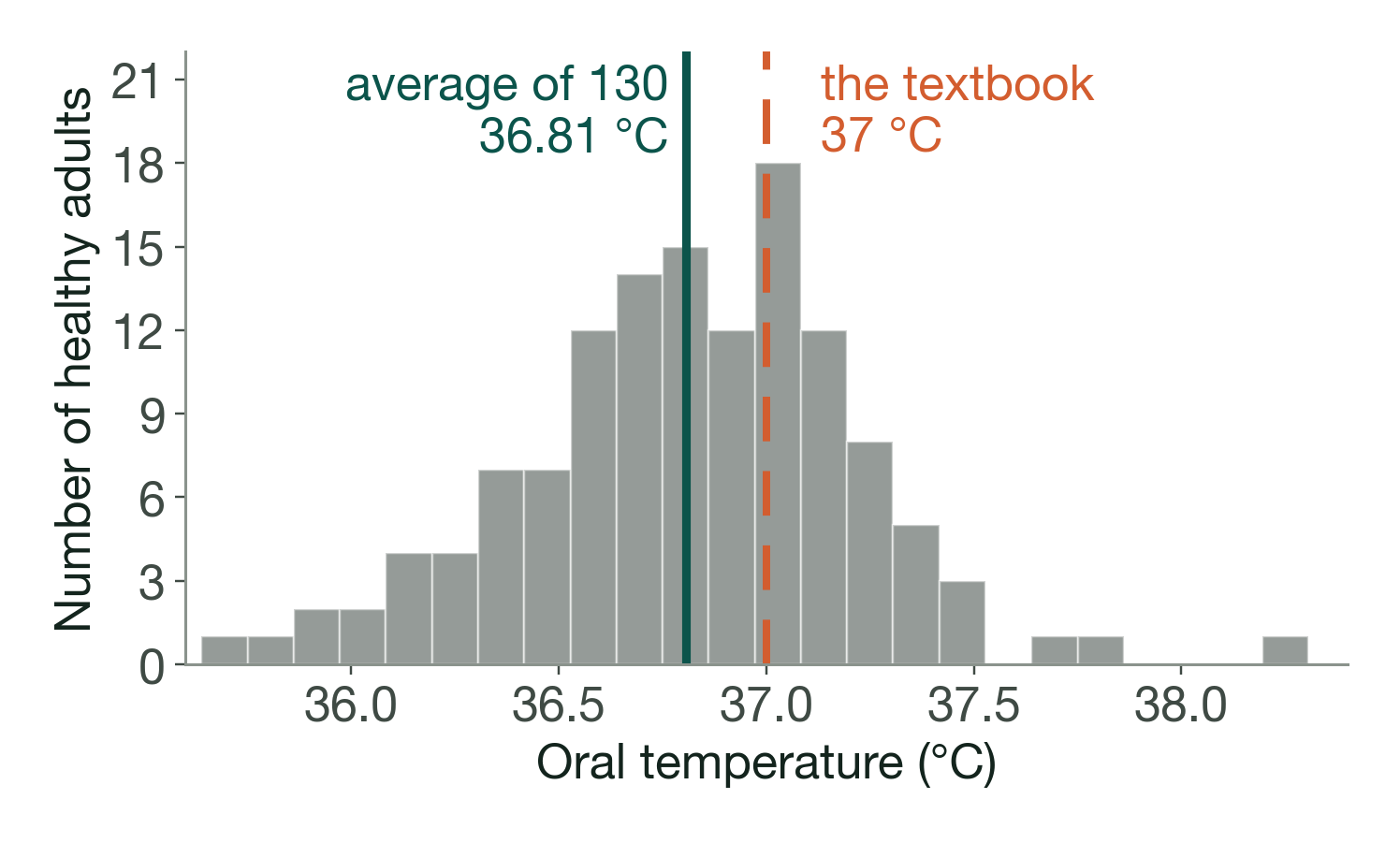
The average is a little below 37. But a different 130 people would give a different average. So the real question is: is 37 wrong, or did we draw an unlucky 130? The average alone cannot tell us. We need to know how far an average can move by chance.
Two levels: the population and the sample
| Population (the box) | Sample (the draws) | |
|---|---|---|
| What it is | all healthy adults | the 130 people measured |
| Average | \(\mu\): unknown, and fixed | \(\bar x = 36.81\): known, but it changes from sample to sample |
| SD | \(\sigma\): unknown | \(s = 0.41\) |
| Name | a parameter | a statistic; here an estimate of \(\mu\) |
2. The box model and the standard error
Picture the population as a box of tickets: one ticket for every healthy adult, with their temperature written on it. A study draws \(n\) tickets at random and takes their average. Draw again and the average changes. By how much?
The standard error of an average
The average of \(n\) random draws is centred on the box average, and typically misses it by about one standard error:
\[ \mathrm{SE} = \frac{\mathrm{SD}}{\sqrt n}, \qquad \text{here} \qquad \mathrm{SE} = \frac{0.41}{\sqrt{130}} = 0.036\ ^\circ\mathrm{C}. \]We do not know the SD of the whole box, so we use the sample's SD in its place.
The SD and the SE answer different questions. The SD (0.41 °C) says how much people differ from one another. The SE (0.036 °C) says how much the average of 130 people would change if we drew a new sample. Averages vary much less than individuals, and the more values we average, the less they vary.
In your major: replicates and the square-root law
Lab sciences In a lab you repeat a measurement and report the average of the replicates. Its SE is \(s/\sqrt n\), so precision grows only with the square root of the effort: 4 replicates halve the SE of a single reading, and halving it again takes 16. This is why "just take more measurements" runs out of steam, and why a better instrument (a smaller SD) is often the cheaper route to a precise result.
3. Why averages are predictable: the bell curve
Predict, then run
Waiting times are skewed: most are short and a few are very long. If you average 30 of them, again and again, what shape will the histogram of the averages have: skewed like the data, or bell-shaped? Predict, then open the demo with single waiting times, and step up to averages of 5 and averages of 30.
The answer is one of the most useful facts in science, the central limit theorem: for a large enough sample, the average follows the normal curve, centred on the true average, with spread equal to the SE, whatever the shape of the box. On the normal curve, 95% of the area lies within 1.96 SDs of the centre:
The engine of the confidence interval
In 95% of samples, the sample average lands within \(1.96\ \mathrm{SE}\) of the true average.
In your major: skewed measurements
BiologyEnvironmentPsychology Many science measurements are skewed: reaction times, pollutant concentrations, cell sizes, rainfall. The central limit theorem still works, but it needs larger samples. In a simulation from skewed waiting times, "average ± 1.96 SE" caught the true average in 81.0% of samples of size 5, 92.2% of size 30 and 94.3% of size 130, against the promised 95%. Before trusting an interval from a small sample, draw a histogram of the data.
4. Building a confidence interval
Turn the engine around. If the sample average is within 1.96 SE of the truth in 95% of samples, then the truth is within 1.96 SE of the sample average in those same 95% of samples: distance is the same in both directions.
A 95% confidence interval for an average
\[ \text{estimate} \pm 1.96 \times \mathrm{SE}, \qquad \text{that is,} \qquad \bar x \pm 1.96\,\frac{s}{\sqrt n}. \]The part after the ± is the margin of error.
The recipe, on the temperatures
- Estimate: the average, 36.805 °C.
- Standard error: 0.4073 / √130 = 0.0357 °C.
- Margin of error: 1.96 × 0.0357 = 0.070 °C.
- Interval: 36.805 ± 0.070, from 36.74 to 36.88 °C. Round at the end, not before.
- Answer the question: 37 °C is outside the interval. The data are not consistent with an average of 37.
In R
m  <- mean(temp)                       # 36.81
se <- sd(temp) / sqrt(length(temp))    # 0.036
m + c(-1, 1) * 1.96 * se               # 36.74 36.88
In your major: two worked examples (illustrative)
Physics Measuring g with a pendulum. A class makes 36 measurements of the acceleration due to gravity: average 9.76, SD 0.18 m s−2. SE = 0.18/√36 = 0.030; margin = 1.96 × 0.030 = 0.059; interval 9.70 to 9.82 m s−2. The accepted value, about 9.80, is inside: the class result is consistent with it.
Chemistry Vitamin C in orange juice. The label claims 40 mg per 100 mL. Titrations of 50 bottles give an average of 37.2, SD 4.1. SE = 4.1/√50 = 0.58; margin 1.14; interval 36.1 to 38.3 mg per 100 mL. The label value is outside, so chance alone does not explain the shortfall.
But: the interval covers sampling error only. If the titration systematically under-reads, or all 50 bottles came from one hot warehouse, the interval cannot know. In a lab report, discuss systematic error and how the sample was chosen next to the interval.
5. What does 95% mean?
Predict, then run
Imagine a hundred research teams. Each measures its own 130 healthy adults and builds an interval exactly as above. How many of the hundred intervals will miss the true average: none, about 5, or about 50? Commit to a number, then run the hundred teams.
In real life we can never check who was right, because we never know the true average. In a simulation we can: we choose the truth (36.8 °C), so every interval can be checked. About 95 of the hundred catch it and about 5 miss. Run it again and you may see 93 or 97; in the long run, 95%.
The meaning, four ways
Say it: "We are 95% confident that the average temperature of healthy adults is between 36.74 and 36.88 °C."
Mean it: the method catches the truth in 95% of samples. Ours is one sample, and we cannot see whether it caught.
Picture it: one ticket drawn, hand closed, from a box of 95 white and 5 black tickets. You cannot see it, but you are confident it is white.
Remember it: the truth stays put. The interval is what moves.
Check your understanding: which sentence is right?
About the interval 36.74 to 36.88 °C:
- 95% of healthy adults have a temperature between 36.74 and 36.88 °C.
- There is a 95% probability that the true average lies between 36.74 and 36.88 °C.
- If 100 teams each built an interval this way, about 95 of their intervals would contain the true average.
Vote first, convince a neighbour, then vote again.
Answer
C is right. A is about people, and people vary far more than averages: 95% of healthy adults are between about 36.81 ± 1.96 × 0.41, that is 36.0 to 37.6 °C, an interval more than ten times wider. Only 15 of the 130 people in the sample have temperatures between 36.74 and 36.88. B sounds natural, but the true average is a fixed number: it is either inside this interval or not, and the 95% belongs to the method, not to this one interval.
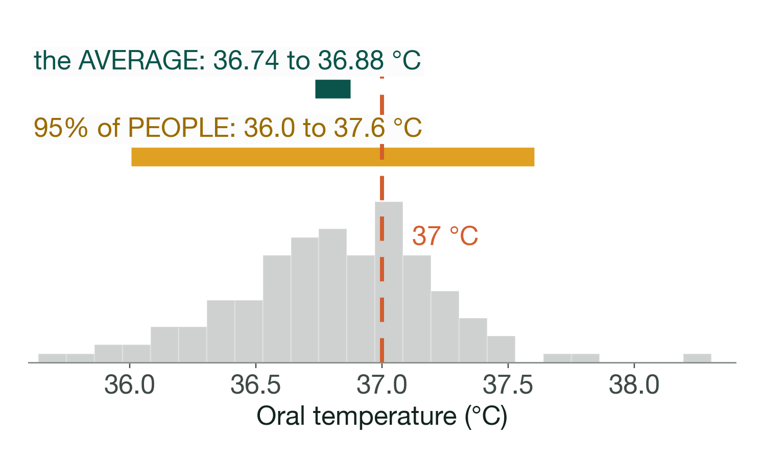
So, is 37 °C normal? For a person, yes: it sits well inside 36.0 to 37.6 °C. As the average of healthy adults, no: the interval stops at 36.88 °C.
6. Narrower intervals and planning a study
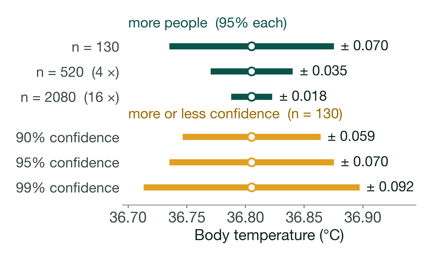
The width of the interval is \(2 \times z \times s/\sqrt n\), with multiplier \(z = 1.96\) for 95%. So three levers control it:
- More data: the width shrinks with \(\sqrt n\); four times the data halves it.
- Less spread: a smaller SD, for example a better instrument or a more uniform population.
- Less confidence: a smaller multiplier. But a narrower interval misses more often: there is no free lunch.
| Confidence level | 90% | 95% | 99% |
|---|---|---|---|
| Multiplier \(z\) | 1.645 | 1.960 | 2.576 |
| Margin of error, temperatures (\(n = 130\)) | 0.059 °C | 0.070 °C | 0.092 °C |
Planning: how many measurements?
To reach a margin of error \(E\), you need
\[ n \;\ge\; \left(\frac{z \times \mathrm{SD}}{E}\right)^{2}, \]rounded up. For the temperatures, a margin of 0.05 °C at 95% needs \((1.96 \times 0.407/0.05)^2 = 254.9\), so 255 people. Before the study the SD is unknown: use a pilot study, a published value, or a cautious guess on the high side.
In your major: better measurements beat more measurements
Physics The pendulum class (SD 0.18 m s−2) wants a margin of 0.02: \((1.96 \times 0.18/0.02)^2 = 311.2\), so 312 measurements. A smarter route is to shrink the SD: timing 20 swings and dividing by 20, instead of timing one swing, cuts the effect of reaction time on each measurement roughly twentyfold.
7. Small samples: Student's t
With 130 people, the sample SD is a very good stand-in for the true SD. With 5 people it is not: sometimes \(s\) comes out much too small, the interval is too short, and it misses. For normal data, "average ± 1.96 SE" then catches the truth only 87.8% of the time. The fix was published in 1908 by William Gosset, a chemist at the Guinness brewery in Dublin, under the pen name "Student": a larger multiplier that depends on the sample size.
| Sample size \(n\) | 5 | 10 | 30 | 130 |
|---|---|---|---|---|
| Coverage of average ± 1.96 SE (normal data) | 87.8% | 91.8% | 94.0% | 94.8% |
| Student's t multiplier for 95% | 2.776 | 2.262 | 2.045 | 1.979 |
In your major: a small sample in the lab
Earth scienceAgriculture Eight pH readings of a soil sample (illustrative): average 6.42, SD 0.21. The t multiplier for 8 readings is 2.365, so the interval is \(6.42 \pm 2.365 \times 0.21/\sqrt 8\), from 6.24 to 6.60. Using 1.96 would give 6.27 to 6.57: too short, claiming more precision than eight readings can support. With small samples, use t, and look at the data for outliers first.
In R
t.test(x)$conf.int        # the t interval for the average of the data in x
qt(0.975, df = 7) # the t multiplier for 8 readings: 2.3658. Proportions: counting yes and no
Many scientific results are counts: seeds that germinate, patients who recover, fish that carry a parasite, survey answers. Put a ticket marked 1 in the box for every "yes" and 0 for every "no". The average of the tickets is then the proportion of yes, and everything above still works:
\[ \hat p = \frac{\text{number of yes}}{n}, \qquad \mathrm{SE} = \sqrt{\frac{\hat p\,(1-\hat p)}{n}}, \qquad \text{interval: } \hat p \pm 1.96 \times \mathrm{SE}. \]Example: seed germination (illustrative)
A seed company claims that 80% of its seeds germinate. In a trial, 108 of 150 seeds germinate: \(\hat p = 0.72\), SE = \(\sqrt{0.72 \times 0.28/150} \)
This interval relies on the bell curve, so it needs enough of both outcomes: as a rule of thumb, at least about 5 yes and 5 no. With fewer, use the exact binomial methods (in R, binom.test). Going further: why is \(\hat p\) the natural estimate? The likelihood demonstration shows it is the value that makes the observed data most probable.
In R
prop.test(108, 150, correct = FALSE)$conf.int    # 0.643 0.786 (a close cousin of the hand calculation)
binom.test(108, 150)$conf.int # 0.641 0.790 (exact)9. Testing a claim: P-values
A confidence interval says which values are consistent with the data. A hypothesis test asks about one value: could the true average be exactly 37 °C?
The logic of a test, in four steps
- The claim to test, the null hypothesis \(H_0\): the true average is 37 °C. The alternative \(H_1\): it is not.
- Assume \(H_0\) is true and measure how far the data are from it, in standard errors: \(t \)
\({}= (\bar x - 37)/\mathrm{SE} \) \({}= (36.81 - 37)/0.036 \) \({}= -5.28\). - The P-value: if \(H_0\) were true, how often would chance alone put a sample average at least this far from 37? Here about 5 times in 10 million samples: \(P \approx 5 \times 10^{-7}\).
- Decide: a small P-value (by convention, below 0.05) means the data would be very surprising if \(H_0\) were true, so we reject \(H_0\): the average is not 37 °C.
These numbers use the rounded summaries; the full data give \(t = -5.46\) and \(P \approx 2\times10^{-7}\). The conclusion is the same.
What a P-value is not
- Not the probability that \(H_0\) is true. It is computed assuming \(H_0\) is true: it measures how surprising the data would be.
- Not the size of the effect. A tiny difference can give a tiny P-value in a large study. Here the difference from 37 is only 0.19 °C: real, but small. The interval shows the size; the P-value does not.
- A large P-value does not prove \(H_0\). "No evidence of a difference" is not "evidence of no difference": the study may simply be too small.
Tests and intervals agree. A two-sided test at the 5% level rejects a value exactly when that value lies outside the 95% confidence interval. 37 is outside 36.74 to 36.88, so the test rejects it. Papers report both; the interval tells you more.
Two ways to be wrong, and how many samples you need
A test can reject a true claim (a false alarm, or Type I error, which happens 5% of the time when the claim is true and we test at the 5% level) or miss a real effect (a missed effect, or Type II error). The chance of detecting a real effect is the power. Power grows with the size of the effect and with the sample size, so planning a study means choosing a sample size that gives enough power.
In your major: how many plants, mice or patients per group?
BiologyHealthPsychology To compare two groups with 80% power at the 5% level, you need about 64 per group to detect a difference of half an SD, and about 26 per group for a difference of 0.8 SD. Small effects are expensive: halving the effect you want to detect needs about four times the sample. Animal ethics committees and funding bodies ask for this calculation before an experiment starts.
In R
power.t.test(delta = 0.5, sd = 1, power = 0.8)    # n = 63.8, so 64 per group
power.t.test(delta = 0.8, sd = 1, power = 0.8) # n = 25.5, so 26 per group10. Comparing two groups
Most experiments compare: treatment against control, one site against another, before against after. The questions are the same as before: is the difference real, or could chance alone have produced it? And how big is it?
Two independent groups
Example: does a treatment increase plant growth? (real data)
In a classic experiment, the dried weights of 10 plants grown under a control condition were compared with those of 10 plants grown under a treatment (Dobson, 1983; the data are built into R as PlantGrowth). Control: average 5.03 g (SD 0.58). Treatment: average 5.53 g (SD 0.44).
The difference is 0.49 g, with 95% confidence interval 0.005 to 0.98 g and P = 0.048 (Welch's two-sample t-test, which does not assume that the two groups have the same spread). The interval only just excludes 0: the treatment probably helps, but the gain could be tiny or close to 1 g. With 10 plants per group, that is all the precision the experiment can give.
A second treatment in the same experiment gave P = 0.25. Not significant, but its interval for the change, −1.03 to 0.29 g, allows a sizeable loss or a small gain: not significant does not mean no effect.
Overlapping intervals are not a test. Split the temperatures by sex: men 36.72 °C (95% CI 36.63 to 36.82), women 36.89 °C (95% CI 36.79 to 36.99). The two intervals overlap, yet the interval for the difference, 0.16 °C, runs from 0.02 to 0.30 and excludes 0. To compare two groups, build an interval for the difference, not two intervals side by side.
Paired designs: the same subjects twice
Example: two sleeping drugs on the same patients (real data, 1905)
Ten patients each tried two sleeping drugs, and the extra hours of sleep were recorded (Cushny and Peebles, 1905; analysed by "Student" in 1908; built into R as sleep). Drug 1: average 0.75 h extra. Drug 2: average 2.33 h extra.
Each patient's difference (drug 2 minus drug 1) averages 1.58 h, with 95% CI 0.70 to 2.46 h and P = 0.003 (paired t-test). Ignoring the pairing, as if 20 different people had been measured, gives a much wider interval, −0.21 to 3.37 h, and P = 0.08. The reason: patients differ a lot from one another (a patient's two results are strongly related, correlation 0.80), and the paired analysis removes that person-to-person variation.
In your major: designing a paired experiment
BiologyChemistryHealth Pair whenever you can: the same patient before and after treatment, two halves of the same leaf, the same water sample measured by two methods, neighbouring field plots with one treated and one not. Then analyse the differences. Pairing must be planned: data collected as two separate groups cannot be paired afterwards.
In R
pg <- droplevels(subset(PlantGrowth, group != "trt1"))
t.test(weight ~ group, data = pg)                     # Welch: control minus treatment
with(sleep, t.test(extra[group == 2], extra[group == 1], paired = TRUE)) # paired11. Reporting and reading results
In a lab report
"The average oral temperature was 36.81 °C (95% CI 36.74 to 36.88 °C; \(n = 130\))." Give the estimate, the interval with its level, the units and the sample size, and round to the precision of the measurements. For a test, add the statistic and the P-value: "The average differed from 37 °C (\(t = -5.46\), 129 degrees of freedom, \(P < 0.001\))."
Reading a paper. You will meet sentences like "mean difference 2.3 (95% CI 0.4 to 4.2)". Read it as: the study's best estimate is 2.3, and values from 0.4 to 4.2 are consistent with the data. An interval that excludes 0 corresponds to a result that is "statistically significant at the 5% level", and it also shows how large or small the effect could plausibly be, which the bare word "significant" does not.
Common mistakes: check your sentence against these
- About people, not the average. The interval is for the population average; most individuals lie far outside it.
- Probability on the fixed average. Say "95% confident", and remember that the 95% describes the method.
- Forgetting what it does not cover. Measurement bias, a non-random sample (volunteers, one site, one season) or observations that are not independent are not in the margin of error.
- Treating overlap as a test. Two overlapping intervals can still come from a clear difference.
- "95% of future averages will fall in this interval." Not so: a repeat study's average lands inside the original 95% interval only about 83% of the time.
- Reading P as the probability that the claim is true, or a non-significant result as proof of no effect.
- Missing units, sample size or level, or rounding before the end of the calculation.
12. Exercises
Try each one first, then open the answer.
Seagrass (illustrative). A marine biologist measures 49 seagrass shoots in one bay: average length 21.5 cm, SD 7 cm. (a) Give a 95% confidence interval for the average shoot length in the bay. (b) Explain it to a park ranger in one sentence. (c) How many shoots would halve the width?
Answer
(a) SE = 7/√49 = 1 cm, so 21.5 ± 1.96: from 19.5 to 23.5 cm. (b) "We are 95% confident that the average length of the seagrass shoots in this bay is between 19.5 and 23.5 cm." (c) 4 × 49 = 196 shoots.
Coffee (illustrative). 100 cups of coffee from one café contain on average 95.2 mg of caffeine, SD 12.5 mg. Is an average of 100 mg per cup consistent with these data?
Answer
SE = 12.5/√100 = 1.25 mg; interval 95.2 ± 2.45, from 92.8 to 97.6 mg. 100 mg is outside, so it is not consistent with these data.
True or false? For the temperature interval 36.74 to 36.88 °C: (a) about 95% of the 130 people in the sample have temperatures in this range; (b) with 520 people instead of 130, the interval would be about half as wide; (c) a 99% interval from the same data would be narrower; (d) the interval would still answer the question if all 130 people had been measured an hour after exercise.
Answer
(a) False: the interval is for the average; only 15 of the 130 people (12%) have temperatures in it. (b) True: 520 = 4 × 130. (c) False: it would be wider, with multiplier 2.576. (d) False: it would describe the average temperature after exercise, a different population; a systematic shift is not in the margin of error.
Reaction times (illustrative). 120 students have an average simple reaction time of 318 ms, SD 74 ms. (a) Give a 95% interval for the average. (b) A student says "so my reaction time is almost certainly between 305 and 331 ms". Correct them.
Answer
(a) SE = 74/√120 = 6.76 ms; interval 318 ± 13.2, from 305 to 331 ms. (b) That range is for the average of students. Individuals vary with SD 74 ms, so a rough 95% range for one student is 318 ± 1.96 × 74, about 173 to 463 ms (rough, because reaction times are skewed).
Planning a water survey. A pilot study of nitrate in a creek gives an SD of 2.4 mg/L. How many water samples give a 95% margin of error of 0.5 mg/L?
Answer
(1.96 × 2.4/0.5)² = 88.5, rounded up: 89 samples.
An exam-style question: Sydney rock oysters (illustrative). A farm measures 64 oysters: average shell length 62 mm, SD 8 mm. (a) Give a 95% interval for the average shell length of the farm's oysters. (b) Explain it to the farmer in one sentence. (c) How many oysters would halve the width of the interval?
Answer and marking
(a) SE = 8/√64 = 1 mm, so 62 ± 1.96: from 60.0 to 64.0 mm. (b) "We are 95% confident that the average shell length of this farm's oysters is between 60 and 64 mm." (c) 4 × 64 = 256 oysters.
How a sentence like (b) is marked, one point each: it is about the average, not single oysters; it names the population and the units (this farm's oysters, mm); and its 95% describes the method ("confident", not "a 95% probability").
Reading a P-value. The plant experiment of Section 10 gave P = 0.048. Which reading is right? (a) There is a 4.8% chance that the treatment has no effect. (b) If the treatment had no effect, a difference at least this large would turn up in about 4.8% of experiments like this one. (c) The treatment increases dried weight by 4.8%.
Answer
(b). The P-value is computed assuming no effect, so it cannot be the probability of no effect (a); and it says nothing about the size of the effect (c): the interval, 0.005 to 0.98 g, does that.
Paired or independent? Choose the analysis for each study. (a) Blood pressure of 30 patients before and after a drug. (b) Heights of 30 plants in sunny plots and of 30 other plants in shaded plots. (c) Lead concentration in 20 water samples, each measured by two laboratories.
Answer
(a) Paired: the same patients twice. (b) Independent groups: Welch's two-sample t-test. (c) Paired: each water sample is measured twice, so analyse the 20 differences between the laboratories.
A new batch of seeds (illustrative). In a second trial, 164 of 200 seeds germinate. Is the company's claim of 80% consistent with this batch?
Answer
\(\hat p = 0.82\), SE = \(\sqrt{0.82 \times 0.18/200} \)
\({}= 0.027\), interval 0.82 ± 0.053, from 76.7% to 87.3%. The claimed 80% is inside, so this batch is consistent with the claim (unlike the batch in Section 8).
Demonstrations
Ten interactive experiments that run in your browser, with no installation. Each opens with ready-made scenarios under Try these; make a prediction before you run one.
| Demonstration | Try this | Sections |
|---|---|---|
| Averages on trial | Skewed waiting times averaged over 1, 5 and 30 values: watch the bell curve appear | 2, 3 |
| Confidence intervals: does the method catch the truth? | A hundred teams at once; then only five people each, with 1.96 and with t | 5, 6, 7 |
| Why Student's t? | Why small samples need the larger t multiplier, and when normality matters | 7 |
| Counting successes | How well the interval for a proportion really covers the truth | 8 |
| Tests and intervals | Drag a claimed value across the interval and watch the P-value | 9 |
| A hypothesis test on trial | Thousands of tests: false alarms at 5%, and power | 9 |
| Power and sample size | How many people for 80% power? | 9 |
| Two samples | Paired against unpaired; pooled against Welch | 10 |
| Estimators on trial | Going further: why the SD divides by \(n-1\) | 2 |
| Maximum likelihood | Going further: where estimates such as \(\hat p\) come from | 8 |
References
- Freedman, D., Pisani, R. and Purves, R. (2007). Statistics, 4th edition. W. W. Norton, New York. The box model of these notes comes from this book.
- Diez, D. M., Çetinkaya-Rundel, M. and Barr, C. D. (2019). OpenIntro Statistics, 4th edition. OpenIntro. A free textbook: openintro.org/book/os.
- Shoemaker, A. L. (1996). What's normal? Temperature, gender, and heart rate. Journal of Statistics Education, 4(2). doi:10.1080/10691898.1996.11910512.
- Mackowiak, P. A., Wasserman, S. S. and Levine, M. M. (1992). A critical appraisal of 98.6 °F, the upper limit of the normal body temperature, and other legacies of Carl Reinhold August Wunderlich. JAMA, 268(12), 1578–1580. doi:10.1001/jama.1992.03490120092034.
- Dobson, A. J. (1983). An Introduction to Statistical Modelling. Chapman and Hall, London. Source of the plant-growth data.
- Cushny, A. R. and Peebles, A. R. (1905). The action of optical isomers. II. Hyoscines. The Journal of Physiology, 32(5–6), 501–510. doi:10.1113/jphysiol.1905.sp001097.
- Student (1908). The probable error of a mean. Biometrika, 6(1), 1–25. doi:10.1093/biomet/6.1.1.
- Hoekstra, R., Morey, R. D., Rouder, J. N. and Wagenmakers, E.-J. (2014). Robust misinterpretation of confidence intervals. Psychonomic Bulletin & Review, 21(5), 1157–1164. doi:10.3758/s13423-013-0572-3. Even researchers misread confidence intervals.
- Cumming, G. (2014). The new statistics: why and how. Psychological Science, 25(1), 7–29. doi:10.1177/0956797613504966. Why to report intervals, not only P-values.
The pendulum, vitamin C, soil pH, germination, seagrass, coffee, reaction-time, nitrate and oyster examples are illustrative numbers constructed for these notes. The temperature, plant-growth and sleep data are real. All numbers were computed in R.